Embed Size (px)
Citation preview

Adjustment Costs, Firm Responses, and Labor Supply Elasticities: Evidence from Danish Tax Records
Raj Chetty, Harvard University and NBER
John N. Friedman, Harvard University and NBER
Tore Olsen, Harvard University and CAM
Luigi Pistaferri, Stanford University and NBER
March 2010
Introduction
• How do taxes affect labor supply and earnings behavior?
• Most find intensive margin elasticities near zero (Heckman 1993, Blundell and MaCurdy 1999, Saez et al 2009)
• Literature assumes that workers may freely choose labor supply
• Two factors prevent workers from choosing labor supply freely:
• Search costs in finding optimal job
• Constraints imposed by firms (e.g. hours constraints)
• Because of these frictions, workers may not reoptimize in response to tax changes of small size and scope in short run
Micro elasticity estimates may be attenuated relative to elasticities relevant for macro comparisons

Overview
• Derive three testable predictions about how adjustment costs and hours constraints affect micro labor supply elasticity estimates
• Test predictions using an administrative tax panel for the population of Denmark
• Find that standard micro methods of estimating elasticities on this dataset yields elasticities close to zero
• But accounting for frictions produces sharp evidence of larger elasticities and explains why standard approach is biased
• Calibration suggests that micro elasticity estimates understate the macro elasticities by an order of magnitude

Model with Search Costs and Endogenous Institutional Constraints
• Two types of labor supply models in existing literature
• Neo-classical: workers freely choose hours
• Hours constraints: wage-hours packages determined by firms’ production technologies (Rosen 1976, Blundell et al. 2008)
• This paper: model of endogenous hours constraints
• Wage-hours packages offered by firms reflect workers’ aggregate preferences
• But workers face search frictions, so each worker is not at his individual optimum

Model Setup
• Workers: Constant elasticity quasi-linear utility function
• c is consumption and i is an individual taste parameter
• Smooth distribution F(i ) in the economy
• Firms: CRS Leontief production function
• Offers (possibly heterogeneous) wage-hours packages {hj , wj }
• Workers all produce goods sold a price p
• Firm size Nj determined endogenously in equilibrium
uic,h c − i−1/ h 11/
11/
j pNj minhj1 , . . . ,hj
Nj − wj∑i1
Nj
hji

Model Setup
• Search Frictions:
• Workers initially draw job with wage-hours package {h0 ,w0 } from distribution G(.) offered by firms
• Two ways to switch jobs:
1. Switch to job with same hours but higher wage at no cost (e.g., no re-training required)
2. Switch to different hours by paying a cost:
• Draw new wage-hours package {h’,w’} from Ge (.|hi *)
• Draw centered at optimal job, E(h’ | hi *) = hi *
• Variance decreasing in effort, Var(h’) = k(1 – e)
• Search cost e weakly increasing in effort e

Model Setup
• Equilibrium:
• Firm maximize profits
• All workers paid same wage wj = w = p
• Workers choose optimal search effort (or not to search at all)
• Workers only search if utility gain ui (h*) - ui (h0 ) > (ei *)
• Market clears: Supply equals demand at each hours level
• Search process does not change the hours distribution
h0 ∉ h i, h i
Gh FGhF.

Estimating Elasticities: Benchmark Frictionless Model
• Special case: (e) = 0, all workers choose hi = hi *
• Structural parameter
determines wage elasticity of labor supply
• Two micro methods of identifying structural elasticity
1. Variation in tax rates over time. For individuals affected by tax change, observed hours elasticity w.r.t. net-of-tax wage equals
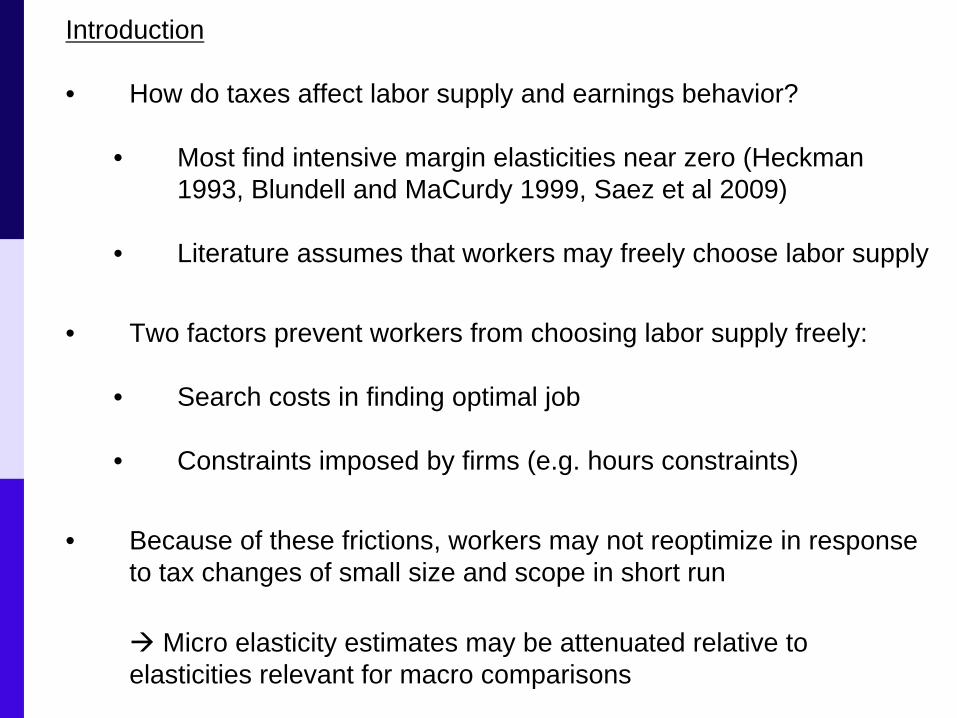
2. Variation in rates across tax brackets. Amount of bunching at kinks can be used to estimate
d loghd log1−
Bunching at Kink Points
Income distribution
Income/Labor Supply
Consumption Before Kink Introduction After Kink Introduction
Budget Set

Bunching at Kink Points
Income distribution
Income/Labor Supply
Budget Set

Bunching at Kink Points
Income distribution
Income/Labor Supply
Consumption Before Kink Introduction After Kink Introduction
Budget Set

Bunching at Kink Points
Income distribution after kink introduction
Consumption Before Kink Introduction After Kink Introduction
Income/Labor Supply
“By the end of November some of my colleagues stop working. It does not pay anymore because they have reached the high tax bracket.”
- Danish construction worker

Consumption Before Kink Introduction After Kink Introduction
Income/Labor Supply
Bunching at Kink Points
B2−1
Saez
(2002):

Baseline Case: Estimating Elasticities
• Special case: (e) = 0, all workers choose hi = hi *
• Structural parameter
determines wage elasticity of labor supply
• Two micro methods of identifying structural elasticity
1. Variation in tax rates over time. For individuals affected by tax change, observed hours elasticity w.r.t. net-of-tax wage equals
2. In non-linear tax system, use variation in rates across tax brackets. Examine amount of bunching at the kink.
How do frictions affect estimated elasticities?
d loghd log1−

Bunching with Search Frictions
• With hour constraints, there are two ways to locate at the kink
1. Individual Bunching: Workers search for a job at the kink
2. Firm Bunching: Draw job at kink to begin with
• Signature of firm bunching: Even workers who do not face a kink bunch there
• Three predictions about observed elasticity measured from bunching at kink
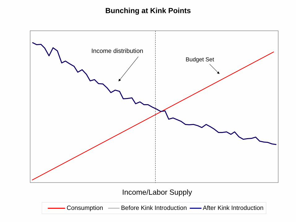
Effects of Frictions on Observed Elasticities
• Three empirical predictions:
1. [Size] Larger kinks generate larger observed elasticities
• Large kinks are more likely to induce workers to pay search costs and relocate to the kink

Labor Supply
Con
sum
ptio
n
h*h h_
_
U(c,h) = U*
U(c,h) = U* – φ
Slope = (1 – 2 )w
Slope =(1 – 1 )w

Labor Supply
Con
sum
ptio
n
h*h h_
_
U(c,h) = U*
U(c,h) = U* – φ
_h’
Slope = (1 – 2 )w
Slope =
Slope = (1 –
’)w
(1 – 1 )w

Effects of Frictions on Observed Elasticities
• Three empirical predictions:
1. [Size] Larger kinks generate larger observed elasticities
• Large kinks are more likely to induce workers to pay search costs and relocate to the kink
2. [Scope] Kinks that affect a larger group of workers generate larger observed elasticities
• Firms tailor jobs to aggregate preferences more firm bunching at common kinks
3. [Correlation] More firm bunching in sectors with greater individual bunching
• In sectors of the economy where workers are more elastic, firms offer more jobs at the kink.

Micro vs Macro Elasticities
• Define macro elasticity as effect of difference in tax rates across economies on average hours of work:
• In frictionless model, observed elasticities coincide with structural elasticity irrespective of size and scope
No difference between micro and macro elasticities
• In our model, macro elasticity coincides with
even with frictions
• But micro estimates are attenuated
• Intuition: micro estimates identified from “fine tuning” of hours in response to tax changes or locating at kinks
MAC E logh i1′ −E logh i1
log1−1′ −log1−1

DATA AND INSTITUTIONAL BACKGROUND
• Matched employer-employee panel data with admin tax records for full population
• Income vars: wage earnings, capital and stock income, pension contributions
• Employer vars: tenure, occupation, employer ID
• Demographics: education, spouse ID, kids, municipality
• Sample restriction: Wage-earners aged 15-70, 1994-2001
• Approximately 2.42 million people per year

Marginal Tax Rates in Denmark in 200060
020
4080
100 200 300 40050 150150 250 350Taxable Income (1000s DKR)
Mar
gina
l Tax
Rat
e (%
)
log(NTR) = -11%
log(NTR) = -33%
Note: $1
6 DKr

KEY FEATURES OF TAX SYSTEM 1994-2001
• Taxable income = wage earnings + net deductions
• Wage earnings: double reported by firms and workers
• Net deductions:
• Non-wage income: gifts, awards, company cars
• Deductions: pension contributions, some work expenses
• Question of shifting vs. "real" labor supply responses
• Top bracket cutoffs move over time
• Indexed to two-year lagged earnings growth: tax policy set before earnings choices are made

Movement in Top Tax Cutoff Across Years
Year
2000
DK
R (1
000s
)
Nom
inal
DK
R (1
000s
)
262
264
266
268
270
272
1994 1995 1996 1997 1998 1999 2000 2001230
240
250
260
270
280
CPI Adjusted Nominal

Income Distribution for Wage Earners Around Top Kink (1994-2001)20
000
4000
060
000
8000
010
0000
-50 -40 -30 -20 -10 0 10 20 30 40 50
Taxable Income Relative to Top Bracket Cutoff (1000s DKr)
Freq
uenc
y

Income Distribution for Wage Earners Around Top Kink (1994-2001)20
000
4000
060
000
8000
010
0000
-50 -40 -30 -20 -10 0 10 20 30 40 50
Taxable Income Relative to Top Bracket Cutoff (1000s DKr)
Freq
uenc
y
Excess mass BΔ

Income Distribution for Wage Earners Around Top Kink (1994-2001)20
000
4000
060
000
8000
010
0000
-50 -40 -30 -20 -10 0 10 20 30 40 50
Taxable Income Relative to Top Bracket Cutoff (1000s DKr)
Freq
uenc
y
Excess mass (b) = 0.81 Standard error = 0.05
1000
020
000
3000
0
1000
020
000
3000
0
-50 -40 -30 -20 -10 0 10 20 30 40 50
0Fr
eque
ncy
(mar
ried
wom
en)
Freq
uenc
y (s
ingl
e m
en)
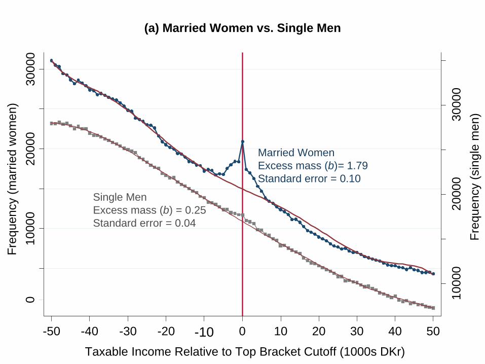
(a) Married Women vs. Single Men
Taxable Income Relative to Top Bracket Cutoff (1000s DKr)
Married WomenExcess mass (b)= 1.79Standard error = 0.10
Single MenExcess mass (b) = 0.25Standard error = 0.04

010
0020
0030
0040
00
020
0040
0060
0080
00
-50 -40 -30 -20 -10 0 10 20 30 40 50
(b) Teachers vs. MilitaryFr
eque
ncy
(teac
hers
)
Freq
uenc
y (m
ilita
ry)
Taxable Income Relative to Top Bracket Cutoff (1000s DKr)
TeachersExcess mass (b)= 3.54Standard error = 0.25
MilitaryExcess mass (b) = -0.12Standard error = 0.21

Freq
uenc
y (a
ll w
age
earn
ers)
Freq
uenc
y (m
arrie
d w
omen
)0
1000
2000
3000
4000
6000
8000
1000
012
000
1400
0
210 220 230 240 250 260 270 280 290 300Taxable Income (1000s DKR)
All Wage Earners
Married Women
Taxable Income Distributions in 1994

1000
2000
3000
0
4000
8000
1200
01995
210 220 230 240 250 260 270 280 290 300Taxable Income (1000s DKR)
Freq
uenc
y (a
ll w
age
earn
ers)
Freq
uenc
y (m
arrie
d w
omen
)

1000
2000
3000
0
4000
8000
1200
01996
210 220 230 240 250 260 270 280 290 300Taxable Income (1000s DKR)
Freq
uenc
y (a
ll w
age
earn
ers)
Freq
uenc
y (m
arrie
d w
omen
)

010
0020
0030
00
5000
1000
015
000
1997
210 220 230 240 250 260 270 280 290 300Taxable Income (1000s DKR)
Freq
uenc
y (a
ll w
age
earn
ers)
Freq
uenc
y (m
arrie
d w
omen
)

010
0020
0030
00
4000
8000
1200
01998
210 220 230 240 250 260 270 280 290 300Taxable Income (1000s DKR)
Freq
uenc
y (a
ll w
age
earn
ers)
Freq
uenc
y (m
arrie
d w
omen
)

010
0020
0030
0040
00
4000
8000
1200
01999
210 220 230 240 250 260 270 280 290 300Taxable Income (1000s DKR)
Freq
uenc
y (a
ll w
age
earn
ers)
Freq
uenc
y (m
arrie
d w
omen
)

1000
2000
3000
4000
0
6000
1000
014
000
2000
210 220 230 240 250 260 270 280 290 300Taxable Income (1000s DKR)
Freq
uenc
y (a
ll w
age
earn
ers)
Freq
uenc
y (m
arrie
d w
omen
)

1000
2000
3000
4000
6000
1000
014
000
2001
210 220 230 240 250 260 270 280 290 300Taxable Income (1000s DKR)
Freq
uenc
y (a
ll w
age
earn
ers)
Freq
uenc
y (m
arrie
d w
omen
)

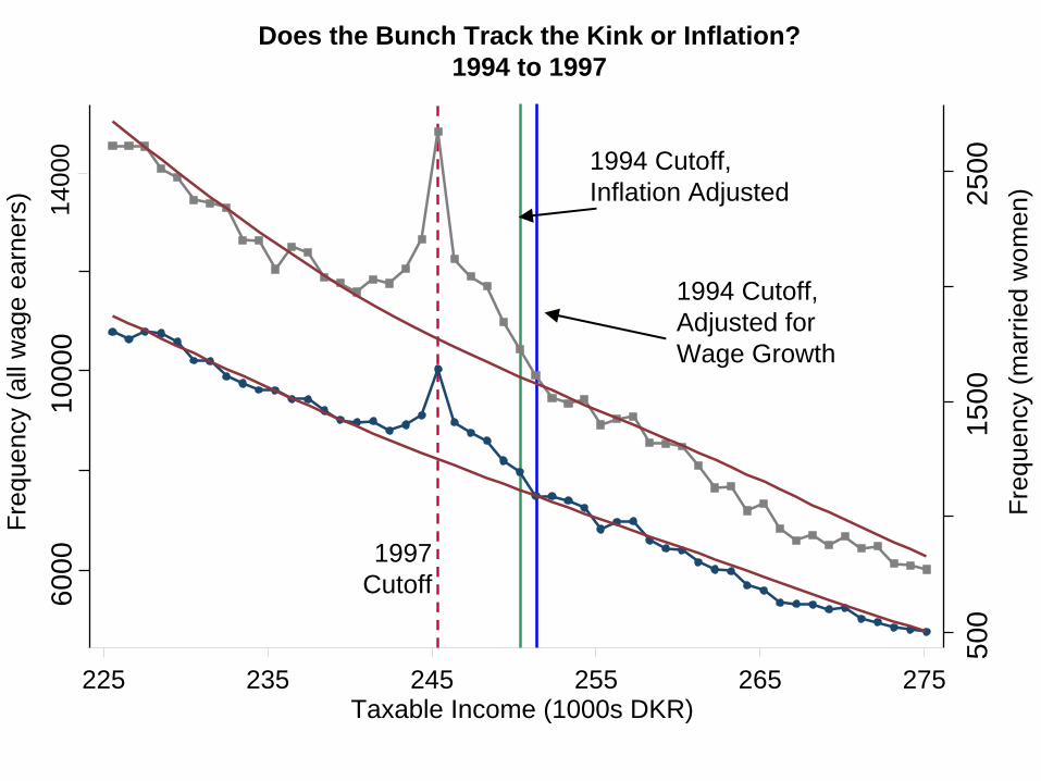
Does the Bunch Track the Kink or Inflation? 1994 to 1997
6000
1000
014
000
225 235 245 255 265 275Taxable Income (1000s DKR)
500
1500
2500
Freq
uenc
y (m
arrie
d w
omen
)
Freq
uenc
y (a
ll w
age
earn
ers)

1997 Cutoff
1994 Cutoff, Inflation Adjusted
1994 Cutoff, Adjusted for Wage Growth
Does the Bunch Track the Kink or Inflation? 1994 to 1997
6000
1000
014
000
225 235 245 255 265 275Taxable Income (1000s DKR)
500
1500
2500
Freq
uenc
y (m
arrie
d w
omen
)
Freq
uenc
y (a
ll w
age
earn
ers)
500
1500
2500
6000
1000
014
000 1994 Cutoff,
Inflation Adjusted
1994 Cutoff, Adjusted for Wage Growth
225 235 245 255 265 275
Freq
uenc
y (a
ll w
age
earn
ers)
Freq
uenc
y (m
arrie
d w
omen
)
Taxable Income (1000s DKR)
Does the Bunch Track the Kink or Inflation? 1994 to 1997
1997 Cutoff

1000
2000
3000
6000
1000
014
000
255 265 275 285 295 305
Freq
uenc
y (a
ll w
age
earn
ers)
Taxable Income (1000s DKR)
Freq
uenc
y (m
arrie
d w
omen
)
1997 Cutoff, Inflation Adjusted
Actual 2001 Cutoff
1997 Cutoff, Adjusted for Wage Growth
Does the Bunch Track the Kink or Inflation? 1997 to 2001

LABOR SUPPLY RESPONSES VS. SHIFTING
• Does bunching reflect earnings responses or income shifting?
• Two mechanisms for income shifting
1. Evasion: under-reporting of income to avoid higher tax
• Kleven et al. (2009) audit study: no evasion in wage earnings
• Could still have mis-reporting of non-wage income
Test: Bunching in wage earnings?
2. Shift to nontaxable compensation (pension contributions)
Test: Bunching in pensions plus taxable income?

Distribution of Wage Earnings20
000
4000
060
000
8000
0
-50 -40 -30 -20 -10 0 10 20 30 40 50
Freq
uenc
y
Income Measure Relative to Top Bracket Cutoff (1000s DKR)
Excess mass (b) = 0.68Standard error = 0.05

Distribution of Taxable Income Plus Pensions20
000
4000
060
000
8000
0
-50 -40 -30 -20 -10 0 10 20 30 40 50
Freq
uenc
y
Income Measure Relative to Top Bracket Cutoff (1000s DKR)
Excess mass (b)= 0.48Standard error = 0.04

PREDICTION 1: Small vs. Large Tax Changes
• We have already examined the larger, top tax kink
• Top Bracket Cutoff: log(NTR)
30%
• Two sources of smaller tax variation:
• Middle Bracket Cutoffs: log(NTR)
10%
• Small Tax Reforms
• Now estimate observed elasticities from bunching at smaller kinks and small tax reforms

4000
060
000
8000
010
0000
1200
00
-50 -40 -30 -20 -10 0 10 20 30 40 50
Middle Tax Kink: All Wage Earners, Taxable Income Distribution
Excess mass (b) = 0.06Standard error = 0.03
Predicted excess mass = 0.16Standard error = 0.01
Taxable Income Relative to Middle Bracket Cutoff
Freq
uenc
y

5000
060
000
7000
080
000
9000
010
0000
-50 -40 -30 -20 -10 0 10 20 30 40 50
Middle Tax Kink: All Wage Earners, Wage Earnings Distribution
Wage Earnings Relative to Middle Bracket Cutoff
Freq
uenc
y
Excess mass (b) = -0.06Standard error = 0.03
Predicted excess mass = 0.14 Standard error = 0.01

1000
020
000
3000
040
000
-50 -40 -30 -20 -10 0 10 20 30 40 50
Middle Tax Kink: Married Women, Taxable Income Distribution
Taxable Income Relative to Middle Bracket Cutoff
Freq
uenc
y
Excess mass (b) = 0.06Standard error = 0.03
Predicted excess mass = 0.35Standard error = 0.02

PREDICTION 1: Small vs. Large Tax Changes
• Tax Reforms
• Many small reforms during period we study: 4% change in net-of-tax wage on average
• Methodology: Gruber and Saez (2002)
• Regress 2-year income change on 2-year change in net-of-tax wage (1-MTR)
• Instrument for actual change in (1-MTR) with simulated change holding fixed base year characteristics
• Include 10-piece spline in income and various fixed effects

Year Fixed Effects
Observed Elasticity Estimates Using Small Tax Reforms
Variable:All Wage Earners
MarriedFemales
Married Fem.Professionalsw/ High Exp.
WageEarners> 200K
(1) (2) (3) (4) (5)Subgroup:
% Change in NTR -0.005 -0.007 0.002 0.001 -0.001
Labor Income Spline
Sample Size
(0.003) (0.004) (0.005) (0.011) (0.003)
11,512,625 8,189,920 3,136,894 156,527 7,480,900
x x x x x
Total Income Spline x x x x
x x x x x
Age Fixed Effects x x x x x
Occupation Fixed Effs. x
Region Fixed Effects x
Dependent Variable: % Change in Labor Income:
Gender/Married FE x
x
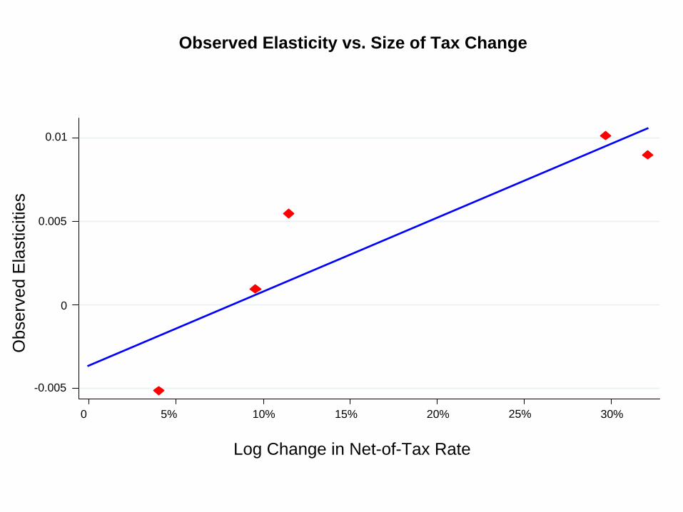
Observed Elasticity vs. Size of Tax Change
Log Change in Net-of-Tax Rate
Obs
erve
d E
last
iciti
es
0 10% 20% 30%5% 15% 25%
0
0.005
0.01
-0.005

Switchers from Top Tax to Middle TaxFr
eque
ncy
(Mid
dle
Tax)
Taxable Income Relative to Bracket Cutoff
Freq
uenc
y (T
op T
ax)
050
0010
000
1500
020
000
5000
1000
015
000
2000
0
-25 -15 -5 5 15 25
Excess mass (b) = 0.54Standard error = 0.08
Excess mass (b) = 0.06Standard error = 0.07
Middle Tax, year t+2Top Tax, year t

PREDICTION 2: Firm Responses and Scope of Kinks
• Do tax incentives that affect a larger group of workers generate larger elasticities?
• Need variation in size of group affected by a tax change
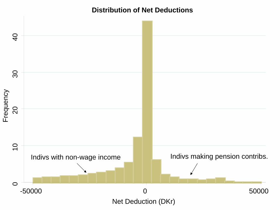
• Exploit variation in deductions and non-wage income across workers
• Creates variation in effective location of top bracket cutoff (the labor income required to be just at the top bracket)
• We focus on two kinks:
• Statutory top tax kink, faced by 60% of population
• “Pension” kink, faced by 2.5% of population
010
2030
40
-50000 0 50000
Distribution of Net Deductions
Net Deduction (DKr)
Freq
uenc
y
Indivs making pension contribs.Indivs with non-wage income

05
1015
20
20000 30000 40000 50000
Distribution of Net Deductions Given Deductions > DKr 20,000
Net Deduction (DKr)
Freq
uenc
y

PREDICTION 2: Firm Responses and Small vs. Large Groups
• Prediction 2.1: There is firm bunching at the statutory top tax cutoff
• Firms should have excess propensity to structure jobs so that salaries are close to statutory top bracket cutoff because 60% of workers face that cutoff
• Signature of firm bunching: bunching among people who do not face a given change in tax incentives
• Examine wage earnings distribution at occupation level because of prevalence of collective wage bargaining in Denmark
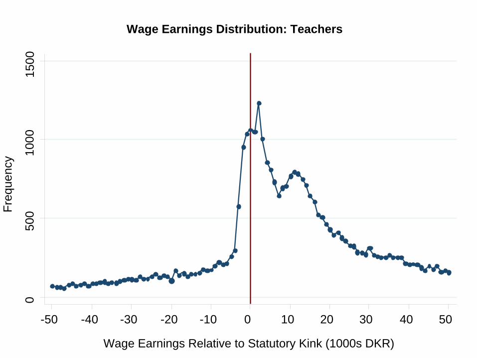
• Start with case study of one of the largest occupations: teachers
050
010
0015
00
-50 -40 -30 -20 -10 0 10 20 30 40 50
Wage Earnings Relative to Statutory Kink (1000s DKR)
Freq
uenc
y
Wage Earnings Distribution: Teachers

020
0040
0060
0080
0010
000
-50 -40 -30 -20 -10 0 10 20 30 40 50
Wage Earnings Relative to Statutory Kink (1000s DKR)
Freq
uenc
y Wage Earnings Distribution: Teachers with Deductions > DKr 20,000
This groupstarts paying top tax here
This groupstarts paying top tax here
This groupstarts paying top tax here

010
2030
-100 -50 0 50 100
Freq
uenc
y Modes of Occupation-Level Wage Earnings Distributions
Modes of Wage Earnings Distributions Relative to Top Bracket Cutoff (1000s DKr)

PREDICTION 2: Firm Responses and Small vs. Large Groups
• Prediction 2.1: There is firm bunching at the common kink
• Prediction 2.2: More firm bunching at more common kinks
• Compare between statutory and pension kinks
• Focus on group that faces neither kink:
• Deductions between 7,500 and 25,000

Wage Earnings Relative to Pension Kink (1000s DKR)
Freq
uenc
y Wage Earnings Around Pension Kink: Deductions > 20,000
2000
2500
3000
3500
4000
4500
-50 -40 -30 -20 -10 0 10 20 30 40 50
Excess mass (b) = 0.70Standard error = 0.20

Wage Earnings Relative to Pension Kink (1000s DKR)
Freq
uenc
y Wage Earnings Around Pension Kink: Deductions Between 7,500 and 25,000
2000
3000
4000
5000
-50 -40 -30 -20 -10 0 10 20 30 40 50
Excess mass (b)= -0.01Standard error = 0.15

Wage Earnings Relative to Statutory Kink (1000s DKR)
Freq
uenc
y Wage Earnings Around Statutory Kink: Deductions Between 7,500 and 25,000
2500
3000
3500
4000
4500
5000
-50 -40 -30 -20 -10 0 10 20 30 40 50
Excess mass (b)= 0.56Standard error = 0.10

PREDICTION 2: Firm Responses and Small vs. Large Groups
• Prediction 2.1: There is firm bunching at the common kink
• Prediction 2.2: More firm bunching at common kink
• Prediction 2.3: Larger observed elasticity at more common kinks
• Bunchers set wage earnings + deductions = top kink
• Need exogenous variation in deductions to isolate bunching through earnings margin
• Identification: Split pop. into gender-age-married-year groups
• Calculate fraction of each group with |net ded.| < 7500
• Use this group average as a proxy for how “common” is an individual’s level of deductions
• Calculate elasticity estimate from bunching for these groups

0.0
05.0
1.0
15.0
2.0
25
.45 .5 .55 .6 .65 .7Fraction of Group with |Net Deductions| < 7500
Obs
erve
d E
last
icity
from
Bun
chin
g at
Top
Kin
kObserved Elasticities vs. Scope of Tax Kink
Dynamics: Movement with the Kink
• Why do individuals move with the kink despite search frictions?
• Firm bunchers move with the kink because firm changes salaries for all workers
• Individual bunchers do not move with the kink because of search costs
Should see different individual bunchers at kink in each year
• Test by examining probability of tracking movement in kink
• Define indicator for change in earnings from year t to t+2 within DKr 7,500 of change in top tax bracket from t to t+2

2025
3035
-50 0-40 -30 -20 -10 10 20 30 40 50
% w
ith E
arni
ngs
Trac
king
Mov
emen
t in
Top
Kin
k
Wage Earnings Relative to Statutory Kink (1000s DKR)
Dynamics of Earnings Around the Statutory Kink

2025
3035
-50 0 50-40 -30 -20 -10 10 20 30 40
% w
ith E
arni
ngs
Trac
king
Mov
emen
t in
Pen
sion
Kin
k
Wage Earnings Relative to Pension Kink (1000s DKR)
Dynamics of Earnings around Pension Kink: Deductions > 20,000

PREDICTION 3: Correlation between Individual And Firm Bunching
• Intuitively, individual preferences drive the firm job distribution
• Test prediction by looking across occupations
• Two-digit Danish ISCO codes

Correlation between Individual and Firm Bunching
1
11
12
13
21
22
23
24
3132
33
34 4142
5152
61
71
72
73
74
8182
83
91
92
93
-20
24
68
-3 -2 -1 0 1 2 3 4
Firm
Bun
chin
g at
Top
Kin
k
Individual Bunching at Pension Kink
Correlation = 0.65 (p < 0.001)
1000
020
000
3000
040
000
5000
0
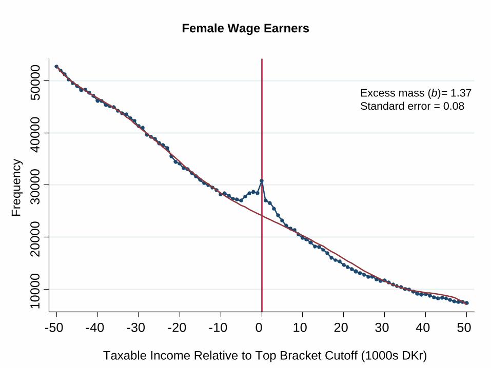
-50 -40 -30 -20 -10 0 10 20 30 40 50
Female Wage EarnersFr
eque
ncy
Taxable Income Relative to Top Bracket Cutoff (1000s DKr)
Excess mass (b)= 1.37Standard error = 0.08

Freq
uenc
y (U
nwei
ghte
d)
Freq
uenc
y (D
FL R
ewei
ghte
d)
Taxable Income Relative to Top Bracket Cutoff (1000s DKr)
Male Wage Earners
2000
030
000
4000
050
000
6000
010
000
2000
030
000
4000
050
000
6000
070
000
-50 -40 -30 -20 -10 0 10 20 30 40 50
DFL ReweightedExcess mass (b)= 0.85Standard error = 0.09
UnweightedExcess mass (b)= 0.46Standard error = 0.03

Self-Employed
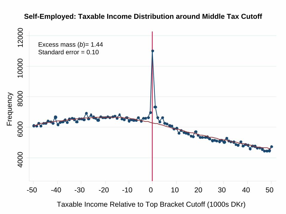
• Thus far, we have looked only at wage earners
• Self-employed do not face search frictions or hours constraints
• Can more easily adjust earnings, both by changing labor supply and by reporting/intertemporal shifting
• Serve as a “placebo test” for our findings
• Three predictions should not hold for the self-employed
• Size and scope of tax change should not matter

020
000
4000
060
000
-50 -40 -30 -20 -10 0 10 20 30 40 50
Excess mass (b) = 18.42Standard error = 0.42
Freq
uenc
y Self-Employed: Taxable Income Distribution around Top Tax Cutoff
Taxable Income Relative to Top Bracket Cutoff (1000s DKr)
4000
6000
8000
1000
012
000
-50 -40 -30 -20 -10 0 10 20 30 40 50
Excess mass (b)= 1.44Standard error = 0.10
Freq
uenc
y Self-Employed: Taxable Income Distribution around Middle Tax Cutoff
Taxable Income Relative to Top Bracket Cutoff (1000s DKr)

800
1000
1200
1400
1600
1800
-50 -40 -30 -20 -10 0 10 20 30 40 50
Excess mass (b)= 0.22Standard error = 0.47
Self-Employment Income Relative to Statutory Top Tax Cutoff (1000s DKr)
Freq
uenc
y Self-Employment Income Around Statutory Kink: Deductions > 20,000

0.1
.2.3
.4.5
.1 .2 .3 .4
Obs
erve
d E
last
icity
fro
m B
unch
ing
at T
op K
ink
Self-Employed: Observed Elasticities vs. Scope of Tax Changes
Fraction of Group with |Net Deductions| < 7500

Calibration
• What do our micro estimates tell us about the macro elasticity?
• Ideal experiment: Infinite tax change for a very small group
• Instead, we partially identify our model to bound the magnitude of the attenuation of the elasticity
• Key intuition: controls the utility loss of deviating from optimum
• Low implies very convex loss function, inflexible labor supply
Upper bound on utility losses from search cost yield a lower bound on the structural elasticity
uihi∗ − uih ≃ − 1
21 whi
∗Δ logh2

Calibration: Mechanics
• Calibrate tax system to match Danish economy
• Utility function:
• Fit heterogeneous tastes to match income distribution away from the kink
• Parametric assumptions:
Distribution of new draw:
Search cost:
• Fit the remaining parameters
from the data
uic,h c − i−1/ h 11/
11/
Geh ′ |hi∗ e lim
→0Nhi
∗, 1 − eNhi∗,
ie ci∗ 1 e

Excess Mass at the Top Kink vs. Search Costs
04
812
16
0 .1 .2 .3 .4 .5Structural Elasticity
Sim
ulat
ed E
xces
s M
ass
(b)
No frictions
= 0.04
= 0.06 Empirical Estimate

Excess Mass at the Middle and Top Kinks
Structural Elasticity Parameter
Sim
ulat
ed E
xces
s M
ass
(b)
01
23
45
6
0 .05 .1 .15 .2 .25 .3
= 0.06, Top Kink Empirical Estimate, Top Kink
= 0.06, Middle Kink Empirical Estimate, Middle Kink

Lower Bound on the Structural Elasticity
Average Utility Loss as a Fraction of Optimal Consumption ()
Low
er B
ound
on
Stru
ctur
al E
last
icity
()
0.1
.2.3
.4.5
.6
0 .02 .04 .06 .08 .1 .12

Simulated Equilibrium Income Distributions
No frictions With frictions
Income Relative to Top Bracket Cutoff
2000
060
000
1000
0014
0000
1800
00
Freq
uenc
y
-50 -40 -30 -20 -10 0 10 20 30 40 50

Conclusion
• Search costs and institutional constraints attenuate short run behavioral responses substantially
• Demonstrated the effects of size and scope on elasticity
• Standard method of estimating elasticities using small tax reforms on same data yields close-to-zero elasticity estimate
• If we assume utility loss from frictions is less than 5% of optimal consumption, 0.25 is a lower bound on consumption
• May help explain why macro cross-country comparisons find larger elasticities (Prescott 2004, Davis and Henrekson 2005)

Conclusion: Potential Policy Implications and Future Work
• Welfare consequences of tax policies can be very different in the presence of frictions
• Suppose individuals have heterogeneous elasticities and must coordinate on hours choices
long run efficiency cost of taxing one group of workers differs from that implied by their own elasticities
• Optimal taxation in the presence of frictions
• Effect of frictions on other behavioral responses and the interpretation of other quasi-experimental estimates

010
2030
40
100 200 300 400 500Income (1000 DKr)
Perceived Middle Tax Cutoff Perceived Top Tax Cutoff
Per
cent
of S
urve
y R
espo
nses
Survey Evidence on Knowledge About Middle and Top Tax Cutoffs