The Effect of Industrial Diversification on Firm Taxes

Kelly Wentland*

July 22, 2016

Abstract

This study investigates whether there is an empirical basis for one predicted benefit from industrial

diversification: whether conglomerate firms obtain greater tax savings than single industry firms.

The results suggest that, on average, firms operating in multiple industries incur lower tax

liabilities than stand-alone firms. However, whether a firm obtains these benefits is affected by the

type of industry-based tax positions available to the firm, the firm’s demand for debt, and its overall

risk strategy. For identification, the study uses a triple difference model based on two temporary

tax law changes and an instrumental variables analysis from the diversification discount literature.

Results from these tests are consistent with a tax advantage from diversification. Overall, the

results in the study inform recurring debates in the media and between management and

shareholders over the costs and benefits of diversification as a business strategy.

JEL classification: D23, H25, M40

Keywords: diversification, tax, organizational structure

* George Mason University, 4400 University Drive, Enterprise Hall, MS 1B1, Fairfax, VA 22030.

Email: kwentlan@gmu.edu. Phone: 703-993-5476. Fax: 703-993-1809. This study is based on my

dissertation completed at the University of North Carolina at Chapel Hill. I am grateful for input

from my dissertation committee: Ed Maydew (chair), Robert Bushman, Eva Labro, Jeremy

Moulton, and Doug Shackelford. In addition, I also appreciate helpful comments and suggestions

from Jeff Abarbanell, Kathleen Andries, Travis Dyer, Brad Hendricks, Robert Hills, Bret Johnson,

Sangwan Kim, Allison Koester, Martin Jacob, Mark Lang, Mark Ma, Jim Omartian, and Vivek

Raval. Finally, I thank the Accounting Doctoral Scholars Program for financial support and

AAA/Grant Thornton for selecting this dissertation for the Doctoral Dissertation Award for

Innovation in Accounting Education. All errors are my own.

1

I. INTRODUCTION

This study investigates whether diversified firms are able to achieve lower tax liabilities

than stand-alone firms.1 Proponents of industrial diversification often cite additional tax savings

as a key benefit from operating in multiple industries (Lewellen, 1971; Teece, 1980; Gertner,

Scharfstein, and Stein, 1994; Berger and Ofek, 1995; Furrer, 2011). The predicted tax advantage

comes from the expectation that diversified firms have less volatile streams of taxable income,

which reduces a firm’s exposure to tax convexity. Consistent with this, management at firms like

Berkshire Hathaway and General Electric have referenced additional tax benefits as one of the key

benefits of maintaining the conglomerate form. In his 2014 letter to shareholders, Warren Buffett

cited “important tax benefits” as one reason refocusing spin-offs “make no sense for us” at

Berkshire Hathaway (p. 33). Similarly, General Electric stated that concerns about losing tax

benefits from its financing operations business unit, GE Capital, deterred the decision to sell its

financing business for a long-time (The Wall Street Journal, April 13, 2015). Yet, despite

predictions for tax benefits (along with other argued advantages from operating in multiple

industries, such as synergies in operations and improved internal capital markets), the finance

literature more commonly documents that diversified firms trade at a discount or perform worse

relative to pure play firms (e.g., Lang and Stulz 1994; Berger and Ofek 1995; Laeven and Levine

2007; Humphery-Jenner 2013).

Despite this puzzle of the “diversification discount” in the valuation literature, there is

almost no empirical evidence directly testing whether the individual benefits of diversification

predicted in prior literature and practice are actually realized. As the diversification valuation

discount is only a puzzle if the assumptions about the proposed benefits of diversification are valid,

1 Throughout the study, I use the terms diversified firm, conglomerate, and multiple industry firm interchangeably

consistent with prior literature.

2

the purpose of this study is to examine one commonly held assumption – that industrial

diversification unambiguously creates tax benefits for firms.

I focus on the predicted tax advantage given the significant magnitude of the benefit

expected from this benefit. For example, Graham and Smith (1999) conclude that the average firm

in their analysis faces a convex tax function and that if firms can smooth pre-tax income volatility

by 5 percent then on average they can reduce expected tax liabilities by about 5.4 percent and in

extreme cases these savings can exceed 40 percent. In the case of General Electric’s decision to

sell its financing business (becoming less diversified), it projected a quick hit bringing a $6 billion

tax bill and an effective tax rate that could roughly double its previous rate (The Wall Street

Journal, April 13, 2015).

Using a broad sample of firms from 1999 through 2013, I begin with an investigation of

the average effect of diversification on firm tax liabilities. I find evidence supporting the prediction

that firms operating in multiple industries have lower tax liabilities than single industry firms on

average. Specifically, 25 percent of Compustat firms operate in multiple industries during my

sample period, and multiple industry firms in my sample obtain a 4.6 percentage point lower cash

effective tax rate (ETR) on average than firms operating in a single industry. This equates to $3.3

million of annual cash tax savings for the average firm in my sample. Results supporting the

average tax savings effect are robust to four measures of diversification.

In the next set of tests, I examine the extent to which factors predicted by prior literature

and practice moderate the potential tax benefits from diversification. Consistent with these

predictions, I find that a diversified firm does not obtain significant tax savings when tax benefits

from diversification are more likely to directly substitute for other industry-specific tax benefits,

or when a firm has less demand for additional debt (and resulting debt tax shields), relative to

3

single industry firms. Further, I find that firms following low to moderate risk strategies do not

observe additional tax benefits from diversification. These cross-sectional findings could at least

partially explain why we may observe differences in valuation effects across diversified firms.

My final set of tests are used to address concerns regarding potential endogeneity between

factors that may influence a firm’s choice to operate in multiple industries and its tax liabilities.

The first test examines two temporary tax law changes expected to alter the convexity of the tax

function and, therefore, tax benefits from diversification. Because temporary tax changes offer a

limited window in which firms can take advantage of the different tax benefits, it is unlikely firms

would suddenly (and temporarily) change the number of industries in which they operate to take

advantage of these tax law changes. The second test uses an instrumental variables approach

commonly used in the diversification discount literature aimed at addressing selection issues.

Using these alternate approaches, I find results consistent with my primary results, supporting the

prediction of a tax benefit from diversification.

This study contributes to the debate in the diversification literature and over the merits of

operational diversification as a firm business strategy. Prior literature predicts that there are many

potential benefits from diversification (Lewellen, 1971; Teece, 1980; Gertner, Scharfstein, and

Stein, 1994; Furrer, 2011), but generally provides evidence supporting a valuation discount or

underperformance for diversified firms overall when compared to single industry firms (Lang and

Stulz 1994; Berger and Ofek, 1995; Lins and Servaes, 1999; Rajan, Servaes, Zingales, 2000;

Scharfstein and Stein, 2000; Laeven and Levine, 2007; Humphery-Jenner, 2013). By documenting

tax savings related to diversification, this study is one of the first to offer empirical support to one

dimension used in assessing the specific merits of this business strategy. Further, by identifying

factors that moderate the tax benefits of diversification, I provide a tangible set of conditions for

4

why we may observe differences in valuation effects across diversified firms. While assessing the

valuation effect for the average firm is important, directly examining individual benefits and costs

of diversification (such as a firm’s tax benefit) may provide a greater set of tools for evaluating

why diversification has appeared to work for some firms (e.g., 3M and General Electric) but not

others (e.g. Time Warner’s attempt to establish an online presence with AOL and Quaker Oats’s

entry into the fruit juice market with Snapple). This approach suggests that a useful avenue for

future research could be the examination of other specific benefits (or costs) of diversification.

This topic is timely given recent high profile debates in the media over the merits and pitfalls of

diversification as a business strategy.2

In addition to contributions to the diversification literature, the results in this study suggest

that industrial diversification is also an important factor to consider in future research on firm tax

avoidance. While previous research demonstrates that the influence of other important factors (like

firm size) on taxes varies across industries (Zimmerman, 1983), studies in the literature generally

link a firm with its primary industry and do not account for whether it has operations in other

industries (e.g., Gupta and Newberry 1997; Rego 2003; Dyreng, Hanlon, and Maydew 2008; Chen,

Chen, Cheng, and Shevlin 2010; Armstrong, Blouin, and Larcker 2012). Researchers considering

only the primary industry in which a firm operates but not whether it operates in multiple industries

is analogous to considering that a firm is headquartered in the U.S. versus Ireland but not whether

it operates in multiple countries versus only domestically. Moreover, unlike certain determinants

of firm tax avoidance that require proprietary datasets (e.g., Robinson, Sikes, and Weaver 2010;

2 The business press points to a broad push by shareholders of conglomerates to refocus and discontinue operations

in sprawled out industries and, in response, management’s responding defense of the benefits of the conglomerate

form (The Wall Street Journal, January 25, 2016). Examples of firms that have faced this debate recently include

DuPont, Abbott Laboratories, Energizer, Tyco, and Johnson Controls (Reuters, September 17, 2014; Bloomberg,

March 1, 2015; The Wall Street Journal, August 9, 2015; The Wall Street Journal, January 25, 2016).

5

Armstrong, Blouin, and Larcker 2012), segment-based industry data is readily available in

Compustat and can be easily incorporated into future tax research as an important determinant of

a firm’s tax liabilities.

The remainder of the paper is organized as follows. Section 2 develops the hypothesis

tested in the study and describes related literature. Section 3 details the research design, sample,

and results for the primary analysis and cross-sectional tests. Section 4 re-examines the primary

analysis using two instrumental variables techniques. Section 5 concludes the study discussing

overall inferences and limitations.

II. HYPOTHESIS DEVELOPMENT AND RELATED LITERATURE

Diversifying through industry operations has been linked to several sources of tax benefits

in prior literature and practice. The first two predicted tax benefits from diversification come from

the literature linking hedging to income volatility. Smith and Stulz (1985) define hedging as both

the use of operational decisions (such as operating in multiple industries) and derivatives (or other

financial instruments) to reduce the covariance of streams of income with the state of the economy.

Smith and Stulz (1985) use a simple model of after-tax firm value to argue that if a firm’s tax

liability is a convex function of pre-tax income (i.e. the marginal tax rate is increasing with taxable

income), then by Jensen’s Inequality, companies that can reduce the volatility of their income

through hedging can obtain lower expected tax liabilities.3 Graham and Smith (1999) extend this

simplified analysis using simulation models to incorporate more realistic features of the tax code,

like tax loss carrybacks and carryforwards, investment tax credits, and the Alternative Minimum

3 To see why, consider an example from Graham and Rogers (2002). Assume a firm is equally likely to lose

$100,000 or earn $100,000 and that while profits are taxed at 35 percent, there is not an equivalent loss refund rate

(i.e. asymmetric tax treatment). Even though the expected income is zero, the firm expects to pay $17,500 in taxes.

If a firm can diversify its operations to smooth income volatility (with no difference to the expected income

amount), the firm then expects to pay zero dollars in tax. Thus, in this simple example, diversification generates

$17,500 of expected tax savings without altering the amount of expected taxable income for the firm.

6

Tax (AMT) and find that these features do not eliminate this benefit related to tax convexity but

rather extend the range of pre-tax income over which the convexity applies.4 Based on their

simulation analysis, Graham and Smith (1999) conclude that the average firm in their analysis

faces a convex tax function and that if firms can reduce their pre-tax income volatility by 5 percent

then on average they can reduce expected tax liabilities by about 5.4 percent.

The second tax benefit predicted from this literature results from implications of hedging

for optimal capital structure. Firms that hedge are expected to carry a lower risk of default and, as

a result, lending limits by creditors should be higher (Lewellen, 1971, Leland, 1998). Thus, firms

have the opportunity to trade-off risk that was not tax-favored (with more exposure to tax

convexity through volatile income streams in the absence of hedging) with tax-favored risk from

additional debt capacity, resulting in greater interest deductions and lower tax liabilities (Lewellen,

1971; Stulz, 1996; Leland, 1998). While these first two tax benefits may come from any form of

income volatility reduction or hedging, the third and fourth predicted tax benefits from

diversification are unique to operational forms of hedging (in this case, operating in multiple

industries) as opposed to hedging with derivatives.

These two operations-specific benefits relate to the firm’s ability to both use and uphold

tax positions. The tax code contains extensive provisions for tax benefits targeted at specific

industries.5 The dimension of industry for tax planning is also stressed by practice. For example,

all of the Big Four discuss advantages of industry specific knowledge about tax functions on their

4 They find that the primary institutional features affecting firm tax convexity are its tax loss carrybacks and

carryforwards. Practically speaking, tax loss carrybacks and carryforwards do not eliminate tax convexity primarily

because of the uncertainty of available taxable income to offset within the carryback and carryforward periods and

the time value of money (Majd and Myers, 1987). 5 One example is the Investment Credit, which consists of credits specific to coal, gasification, and energy projects

and the Credit for Increasing Research Activities (“R&D tax credit”) often linked to pharmaceutical, high tech, and

manufacturing industries. Other examples include specialized tax treatment for intangible drilling costs for oil and

gas companies and elections allowing the averaging/shifting of farm income over multiple tax years in agriculture.

7

websites.6 Yet, firms often face uncertainty about whether industry-specific tax benefits will

remain available, which can affect the extent to which they will use certain tax positions.7 Related

to this, the third tax benefit of industrial diversification is that, by operating in different industries,

a diversified firm may have a broader portfolio of tax planning opportunities and may not be as

sensitive to unfavorable changes to a single industry’s specific tax policies.

Another type of uncertainty that may limit a firm’s use of tax positions is its expectation

that whether, once a position is taken, it will be overturned by taxing authorities. The fourth benefit

of operating in multiple industries is that it may reduce both the likelihood of being audited and

the probability that, even if the firm is audited, the position will be overturned. This may result for

two reasons. First, firm taxes are often assessed by comparison with industry peers.8 9 In fact, the

Internal Revenue Service (IRS) has 52 Audit Technique Guides, which are primarily used to assist

its examiners assess unique tax and accounting methods of specific industries.10 When a firm

operates in different industries, it may be more difficult for a taxing authority to identify, for

example, an appropriate benchmark firm to flag whether the firm as having an abnormally low tax

liability or questionable estimates of tax benefits.11 Further, when a diversified firm does come

under audit, it may be more difficult for IRS examiners to evaluate the appropriate tax treatment

6 Deloitte: http://www2.deloitte.com/us/en/pages/tax/solutions/tax-services-by-industry.html; Ernst & Young:

http://www.ey.com/US/en/Industries; KPMG: http://www.kpmg.com/us/en/services/tax/pages/default.aspx;

http://www.kpmg.com/us/en/industry/pages/default.aspx; PricewaterhouseCoopers:

http://www.pwc.com/us/en/industrial-products/publications/2015-tax-rate-benchmarking-study.jhtml 7 For example, a last-minute bill in 2014 extended 54 corporate tax breaks (including specific tax breaks for banks,

the retail industry, and research and development) that corporations would have lost access to for their returns that

year (Huffington Post, December 16, 2014). 8 In a 2014 report on tax planning benchmarks, Pricewaterhouse Coopers explained that peer group comparisons,

which are often based on industry, provide opportunities in planning and shaping the tax function:

http://www.pwc.com/us/en/industrial-products/publications/2015-tax-rate-benchmarking-study.jhtml. 9 The IRS offers Industry Specific Tax Centers to provide businesses with specific guidance and analysis tools for

assessing their tax planning relative to their industry. 10 IRS Audit Technique Guides are available at: http://www.irs.gov/Businesses/Small-Businesses-&-Self-

Employed/Audit-Techniques-Guides-ATGs. 11 For example, it may difficult to identify an appropriate “tax peer” for companies that are diversified like 3M or

General Electric.

8

of a more complex organizational structure (e.g. understanding unique inter-industry transfer

pricing techniques available to multiple industry firms). Thus, by reducing uncertainty about both

available opportunities to reduce tax liabilities and the likelihood positions taken will be

overturned, diversified firms may be able to pay less in taxes than stand-alone firms. More broadly,

the fact that the IRS audits based on industry-specific guidelines should alert tax researchers to the

potential importance of investigating factors related to industries, and helps motivate the current

study from a practice standpoint.

Despite the potential for additional tax savings, there are at least four reasons diversified

firms may not obtain lower tax liabilities than stand-alone firms (or may even have higher tax

liabilities). First, the last benefit mentioned cuts both ways, in the sense that while it may be more

difficult for auditors to audit a multi-industry firm (given industry-specific tax code provisions), it

may also be more difficult or costly for firms to tax coordinate and plan for multiple industry

operations. Alternatively, stand-alone firms operating in a single industry may have a tax

department that is highly specialized, in a better position to know their industry’s tax provisions

inside and out, so-to-speak. Dating back as early as Adam Smith, the gains from specialization

have been well-established in economics, and there is no reason to believe that gains from

specialization should not apply to tax practitioners at large, publically traded companies. An

intuitive explanation of the tax cost for operating in multiple industries is simply that these firms’

tax departments are simply spread too thin, or less specialized, and therefore less adept at

maintaining tax rates as low as single-industry firms.12

Second, risk reduction is documented as an important motivator for diversification

(Amihud and Lev, 1981). Shareholders can achieve their own desired level of risk through

12 This viewpoint is consistent with the concerns about diverting management resources from the original focus of

operations expressed in Lynch and Rothchild (2000).

9

portfolio diversification and, thus, may have higher preference for the risk (and related returns)

from any single firm. Instead, managers often maintain a major portion of their total income from

their employment with a single firm through profit-sharing schemes, bonuses, and the value of

stock options. Given this, a risk-averse manager may opt for the conglomerate form as a means to

stabilize the firm’s streams of income, even if it is not valued by shareholders.13 As a result,

diversified firms may simply not take advantage of additional tax planning opportunities even if

they do exist (i.e. demonstrate no significant difference with stand-alone firms in terms of tax

savings) or may even choose to reduce tax benefits claimed if diversification is part of an overall

firm strategy to reduce risk (paying higher taxes than pure play firms).

Third, prior literature on derivatives and mergers and acquisitions (M&A) suggests firms

may not receive all of the specific, predicted tax benefits from other forms of hedging. Graham

and Rogers (2002) and Donohoe (2015) test the predictions from Graham and Smith (1999) that

there may be tax incentives to hedge through derivatives. While Graham and Rogers (2002) find

evidence consistent with greater interest tax shields from derivative use and Donohoe (2015) finds

evidence of additional tax benefits unique to transactions with derivatives, neither study finds

evidence that supports derivative use providing additional tax benefits from reduced tax convexity.

Further, in their multivariate analysis (Table 8), Devos, Kadapakkam, and Krishnamurthy (2009)

find no statistical difference between additional interest tax shields from diversifying mergers

(between acquirers and targets in different industries) versus focused mergers (between acquirers

and targets in the same industry). Overall, the results in these studies cast doubt on some of the

13 Amihud and Lev (1981) predict and find that the number of conglomerate mergers increases as the type of control

in the firm moves from strong shareholder control to weak shareholder control and then to management control. At

the same time, they find that the type of control does not appear to motivate non-conglomerate mergers, suggesting

that the diversification choice is not because of general growth in the firm. Further, May (1995) finds that firms with

CEOs that have more personal wealth vested in their firm’s equity tend to diversify firm operations.

10

individual tax benefit predictions from the general hedging and diversification specific literatures,

motivating a more general empirical examination of industrial diversification on taxes.

Finally, as mentioned in the introduction, while diversification is predicted to provide a

number of other non-tax benefits that are expected to generate greater firm value (in addition to

the tax benefits above), and a significant portion of firms continue to choose to operate in multiple

industries, generally the literature finds evidence that, on average, diversified firms are valued at

a discount or perform worse relative to stand-alone firms. This suggests that either firms are not

realizing these benefits in reality or that, even if these benefits are being accessed, additional costs

of the conglomerate form (which may have alternative tax consequences) offset these benefits for

shareholders. While the above alternative points suggest it may be reasonable to expect that

diversified firms claim no greater tax advantages than stand-alone firms, I state the following

hypothesis based on the greater tax benefit prediction (in the alternative form) given this is the

perspective focused on in the diversification literature:

H1: Diversified firms are able to obtain lower tax liabilities than stand-alone firms.

III. RESEARCH DESIGN, SAMPLE, AND RESULTS

Research Design

To examine H1, I employ variations of the following empirical model from the literature

on firm tax avoidance:

Taxi,t = β0 + β1 Diversificationi,t + ∑ β Controlsi,t + εi,t (1)

To measure a firm’s tax liabilities, Taxi,t,, I use a firm’s cash taxes paid scaled by the market

value of assets (Cash taxes paid/MVAi,t). Henry and Sansing (2015) document evidence that

scaling by the market value of assets helps address concerns about data truncation bias. Scaling by

this variable is particularly important for examining taxes in the setting of diversification for two

11

reasons. First, because effective tax rate (ETR)-based measures divide by pre-tax book income

reported in the financial statements, it only allows the measure to capture non-conforming (as

opposed to conforming) forms of tax avoidance (Hanlon and Heitzman, 2010). Conforming (non-

conforming) tax avoidance is a reduction in firm tax liability that affects a firm’s taxable income

and pre-tax book income in the same way (differing ways). Because ETR-based measures do not

capture conforming tax avoidance, it will not reflect tax benefits of interest deductibility (Hanlon

and Heitzman, 2010, p. 141) and potentially bias the results in a way relevant to this study’s

hypothesis.

In addition, ETR-based measures are generally not considered meaningful in years with

negative pre-tax income (Dyreng, Hanlon, and Maydew, 2008; Hope, Ma, and Thomas, 2013).14

As a consequence of this, studies using ETR measures generally exclude years with negative pre-

tax income from the analysis. This restriction is of particular concern in this study because one of

the predictions from the literature is that diversification is expected to reduce income volatility,

which may indicate that generally profitable diversified firms face less frequent exposure to loss

years than stand-alone firms. As a result, this truncation restriction for negative pre-tax income

years may affect diversified firms to a different extent than stand-alone firms and introduce a

systematic bias in the estimator.

The variable Cash taxes paid/MVAi,t is able to capture conforming tax avoidance and

allows inclusion of negative pre-tax income years because of the alternative scaling variable,

market value of assets. As explained in Hanlon and Heitzman (2010), a tax measure is able to

capture conforming tax avoidance if the conforming tax avoidance does not affect the numerator

14 For example, say a firm has negative pre-tax income and had negative cash taxes paid (i.e. a refund when it has a

loss). The ETR would be positive and potentially larger than for some firms that actually had positive pre-tax

income and cash taxes paid. Alternatively, a firm could have negative pre-tax income and positive taxes paid,

resulting in a negative ETR when taxes were actually paid.

12

and denominator of the tax measure in a way that preserves the value of the ratio without this

type of avoidance (they discuss this in the context of scaling by cash flows from operations as an

alternative to pre-tax book income in footnote 49).15 It is reasonable to expect that lower cash

taxes paid as a consequence of interest tax deductions would not affect the market value of assets

in such a way that it would maintain the same ratio in the absence of such benefits. Thus, I

expect this form of tax avoidance to be more likely to be captured in this alternate measure.

Further, the use of market value of assets prevents elimination of negative pre-tax income years

because it maintains a meaningful ratio in these years (since the denominator is still positive).16

The primary variable for Diversificationi,t is an indicator for whether a firm operates in

multiple industries (Multiple industriesi,t) similar to Berger and Ofek (1995) and prior literature on

diversification, taking the value of one when a firm operates in multiple industries and equaling

zero otherwise. In addition to Multiple industriesi,t, I examine three alternative proxies for

Diversificationi,t based on firm segment reporting: # of industriesi,t, % of sales in other industriesi,t,

and Sales-weighted distancei,t. The variables Multiple industriesi,t and # of industriesi,t follow from

the single versus multi-segment firm representation of diversification used in Berger and Ofek

(1995). The measure % of sales in other industriesi,t is based on the measure of multinational or

geographical diversification in Creal, Robinson, Rogers, and Zechman (2013), which uses the

percent of foreign sales as the extent of diversification. Sales-weighted distancei,t captures how

15 Hanlon and Heitzman (2010) discuss cash flow from operations as an alternative scaler to use to try and capture

conforming tax avoidance. However, cash flow does not as clearly eliminate the two concerns above for two

reasons. First, it is more reasonable to expect that interest expense and the related tax deduction would affect the

cash flow denominator and cash taxes paid in a way that preserves the tax variable ratio in the absence of this

expense/deduction than it is to expect that this ratio would be maintained in the presence of this tax benefit when

scaling by market value of assets. Further, scaling by cash flow from operations does not resolve the issue of

truncation with negative denominator values as cash flow is negative nearly as frequently as when pre-tax income is

negative. However, I do want to note that Hanlon and Heitzman (2010) do not offer the alternative cash flow scaling

variable as a suggestion for addressing the loss truncation issue. 16 See Henry and Sansing (2015) for a discussion of the motivation and validation of the alternate scaling variable in

addressing truncation bias in tax measures.

13

similar the segmented industries inside the firm are to the primary industry of the overall firm.

This measure is based on the “relatedness” measure used in Khorana, Shivdasani, Stendevad, and

Sanzhar (2011). I use a decile rank form of the latter two measures, % of sales in other industriesi,t

and Sales-weighted distancei,t. Based on H1 and the standard assumption in the diversification

literature, I expect to find that more diverse firms pay less taxes on average (i.e. a negative and

significant coefficient on Diversificationi,t (β1)).

Following prior literature on tax avoidance, I include an extensive set of control variables

to account for other tax planning opportunities, incentives, and common firm activities with

differences in book (financial accounting) and tax reporting that may affect firm taxes. The extent

of foreign operations (Foreign pre-tax incomei,t) and a firm’s decision to not disclose

disaggregated geographic earnings (No disclosurei,t) are associated with lower firm taxes (Rego,

2003; Hope, Ma, and Thomas, 2013). Larger firms may have greater economies of scale for tax

planning yet may draw greater attention from tax authorities and the public, generating mixed

predictions for the effect of firm size (Sizei,t) on firm taxes (Zimmerman, 1983; Gupta and

Newberry, 1997; Rego, 2003). Firms with additional leverage (Leveragei,t) may benefit from

additional debt tax shields. Available tax loss carryforwards (Tax Loss Carryforwardi,t) and

whether the firm has gathered (used) more of these carryforwards in the current period (Increase

in tax loss carryforwardi,t) can also affect firm taxes. Inclusion of controls for tax loss

carryforwards are particularly important in this setting because they may offset some of the

consequences of asymmetric tax treatment of income and losses.

More profitable firms (proxied by Pre-tax incomei,t) may have higher taxes simply because

of related higher taxable income. Yet, at the same time, these firms may have greater incentives

and resources to lower their taxes (Rego, 2003; Henry and Sansing, 2015). The remaining controls

14

represent firm activities that are treated differently for book and tax reporting purposes, which may

also affect firm taxes. Specifically, I inlcude controls for fixed assets (PP&E i,t), R&D and

intangibles intensity (R&Di,t and Intangiblesi,t), and the extent of earnings from unconsolidated

subsidiaries (Equity Incomei,t). Finally, following the prior literature on diversification, I include

firm (i) and year (t) fixed effects to account for other, unobserved, time-invariant factors across

firms (e.g. general firm business strategy) and other factors that may vary for all firms across time

(e.g. macroeconomic conditions or tax policy changes).17 18

Sample and Descriptive Statistics

The Compustat sample used for this study runs from 1999 to 2013. Statement of Financial

Accounting Standards No. 131 (SFAS 131) changed the requirements for segment reporting for

all fiscal years beginning after December 15, 1997. Because the diversification measures come

from business segment data, I begin the sample in 1999 to have consistent segment reporting

requirements throughout the entire sample period. I exclude firm-years with more than one

observation for a firm (e.g. a year when a firm changes its fiscal year-end). I then require non-

missing values for Cash taxes paid/MVAi,t, Multiple Industriesit, and the control variables

discussed in equation (1) as described in Appendix I. Similar to prior literature examining

diversification using segment data, and to ensure completeness of firm segment reporting for the

17Discussions in prior literature suggest that unobserved, time-invariant factors affecting a firm’s diversification

choice can influence the observed outcomes of diversification. A common approach to account for these factors in

the diversification literature is the inclusion of firm and year fixed effects in an OLS specification (Campa and

Kedia, 2002; Dimitrov and Tice, 2006; Lin, Pantzalis, and Park, 2007; Gopalan and Xie, 2011; Ammann, Hoechle,

and Schmid, 2012; and Hoechle, Schmid, Walter, and Yermack, 2012). Laeven and Levine (2007), Klein and

Saidenberg (2010), and Goetz, Laeven, and Levine (2013) focus on forms of diversification in financial institutions

and incorporate bank level fixed effects in their designs for the same purpose. I have also considered industry and

year fixed effects. However, this approach fails to account for factors that vary across firms within each industry,

which may bias inferences made with this analysis. Results with industry and year fixed effects differ. 18All of the studies applying the firm fixed effects model discussed in the prior footnote (except Goetz, Laeven, and

Levine (2013)) use two instrumental variable techniques developed in Campa and Kedia (2002) in conjunction with

their OLS fixed effects models to address endogeneity concerns. I perform analysis using these two alternate

techniques in Section 4.

15

diversification measures, I exclude firm-years where the sum of sales or assets across reported

segments deviated from the firm’s total sales or assets, respectively, by more than ten percent.19

The final sample has 26,910 firm-year observations.

Panel A of Table 1 reports descriptive statistics for the sample. The number of observations

differs for alternate measures of diversification, Return Volatilityi,t, and SA Indexi,t because these

continuous measures are not required for the primary sample, but are confined to the specific

analysis using these additional variables. The average Cash tax paid/MVAi,t of 0.0091 is analogous

to an average cash ETR of 0.32, which is consistent with the mean cash ETR values in prior tax

avoidance literature.20 Other summary statistics are also similar to those in prior literature.

Table 1 Panel B reports the descriptive statistics for the multiple industry and single

industry subsamples. Overall, firm-years with operations in multiple industries make up 20 percent

of the full sample. A few other descriptive statistics from this table are worth noting. Related to

specific predictions for taxes, on average, firms operating in multiple industries have higher Cash

tax paid/MVAi,t values but lower Leveragei,t. The higher Cash tax paid/MVAi,t and lower Leveragei,t

means for multiple industry firms provide preliminary evidence in contrast to the literature’s

predictions for tax benefits overall and for additional interest tax shields from diversification.

Consistent with the comparison of means, in an untabulated correlation matrix, the Pearson

(Spearman) correlations show a positive relation between Cash tax paid/MVAi,t and each of the

19 For example, Berger and Ofek (1995) and Campa and Kedia (2002) require non-missing segment data and

exclude observations where the sum of segment values of sales deviates from the Compustat annual total sales value

by one percent. In more recent studies, Ammann, Hoechle, and Schmid (2012) and Hoechle, Schmid, Walter, and

Yermack (2012) exclude observations where the sum of segment values of sales or assets deviates by five percent. I

use a ten percent threshold for this comparison to maintain as many observations as I can while still ensuring

completeness. The ten percent threshold for sales and assets is based on the ten percent threshold defining a

reportable segment in SFAS 131. Thus, if these values are within ten percent of the total (do not exceed a ten percent

deviation), I would not expect a reporting firm to be lacking a complete number of segments in that year. 20 The cash ETR value is calculated by multiplying Cash tax paid/MVAi,t with the average MVA for the sample

($2.5 billion) and dividing by the average pre-tax income for the sample ($71 million).

16

diversification measures, suggesting Diversificationi,t relates to paying higher taxes. At first

glance, this suggests that diversified firms may not have access to greater tax savings and may

even have higher tax liabilities. However, this observation is based on univariate analysis and does

not account for both observable and unobservable differences between firms applied in the later

multivariate tests. A final point on the correlation matrix is that the four proxies for diversification

are significantly and positively correlated as expected if these variables capture the same construct

(Pearson (Spearman) correlations ranging from 0.24-0.85 (0.46-0.99)).

OLS Results Using Alternative Measures of Diversification

The results for the OLS estimations of equation (1) are reported in Table 2. The different

columns in Table 2 use the aforementioned four alternative proxies for Diversificationi,t. Generally,

the control variables have the predicted associations with taxes from prior literature. For example,

I observe that firms with greater values of Leveragei,t and R&Di,t have lower values of Taxi,t. The

explanatory power of the estimated model for my sample is also reasonable in comparison with

recent tax avoidance studies using similar models.

With respect to H1, the prediction that diversified firms have lower tax liabilities than

stand-alone firms on average suggests that the coefficient on Diversificationi,t should be

significantly negative. Consistent with this, the coefficient on Diversificationi,t across all four

columns is negative and significant (t-statistics ranging from -1.92 to -2.35), indicating that

diversification is associated with paying lower tax liabilities.21

For ease of interpretation, I focus

on column (1) for discussion of economic magnitudes as this uses the primary measure of

Diversificationi,t in the literature. Based on column (1), I find that, on average, firms operating in

multiple industries have a 0.0013 lower Cash tax paid/MVAi,t than firms operating in a single

21 Results are robust to instead running a simplified firm and year fixed effects model excluding controls.

17

industry.22 At the sample average, this is analogous to a 4.6 percentage point lower cash ETR

associated with Diversificationi,t.23 In terms of comparable magnitudes, Gallemore and Labro

(2015) find that two of their proxies for internal information quality, the absence of a restatement

due to errors and lack of a Section 404 material weakness, are associated with 2 and 5 percentage

point reductions in cash ETR, respectively.

The results from Table 2 support the prediction in the diversification literature that

operating in multiple industries allows firms to claim greater tax savings. A natural question that

follows from this, then, is whether firms should assume that diversification will translate into

additional tax savings in all circumstances. In the next section, I consider three conditions that

could affect whether diversified firms are able to claim greater tax benefits from diversification.

Cross-sectional Tests

In this section, I investigate factors identified from prior literature or practice that could

moderate tax benefits from diversification. Identifying these factors may be helpful in assessing

why we observe variation in the valuation or performance effects of diversification across firms.

Research Design – R&D Activity

One way that diversification may not offer additional tax benefits to firms would be if the

additional potential tax benefits it produces directly reduce access to other forms of tax benefits

the firm would have as a single industry firm. For example, the General Business Credit (GBC) is

an aggregation of the R&D tax credit and 35 other Federal tax incentives, such as the investment

credit, enhanced oil recovery credit, renewable electricity production credit, and incentives for

22 Results throughout the study are robust to controlling for MVA. 23 The cash ETR interpretation for the average sample firm is calculated by multiplying the Cash tax paid/MVAi,t

coefficient with the average MVA for the sample (2,526) and dividing by the average pre-tax income for the sample

(71).

18

agricultural business.24 However, the aggregate GBC amount is limited to 75 percent of the

taxpayer’s net tax liability over $25,000. Thus, a firm that already has access to a large amount of

one type of industry credit (e.g. a large R&D tax credit) under the GBC may receive a muted tax

benefit from accessing other GBC incentives for other industries because it is more likely to

already meet the GBC tax benefit limitation. To consider this condition, the first test investigates

whether firms with greater levels of research and development (R&D) activity are less likely to

observe tax benefits from diversification.

I proxy for the potential tax benefit substitution effect with the extent of R&D activity a

firm has (R&Di,t), re-estimating equation (1) for partitions of low, moderate, and high R&D

activity. Specifically, I classify a firm as Low R&D (High R&D) if it has R&Di,t less than the 33rd

percentile (greater than the 67th percentile) for R&D active firms during the year.25 Firms with

R&Di,t between the 33rd and 67th percentile for R&D active firms during the year are classified as

Moderate R&D. I predict that if diversification offers distinct, industry-specific tax benefits, like

those listed in the GBC, then I should observe significant tax savings (should observe muted tax

savings) related to diversification when I expect a firm to have incremental (substitutable)

industry-based tax benefits from diversification as proxied by Low R&D (High R&D). Conversely,

if the tax benefit I observe on average is unrelated to industry-specific tax benefits like those in

the GBC, then I would be less likely to observe a difference in the diversification effect across the

high and low R&D partitions (as evidence of a substitution effect).

Research Design – Demand for Debt Capacity

Next, I examine whether firm demand for debt capacity affects the extent of tax benefits

from diversification. One source of tax benefits from diversification is predicted to follow from

24 For a comprehensive list of the other tax incentives, see IRC Sec. 38(b). 25 R&D active firms are considered those that have non-zero R&Di,t.

19

increased debt capacity and related interest deductions (Lewellen, 1971; Stulz, 1996; Leland,

1998). However, for diversification to generate tax benefits through this channel, a firm must

actually take advantage of additional debt financing. Thus, I expect that firms with greater (less)

demand for additional debt to be more likely to obtain greater (fewer) tax benefits from

diversification. I use whether a firm is financially constrained to proxy for its demand for additional

debt capacity.

Traditional pecking order theory suggests that firms prefer internal to external financing,

and then debt to equity financing, at least in part because of the high transaction costs of issuing

new securities (Myers, 1984; Fama and French, 2002). This model predicts that a firm’s use of

debt is driven by a firm’s net cash flows or financial constraints in that more financially constrained

firms are forced into using equity financing when they would otherwise prefer internal funds or

leverage. Based on this theory, I would expect that if diversification offers additional debt capacity

in general that financially constrained firms would be those most likely to take advantage of it (and

resulting debt tax shields).

I proxy for firm financial constraints using the SA indexi,t from Hadlock and Pierce (2010),

where higher values of the index represent greater financial constraint.26 I re-estimate equation (1)

for partitions of low, moderate, and high financial constraints. Specifically, I classify a firm as

having Low Constraints (High Constraints) if it has an SA index value less than the 33rd percentile

(greater than the 67th percentile) value for firms in the year it enters the sample. A firm with an SA

index between the 33rd and 67th percentile values in the year it enters the sample is classified as

having Moderate Constraints. I predict that if diversification offers firms additional debt capacity

and related interest tax shields then I should (should not) observe tax savings specifically related

26 See the detailed definition for the variable in Appendix I.

20

to diversification when firms are more highly (less) constrained.27 Conversely, if diversified firms

do not gain access to additional debt capacity (and related debt tax shields), I should not expect to

observe a different effect from diversification across the low and high constraint partitions.

Research Design – Firm Risk Preferences

Finally, recall the prediction that diversification may be part of a more general, firm

strategy or preference and that this may influence observed outcomes from diversification. In my

test for the on average effect (in Table 2), I attempt to control for unobserved, time invariant, firm

strategies by including firm fixed effects. However, in this last cross-sectional test, I instead focus

on teasing out one dimension of general firm strategy and how that affects the tax benefits observed

with diversification.28 Specifically, I consider tax outcomes related to diversification for firms with

different risk preferences.

Earlier in the study, I predicted that one reason I may not observe tax benefits from

diversification is because diversification may be part of a firm’s general low risk strategy where

these firms simply choose not to take advantage of additional tax savings even if they are available.

If this prediction holds, then I expect it to be less likely that I observe tax benefits from

diversification for firms following a low risk strategy. Conversely, if any additional tax savings

are available from diversification, I would expect a high risk firm to be the type of firm most likely

to claim these tax benefits.

27 This finding could also support an alternative explanation that is still linked to tax advantages of diversification,

just not the benefit of interest tax shields I outline specifically above. Law and Mills (2015) find that financially

constrained firms pursue more aggressive tax planning. Thus, based on the results of their study, if there are tax

advantages of diversification outside of additional debt capacity (without the firm demanding any additional debt), I

would also expect it to be more likely that financially constrained firms would tax advantage of those tax benefits

regardless of their use of additional leverage. 28 The results in my tests for the on average effect are robust to including the variable I use to proxy for firm risk

preference (return volatility) and the variable I use to proxy for demand for debt capacity (SA index) as well.

Equation (1) already includes the R&D variable (used for the first cross-sectional test) as a control.

21

To assess whether differences in firm risk influences observed tax benefits from

diversification, I use a common measure for firm risk, a firm’s Return volatilityi,t in the year it

enters the sample, and re-estimate equation (1) on partitions for low, moderate, and high risk

firms.29 Similar to the prior test partitioning on the SA index, I classify a firm as Low Risk (High

Risk) if it has return volatility less than the 33rd percentile (greater than the 67th percentile) value

for firms in the year it enters the sample. A firm with return volatility between the 33rd and 67th

percentile values in the year it enters the sample is classified as Moderate Risk.30

Results for Cross-sectional Tests

Results for the cross-sectional tests for firm R&D activity, demand for debt capacity, and

risk preference are reported in Tables 3-5, respectively. Columns (1)-(3) in each table report the

estimation of equation (1) for firms with low, moderate, and high values of the partitioning

variables, respectively. While I do not make specific predictions related to the moderate (middle)

columns, I include them for completeness.

The R&D test results in Table 3 show that for firms with low R&D activity (where I expect

the greatest potential for incremental, industry-specific, tax benefits from the GBC) Diversification

i,t has the predicted negative relation with firm tax liabilities (column (1): coefficient -0.0013, t-

statistic -2.11). Further, for firms with high R&D activity (those more likely to have a substitution

effect with the GBC) in (3), I do not find evidence of lower tax liabilities from diversification.

Specifically, the coefficient (t-statistic) on Diversificationi,t in this column is 0.0056 (1.58). A

cross-equation test indicates that the coefficient estimates of Diversificationi,t in columns (1) and

29 See the detailed definition for the variable in Appendix I.

30 A setting I considered but did not include in the cross-sectional analysis is the role of variation in corporate

governance on potential tax benefits from diversification. However, this set of cross-sectional tests is the focus of a

recent working paper Zheng (2015). Like Zheng (2015), I do not find evidence of differences in the diversification

effect across different proxies for corporate governance factors such as institutional ownership or insider ownership.

22

(3) (Low R&D and High R&D firms, respectively) are statistically different (2 = 16.50, p-value =

0.000).31 Overall, the results in Table 3 are consistent with incremental, industry-specific, tax

benefits contributing to the on average diversification tax benefit observed in Table 2.

In Table 4, I use the firm’s SA index value in the year it enters the sample as a measure of

demand for debt capacity. I only observe greater tax savings related to Diversificationi,t (a negative

association with firm tax liabilities) in the partition for firms with high financial constraints (with

the highest expected demand for debt capacity) (column (3): coefficient -0.0025, t-statistic -2.21).

For low constraint (demand) firms in columns (1), I do not find evidence of significant tax savings

for diversified firms. Specifically, the coefficient (t-statistic) on Diversificationi,t in this column is

-0.0001 (-0.15). A cross-equation test indicates that the coefficient estimates of Diversificationi,t

in columns (1) and (3) (Low Constraint and High Constraint firms, respectively) are statistically

different (2 = 11.13, p-value = 0.001). Thus, the results in Table 4 are consistent with firms

gaining access to greater debt capacity and related debt tax shields through diversification.

In Table 5, I use the firm’s return volatility in the year it enters the sample as a measure of

firm risk preference. I do not observe support for additional tax savings from diversification for

either low or moderate risk firms. Specifically, the coefficients (t-statistics) on Diversificationi,t in

this columns (1) and (2) are 0.0000 (0.04) and -0.0008 (-0.807), respectively. I only find greater

tax savings associated with Diversificationi,t (a negative association with firm tax liabilities) for

high risk firms (column (3): coefficient -0.0035, t-statistic -3.09). A cross-equation test indicates

that the coefficient estimates of Diversificationi,t in columns (1) and (3) (Low Risk and High Risk

firms, respectively) are statistically different (2 = 8.85, p-value = 0.003). The results in Table 5

31 I include the variable R&Di,t as a control for each partition to account for variation in R&D activity within the

partition. However, if I exclude this control and re-estimate each column, the sign, magnitude, and significance of

the coefficient on Diversificationi,t is very similar and do not change the inferences made above. For example, the re-

estimation for column (1) has a coefficient of -0.0014 and the t-statistic is -2.17.

23

suggest that firms diversifying, potentially as part of a low risk firm strategy, do not claim tax

benefits from diversification.

Overall, the results suggest that the primary tax benefits from diversification come through

industry specific tax provisions and debt tax shields. However, when the industry specific tax

provisions are more likely direct substitutes for other tax savings (such as within the GBC) or the

firm has less interest in taking advantage of additional tax-advantaged debt capacity, multiple

industry firms do not fare differently in terms of tax liabilities than single industry firms. Further,

diversified firms that follow a low or moderate business strategy do not access additional tax

savings from diversification. Taken together, this suggests that diversification does not always

offer firms additional tax savings and that whether these benefits are claimed is contingent on other

firm characteristics and strategies.

IV. ENDOGENEITY

The primary concern with endogeneity for my study would be if the firms selecting to

operate in multiple industries are those most likely to receive the benefits, which would indicate

that my results overstate tax benefits from diversification in general. In addition, there is always a

concern that a potential omitted correlated variable (or variables) may drive the results observed.

In this section, I use two additional tests in an attempt to address these concerns. The first test

examines two tax law changes expected to temporarily alter the convexity of the tax function and,

therefore, tax benefits from diversification. Because they are temporary tax changes with a limited

window for firms to take advantage of the different tax effects, it is less likely that firms would

suddenly (and temporarily) change the number of industries in which they operate to incorporate

the differences in the tax function. The second test uses an instrumental variables approach aimed

at addressing selection issues that is common in the diversification discount literature.

24

Triple Difference Model

As discussed before, the proposed tax benefits of diversification from the hedging

literature are grounded in the fact that the tax treatment of income and losses is asymmetric (i.e.,

a nonlinear convex structure). Thus, I would expect the incremental tax benefits of

diversification to vary when tax law changes occur that alter the convexity of the tax function.

Motivated by this, I consider whether the tax benefits of diversification were reduced for firms

affected by two tax law changes expected to reduce tax convexity during my sample period.

These tax law changes relate to temporary extensions of tax loss carrybacks.

An extended tax loss carryback period is expected to reduce the convexity of the tax

function. To see why, recall the original example from Graham and Rogers (2002) discussed in

the hypothesis section: assume a firm is equally likely to lose $100,000 or earn $100,000 and that

while profits are taxed at 35 percent, there is not an equivalent loss refund rate (i.e. asymmetric

tax treatment). Even though the expected income equals zero, the firm expects to pay $17,500 in

taxes. If a firm can diversify its operations to smooth income volatility (with no difference to the

expected income amount), the firm then expects to pay zero dollars in tax. In this simple

example, diversification generates $17,500 of expected tax savings without altering the amount

of expected taxable income for the firm.

Now instead, assume that the government enacts a tax law change that would allow the

firm to reclaim tax dollars paid on taxable income in previous years in the event it has the

$100,000 loss outcome in the current year. In this case, as long as the firm had sufficient taxable

income to offset in the years it carried the loss back to, the firm would receive a $35,000 refund

of prior year taxes paid in the loss outcome and the firm expects to pay on average zero dollars in

tax. In this latter regime, the predicted tax benefits of diversification in the hedging literature

25

disappear. A carryback period extension increases the likelihood a firm has enough taxable

income in the carryback period to offset a current year tax loss.32

A clear, direct test to investigate this convexity channel would be to observe an

exogenous tax law change (such as a carryback extension) that is assigned randomly to some

firms but not others. In the real world, however, tax law changes do not occur in a vacuum,

meaning that events surrounding the law change generally are related to the reasons the law is

enacted. While the presence of these surrounding events do not necessarily invalidate a test, it is

important to assess whether these events could bias a test in the direction of the predicted effect.

The U.S. federal government generally allows corporations a finite period to first

carryback losses for tax purposes and then carryforward remaining losses not offset in the

carryback period. 33 In two periods during my sample (1999-2013), the government temporarily

increased the window of years firms could carryback their losses to claim tax refunds from two

to five years (more than doubling the carryback period). However, this extension was only

applicable to firms that had net operating losses during specific calendar years (the group

receiving the “treatment”).

In the absence of a tax law change (the counterfactual), I would expect diversification to

produce greater tax benefits in periods of economic downturn precisely because of the tax

convexity channel. Tax asymmetry is most relevant when firms have volatile income,

32 Graham and Smith (1999) examine more realistic (complete) representations of the tax structure’s convexity that

incorporate several specific tax provisions. They find that provisions like tax loss carrybacks and carryforwards

significantly reduce the convexity of the tax code, but the impact of other provisions (like tax credits and the

alternative minimum tax) is minor. 33 Since the Taxpayer Relief Act of 1997 (prior to the start of my sample period), the U.S. Federal government has

generally allowed firms to carryback losses in this way two years and to carryforward any loss forward up to 20

years to offset future income if there is not sufficient taxable income to offset within the prior two year carryback

window. A carryback (carryforward) is generally considered more (less) beneficial as: 1) the firm knows whether it

will receive a benefit from the carryback (it knows how much taxable income it had in the past but does not know its

future taxable income) and 2) the related tax savings are an immediate refund (the present value of future tax savings

are discounted).

26

particularly when risk results in volatility that generates tax losses or lower taxable income

values (the convex region of the tax function), which is likely heightened in contractionary

periods. Thus, I predict that firms operating across multiple industries may suffer less from

market level volatility, face a less convex tax region, and therefore obtain greater tax savings

than single industry firms during these policy periods. However, if a carryback extension

becomes available for certain firms in those time periods, I would expect the additional tax

advantage of diversification during the economic downturn to be muted because the extension

reduces those firms’ exposure to tax convexity (even in the absence of a diversified operating

structure). Given that the period effect is expected to work in the opposite direction of the tax

law change effect (expected to generate greater tax savings related to diversification as opposed

to less), it is not clear how the events surrounding the law change bias toward my predicted

result. Thus, I use the temporary tax loss carryback tax law change setting to investigate the

convexity channel predicted in prior literature and for identification of my primary results.34

I use the following triple difference model (difference-in-difference-in-differences

(DDD)) to examine whether firms likely to be affected by these tax law changes observe muted

tax benefits of diversification during the affected tax policy periods:

Taxi,t = β0 + β1 Diversificationi,t + β2 Years Effectedt + β3 Eligible for Extensioni +

β4 Diversificationi,t x Years Affectedt + β5 Diversificationi,t x Eligible for Extensioni +

β6 Years Affectedt x Eligible for Extensioni + β7 Diversificationi,t x Years Affectedt x

Eligible for Extensioni + ∑ β Controlsi,t + εi,t (2)

34 This type of analysis is similar to how Card and Krueger (1994) examine the effect of minimum wage increases

on employment using New Jersey as eligible firms and Pennsylvania as ineligible firms and examining both sets of

firms both inside and outside the minimum wage policy change period. The minimum wage increase policy also

occurred during a recession, and the authors offer a similar sort of discussion as I do above for whether this is

expected to bias their findings.

27

where Taxi,t, Diversificationi,t, and Controlsi,t are defined as in equation (1).35 Eligible for

Extensioni is an indicator that varies across firms set equal to one if the firm is expected to be

eligible for the carryback extension within at least one of the law change periods and equals zero

otherwise. Years Affectedt is a time-varying indicator equal to one in years expected to be

affected by the law changes and equals zero otherwise.36 The primary coefficient of interest is

the coefficient on the triple interaction Diversificationi,t x Years Affectedt x Eligible for

Extensioni (β7). A significant, positive coefficient on β7 indicates that firms eligible for the

extension observed less tax benefits associated with diversification than other (ineligible) firms

in the years affected by the law change.

The results for equation (2) are reported in Table 6 Panel A and B. Panel A reports the

regression coefficients for equation (2). Consistent with the tax convexity channel prediction

above, the coefficient on the triple interaction is positive and significant at the 10 percent level

(coefficient 0.0015, t-statistic 1.84); firms eligible for the carryback extension observed less tax

benefits from diversification than ineligible firms during the extension carryback policy periods.

This finding is consistent with tax convexity as a channel driving the diversification tax benefit

and the carryback extension mitigating the benefit through this channel.

However, a more complete illustration of what is involved in this effect may be drawn

from walking through the matrix comparison in Panel B. This panel incorporates the results from

Panel A into a matrix comparing the effect of diversification across different categories of firms

and periods covered in equation (2). The rows distinguish the diversification effect on taxes

35 The only controls from equation (1) excluded are Tax loss carryforward it and Increase in tax loss carryforward it

because of the inclusion of the Eligible for Extensioni variable described in Appendix II, which is based on whether

the firm has tax loss carryforwards and changes in tax loss carryforwards. I also use industry and year fixed effects

(industry at the four digit SIC level) in place of firm and year fixed effects, requiring that there be multiple

observations of data available for each industry and year combination. 36 See Appendix I for detail on variable descriptions. See Appendix II for more institutional information on JCWAA

2002 and WHBAA 2009 in relation to these descriptions.

28

across time periods, and the columns distinguish the effect across groups of firms. The cell

representing the intersection of the difference column and row represents the incremental effect

from diversification on firm taxes while being in the eligible group within the affected policy

period after differencing out the time invariant differences across the two types of firms (eligible

and ineligible) and across the two periods (inside and outside the period affected).

Looking first at the differences across time periods (across the rows), diversification is

associated with greater tax savings (lower Taxi,t) inside the extension period relative to the period

outside the extension policies for ineligible firms but has no differential effect across periods for

eligible firms. Specifically, the difference coefficient is -0.0022 and significant at the 1 percent

level for ineligible firms and -0.0007 but not significant at conventional levels for eligible firms.

This is consistent with the prediction that contractionary periods may contain greater exposure to

the convex region of the tax function and that diversified firms weather this exposure more

favorably (for tax purposes) than single industry firms.

Looking then at the differences across groups of firms (across the columns), outside of

the period affected by the carryback there is not a statistical difference between the

diversification effect across the two groups (as shown by the 0.0010 coefficient that is

insignificant at conventional levels). However, inside the period affected, the eligible firms

appear to have less tax benefits from diversification than ineligible firms have (as shown by the

positive coefficient, 0.0025, significant at a 1 percent level). This suggests that the eligible firms

benefit less from diversification for tax purposes than ineligible firms inside the affected periods.

The positive, significant value at the intersection of the difference column and row (0.0015) is

the incremental effect of the extension policy on the eligible group, after accounting for time

invariant differences in the diversification effect between firm groups and across affected policy

29

periods. This is consistent with the extension policies applied to eligible firms mitigating tax

benefits from diversification through the tax convexity channel. Note that the 0.0015 coefficient

representing the intersection of the difference row and columns in Panel B is exactly the

coefficient on the triple interaction in Panel A.

As with all studies using a quasi-natural experiment in place of the ideal counterfactual

(i.e., the same firm subject to a tax policy in the absence of that policy), it is possible that the

criteria used to quality firms for a tax policy change could induce bias when estimating the effect

of that policy. In this test, the firms eligible for the carryback extension must have had a tax loss

in a certain time period. If a factor related to firms having a tax loss in this specific period (the

selection criteria) also relates to having higher taxes in the affected policy period than firms that

did not have a tax loss in the required period and were therefore ineligible for the policy, then this

may induce bias in the direction of the effect I observe and overstate the result.

Instrumental Variables Approach

Campa and Kedia (2002) use the fixed effects approach in my primary analysis and two

additional techniques using a simultaneous equation framework, a two-stage least squares (2SLS)

and treatment effects model (a form of selection model), to account for the endogeneity of a firm’s

diversification choice.37 To this end, I consider a set of firm, industry, and year level instruments

(Ii, t, k) for diversification proposed in Campa and Kedia (2002) in the following equations where:

Tax adjustedi,t = β0 + β1 Diversificationi,t + Σ β Controlsi,t, + εi,t (3)

Diversificationi,t = α0 + Σ α Ii,t,k + Σ α Controlsi,t + µi,t (4)

37 The approaches and instruments proposed in Campa and Kedia (2002) have been used frequently in the

diversification literature to address endogeneity concerns, including in the following studies: Dimitrov and Tice

(2006), Laeven and Levine (2007), Lin, Pantzalis, and Park (2007), Klein and Saidenberg (2010), Gopalan and Xie

(2011), Ammann, Hoechle, and Schmid (2012), Hoechle, Schmid, Walter, and Yermack (2012), and Hann, Ogneva,

and Ozbas (2013).

30

Following their study, I use two firm instruments to account for the ease with which a firm

can change between being diversified and focused in a single industry. Specifically, firms included

in the S&P Indexi,t and Listed on a Major Stock Indexi,t are expected to have greater visibility and

liquidity, making it easier to move between a diversified and focused structure. The time

instruments are proxies for business cycles, macroeconomic conditions, and merger waves.

Business cycles and macroeconomic conditions are captured by the concurrent and lagged # of

Contraction Months during the Yeart and % Change in Real GDPt. Merger waves are accounted

for by the Number of M&A Announced during the Yeart and Dollar Value of M&A Announced

during the Yeart. The two industry instruments represent the attractiveness of a given industry to

(potential) conglomerates. Specifically, the measures are the Fraction of Industry Firms that are

Multi-Industryi,t and the Fraction of Industry Sales from Multi-Industry Firmsi,t.38 See Appendix I

for additional detail on the variable definitions.

I use an adjusted tax variable as the outcome of interest, Tax adjustedi,t, which is demeaned

by firm and year. Campa and Kedia (2002) explain that by using an adjusted outcome variable in

this way the outcome variable is, by construction, uncorrelated with characteristics that affect the

outcome of interest on the adjustment dimensions (in this case, time invariant firm characteristics

and within year factors). As a result, they expect that, by construction, the instruments are unlikely

to be uncorrelated with εi,t. The authors conclude that given the variables above are expected to be

reasonable predictors of a firm’s diversification decision and are not expected to affect the outcome

of interest (in its adjusted form) directly, then the above set of variables are valid instruments for

38 I include one of the instruments used in Campa and Kedia (2002) in both equations (2) and (3) (i.e. use it as a

control in both equations rather than as an instrument). The variable is an indicator for whether a firm is

incorporated in a foreign country (Incorporated Outside the U.S.i,t). Given the prevalence of attention to

multinational tax planning, I include this variable in both stages as part of Xi,t to allow it to have both an indirect

effect on firm taxes through the firm’s diversification choice and a direct effect on taxes in the second stage.

31

this design.39 The remaining variables in equations (3) and (4) Diversificationi,t and Controlsi,t are

defined in the same way as for equation (1).

The results for the 2SLS and treatment effects approaches are reported in Table 7. For ease

of reference, I include the primary fixed effects OLS results from Table 2 in column (1) of Table

7 Panel A, given that these three methodologies are all commonly used in conjunction in the

literature.40 The estimates from equation (3) (equation (4)) are reported in Panel A (Panel B). When

comparing the results for my primary OLS specification with the results under these alternative

simultaneous equations approaches, the coefficients on Diversificationi,t in all three columns (for

all three approaches) are negative and significant, supporting a consistent tax benefit on average

from diversification across all three estimation approaches.

While I include the 2SLS and treatment effects models for completeness given their

prevalence in the literature, I express caution when relying on the instrumental variable test

inferences in place of the OLS results given the results of several diagnostic tests I examine related

to these tests. Wooldridge (2002) and Larcker and Rusticus (2010) recommend that researchers

applying an instrumental variables design use a series of diagnostic tests to assess the

appropriateness of the design for a specific research setting. Three tests they discuss are used to

assess the validity of the set of instruments: an F-test examining the null that the instruments do

not enter the first stage, an overidentification test of the null that the instruments are uncorrelated

with the error term in equation (3), and a review of an R-squared in a first-stage regression to

assess how well equation (4) explains the endogenous diversification choice. These tests of the

39 Larcker and Rusticus (2010) express concerns regarding the use of industry aggregates and lagged variables as

instruments. I cannot rule out the authors’ concerns for these variables with the aforementioned design. I include the

instrumental variable analysis for completeness as it has been used extensively in the diversification literature.

However, following the recommendations of Larcker and Rusticus (2010), in my analysis using this design I include

a series of diagnostic tests on the use of these instruments in my setting. I note the caveats or limitations related to

their concerns in the conclusions from this analysis below. 40 The 2SLS and treatment effects models are estimated with a maximum likelihood estimator.

32

validity of the instruments help assess whether the set of instruments: 1) are correlated with the

diversification choice after accounting for other predictor variables and 2) are uncorrelated with

the second stage residual. The final test is a Hausman test used to assess the null hypothesis that

the OLS fixed effect specification is a consistent estimator for Diversificationi,t under the

assumption that 2SLS is a consistent but inefficient estimator.

I report the results of the F-test, overidentification test, and the R-squared for the first stage

regressions in Table 7 Panel B. The Hausman test is untabulated but is discussed below. Overall,

the F-test and the R-squared related to the first stage regression provide some evidence that the set

of instruments are not weak in terms of their ability to predict a firm’s diversification choice.

However, the overidentification test suggests that it may not be valid to assume the instruments

should be excluded from the second stage. Furthermore, the Hausman test does not allow me to

reject the null of the exogeneity of Diversificationi,t in my primary OLS fixed effect specification

in comparision with the 2SLS estimator.

Specifically, the F-statistics (p-values) reported in Table 7 Panel B columns (1) and (2) are

2,627 (0.000) and 1,715 (0.000), respectively, vastly exceeding the statistic threshold for a weak

instrument suggested in Staiger and Stock (1997). 41 Further, the R-squared and pseudo R-squared

for the first stages reported in columns (1) and (2) of 0.210 and 0.214, respectively, suggest that

equation (3) explains a meaningful portion of the variation in Diversificationi,t overall. However,

the Hansen J Statistic for the overidentification test reported in Panel A for column (1) allows a

rejection of the null that the set of instruments are valid.42 Finally, a Hausman test comparing the

41 The F-test used comes from Bound, Jaeger, and Baker (1995) and Staiger and Stock (1997). These studies suggest

that the standard asymptotic approximations for instrumental variables breaks down when instruments are weak,

where they offer an F-statistic less than ten as an indication of when the instruments are weak. 42 The treatreg command in Stata does not support the overid post-estimation command, which is why I do not report

an overidentification test statistic for the treatment effects model. However, the same set of instruments and outcome

of interest are used in both the 2SLS and treatment effects models, suggesting the instruments would likely generate

a similar inference from an overidentification test for the treatment effects specification.

33

OLS fixed effects specification to the 2SLS specification (untabulated) does not allow me to reject

the null that the OLS fixed effects specification is a consistent estimator for my setting (p-value =

0.174) in comparison with the 2SLS estimation.

Overall, while the instrumental variables technique is commonly used to address

endogeneity concerns in the diversification literature, the results from the diagnostic tests in my

setting are mixed and do not allow me to rely solely on the instrumental variables approach to rule

out sources of endogeneity. To the extent that there are omitted factors not that cannot be ruled out

by inclusion of firm and year fixed effects in the OLS estimation and that are consistent with both

my cross-sectional tests and triple difference test results, my estimates may contain a source of

endogeneity bias not otherwise accounted for in the tests above.

V. CONCLUSION

An extensive line of academic research spanning multiple decades, along with debates in

practice, suggest that the value of corporate diversification as part of business strategy remains a

puzzle. This paper takes a unique approach to examining corporate diversification by focusing on

a specific, predicted benefit from this literature (namely, additional tax savings) rather than the

valuation effect overall. I find that, on average, firms operating in multiple industries have lower

tax liabilities than single industry firms. However, where the additional tax benefits from

diversification are expected to act as a substitute for tax positions already available, for firms that

do not face high financial constraints, or for firms without a high risk preference, I do not observe

significant additional tax savings related to diversification. The combined set of results here

provide greater understanding about the conditions under which a firm may obtain one of the key

cited benefits from industrial diversification. My results suggest an avenue for future research is

to examine other, specific benefits (or costs) from diversification (e.g. leveraging research and

34

innovation across multiple products and services) to inform the debate to help provide a greater

understanding of why we observe success related to diversification for some firms, but not others.

Like the diversification literature more generally, the results in this study are subject to an

important limitation. Ultimately, diversification is a strategy that firms decide whether or not to

employ that is not assigned randomly. Thus, it is difficult to rule out the possibility that there are

unobservable factors that relate to both this decision and firm tax liabilities. In this study, I attempt

to address this concern in multiple ways, such as incorporating firm and year fixed effects, a triple

difference model using tax policy changes, and two instrumental variable techniques from Campa

and Kedia (2002).

While it is always possible that an alternative factor is consistent with the combined results

from the techniques above, it is important to note that not all forms of potential endogeneity raise

concerns against the tax benefit result I observe. I offer this point not as a means to make light of

the concerns about the influence of endogeneity but to simply note that unless a specific factor or

source of endogeneity is identified that creates bias in the direction of my results, then it is unclear

whether potential endogeneity left unaccounted for in my design overstates as opposed to

understates the results I observe.

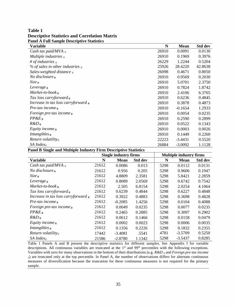
35

Table 1

Descriptive Statistics and Correlation Matrix Panel A Full Sample Descriptive Statistics

Variable N Mean Std dev

Cash tax paid/MVA it 26910 0.0091 0.0130

Multiple industries it 26910 0.1969 0.3976

# of industries it 26229 1.2244 0.5204

% of sales in other industries it 25926 28.4220 42.8638

Sales-weighted distance it 26098 0.4671 0.8050

No disclosure it 26910 0.9569 0.2030

Size it 26910 5.0701 2.3750

Leverage it 26910 0.7824 1.8742

Market-to-book it 26910 2.4106 6.3765

Tax loss carryforward it 26910 0.6236 0.4845

Increase in tax loss carryforward it 26910 0.3878 0.4873

Pre-tax income it 26910 -0.1654 1.2933

Foreign pre-tax income it 26910 0.0054 0.0235

PP&E it 26910 0.2590 0.2899

R&D it 26910 0.0522 0.1343

Equity income it 26910 0.0003 0.0026

Intangibles it 26910 0.1449 0.2260

Return volatilityit 22223 -3.4431 0.5520

SA Indexit 26884 -3.0092 1.1128

Panel B Single and Multiple Industry Firm Descriptive Statistics

Single industry firms Multiple industry firms

Variable N Mean Std dev N Mean Std dev

Cash tax paid/MVA it 21612 0.0086 0.013 5298 0.0112 0.0131

No disclosure it 21612 0.956 0.205 5298 0.9606 0.1947

Size it 21612 4.8809 2.3581 5298 5.8421 2.2859

Leverage it 21612 0.8089 2.0569 5298 0.6742 0.7542

Market-to-book it 21612 2.505 6.8154 5298 2.0254 4.1064

Tax loss carryforward it 21612 0.6239 0.4844 5298 0.6227 0.4848

Increase in tax loss carryforward it 21612 0.3922 0.4883 5298 0.3698 0.4828

Pre-tax income it 21612 -0.2085 1.4256 5298 0.0104 0.4088

Foreign pre-tax income it 21612 0.0049 0.0235 5298 0.0077 0.0235

PP&E it 21612 0.2465 0.2885 5298 0.3097 0.2902

R&D it 21612 0.0612 0.1466 5298 0.0158 0.0479

Equity income it 21612 0.0002 0.0023 5298 0.0006 0.0035

Intangibles it 21612 0.1356 0.2226 5298 0.1832 0.2355

Return volatilityit 17442 -3.4081 .5541 4781 -3.5709 0.5250

SA Indexit 21586 -2.8780 1.1342 5298 -3.5437 0.8285

Table 1 Panels A and B present the descriptive statistics for different samples. See Appendix I for variable

descriptions. All continuous variables are truncated at the 1st and 99th percentiles with the following exceptions.

Variables with zero for many observations in the bottom of their distributions (e.g. R&D it and Foreign pre-tax income

it) are truncated only at the top percentile. In Panel A, the number of observations differs for alternate continuous

measures of diversification because the truncation for these continuous measures is not required for the primary

sample.

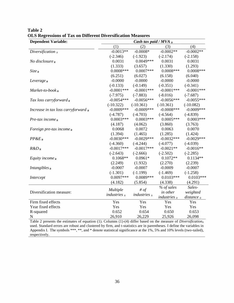
36

Table 2

OLS Regressions of Tax on Different Diversification Measures

Dependent Variable: Cash tax paid / MVA it

(1) (2) (3) (4)

Diversification it -0.0013** -0.0008* -0.0002** -0.0002**

(-2.346) (-1.923) (-2.174) (-2.158)

No disclosure it 0.0031 0.0049*** 0.0031 0.0031

(1.333) (3.657) (1.330) (1.293)

Size it 0.0008*** 0.0007*** 0.0008*** 0.0008***

(6.251) (6.027) (6.158) (6.040)

Leverage it -0.0000 -0.0000 -0.0000 -0.0000

(-0.133) (-0.149) (-0.351) (-0.341)

Market-to-book it -0.0001*** -0.0001*** -0.0001*** -0.0001***

(-7.975) (-7.883) (-8.016) (-7.687)

Tax loss carryforward it -0.0054*** -0.0056*** -0.0056*** -0.0055***

(-10.322) (-10.361) (-10.361) (-10.082)

Increase in tax loss carryforward it -0.0009*** -0.0009*** -0.0008*** -0.0009***

(-4.787) (-4.703) (-4.564) (-4.839)

Pre-tax income it 0.0003*** 0.0003*** 0.0005*** 0.0003***

(4.187) (4.062) (3.860) (3.763)

Foreign pre-tax income it 0.0068 0.0072 0.0063 0.0070

(1.394) (1.465) (1.285) (1.424)

PP&E it -0.0030*** -0.0029*** -0.0032*** -0.0029***

(-4.360) (-4.244) (-4.077) (-4.039)

R&D it -0.0017*** -0.0017*** -0.0021** -0.0016**

(-2.643) (-2.666) (-2.502) (-2.285)

Equity income it 0.1068** 0.0961* 0.1072** 0.1134**

(2.249) (1.932) (2.270) (2.239)

Intangibles it -0.0007 -0.0007 -0.0009 -0.0007

(-1.301) (-1.199) (-1.469) (-1.258)

Intercept 0.0097*** 0.0089*** 0.0103*** 0.0103***

(4.182) (5.854) (4.338) (4.291)

Diversification measure:

Multiple

industries it

# of

industries it

% of sales

in other

industries it

Sales-

weighted

distance it

Firm fixed effects Yes Yes Yes Yes

Year fixed effects Yes Yes Yes Yes

R-squared 0.652 0.654 0.650 0.653

N 26,910 26,229 25,926 26,098 Table 2 presents the estimates of equation (1). Columns (1)-(4) differ based on the measure of Diversificationit

used. Standard errors are robust and clustered by firm, and t-statistics are in parentheses. I define the variables in

Appendix I. The symbols ***, **, and * denote statistical significance at the 1%, 5% and 10% levels (two-tailed),

respectively.

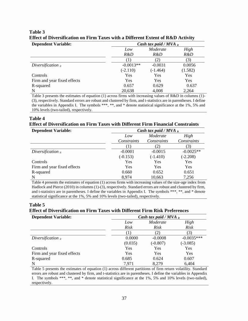
37

Table 3

Effect of Diversification on Firm Taxes with a Different Extent of R&D Activity

Dependent Variable: Cash tax paid / MVA it

Low

R&D

Moderate

R&D

High

R&D

(1) (2) (3)

Diversification it -0.0013** -0.0031 0.0056

(-2.110) (-1.464) (1.582)

Controls Yes Yes Yes

Firm and year fixed effects Yes Yes Yes

R-squared 0.657 0.629 0.637

N 20,638 4,008 2,264 Table 3 presents the estimates of equation (1) across firms with increasing values of R&D in columns (1)-

(3), respectively. Standard errors are robust and clustered by firm, and t-statistics are in parentheses. I define

the variables in Appendix I. The symbols ***, **, and * denote statistical significance at the 1%, 5% and

10% levels (two-tailed), respectively.

Table 4

Effect of Diversification on Firm Taxes with Different Firm Financial Constraints

Dependent Variable: Cash tax paid / MVA it

Low

Constraints

Moderate

Constraints

High

Constraints

(1) (2) (3)

Diversification it -0.0001 -0.0015 -0.0025**

(-0.153) (-1.410) (-2.208)

Controls Yes Yes Yes

Firm and year fixed effects Yes Yes Yes

R-squared 0.660 0.652 0.651

N 8,974 10,663 7,256 Table 4 presents the estimates of equation (1) across firms with increasing values of the size-age index from

Hadlock and Pierce (2010) in columns (1)-(3), respectively. Standard errors are robust and clustered by firm,

and t-statistics are in parentheses. I define the variables in Appendix I. The symbols ***, **, and * denote

statistical significance at the 1%, 5% and 10% levels (two-tailed), respectively.

Table 5

Effect of Diversification on Firm Taxes with Different Firm Risk Preferences

Dependent Variable: Cash tax paid / MVA it

Low

Risk

Moderate

Risk

High

Risk

(1) (2) (3)

Diversification it 0.0000 -0.0008 -0.0035***

(0.035) (-0.807) (-3.085)

Controls Yes Yes Yes

Firm and year fixed effects Yes Yes Yes

R-squared 0.685 0.624 0.607

N 7,971 8,279 6,404 Table 5 presents the estimates of equation (1) across different partitions of firm return volatility. Standard

errors are robust and clustered by firm, and t-statistics are in parentheses. I define the variables in Appendix

I. The symbols ***, **, and * denote statistical significance at the 1%, 5% and 10% levels (two-tailed),

respectively.

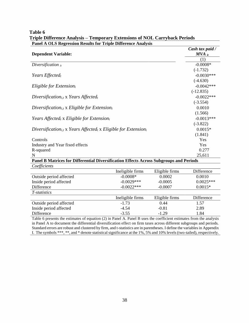
38

Table 6

Triple Difference Analysis – Temporary Extensions of NOL Carryback Periods

Panel A OLS Regression Results for Triple Difference Analysis

Dependent Variable:

Cash tax paid /

MVA it

(1)

Diversification it -0.0008*

(-1.732)

Years Effectedt -0.0030***

(-4.630)

Eligible for Extensioni -0.0042***

(-12.835)

Diversificationi,t x Years Affectedt -0.0022***

(-3.554)

Diversificationi,t x Eligible for Extensioni 0.0010

(1.566)

Years Affectedt x Eligible for Extensioni -0.0013***

(-3.822)

Diversificationi,t x Years Affectedt x Eligible for Extensioni 0.0015*

(1.841)

Controls Yes

Industry and Year fixed effects Yes

R-squared 0.277

N 25,611

Panel B Matrices for Differential Diversification Effects Across Subgroups and Periods

Coefficients

Ineligible firms Eligible firms Difference

Outside period affected -0.0008* 0.0002 0.0010

Inside period affected -0.0029*** -0.0005 0.0025***

Difference -0.0022*** -0.0007 0.0015*

T-statistics

Ineligible firms Eligible firms Difference

Outside period affected -1.73 0.44 1.57

Inside period affected -4.54 -0.81 2.89

Difference -3.55 -1.29 1.84 Table 6 presents the estimates of equation (2) in Panel A. Panel B uses the coefficient estimates from the analysis

in Panel A to document the differential diversification effect on firm taxes across different subgroups and periods.

Standard errors are robust and clustered by firm, and t-statistics are in parentheses. I define the variables in Appendix

I. The symbols ***, **, and * denote statistical significance at the 1%, 5% and 10% levels (two-tailed), respectively.

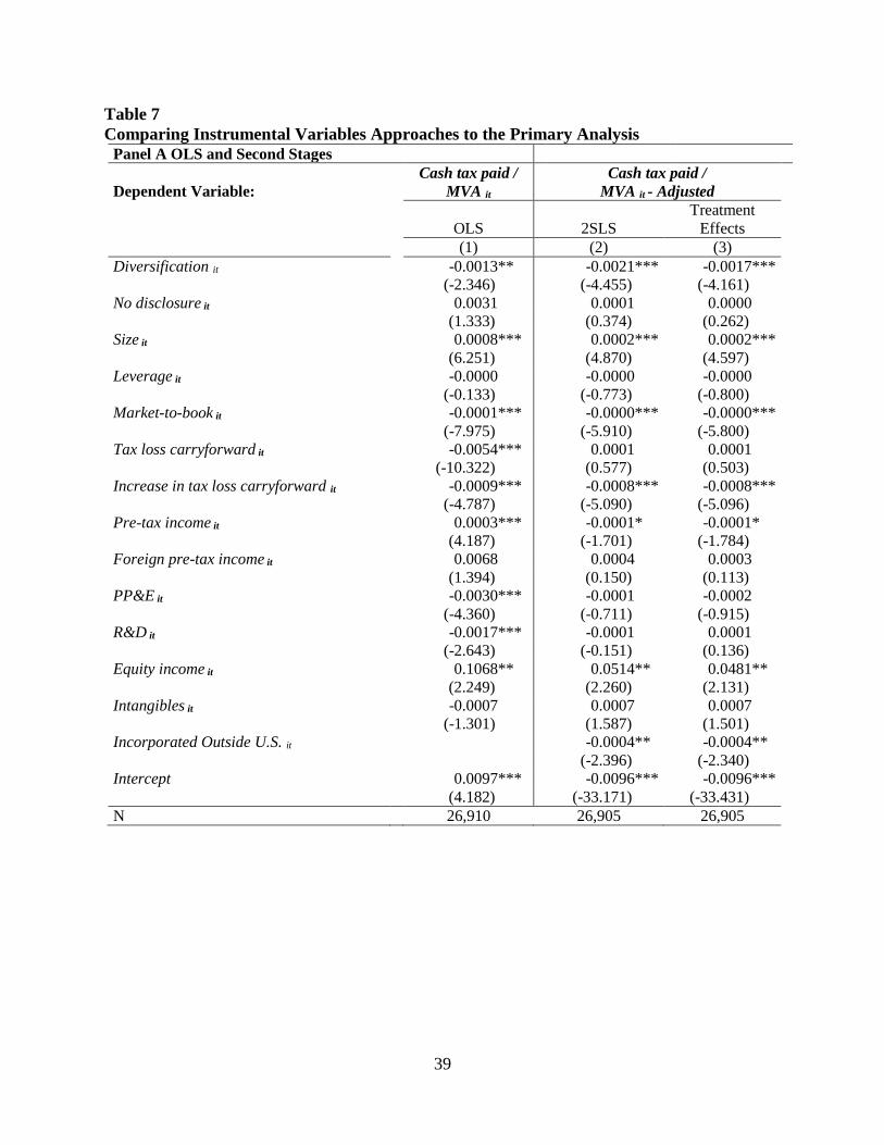
39

Table 7

Comparing Instrumental Variables Approaches to the Primary Analysis

Panel A OLS and Second Stages

Dependent Variable:

Cash tax paid /

MVA it

Cash tax paid /

MVA it - Adjusted

OLS 2SLS

Treatment

Effects

(1) (2) (3)

Diversification it -0.0013** -0.0021*** -0.0017***

(-2.346) (-4.455) (-4.161)

No disclosure it 0.0031 0.0001 0.0000

(1.333) (0.374) (0.262)

Size it 0.0008*** 0.0002*** 0.0002***

(6.251) (4.870) (4.597)

Leverage it -0.0000 -0.0000 -0.0000

(-0.133) (-0.773) (-0.800)

Market-to-book it -0.0001*** -0.0000*** -0.0000***

(-7.975) (-5.910) (-5.800)

Tax loss carryforward it -0.0054*** 0.0001 0.0001

(-10.322) (0.577) (0.503)

Increase in tax loss carryforward it -0.0009*** -0.0008*** -0.0008***

(-4.787) (-5.090) (-5.096)

Pre-tax income it 0.0003*** -0.0001* -0.0001*

(4.187) (-1.701) (-1.784)

Foreign pre-tax income it 0.0068 0.0004 0.0003

(1.394) (0.150) (0.113)

PP&E it -0.0030*** -0.0001 -0.0002

(-4.360) (-0.711) (-0.915)

R&D it -0.0017*** -0.0001 0.0001

(-2.643) (-0.151) (0.136)

Equity income it 0.1068** 0.0514** 0.0481**

(2.249) (2.260) (2.131)

Intangibles it -0.0007 0.0007 0.0007

(-1.301) (1.587) (1.501)

Incorporated Outside U.S. it -0.0004** -0.0004**

(-2.396) (-2.340)

Intercept 0.0097*** -0.0096*** -0.0096***

(4.182) (-33.171) (-33.431)

N 26,910 26,905 26,905

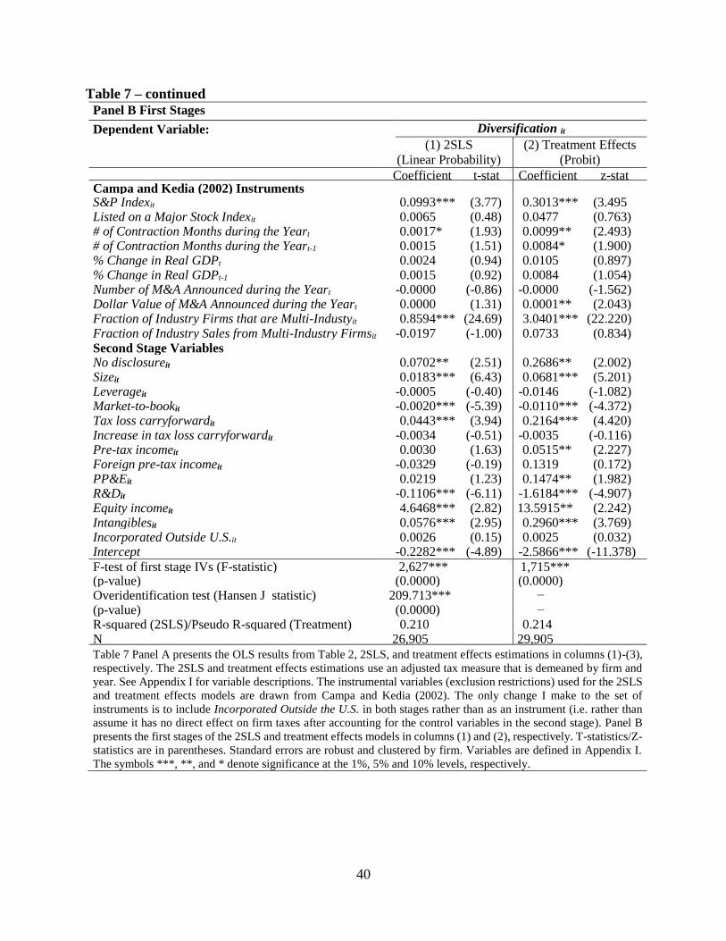
40

Table 7 – continued

Panel B First Stages

Dependent Variable: Diversification it

(1) 2SLS

(Linear Probability)

(2) Treatment Effects

(Probit) Coefficient t-stat Coefficient z-stat Campa and Kedia (2002) Instruments S&P Indexit 0.0993*** (3.77) 0.3013*** (3.495 Listed on a Major Stock Indexit 0.0065 (0.48) 0.0477 (0.763) # of Contraction Months during the Yeart 0.0017* (1.93) 0.0099** (2.493) # of Contraction Months during the Yeart-1 0.0015 (1.51) 0.0084* (1.900) % Change in Real GDPt 0.0024 (0.94) 0.0105 (0.897) % Change in Real GDPt-1 0.0015 (0.92) 0.0084 (1.054) Number of M&A Announced during the Yeart -0.0000 (-0.86) -0.0000 (-1.562) Dollar Value of M&A Announced during the Yeart 0.0000 (1.31) 0.0001** (2.043) Fraction of Industry Firms that are Multi-Industyit 0.8594*** (24.69) 3.0401*** (22.220) Fraction of Industry Sales from Multi-Industry Firmsit -0.0197 (-1.00) 0.0733 (0.834) Second Stage Variables No disclosureit 0.0702** (2.51) 0.2686** (2.002) Sizeit 0.0183*** (6.43) 0.0681*** (5.201) Leverageit -0.0005 (-0.40) -0.0146 (-1.082) Market-to-bookit -0.0020*** (-5.39) -0.0110*** (-4.372) Tax loss carryforwardit 0.0443*** (3.94) 0.2164*** (4.420) Increase in tax loss carryforwardit -0.0034 (-0.51) -0.0035 (-0.116) Pre-tax incomeit 0.0030 (1.63) 0.0515** (2.227) Foreign pre-tax incomeit -0.0329 (-0.19) 0.1319 (0.172) PP&Eit 0.0219 (1.23) 0.1474** (1.982) R&Dit -0.1106*** (-6.11) -1.6184*** (-4.907) Equity incomeit 4.6468*** (2.82) 13.5915** (2.242) Intangiblesit 0.0576*** (2.95) 0.2960*** (3.769) Incorporated Outside U.S.it 0.0026 (0.15) 0.0025 (0.032) Intercept -0.2282*** (-4.89) -2.5866*** (-11.378)

F-test of first stage IVs (F-statistic) 2,627*** 1,715*** (p-value) (0.0000) (0.0000) Overidentification test (Hansen J statistic) 209.713*** − (p-value) (0.0000) − R-squared (2SLS)/Pseudo R-squared (Treatment) 0.210 0.214 N 26,905 29,905

Table 7 Panel A presents the OLS results from Table 2, 2SLS, and treatment effects estimations in columns (1)-(3),

respectively. The 2SLS and treatment effects estimations use an adjusted tax measure that is demeaned by firm and

year. See Appendix I for variable descriptions. The instrumental variables (exclusion restrictions) used for the 2SLS

and treatment effects models are drawn from Campa and Kedia (2002). The only change I make to the set of

instruments is to include Incorporated Outside the U.S. in both stages rather than as an instrument (i.e. rather than

assume it has no direct effect on firm taxes after accounting for the control variables in the second stage). Panel B

presents the first stages of the 2SLS and treatment effects models in columns (1) and (2), respectively. T-statistics/Z-

statistics are in parentheses. Standard errors are robust and clustered by firm. Variables are defined in Appendix I.

The symbols ***, **, and * denote significance at the 1%, 5% and 10% levels, respectively.

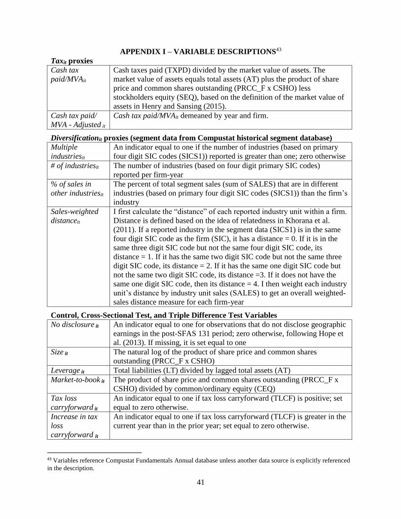
41

APPENDIX I – VARIABLE DESCRIPTIONS43

Taxit proxies

Cash tax

paid/MVAit

Cash taxes paid (TXPD) divided by the market value of assets. The

market value of assets equals total assets (AT) plus the product of share

price and common shares outstanding (PRCC_F x CSHO) less

stockholders equity (SEQ), based on the definition of the market value of

assets in Henry and Sansing (2015).

Cash tax paid/

MVA - Adjusted it

Cash tax paid/MVAit demeaned by year and firm.

Diversificationit proxies (segment data from Compustat historical segment database)

Multiple

industriesit

An indicator equal to one if the number of industries (based on primary

four digit SIC codes (SICS1)) reported is greater than one; zero otherwise

# of industriesit The number of industries (based on four digit primary SIC codes)

reported per firm-year

% of sales in

other industriesit

The percent of total segment sales (sum of SALES) that are in different

industries (based on primary four digit SIC codes (SICS1)) than the firm’s

industry

Sales-weighted

distanceit

I first calculate the “distance” of each reported industry unit within a firm.

Distance is defined based on the idea of relatedness in Khorana et al.

(2011). If a reported industry in the segment data (SICS1) is in the same

four digit SIC code as the firm (SIC), it has a distance = 0. If it is in the

same three digit SIC code but not the same four digit SIC code, its

distance = 1. If it has the same two digit SIC code but not the same three

digit SIC code, its distance = 2. If it has the same one digit SIC code but

not the same two digit SIC code, its distance =3. If it does not have the

same one digit SIC code, then its distance = 4. I then weight each industry

unit’s distance by industry unit sales (SALES) to get an overall weighted-

sales distance measure for each firm-year

Control, Cross-Sectional Test, and Triple Difference Test Variables

No disclosure it An indicator equal to one for observations that do not disclose geographic

earnings in the post-SFAS 131 period; zero otherwise, following Hope et

al. (2013). If missing, it is set equal to one

Size it The natural log of the product of share price and common shares

outstanding (PRCC_F x CSHO)

Leverage it Total liabilities (LT) divided by lagged total assets (AT)

Market-to-book it The product of share price and common shares outstanding (PRCC_F x

CSHO) divided by common/ordinary equity (CEQ)

Tax loss

carryforward it

An indicator equal to one if tax loss carryforward (TLCF) is positive; set

equal to zero otherwise.

Increase in tax

loss

carryforward it

An indicator equal to one if tax loss carryforward (TLCF) is greater in the

current year than in the prior year; set equal to zero otherwise.

43 Variables reference Compustat Fundamentals Annual database unless another data source is explicitly referenced

in the description.

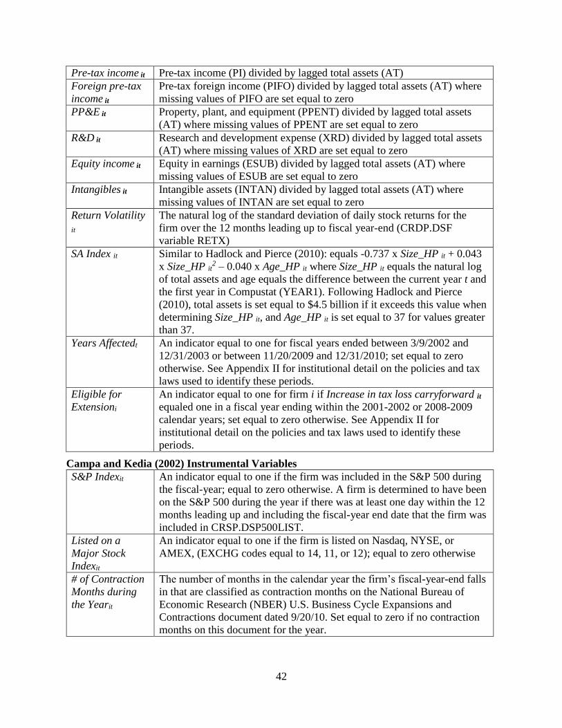
42

Pre-tax income it Pre-tax income (PI) divided by lagged total assets (AT)

Foreign pre-tax

income it

Pre-tax foreign income (PIFO) divided by lagged total assets (AT) where

missing values of PIFO are set equal to zero

PP&E it Property, plant, and equipment (PPENT) divided by lagged total assets

(AT) where missing values of PPENT are set equal to zero

R&D it Research and development expense (XRD) divided by lagged total assets

(AT) where missing values of XRD are set equal to zero

Equity income it Equity in earnings (ESUB) divided by lagged total assets (AT) where

missing values of ESUB are set equal to zero

Intangibles it Intangible assets (INTAN) divided by lagged total assets (AT) where

missing values of INTAN are set equal to zero

Return Volatility

it

The natural log of the standard deviation of daily stock returns for the

firm over the 12 months leading up to fiscal year-end (CRDP.DSF

variable RETX)

SA Index it Similar to Hadlock and Pierce (2010): equals -0.737 x Size_HP it + 0.043

x Size_HP it2 – 0.040 x Age_HP it where Size_HP it equals the natural log

of total assets and age equals the difference between the current year t and

the first year in Compustat (YEAR1). Following Hadlock and Pierce

(2010), total assets is set equal to $4.5 billion if it exceeds this value when

determining Size_HP it, and Age_HP it is set equal to 37 for values greater

than 37.

Years Affectedt An indicator equal to one for fiscal years ended between 3/9/2002 and

12/31/2003 or between 11/20/2009 and 12/31/2010; set equal to zero

otherwise. See Appendix II for institutional detail on the policies and tax

laws used to identify these periods.

Eligible for

Extensioni

An indicator equal to one for firm i if Increase in tax loss carryforward it

equaled one in a fiscal year ending within the 2001-2002 or 2008-2009

calendar years; set equal to zero otherwise. See Appendix II for

institutional detail on the policies and tax laws used to identify these

periods.

Campa and Kedia (2002) Instrumental Variables

S&P Indexit An indicator equal to one if the firm was included in the S&P 500 during

the fiscal-year; equal to zero otherwise. A firm is determined to have been

on the S&P 500 during the year if there was at least one day within the 12

months leading up and including the fiscal-year end date that the firm was

included in CRSP.DSP500LIST.

Listed on a

Major Stock

Indexit

An indicator equal to one if the firm is listed on Nasdaq, NYSE, or

AMEX, (EXCHG codes equal to 14, 11, or 12); equal to zero otherwise

# of Contraction

Months during

the Yearit

The number of months in the calendar year the firm’s fiscal-year-end falls

in that are classified as contraction months on the National Bureau of

Economic Research (NBER) U.S. Business Cycle Expansions and

Contractions document dated 9/20/10. Set equal to zero if no contraction

months on this document for the year.

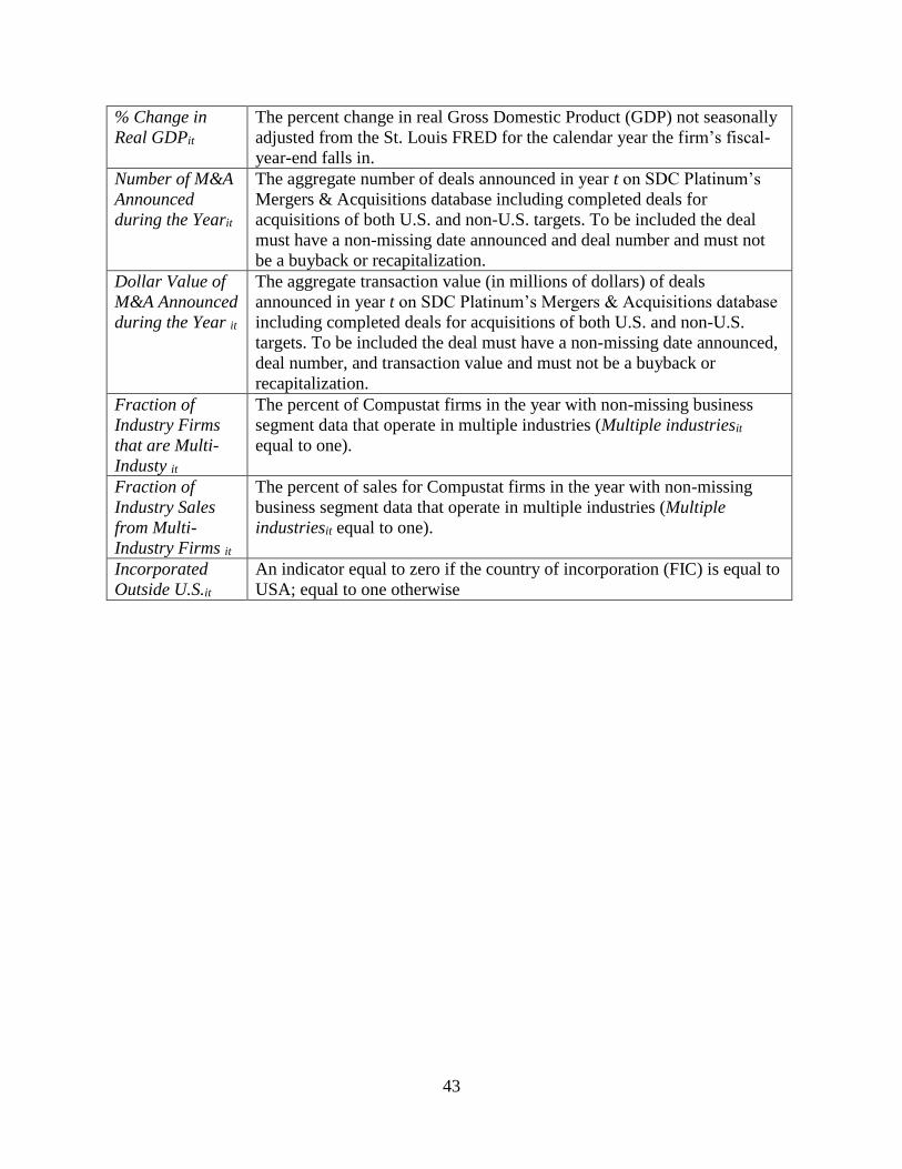
43

% Change in

Real GDPit The percent change in real Gross Domestic Product (GDP) not seasonally

adjusted from the St. Louis FRED for the calendar year the firm’s fiscal-

year-end falls in.

Number of M&A

Announced

during the Yearit

The aggregate number of deals announced in year t on SDC Platinum’s

Mergers & Acquisitions database including completed deals for

acquisitions of both U.S. and non-U.S. targets. To be included the deal

must have a non-missing date announced and deal number and must not

be a buyback or recapitalization.

Dollar Value of

M&A Announced

during the Year it

The aggregate transaction value (in millions of dollars) of deals

announced in year t on SDC Platinum’s Mergers & Acquisitions database

including completed deals for acquisitions of both U.S. and non-U.S.

targets. To be included the deal must have a non-missing date announced,

deal number, and transaction value and must not be a buyback or

recapitalization.

Fraction of

Industry Firms

that are Multi-

Industy it

The percent of Compustat firms in the year with non-missing business

segment data that operate in multiple industries (Multiple industriesit

equal to one).

Fraction of

Industry Sales

from Multi-

Industry Firms it

The percent of sales for Compustat firms in the year with non-missing

business segment data that operate in multiple industries (Multiple

industriesit equal to one).

Incorporated

Outside U.S.it

An indicator equal to zero if the country of incorporation (FIC) is equal to

USA; equal to one otherwise

44

APPENDIX II – TAX CARRYBACK EXTENSIONS

Within my sample period, the U.S. Federal government temporarily expanded the tax loss

carryback period twice. The first occurrence was part of the Job Creation and Worker Assistance

Act of 2002 (JCWAA 2002) enacted on March 9, 2002, which offered firms with net operating

losses (NOLs) for tax years ending in 2001 and 2002 the opportunity to carryback their NOLs

against the five prior tax years’ taxable income as opposed to only a two year carryback period

(Public Law 107-147). The second expansion resulted from the Worker, Homeownership, and

Business Assistance Act of 2009 (WHBAA 2009) signed into law on November 20, 2009, which

offered firms with NOLs for tax years ending in 2008 or 2009 the option to carryback their tax

loss up to five years (Revenue Procedure 2009-52). Thus, the first steps in an analysis of how

these two tax changes influenced the diversification effect for firm taxes is to:

1) Identify the “treatment” group of firms that are more likely to be affected by these

carryback period extensions (define Eligible for Extensioni).

2) Distinguish the periods when the treatment firms accessing the cash taxes paid benefit

from these extensions would show up in their financial statements (Years Affectedt).

In order for the extension to apply, a firm would have had NOLs in the periods of

eligibility that would not have otherwise been carried back (used up) in the absence of the

carryback extension. I therefore proxy for whether a firm is more likely to be eligible for the

extension based on whether a firm had an increase in tax loss carryforwards for at least one fiscal

year ending in the periods of eligibility (2001-2002 or 2008-2009).44 I label this variable,

44 Generally, NOLs that are not carried back (either because there is not sufficient taxable income to offset or

because a firm elects to opt out of using an NOL carryback) are carried forward to be applied against future taxable

income. Thus, I assume that additional NOLs available for carryback extension manifest as an increase to NOL

carryforward in the relevant policy year.

45

Eligible for Extensioni, which is set equal to one for a firm that had an increase in the periods and

is set equal to zero otherwise.

To determine Years Affectedt, I needed to identify a window of time starting with the

earliest fiscal year end that could reflect the additional tax refunds from the extension policies

(via Cash tax paid/MVAit) up through the latest fiscal year end that likely reflects these refunds.

For the beginning of each of the two policy windows, I use the dates of enactment for the two

extension policies (for JCWAA 2002 and WHBAA 2009, I use March 9, 2002 and November

20, 2009, respectively).45 The end of each window is based on IRC Sec. 6411(a), which allows a

firm to file an application for carryback adjustment for the prior taxable year affected by a NOL

carryback within 12 months after that tax year ends. Thus, the relevant ending window used for

each policy is 12 months after the end of the eligible NOL period for each policy (12 months

after the 2001-2002 eligibility period for JCWAA 2002 is December 31, 2003 and 12 months

after the 2008-2009 eligibility period period for WHBAA 2009 is December 31, 2010).46 I

therefore set Years Affectedt equal to one for fiscal years ending between March 9, 2002 and

December 31, 2003 and between November 20, 2009 and December 31, 2010.

45 WHBAA 2009 is actually an expansion of the American Recovery and Reinvestment Act of 2009 signed into law

on February 17, 2009, which only allowed the extended carryback period to “eligible small firms” to most other

businesses (Public Laws 111-5 and 107-147). Given that less than 17 percent of my sample have book sales less

than the eligible small firm threshold, I use the November 20, 2009 date for my primary period start date. However,

if I re-run my triple difference analysis using the February start date, the result for the triple interaction actually has

greater statistical significance (is positive and significant at the 5 percent level instead of the 10 percent level). 46 There may be some portion of firms that both have their tax year ends at the very end of the eligibility period and

file their carryback adjustment request at the tail end of the 12 month window after the eligibility period ends where

the refund recognized could bleed into the period following what is labeled Years Affectedt equal to one. However,

this should make it harder to find the effect in the window examined by pulling part of the effect into the benchmark

period (outside the affected period).

46

REFERENCES

Amihud, Y. and Lev, B. 1981. Risk Reduction as a Managerial Motive for Conglomerate

Mergers. Bell Journal of Economics 12: 605-617.

Ammann, M., Hoechle, D., and Schmid, M. 2012. Is there Really No Conglomerate Discount?

Journal of Business Finance & Accounting 39(1) & (2):264-288.

Armstrong, C., Blouin, J., and Larcker, D. 2012. The incentives for tax planning. Journal of

Accounting and Economics 53(1-2): 391-411.

Benoit, D. and Grind, K. August 9, 2015. Activist Investors’ Secret Ally: Big Mutual Funds:

Large Investors quietly back campaigns to force change at U.S. companies. The Wall Street

Journal. < http://www.wsj.com/articles/activist-investors-secret-ally-big-mutual-funds-

1439173910>

Berger, P. and Ofek, E. 1995. Diversification’s effect on firm value. Journal of Financial

Economics 37: 39-65.

Bound, J., Jaeger, D., and Baker, R. 1995. Problems with Instrumental Variables Estimation

when the Correlation between the Instruments and the Endogenous Explanatory Variable is

Weak. Journal of the American Statistical Association 90(430): 443-450.

Campa, J. M. and Kedia, S. 2002. Explaining the Diversification Discount. Journal of Finance.

57(4): 1731-1762.

Chen, S., Chen, X., Cheng, Q., and Shevlin, T. 2010. Are family firms more tax aggressive than

non-family firms? Journal of Financial Economics 95: 41-61.

Creal, D., Robinson, L, Rogers, J., and Zechman, S. 2014. The Multinational Advantage.

University of Chicago working paper No. 11-37.

Devos, E., Kadapakkam, P.R. and Krishnamurthy, S. 2009. Review of Financial Studies 22(3):

1179-1211.

Dimitrov, V. and Tice, S. 2006. Corporate Diversification and Credit Constriants: Real Effects

across the Business Cycle. Review of Financial Studies 19(4): 1465-1498.

Donohoe, M. 2015. The economic effects of financial derivatives on corporate tax avoidance.

Journal of Accounting and Economics 59(1): 1-24.

Dyreng, S., Hanlon, M., and Maydew, E. 2008. Long-Run Corporate Tax Avoidance. The

Accounting Review: 83(1): 61-82.

Dyreng, S. and Lindsey, B. 2009. Using Financial Accounting Data to Examine the Effect of

Foreign Operations Located in Tax Havens and Other Countries on U.S. Multinational Firms’

Tax Rates. Journal of Accounting Research 47(5): 1283-1316.

Fama, E. and French, K. 2002. Testing Trade-Off and Pecking Order Predictions About

Dividends and Debt. Review of Financial Studies 15(1): 1-33.

Furrer, O. 2011. Corporate Level Strategy Theory and Applications. Routledge: New York, NY.

Gallemore, J. and Labro, E. 2015. The Importance of the Internal Information Environment for

Tax Avoidance. Journal of Accounting and Economics 60(1): 149-167.

Gertner, R., Scharfstein, D., and Stein, J. 1994. Internal versus External Capital Markets.

Quarterly Journal of Economics 109(4): 1211-1230.

Goetz, M., Laeven, L., and Levine, R. 2013. The Valuation Effects of Geographical

Diversification: Evidence from U.S. Banks. Review of Financial Studies 67(7): 1787-1823.

47

Gopalan, R. and Xie, K. 2011. Conglomerates and Industry Distress. Review of Financial

Studies 24(11): 3642-3687.

Gopinath, S. and Sikka, K. Sept. 17, 2014. Activist investor Peltz pushes DuPont to split itself.

Reuters. < http://www.reuters.com/article/2014/09/17/us-e-i-du-pont-de-divestiture-

idUSKBN0HC0C220140917>

Graham, J., Lemmon, M., and Wolf, J. 2002. Does Corporate Diversification Destroy Value?

The Journal of Finance 57(2): 695-720.

Graham, J., and Smith, C. W. Jr. 1999. Tax Incentives to Hedge. Journal of Finance 54(6): 2241-

2262.

Graham, J., and Rogers, D. 2002. Do Firms Hedge in Response to Tax Incentives? Journal of

Finance 57(2): 815-839.

Gupta, S. and Newberry, K. 1997. Determinants of the variability in corporate effectives tax

rates: Evidence from longitudinal data. Journal of Accounting and Public Policy 16(1): 1-34.

Hanlon, M. and Heitzman, S. 2010. A review of tax research. Journal of Accounting and

Economics 50(2-3): 127-178.

Hann, R., Ogneva, M., and Ozbas, O. 2013. Corporate Diversification and the Cost of Capital.

Journal of Finance 68(5): 1961-1999.

Henry, E., and Sansing, R., 2015. Data Truncation Bias and the Mismeasurement of Corporate

Tax Avoidance. Working Paper.

Hoechle, D. Schmid, M., Walter, I., and Yermack, D. 2012. How much of the diversification

discount can be explained by poor corporate governance? Journal of Financial Economics

103(1): 41-60.

Hope, O., Ma, M., and Thomas, W. 2013. Tax avoidance and geographic earnings disclosure.

Journal of Accounting and Economics 56: 170-189.

Humphery-Jenner, M. 2013. Diversification in Private Equity Funds: On Knowledge Sharing and

Limited Attention. Journal of Financial and Quantitative Analysis. 48(5): 1545-1572.

Khorana, A., Shivdasani, A., Stendevad, C., and Sanzhar, S. 2011. Spin-offs: Tackling the

Conglomerate Discount. Journal of Applied Corporate Finance. 23(4): 90-101.

Klein, P. and Saidenberg, M. 2010. Organizational Structure and the Diversification Discount:

Evidence from Commercial Banking. Journal of Industrial Economics 58(1): 127-155.

Lachapelle, T. March 1, 2015. Buffett Critiques Breakup Ideas Even as Spinoffs Surge: Real

M&A. Bloomberg Press. < http://www.bloomberg.com/news/articles/2015-03-01/buffett-

critiques-breakup-ideas-even-as-spinoffs-surge-real-m-a>

Laeven, L. and Levine, R. 2007. Is there a diversification discount in financial conglomerates?

85: 331-367.

Lang, L., and Stulz, R. 1994. Tobin’s Q, Corporate Diversification and Firm Performance.

Journal of Political Economy. 1248-1280.

Leland, H. 1998. Agency costs, risk management, and capital structure. Journal of

Finance 53: 1213–1243.

Law, K. and Mills, L. 2015. Taxes and Financial Constraints: Evidence from Linguistic Cues.

Journal of Accounting Research 53(4): 777-819

48

Lennox, C., Francis, J., and Wang, Z. 2012. Selection Models in Accounting Research. The

Accounting Review 87(2): 589-616.

Lewellen, W. 1971. A Pure Financial Rationale for the Conglomerate Merger. Journal of Finance

26(2): 521-537.

Li, K. and Prabhala, N.R. 2007. “Self-Selection Models in Corporate Finance” in B. E. Eckbo

(Ed.). Handbook of Corporate Finance: Empirical Corporate Finance. Vol. 1, Chapter 2, 37-86.

Elsevier/North-Holland.

Lin, J., Pantzalis, C., and Park, J. 2007. Corporate use of derivatives and excess value of

diversification. Journal of Banking & Finance 31: 889-913.

Lins, K. and Servaes, H. 1999. International Evidence on the Value of Corporate Diversification.

Journal of Finance 54(6): 2215-2239.

Lynch, P. and Rothchild, J. 2000. One up on Wall Street: How to Use What You Already Know

to Make Money in the Market. 2nd edition. Simon and Schuster.

Majd, S. and Myers, S.C. 1987. Tax asymmetries and corporate income tax reform, in: M.

Feldstein, ed., Effects of taxation on capital accumulation. University of Chicago Press,

Chicago, IL.

Mann, T. April 13, 2015. Price of Selling GE Capital? Tax Breaks. The Wall Street Journal.

<http://www.wsj.com/articles/price-of-ge-capital-sale-tax-breaks-1428970045>

May, D. 1995. Do Managerial Motives Influence Firm Risk Reduction Strategies? Journal of

Finance 50(4): 1291-1308.

McGuire, S., Omer, T., and Wang, D. 2012. Tax Avoidance: Does Tax-Specific Industry

Expertise Make a Difference. The Accounting Review 87(3): 975-1003.

Myers, S.C. 1984. The Capital Structure Puzzle. Journal of Finance 39(3): 574-592.

Ohlemacher, S. December 16, 2014. Senate Votes to Extend Tax Breaks through December.

Huffington Post. < http://www.huffingtonpost.com/2014/12/16/senate-tax-

breaks_n_6337484.html>

Phillips, J. 2003. Corporate Tax-Planning Effectiveness: The Role of Compensation-Based

Incentives. The Accounting Review 78(3): 847-874.

Rajan, R., Servaes, H., and Zingales, L. 2000. The Cost of Diversity: The Diversification

Discount and Inefficient Investment. Journal of Finance 55(1): 35-80.

Rego, S. 2003. Tax-Avoidance Activities of U.S. Multinational Corporations. Contemporary

Accounting Research 20(4): 805-833.

Robinson, J., Sikes, S., and Weaver, C. 2010. Performance Measurement of Corporate Tax

Departments. The Accounting Review 85(3): 1035-1064.

Scharfstein, D. and Stein, J. 2000. The dark side of internal capital markets: Divisional reent-

seeking and inefficient investment. Journal of Finance 55: 2537-2564.

Staiger, D. and Stock, J. 1997. Instrumental Variables Regression with Weak Instruments.

Econometrica 65(3): 557-586.

Stulz, R. 1996. Rethinking risk management. Journal of Applied Corporate Finance 9: 8–24.

Teece, D. 1980. Economies of Scope and the Scope of the Enterprise. Journal of Economic

Behavior and Organization 1(3): 223-247.

49

Tita, B. and Mattioli, D. January 25, 2016. Johnson Controls, Tyco to merge in Inversion Deal.

The Wall Street Journal. < http://www.wsj.com/articles/johnson-controls-tyco-to-merge-in-

inversion-deal-1453724828>

Villalonga, B. 2004a. Diversification Discount or Premium? New Evidence from the Business

Information Tracking Series. Journal of Finance 59(2): 479-506.

Villalonga, B. 2004b. Does diversification cause the ‘diversification discount’? Financial

Management 33(2): 5–27.

Wooldridge, J. 2002. Econometric Analysis of Cross Section and Panel Data. The MIT Press:

Cambridge, MA; London, England.

Zheng, S. 2015. Firm Diversification Corporate Governance and Tax Avoidance. Working paper.

Zimmerman, J. 1983. Taxes and firm size. Journal of Accounting and Economics 5: 119-149.