MEE 10:90

Finding 3D Teeth Positions by

Using 2D Uncalibrated Dental

X-ray Images

Bitra Sridhar

Dandey Venkata Prasad

This thesis is presented as part of Degree of

Master of Science in Electrical Engineering with emphasis on Signal Processing

Blekinge Institute of Technology

November 2010

Blekinge Institute of Technology

School of Engineering (ING)

Department of Signal Processing

Supervisor: Siamak Khatibi

Examiner: Siamak Khatibi

ii

iii

ABSTRACT

In Dental Radiology very often several radiographs (uncalibrated in position) are taken

from the same person. The radiographs do not provide the depth details, and there is often

requirement of three dimensional (3D) data to achieve better diagnosis by radiologist. The

purpose of this project is a step forward to solve needs of dentists for evaluating the degree of

severity of teeth cavities by 3D reconstruction implementing the uncalibrated radiographs. The

3D information retrieval from two radiographs can be achieved when the 3D position of

radiographs are known and when we can find correspondent intensity matching points in the pair

of radiographs of the same scene. However the intensity of a point in X-ray images is changed

due to variation of proportional distance between X-ray source and detector. In the thesis we

propose a novel approach to retrieve 3D information by retendering two radiographs from the

same scene. For the retendering, the 3D plane of radiographs is moved to new positions where

the intensity distortion due to the distance is minimized. By having the 3D retendered position of

radiographs we are able to find accurately relative 3D positions of original radiographs to each

other. The proposed methodology approach is tested on different data sets for visually and

quantitatively verification and validation.

A data set of simulated radiographs with known 3D information was required to validate

our work. Due to lack of such data set a novel methodology is used to simulate the dental X-ray

radiographs to validate the 3D positions of teeth obtained from the 2D dental X-ray images by

the proposed methodology approach. The simulation of these images is generated by a virtual

source of X-rays and optical images of the jaw model which bone and tissue were segmented

and used separately. The simulation result is an image, namely the virtual X-ray image. The

bone and tissue segmented part of an optical image undergo a process defined by an appropriate

response function depending to optical density conversion of absorbed dose to a certain material

(bone or tissue). The variables of changing thickness of the material, tube voltage and material

of the detector are optional in the simulator. This method of simulating X-ray images is also

useful in diagnosis phases for comparison between original and synthesized one.

iv

Contents

Abstract . . . . . . . . . . . . . . . . . . . . . . . . . . . . . . . . . . . . . . . . . . . . . . . . . . . . . . iii

Table of Content . . . . . . . . . . . . . . . . . . . . . . . . . . . . . . . . . . . . . . . . . . . . . . iv

List of Figures . . . . . . . . . . . . . . . . . . . . . . . . . . . . . . . . . . . . . . . . . . . . . . . . vi

List of Tables . . . . . . . . . . . . . . . . . . . . . . . . . . . . . . . . . . . . . . . . . . . . . . . . . vii

1. Introduction 1

1.1 Problem Statement and Thesis out line. . . . . . . . . . . . . . . . . . . . . . . . . . . . . . . . 2

2. Anatomy Dental teeth 3

2.1 Structure of teeth. . . . . . . . . . . . . . . . . . . . . . . . . . . . . . . . . . . . . . . . . . . . . . . . . 3

2.2 Role of radiographs in dental disease detection. . . . . . . . . . . . . . . . . . . . . . . . . 4

2.3 Effective radiation in dental imaging. . . . . . . . . . . . . . . . . . . . . . . . . . . . . . . . . 5

3. Dental imaging 6

3.1 Importance of bitewing and Periapical imaging. . . . . . . . . . . . . . . . . . . . . . . . . 6

3.2 Proper Positioning of Radiograph. . . . . . . . . . . . . . . . . . . . . . . . . . . . . . . . . . . 6

4. Introduction to optical geometry for 3D vision 8

4.1 Basic concepts. . . . . . . . . . . . . . . . . . . . . . . . . . . . . . . . . . . . . . . . . . . . . . . . . . . 8

4.1.1 Phenomena of “at infinity” . . . . . . . . . . . . . . . . . . . . . . . . . . . . . . . . . . 8

4.1.2 Perspective model. . . . . . . . . . . . . . . . . . . . . . . . . . . . . . . . . . . . . . . . . . 8

4.1.3 Homogenous coordinates. . . . . . . . . . . . . . . . . . . . . . . . . . . . . . . . . . . . 9

4.1.4 Line representation and duality. . . . . . . . . . . . . . . . . . . . . . . . . . . . . . . 9

4.1.5 Ideal points. . . . . . . . . . . . . . . . . . . . . . . . . . . . . . . . . . . . . . . . . . . . . . . 9

4.1.6 Projective space transformations. . . . . . . . . . . . . . .. . . . . . . . . . . . . . . . 10

4.1.7 The Affine group. . . . . . . . .. . . . . . . . . . . . . . . . . . . . . . . . . . . . . . . . . . 11

4.1.8 Perspective camera model analysis . . . . . . . . . . . . . . . . . . . . . . . . . . . . 12

4.1.9 Projective stereoscopic viewing . . . . . . . . . . . . . . . . . . . . . . . . . . . . . . . 13

4.2 Epipolar geometry. . . . . . . . . . . . . . . . . . . . . . . . . . . . . . . . . . . . . . . . . . . . . . . . 13

4.2.1 RANdom Sampling Consensus (RANSAC). . . . . . . . . . . . . . . . . . . . . . 17

4.2.2 RANSAC Algorithm for non-linear minimisation. . . . . . . . . . . . . . . . . 17

4.3 Rectifying transforms for uncalibrated . . . . . . . . . . . . . . . . . . . . . . . . . . . . . . . .18

4.3.1 Approach to uncalibrated rectification. . . . . . . . . . . . . . . . . . . . . . . . . . 18

4.3.2 Transformation constraints . . . . . . . . . . . . . . . . . . . . . . . . . . . . . . . . . . 19

4.3.3 Affine correction . . . . . . . . . . . . . . . . . . . . . . . . . . . . . . . . . . . . . . . . . . 20

4.4 Methodologies for X-ray Calibration . . . . . . . . . . . . . . . . . . . . . . . . . . . . . . . . . 21

4.4.1 Camera Imaging. . . . . . . . . . . . . . . . . . . . . . . . . . . . . . . . . . . . . . . . . . . 21

4.4.2 Existing calibration methodologies of x ray imaging. . . . . . . . . . . . . . . 21

4.4.3 Geometric model . . . . . . . . . . . . . . . . . . . . . . . . . . . . . . . . . . . . . . . . . . 22

4.4.4 Estimation of intrinsic and extrinsic parameters. . . . . . . . . . . . . . . . . . . 23

4.5 Self Calibration of Biplane X-ray imaging system. . . . . . . . . . . . . . . . . . . . . . . 24

v

5. Simulation of X-ray Radiographs from optical images 26

5.1 Introduction of X-ray radiography . . . . . . . . . . . . . . . . . . . . . . . . . . . . . . . . . . . 26

5.2 Image Characteristics . . . . . . . . . . . . . . . . . . . . . . . . . . . . . . . . . . . . . . . . . . . . . 26

5.2.1 Contrast . . . . . . . . . . . . . . . . . . . . . . . . . . . . . . . . . . . . . . . . . . . . . . . . . 26

5.2.2 Detector Contrast . . . . . . . . . . . . . . . . . . . . . . . . . . . . . . . . . . . . . . . . . . 28

5.2.3 Contrast to noise ratio (CNR) . . . . . . . . . . . . . . . . . . . . . . . . . . . . . . . . .28

5.3 Spatial resolution and point spread function (PSF) . . . . . . . . . . . . . . . . . . . . . . 29

5.3.1 Line and edge spread functions . . . . . . . . . . . . . . . . . . . . . . . . . . . . . . . 30

5.3.2 Frequency Domain of PSF. . . . . . . . . . . . . . . . . . . . . . . . . . . . . . . . . . . 30

5.3.3 Spatial and frequency domain filtering . . . . . . . . . . . . . . . . . . . . . . . . . 31

6. Experimental results 33

6.1 Data Set . . . . . . . . . . . . . . . . . . . . . . . . . . . . . . . . . . . . . . . . . . . . . . . . . . . . . . . 33

6.2 System model overview. . . . . . . . . . . . . . . . . . . . . . . . . . . . . . . . . . . . . . . . . . . 33

6.3 Obtaining Matched Features . . . . . . . . . . . . . . . . . . . . . . . . . . . . . . . . . . . . . . . 35

6.4 Implementation of algorithm. . . . . . . . . . . . . . . . . . . . . . . . . . . . . . . . . . . . . . . 35

6.5 Visual Evaluation for bitewing radiographs . . . . . . . . . . . . . . . . . . . . . . . . . . . 40

6.6 Validation of Result . . . . . . . . . . . . . . . . . . . . . . . . . . . . . . . . . . . . . . . . . . . . . 41

6.7 Validation of angle between each image using homography matrix. . . . . . . . . 44

6.8 Validation with Simulated X-ray radiographs . . . . . . . . . . . . . . . . . . . . . . . . . 45

6.9 X-ray transfer function for bone and tissue . . . . . . . . . . . . . . . . . . . . . . . . . . . 45

7. Conclusion 49

8. Acknowledgement 50

Bibliography 51

vi

List of Figures

1 Failure Maxilla first molar Intraoral . . . . . . . . . . . . . . . . . . . . . . . . . . . . . . . . . . . . . . 1

2.1 Permanent Jaw A: Upper, B: Lower. . . . . . . . . . . . . . . . . . . . . . . . . . . . . . . . . . . . . . 3

2.2 Anatomy of tooth. . . . . . . . . . . . . . . . . . . . . . . . . . . . . . . . . . . . . . . . . . . . . . . . . . . . . 3

2.3 Baby Jaw A: Upper, B: Lower. . . . . . . . . . . . . . . . . . . . . . . . . . . . . . . . . . . . . . . . . . . 4

2.4 Maxilla and Mandible of Skull. . . . . . . . . . . . . . . . . . . . . . . . . . . . . . . . . . . . . . . . . . . 4

3.1 Positioning of radiograph in teeth structure. . . . . . . . . . . . . . . . . . . . . . . . . . . . . . . . . 6

3.2 Positioning of Radiograph in maxilla. . . . . . . . . . . . . . . . . . . . . . . . . . . . . . . . . . . . . 7

3.3 A: Bitewing Radiograph B: Periapical Radiograph . . . . . . . . . . . . . . . . . . . . . . . . . . 7

4.1 Perspective model . . . . . . . . . . . . . . . . . . . . . . . . . . . . . . . . . . . . . . . . . . . . . . . . . . . . 8

4.2 Model of the 2D Projective Space . . . . . . . . . . . . . . . . . . . . . . . . . . . . . . . . . . . . . . . . 10

4.3 Epipolar geometry . . . . . . . . . . . . . . . . . . . . . . . . . . . . . . . . . . . . . . . . . . . . . . . . . . . . 13

4.4 Camera imaging system vs x-ray imaging system . . . . . . . . . . . . . . . . . . . . . . . . . . . 21

4.5 Radiography system geometry. . . . . . . . . . . . . . . . . . . . . . . . . . . . . . . . . . . . . . . . . . 22

4.6 Vanishing points and Vanishing line of a Hexagonal calibration object. . . . . . . . . . 23

4.7 Initial position of the calibration grid for vanishing lines method. . . . . . . . . . . . . . . . 23

4.8 Geometry of Biplane X-ray Imaging system. . . . . . . . . . . . . . . . . . . . . . . . . . . . . . . 24

5.1 Effect of intensity on florescent screen. . . . . . . . . . . . . . . . . . . . . . . . . . . . . . . . . . . . 26

5.2 X-ray imaging . . . . . . . . . . . . . . . . . . . . . . . . . . . . . . . . . . . . . . . . . . . . . . . . . . . . . . . 27

5.3 Linear attenuation coefficient v/s X-ray energy . . . . . . . . . . . . . . . . . . . . . . . . . . . . . 27

5.4 Characteristic Response curve . . . . . . . . . . . . . . . . . . . . . . . . . . . . . . . . . . . . . . . . . . . 28

5.5 Blurring due to imaging system. . . . . . . . . . . . . . . . . . . . . . . . . . . . . . . . . . . . . . . . . . 29

5.6 A: Isometric display of point stimulus . . . . . . . . . . . . . . . . . . . . . . . . . . . . . . . . . . . . 30

5.6 B: PSF rotationally symmetric. . . . . . . . . . . . . . . . . . . . . . . . . . . . . . . . . . . . . . . . . . . 30

5.7 Imaging of Clock by lens . . . . . . . . . . . . . . . . . . . . . . . . . . . . . . . . . . . . . . . . . . . . . . 30

5.8 Spatial filtering in an optical system. . . . . . . . . . . . . . . . . . . . . . . . . . . . . . . . . . . . . . 31

5.9 Frequency domain filtering in an optical system . . . . . . . . . . . . . . . . . . . . . . . . . . . . 32

6.1 System Model . . . . . . . . . . . . . . . . . . . . . . . . . . . . . . . . . . . . . . . . . . . . . . . . . . . . . . . 33

6.2 Flow chat of system model . . . . . . . . . . . . . . . . . . . . . . . . . . . . . . . . . . . . . . . . . . . . . 34

6.3.1 Setup to take X-ray. . . . . . . . . . . . . . . . . . . . . . . . . . . . . . . . . . . . . . . . . . . . . . . . . . . 35

6.3 Periapical X-ray Radiograph of teeth . . . . . . . . . . . . . . . . . . . . . . . . . . . . . . . . . . . . . 36

6.4 Computed Epipolar Geometry . . . . . . . . . . . . . . . . . . . . . . . . . . . . . . . . . . . . . . . . . . 36

6.5 3D position recovered images . . . . . . . . . . . . . . . . . . . . . . . . . . . . . . . . . . . . . . . . . . 37

6.6 3D points for two X-ray images . . . . . . . . . . . . . . . . . . . . . . . . . . . . . . . . . . . . . . . . . 38

6.7 Process of taking X-ray radiograph to teeth . . . . . . . . . . . . . . . . . . . . . . . . . . . . . . . . 38

6.8 Dental X-ray images of teeth. . . . . . . . . . . . . . . . . . . . . . . . . . . . . . . . . . . . . . . . . . . 39

6.9 3D position of centre of x-ray of teeth. . . . . . . . . . . . . . . . . . . . . . . . . . . . . . . . . . . . . 40

6.11 Bitewing X-ray radiograph . . . . . . . . . . . . . . . . . . . . . . . . . . . . . . . . . . . . . . . . . . . . 40

6.12 Computed Epipolar geometry . . . . . . . . . . . . . . . . . . . . . . . . . . . . . . . . . . . . . . . . . . 41

6.13 3D positions recovered Bitewing Radiograph . . . . . . . . . . . . . . . . . . . . . . . . . . . . . . . 41

6.14 Full mouth set of Bitewing X-rays . . . . . . . . . . . . . . . . . . . . . . . . . . . . . . . . . . . . . . 41

6.15 3D positions of centre of x-rays of teeth . . . . . . . . . . . . . . . . . . . . . . . . . . . . . . . . . . 41

vii

6.16 Models of dental lower jaw . . . . . . . . . . . . . . . . . . . . . . . . . . . . . . . . . . . . . . . . . . . . . 42

6.17 Experimental Setup to take optical images . . . . . . . . . . . . . . . . . . . . . . . . . . . . . . . . 42

6.18 Sequence of images around the model. . . . . . . . . . . . . . . . . . . . . . . . . . . . . . . . . . . . .43

6.19 3D Positions of Centres of Optical Images of teeth . . . . . . . . . . . . . . . . . . . . . . . . . . 43

6.20 Flow diagram of x-ray simulation . . . . . . . . . . . . . . . . . . . . . . . . . . . . . . . . . . . . . . . .45

6.21 Segmented image of teeth for bone and tissue . . . . . . . . . . . . . . . . . . . . . . . . . . . . . . 46

6.22 Bone and tissue 2D-PSF. . . . . . . . . . . . . . . . . . . . . . . . . . . . . . . . . . . . . . . . . . . . . . . 46

6.23 Magnitude of 2D-PSF Bone and tissue . . . . . . . . . . . . . . . . . . . . . . . . . . . . . . . . . . . 47

6.24 Simulated X-ray Radiograph . . . . . . . . . . . . . . . . . . . . . . . . . . . . . . . . . . . . . . . . . . . 47

6.25 Pair of simulated X-ray Radiographs. . . . . . . . . . . . . . . . . . . . . . . . . . . . . . . . . . . . . 47

6.26 epipolar geometry for simulated X-rays . . . . . . . . . . . . . . . . . . . . . . . . . . . . . . . . . . 48

6.27 3D position recovered for simulated X-rays . . . . . . . . . . . . . . . . . . . . . . . . . . . . . . . 48

6.28 3D Positions of Simulated Pair of X-rays . . . . . . . . . . . . . . . . . . . . . . . . . . . . . . . . . 48

List of Tables

2.1 Effective dose from diagnostic X-ray examinations. . . . . . . . . . . . . . . . . . . . . . . . . . 5

3.1 Comparison of different diagnostic system. . . . . . . . . . . . . . . . . . . . . . . . . . . . . . . . . .7

6.1 Data sets used for Experiment. . . . . . . . . . . . . . . . . . . . . . . . . . . . . . . . . . . . . . . . . . . 33

6.2 Angle measurements between individual optical images . . . . . . . . . . . . . . . . . . . . . . .44

6.3 Angle measurements between individual X-ray radiographs . . . . . . . . . . . . . . . . . . . .44

1

Chapter 1

Introduction

Dental X-rays are pictures of the teeth, bones, and soft tissues around them, helps to find

problems with the teeth, mouth, and jaw. X-ray pictures can show cavities, hidden dental

structures (such as wisdom teeth), and bone loss that cannot be seen during a visual examination.

They are very useful in detecting the early stages of decay between teeth. These X-rays use a

small amount of radiation and have some common forms. The panoramic X-ray is seldom taken,

but shows a broad view of the jaws, teeth, sinuses, nasal area, and temporomandibular joints.

These X-rays do not find cavities. These X-rays do show problems such as impacted teeth, bone

abnormalities, cysts, solid growths (tumours), infections, and fractures [53].

More common are the Bitewing and the Per-apical X-rays. These methods are important

as they are widely used even in the small clinics for finding out the problems mentioned above.

Dentist manipulates the indicator cone behind the teeth where area of diagnosis is required. The

indicator cone is operated from outside the position and orientation of the film adjusted inside

the mouth to get exact projection. The bitewing shows the upper and lower back teeth and how

the teeth touch each other in a single view. These X-rays are used to check for decay between

the teeth and how well the upper and lower teeth line up. They also show bone loss when severe

gum disease or a dental infection is present. The planes of the detector and the cone are aligned

parallel in Bitewing X-rays. This arrangement makes Bitewing X-rays give exact view of the

internal structure of the teeth. On the other hand, Intra oral radiography gives the perspective

vision of the teeth and so is the difficulty of the doctor to find the individual differences of

patients. In [24, 25, 27, 28] report about the problem of raising demand in the requirement of

skilled students, technicians and dentists. For obtaining good quality X-ray radiograph. It also

reports about the failures of the dental students as shown in the Figure 1(a) and fig 1(b) for a

maxilla first molar Intra oral radiograph.

Figure 1: Failure Maxilla first molar Intraoral radiographs Ref. [29].

Most dentists still use X-ray plates to capture the images, but more and more are going

over to digital sensors. Less radiation is needed to make an image with digital radiography, than

with standard dental X-rays, and images can be recalled from digital storage easily. In general

cases more than one X-rays is usually taken, for a full mouth up to 21 radiographs are needed,

there is enough replicate information to build a three dimensional image of the mouth. Recently,

3D structure recovery through self-calibration of the camera has been actively researched.

2

Traditional calibration algorithm requires known 3D coordinates of the control points where as

self-calibration only requires the corresponding points of images, thus it has more flexibility in

real application. In general, self-calibration algorithm results in the nonlinear optimization

problem using constraints from the intrinsic parameters of the camera. Thus, it requires initial

value for the nonlinear minimization. Traditional approaches get the initial values assuming they

have the same intrinsic parameters while they are dealing with the situation where the intrinsic

parameters of the camera may change. In this paper, we propose new initialization method using

the minimum 2 images.

The proposed 3D reconstruction method is validated on simulated and real data and is

shown to perform robustly and accurately in the presence of noise. A new methodology for

simulation of radiographs is introduced which is one of the two important folds of this project.

Once a three dimensional model of the entire mouth, or area of interest in the mouth, has been

built up, the model can be shown on an auto stereoscopic display. An auto stereoscopic display

produces depth perception in the viewer even though the image is displayed on a flat device.

Such a display would allow the dentist to visualize the entire mouth in three dimensions, without

the need for glasses or other equipment. The extra dimension in the image means that the model

on the display matches very closely to the spatial reality of the patient‟s mouth. This close fit

with reality makes misdiagnosis less likely, and gives the dentist freedom to explore the hidden

areas of the mouth as easily as the surface of the teeth.

1.1 Problem Statement and Thesis outline Given a set of radiographs of the dental structure - is it possible to transform 2D x-ray

images to 3D positions using projective model of x-ray system?

Simulation of X-Ray images - is it possible to get the optical transfer function of the

dental x-ray system?

In this thesis, the proposed approach is uses the epipolar constraint that relates corresponding

point in both X-ray images to directly estimate the rectifying transformations. Some methods

have been proposed in uncalibrated rectification of the image. However, the constraints that the

thesis is structured as follows: This chapter printed a brief introduction to the problem. The main

purpose of this chapter is to put forth some questions that will be answered in the

thesis. Chapter 2 explains the structure of the tooth and its anatomy, importance of the role of

radiographs in dental disease detection and effective radiation in dental imaging. Chapter 3

shows the importance of bitewing and per apical imaging, and its positioning. Chapter 4 presents

a brief, basic concept of projective space transformation, followed by a description of epipolar

geometry and it is been concluded by methodologies for X-ray calibration. Chapter 5 deals with

the simulation of X-ray Radiographs from optical images. Chapter 6 concludes with the

experimental results and discussion of the work done.

3

Chapter 2

Anatomy of Dental teeth

2.1 Structure of teeth

Teeth are a hard bonelike structure in the jaws of humans which are used for biting and

chewing. An adult human normally has 32 teeth, 16 in each upper jaw and lower jaw has on each

side two incisors, one canine, two premolars and, at the back three molars as shown in Figure

2.1. Projecting from the gum is the crown of the tooth in Figure 2.2. The part embedded in the

gum and reaching into a socket in the jawbone is known as the root. The body of the tooth is

made up of a hard pale yellowish bonelike substance called dentine. Inside this there is pulp

cavity, which contains blood vessels and nerves.

Figure 2.1: Permanent Jaw A: Upper, B: Lower.

Covering the crown of the tooth is a layer of enamel of varying thickness. It is made up almost

entirely of apatite crystals with calcium phosphate filling. Calcium phosphate is also mainly

responsible for the hardness of dentine. The enamel layer crystals are elongated and are all

arranged with their ends toward the surface of the enamel.

Around the root of the tooth, enamel is replaced by cementum (the cement), another bonelike

material which fixes the tooth firmly in the socket of the jaw. However, between the bone of the

jaw and the cementum layer there is a layer of tissue, called the periodontal membrane, which is

in contact with the tissues of the gums and the pulp cavity. Incisor and canine teeth have a single

root, premolars have a double root and molars have three branches to the root.

Figure 2.2: Anatomy of tooth.

4

A child up to about the age of six has only 20 teeth. These are the milk teeth or deciduous

teeth which are gradually replaced by the permanent teeth after the age of about six years. There

are no molars in the milk set, but the teeth corresponding to the premolars are known as

the milk-molars and they perform the same grinding function. The first milk teeth to erupt break

through the gums are usually the two central incisors in the lower jaw. These normally appear

between eight and ten months after birth. Then, in a fairly regular order which takes 18 months

to 2 years, a further 18 teeth push their way through the gums. By the time, a child is 2 or 2½

years old it should have a full set of 20 teeth as shown in Figure 2.3. Although quite small, the

deciduous teeth are very strong and well able to deal with the hardest foods that the child may

come across.

Figure 2.3: Baby Jaw A: Upper, B:Lower

The teeth are formed with the substance of the jawbones, the maxilla above and the

mandible below in Figure 2.4.

Figure 2.4: Maxilla and Mandible of Skull.

2.2 Role of radiographs in dental disease detection

A considerable amount of the information needed to assess periodontal diseases that can be

obtained from the clinical examination. Gingivitis is detected by noting characteristic soft tissue

changes, and many key features of periodontitis are also exclusively detectable clinically such as

bleeding on probing, probing pocket depths, and loss of attachment, mobility and suppuration.

Much of the information is required to diagnosis and generates a treatment plan to the clinician

by the end of the clinical examination. Some features relevant to the periodontal diseases may be

detectable both by clinical and using radiographic techniques. Such features include

supragingival and sub gingival calculus, other plaque retention factors and furcating defects.

5

However, neither method of investigation will detect every occurrence. Additionally radiographs

provide information about the bone levels and pattern of bone loss that cannot be gained through

routine clinical examination. Periapical pathology, including combined lesions of both

endodontic and periodontal origin, may be suspected clinically but can only be visualised radio

graphically on appropriate radiographs [31].

2.3 Effective radiation in dental imaging

The use of x rays for diagnostic purposes in dentistry encounters some risk with the

exposure to the patient. The possible risk that such exposure entails and the methods used to

affect exposure and reduce dose. This information in Table 2.1 provides the necessary

background for explaining to concerned patients the benefits and possible hazards involved with

the use of x-ray examinations, Dental x-ray are aimed in a tight beam at a small spot on the

face. The only structures that receive the full dose of x-radiation are the tissues in the direct line

of fire. The rest of the body receives only the radiation that is scattered off of the structures in

the line of fire. Much less radiation scatters from an object in an x-ray beam than from an object

in a beam of ordinary light due to the difference in the nature of the respective radiation sources.

Furthermore, the tissues in which dental x-rays are aimed are much less prone to injury from x-

radiation than are tissues in other parts of the body, such as the intestinal lining or reproductive

organs and other constantly reproducing tissues. The newest unit of measurement, the

milisievert was designed to take this factor into account [55].

Examination

Resolution

Effective dose(uSv)

Full mouth periapical

High

171

Panaromic

Moderate

26

Cone Beam Computed

Tomography High 599

Computed Tomography

High

860

Table 2.1: Effective dose from diagnostic X-ray examinations

6

Chapter 3

Dental imaging

3.1 Importance of Bitewing and Periapical imaging

In a bitewing imaging, all three elements, the teeth, the detector, and the x-ray beam are

optimized to give the most undistorted shadows possible. The film and teeth are parallel, and the

beam is aimed directly at 90 degree angle. Thus bitewing detector affords the most accurate

representation of the true shape of the teeth and associated structures such as decay, fillings,

shape of nerves and bone levels.

A periapical imaging is shot from an angle in which the three elements are not

necessarily aligned parallel. Some distortion is introduced on purpose to be sure that the shadow

of the entire tooth or teeth falls on the detector. This is done because in many instances, the

space available in the mouth or the curvature of the roof of the mouth will not permit parallel

placement of the detector, as shown in Figure 3.1.

3.2 Proper positioning of radiograph

Positioning of the Patient to radiograph, the maxillary arc and the patient‟s head should

be positioned upright with the sagittal plane vertical and the occlusal plane horizontal. When the

mandibular teeth are to be radiographed, the head is tilted back slightly to compensate for the

changed occlusal plane when the mouth is opened. Detector Placement and the projections

described for the paralleling technique may also be used for the bisecting-angle technique.

Figure 3.1: Positioning of radiograph in teeth structure.

Molars have an advantage of the entire length of the teeth can be projected on the

detector. The detector resting on the palate with its midline centred at the midline of the arch,

along the parallel axis of the maxillary central incisors.

7

Figure 3.2 Positioning of Radiograph in maxilla.

Projection of the central ray passes through the contact point of the central incisors and

perpendicular to the plane of the detector and roots of the teeth. Because the axial inclination of

the maxillary incisors is about 15 to 20 degrees, the vertical angulations of the tube should be at

the same positive angle. The tube should have „00‟ horizontal angulations, as shown in Figure

3.2. Like this to all the teeth detectors are positioned to take radiographs [55].

A) B)

Figure 3.3: A) Bitewing Radiographs B) Periapical Radiographs

Comparison of MRI and CT scan methods with Intra Oral diagnosis:

MRI & CT SCAN

Intra Oral Radiography

High Cost around 3000sek

Low Cost – 300sek

High Radiation 15 – 70mREM

Low Radiation 1.5mREM

3D data – More information

2D data -- Less information

Table 3.1: Comparison of different Diagnostic Systems

8

Chapter 4

Introduction to optical geometry for 3D vision

4.1 Basic concepts

“Problem of vision” is yet to be solved. A camera transforms a 3D scene point into an image

point. Here the process is done by transformation of spaces. There are different geometric spaces

which have an associated set of transformations with specific invariants. The behaviour of real

cameras is ideally modelled by a perspective projection (i.e. pin hole) but how good this model

has two aspects, which are extrinsic and intrinsic. In general a method which does not require

knowledge of principle point is based on a fundamental result in projective geometry.

Euclidean space comes under the group of similarity transforms where the rigid

displacements scale is uniformly changed. This space cannot tell you about variation of real

world and reduced model images. But in this we can calculate angles and rotations. In this

chapter, an introduction to homogenous coordinates system, the simple modelling of camera, the

relation between two views and rectification of pairs of images are explained.

4.1.1 Phenomena of “at infinity”

The extension of finite geometry to handle “at infinity” phenomenon was initiated by

painters. They used this to produce persuasive 3D depth. During their work, considerable use of

vanishing points is done and many geometrical constructions are derived. The examples are

parallel lines at 3D space try to converge in the images and stars are fixed as gone walk along

lines etc.

4.1.2 Perspective model

This model is a pinhole camera where the image formed is by a simple optical device

through a small hole. Hence pinhole is nothing but the centre of projection (Cp). The line passing

through Cp and intersecting image plane forms a pixel in the image. This model can be

formulated by an equation for mapping a point in space into an image and the Cp is on back of

image plane. Finally this ends up with matrix multiplications where the matrices are in

Euclidean coordinates. To make it even simple, homogenous coordinates are developed. So,

theory about this is first presented and then to projective space.

Figure 4.1 Perspective model

9

4.1.3 Homogenous coordinates

An incoming light ray passes through many 3Dpoints and projects to an image point. So

here for any 3D point on the ray has some image point. Suppose, (0, 0, 0) is origin of the camera

and (X, Y, T) is a 3D point. Now,

X, Y, T) = ( X, Y, (4.1)

Also lies in the same ray.

(X, Y, T) (X, Y, T)=( X, Y, T) (4.2)

This can be extended to any dimensions say (X, Y, Z, T) is 3D point in Cartesian coordinates

and so,

XC = [X, Y, Z] T

is mapped into homogenous form as

Xh= [wx wy wz w] T

Here Xh is more than one and at any time it is one point for any value of „W‟. Mapping

backwards can be done as,

(4.3)

Though transformation between homogenous to Cartesian are irreversible, the space they

represent are projective and Euclidean space respectively.

4.1.4 Line representation and duality

The homogeneous representations of point in homogeneous coordinates have a good

connotation which links points and lines. An equation of the form, Ax + by + C = 0, in Cartesian

coordinates represented a 2D line. Where as in homogeneous coordinates it is represented as Ax

+ By + Cz = 0. So, now [X, Y, Z] T

is similar to [A, B, C] T

which are representing a point and

line respectively. This concludes that, points are lines represented as triplets may be inter

changeable.

4.1.5 Ideal Points

The algebra of homogeneous coordinates will help to calculate the intersection of parallel

lines, planes and hyper planes. Unlike in the Cartesian coordinates, the inter section between two

parallel lines can be solved as, [see Figure 4.2]

A1x+B1y+C1z=0 (4.4)

A2x+B2y+C2z=0 (4.5)

10

Subtracting the two equations after dividing the first equation and second equation by B1 and B2

respectively and then applying the condition

, we get

(C2-C1) Z = 0 (4.6)

Now C1 C2. Since two different lines are used in the process. Finally „Z‟ is equal to zero.

Therefore in homogenous form, the inter section of two parallel lines is defined as

Xh= [x y 0] T

(4.7)

and for 3D

Xh= [x y z 0] T

Thus, the points which have last co-ordinate with zero are called the points at infinity. These

points are called ideal points.

Xw

Z Y

Xc

X

Figure 4.2: Model of the 2D Projective Space.

4.1.6 Projective space transformations

Algebraic representation of the transformations is the relevant aspect of homogenous

coordinates. Rigid transformations are the one which deal with Cartesian coordinates and values

of the angles changes. Algebraic representation involves matrix multiplication and addition

which contain scale and translation.

As an example a 2D point transform from x1 to x2 is given as.

(4.8)

Where „ ‟ is the rotation angle, S= [sx sy] T

for scale and T= [tx ty]T for translation axis.

Projective Plane

Euclidean Plane Z=1

Ideal Plane Z=0

0

11

Its general form is

where „R‟ is an orthogonal matrix.

Affine transformation can take more general type of form by replacing „R‟ with „A‟ and also not

orthogonal conditionally, as

(4.9)

A more detail of affine transformation is explained in further topics. But the main point

to be considered here is this transformation doesn‟t preserve the value of angles, but only

parallel lines. Also, Euclidean geometry defines similarities related to principles and theorems

and affine geometry explains affine transformation principles and theorems.

Form the above discussion we can learn a flow, which states that affine transformation

has a special case of similarity transformation and affine is a special case of homography. Here

cosmographies are the transformations in projective space. It preserves collinearly and cross

ratios, which are defined by homogenous coordinates. It‟s generalised form as

X2=HX1 (4.10)

where H is a 3X3 matrix.

So, homographies are also included in rigid and affine transformation. It can be shown in general

form for rigid transformation as,

X2=

X1 (4.11)

Where

and for affine transformation as,

X2=

X1

At Z=1 plane is explained by zero in last row which according [2] is a Euclidean plane and

constraint to Euclidean points.

4.1.7 The affine group An affine transformation preserves the points at infinity, and can be broken down as a

non-singular linear transformation followed by a translation. A point x on the affine plane is

transformed as

where a and t are the linear transformation and translation matrices defined as

12

(4.12)

The affine transformation therefore can be represented by a non-singular matrix

(4.13)

In the projective space defined previously, the line at infinity for the 2-D space contains

points with final co-ordinate zero. The affine space can be considered to be embedded in the

projective space, corresponding to a map of all points with nonzero final co-ordinate. For every

point that is not on the line at infinity in homogenous representation [x, y, z] , its affine

coordinates may be computed as

(4.14)

This group of transformations preserves parallel lines, the ratio of lengths of parallel line

segments and the ratio of areas [4].

4.1.8 Perspective camera model analysis:

In the perspective camera model the projective space algebra are used to define space

point and map to an image plane. From the previous discussion, a 3D point to a plane is

transformed by special homography matrices which are homogenous coordinates known as

projection. The Figure 4.1 used for introducing perspective projection is again considered here

for further details. Let (x, y) be the 2D coordinates of P and (X, Y, Z) the 3D coordinates of P. A

direct application of Thales thermo [4] shows that:

(4.15)

Assume f=1, or other value which relates for scaling of the image. Now, complete calibration of

the model is introduced which homogenous coordinates as

(4.16)

In Figure 4.1 origin of real image is not the principle point and different scaling of axis of

image plane is required. A matrix „K‟ need to be defined for transformation and 3D coordinates

miscoincidence must be rectified by multiply a matrix „M‟ which is a motion in Euclidian space.

(4.17)

13

where M is [R3X3 T1X3] with 6 degrees of freedom of a rigid motion, R defines a rotation matrix

and T a translation. Finally the independent camera parameters of camera position and upper

triangular matrix are K.

K =

(4.17)

Sx and Sy are stands for axis scale factors, is the non orthogonality between

the axis ( ) and the coordinates of principal point. An important point to consider is, camera

model which is defined by 11 camera parameters: as angles parameters in the rotation

matrix, tx, ty, tz in translation matrix and in K matrix. So, are

intrinsic parameters and are extrinsic parameters. Finally explicit parameters

representation of projection matrix can be written as,

P =

(4.18)

4.1.9 Projective stereoscopic viewing

Stereoscopic viewing in projective space will help to move in the way to make it happen

with calibration. This means that it may work with completely uncalibrated cameras. This will

reduce our work to calibrate the cameras where it is unable to do.

This may lead to provision of enough mathematical back ground for any type

stereovision and multiple image algebra, like self calibration techniques. Next section of this

chapter will introduce brief information about self calibration techniques and its basics.

4.2 Epipolar geometry

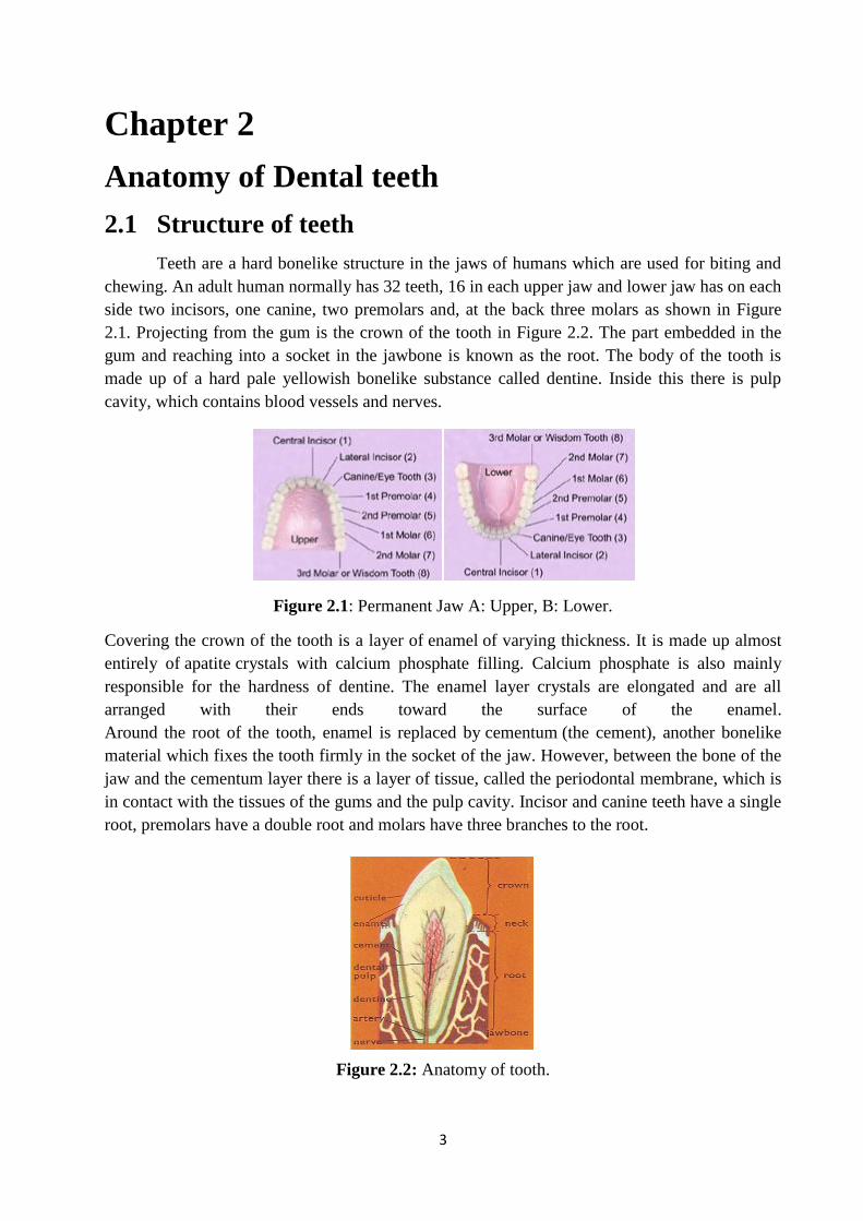
Figure 4.3: Epipolar geometry

The Figure 4.3 explains the epipolar geometry. The point „M‟ is imaged in two views at

the positions „X‟ and X‟. These points are in the image planes formed by the cameras with

camera matrices O and O´. As „M‟ varies, the set of all planes defined by the centres of the

cameras (O and O‟) and „M‟ forms a family of planes with baseline OO´ along ee´. The

correspondence between two points is defined by epipolar plane XOO´. The epipolar plane I´

will correspond to a point X, which is the intersection of epipolar plane and the other image

14

plane. This is symmetrically same for point X´. The expression for the back projected ray for the

first camera P form x and containing the center of first camera O is given as,

M ( ) = P+X + O (4.19)

where P+ is pseudo inverse of „P‟.

The epipolar line forming is

l´= (P´ O) x (P´P+ x)

The epipolar is P´O as shown in the Figure (4.3) and it is defined by the skew symmetric

matrix by the cross product. So the epipolar line in the second image of the point in the first

image is given by,

l´= [e´] x (P´ P

+ x) = F x (4.20)

Here,

F = [e´] x (Pl P

+) (4.21)

Where [e´]x skew symmetric matrix which introduces the rank 2 constraint on fundamental

matrix.

The relation between the 2D family of point and 1D family of lines is formed by a map induced

by F. So, finally

x´ (F x) = 0 (4.22)

This equation explains that x´ is required to prove the equation for an epipolar line of x

in the image I´. Equation (4.22) is nothing but epipolar constraint, which is satisfied by the

corresponding points in two images.

If [t]x represents the cross product corresponding to translation vector, then the coplanar

principle can be satisfied by

x´ ([t]x Rx) = 0, (4.23)

Where the essential matrix is

E = [t]x R. (4.24)

This expression will take the x´ to the image in the first plane. For uncalibrated case K

and K´ are used which are calibration matrices to transform the image points in pixels with point

in camera coordinate system. Comparing equations (4.23) and (4.24) will give,

(K-l x´)T

E (K-l x) = 0 (4.25)

15

Finally, the relation between essential and fundamental matrix is given as

F = K-T

EK-l

(4.26)

The intrinsic parameters and extrinsic parameters of the camera are both described by the

fundamental matrix, which is advantageous. This reveals that it only depends on matched points

in both the images. If there is a pure translation which is horizontal parallel, then there is no

change in internal parameters occurs and positions are differed by only translations.

It is given by

P=K [ Pl= K [I|-T] (4.27)

The equation (4.21) can be written as

F = [e´] x K K-l

(4.28)

(4.29)

The equation (4.29) is fundamental matrix for pure translation and in matrix form it becomes.

(4.30)

When we apply projective transform, the epipole is moved to a point at infinity horizontally this

process of estimation is called “projective rectification”.

After transformation the image points are given are given by,

= H x and (4.31)

The relation between , and F becomes

(4.32)

or

( ) = 0 (4.34)

Finally

F = H´ H (4.35)

The estimation of fundamental matrix F is needed to get the epipolar geometry. To find

F, initially we need point correspondences between images. If m´ is a point in the second image

with respect to the point m in the second image, then it must lie in epipolar line l´=FM and so

m´t. l´=0 [12, eq. 5.1]. Then the constraint on epipolar geometry is therefore,

m´t F m = 0 (4.36)

16

The equation (4.36) shows that F is estimated from 8 point matches in two images of

same scene. F has seven degrees of freedom as defined before. The constraint det (F) = 0 is

implied by rank 2 condition of 9 linear conditions modulo of matrix F (algebraically). So, F is

calculated by 7 matching points and a rank constraint and three possible solutions.

In [32] this procedure of automatic epipolar geometry algorithm is explained for good

out come and with some care. For 8 matched points (minimum), it may have noise. Then the

least squares approach gives good solution as:

(4.37)

The equation (4.37) calculates the eigen vector and this vector is for the smallest Eigen

value in symmetric positive semi definite normal matrix AtA. All these numerical techniques are

explained in [44]. The rank constraint is not imposed on it and so another computation needed to

be added to project the F on to rank 2 subspaces. This is done by SVD of F, SVD decomposes F

into

F=QDR (4.38)

where D is diagonal and Q, R is orthogonal. When D 0 the result is the desired one.

The method is unstable for application on images natively. Stability can be achieved

when the pixels are normalized from [0, 512] to [-1, 1] prior to calculation. This provides a

stable and accurate solution of F. But there is also a need of rejecting false correspondences in

the input data as in [16].

Summary:

The estimation epipolar geometry is:

1. Extract points from images

2. Find out point correspondences as in initial set

3. Estimate the fundamental matrix according to above algorithm

4. Least median square approach is used to estimate the results

5. And make it more robust.

17

4.2.1 RANdom Sampling Consensus (RANSAC)

RANSAC estimates the fundamental matrix form a set of point matches in two images of

same scene. The problem is that the matches obtained are not accurate. Point matches that satisfy

the estimated epipolar constraints are inliers and without are outliers. Outliers are resulted from

the inaccurate matching of points from the set of images. The estimation of error function

eliminates outliers by minimization process using threshold, which maximizes the number of

potential inliers.

4.2.2 RANSAC Algorithm for non-linear minimisation

The epipolar geometry of two images gives a set of matched points and the

correspondences between the images gives 8 point matches. The non-linear iterative version is

preferred for its robustness, and in combination with the RANSAC method, can be used to

eliminate potentially false matches. The idea is to randomly choose n samples from a set of N

point matches and find the corresponding fundamental matrix F by iterative minimization of a

distance function (4.39) or (4.40).

(4.39)

(4.40)

A threshold is applied to all of the N point matches to eliminate possible outliers using

error function. This process is repeated to get the best fundamental matrix with the most number

of inliers. Probability of selected set of point matches p of an outlier to all of n selected matches

as inliers is given by . The minimum samples to be tried for a set of selected point

matches consisting of inliers with probability P is given as,

(4.41)

An important factor in using RANSAC is to estimate the fundamental matrix with the

size of the sample set used in the iterations as in [5] [13] [3]. Once most of inliers are found, the

algorithm can be terminated. The difference between inliers and outliers are differentiated with

threshold epipolar distance as (4.42) and (4.43).

(4.42)

(4.43)

18

Computing F from (4.39) or (4.40) Using (4.43), determine the number of inliers

corresponding to this F in the N - set of points. If Z values for the fundamental matrix are

obtained, the set of fundamental matrices obtained, by choose the one that minimizes (4.39) or

(4.40) with the most number of inliers. An adaptation of this method of estimating the epipolar

geometry has been used to develop a rectification scheme that minimizes distortion in the

images.

4.3 Rectifying transforms for uncalibrated

To make the epipolar geometry simple, the steps we go through is a modified form of

epipolar constraint. As shown in (4.35). But to make the reconstruction look more close to real

image, it is required much that the constraints are imposed which relates to physical properties of

the image. The process starts directly with pre-computed matching points to rectify the pair of

images of same view. Disparate positions in space related by arbitrary rotation and translation

are constrained to lie on skewed lines in the image. These constraints on simplified geometry

after rectification process are still needed to resemble the rectified images as original images.

The epipolar constraint is given as

X ´T F X = 0 (4.44)

and then

X T F

T X ´= 0 (4.45)

This constraint reduces epipolar geometry to a canonical form and represents pure translation.

The fundamental matrix for rectifying transforms are given as

F = H ´T H (4.46)

The transformations which satisfy (4.46) are not unique and so exact choice of the transform is

not made. This may lead noticeable distortion in the rectified images.

4.3.1 Approach to uncalibrated rectification

The uncalibrated rectification is done in three folds. First, a parameterization of the

transforms, second factorisation of fundamental matrix and followed by defining a cost function

to estimate epipolar geometry for a detailed geometric condition and third constraints on the

transforms at the same time to reduce visual distortion.

The factorisation and parameterisation is explained simultaneously, below as in [15] the

transformation „H‟ in projective method can be represented as product of two matrices,

H = (H-l)-l

= (QhRh)-l

= RHQH (4.47)

This is true as Q is an upper triangular matrix and R is an orthogonal rotational matrix.

19

R is represented about x-, y- and z- axis and so R=Rx Ry Rz and Rz is orthogonal matrix so finally

the homography matrix is represented as [17],

(4.48)

Replace in (4.48) with RH for first matrix, QH for second matrix, Ry is third matrix and RX for

fourth matrix.

This look like segmenting the homography matrix which is same as

H = Hs Ha Hp (4.49)

Here s - similarity, a - affine and p - projective component of H.

Finally the H is described with parameters as

(4.50)

Where „ ‟ is rotation in image plane. It can be chosen to make the second coordinate of the

epipole to zero for epipolar lines parallel to x-axis. Scaling and skewing are represented by QH.

Projective rectification for unrectified images by (4.44) will give fundamental matrix

with independent of first rows. This is due to criteria of and so the estimation results from (2)

as, [5]

(4.51)

When we attribute only of the tilting and panning to one of image and the later to other

image of the same seen, there is chance in reduction of degrees of freedom and so, the (4.49)

reduces to

(4.51)

Finally can be used to build , which is given by (4.51)

(4.52)

4.3.2 Transformation constraints

Considering which describes the fundamental matrices in terms of rectifying

homographies reveal that constraints on the fundamental matrix estimation are also applied to

estimate the rectifying transforms. Also, there are conditions to be considered to find the

rectifying homographies minimized with constraints justified has physical significance. Firstly,

the geometric distortion is reduced by using (4.42) and (4.43) extended to include epipolar lines

to get symmetric distance criterion as [16] in terms of (6.10)

(4.53)

20

whenever there is uncertainty of matched points, the total cost (4.53) is inversely proportional to

its variance [16]. Finally minimization over F to minimize the cost as, [16]

(4.54)

Second one is visual distortion reduction by orthogonality and aspect ratio. The

constraints also should consider the inclusion of orthogonality and relative sizes of the image by

looking over it as in [17][18].

The orthogonality in the image is the perpendicular condition between the epipolar line

and to pixel columns. To reduce this, error pixel information of the rectified image is used as in

[17] and also aspect ratios are used to obtain inimitable cost function. The minimization problem

for the estimation of rectifying transformations are given as in [5]

(4.55)

Here

(4.56)

By ortohgonality principle of

Also, x, y and xH, yH are axis defined as the difference vectors in the affine image plane of

original and rectified images respectively.

4.3.3 Affine correction:

The estimation of transformations is more related to projectivities and there is a chance

for skewing error for horizontally non uniform scaling. Therefore orthogonality and aspect ratio

is re written with Ha included. As [9],

(Ha xH) T

(Ha yH) = 0 (4.57)

and

(4.58)

where Ha is parameterized affine transformation given by,

(4.59)

And

as in [5]

21

4.4 Methodologies for X-ray Calibration

To estimate the parameter for transforming a 3D space point to a 2D image point via a

camera, the important requirement is to calibrate the camera. Once it is done we can transform

between world and image plane.

4.4.1 Camera imaging

The Figure 4.4 explains the analogy between x ray imaging system and camera imaging

system. The only difference is relative position of object, image plane and lens or image

intensifier.

Figure 4.4: Camera imaging system and x-ray imaging system

4.4.2 Existing calibration methodologies of x ray source

X-ray calibration setup designed for NDT applications which is already existed is

considered. The setup is a cone beam x-ray radiography system which has an x-ray source

manipulator of the inspected specimen and x-ray detector. The system setup is analogous to our

system but only the inspected specimen is replaced by patient and the detector used here is for

NDT applications which have 200-400 Kev X-ray. The detector in medical applications is

replaced with 20-180 ev image intensifiers. The schematic of the setup is shown in Figure (4.4).

In this method the X-rays are detected by the image intensifier which is amplified and depicted

on a phosphor screen image intensifier which converts the x-rays projection to a visible

radioscopic image.

22

4.4.3 Geometric model

The object coordinate system is similar to the one explained to the system in previous

chapters. The notation is used as in [28] to differentiate between the projective geometry. In this

method the origin O is the centre of rotation of the object.

There are two methods for x ray calibration of which reviewed first is the calibration of

tomography and radiography systems and second is about calibration of 3D vision system. The

tomography system calibrations will classify its geometric properties into two parts as intrinsic

and extrinsic. In general the intrinsic parameters are constant and related to x-ray detection

system geometry. For the later, there is a need of regular estimation as it relates to variations of

the object under inspection. Alignment and nonlinear minimisation of projection matrices are

used as [19] [20]. High precision, fast estimation and special calibration object are requirements

in these methods. The camera calibration methods follow a two stage approach by geometric

constraints. Precision is good for a compromise on speed of measurement. This is shown in

[23].In [9] estimation by nonlinear minimization for only the extrinsic parameters and usage of

[22] method to state with good initial estimate and fast convergence to solution is applied.

The geometry of the radiography system is shown in the Figure 4.5 which includes all

geometric configurations explained. It has source, detector and object.

Figure 4.5: Radiography system geometry

The point M on the object is (x, y, z) in Figure 4.5. M is related to x-ray coordinate system by

(4.61)

where , , are coordinates of F in object coordinates . Also the three successive rotations

of the object coordinate systems are R (δ), R(ξ) and R(ψ).

R= R (δ), R (ξ), R (ψ) (4.62)

23

4.4.4 Estimation of intrinsic and extrinsic parameters.

The parameters ( ) are intrinsic parameters. P and q are calculated by the

detector screen plane in radiography system and as in [21] where image plane and detector plane

is not same [tomography systems]. The extrinsic parameters are calculated by nonlinear

minimization method where cost function is

(4.63)

where i is a point in N calibration points.

Pixels coordinates are given by

(4.64)

(4.65)

In [5], a detailed explanation and its performance with simulations are presented. The

minimization is started with a initial guess by vanishing lines methods as in [4] as shown in

figure. It uses the grid of sphere whose lines of joining are not parallel in image plane by

vanishing line perspective geometry.

Figure 4.6: Vanishing points and Vanishing line of a Hexagonal calibration object [9]

Figure 4.7: Initial position of the calibration grid for vanishing lines method [9]

24

Means of vanishing point of all grid points which are center of spheres of the calibration

object are calculated. The vanishing lines are calculated by least square method with respect to

detector coordinates system „Gd‟, the method uses Euler given by . So, it becomes

analogous as world to camera coordinates transformation with object to x ray source coordinate

system described by (1)

4.5 Self Calibration of Biplane X-ray imaging system:

To show a good visualisation of structure of interest in mouth of a patient, the direction

of camera is specified by two angles as right-left and angulations [30]. The right – left

angulations are chosen by the clinician according to the morphology of total jaw. The different

coordinate system is considered as shown in the Figure 4.7.

Figure 4.8: Geometry of Biplane X-ray Imaging system

The positions of the X-ray system at S1, S2 and R1 = (S1, x1, y1, z1), R2 = (S2, x2, y2, z2) are

the positions of the two X-ray system. The linear transformations are applied for simplicity to

model the perspective view of 3D object point on left and right image.

Now the system calibration matrices are calculated as in [30].

= Mi

for i = 1, 2 (4.67)

where w is a scaling factor ; u, v are image coordinates and (X, Y, Z) is the 3D point.

Explicit representation geometrically,

Mi = P (di , sp, usi, vsi ) Di for i = 1,2 (4.68)

25

If Di is the displacement from object to source, sp known pixel size, linear transformation

in homogenous coordinates of perspective image of 3D point and R, Ri are object and source

coordinates respectively. Now the matrix representation is given as [39],

=

(4.69)

If the movement of cone-beam is adjusted by the doctor, then angulations are α along x-

axis, β rotation along y-axis and translation along z-axis which are measurable here. Then

finally is given by,

= ( ) (4.70)

Equation (4.68) and (4.70) will give,

(4.71)

The mean square error of the system between the analytical coordinates in the object and

the matched points calculated by the doctor from two images of same teeth is minimized. The

matched points are found by RANSAC algorithm. The Mathematical expression is given by

[30],

The equation (4.72) d [ ] gives Euclidean distance. Also, u,v are projection coordinates

obtained from (4.67) and (4.71); n is nth

reference point of Pn; i is ith

plane. The iterations are

continued with correction of at every time and this will continue until a predefined

minimum error is achieved. The total 3D reconstruction process is clearly framed in [30] which

include robust estimation and accuracy even in presence of noise.

Summary: In this Chapter the calibration methodologies of x-ray source is introduced. Also,

self calibration of the X-ray imaging system is explained. This methodology reveals the fact of

its complexity and uses linear transformation for simplicity. In chapter (6) in contrast to these

methodologies, a novel simple and popular methodology is explained which re-renders bi-plane

images and transformation or X-ray recovery matrix (XRM) is found to calculate 3D

information like angle position of centre of images for 3D reconstruction.

26

Chapter 5

Simulation of X-ray Radiographs from optical images

5.1 Introduction of X-ray radiography The real image is the one which is real, physical and it may be photography or a

radiograph of X-ray. These images are helpful for scientific measurement.

X-ray when targeted to a sensitive material like fluorescent material will emit light which are of

varying light intensities. These are similar to television screen. The schematic of this method is

shown in this Figure (5.1).

Emission of intensity

high for high intensity

incident radiation

X-ray

Low emitted light

intensity.

Florescent layer

Figure 5.1: Effect of intensity on florescent screen

The fluorescent layer doesn‟t need any light source to see. We can see it using naked eye.

5.2 Image Characteristics The image formed by fluorescent screen has following characteristics.

1. Noise

2. Contrast

3. Sharpness

4. Resolution

5.2.1 Contrast

In order to identify the structure in a radiograph it must be of different optical density

when compared to adjacent ones. Contrast is feature of the images which is the variation of

intensity distribution of energy, phase, relaxation characteristics etc, the total outline is the

contrast is the nothing but finding the variations in density or luminance if the differences are

great we can say the contrast is high and so the vice versa.

27

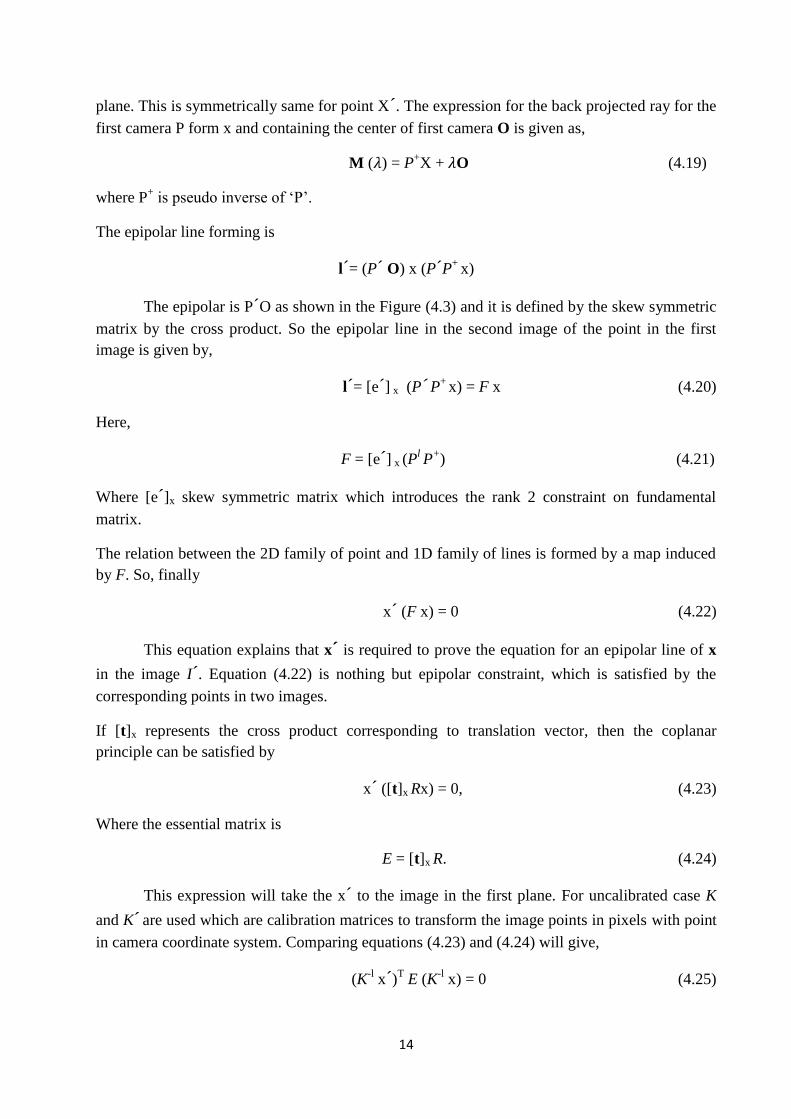
To explain this contrast mathematically, let us take an example of situation of projection

radiography. The area is exposed to uniform beam of x rays photons of (no). The area exposed is

a slab of tissue with linear attenuation coefficient „u‟ and thickness x.

There is also variation towards the right which is small increases of „Z‟. The illustration is

shown dogmatically in the figure (5.2).

Figure 5.2: X-ray imaging Ref. [10]

The increased thickness areas and remaining is exited by x ray fluency (photon/m2) of amount

„B‟ and „A‟ respectively. Now the contrast is measured as

Now with the thickness

„x‟ we have attenuation which is equal to for

(5.1)

(5.2)

So, C (5.3)

which explains that the variation in the surface cause contrast and increases overall contrast.

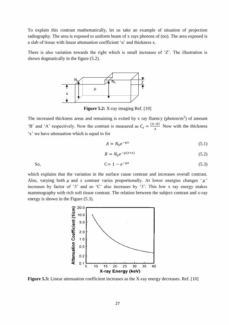
Also, varying both and z contrast varies proportionally. At lower energies changes „ ‟

increases by factor of „3‟ and so „C‟ also increases by „3‟. This low x ray energy makes

mammography with rich soft tissue contrast. The relation between the subject contrast and x-ray

energy is shown in the Figure (5.3).

Figure 5.3: Linear attenuation coefficient increases as the X-ray energy decreases. Ref. [10]

Z

x

No No

28

5.2.2 Detector contrast:

For small variation in the input energy there will be considerable big changes in signal or

contrast of image. So the detectors characteristics play an important role in producing the final

contrast. A graph between the detected energy and output signal will till about detector contrast

„Cd‟. The curve explains the characteristics of it there are mainly two of them which are linear

and logarithmic this shown in Figure (5.4).

Figure 5.4: Characteristic curve A: logarithmic response in radiographs. B: linear in flat

imaging system. Ref. [10]

Most of the systems have linear characteristics; the slope(r) measurement of the curve will

explain about the characteristics and is given as.

(5.4)

Here A and B are adjacent regions. For radiographic contrast is given by RC=ODA-ODB, since

the analog film is the output.

5.2.3 Contrast to noise ratio (CNR)

The CNR is a meaning full and frequently used measurement to justify the quality of the

image. For digital image acquired by detector systems, a common processing technique is

subtraction of a constant number „K‟.

Suppose let us take there are two regions which have average values of A and B. So, after

processing it is

(A-K)(B-K) (5.5)

As per the equation (5.5),

(5.6)

29

And as K=A it will be undefined. So a meaningful measurement is,

(5.7)

Where is the noise in the image. This helps to do post process and noise measurement will

give relevant CNR. For digital images, a gray scale plot is drawn, which is histogram of the

image as shown in figure (5.4). A and B curves are used to produce two images. The slope of the

look up table is related to displayed image contrast.

5.3 Spatial resolution and point spread function (PSF)

In general spatial resolution is the measurement of the quality of the system to distinguish

two objects as they become closer and smaller. The ability of the system can be measured from

the 3-dimentional parameters of a 2-dimentional image. They are height, width and greyscale.

So, there measurement tells how accurately the system can depict objects in two spatial

dimensions. Those two are width (x-axis) and length(y-dimension).

One way of measuring this spatial resolution is to stimulate the detectors system with a

single point input and look over its response. The stimulation by single point source to a detector

system gives a point spread function. The diagrammatic representation of this is shown in Figure

(5.5)

Figure 5.5: Blurring due to an imaging system

The PSF is used for image restoration problem. Since, the image individual pixels

exposed to PSF will blur it individually this is similar to a mathematical method called

convolution and given as.

(5.7)

Where is image and is the object, „h‟ is PSF which has input and output

parameters separated by “;” h(x, y) is additive noise function.

There for image restoration the factors required are

1. PSF

2. Blurred image

3. Finding the statically properties of noise

Imaging System

Input Output

Noise

30

Blurring in images depends on many factors like defocusing, propagation of light

photons. By optical diffusion horizontally and laterally due to thicker screens and motion

blurring in all imaging modalities PSF introduces more blurring, if it is non isotropic for various

physical reasons.

5.3.1 Line and edge spread functions

The inability to stimulate the system with a very small 0.010mm diameter will make use

of line spread function (LSF) and edge spread function (ESF). Also when stationary imaging

system with a isotropic as show in Figure 5.6A, LSF is enough to describe the behaviour for a

situation as shown in Figure 5.6B where PSF is non isotropic, LSF measurement with line

impulse at different angles is required for understanding the image system. Finally, ESF is

calculated when we need to learn spatial properties of x-rays scattering.

Figure 5.6: A: Isometric display of point stimulus B: PSF rotationally symmetric.

5.3.2 Frequency Domain of PSF

PSF is not constant over the entire field of view in many optical systems, optical

aberrations vary with field angle. A region of the image with approximately constant blur is

sometimes called an isoplanatic patch, optical systems are linear and shift-invariant over

isoplanatic region of the field of view.

Figure 5.7: Clock being imaged by a lens onto a screen; a point source in the scene (upper

Right) becomes a point-spread-function blur in the image (lower left).Ref [14]

The image within an isoplanatic patch can be represented as a convolution of the PSF

over the scene. If h(x, y) represents the spatial shape (the intensity distribution) of the PSF,

(A) Point Stimulus (B) Isotropic PSF

31

then h(x – x', y – y') represents a PSF at location (x', y') in the image plane. Let

describe the brightness of the scene, and describe the brightness of the image [14].

(5.8)

Each point in the scene radiates independently and produces a point PSF in the image

plane with corresponding intensity and position. The image is a linear superposition of the

resulting PSFs. Mathematically, that result is obtained by convolving the optical PSF over

the scene intensity distribution to produce the image. Since a convolution in space

corresponds to a multiplication in frequency, the optical system is a spatial filter.

(5.9)

Where = Fourier transform of image, = Fourier transform of scene and

= the optical transform function (OTF). and are spatial frequencies in the x and y

direction, respectively. The units of and are cycles per mill radian (mrad-1

). The OTF is the

Fourier transform of the PSF h(x, y). However, in order to keep the image intensity proportional

to scene intensity, the OTF of the optics is normalized by the total area under the PSF blur spot.

(5.10)

The MTF of the optics is the magnitude of the function . Any blurring of the

mage can be treated as an MTF as long as the blur is constant over the entire image.

5.3.3 Spatial and frequency domain filtering

In space, the output of an LSI system is the input convolved with the system impulse

response. As shown in Figure 5.8. The system is a simple lens imaging the transparency of a

four-bar target. Given that the lens blur is the same across the field of view, the system is LSI.

The output image is the transparency intensity convolved with the lens PSF.

Figure 5.8: Spatial filtering in an optical system. Ref. [14]

In frequency domain filtering the two-dimensional Fourier transform of the scene

intensity is taken. The input spectrum clearly shows the fundamental harmonic of the four-bar

target in the horizontal direction. The higher-order harmonics are difficult to see because they

have less amplitude than have the fundamental harmonics. The Fourier transform of the

32

image is obtained by multiplying the Fourier transform of the scene by the Fourier

transform of the PSF. The output image is found by taking the inverse transform of the product.

The resulting image is identical to that given by the spatial convolution of the PSF in the

space domain. In Fig. 5.9, the direct-current component of the input transfers, and output

frequency spectrums has been removed so that the higher-frequency components are visible.

Otherwise, all that would be seen is a bright point in the middle of the picture. LSI imaging

system analysis can be performed using two methods: spatial domain analysis and

frequency domain analysis. The results given by these analyses are identical, although

frequency domain analysis has an advantage. Equations (5.8) and (5.10) both involve double

integrals. However, an image has many components MTFs. Using Equation (5.8) involves

calculating double integrals for line-of-sight, diffraction, optical aberration, detector, digital

filtering, display and eyeball.

Figure 5.9: Frequency domain filtering in an optical system. Ref [14]

Using Equation (5.10) involves double integrals to find the Fourier transform of the

scene and a second double integral to find the spatial image. Intervening calculations involve

multiplying the various component MTFs. Fourier domain analysis is used because it provides

accurate results with reduced computation.

33

Chapter 6

Experimental results

6.1 Data Sets

Radiographs Description

Per apical Obtained from a patient in a clinic in India. This is a 6 Incisor teeth

radiograph of the upper jaw.

Bitewing

Obtained from Radiology Dept. Karolinska Hospital, Stockholm.

The jaw images of a real skull are taken and the experimental setup

in the Lab is shown in the Figure 6.1. The algorithm is tested on 3

molar teeth images of the upper and lower jaw. Fig 6.3

Simulated To validate the result the optical images taken from the digital

camera of a lower jaw phantom is simulated as an X-ray image with

help of suitable filter as explained in section 6.4.

Table 6.1: Data sets used for Experiment

6.2 System Model overview

The model of the system is clearly explained in the Figure 6.1. In the next sections we introduce

our algorithm and its validation process. Before that the overview of it is explained in the form

of block diagram.

Figure 6.1: System Model

34

The data flow diagram of the algorithm proposed in this project is shown in Figure 6.2.

The process explained in this flow diagram is repeated for all data sets to obtain its 3D positions.

Finally visual validation is done to validate the methodology proposed in this project.

Figure 6.2: Flow chart of the system model

Start

Images Data set

Select Matched Points From image pair

Rendering of images

Obtain X-ray recovery matrices (XRM)

Transform XRM to Euclidian coordinate’s plane

Find the centre of the image

Plot the centers of

X-ray images in

the 3D plane

Stop

Images count check

No of Image

35

6.3 Obtaining matched features

The designed algorithm was applied to all uncalibrated stereo pairs for Periapical x-ray

radiographs, Bite wing x-rays and simulated x-ray radiographs from optical images taken from

Sony W110 Digital camera with resolution 1 mega pixel. The distortion of the radiograph

images of the Periapical and Bitewing x-rays are selected to be minimum and maximum overlap

to get better results for this experiment. The computation of matched points can be done

automatically as in [5], but the points are selected manually to minimize the error. As it is

obvious that the x-ray images are highly distorted, the selection is manual instead of automized.

RANSAC algorithm is used to discard the Outliers of the stereo pair images. As mentioned in

[5] the RANSAC method is tested for different set of images.

6.4 Implementation of Algorithm

Further to the discussion of self rectification in section 4.7 the methodology and

modifications of the algorithm are introduced in this section which follows experimental results.

In our work the estimation of fundamental matrix is constructed from the transformation matrix

pair according to limitation geometry which is done by iterative weight distance minimisation.

The weight distance is function included with a point and corresponding epipolar line. After that

the biplane images are re-rendered such that pair of points of same scene has minimum vertical

disparity in a horizontal minimum and minimum intensity variation.

Figure 6.3.1: Setup to take X-ray.

The experimental setups to capture the Bitewing and Periapical X-ray images are shown

in Figure 6.3.1. The detector is placed inside the mouth with help of T-stand and imaging

process is done as explained in chapter 3. In our project we have taken the real skull which is

supported by Oral Radiology department of Karolinska hospital, Stockholm. Two Periapical X-

ray images of Incisor upper teeth as shown in Figure 6.3 are used for the experiment. The

observation of two images will make known that 4 teeth are similar in both the images and

which is enough to apply the proposed algorithm and find the matched points. The same

observations can be observed in any pair of adjacent radiographs. This is the supporting point to

start the process of applying stereoscopic technique for all Dental X-rays.

36

The visual inspection of the two images in Figure 6.3 will clearly show the difficulty of selecting

the matched points of same intensity. So, the images are transformed to new positions by

applying the algorithm to make it parallel such that varying distance from the X-ray source is

minimised.

Figure 6.3: Periapical X-ray Radiographs of Incisor upper teeth.

The X-ray replacement process flows first with the Fundamental matrix estimation derived from

transformation with maximum inliers and minimum error and then it ends with selecting the

matched points manually and reducing the vertical disparity of pair of images to render images.

The Figure 6.4 shows the output of the program (developed in MATLAB) after selecting the

matched points and epipolar lines of the respective points in the adjacent pair of radiographs.

The algorithm rectifies the images and makes the selected matched points to be accurate.

Figure 6.4: Computed Epipolar Geometry

If ( , ) are points which are selected by the doctor manually in the two images of same

teeth and X-ray recovery matrices XR and XR are pair of estimated transform used to describe

the fundamental matrix F. The mathematically it is given as,

37

This equation represents the optimal estimate of F which used minimum error of (A, A ). After the implementation of the algorithm the results of the experiment is shown in the Figure

6.5. The points are selected manually in order to introduce minimal error, since the radiographs

as seen are highly distorted, less resolution and more disparity in intensity.

Figure 6.5: 3D position recovered images using uncalibrated algorithm

XRM‟s are calculated by the program after the recovery process, which has translation and

rotation information for transforming from image plane to projective plane. The XR matrices of

the two radiographs are used in the next sections for placing the images in the 3D plane. The

Procedure to find 3D Points

1. Frame corners points P (2x4) in Euclidian coordinate system are computed from the given

image.

2. Image frame corners in Euclidian coordinates P (2x4) are transformed into Homogenise

coordinate PH (3x4).

3. Obtained transformation matrices (XRM) of the image PXR (3x3) from our algorithm is

multiplied with the Homogenise coordinate PH (3x4).

4. Homogenise image frame H(3x4) from the step 3 is normalised and transformed to

Euclidian coordinate plane E(2x4), contains the four corners of the image.

5. Using the obtained image frame in Euclidian coordinate space the centre of the image is

calculated with the un-transformed image frame, and it is plotted in the 3D coordinate

system.

6. Similarly the process is repeated for all images in a particular data set.

38

From the obtained XRM‟s the 3D positions of the teeth from the 2D radiographs is found by

the program designed as per the above procedure. Plot of the centres in the 3D plane is shown in

the Figure 6.6.

Figure 6.6: 3D Points for two x-ray images

The process of taking the x-ray radiographs for full teeth around the structure as shown in the

Figure 6.7. The novelty of our methodology is solving the problem of re-rendering randomly

capture of the radiographs for finding its 3D positions. As mentioned the source is moved

randomly by clinician around the mouth in order to get the good projection of the image and also

in order to cover the tooth till the root especially in Periapical X-rays.

Figure 6.7: Process taking X-ray radiograph to teeth

C

1

2

39

The set of radiographs for full mouth of Periapical X-rays are obtained as per the

procedure explained above which is shown in Figure 6.8

Figure 6.8: Dental X-ray images of the teeth

The adjacent pairs are selected manually and applied to our procedure explained above.

Finally the process is repeated for all the pairs, XRM‟s are obtained and the points are plotted,

the result of total process indicates 3d positions of teeth as shown in the below Figure 6.9. The

radiographs are transformed by our algorithm such that the distance variation from the X-ray

source and also the intensity distortion of the same scene in the adjacent radiographs are

minimized. Finally, the total set radiographs are placed in 3D space to find relative position

between them as in Figure 6.6.

Figure 6.9: 3D Positions of Centre of Radiographs of teeth

40

6.5 Visual Evaluation for Bitewing Radiographs

In Intra Oral radiology the two major methods are Bitewing and Intra Oral radiography. As

per the requirement clinician use one of the methods for diagnosis. In this radiographs the

detector is placed on the T stand as shown in experimental setup. The clinician adjusts the X-ray

source by the special arrangement so that the rays are perpendicular to detector and also the

image also projective. This gives the exact image of the teeth in terms of size and area. The

adjacent pair of images is applied to our algorithm, its epipolar lines, XRM‟s are found and its

center is plotted in 3D space. The total process is shown in the Figures 6.11 to 6.15.

Figure 6.11: Bitewing X-ray radiograph

Figure 6.12: Computed Epipolar Geometry

Figure 6.13: 3D position recovered Bitewing Radiograph

First rectified image Second rectified image

41

Figure 6.14: Full mouth set of Bitewing X-rays

Figure 6.15: 3D Positions of Centres of Bitewing X-rays.

6.6 Validation of the results

To validate our results the images are taken with known position information as the x-ray

image will not have any information regarding the position of the teeth. A model of the teeth is

taken to know the information of the position at which the image is taken and then obtained

images are applied to our algorithm in order to validate the results. The algorithm is also applied

for the square box to validate and then applied for the dental teeth model which is prepared with

real set of teeth and cement material, as shown in Figure 6.16.

42

Figure 6.16: Models of dental lower teeth A: Real Teeth fixed in the model, B: teeth

model made with Gypsum product.

The images are taken with a fixed angle and distance with a digital camera around the

teeth model. Later the model is rotated for other angles with help of a scale and the camera at

fixed in position. The arrangement setup is shown in Figure 6.17.

Figure 6.17: Experimental Setup to take optical images

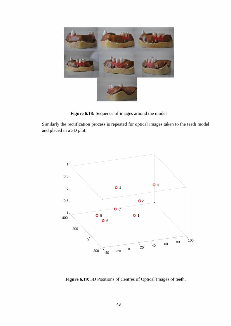
43

Figure 6.18: Sequence of images around the model

Similarly the rectification process is repeated for optical images taken to the teeth model

and placed in a 3D plot.

Figure 6.19: 3D Positions of Centres of Optical Images of teeth.

-40 -200 20

40 6080 100

-200

0

200

400

-1

-0.5

0

0.5

1

C

1

3

2

4

5

6

44

6.7 Validation of angle between each image using

transformation (XRM) matrix.

The XRM‟s between several images are calculated from different data sets where only

one camera is used for teeth models and square box (Fig 6.16). The variation of angle is 45

degrees. The change in camera angle between each image is estimated from the projective

components namely rotation in image plane, panning and tilting in XRM as in equation (6.5).

The values in the results in the XR matrix calculated from our algorithm are in radians and so,

we converted it to degree and tabulated in Table 6.1. The variation of angle calculated and the

known angle are around (0-100) which validates our methodology and can be used for any type

of images.

Pair of images

Square Box Actual Angle (450)

Difference in angle(0)

Teeth Model real teeth Actual Angle (300)

Difference in angle(0)

Teeth Model ceramic lower Actual Angle (300)

Difference in angle(0)

Teeth Model ceramic upper Actual Angle (300)

Difference in angle(0)

1-2 48.79 3.79 35.80 5.80 30.26 0.26 28.52 -1.48

2-3 44.02 -0.98 33.99 3.99 38.12 8.12 40.06 10.06

3-4 46.69 1.69 40.23 10.23 39.27 9.27 29.30 -0.70

4-5 51.56 6.56 33.43 3.43 25.61 -4.39 22.83 -7.17

5-6 41.69 -3.31 26.68 -3.32 41.02 11.02 36.45 6.45

6-7 50.53 5.53 40.68 10.68 36.81 6.81 37.74 7.74

7-8 46.10 1.10 25.33 -4.67 33.49 3.49

8-9 43.82 -1.18

9-10 48.79 3.79

10-11 44.02 -0.98

Average error

3.24 5.98 5.48 6.63

Table 6.2 Angle measurements between individual optical images

The angles of the radiographs taken from single X-ray source are calculated and

tabulated in 6.3 for Periapical and Bite wing radiographs.

Pair of images

X-ray(lower Periapical)

X-ray (Teeth lower) X-ray( teeth upper)

X-rays(Bite-wing)

1-2 59.91 49.07 62.21 44.95

2-3 52.49 42.26 44.08 36.97

3-4 55.19 35.95 48.47

4-5 52.11 51.73 No match

5-6 44.25 51.07 59.99

6-7 47.05

7-8 36.68

Table 6.3 Angle measurements between individual Radiographs

45

6.8 Validating with simulated X-Ray Radiograph

To validate the 3D positions obtained from original 2D X-ray images the simulation of the

X-ray images is need to obtain with known information. In this section the process of simulation

is explained. The method we used SRS 78 Spectrum processor to generate the PSF of scatter and

blurring response. By considering the X-ray system source parameters with tube target material

as tungsten, tube voltage source as 70KVp and anode angle 15 degrees, the material to be

attenuated for both bone and tissue is considered with 5mm thickness. The processer simulates

the spectrum and photon attenuation is obtained for both the materials. To approximate the PSF

of the x-ray system, Gaussian function is used which is multiplied with the photon attenuation

spectrum referred as MTF [34]. Then it is been multiplied with the Fast Fourier transform of the

bone and tissue segmented binary optical image. Finally Inverse Fourier transform is applied to

obtain the simulated X-ray Radiograph. The flow chat is show below in Figure 6.20.

Figure 6.20 Flow Diagram of X-ray Simulation.

6.9 X-ray transfer function for bone and Tissue

Two-dimensional point spread function (2D-PSF) The simulation of X-ray image „ I ‟

can modelled as blurred version of x-ray image „ i „, from the equation (6.2) shown below

(6.2)

Where is the blurring function, the true image I can be solved if kernel h is

obtained. The effect of scattering and collimator blurring in the 2D image domain is normally

hard to obtain. The 2D-PSF is spatially variant which changes for every pixel in the image;

effective scatter in source image is different when a projection is applied. The estimated

46

020

4060

80100

0

50

1000

0.2

0.4

0.6

0.8

1

scattered projection for any projected blurring kernel is obtained by the SRS 78 spectrum

processor by giving the parameters like anode voltage and the angle at which beam is focussed

to the tungsten and the thickness of the material to be attenuated [33]. The amplitude of the 2D-

PSF is determined from the obtained spectrum of the mean average voltage. The shape of the

PSF is determined as in [32]. In which it is observed that the Gaussian function fits the overall

shape of the blurring function for 2D-PSF. The magnitude of Gaussian A0 is taken from the

mean average voltage from the spectrum. The full width half maximum in the long-axis and

short-axis direction as FWHMl and FWHMs, and the center (x0, y0),

(6.3)

Where , and FWHMs are the functions of the point source position (x0, y0). 2D-PSF

and its corresponding Gaussian function are shown in the Figure 6.22, for Bone and Tissue the

Gaussian function with parameters fitted to the 2D-PSF. And corresponding magnitude of PSF

are shown in the Figure 6.23. The segmented radiograph is shown in the Figure 6.21 for bone

and tissue.

Figure 6.21: Segmented image of the teeth for bone and tissue.

Figure 6.22: Bone and Tissue 2D-PSF.

010

2030

4050

6070

8090

100

010

2030

4050

6070

8090

100

0

0.1

0.2

0.3

0.4

0.5

0.6

0.7

0.8

0.9

1

47

Figure 6.23: Magnitude of 2D-PSF for bone and tissue.

The segmented images shown in the Figure 6.21 are Fourier transformed and multiplied with the

respective 2D-PSF for bone and tissue, later both the images are added and inverse Fourier

transform in applied to obtain the simulated x-ray scattered image for the give segmented

images, the result for proposed simulated method is shown in the Figure 6.24

Figure 6.24 Simulated X-ray radiograph.

Pair of simulated X-ray radiograph in the Figure 6.25, is applied to the proposed algorithm and

its results are shown Figure 6.26-27.

Figure 6.25: Pair of simulated x-rays

simulated x ray

100 200 300 400 500 600

100

200

300

400

500

600

simulated x ray

100 200 300 400 500 600

100

200

300

400

500

600

simulated x ray

100 200 300 400 500 600

100

200

300

400

500

600

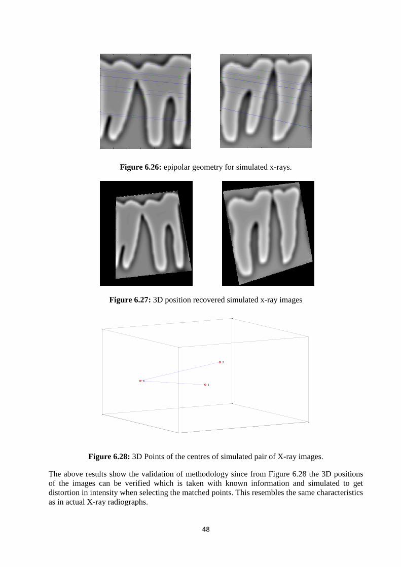
48

Figure 6.26: epipolar geometry for simulated x-rays.

Figure 6.27: 3D position recovered simulated x-ray images

Figure 6.28: 3D Points of the centres of simulated pair of X-ray images.

The above results show the validation of methodology since from Figure 6.28 the 3D positions

of the images can be verified which is taken with known information and simulated to get

distortion in intensity when selecting the matched points. This resembles the same characteristics

as in actual X-ray radiographs.

First rectified image Second rectified image

C

1

2

49

Chapter 7

Conclusion

In this thesis work the relative position of x-ray radiographs in 3D plane are calculated

by re-rendering two radiographs of the same scene using two transformation matrices (XRM).

The calculated matrices replace the 3D position of images to an optimal position where the

intensity distortion due to varying distance from the x-ray sources in the two radiographs are

minimized. The angle information between adjacent pair radiographs from different data sets are

also calculated by using the XRM matrices and are presented in Table 6.2 and Table 6.3. The

dataset consists of optical images of the real teeth model, square box and ceramic teeth model

with known 3D information. The result shows an average error of 3.240 and 5.98

0 in comparison

of estimated to actual values for square box and teeth model respectively. Visual inspection was

also achieved by presenting the centre of image planes which verified the placement of the

images. We used also a set of radiographs provided by Karolinska Hospital, Stockholm, Sweden.

The result of direction angle of this data set is presented in table 6.3 and is also demonstrated in

figure 6.15.

Due to strengthen our validation, pre information of radiographs positions were needed.

However to obtain enough datasets was difficult due to confidentiality of patient information.

Therefore we proposed a new methodology to simulate X-ray images from optical ones which

concluded as a jewel to crown of this work. The simulation of radiographs is done in two folds.

The detector is modelled by calculating the Modular Transfer Function of bone and tissue, using

Spectrum processor [33] based on photon emission principle. The product of Fourier transform

of the image and MTF is calculated and the virtual radiograph is obtained by its Inverse Fourier.

The 3D positions of simulated radiographs are presented in figure 6.28 which verifies the

methodology.

The two novel methods, 3D positioning and simulation of X-ray images, can be

implemented in further applications. Having position of two radiographs it is possible to render

an intermediate radiograph image based on different methods, e.g. image-based rendering. These

images can be used to present the 3D information in 3D displays. The 3D structure can also be

reconstructed as far as we have less distortion in the X-ray images due to the distance problem.

In conjunction to the oral radiology education, the simulator can be used to clarify the

functionality of existing system by possible variation of the involved parameters.

50

Chapter 8

Acknowledgement

This thesis is finally finished and our work at BTH is done. It was a great time and much fun to

work in computer vision and image processing, with this foundation venkata prasad dandey got

PhD in ETH, Switzerland. So we thank all the people who made it possible.

We would like to express greatest respect and gratitude to Siamak Khatibi, our supervisor at

BTH, for supporting us during this thesis, helping us with his greatest knowledge about

computer vision and Image processing and many great hours in guiding us to finish work.

Karin Nasström ( Chief, Department of Oral Radiology, Karolinska Hospital, Stockholm) for

giving great support in providing X-ray system, to take radiographs with help of her assistant.

Bitra Srikanth (BDS), with whom we got motivation to proceed our thesis by providing the

models of the dental teeth jaw.

Our parents and fellow students for supporting us.

51

Bibliography

[1] Mark Nixon, Alberto Aguado, Feature Extraction & Image Processing, Newnes, Oxford,

2002, pp. 16l–214.

[2] D. H. Ballard and C. M. Brown. Computer Vision. Prentice Hall, New Jersey 1982.

[3] Lalit I. Abhishek V. Robust Uncalibrated Rectification for Stereoscopic Display. Thesis

Report, University of Kalmar, 2006

[4] J. M. Carstensen, editor. Indledende billedbehandling - undervisningsnote, kursus 8817.

IMM, Danmarks Tekniske Universitet, 1995.

[5] Lacey A.J., Pinitkarn N. and Thacker N.A., An evaluation of the performance of

RANSAC algorithms for stereo camera calibration, BMVC‟00, pp.646-656, 2000

[6] Editor John. G. Webster. Medical Instrumentation - Application and Design. Houghton

Mifflin Company, 1992.

[7] B. A. Schueler and X. Hu. Correction of image intensifier distortion for 3-D X-ray

angiography. Medical Imaging, 2432:272-279, 1995.

[8] Dirk Vandermeulen. Methods for registration, interpolation and interpretation of three-

dimensional medical image data for use in 3-D modeling and therapy planning. PhD

thesis, Katholieke Universiteit Leuven, April 1991.

[9] K.J.Ktriakopoulos, P.yiannakos, V.kallipolites and k domales. A Geometric Calibration

Methodology for Single-Head Cone-Beam X-Ray Systems. National technical university

of Athens, Greece.

[10] Jerrold T.Bushberg. The Essential Physics of Medical Imaging. 2nd

ed. Lippincott

Williams & Wilkins.

[11] D. Mery. Exploiting multiple view geometry in X-ray testing: Part I, theory. Materials

Evaluation, 61(11):1226{1233, November 2003.

[12] On-Line Compendium of Computer Vision [Online]. R. Fisher (ed). Available:

"http://homepages.inf.ed.ac.uk/rbf/CVonline/LOCAL_COPIES/MOHR_TRIGGS/node1.

html". [2010].

[13] Zhang Z., Determining the Epipolar Geometry and its uncertainty: A review, Technical

Report 2927, INRIA Sophia Antipolis, France, July 1996.

52

[14] Fourier Integral Representation of an Optical Image, Chapter 2, Available:

http://spie.org/samples/TT87.pdf". (2010).

[15] Lalit I. Abhishek V. Uncalibrated Rectification with Reduced Geometric and Visual

Distortion. Technical Report, University of Kalmar, 2009

[16] Luong, Q., Faugeras, O.: The fundamental matrix: Theory, algorithms and stability

analysis". International Journal of Computer Vision 17 (1996) 43-76

[17] Robert, L., Zeller, C., Faugeras, O., Hebert, M.: Applications of non-metric vision to

some visually guided robotics tasks (1995)

[18] Loop, C., Zhang, Z.: Computing rectifying homographies for stereo vision. In: Computer

Vision and Pattern Recognition. (1999) 125-131

[19] Sire, P., Martin, M., and Rizo, P.: X-ray cone beam CT system calibration, in: X-ray

Detector Physics and Applications II Proceedings, San Diego, CA, July 1993, pp. 229–

239.

[20] Rougée, A., Picard, C., Ponchut, C., and Trousset, Y.: Geometrical calibration of X-ray

imaging chains for three dimensional reconstruction, in: Proc. of the 14th Annual

Internat. Conf. of the IEEE EMBS, Rennes, France, 1992, pp. 47–51.

[21] Rizo, P., Grangeat, P., and Guillemaud, R.: Geometric calibration method for multiple-

head cone-beam SPECT system, IEEE Trans. Nucl. Sci. 41(6) (1994).

[22] Wang, L.-L. and Tsai, W.-H.: Camera calibration by vanishing lines for 3-D computer

vision, IEEE Trans. Pattern Anal. Mach. Intell. 13(4) (1991), 370–376.

[23] Tsai, R. Y.: A versatile camera calibration technique for high-accuracy 3D machine

vision metrology using off-the-self TV cameras and lenses, IEEE J. Robot. Automat. 3(4)

(1987), 323–344.

[24] Tokuyasu T, Yamamoto M. Development of a Training System for Intraoral

Radiography. Image Processing. 2006, (May):3286-3291.

[25] Jagu R. Patel and David F. Greer, "Evaluating student progress through error reduction in

intraoral radiographic technique," dental radiology, vol. 62, no. 4, pp. 471-474, 1986.Y.

[26] Yorozu, M. Hirano, K. Oka, and Y. Tagawa, “Electron spectroscopy studies on magneto-

optical media and plastic substrate interface,” IEEE Translated J. Magn. Japan, vol. 2,

pp. 740-741, August 1987 [Digest 9th Annual Conf. Magnetics Japan, p. 301, 1982].

[27] Yumiko Sugawara, Shinya Komai, Noriaki Shoji, Shizuko Kuriwada- Satoh, Toshi

Furuuchi, Dai Onodera, Masahiro Iikubo, Maya Sakamoto, Machiko Marumo Kazuhiro

Takahashi, and Takashi Sasano, "Evaluation of Undergraduate Clinical Discipline

Regarding Intraoral Radiography - Analysis of Radiographic Errors-," Dental Radiology,

vol. 42, no. 3, pp.183-191, 2002.

53

[28] Akitoshi Kawamata, Michiyo Nagaya, Minori Nojiri, and Masami Fujishita, "Three-

dimensional Computer Simulation of Intraoral Radiography," Dental Radiology, vol. 36,

no. 4, pp. 219-224, 1996.

[29] C Lindh, A Petersson, and M Rohlin, "Student-directed education in oral radiography:

An alternative teaching technique," Dentomaxillofac Radiol,vol. 16, pp. 85-90, 1987.

[30] Cheriet F, Meunier J. Self-calibration of a biplane X-ray imaging system for an optimal

three dimensional reconstruction. Computerized Medical Imaging and Graphics. 1999;

23:133-141.

[31] Pharoah M, White SC, eds. Oral radiology: principles and interpretation. 5th edn. St. Lou

is, Mosby, 2004.

[32] Yan Yan, Gengsheng L. Zeng, Scatter and blurring compensation in inhomogeneous

media using a postprocessing method, International journal of biomedical imaging [2008,

2008:806705]

[33] K. Cranley, B. J. Gilmore, G. W. A. Fogarty, and L. Desponds, “Catalogue of Diagnostic

X-Ray Spectra and Other Data,” The Institute of Physics and Engineering in Medicine,

Rep. no. 78, 1997.

[34] Fanti, Viviana and Marzeddu, Roberto and Massazza, Giovanna and Randaccio, Paolo

and Brunetti, Antonio and Golosio, Bruno (2005) A Simulator for X-ray images.

Radiation Protection Dosimetry, Vol. 114 (1-3), p. 350-354. eISSN 1742-3406.

[35] Less ANEW, Approach I, Knee TO, Manipulator UAV-guided. The System Components

The Medical Application The New Process Of Treatment Delivery.

[36] H.A. Beyer. Geometric and Radiometric Analysis of a CCD-Camera Based

PhotogrammetricClose-RangeSystem.

[37] O. Faugeras. Three-Dimensional Computer Vision - A Geometric Viewpoint.

Artificial intelligence. M.I.T. Press, Cambridge, MA, 1993.

[38] O. Faugeras. Stratification of three-dimensional vision: Projective, affine and metric

representations. Journal of the Optical Society of America, 12:465-484, 1995.

[39] P. Gros. How to use the cross ratio to compute 3D invariants from two images.

In J.L. Mundy, A. Zisserman, and D. Forsyth, editors, Proceeding of the DARPA-

ESPRIT workshop on Applications of Invariants in Computer Vision, Azores, Portugal,

Lecture Notes in Computer Science, pages 107-126. Springer-Verlag, 1993.

[40] R. Hartley. In defence of the 8-point algorithm. In Proceedings of the 5th International

Conference on Computer Vision, Cambridge, Massachusetts, USA, pages 1064-1070,

June 1995.

54

[41] R. Hartley, R. Gupta, and T. Chang. Stereo from uncalibrated cameras. In Proceedings of

the Conference on Computer Vision and Pattern Recognition, Urbana-Champaign,

Illinois, USA, pages 761-764, 1992.

[42] R.I. Hartley. Euclidean reconstruction from uncalibrated views.

In Proceeding of the DARPA-ESPRIT workshop on Applications of Invariants in

Computer Vision, Azores, Portugal, pages 187-202, October 1993.

[43] K. Kanatani. Geometric Computation for Machine Vision. Oxford Science Publications,

Oxford, 1993.

[44] S.J. Maybank and O.D. Faugeras. A theory of self calibration of a moving camera.

International Journal of Computer Vision, 8(2):123-151, 1992.

[45] R. Mohr, B. Boufama, and P. Brand. Understanding positioning from multiple

images. Artificial Intelligence, (78):213-238, 1995.

[46] T. Moons, L. Van Gool, M. Van Diest, and E. Pauwels. Affine reconstruction from

perspective image pairs. In Proceeding of the DARPA-ESPRIT workshop on Applications

of Invariants in Computer Vision, Azores, Portugal, pages 249-266, October 1993.

[47] J.L. Mundy and A. Zisserman, editors. Geometric Invariance in Computer Vision.

MIT Press, Cambridge, Massachusetts, USA, 1992.

[48] L. Robert and O. Faugeras. Relative 3d positionning and 3D convex hull computation

from a weakly calibrated stereo pair. In Proceedings of the 4th International Conference

on Computer Vision, Berlin, Germany, pages 540-544, May 1993.

[49] J.G. Semple and G.T. Kneebone. Algebraic Projective Geometry. Oxford Science

Publication, 1952.

[50] Z. Zhang, R. Deriche, O. Faugeras, and Q.T. Luong. A robust technique for matching

two uncalibrated images through the recovery of the unknown epipolar geometry.

Rapport de recherche 2273, INRIA, May 1994.

[51] Hartley, R. and Zisserman, A., Multiple View Geometry in Computer Vision, Cambridge

University Press, Cambridge, 2001

[52] Trucco, E. and Verri, A., Introductory Techniques for 3-D computer Vision, Prentice

Hall, New Jersey, 1998

[53] Dental X-rays Standford Health. (n.d.). Retrieved from

http://north.sanfordhealth.org/healtheducation/healthwise/showtopic.aspx?module_abbre

v=MEDICALTEST&pd_hwid=hw211991&sec_hwid=hw211994

[54] Teeth. (n.d.). Retrieved from: http://www.daviddarling.info/encyclopedia/T/teeth.html

[55] X-Rays. (n.d.). Retrieved from: http://www.doctorspiller.com/Dental%20_X-Rays.htm