Detection of Planar Regions with UncalibratedStereo using Distributions of Feature Points

Yasushi Kanazawa Hiroshi KawakamiDepartment of Knowledge-based Information Engineering

Toyohashi University of Technology, Toyohashi 441-8580, JAPANkanazawa@tutkie.tut.ac.jp

Abstract

We propose a robust method for detecting local planar regions in a scenewith an uncalibrated stereo. Our method is based on random sampling usingdistributions of feature point locations. For doing RANSAC, we use the dis-tributions for each feature point defined by the distances between the pointand the other points. We first choose a correspondence by using an uniformdistribution and next choose candidate correspondences by using the distri-bution of the chosen point. Then, we compute a homography from the chosencorrespondences and find the largest consensus set of the homography. Werepeat this procedure until all regions are detected. We demonstrate that ourmethod is robust to the outliers in a scene by simulations and real imageexamples.

1 IntroductionRANSAC [2] and LMedS [12] are very powerful methods for estimating parameters inimages and very robust to outliers in data. So, recently, many methods based on themare proposed [13, 14, 15]. In their procedures, we usually use an uniform distributionfor sampling data. It is reasonable when we want to estimate global parameters over im-ages. For example, for estimating the fundamental matrix of an image pair, RANSAC andLMedS work very well. For estimating a homography to make a panoramic image, theyalso work well. Because these matrices are global parameters between the two images.

However, if we want to estimate local parameters in a scene, such as the homographyfor a small planar region, RANSAC or LMedS with an uniform distribution does notworks well. Because the probability of chosen four matches being on the same plane isvery small. Therefore, we need many iterations for estimating such local parameters. Butwe often obtain the homography for a non-existing plane. So, we need some knowledgeabout the existing planes in the scene.

Dick et al. [1] use the knowledge about the buildings in a scene. They use the perpen-dicularity of the walls to the ground for finding existing planes. But, this knowledge is notavailable in a general scene. Kanazawa et. al [9] use the knowledge that the points on thesame plane make a cluster in an image. They first put the circumscribed rectangle includ-ing all feature points in one image and recursively divide the rectangle into sub-rectanglesvertically or horizontally using geometric AICs [5]. They repeat this procedure until eachsub-rectangle is regarded as a planar region. It is robust but it detects too many regions.So, they merge the regions by using geometric AICs again. Zucchelli et al. [18] propose

BMVC 2004 doi:10.5244/C.18.27

the method for detecting planar motion flow using LMedS. However, their method doesnot work well when outliers are in the planar regions. They first choose one point by ran-dom sampling and then choose the nearest four points of the first one. Then, they grow theplanar regions with the parameters chosen by LMedS. Matas et al. [11] first detect smallplanar regions called MSER (maximally stable extremal regions) and then find matchesbetween the regions. Trucco et al. [16] find the plane parameter from from disparity spacewith parallel stereo.

Once we detect two or more planar regions in a scene and compute the homographiesfor them, we can compute the fundamental matrix from the homographies using compat-ibility of them [4]. Luong et al. [10] have shown that the fundamental matrix computedfrom homographies is not accurate, but Kanazawa et al. [9] show that the fundamentalmatrix computed from the homographies is more accurate than that computed from pointmatches if we optimally compute the homographies. So, detection of local planar regionsin a scene is very important task for reconstructing 3-D structure of the scene.

In this paper, we propose a robust method for detecting local planar regions in a scenewith an uncalibrated stereo. Our method is based on random sampling using distributionsof feature point locations. For doing RANSAC procedure, we use the distributions foreach feature point defined by the distances between the point and the other points. Wefirst choose a correspondence by using an uniform distribution and next choose candi-date correspondences by using the distribution of the chosen point. Then, we compute ahomography from the chosen correspondences and find the largest consensus set of thehomography. We repeat this procedure until sufficient number of regions are detected.We demonstrate that our method is robust to the outliers in a scene by simulations andreal image examples.

2 Compatibility of Fundamental Matrix andHomographies

We take the first camera as a reference coordinate system and place the second camera ina position obtained by translating the first camera by vectort and rotating it around thecenter of the lens by matrixR. We call{t,R} themotion parameters. We assume that thetwo cameras are modeled by the pinhole camera and their focal lengths aref and f ′.

Let (x,y) be the image coordinates of a 3-D pointP projected onto the image planeof the first camera, and(x′,y′) be those for the second camera. We use the followingthree-dimensional vectors to represent them (the superscript> denotes transpose):

x =(x/ f0,y/ f0,1

)>, x′ =

(x′/ f0,y

′/ f0,1)>

. (1)

Here, f0 is a scale factor for stabilizing computation.We regard vectorsxα andx′α as the projected images of 3-D pointsPα , α = 1, ...,

N. Here, the vectorsxα , Rx′α , andt are coplanar, so they satisfy the followingepipolarequation[4, 5]:

(xα ,Fx′α) = 0. (2)

Here,(a,b) denotes the inner product of vectorsa andb. The matrixF is a singular matrixof rank 2 and is called thefundamental matrix.

When 3-D pointsPβ , β = 1, ...,M, lie on a planeΠ, the vectorsxβ andx′β are relatedin the following form [4, 5]:

x′β = Z[Hxβ ]. (3)

Here,Z[ · ] designates a scale normalization to make the third component 1. The matrixHis a nonsingular matrix and is called thehomography. The vectorsxβ andx′β must satisfyEqs. (2) simultaneously, so we obtain the following equation:

(xα ,FHxα) = 0. (4)

This equation means that the matrix productFH must be a skew-symmetric matrix, whichsatisfies

FH +H>F> = O. (5)

This time, the homographyH is compatibleto the fundamental matrixF [4].When we detect two or more planar regions in a scene, we can compute the fundamen-

tal matrixF from the homographies for them using the compatibility (5). If we computethe homographies by an optimal method [7], the fundamental matrix obtained from thehomographies are more accurately than that computed from the point matches [9].

3 Detection of Planar RegionsWe first detect feature points in each image by a feature detector, such as Harris operator[3], and then find point matches over two image by an automatic matching program, suchas [8] or [17].

In order to compute the homographies for local planar regions in a scene, we take adouble random sampling scheme; the first sampling with the uniform distribution is usedfor choosing a local area in the image; the second sampling with the probabilities wehere defined is used for choosing four points almost in the local area. By introducing thisscheme, we can easily choose four points in the same plane.

3.1 Definition of Probabilities for Feature PointsLet Pλ , λ = 1, ...,N, be the feature points in an imageI and(xλ ,yλ ) be their coordinates.The Euclidean distancedαβ between two pointsPα andPβ is defined by the followingequation.

dαβ =√

(xα −xβ )2 +(yα −yβ )2. (6)

Using the distancedαβ , we define the conditional probabilityp(β |α) by

p(β |α) =

{1

Zαe−sα d2

αβ , α 6= β0, α = β

, (7)

which indicates the probability of the pointPα under the pointPβ being chosen. Here,

Zα = ∑β 6=α

e−sα d2αβ . (8)

The parametersα is determined by solving the following equation.

N

∑β=1

(dαβ − dα)e−sα d2αβ = 0, (9)

where

dα =1N

N

∑β=1

dαβ . (10)

This means that we determinesα to satisfy the identity∑Nβ p(β |α)dαβ = dα .

If a point Pβ is near a pointPα , the conditional probabilityp(β |α) is high. If not,p(β |α) is low. So, if we first choose the pointPα by an uniform distribution, we canchoose a close pointPβ to Pα efficiently by usingp(β |α).

Here, in order to use the probabilitiesp(β |α) in RANSAC procedure, we introducean index arraykα(µ) and initialize them by

kα(µ) = µ, µ = 1, ...,N. (11)

We sortp(kα(β )|α) in descending-order for eachPα . Then, by the following equation,we define the conditional cumulative probabilitiesq(β |α) whenPα is chosen.

q(β |α) =β

∑µ=1

p(kα(µ)|α). (12)

3.2 RANSAC usingp(β |α)Let P′α in the imageI ′ be the feature point that correspond toPα in the imageI . TheRANSAC using the conditional probabilities (7) is done by the following procedure.

1. Let α be a pair chosen by using the uniform distribution from the set of the corre-sponding feature pointsS ={Pλ ,P′λ}, λ=1, ...,N.

2. InitializeS maxα =φ , Mα

max=0 andHαmax = O.

3. Using the conditional probabilitiesp(β |α), choose four pairsβ1, β2, β3, β4. Inorder to do random sampling usingp(β |α), first generate one random numberr inthe range[0,1) using the uniform distribution, then, increaseβ from 1 and findβsatisfied

r ≤ q(β |α). (13)

4. If the chosen four pairs are not-skewed, compute the homographyHα from them.If the pairs are skewed, return the step 3 and choose four pairs again.

5. Compute the reprojection errors for all pairs. LetSα be the set of the pairs whicherrors are less than the thresholdd andMα be the number of the elements ofSα .

6. If Mα ≥Mmaxα , update

S maxα = Sα , Mmax

α = Mα , Hmaxα = Hα . (14)

Otherwise, return the step 1.

7. Repeat the above computation untilMmaxα reaches its maximum1.

8. If Mmaxα is sufficiently large2, compute the homographyHα from S max

α optimally[7]. Then, updateS −Sα →S and return the step 1.

1In our experiment, we stopped the search when no update occurred 100 times consecutively.2In our experiment, we use the threshold is 10.

0

0.2

0.4

0.6

0.8

1

0 50 100

(a) (b)

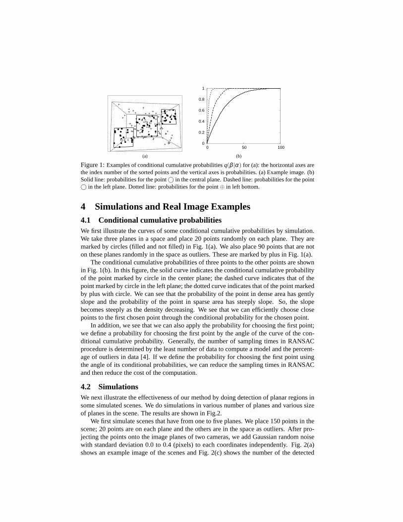
Figure 1:Examples of conditional cumulative probabilitiesq(β |α) for (a): the horizontal axes arethe index number of the sorted points and the vertical axes is probabilities. (a) Example image. (b)Solid line: probabilities for the point© in the central plane. Dashed line: probabilities for the point© in the left plane. Dotted line: probabilities for the point⊕ in left bottom.

4 Simulations and Real Image Examples4.1 Conditional cumulative probabilitiesWe first illustrate the curves of some conditional cumulative probabilities by simulation.We take three planes in a space and place 20 points randomly on each plane. They aremarked by circles (filled and not filled) in Fig. 1(a). We also place 90 points that are noton these planes randomly in the space as outliers. These are marked by plus in Fig. 1(a).

The conditional cumulative probabilities of three points to the other points are shownin Fig. 1(b). In this figure, the solid curve indicates the conditional cumulative probabilityof the point marked by circle in the center plane; the dashed curve indicates that of thepoint marked by circle in the left plane; the dotted curve indicates that of the point markedby plus with circle. We can see that the probability of the point in dense area has gentlyslope and the probability of the point in sparse area has steeply slope. So, the slopebecomes steeply as the density decreasing. We see that we can efficiently choose closepoints to the first chosen point through the conditional probability for the chosen point.

In addition, we see that we can also apply the probability for choosing the first point;we define a probability for choosing the first point by the angle of the curve of the con-ditional cumulative probability. Generally, the number of sampling times in RANSACprocedure is determined by the least number of data to compute a model and the percent-age of outliers in data [4]. If we define the probability for choosing the first point usingthe angle of its conditional probabilities, we can reduce the sampling times in RANSACand then reduce the cost of the computation.

4.2 SimulationsWe next illustrate the effectiveness of our method by doing detection of planar regions insome simulated scenes. We do simulations in various number of planes and various sizeof planes in the scene. The results are shown in Fig.2.

We first simulate scenes that have from one to five planes. We place 150 points in thescene; 20 points are on each plane and the others are in the space as outliers. After pro-jecting the points onto the image planes of two cameras, we add Gaussian random noisewith standard deviation 0.0 to 0.4 (pixels) to each coordinates independently. Fig. 2(a)shows an example image of the scenes and Fig. 2(c) shows the number of the detected

σ=0.0, proposed method

σ=0.2, proposed method

σ=0.4, proposed method

σ=0.0, standard RANSAC

σ=0.2, standard RANSAC

σ=0.4, standard RANSAC

(a) (b)

0

1

2

3

4

5

1 2 3 4 5 0

20

40

60

80

100

1 2 3 4 5 0

20

40

60

80

100

1 2 3 4 5

(c) (d) (e)

0

1

2

3

1/6 1/5 1/4 1/3 1/2 0

20

40

60

80

100

1/6 1/5 1/4 1/3 1/2 0

20

40

60

80

100

1/6 1/5 1/4 1/3 1/2

(f) (g) (h)

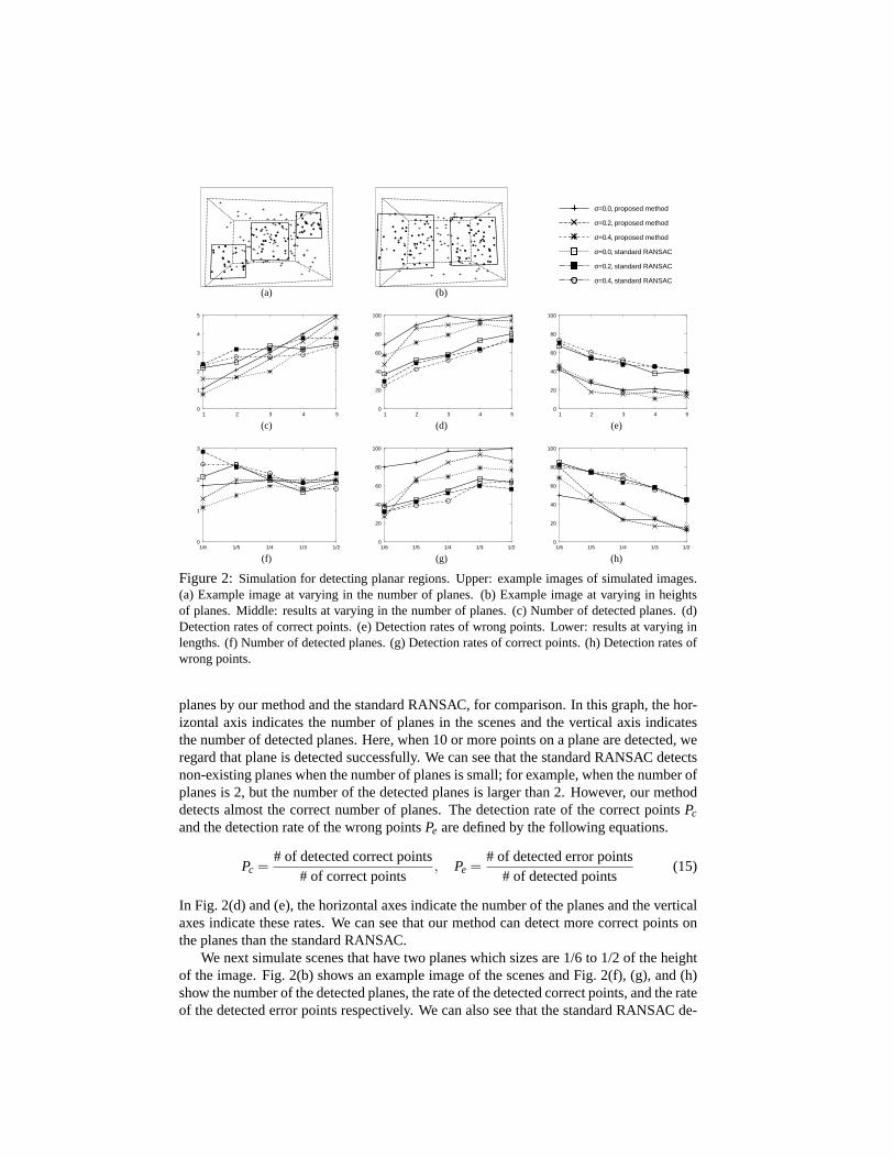
Figure 2:Simulation for detecting planar regions. Upper: example images of simulated images.(a) Example image at varying in the number of planes. (b) Example image at varying in heightsof planes. Middle: results at varying in the number of planes. (c) Number of detected planes. (d)Detection rates of correct points. (e) Detection rates of wrong points. Lower: results at varying inlengths. (f) Number of detected planes. (g) Detection rates of correct points. (h) Detection rates ofwrong points.

planes by our method and the standard RANSAC, for comparison. In this graph, the hor-izontal axis indicates the number of planes in the scenes and the vertical axis indicatesthe number of detected planes. Here, when 10 or more points on a plane are detected, weregard that plane is detected successfully. We can see that the standard RANSAC detectsnon-existing planes when the number of planes is small; for example, when the number ofplanes is 2, but the number of the detected planes is larger than 2. However, our methoddetects almost the correct number of planes. The detection rate of the correct pointsPc

and the detection rate of the wrong pointsPe are defined by the following equations.

Pc =# of detected correct points

# of correct points, Pe =

# of detected error points# of detected points

(15)

In Fig. 2(d) and (e), the horizontal axes indicate the number of the planes and the verticalaxes indicate these rates. We can see that our method can detect more correct points onthe planes than the standard RANSAC.

We next simulate scenes that have two planes which sizes are 1/6 to 1/2 of the heightof the image. Fig. 2(b) shows an example image of the scenes and Fig. 2(f), (g), and (h)show the number of the detected planes, the rate of the detected correct points, and the rateof the detected error points respectively. We can also see that the standard RANSAC de-

(a)

(b) (c) (d)

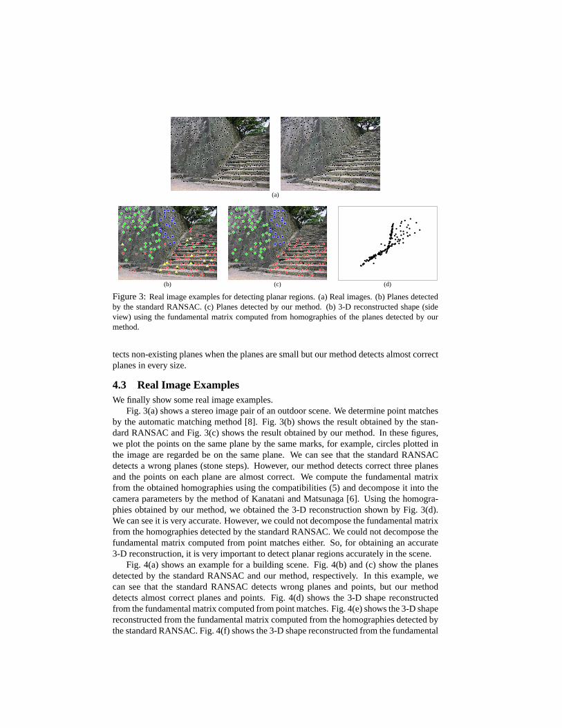
Figure 3:Real image examples for detecting planar regions. (a) Real images. (b) Planes detectedby the standard RANSAC. (c) Planes detected by our method. (b) 3-D reconstructed shape (sideview) using the fundamental matrix computed from homographies of the planes detected by ourmethod.

tects non-existing planes when the planes are small but our method detects almost correctplanes in every size.

4.3 Real Image ExamplesWe finally show some real image examples.

Fig. 3(a) shows a stereo image pair of an outdoor scene. We determine point matchesby the automatic matching method [8]. Fig. 3(b) shows the result obtained by the stan-dard RANSAC and Fig. 3(c) shows the result obtained by our method. In these figures,we plot the points on the same plane by the same marks, for example, circles plotted inthe image are regarded be on the same plane. We can see that the standard RANSACdetects a wrong planes (stone steps). However, our method detects correct three planesand the points on each plane are almost correct. We compute the fundamental matrixfrom the obtained homographies using the compatibilities (5) and decompose it into thecamera parameters by the method of Kanatani and Matsunaga [6]. Using the homogra-phies obtained by our method, we obtained the 3-D reconstruction shown by Fig. 3(d).We can see it is very accurate. However, we could not decompose the fundamental matrixfrom the homographies detected by the standard RANSAC. We could not decompose thefundamental matrix computed from point matches either. So, for obtaining an accurate3-D reconstruction, it is very important to detect planar regions accurately in the scene.

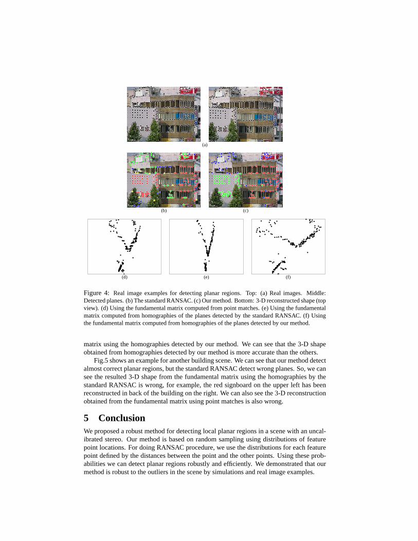
Fig. 4(a) shows an example for a building scene. Fig. 4(b) and (c) show the planesdetected by the standard RANSAC and our method, respectively. In this example, wecan see that the standard RANSAC detects wrong planes and points, but our methoddetects almost correct planes and points. Fig. 4(d) shows the 3-D shape reconstructedfrom the fundamental matrix computed from point matches. Fig. 4(e) shows the 3-D shapereconstructed from the fundamental matrix computed from the homographies detected bythe standard RANSAC. Fig. 4(f) shows the 3-D shape reconstructed from the fundamental

(a)

(b) (c)

(d) (e) (f)

Figure 4: Real image examples for detecting planar regions. Top: (a) Real images. Middle:Detected planes. (b) The standard RANSAC. (c) Our method. Bottom: 3-D reconstructed shape (topview). (d) Using the fundamental matrix computed from point matches. (e) Using the fundamentalmatrix computed from homographies of the planes detected by the standard RANSAC. (f) Usingthe fundamental matrix computed from homographies of the planes detected by our method.

matrix using the homographies detected by our method. We can see that the 3-D shapeobtained from homographies detected by our method is more accurate than the others.

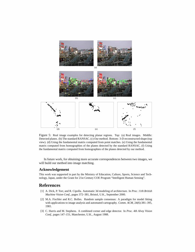
Fig.5 shows an example for another building scene. We can see that our method detectalmost correct planar regions, but the standard RANSAC detect wrong planes. So, we cansee the resulted 3-D shape from the fundamental matrix using the homographies by thestandard RANSAC is wrong, for example, the red signboard on the upper left has beenreconstructed in back of the building on the right. We can also see the 3-D reconstructionobtained from the fundamental matrix using point matches is also wrong.

5 ConclusionWe proposed a robust method for detecting local planar regions in a scene with an uncal-ibrated stereo. Our method is based on random sampling using distributions of featurepoint locations. For doing RANSAC procedure, we use the distributions for each featurepoint defined by the distances between the point and the other points. Using these prob-abilities we can detect planar regions robustly and efficiently. We demonstrated that ourmethod is robust to the outliers in the scene by simulations and real image examples.

(a)

(b) (c)

(d) (e) (f)

Figure 5: Real image examples for detecting planar regions. Top: (a) Real images. Middle:Detected planes. (b) The standard RANSAC. (c) Our method. Bottom: 3-D reconstructed shape (topview). (d) Using the fundamental matrix computed from point matches. (e) Using the fundamentalmatrix computed from homographies of the planes detected by the standard RANSAC. (f) Usingthe fundamental matrix computed from homographies of the planes detected by our method.

In future work, for obtaining more accurate correspondences between two images, wewill build our method into image matching.

AcknowledgementThis work was supported in part by the Ministry of Education, Culture, Sports, Science and Tech-nology, Japan, under the Grant for 21st Century COE Program “Intelligent Human Sensing”.

References[1] A. Dick, P. Torr, and R. Cipolla. Automatic 3d modeling of architecture. InProc. 11th British

Machine Vision Conf., pages 372–381, Bristol, U.K., September 2000.

[2] M.A. Fischler and R.C. Bolles. Random sample consensus: A paradigm for model fittingwith applications to image analysis and automated cartography.Comm. ACM, 24(6):381–395,1981.

[3] C. Harris and M. Stephens. A combined corner and edge detector. InProc. 4th Alvey VisionConf., pages 147–151, Manchester, U.K., August 1988.

[4] R. Hartley and A. Zisserman.Multiple View Geometry. Cambridge University press, Cam-bridge, 2000.

[5] K. Kanatani. Statistical Optimization for Geometric Computation: Theory and Practice. El-sevier Science, Amsterdam, 1996.

[6] K. Kanatani and C. Matsunaga. Closed-form expression for focal lengths from the fundamen-tal matrix. InProc. 4th Asian Conf. Comput. Vision, pages 128–133, Taipei, Taiwan, January2000.

[7] K. Kanatani, N. Ohta, and Y. Kanazawa. Optimal homography computation with a reliabilitymeasure.IEICE trans. Inf. & Syst., E83-D(7):1369–1374, June 2000.

[8] Y. Kanazawa and K. Kanatani. Robust image matching preserving global consistency. InProc. 6th Asian Conf. Comput. Vision, pages 1128–1133, Jeju Island, Korea, January 2004.

[9] Y. Kanazawa, T. Sakamoto, and H. Kawakami. Robust 3-d reconstruction using one or morehomographies with uncalibrated stereo. InProc. 6th Asian Conf. Comput. Vision, pages 503–508, Jeju Island, Korea, January 2004.

[10] Q.-T. Luong and O. Faugeras. Determining the fundamental matrix with planes: unstabilityand new algorithms. InProc. Comput. Vision Patt. Recog., pages 489–494, New York, U.S.A.,June 1993.

[11] J. Matas, O. Chum, M. Urban, and T. Pajdla. Robust wide baseline stereo from maximallystable extremal regions. InProc. 13th British Machine Vision Conf., pages 384–393, Cardiff,U.K., September 2002.

[12] P. J. Rousseeuw and A.M. Leroy.Robust Regression and Outlier Detection. Wiley, New York,1987.

[13] P.H.S. Torr and C. Davidson. Impsac: Synthesis of importance sampling and random sampleconsensus.IEEE Trans. Patt. Anal. Mach. Intel., 25(3):354–364, 2003.

[14] P.H.S. Torr and A. Zisserman. Robust computation and parameterization of multiple viewgeometry. InProc. 6th Int. Conf. Computer Vision, pages 727–732, Bombay, India, January1998.

[15] P.H.S. Torr and A. Zisserman. Mlesac: A new robust estimator with application to estimatingimage geometry.Comput. Vis. Image. Understand., 78:138–156, 2000.

[16] E. Trucco, F. Isgro, and F. Bracchi. Plane detection in disparity space. InProc. IEE Int. Conf.Visual Information Engineering, pages 73–76, Guildford, U.K., July 2003.

[17] Z. Zhang, R. Deriche, O. Faugeras, and Q.-T. Luong. A robust technique for matching twouncalibrated images through the recovery of the unknown epipolar geometry.Artif. Intell.,78:87–119, 1995.

[18] M. Zucchelli, J. Santos-Victor, and H.I. Christensen. Multiple plane segmentation using opti-cal flow. InProc. 13th British Machine Vision Conf., pages 313–322, Cardiff, U.K., September2002.