Embed Size (px)
Citation preview

Machine Vision and Applications (2021) 32:84https://doi.org/10.1007/s00138-021-01191-9
ORIG INAL PAPER
Segmentation of photovoltaic module cells in uncalibratedelectroluminescence images
Sergiu Deitsch1 · Claudia Buerhop-Lutz2 · Evgenii Sovetkin3 · Ansgar Steland4 · Andreas Maier5 ·Florian Gallwitz6 · Christian Riess7
Received: 6 August 2019 / Revised: 3 December 2020 / Accepted: 5 March 2021 / Published online: 24 May 2021© The Author(s) 2021, corrected publication 2021
AbstractHigh resolution electroluminescence (EL) images captured in the infrared spectrum allow to visually and non-destructivelyinspect the quality of photovoltaic (PV) modules. Currently, however, such a visual inspection requires trained experts todiscern different kinds of defects, which is time-consuming and expensive. Automated segmentation of cells is therefore akey step in automating the visual inspection workflow. In this work, we propose a robust automated segmentation methodfor extraction of individual solar cells from EL images of PV modules. This enables controlled studies on large amounts ofdata to understanding the effects of module degradation over time—a process not yet fully understood. The proposed methodinfers in several steps a high-level solar module representation from low-level ridge edge features. An important step in thealgorithm is to formulate the segmentation problem in terms of lens calibration by exploiting the plumbline constraint. Weevaluate our method on a dataset of various solar modules types containing a total of 408 solar cells with various defects. Ourmethod robustly solves this task with a median weighted Jaccard index of 94.47% and an F1 score of 97.62%, both indicatinga high sensitivity and a high similarity between automatically segmented and ground truth solar cell masks.
Keywords PV modules · EL imaging · Visual inspection · Lens distortion · Solar cell extraction · Pixelwise classification
B Sergiu [email protected]
Claudia [email protected]
Evgenii [email protected]
Ansgar [email protected]
Andreas [email protected]
Florian [email protected]
Christian [email protected]
1 Pattern Recognition Lab, Friedrich-Alexander UniversityErlangen-Nürnberg, Martensstr. 3, 91058 Erlangen, Germany
2 Helmholtz-Institut Erlangen-Nürnberg HI ERN,Forschungszentrum Jülich GmbH, Immerwahrstr. 2, 91058Erlangen, Germany
3 IEK5-Photovoltaik, Forschungszentrum Jülich GmbH, 52425Jülich, Germany
1 Introduction
Visual inspection of solar modules using EL imaging allowsto easily identify damage inflicted to solar panels either byenvironmental influences such as hail, during the assem-bly process, or due to prior material defects or materialaging [5,10,65,90,91,93]. The resulting defects can notablydecrease the photoelectric conversion efficiency of the mod-ules and thus their energy yield. This can be avoided bycontinuous inspection of solar modules and maintenanceof defective units. For an introduction and review of non-
4 Institute of Statistics, RWTH Aachen University,Wüllnerstr. 3, 52062 Aachen, Germany
5 Pattern Recognition Lab, Friedrich-Alexander UniversityErlangen-Nürnberg, Martensstr. 3, 91058 Erlangen, Germany
6 Faculty of Computer Science, Nuremberg Institute ofTechnology, Keßlerplatz 12, 90489 Nürnberg, Germany
7 IT Security Infrastructures Lab, Friedrich-AlexanderUniversity Erlangen-Nürnberg, Martensstr. 3, 91058Erlangen, Germany
123
84 Page 2 of 23 S. Deitsch et al.
automatic processing tools for EL images, we refer to Mauk[59].
An important step towards an automated visual inspectionis the segmentation of individual cells from the solar module.An accurate segmentation allows to extract spatially normal-ized solar cell images. We already used the proposed methodto develop a public dataset of solar cells images [12], whichare highly accurate training data for classifiers to predictdefects in solar modules [18,60]. In particular, the Convolu-tional Neural Network (CNN) training is greatly simplifiedwhen using spatially normalized samples, because CNNs aregenerally able to learn representations that are only equiv-ariant to small translations [35, pp. 335–336]. The learnedrepresentations, however, are not naturally invariant to otherspatial deformations such as rotation and scaling [35,44,52].
The identification of solar cells is additionally requiredby the international technical specification IEC TS 60904-13 [42, Annex D] for further identification of defects on celllevel. Automated segmentation can also ease the develop-ment of models that predict the performance of a PVmodulebased on detected or identified failure modes, or by deter-mining the operating voltage of each cell [70]. The datadescribing the cell characteristics can be fed into an elec-tric equivalent model that allows to estimate or simulate thecurrent-voltage characteristic (I-V) curve [13,46,72] or eventhe overall power output [47].
The appearance of PVmodules in EL images depends on anumber of different factors, which makes an automated seg-mentation challenging. The appearance varies with the typeof semiconducting material and with the shape of individualsolar cellwafers.Also, cell cracks and other defects can intro-ducedistracting streaks.A solar cell completely disconnectedfrom the electrical circuit will also appear much darker than afunctional cell. Additionally, solar modules vary in the num-ber of solar cells and their layout, and solar cells themselvesare oftentimes subdivided by busbars into multiple segmentsof different sizes. Therefore, it is desirable for a fully auto-mated segmentation to infer both the arrangement of solarcells within the PV module and their subdivision from ELimages alone, in a way that is robust to various disturbances.In particular, this may ease the inspection of heterogeneousbatches of PV modules.
In this work, we assume that EL images are captured ina manufacturing setting or under comparable conditions in atest laboratory where field-aged modules are analyzed eitherregularly or after hazards like hailstorms. Such laboratoriesoftentimes require agile work processes where the equip-ment is frequently remounted. In these scenarios, the ELirradiation of the solar module predominates the backgroundirradiation, and the solar modules are captured facing the ELcamera without major perspective distortion. Thus, the geo-metric distortions that are corrected by the proposed methodare radial lens distortion, in-plane rotation, and minor per-
spective distortions. This distinguishes the manufacturingsetting from acquisitions in the field, where PV modulesmay be occluded by cables and parts of the rack, and theperspective may be strong enough to require careful cor-rection. However, perspective distortion also makes it moredifficult to identify defective areas (e.g., microcracks) dueto the foreshortening effect [4]. Therefore, capturing ELimages from an extreme perspective is generally not advis-able. Specifically for manufacturing environments, however,the proposed method yields a robust, highly accurate, andcompletely automatic segmentation of solar modules intosolar cells from high resolution EL images of PV modules.
Independently of the setting, our goal is to allow for someflexibility for the user to freely position the camera or usezoom lenses without the need to recalibrate the camera.
With this goal in mind, a particular characteristic of theproposed segmentation pipeline is that it does not require anexternal calibration pattern. During the detection of the gridthat identifies individual solar cells, the busbars and the intersolar cell borders are directly used to estimate lens distortion.Avoiding the use of a separate calibration pattern also avoidsthe risk of an operator error during the calibration, e.g., dueto inexperienced personnel.
A robust and fully automatic PV module segmentationcan help understanding the influence of module degradationonmodule efficiency and power generation. Specifically, thisallows to continuously and automatically monitor the degra-dation process, for instance, by observing the differences ina series of solar cell images captured over a certain period oftime. The segmentation also allows to automatically createtraining data for learning-based algorithms for defect classi-fication and failure prediction.
1.1 Contributions
To the best of our knowledge, the proposed segmentationpipeline is the firstwork to enable a fully automatic extractionof solar cells from uncalibrated EL images of solar modules(cf., Fig. 1b). Within the pipeline, we seek to obtain the exactsegmentation mask of each solar cell through estimation ofnonlinear and linear transformations that warp the EL imageinto a canonical view. To this end, our contributions are three-fold:
1. Joint camera lens distortion estimation and PV modulegrid detection for precise solar cell region identification.
2. A robust initialization scheme for the employed lens dis-tortion model.
3. A highly accurate pixelwise classification into active solarcell area onmonocrystalline and polycrystalline PVmod-ules robust to various typical defects in solar modules.
123
Segmentation of photovoltaic module cells in uncalibrated electroluminescence... Page 3 of 23 84
Row
1
. . .
Row
2
. . .
. . .
(a) (b)
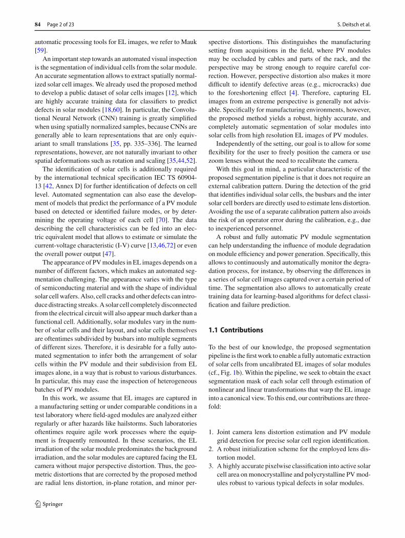
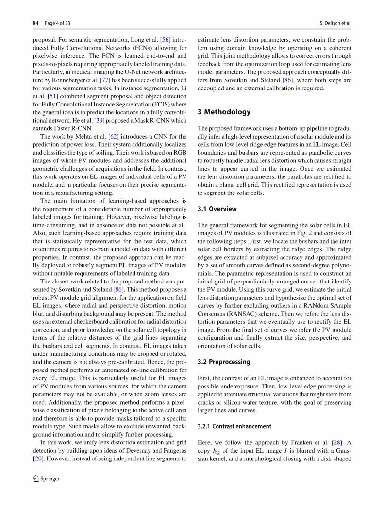
Fig. 1 (a) An EL image of a PV module overlaid by a rectangular grid ( ) and parabolic curve grid ( ) including the busbars ( )determined using our approach. The intersections of the rectangular grid were registered to curve grid intersections to accurately align both grids.Notice how the rectangular grid is still not able to capture the curved surface of the solar module induced by the (weak) lens distortion that increasesespecially towards the image border. Using the curve grid, we estimate the lens distortion, rectify the image and finally extract the individual cellsusing the estimated module topology (b). The segmented solar cells can be used for further analysis, such as automatic defect classification orfailure prediction in PV modules. The solar cells are approximately 15.6 cm× 15.6 cm with a standard 60 cell PV module with overall dimensionsof 1 m × 1.65 m
Moreover, our method operates on arbitrary (unseen)modulelayouts without prior knowledge on the layout.
1.2 Outline
The remainder of this work is organized as follows. Section2 discusses the related work. In Sect. 3, the individual stagesof the segmentation pipeline are presented. In Sect. 4, weevaluate the presented segmentation approach on a numberof different PV modules with respect to the segmentationaccuracy. Finally, the conclusions are given in Sect. 5.
2 Related work
The segmentation of PV modules into individual solar cellsis related to the detection of calibration patterns, such ascheckerboard patterns commonly used for calibrating intrin-sic camera and lens parameters [29,36,41,69,79]. However,the appearance of calibration patterns is typically perfectlyknown, whereas detection of solar cells is encumbered byvarious defects that are a priori unknown. Additionally, thenumber of solar cells in a PV module and their layout canvary.We also note that existing lensmodels generally assumewide angle lenses. However, their application to standardlenses is to our knowledge not widely studied.
To estimate the parameters of a lens distortion model,the plumbline constraint is typically employed [11]. The
constraint exploits the fact that the projection of straightlines under radial and tangential distortion will not be trulystraight. For example, under radial distortion, straight linesare images as curves. For typical visual inspection tasks,a single image is sufficient to estimate the lens distor-tion parameters [2,16,17,20,25,78]. This can be achieved bydecoupling the intrinsic parameters of the camera from theparameters of the lens distortion model [20].
Novel methodologies employ CNNs for various segmen-tation tasks. Existing CNN-based segmentation tasks canbe categorized into (1) object detection, (2) semantic seg-mentation, and (3) instance-aware segmentation. One of thefirst CNN object detection architectures is Regions withCNN features (R-CNN) [32] to learn features that are subse-quently classified using a class-specific linear Support VectorMachine (SVM) to generate region proposals. R-CNN learnsto simultaneously classify object proposals and refine theirspatial locations. The predicted regions, however, provideonly a coarse estimation of object’s location in terms ofbounding boxes. Girshick [31] proposed Fast Region-basedConvolutional Neural Network (Fast R-CNN) by acceler-ating training and testing times while also increasing thedetection accuracy. Ren et al. [75] introduced Region Pro-posal Network (RPN) that shares full-image convolutionalfeatures with the detection network enabling nearly cost-free region proposals. RPN is combined with Fast R-CNNinto a single network that simultaneously predicts objectbounds and estimates the probability of an object for each
123
84 Page 4 of 23 S. Deitsch et al.
proposal. For semantic segmentation, Long et al. [56] intro-duced Fully Convolutional Networks (FCNs) allowing forpixelwise inference. The FCN is learned end-to-end andpixels-to-pixels requiring appropriately labeled training data.Particularly, in medical imaging the U-Net network architec-ture by Ronneberger et al. [77] has been successfully appliedfor various segmentation tasks. In instance segmentation, Liet al. [51] combined segment proposal and object detectionfor FullyConvolutional Instance Segmentation (FCIS)wherethe general idea is to predict the locations in a fully convolu-tional network. He et al. [39] proposed aMaskR-CNNwhichextends Faster R-CNN.
The work by Mehta et al. [62] introduces a CNN for theprediction of power loss. Their system additionally localizesand classifies the type of soiling. Their work is based onRGBimages of whole PV modules and addresses the additionalgeometric challenges of acquisitions in the field. In contrast,this work operates on EL images of individual cells of a PVmodule, and in particular focuses on their precise segmenta-tion in a manufacturing setting.
The main limitation of learning-based approaches isthe requirement of a considerable number of appropriatelylabeled images for training. However, pixelwise labeling istime-consuming, and in absence of data not possible at all.Also, such learning-based approaches require training datathat is statistically representative for the test data, whichoftentimes requires to re-train a model on data with differentproperties. In contrast, the proposed approach can be read-ily deployed to robustly segment EL images of PV moduleswithout notable requirements of labeled training data.
The closest work related to the proposed method was pre-sented by Sovetkin and Steland [86]. This method proposes arobust PV module grid alignment for the application on fieldEL images, where radial and perspective distortion, motionblur, and disturbing backgroundmay be present. The methoduses an external checkerboard calibration for radial distortioncorrection, and prior knowledge on the solar cell topology interms of the relative distances of the grid lines separatingthe busbars and cell segments. In contrast, EL images takenunder manufacturing conditions may be cropped or rotated,and the camera is not always pre-calibrated. Hence, the pro-posed method performs an automated on-line calibration forevery EL image. This is particularly useful for EL imagesof PV modules from various sources, for which the cameraparameters may not be available, or when zoom lenses areused. Additionally, the proposed method performs a pixel-wise classification of pixels belonging to the active cell areaand therefore is able to provide masks tailored to a specificmodule type. Such masks allow to exclude unwanted back-ground information and to simplify further processing.
In this work, we unify lens distortion estimation and griddetection by building upon ideas of Devernay and Faugeras[20]. However, instead of using independent line segments to
estimate lens distortion parameters, we constrain the prob-lem using domain knowledge by operating on a coherentgrid. This joint methodology allows to correct errors throughfeedback from the optimization loop used for estimating lensmodel parameters. The proposed approach conceptually dif-fers from Sovetkin and Steland [86], where both steps aredecoupled and an external calibration is required.
3 Methodology
The proposed framework uses a bottom-up pipeline to gradu-ally infer a high-level representation of a solar module and itscells from low-level ridge edge features in an EL image. Cellboundaries and busbars are represented as parabolic curvesto robustly handle radial lens distortion which causes straightlines to appear curved in the image. Once we estimatedthe lens distortion parameters, the parabolas are rectified toobtain a planar cell grid. This rectified representation is usedto segment the solar cells.
3.1 Overview
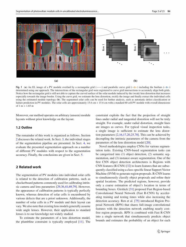
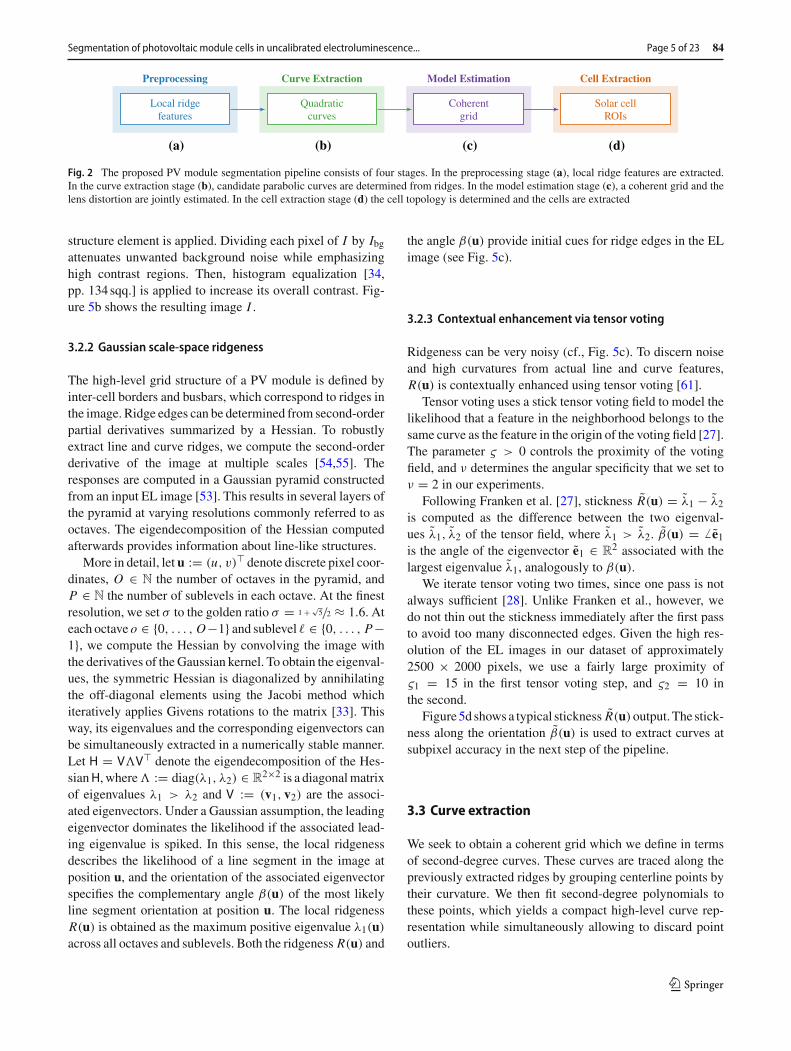
The general framework for segmenting the solar cells in ELimages of PV modules is illustrated in Fig. 2 and consists ofthe following steps. First, we locate the busbars and the intersolar cell borders by extracting the ridge edges. The ridgeedges are extracted at subpixel accuracy and approximatedby a set of smooth curves defined as second-degree polyno-mials. The parametric representation is used to construct aninitial grid of perpendicularly arranged curves that identifythe PV module. Using this curve grid, we estimate the initiallens distortion parameters and hypothesize the optimal set ofcurves by further excluding outliers in a RANdom SAmpleConsensus (RANSAC) scheme. Then we refine the lens dis-tortion parameters that we eventually use to rectify the ELimage. From the final set of curves we infer the PV moduleconfiguration and finally extract the size, perspective, andorientation of solar cells.
3.2 Preprocessing
First, the contrast of an EL image is enhanced to account forpossible underexposure. Then, low-level edge processing isapplied to attenuate structural variations thatmight stem fromcracks or silicon wafer texture, with the goal of preservinglarger lines and curves.
3.2.1 Contrast enhancement
Here, we follow the approach by Franken et al. [28]. Acopy Ibg of the input EL image I is blurred with a Gaus-sian kernel, and a morphological closing with a disk-shaped
123
Segmentation of photovoltaic module cells in uncalibrated electroluminescence... Page 5 of 23 84
Local ridgefeatures
Quadraticcurves
Coherentgrid
Solar cellROIs
(a) (b) (c) (d)
Preprocessing Curve Extraction Model Estimation Cell Extraction
Fig. 2 The proposed PV module segmentation pipeline consists of four stages. In the preprocessing stage (a), local ridge features are extracted.In the curve extraction stage (b), candidate parabolic curves are determined from ridges. In the model estimation stage (c), a coherent grid and thelens distortion are jointly estimated. In the cell extraction stage (d) the cell topology is determined and the cells are extracted
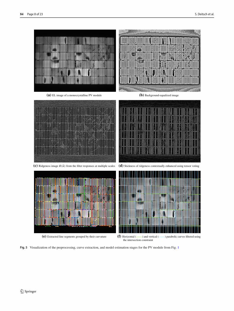
structure element is applied. Dividing each pixel of I by Ibgattenuates unwanted background noise while emphasizinghigh contrast regions. Then, histogram equalization [34,pp. 134sqq.] is applied to increase its overall contrast. Fig-ure 5b shows the resulting image I .
3.2.2 Gaussian scale-space ridgeness
The high-level grid structure of a PV module is defined byinter-cell borders and busbars, which correspond to ridges inthe image. Ridge edges can be determined from second-orderpartial derivatives summarized by a Hessian. To robustlyextract line and curve ridges, we compute the second-orderderivative of the image at multiple scales [54,55]. Theresponses are computed in a Gaussian pyramid constructedfrom an input EL image [53]. This results in several layers ofthe pyramid at varying resolutions commonly referred to asoctaves. The eigendecomposition of the Hessian computedafterwards provides information about line-like structures.
More in detail, let u := (u, v)� denote discrete pixel coor-dinates, O ∈ N the number of octaves in the pyramid, andP ∈ N the number of sublevels in each octave. At the finestresolution, we set σ to the golden ratio σ = 1 + √
5/2 ≈ 1.6. Ateach octave o ∈ {0, . . . , O−1} and sublevel � ∈ {0, . . . , P−1}, we compute the Hessian by convolving the image withthe derivatives of theGaussian kernel. To obtain the eigenval-ues, the symmetric Hessian is diagonalized by annihilatingthe off-diagonal elements using the Jacobi method whichiteratively applies Givens rotations to the matrix [33]. Thisway, its eigenvalues and the corresponding eigenvectors canbe simultaneously extracted in a numerically stable manner.Let H = V�V� denote the eigendecomposition of the Hes-sianH, where� := diag(λ1, λ2) ∈ R
2×2 is a diagonalmatrixof eigenvalues λ1 > λ2 and V := (v1, v2) are the associ-ated eigenvectors. Under a Gaussian assumption, the leadingeigenvector dominates the likelihood if the associated lead-ing eigenvalue is spiked. In this sense, the local ridgenessdescribes the likelihood of a line segment in the image atposition u, and the orientation of the associated eigenvectorspecifies the complementary angle β(u) of the most likelyline segment orientation at position u. The local ridgenessR(u) is obtained as the maximum positive eigenvalue λ1(u)
across all octaves and sublevels. Both the ridgeness R(u) and
the angle β(u) provide initial cues for ridge edges in the ELimage (see Fig. 5c).
3.2.3 Contextual enhancement via tensor voting
Ridgeness can be very noisy (cf., Fig. 5c). To discern noiseand high curvatures from actual line and curve features,R(u) is contextually enhanced using tensor voting [61].
Tensor voting uses a stick tensor voting field to model thelikelihood that a feature in the neighborhood belongs to thesame curve as the feature in the origin of the voting field [27].The parameter ς > 0 controls the proximity of the votingfield, and ν determines the angular specificity that we set toν = 2 in our experiments.
Following Franken et al. [27], stickness R(u) = λ1 − λ2is computed as the difference between the two eigenval-ues λ1, λ2 of the tensor field, where λ1 > λ2. β(u) = � e1is the angle of the eigenvector e1 ∈ R
2 associated with thelargest eigenvalue λ1, analogously to β(u).
We iterate tensor voting two times, since one pass is notalways sufficient [28]. Unlike Franken et al., however, wedo not thin out the stickness immediately after the first passto avoid too many disconnected edges. Given the high res-olution of the EL images in our dataset of approximately2500 × 2000 pixels, we use a fairly large proximity ofς1 = 15 in the first tensor voting step, and ς2 = 10 inthe second.
Figure 5d showsa typical stickness R(u)output. The stick-ness along the orientation β(u) is used to extract curves atsubpixel accuracy in the next step of the pipeline.
3.3 Curve extraction
We seek to obtain a coherent grid which we define in termsof second-degree curves. These curves are traced along thepreviously extracted ridges by grouping centerline points bytheir curvature. We then fit second-degree polynomials tothese points, which yields a compact high-level curve rep-resentation while simultaneously allowing to discard pointoutliers.
123
84 Page 6 of 23 S. Deitsch et al.
(b)(a)
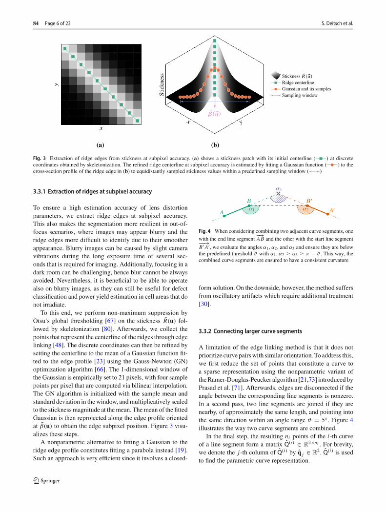
Fig. 3 Extraction of ridge edges from stickness at subpixel accuracy. (a) shows a stickness patch with its initial centerline ( ) at discretecoordinates obtained by skeletonization. The refined ridge centerline at subpixel accuracy is estimated by fitting a Gaussian function ( ) to thecross-section profile of the ridge edge in (b) to equidistantly sampled stickness values within a predefined sampling window ( )
3.3.1 Extraction of ridges at subpixel accuracy
To ensure a high estimation accuracy of lens distortionparameters, we extract ridge edges at subpixel accuracy.This also makes the segmentation more resilient in out-of-focus scenarios, where images may appear blurry and theridge edges more difficult to identify due to their smootherappearance. Blurry images can be caused by slight cameravibrations during the long exposure time of several sec-onds that is required for imaging. Additionally, focusing in adark room can be challenging, hence blur cannot be alwaysavoided. Nevertheless, it is beneficial to be able to operatealso on blurry images, as they can still be useful for defectclassification and power yield estimation in cell areas that donot irradiate.
To this end, we perform non-maximum suppression byOtsu’s global thresholding [67] on the stickness R(u) fol-lowed by skeletonization [80]. Afterwards, we collect thepoints that represent the centerline of the ridges through edgelinking [48]. The discrete coordinates can then be refined bysetting the centerline to the mean of a Gaussian function fit-ted to the edge profile [23] using the Gauss-Newton (GN)optimization algorithm [66]. The 1-dimensional window ofthe Gaussian is empirically set to 21 pixels, with four samplepoints per pixel that are computed via bilinear interpolation.The GN algorithm is initialized with the sample mean andstandard deviation in thewindow, andmultiplicatively scaledto the sticknessmagnitude at themean. Themean of the fittedGaussian is then reprojected along the edge profile orientedat β(u) to obtain the edge subpixel position. Figure 3 visu-alizes these steps.
A nonparametric alternative to fitting a Gaussian to theridge edge profile constitutes fitting a parabola instead [19].Such an approach is very efficient since it involves a closed-
1 2
3
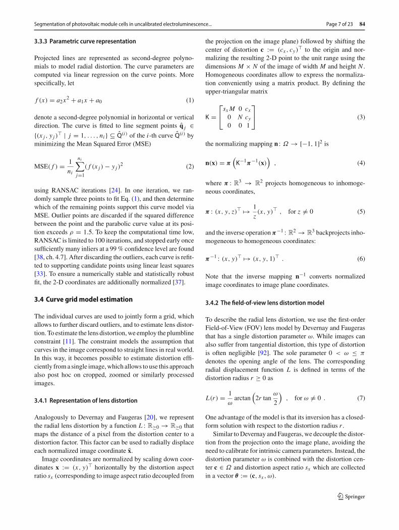
Fig. 4 When considering combining two adjacent curve segments, one
with the end line segment−→AB and the other with the start line segment−−→
B ′A′, we evaluate the angles α1, α2, and α3 and ensure they are belowthe predefined threshold ϑ with α1, α2 ≥ α3 ≥ π − ϑ . This way, thecombined curve segments are ensured to have a consistent curvature
form solution. On the downside, however, the method suffersfrom oscillatory artifacts which require additional treatment[30].
3.3.2 Connecting larger curve segments
A limitation of the edge linking method is that it does notprioritize curve pairswith similar orientation. To address this,we first reduce the set of points that constitute a curve toa sparse representation using the nonparametric variant oftheRamer-Douglas-Peucker algorithm [21,73] introduced byPrasad et al. [71]. Afterwards, edges are disconnected if theangle between the corresponding line segments is nonzero.In a second pass, two line segments are joined if they arenearby, of approximately the same length, and pointing intothe same direction within an angle range ϑ = 5◦. Figure 4illustrates the way two curve segments are combined.
In the final step, the resulting ni points of the i-th curveof a line segment form a matrix Q(i) ∈ R
2×ni . For brevity,we denote the j-th column of Q(i) by q j ∈ R
2. Q(i) is usedto find the parametric curve representation.
123
Segmentation of photovoltaic module cells in uncalibrated electroluminescence... Page 7 of 23 84
3.3.3 Parametric curve representation
Projected lines are represented as second-degree polyno-mials to model radial distortion. The curve parameters arecomputed via linear regression on the curve points. Morespecifically, let
f (x) = a2x2 + a1x + a0 (1)
denote a second-degree polynomial in horizontal or verticaldirection. The curve is fitted to line segment points q j ∈{(x j , y j )� | j = 1, . . . , ni } ⊆ Q(i) of the i-th curve Q(i) byminimizing the Mean Squared Error (MSE)
MSE( f ) = 1
ni
ni∑
j=1
( f (x j ) − y j )2 (2)
using RANSAC iterations [24]. In one iteration, we ran-domly sample three points to fit Eq. (1), and then determinewhich of the remaining points support this curve model viaMSE. Outlier points are discarded if the squared differencebetween the point and the parabolic curve value at its posi-tion exceeds ρ = 1.5. To keep the computational time low,RANSAC is limited to 100 iterations, and stopped early oncesufficiently many inliers at a 99% confidence level are found[38, ch. 4.7]. After discarding the outliers, each curve is refit-ted to supporting candidate points using linear least squares[33]. To ensure a numerically stable and statistically robustfit, the 2-D coordinates are additionally normalized [37].
3.4 Curve grid model estimation
The individual curves are used to jointly form a grid, whichallows to further discard outliers, and to estimate lens distor-tion. To estimate the lens distortion,we employ the plumblineconstraint [11]. The constraint models the assumption thatcurves in the image correspond to straight lines in real world.In this way, it becomes possible to estimate distortion effi-ciently froma single image,which allows to use this approachalso post hoc on cropped, zoomed or similarly processedimages.
3.4.1 Representation of lens distortion
Analogously to Devernay and Faugeras [20], we representthe radial lens distortion by a function L : R≥0 → R≥0 thatmaps the distance of a pixel from the distortion center to adistortion factor. This factor can be used to radially displaceeach normalized image coordinate x.
Image coordinates are normalized by scaling down coor-dinates x := (x, y)� horizontally by the distortion aspectratio sx (corresponding to image aspect ratio decoupled from
the projection on the image plane) followed by shifting thecenter of distortion c := (cx , cy)� to the origin and nor-malizing the resulting 2-D point to the unit range using thedimensions M × N of the image of width M and height N .Homogeneous coordinates allow to express the normaliza-tion conveniently using a matrix product. By defining theupper-triangular matrix
K =⎡
⎣sx M 0 cx0 N cy0 0 1
⎤
⎦ (3)
the normalizing mapping n : Ω → [−1, 1]2 is
n(x) = π(K−1π−1(x)
), (4)
where π : R3 → R
2 projects homogeneous to inhomoge-neous coordinates,
π : (x, y, z)� �→ 1
z(x, y)� , for z �= 0 (5)
and the inverse operationπ−1 : R2 → R
3 backprojects inho-mogeneous to homogeneous coordinates:
π−1 : (x, y)� �→ (x, y, 1)� . (6)
Note that the inverse mapping n−1 converts normalizedimage coordinates to image plane coordinates.
3.4.2 The field-of-view lens distortion model
To describe the radial lens distortion, we use the first-orderField-of-View (FOV) lens model by Devernay and Faugerasthat has a single distortion parameter ω. While images canalso suffer from tangential distortion, this type of distortionis often negligible [92]. The sole parameter 0 < ω ≤ π
denotes the opening angle of the lens. The correspondingradial displacement function L is defined in terms of thedistortion radius r ≥ 0 as
L(r) = 1
ωarctan
(2r tan
ω
2
), for ω �= 0 . (7)
One advantage of the model is that its inversion has a closed-form solution with respect to the distortion radius r .
Similar toDevernay and Faugeras, we decouple the distor-tion from the projection onto the image plane, avoiding theneed to calibrate for intrinsic camera parameters. Instead, thedistortion parameter ω is combined with the distortion cen-ter c ∈ Ω and distortion aspect ratio sx which are collectedin a vector θ := (c, sx , ω).
123
84 Page 8 of 23 S. Deitsch et al.
(a) EL image of a monocrystalline PV module (b) Background-equalized image
(c) Ridgeness image ( ) from the filter responses at multiple scales (d) Stickness of ridgeness contextually enhanced using tensor voting
(e) Extracted line segments grouped by their curvature (f) Horizontal ( ) and vertical ( ) parabolic curves filtered usingthe intersection constraint
Fig. 5 Visualization of the preprocessing, curve extraction, and model estimation stages for the PV module from Fig. 1
123
Segmentation of photovoltaic module cells in uncalibrated electroluminescence... Page 9 of 23 84
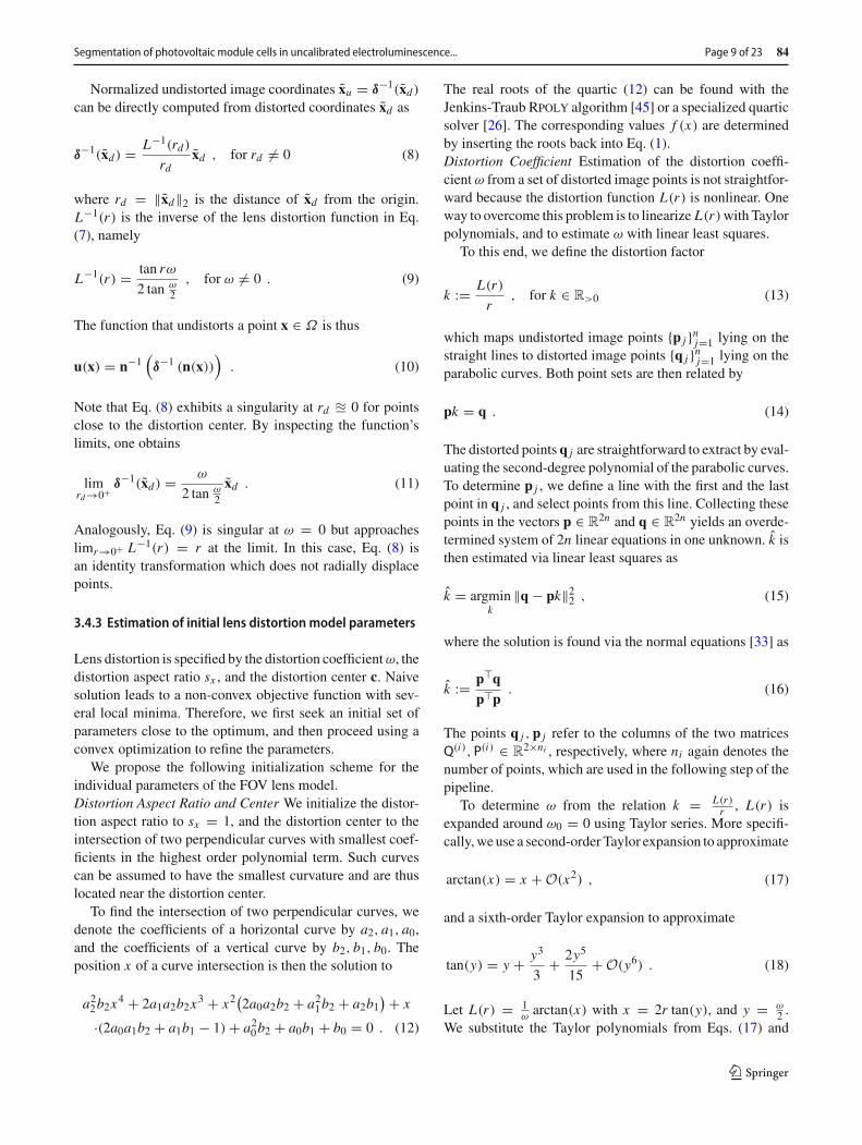
Normalized undistorted image coordinates xu = δ−1(xd)can be directly computed from distorted coordinates xd as
δ−1(xd) = L−1(rd)
rdxd , for rd �= 0 (8)
where rd = ‖xd‖2 is the distance of xd from the origin.L−1(r) is the inverse of the lens distortion function in Eq.(7), namely
L−1(r) = tan rω
2 tan ω2
, for ω �= 0 . (9)
The function that undistorts a point x ∈ Ω is thus
u(x) = n−1(δ−1 (n(x))
). (10)
Note that Eq. (8) exhibits a singularity at rd � 0 for pointsclose to the distortion center. By inspecting the function’slimits, one obtains
limrd→0+ δ−1(xd) = ω
2 tan ω2
xd . (11)
Analogously, Eq. (9) is singular at ω = 0 but approacheslimr→0+ L−1(r) = r at the limit. In this case, Eq. (8) isan identity transformation which does not radially displacepoints.
3.4.3 Estimation of initial lens distortion model parameters
Lens distortion is specified by the distortion coefficientω, thedistortion aspect ratio sx , and the distortion center c. Naivesolution leads to a non-convex objective function with sev-eral local minima. Therefore, we first seek an initial set ofparameters close to the optimum, and then proceed using aconvex optimization to refine the parameters.
We propose the following initialization scheme for theindividual parameters of the FOV lens model.Distortion Aspect Ratio and Center We initialize the distor-tion aspect ratio to sx = 1, and the distortion center to theintersection of two perpendicular curves with smallest coef-ficients in the highest order polynomial term. Such curvescan be assumed to have the smallest curvature and are thuslocated near the distortion center.
To find the intersection of two perpendicular curves, wedenote the coefficients of a horizontal curve by a2, a1, a0,and the coefficients of a vertical curve by b2, b1, b0. Theposition x of a curve intersection is then the solution to
a22b2x4 + 2a1a2b2x
3 + x2(2a0a2b2 + a21b2 + a2b1
) + x
·(2a0a1b2 + a1b1 − 1) + a20b2 + a0b1 + b0 = 0 . (12)
The real roots of the quartic (12) can be found with theJenkins-Traub Rpoly algorithm [45] or a specialized quarticsolver [26]. The corresponding values f (x) are determinedby inserting the roots back into Eq. (1).Distortion Coefficient Estimation of the distortion coeffi-cientω from a set of distorted image points is not straightfor-ward because the distortion function L(r) is nonlinear. Oneway to overcome this problem is to linearize L(r)with Taylorpolynomials, and to estimate ω with linear least squares.
To this end, we define the distortion factor
k := L(r)
r, for k ∈ R>0 (13)
which maps undistorted image points {p j }nj=1 lying on thestraight lines to distorted image points {q j }nj=1 lying on theparabolic curves. Both point sets are then related by
pk = q . (14)
The distorted points q j are straightforward to extract by eval-uating the second-degree polynomial of the parabolic curves.To determine p j , we define a line with the first and the lastpoint in q j , and select points from this line. Collecting thesepoints in the vectors p ∈ R
2n and q ∈ R2n yields an overde-
termined system of 2n linear equations in one unknown. k isthen estimated via linear least squares as
k = argmink
‖q − pk‖22 , (15)
where the solution is found via the normal equations [33] as
k := p�qp�p
. (16)
The points q j ,p j refer to the columns of the two matricesQ(i), P(i) ∈ R
2×ni , respectively, where ni again denotes thenumber of points, which are used in the following step of thepipeline.
To determine ω from the relation k = L(r)r , L(r) is
expanded around ω0 = 0 using Taylor series. More specifi-cally,we use a second-order Taylor expansion to approximate
arctan(x) = x + O(x2) , (17)
and a sixth-order Taylor expansion to approximate
tan(y) = y + y3
3+ 2y5
15+ O(y6) . (18)
Let L(r) = 1ωarctan(x) with x = 2r tan(y), and y = ω
2 .We substitute the Taylor polynomials from Eqs. (17) and
123
84 Page 10 of 23 S. Deitsch et al.
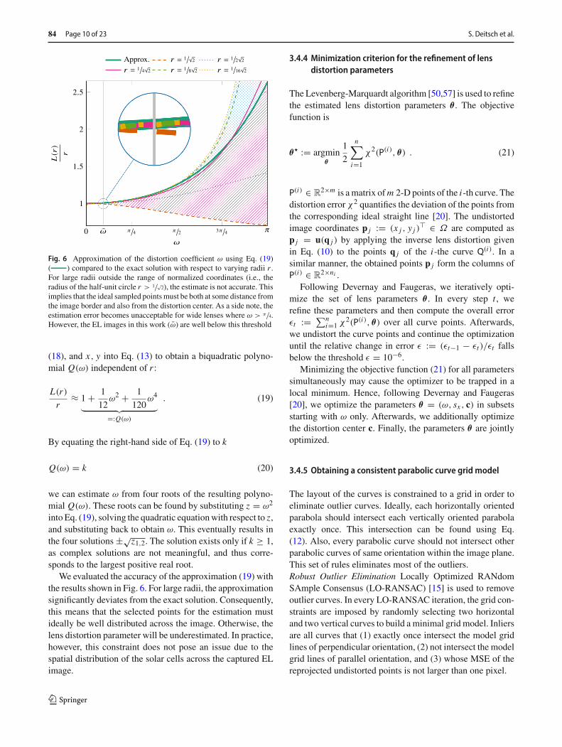
Fig. 6 Approximation of the distortion coefficient ω using Eq. (19)( ) compared to the exact solution with respect to varying radii r .For large radii outside the range of normalized coordinates (i.e., theradius of the half-unit circle r > 1/
√2), the estimate is not accurate. This
implies that the ideal sampled pointsmust be both at some distance fromthe image border and also from the distortion center. As a side note, theestimation error becomes unacceptable for wide lenses where ω > π/4.However, the EL images in this work (ω) are well below this threshold
(18), and x, y into Eq. (13) to obtain a biquadratic polyno-mial Q(ω) independent of r :
L(r)
r≈ 1 + 1
12ω2 + 1
120ω4
︸ ︷︷ ︸=:Q(ω)
. (19)
By equating the right-hand side of Eq. (19) to k
Q(ω) = k (20)
we can estimate ω from four roots of the resulting polyno-mial Q(ω). These roots can be found by substituting z = ω2
into Eq. (19), solving the quadratic equationwith respect to z,and substituting back to obtain ω. This eventually results inthe four solutions ±√
z1,2. The solution exists only if k ≥ 1,as complex solutions are not meaningful, and thus corre-sponds to the largest positive real root.
We evaluated the accuracy of the approximation (19) withthe results shown in Fig. 6. For large radii, the approximationsignificantly deviates from the exact solution. Consequently,this means that the selected points for the estimation mustideally be well distributed across the image. Otherwise, thelens distortion parameter will be underestimated. In practice,however, this constraint does not pose an issue due to thespatial distribution of the solar cells across the captured ELimage.
3.4.4 Minimization criterion for the refinement of lensdistortion parameters
The Levenberg-Marquardt algorithm [50,57] is used to refinethe estimated lens distortion parameters θ . The objectivefunction is
θ� := argminθ
1
2
n∑
i=1
χ2(P(i), θ) . (21)
P(i) ∈ R2×m is amatrix ofm 2-D points of the i-th curve. The
distortion error χ2 quantifies the deviation of the points fromthe corresponding ideal straight line [20]. The undistortedimage coordinates p j := (x j , y j )� ∈ Ω are computed asp j = u(q j ) by applying the inverse lens distortion givenin Eq. (10) to the points q j of the i-the curve Q(i). In asimilar manner, the obtained points p j form the columns ofP(i) ∈ R
2×ni .Following Devernay and Faugeras, we iteratively opti-
mize the set of lens parameters θ . In every step t , werefine these parameters and then compute the overall errorεt := ∑n
i=1 χ2(P(i), θ) over all curve points. Afterwards,we undistort the curve points and continue the optimizationuntil the relative change in error ε := (εt−1 − εt )/εt fallsbelow the threshold ε = 10−6.
Minimizing the objective function (21) for all parameterssimultaneously may cause the optimizer to be trapped in alocal minimum. Hence, following Devernay and Faugeras[20], we optimize the parameters θ = (ω, sx , c) in subsetsstarting with ω only. Afterwards, we additionally optimizethe distortion center c. Finally, the parameters θ are jointlyoptimized.
3.4.5 Obtaining a consistent parabolic curve grid model
The layout of the curves is constrained to a grid in order toeliminate outlier curves. Ideally, each horizontally orientedparabola should intersect each vertically oriented parabolaexactly once. This intersection can be found using Eq.(12). Also, every parabolic curve should not intersect otherparabolic curves of same orientation within the image plane.This set of rules eliminates most of the outliers.Robust Outlier Elimination Locally Optimized RANdomSAmple Consensus (LO-RANSAC) [15] is used to removeoutlier curves. In every LO-RANSAC iteration, the grid con-straints are imposed by randomly selecting two horizontaland two vertical curves to build a minimal grid model. Inliersare all curves that (1) exactly once intersect the model gridlines of perpendicular orientation, (2) not intersect the modelgrid lines of parallel orientation, and (3) whose MSE of thereprojected undistorted points is not larger than one pixel.
123
Segmentation of photovoltaic module cells in uncalibrated electroluminescence... Page 11 of 23 84
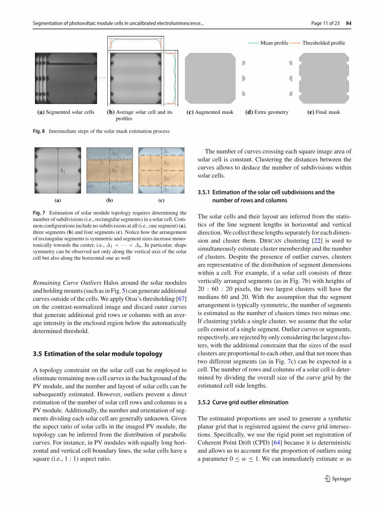
Fig. 8 Intermediate steps of the solar mask estimation process
Δ1
(a)
Δ1
Δ1
Δ2
(b)
Δ1
Δ1
Δ2
Δ2
(c)
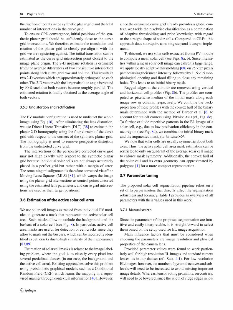
Fig. 7 Estimation of solar module topology requires determining thenumber of subdivisions (i.e., rectangular segments) in a solar cell. Com-mon configurations include no subdivisions at all (i.e., one segment) (a),three segments (b) and four segments (c). Notice how the arrangementof rectangular segments is symmetric and segment sizes increasemono-tonically towards the center, i.e., Δ1 < · · · < Δn . In particular, shapesymmetry can be observed not only along the vertical axis of the solarcell but also along the horizontal one as well
Remaining Curve Outliers Halos around the solar modulesand holdingmounts (such as in Fig. 5) can generate additionalcurves outside of the cells.We applyOtsu’s thresholding [67]on the contrast-normalized image and discard outer curvesthat generate additional grid rows or columns with an aver-age intensity in the enclosed region below the automaticallydetermined threshold.
3.5 Estimation of the solar module topology
A topology constraint on the solar cell can be employed toeliminate remaining non-cell curves in the background of thePV module, and the number and layout of solar cells can besubsequently estimated. However, outliers prevent a directestimation of the number of solar cell rows and columns in aPVmodule. Additionally, the number and orientation of seg-ments dividing each solar cell are generally unknown. Giventhe aspect ratio of solar cells in the imaged PV module, thetopology can be inferred from the distribution of paraboliccurves. For instance, in PV modules with equally long hori-zontal and vertical cell boundary lines, the solar cells have asquare (i.e., 1 : 1) aspect ratio.
The number of curves crossing each square image area ofsolar cell is constant. Clustering the distances between thecurves allows to deduce the number of subdivisions withinsolar cells.
3.5.1 Estimation of the solar cell subdivisions and thenumber of rows and columns
The solar cells and their layout are inferred from the statis-tics of the line segment lengths in horizontal and verticaldirection.We collect these lengths separately for each dimen-sion and cluster them. Dbscan clustering [22] is used tosimultaneously estimate cluster membership and the numberof clusters. Despite the presence of outlier curves, clustersare representative of the distribution of segment dimensionswithin a cell. For example, if a solar cell consists of threevertically arranged segments (as in Fig. 7b) with heights of20 : 60 : 20 pixels, the two largest clusters will have themedians 60 and 20. With the assumption that the segmentarrangement is typically symmetric, the number of segmentsis estimated as the number of clusters times two minus one.If clustering yields a single cluster, we assume that the solarcells consist of a single segment. Outlier curves or segments,respectively, are rejected by only considering the largest clus-ters, with the additional constraint that the sizes of the usedclusters are proportional to each other, and that not more thantwo different segments (as in Fig. 7c) can be expected in acell. The number of rows and columns of a solar cell is deter-mined by dividing the overall size of the curve grid by theestimated cell side lengths.
3.5.2 Curve grid outlier elimination
The estimated proportions are used to generate a syntheticplanar grid that is registered against the curve grid intersec-tions. Specifically, we use the rigid point set registration ofCoherent Point Drift (CPD) [64] because it is deterministicand allows us to account for the proportion of outliers usinga parameter 0 ≤ w ≤ 1. We can immediately estimate w as
123
84 Page 12 of 23 S. Deitsch et al.
the fraction of points in the synthetic planar grid and the totalnumber of intersections in the curve grid.
To ensure CPD convergence, initial positions of the syn-thetic planar grid should be sufficiently close to the curvegrid intersections. We therefore estimate the translation androtation of the planar grid to closely pre-align it with thegrid we are registering against. The initial translation can beestimated as the curve grid intersection point closest to theimage plane origin. The 2-D in-plane rotation is estimatedfrom the average differences of two consecutive intersectionpoints along each curve grid row and column. This results intwo 2-D vectors which are approximately orthogonal to eachother. The 2-D vector with the larger absolute angle is rotatedby 90 % such that both vectors become roughly parallel. Theestimated rotation is finally obtained as the average angle ofboth vectors.
3.5.3 Undistortion and rectification
The PV module configuration is used to undistort the wholeimage using Eq. (10). After eliminating the lens distortion,we use Direct Linear Transform (DLT) [38] to estimate theplanar 2-D homography using the four corners of the curvegrid with respect to the corners of the synthetic planar grid.The homography is used to remove perspective distortionfrom the undistorted curve grid.
The intersections of the perspective corrected curve gridmay not align exactly with respect to the synthetic planargrid because individual solar cells are not always accuratelyplaced in a perfect grid but rather with a margin of error.The remaining misalignment is therefore corrected via affineMoving Least Squares (MLS) [81], which warps the imageusing the planar grid intersections as control points distortedusing the estimated lens parameters, and curve grid intersec-tions are used as their target positions.
3.6 Estimation of the active solar cell area
We use solar cell images extracted from individual PV mod-ules to generate a mask that represents the active solar cellarea. Such masks allow to exclude the background and thebusbars of a solar cell (see Fig. 8). In particular, active cellarea masks are useful for detection of cell cracks since theyallow to mask out the busbars, which can be incorrectly iden-tified as cell cracks due to high similarity of their appearance[87,89].
Estimation of solar cellmasks is related to the image label-ing problem, where the goal is to classify every pixel intoseveral predefined classes (in our case, the background andthe active cell area). Existing approaches solve this problemusing probabilistic graphical models, such as a ConditionalRandom Field (CRF) which learns the mapping in a super-visedmanner through contextual information [40]. However,
since the estimated curve grid already provides a global con-text, we tackle the pixelwise classification as a combinationof adaptive thresholding and prior knowledge with regardto the straight shape of solar cells. Compared to CRFs, thisapproach does not require a training step and is easy to imple-ment.
To this end, we use solar cells extracted from a PVmoduleto compute a mean solar cell (see Figs. 8a, b). Since intensi-ties within a mean solar cell image can exhibit a large range,we apply locally adaptive thresholding [68] on 25×25 pixelspatches using theirmean intensity, followed by a 15×15mor-phological opening and flood filling to close any remainingholes. This leads to an initial binary mask.
Ragged edges at the contour are removed using verticaland horizontal cell profiles (Fig. 8b). The profiles are com-puted as pixelwise median of the initial mask along eachimage row or column, respectively. We combine the back-projection of these profiles with the convex hull of the binarymask determined with the method of Barber et al. [6] toaccount for cut-off corners using bitwise AND (cf., Fig. 8c).To further exclude repetitive patterns in the EL image of asolar cell, e.g., due to low passivation efficiency in the con-tact region (see Fig. 8d), we combine the initial binary maskand the augmented mask via bitwise XOR.
We note that solar cells are usually symmetric about bothaxes. Thus, the active solar cell area mask estimation can berestricted to only on quadrant of the average solar cell imageto enforce mask symmetry. Additionally, the convex hull ofthe solar cell and its extra geometry can approximated bypolygons [1] for a more compact representation.
3.7 Parameter tuning
The proposed solar cell segmentation pipeline relies on aset of hyperparameters that directly affect the segmentationrobustness and accuracy. Table 1 provides an overview of allparameters with their values used in this work.
3.7.1 Manual search
Since the parameters of the proposed segmentation are intu-itive and easily interpretable, it is straightforward to selectthem based on the setup used for EL image acquisition.
Main influence factors that must be considered whenchoosing the parameters are image resolution and physicalproperties of the camera lens.
Provided parameter values were found to work particu-larly well for high resolution EL images and standard cameralenses, as in our dataset (cf., Sect. 4.1). For low resolutionEL images, however, the number of pyramid octaves and sub-levels will need to be increased to avoid missing importantimage details.Whereas, tensor voting proximity, on contrary,will need to be lowered, since the width of ridge edges in low
123
Segmentation of photovoltaic module cells in uncalibrated electroluminescence... Page 13 of 23 84
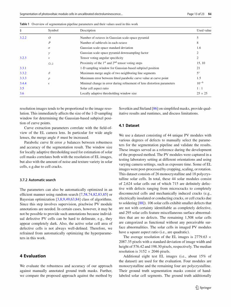
Table 1 Overview of segmentation pipeline parameters and their values used in this work
§ Symbol Description Used value
3.2.2 O Number of octaves in Gaussian scale-space pyramid 5
P Number of sublevels in each octave 8
σ Gaussian scale-space standard deviation 1.6
γ Gaussian scale-space pyramid downsampling factor 2
3.2.3 ν Tensor voting angular specificity 2
ς1,2 Proximity of the 1st and 2nd tensor voting steps 15, 10
3.3.1 1-D sampling window for Gaussian-based subpixel position 21
3.3.2 ϑ Maximum merge angle of two neighboring line segments 5◦
3.3.3 ρ Maximum error between fitted parabolic curve value at curve point 1.5
3.4.4 ε Minimal change in error during refinement of lens distortion parameters 10−6
3.5 Solar cell aspect ratio 1 : 13.6 Locally adaptive thresholding window size 25 × 25
resolution images tends to be proportional to the image reso-lution. This immediately affects the size of the 1-D samplingwindow for determining the Gaussian-based subpixel posi-tion of curve points.
Curve extraction parameters correlate with the field-of-view of the EL camera lens. In particular for wide anglelenses, the merge angle ϑ must be increased.
Parabolic curve fit error ρ balances between robustnessand accuracy of the segmentation result. The window sizefor locally adaptive thresholding used for estimation of solarcell masks correlates both with the resolution of EL images,but also with the amount of noise and texture variety in solarcells, e.g.due to cell cracks.
3.7.2 Automatic search
The parameters can also be automatically optimized in anefficient manner using random search [7,58,74,82,83,85] orBayesian optimization [3,8,9,49,63,84] class of algorithms.Since this step involves supervision, pixelwise PV moduleannotations are needed. In certain cases, however, it may benot be possible to provide such annotations because individ-ual defective PV cells can be hard to delineate, e.g., theyappear completely dark. Also, the active solar cell area ofdefective cells is not always well-defined. Therefore, werefrained from automatically optimizing the hyperparame-ters in this work.
4 Evaluation
We evaluate the robustness and accuracy of our approachagainst manually annotated ground truth masks. Further,we compare the proposed approach against the method by
Sovetkin and Steland [86] on simplifiedmasks, provide qual-itative results and runtimes, and discuss limitations.
4.1 Dataset
We use a dataset consisting of 44 unique PV modules withvarious degrees of defects to manually select the parame-ters for the segmentation pipeline and validate the results.These images served as a reference during the developmentof the proposed method. The PV modules were captured in atesting laboratory setting at different orientations and usingvarying camera settings, such as exposure time. Some of ELimageswere post-processed by cropping, scaling, or rotation.This dataset consists of 26 monocrystalline and 18 polycrys-talline solar cells. In total, these 44 solar modules consistof 2,624 solar cells out of which 715 are definitely defec-tive with defects ranging from microcracks to completelydisconnected cells and mechanically induced cracks (e.g.,electrically insulated or conducting cracks, or cell cracks dueto soldering [88]). 106 solar cells exhibit smaller defects thatare not with certainty identifiable as completely defective,and 295 solar cells feature miscellaneous surface abnormal-ities that are no defects. The remaining 1,508 solar cellsare categorized as functional without any perceivable sur-face abnormalities. The solar cells in imaged PV moduleshave a square aspect ratio (i.e., are quadratic).
The average resolution of the EL images is 2779.63 ×2087.35 pixels with a standard deviation of image width andheight of 576.42 and 198.30 pixels, respectively. The medianresolution is 3152 × 2046 pixels.
Additional eight test EL images (i.e., about 15% ofthe dataset) are used for the evaluation. Four modules aremonocrystalline and the remaining four are polycrystalline.Their ground truth segmentation masks consist of hand-labeled solar cell segments. The ground truth additionally
123
84 Page 14 of 23 S. Deitsch et al.
specifies both the rows and columns of the solar cells, andtheir subdivisions. These images show various PV moduleswith a total of 408 solar cells. The resolution of the test ELimages varies around 2649.50 ± 643.20 × 2074 ± 339.12with a median image resolution of 2581.50 × 2046.
Three out of four monocrystalline modules consist of 4×9 cells and the remaining monocrystalline module consistsof 6 × 10 cells. All of their cells are subdivided by busbarsinto 3 × 1 segments.
The polycrystalline modules consist of 6 × 10 solar cellseach. In two of the modules, every cell is subdivided into 3×1 segments. The cells of the other twomodules are subdividedinto 4 × 1 segments.
4.2 Evaluationmetrics
We use two different metrics, pixelwise scores and theweighted Jaccard index to evaluate both the robustness andthe accuracy of the proposed method and to compare ourmethod against related work. In the latter case, we addition-ally use a third metric, the Root Mean Square Error (RMSE),to compute the segmentation error on simplified masks.
4.2.1 Root mean square error
The first performance metric is the RMSE given in pixelsbetween the corners of the quadrilateralmask computed fromthe ground truth annotations and the corners estimated by theindividual modalities. The metric provides a summary of themethod’s accuracy in absolute terms across all experiments.
4.2.2 Pixelwise classification
The second set of performance metrics are precision, recall,and the F1 score [76]. These metrics are computed byconsidering cell segmentation as a multiclass pixelwise clas-sification into background and active area of individual solarcells. A typical 60 cell PV module will therefore contain upto 61 class labels. A correctly segmented active area pixel isa true positive, the remaining quantities are defined accord-ingly. Pixelwise scores are computed globally with respectto all the pixels. Therefore, the differences between the indi-vidual results for these scores are naturally smaller than formetrics that are computed with respect to individual solarcells, such as the Jaccard index.
4.2.3 Weighted Jaccard Index
The third performance metric is the weighted Jaccard index[14,43], a variant of themetric widely known as Intersection-over-Union (IoU). This metric extends the common Jaccardindex by an importance weighting of the input pixels. Asthe compared masks are not strictly binary either due to
antialiasing or interpolation during mask construction, wedefine importance of pixels by their intensity. Given two non-binary masks A and B, the weighted Jaccard similarity is
Jw =∑
u∈Ω min{A(u), B(u)}∑u∈Ω max{A(u), B(u)} . (22)
The performance metric is computed on pairs of segmentedcells and ground truth masks. A ground truth cell mask ismatched to the segmented cell with the largest intersectionarea, thus taking structural coherence into account.
We additionally compute the Jaccard index of the back-ground, which corresponds to the accuracy of the method tosegment the whole solar module. Solar cell misalignment ormissed cells will therefore penalize the segmentation accu-racy to a high degree. Therefore, the solar module Jaccardindex provides a summary of howwell the segmentation per-forms per EL image.
4.3 Quantitative results
We evaluate the segmentation accuracy and the robustness ofour approach using a fixed set of parameters as specified inTable 1 on EL images of PV modules acquired in a materialtesting laboratory.
4.3.1 Comparison to related work with simplified cell masks
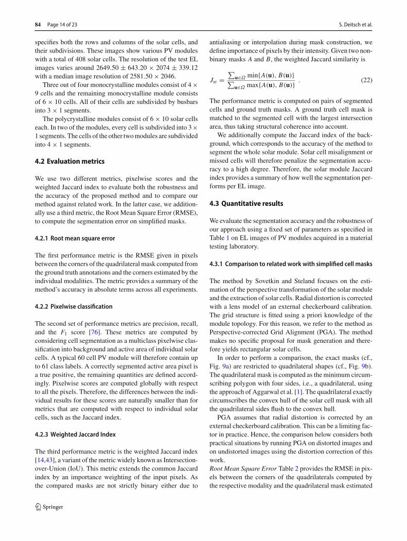
The method by Sovetkin and Steland focuses on the esti-mation of the perspective transformation of the solar moduleand the extraction of solar cells. Radial distortion is correctedwith a lens model of an external checkerboard calibration.The grid structure is fitted using a priori knowledge of themodule topology. For this reason, we refer to the method asPerspective-corrected Grid Alignment (PGA). The methodmakes no specific proposal for mask generation and there-fore yields rectangular solar cells.
In order to perform a comparison, the exact masks (cf.,Fig. 9a) are restricted to quadrilateral shapes (cf., Fig. 9b).The quadrilateral mask is computed as the minimum circum-scribing polygon with four sides, i.e., a quadrilateral, usingthe approach of Aggarwal et al. [1]. The quadrilateral exactlycircumscribes the convex hull of the solar cell mask with allthe quadrilateral sides flush to the convex hull.
PGA assumes that radial distortion is corrected by anexternal checkerboard calibration. This can be a limiting fac-tor in practice. Hence, the comparison below considers bothpractical situations by running PGA on distorted images andon undistorted images using the distortion correction of thiswork.Root Mean Square Error Table 2 provides the RMSE in pix-els between the corners of the quadrilaterals computed bythe respective modality and the quadrilateral mask estimated
123
Segmentation of photovoltaic module cells in uncalibrated electroluminescence... Page 15 of 23 84
Fig. 9 Example of an exact mask (a) of solar cells estimated using the proposed approach and a quadrilateral mask (b) determined from the exactmask. The latter is used for comparison against the method of Sovetkin and Steland [86]. Both masks are shown as color overlays. Different colorsdenote different instances of solar cells
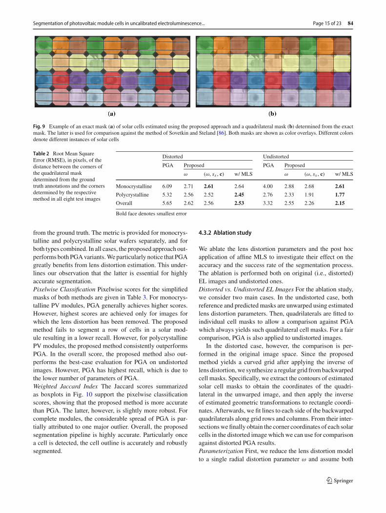
Table 2 Root Mean SquareError (RMSE), in pixels, of thedistance between the corners ofthe quadrilateral maskdetermined from the groundtruth annotations and the cornersdetermined by the respectivemethod in all eight test images
Distorted Undistorted
PGA Proposed PGA Proposed
ω (ω, sx , c) w/ MLS ω (ω, sx , c) w/ MLS
Monocrystalline 6.09 2.71 2.61 2.64 4.00 2.88 2.68 2.61
Polycrystalline 5.32 2.56 2.52 2.45 2.76 2.33 1.91 1.77
Overall 5.65 2.62 2.56 2.53 3.32 2.55 2.26 2.15
Bold face denotes smallest error
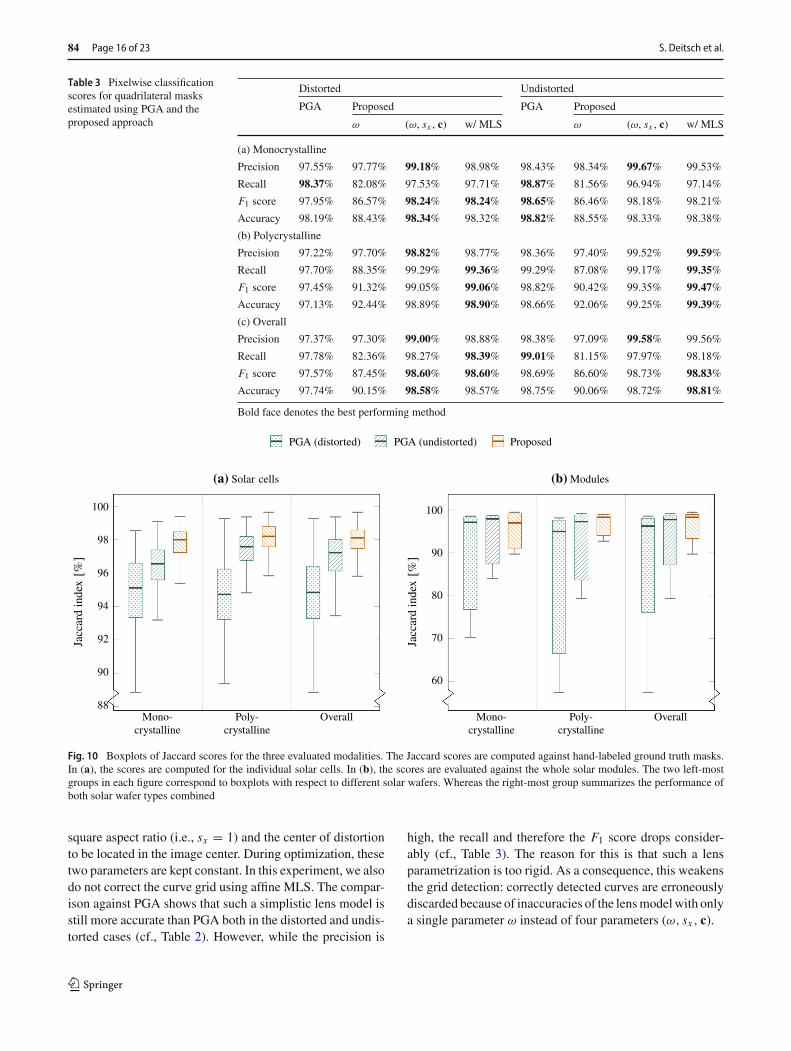
from the ground truth. The metric is provided for monocrys-talline and polycrystalline solar wafers separately, and forboth types combined. In all cases, the proposed approach out-performs both PGAvariants.We particularly notice that PGAgreatly benefits from lens distortion estimation. This under-lines our observation that the latter is essential for highlyaccurate segmentation.Pixelwise Classification Pixelwise scores for the simplifiedmasks of both methods are given in Table 3. For monocrys-talline PV modules, PGA generally achieves higher scores.However, highest scores are achieved only for images forwhich the lens distortion has been removed. The proposedmethod fails to segment a row of cells in a solar mod-ule resulting in a lower recall. However, for polycrystallinePV modules, the proposed method consistently outperformsPGA. In the overall score, the proposed method also out-performs the best-case evaluation for PGA on undistortedimages. However, PGA has highest recall, which is due tothe lower number of parameters of PGA.Weighted Jaccard Index The Jaccard scores summarizedas boxplots in Fig. 10 support the pixelwise classificationscores, showing that the proposed method is more accuratethan PGA. The latter, however, is slightly more robust. Forcomplete modules, the considerable spread of PGA is par-tially attributed to one major outlier. Overall, the proposedsegmentation pipeline is highly accurate. Particularly oncea cell is detected, the cell outline is accurately and robustlysegmented.
4.3.2 Ablation study
We ablate the lens distortion parameters and the post hocapplication of affine MLS to investigate their effect on theaccuracy and the success rate of the segmentation process.The ablation is performed both on original (i.e., distorted)EL images and undistorted ones.Distorted vs. Undistorted EL Images For the ablation study,we consider two main cases. In the undistorted case, bothreference and predicted masks are unwarped using estimatedlens distortion parameters. Then, quadrilaterals are fitted toindividual cell masks to allow a comparison against PGAwhich always yields such quadrilateral cell masks. For a faircomparison, PGA is also applied to undistorted images.
In the distorted case, however, the comparison is per-formed in the original image space. Since the proposedmethod yields a curved grid after applying the inverse oflens distortion,we synthesize a regular grid frombackwarpedcell masks. Specifically, we extract the contours of estimatedsolar cell masks to obtain the coordinates of the quadri-lateral in the unwarped image, and then apply the inverseof estimated geometric transformations to rectangle coordi-nates. Afterwards, we fit lines to each side of the backwarpedquadrilaterals along grid rows and columns. From their inter-sectionswe finally obtain the corner coordinates of each solarcells in the distorted image which we can use for comparisonagainst distorted PGA results.Parameterization First, we reduce the lens distortion modelto a single radial distortion parameter ω and assume both
123
84 Page 16 of 23 S. Deitsch et al.
Table 3 Pixelwise classificationscores for quadrilateral masksestimated using PGA and theproposed approach
Distorted Undistorted
PGA Proposed PGA Proposed
ω (ω, sx , c) w/ MLS ω (ω, sx , c) w/ MLS
(a) Monocrystalline
Precision 97.55% 97.77% 99.18% 98.98% 98.43% 98.34% 99.67% 99.53%
Recall 98.37% 82.08% 97.53% 97.71% 98.87% 81.56% 96.94% 97.14%
F1 score 97.95% 86.57% 98.24% 98.24% 98.65% 86.46% 98.18% 98.21%
Accuracy 98.19% 88.43% 98.34% 98.32% 98.82% 88.55% 98.33% 98.38%
(b) Polycrystalline
Precision 97.22% 97.70% 98.82% 98.77% 98.36% 97.40% 99.52% 99.59%
Recall 97.70% 88.35% 99.29% 99.36% 99.29% 87.08% 99.17% 99.35%
F1 score 97.45% 91.32% 99.05% 99.06% 98.82% 90.42% 99.35% 99.47%
Accuracy 97.13% 92.44% 98.89% 98.90% 98.66% 92.06% 99.25% 99.39%
(c) Overall
Precision 97.37% 97.30% 99.00% 98.88% 98.38% 97.09% 99.58% 99.56%
Recall 97.78% 82.36% 98.27% 98.39% 99.01% 81.15% 97.97% 98.18%
F1 score 97.57% 87.45% 98.60% 98.60% 98.69% 86.60% 98.73% 98.83%
Accuracy 97.74% 90.15% 98.58% 98.57% 98.75% 90.06% 98.72% 98.81%
Bold face denotes the best performing method
Mono-crystalline
Poly-crystalline
Overall88
90
92
94
96
98
100
Jaccardindex� %
�
(a) Solar cells
Mono-crystalline
Poly-crystalline
Overall
60
70
80
90
100
Jaccardindex� %
�
(b)Modules
PGA (distorted) PGA (undistorted) Proposed
Fig. 10 Boxplots of Jaccard scores for the three evaluated modalities. The Jaccard scores are computed against hand-labeled ground truth masks.In (a), the scores are computed for the individual solar cells. In (b), the scores are evaluated against the whole solar modules. The two left-mostgroups in each figure correspond to boxplots with respect to different solar wafers. Whereas the right-most group summarizes the performance ofboth solar wafer types combined
square aspect ratio (i.e., sx = 1) and the center of distortionto be located in the image center. During optimization, thesetwo parameters are kept constant. In this experiment, we alsodo not correct the curve grid using affine MLS. The compar-ison against PGA shows that such a simplistic lens model isstill more accurate than PGA both in the distorted and undis-torted cases (cf., Table 2). However, while the precision is
high, the recall and therefore the F1 score drops consider-ably (cf., Table 3). The reason for this is that such a lensparametrization is too rigid. As a consequence, this weakensthe grid detection: correctly detected curves are erroneouslydiscarded because of inaccuracies of the lensmodelwith onlya single parameter ω instead of four parameters (ω, sx , c).
123
Segmentation of photovoltaic module cells in uncalibrated electroluminescence... Page 17 of 23 84
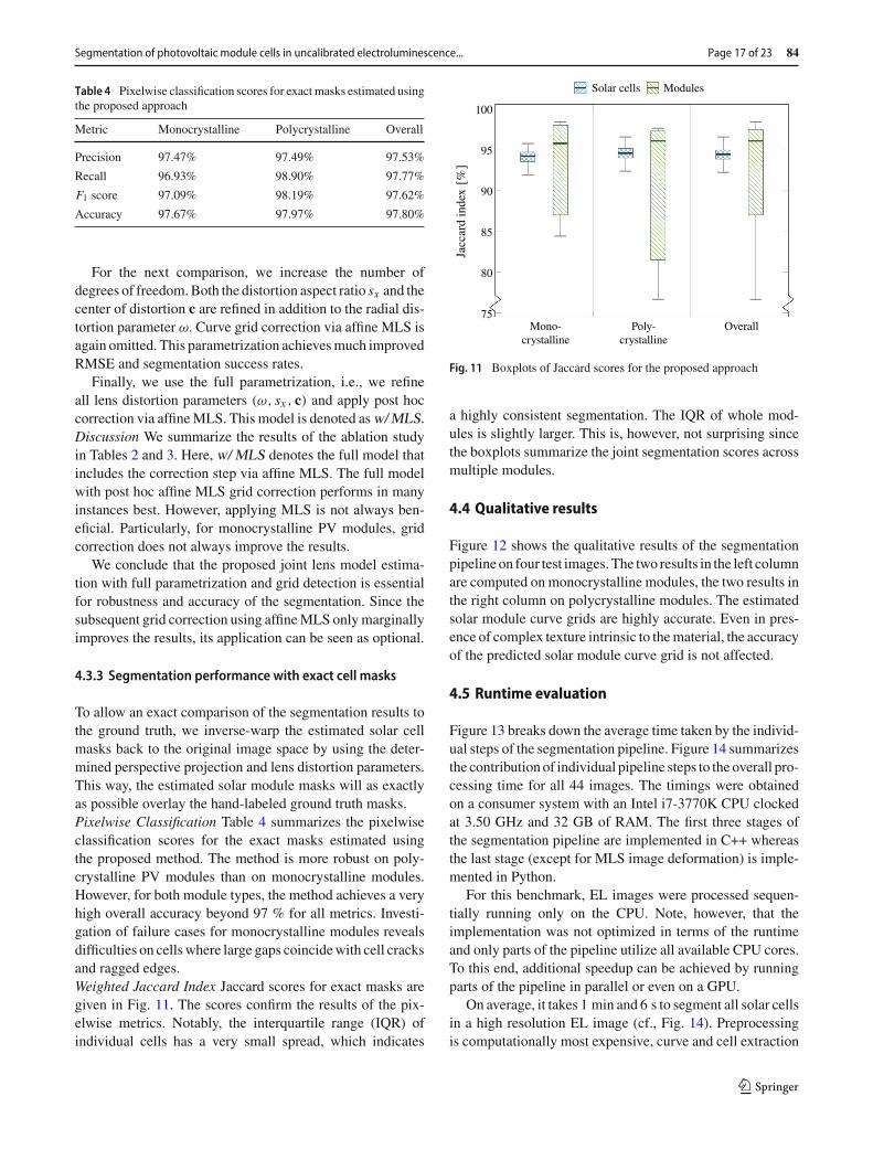
Table 4 Pixelwise classification scores for exact masks estimated usingthe proposed approach
Metric Monocrystalline Polycrystalline Overall
Precision 97.47% 97.49% 97.53%
Recall 96.93% 98.90% 97.77%
F1 score 97.09% 98.19% 97.62%
Accuracy 97.67% 97.97% 97.80%
For the next comparison, we increase the number ofdegrees of freedom.Both the distortion aspect ratio sx and thecenter of distortion c are refined in addition to the radial dis-tortion parameter ω. Curve grid correction via affine MLS isagain omitted. This parametrization achievesmuch improvedRMSE and segmentation success rates.
Finally, we use the full parametrization, i.e., we refineall lens distortion parameters (ω, sx , c) and apply post hoccorrection via affineMLS. This model is denoted as w/MLS.Discussion We summarize the results of the ablation studyin Tables 2 and 3. Here, w/ MLS denotes the full model thatincludes the correction step via affine MLS. The full modelwith post hoc affine MLS grid correction performs in manyinstances best. However, applying MLS is not always ben-eficial. Particularly, for monocrystalline PV modules, gridcorrection does not always improve the results.
We conclude that the proposed joint lens model estima-tion with full parametrization and grid detection is essentialfor robustness and accuracy of the segmentation. Since thesubsequent grid correction using affineMLS onlymarginallyimproves the results, its application can be seen as optional.
4.3.3 Segmentation performance with exact cell masks
To allow an exact comparison of the segmentation results tothe ground truth, we inverse-warp the estimated solar cellmasks back to the original image space by using the deter-mined perspective projection and lens distortion parameters.This way, the estimated solar module masks will as exactlyas possible overlay the hand-labeled ground truth masks.Pixelwise Classification Table 4 summarizes the pixelwiseclassification scores for the exact masks estimated usingthe proposed method. The method is more robust on poly-crystalline PV modules than on monocrystalline modules.However, for both module types, the method achieves a veryhigh overall accuracy beyond 97 % for all metrics. Investi-gation of failure cases for monocrystalline modules revealsdifficulties on cellswhere large gaps coincidewith cell cracksand ragged edges.Weighted Jaccard Index Jaccard scores for exact masks aregiven in Fig. 11. The scores confirm the results of the pix-elwise metrics. Notably, the interquartile range (IQR) ofindividual cells has a very small spread, which indicates
Mono-crystalline
Poly-crystalline
Overall75
80
85
90
95
100
Jaccardindex� %
�
Solar cells Modules
Fig. 11 Boxplots of Jaccard scores for the proposed approach
a highly consistent segmentation. The IQR of whole mod-ules is slightly larger. This is, however, not surprising sincethe boxplots summarize the joint segmentation scores acrossmultiple modules.
4.4 Qualitative results
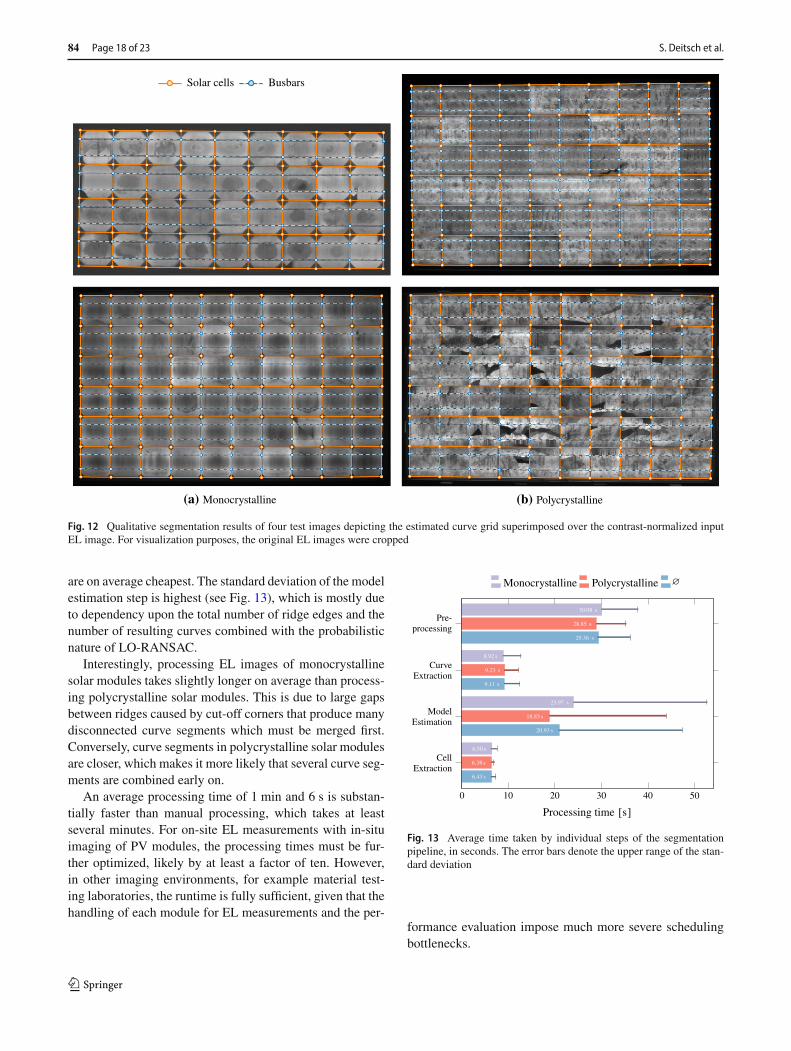
Figure 12 shows the qualitative results of the segmentationpipeline on four test images.The two results in the left columnare computed on monocrystalline modules, the two results inthe right column on polycrystalline modules. The estimatedsolar module curve grids are highly accurate. Even in pres-ence of complex texture intrinsic to thematerial, the accuracyof the predicted solar module curve grid is not affected.
4.5 Runtime evaluation
Figure 13 breaks down the average time taken by the individ-ual steps of the segmentation pipeline. Figure 14 summarizesthe contribution of individual pipeline steps to the overall pro-cessing time for all 44 images. The timings were obtainedon a consumer system with an Intel i7-3770K CPU clockedat 3.50 GHz and 32 GB of RAM. The first three stages ofthe segmentation pipeline are implemented in C++ whereasthe last stage (except for MLS image deformation) is imple-mented in Python.
For this benchmark, EL images were processed sequen-tially running only on the CPU. Note, however, that theimplementation was not optimized in terms of the runtimeand only parts of the pipeline utilize all available CPU cores.To this end, additional speedup can be achieved by runningparts of the pipeline in parallel or even on a GPU.
On average, it takes 1 min and 6 s to segment all solar cellsin a high resolution EL image (cf., Fig. 14). Preprocessingis computationally most expensive, curve and cell extraction
123
84 Page 18 of 23 S. Deitsch et al.
(a) Monocrystalline (b) Polycrystalline
Solar cells Busbars
Fig. 12 Qualitative segmentation results of four test images depicting the estimated curve grid superimposed over the contrast-normalized inputEL image. For visualization purposes, the original EL images were cropped
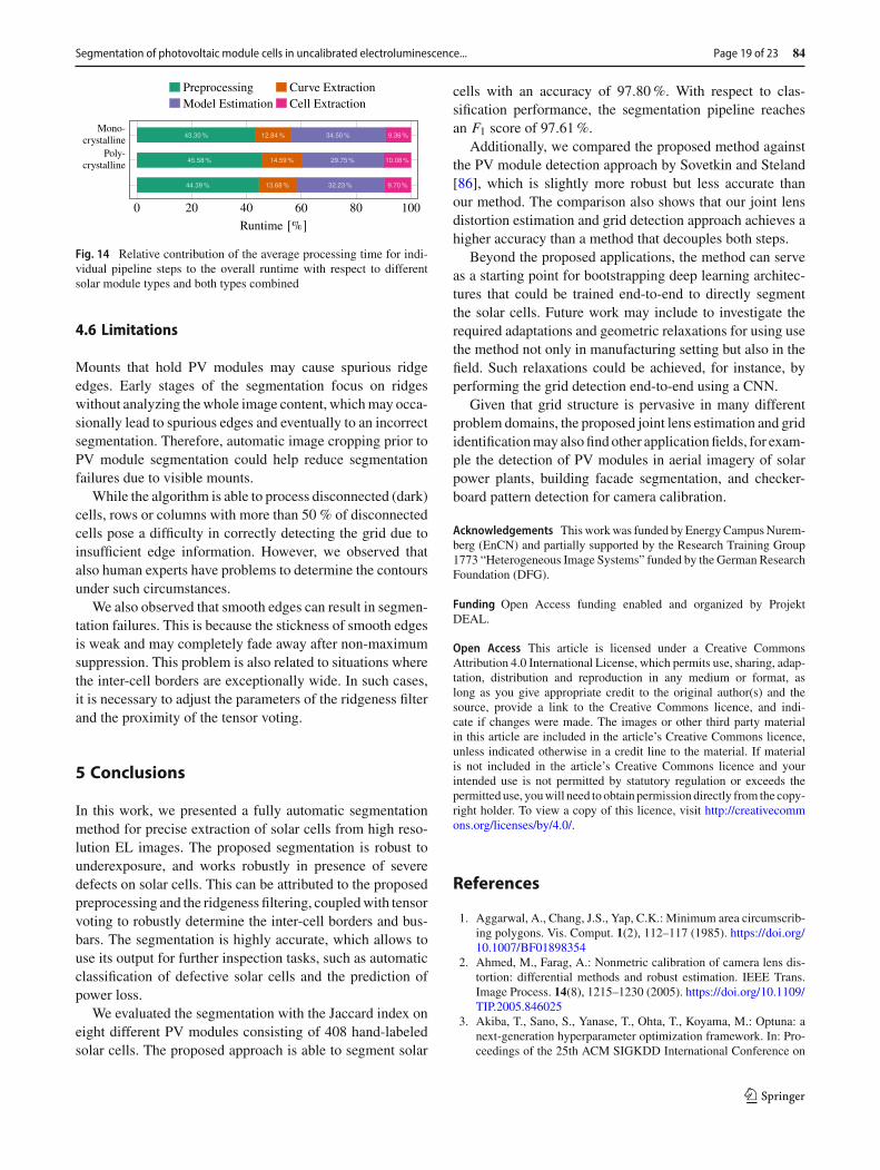
are on average cheapest. The standard deviation of the modelestimation step is highest (see Fig. 13), which is mostly dueto dependency upon the total number of ridge edges and thenumber of resulting curves combined with the probabilisticnature of LO-RANSAC.
Interestingly, processing EL images of monocrystallinesolar modules takes slightly longer on average than process-ing polycrystalline solar modules. This is due to large gapsbetween ridges caused by cut-off corners that produce manydisconnected curve segments which must be merged first.Conversely, curve segments in polycrystalline solar modulesare closer, which makes it more likely that several curve seg-ments are combined early on.
An average processing time of 1 min and 6 s is substan-tially faster than manual processing, which takes at leastseveral minutes. For on-site EL measurements with in-situimaging of PV modules, the processing times must be fur-ther optimized, likely by at least a factor of ten. However,in other imaging environments, for example material test-ing laboratories, the runtime is fully sufficient, given that thehandling of each module for EL measurements and the per-
0 10 20 30 40 50
Pre-processing
CurveExtraction
ModelEstimation
CellExtraction
30.08 s
8.92 s
23.97 s
6.50 s
28.85 s
9.23 s
18.83 s
6.38 s
29.36 s
9.11 s
20.93 s
6.43 s
Processing time �s�
Monocrystalline Polycrystalline
Fig. 13 Average time taken by individual steps of the segmentationpipeline, in seconds. The error bars denote the upper range of the stan-dard deviation
formance evaluation impose much more severe schedulingbottlenecks.
123
Segmentation of photovoltaic module cells in uncalibrated electroluminescence... Page 19 of 23 84
Fig. 14 Relative contribution of the average processing time for indi-vidual pipeline steps to the overall runtime with respect to differentsolar module types and both types combined
4.6 Limitations
Mounts that hold PV modules may cause spurious ridgeedges. Early stages of the segmentation focus on ridgeswithout analyzing thewhole image content, whichmay occa-sionally lead to spurious edges and eventually to an incorrectsegmentation. Therefore, automatic image cropping prior toPV module segmentation could help reduce segmentationfailures due to visible mounts.
While the algorithm is able to process disconnected (dark)cells, rows or columns with more than 50 % of disconnectedcells pose a difficulty in correctly detecting the grid due toinsufficient edge information. However, we observed thatalso human experts have problems to determine the contoursunder such circumstances.
We also observed that smooth edges can result in segmen-tation failures. This is because the stickness of smooth edgesis weak and may completely fade away after non-maximumsuppression. This problem is also related to situations wherethe inter-cell borders are exceptionally wide. In such cases,it is necessary to adjust the parameters of the ridgeness filterand the proximity of the tensor voting.
5 Conclusions
In this work, we presented a fully automatic segmentationmethod for precise extraction of solar cells from high reso-lution EL images. The proposed segmentation is robust tounderexposure, and works robustly in presence of severedefects on solar cells. This can be attributed to the proposedpreprocessing and the ridgeness filtering, coupledwith tensorvoting to robustly determine the inter-cell borders and bus-bars. The segmentation is highly accurate, which allows touse its output for further inspection tasks, such as automaticclassification of defective solar cells and the prediction ofpower loss.
We evaluated the segmentation with the Jaccard index oneight different PV modules consisting of 408 hand-labeledsolar cells. The proposed approach is able to segment solar
cells with an accuracy of 97.80%. With respect to clas-sification performance, the segmentation pipeline reachesan F1 score of 97.61%.
Additionally, we compared the proposed method againstthe PV module detection approach by Sovetkin and Steland[86], which is slightly more robust but less accurate thanour method. The comparison also shows that our joint lensdistortion estimation and grid detection approach achieves ahigher accuracy than a method that decouples both steps.
Beyond the proposed applications, the method can serveas a starting point for bootstrapping deep learning architec-tures that could be trained end-to-end to directly segmentthe solar cells. Future work may include to investigate therequired adaptations and geometric relaxations for using usethe method not only in manufacturing setting but also in thefield. Such relaxations could be achieved, for instance, byperforming the grid detection end-to-end using a CNN.
Given that grid structure is pervasive in many differentproblem domains, the proposed joint lens estimation and grididentificationmay alsofindother applicationfields, for exam-ple the detection of PV modules in aerial imagery of solarpower plants, building facade segmentation, and checker-board pattern detection for camera calibration.
Acknowledgements Thisworkwas funded byEnergyCampusNurem-berg (EnCN) and partially supported by the Research Training Group1773 “Heterogeneous Image Systems” funded by the German ResearchFoundation (DFG).
Funding Open Access funding enabled and organized by ProjektDEAL.
Open Access This article is licensed under a Creative CommonsAttribution 4.0 International License, which permits use, sharing, adap-tation, distribution and reproduction in any medium or format, aslong as you give appropriate credit to the original author(s) and thesource, provide a link to the Creative Commons licence, and indi-cate if changes were made. The images or other third party materialin this article are included in the article’s Creative Commons licence,unless indicated otherwise in a credit line to the material. If materialis not included in the article’s Creative Commons licence and yourintended use is not permitted by statutory regulation or exceeds thepermitted use, youwill need to obtain permission directly from the copy-right holder. To view a copy of this licence, visit http://creativecommons.org/licenses/by/4.0/.
References
1. Aggarwal, A., Chang, J.S., Yap, C.K.: Minimum area circumscrib-ing polygons. Vis. Comput. 1(2), 112–117 (1985). https://doi.org/10.1007/BF01898354
2. Ahmed, M., Farag, A.: Nonmetric calibration of camera lens dis-tortion: differential methods and robust estimation. IEEE Trans.Image Process. 14(8), 1215–1230 (2005). https://doi.org/10.1109/TIP.2005.846025
3. Akiba, T., Sano, S., Yanase, T., Ohta, T., Koyama, M.: Optuna: anext-generation hyperparameter optimization framework. In: Pro-ceedings of the 25th ACM SIGKDD International Conference on
123

84 Page 20 of 23 S. Deitsch et al.
Knowledge Discovery and Data Mining, Association for Comput-ing Machinery, New York, NY, USA, KDD ’19, pp. 2623–2631,(2019) https://doi.org/10.1145/3292500.3330701
4. Aloimonos, J.: Shape from texture. Biol. Cybern. 58(5), 345–360(1988). https://doi.org/10.1007/BF00363944
5. Anwar, S.A., Abdullah, M.Z.: Micro-crack detection of multicrys-talline solar cells featuring an improved anisotropic diffusion filterand image segmentation technique. EURASIP J. Image VideoProcess. 2014(1), 15 (2014). https://doi.org/10.1186/1687-5281-2014-15
6. Barber, C.B., Dobkin, D.P., Dobkin, D.P., Huhdanpaa, H.: Thequickhull algorithm for convex hulls. ACM Trans. Math. Softw.22(4), 469–483 (1996). https://doi.org/10.1145/235815.235821
7. Bergstra, J., Bengio, Y.: Random search for hyper-parameter opti-mization. J. Mach. Learn. Res. 13, 281–305 (2012)
8. Bergstra, J., Bardenet, R., Bengio, Y., Kégl, B.: Algorithms forhyper-parameter optimization. In: Shawe-Taylor, J., Zemel, R.,Bartlett, P., Pereira, F.,Weinberger, K.Q. (eds.) Advances in NeuralInformation Processing Systems, vol. 24, pp. 2546–2554. CurranAssociates, New York (2011)
9. Bergstra, J., Yamins, D., Cox, D.D.: Making a science of modelsearch: hyperparameter optimization in hundreds of dimensionsfor vision architectures. In: Proceedings of the 30th InternationalConference on International Conference on Machine Learning,ICML’13, pp. 115–123 (2013)
10. Breitenstein, O., Bauer, J., Bothe, K., Hinken, D., Müller, J.,Kwapil,W., Schubert,M.C.,Warta,W.: Can luminescence imagingreplace lock-in thermography on solar cells? IEEE J. Photovolt.1(2), 159–167 (2011). https://doi.org/10.1109/JPHOTOV.2011.2169394
11. Brown, D.C.: Close-range camera calibration. Photogramm. Eng.Remote Sens. 37, 855–866 (1971). https://doi.org/10.1.1.14.6358
12. Buerhop-Lutz, C., Deitsch, S., Maier, A., Gallwitz, F., Berger,S., Doll, B., Hauch, J., Camus, C., Brabec, C.J.: A benchmarkfor visual identification of defective solar cells in electrolumines-cence imagery. In: 35th European PV Solar Energy Conferenceand Exhibition, pp. 1287–1289 (2018) https://doi.org/10.4229/35thEUPVSEC20182018-5CV.3.15
13. Chenni, R., Makhlouf, M., Kerbache, T., Bouzid, A.: A detailedmodeling method for photovoltaic cells. Energy 32(9), 1724–1730(2007). https://doi.org/10.1016/j.energy.2006.12.006
14. Chierichetti, F., Kumar, R., Pandey, S., Vassilvitskii, S.: Findingthe Jaccard median. In: Symposium on Discrete Algorithms, pp.293–311, Austin, Texas (2010)
15. Chum, O., Matas, J., Kittler, J.: Locally optimized RANSAC. In:Michaelis, B., Krell, G. (eds.) Pattern Recognition, vol. 2781, pp.236–243. Springer, Berlin (2003). https://doi.org/10.1007/978-3-540-45243-0_31
16. Claus, D., Fitzgibbon,A.W.:A plumbline constraint for the rationalfunction lens distortion model. In: British Machine Vision Confer-ence (BMVC), pp. 99–108 (2005) https://doi.org/10.5244/C.19.10
17. Claus, D., Fitzgibbon, A.W.: A rational function lens distortionmodel for general cameras. Conf. Comput. Vis. Pattern Recognit.(CVPR) 1, 213–219 (2005b). https://doi.org/10.1109/CVPR.2005.43
18. Deitsch, S., Christlein, V., Berger, S., Buerhop-Lutz, C., Maier, A.,Gallwitz, F., Riess, C.: Automatic classification of defective pho-tovoltaic module cells in electroluminescence images. Sol. Energy185, 455–468 (2019). https://doi.org/10.1016/j.solener.2019.02.067. (arXiv:1807.02894)
19. Devernay, F.: A non-maxima suppression method for edge detec-tion with sub-pixel accuracy. Technical Report, RR-2724, INRIA(1995) https://hal.inria.fr/inria-00073970
20. Devernay, F., Faugeras, O.: Straight lines have to be straight.Mach. Vis. Appl. 13(1), 14–24 (2001). https://doi.org/10.1007/PL00013269
21. Douglas, D.H., Peucker, T.K.: Algorithms for the reduction of thenumber of points required to represent a digitized line or its cari-cature. Cartogr. Int. J. Geogr. Inf. Geovis. 10(2), 112–122 (1973).https://doi.org/10.3138/fm57-6770-u75u-7727
22. Ester, M., Kriegel, H.P., Sander, J., Xu, X.: A density-based algo-rithm for discovering clusters in large spatial databases with noise.In: Proceedings of the 2nd International Conference on Knowl-edgeDiscovery andDataMining,AAAIPress, Portland,OR,USA,KDD’96, pp 226–231 (1996)
23. Fabijanska, A.: A survey of subpixel edge detection methods forimages of heat-emitting metal specimens. Int. J. Appl. Math. Com-put. Sci. 22(3), 695–710 (2012). https://doi.org/10.2478/v10006-012-0052-3
24. Fischler, M.A., Bolles, R.C.: Random sample consensus: aparadigm for model fitting with applications to image analysis andautomated cartography. Commun. ACM 24(6), 381–395 (1981).https://doi.org/10.1145/358669.358692
25. Fitzgibbon, A.: Simultaneous linear estimation of multiple viewgeometry and lens distortion. IEEE Comput. Soc. Conf. Comput.Vis. Pattern Recognit. 1, 125–132 (2001). https://doi.org/10.1109/CVPR.2001.990465
26. Flocke,N.:Algorithm954: an accurate and efficient cubic andquar-tic equation solver for physical applications. ACM Trans. Math.Softw. 41(4), 30:1-30:24 (2015). https://doi.org/10.1145/2699468
27. Franken, E., van Almsick, M., Rongen, P., Florack, L., terHaar Romeny, B.: An efficient method for tensor voting usingsteerable filters. In: Leonardis,A., Bischof,H., Pinz,A. (eds.) Euro-peanConference onComputerVision (ECCV), pp. 228–240 (2006)https://doi.org/10.1007/11744085_18
28. Franken, E., Rongen, P., van Almsick, M., ter Haar Romeny,B.: Detection of electrophysiology catheters in noisy fluoroscopyimages. In: Larsen, R., Nielsen, M., Sporring, J. (eds.) MedicalImageComputing andComputer-Assisted Intervention—MICCAI2006, Springer, Berlin, Heidelberg, pp. 25–32 (2006) https://doi.org/10.1007/11866763_4
29. Fürsattel, P., Dotenco, S., Placht, S., Balda, M., Maier, A., Riess,C.: OCPAD—occluded checkerboard pattern detector. In: WinterConference on Applications of Computer Vision (WACV), IEEE,(2016) https://doi.org/10.1109/WACV.2016.7477565
30. Grompone von Gioi, R., Randall, G.: A sub-pixel edge detector: animplementation of the Canny/Devernay algorithm. Image Process.On Line 7, 347–372 (2017). https://doi.org/10.5201/ipol.2017.216
31. Girshick, R.B.: Fast R-CNN. In: IEEE International Conference onComputer Vision, pp. 1440–1448 (2015), https://doi.org/10.1109/ICCV.2015.169
32. Girshick, R.B.,Donahue, J., Darrell, T.,Malik, J.: Rich feature hier-archies for accurate object detection and semantic segmentation.In: IEEEConference on Computer Vision and Pattern Recognition,pp. 580–587 (2014). https://doi.org/10.1109/CVPR.2014.81
33. Golub, G.H., Van Loan, C.F.: Matrix Computations, 4th edn. JohnsHopkins Studies in theMathematical Sciences, JohnsHopkinsUni-versity Press (2013)
34. Gonzalez, R.C., Woods, R.E.: Digital Image Processing, 4th edn.Pearson, New York (2018)
35. Goodfellow, I., Bengio, Y., Courville, A.: Deep Learning. MITPress, Cambridge (2016)
36. Ha, H., Perdoch, M., Alismail, H., Kweon, I.S., Sheikh, Y.: Deltillegrids for geometric camera calibration. In: International Confer-ence on Computer Vision (ICCV), pp. 5354–5362 (2017). https://doi.org/10.1109/ICCV.2017.571
37. Harker, M., O’Leary, P., Zsombor-Murray, P.: Direct type-specificconic fitting and eigenvalue bias correction. Image Vis. Comput.26(3), 372–381 (2008). https://doi.org/10.1016/j.imavis.2006.12.006
38. Hartley, R., Zisserman, A.: Multiple View Geometry in ComputerVision, 2nd edn. Cambridge University Press, New York (2004)
123

Segmentation of photovoltaic module cells in uncalibrated electroluminescence... Page 21 of 23 84
39. He, K., Gkioxari, G., Dollár, P., Girshick, R.B.: Mask R-CNN.In: IEEE International Conference on Computer Vision, pp. 2980–2988 (2017). https://doi.org/10.1109/ICCV.2017.322
40. He, X., Zemel, R.S., Carreira-Perpinan, M.A.: Multiscale con-ditional random fields for image labeling. IEEE Conf. Comput.Vis. Pattern Recognit. 2, 695–702 (2004). https://doi.org/10.1109/CVPR.2004.1315232
41. Hoffmann, M., Ernst, A., Bergen, T., Hettenkofer, S., Garbas, J.U.:A robust chessboard detector for geometric camera calibration. In:International Joint Conference on Computer Vision, Imaging andComputer Graphics Theory and Applications (VISIGRAPP), pp.34–43 (2017). https://doi.org/10.5220/0006104300340043
42. IEC TS 60904-13:2018 (2018) Photovoltaic devices—part 13:Electroluminescence of photovoltaic modules. Technical specifi-cation, International Electrotechnical Commission
43. Ioffe, S.: Improved consistent sampling, weighted minhash and L1
sketching. In: International Conference on Data Mining, pp. 246–255 (2010). https://doi.org/10.1109/ICDM.2010.80
44. Jaderberg, M., Simonyan, K., Zisserman, A., Kavukcuoglu, K.:Spatial transformer networks. In: Cortes, C., Lawrence, N.D., Lee,D.D., Sugiyama, M., Garnett, R. (eds.) Advances in Neural Infor-mation Processing Systems, 28, pp. 2017–2025. Curran AssociatesInc, New York (2015)
45. Jenkins, M.A., Traub, J.F.: A three-stage algorithm for real poly-nomials using quadratic iteration. J. Numer. Anal. 7(4), 545–566(1970). https://doi.org/10.1137/0707045
46. Karatepe, E., Boztepe, M., Çolak, M.: Development of a suitablemodel for characterizing photovoltaic arrays with shaded solarcells. Sol. Energy 81(8), 977–992 (2007). https://doi.org/10.1016/j.solener.2006.12.001
47. Kaushika, N.D., Gautam, N.K.: Energy yield simulations of inter-connected solar PV arrays. IEEE Trans. Energy Convers. 18(1),127–134 (2003). https://doi.org/10.1109/TEC.2002.805204
48. Kovesi, P.:MATLABandOctave functions for computer vision andimage processing (2017). http://www.peterkovesi.com/matlabfns
49. Kushner, H.J.: A new method of locating the maximum point of anarbitrary multipeak curve in the presence of noise. J. Basic Eng.86(1), 97–106 (1964). https://doi.org/10.1115/1.3653121
50. Levenberg, K.: A method for the solution of certain non-linearproblems in least squares. Q. Appl. Math. 2(2), 164–168 (1944)
51. Li, Y., Qi, H., Dai, J., Ji, X., Wei, Y.: Fully convolutional instance-aware semantic segmentation. In: IEEE Conference on ComputerVision and Pattern Recognition, pp. 4438–4446 (2017). https://doi.org/10.1109/CVPR.2017.472
52. Lin, C.H., Lucey, S.: Inverse compositional spatial transformernetworks. In: IEEE Conference on Computer Vision and PatternRecognition (CVPR), IEEE, pp. 2252–2260 (2017). https://doi.org/10.1109/CVPR.2017.242
53. Lindeberg, T.: Scale-space theory: a basic tool for analyzing struc-tures at different scales. J. Appl. Stat. 21(1–2), 225–270 (1994).https://doi.org/10.1080/757582976
54. Lindeberg, T.: Edge detection and ridge detection with automaticscale selection. In: Proceedings of the Conference on ComputerVision and Pattern Recognition, pp. 465–470 (1996). https://doi.org/10.1109/CVPR.1996.517113
55. Lindeberg, T.: Edge detection and ridge detection with automaticscale selection. Int. J. Comput. Vis. 30(2), 117–156 (1998). https://doi.org/10.1023/A:1008097225773
56. Long, J., Shelhamer, E., Darrell, T.: Fully convolutional networksfor semantic segmentation. In: Conference on Computer Visionand Pattern Recognition (CVPR), pp. 3431–3440 (2015). https://doi.org/10.1109/CVPR.2015.7298965
57. Marquardt,D.W.:An algorithm for least-squares estimation of non-linear parameters. J. Soc. Ind. Appl. Math. 11(2), 431–441 (1963).https://doi.org/10.1137/0111030
58. Masri, S.F., Bekey, G.A., Safford, F.B.: A global optimization algo-rithm using adaptive random search. Appl. Math. Comput. 7(4),353–375 (1980). https://doi.org/10.1016/0096-3003(80)90027-2
59. Mauk, M.G.: Image processing for solar cell analysis, diagnosticsand quality assurance inspection. In: Image Processing: Concepts,Methodologies, Tools, and Applications, IGI Global, chap 71, pp.1426–1462 (2013)
60. Mayr, M., Hoffmann, M., Maier, A., Christlein, V.: Weakly super-vised segmentation of cracks on solar cells using normalized L pnorm. In: 2019 IEEE International Conference on Image Process-ing (ICIP), pp. 1885–1889 (2019). https://doi.org/10.1109/ICIP.2019.8803116
61. Medioni, G., Tang, C.K., Lee, M.S.: Tensor voting: theory andapplications. In: Proceedings of RFIA (2000)
62. Mehta, S., Azad, A.P., Chemmengath, S.A., Raykar, V., Kalya-naraman, S.: DeepSolarEye: power loss prediction and weaklysupervised soiling localization via fully convolutional networksfor solar panels. In: Winter Conference on Applications of Com-puter Vision (WACV), pp. 333–342 (2018). https://doi.org/10.1109/WACV.2018.00043
63. Mockus, J.: On Bayesian methods for seeking the extremum. In:Marchuk, G.I. (ed.) IFIP Technical Conference on OptimizationTechniques, pp. 400–404. Springer, Berlin (1975)
64. Myronenko, A., Song, X.: Point set registration: coherent pointdrift. IEEE Trans. Pattern Anal. Mach. Intell. 32(12), 2262–2275(2010). https://doi.org/10.1109/TPAMI.2010.46
65. Nian, B., Fu, Z., Wang, L., Cao, X.: Automatic detection ofdefects in solar modules: image processing in detecting. In: 2010International Conference on Computational Intelligence and Soft-ware Engineering, IEEE, pp. 1–4 (2010), https://doi.org/10.1109/WICOM.2010.5600703
66. Nocedal, J., Wright, S.J.: Numerical Optimization, OperationsResearch and Financial Engineering, vol. 43, 2nd edn. Springer,New York (2006). https://doi.org/10.1007/978-0-387-40065-5
67. Otsu, N.: A threshold selectionmethod fromgray-level histograms.IEEETrans. Syst.ManCybern. 9(1), 62–66 (1979). https://doi.org/10.1109/TSMC.1979.4310076
68. Pitas, I.: Digital Image Processing Algorithms. Prentice-Hall Inc,Upper Saddle River (1993)
69. Placht, S., Fürsattel, P., Mengue, E.A., Hofmann, H., Schaller,C., Balda, M., Angelopoulou, E.: ROCHADE: robust checker-board advanced detection for camera calibration. In: Fleet, D.,Pajdla, T., Schiele, B., Tuytelaars, T. (eds.) European Conferenceon Computer Vision (ECCV), Lecture Notes in Computer Sci-ence, vol. 8692, pp. 766–779 (2014). https://doi.org/10.1007/978-3-319-10593-2_50
70. Potthoff, T., Bothe, K., Eitner, U., Hinken, D., Köntges, M.:Detection of the voltage distribution in photovoltaic modules byelectroluminescence imaging. Prog. Photovolt. Res. Appl. 18(2),100–106 (2010). https://doi.org/10.1002/pip.941
71. Prasad, D.K., Leung, M.K.H., Quek, C., Cho, S.Y.: A novelframework for making dominant point detection methods non-parametric. Image Vis. Comput. 30(11), 843–859 (2012). https://doi.org/10.1016/j.imavis.2012.06.010
72. Quaschning, V., Hanitsch, R.: Numerical simulation of current-voltage characteristics of photovoltaic systems with shaded solarcells. Sol. Energy 56(6), 513–520 (1996). https://doi.org/10.1016/0038-092X(96)00006-0
73. Ramer, U.: An iterative procedure for the polygonal approximationof plane curves. Comput. Graph. Image Process. 1(3), 244–256(1972). https://doi.org/10.1016/S0146-664X(72)80017-0
74. Rastrigin, L.A.: The convergence of the random search method inthe extremal control of a many parameter system. Autom. RemoteControl 24, 1337–1342 (1963)
75. Ren, S., He, K., Girshick, R., Sun, J.: Faster R-CNN: towards real-time object detection with region proposal networks. IEEE Trans.
123

84 Page 22 of 23 S. Deitsch et al.
Pattern Anal. Mach. Intell. 39(6), 1137–1149 (2017). https://doi.org/10.1109/TPAMI.2016.2577031
76. van Rijsbergen, C.J.: Information Retrieval, 2nd edn. Butterworth-Heinemann, Oxford (1979)
77. Ronneberger, O., Fischer, P., Brox, T.: U-Net: convolutional net-works for biomedical image segmentation. In: Navab, N., Horneg-ger, J., Wells, W.M., Frangi, A.F. (eds.) Medical Image Computingand Computer-Assisted Intervention—MICCAI 2015, pp. 234–241. Springer, Cham (2015). https://doi.org/10.1007/978-3-319-24574-4_28
78. Rosten, E., Loveland, R.: Camera distortion self-calibration usingthe plumb-line constraint and minimal Hough entropy. Mach. Vis.Appl. 22(1), 77–85 (2011). https://doi.org/10.1007/s00138-009-0196-9. (arXiv:0810.4426)
79. Rufli, M., Scaramuzza, D., Siegwart, R.: Automatic detection ofcheckerboards on blurred and distorted images. In: InternationalConference on Intelligent Robots and Systems, pp. 3121–3126(2008). https://doi.org/10.1109/IROS.2008.4650703
80. Saeed, K., Tabedzki, M., Rybnik, M., Adamski, M.: K3M: a uni-versal algorithm for image skeletonization and a review of thinningtechniques. Int. J.Appl.Math.Comput. Sci.20(2), 317–335 (2010).https://doi.org/10.2478/v10006-010-0024-4
81. Schaefer, S., McPhail, T., Warren, J.: Image deformation usingmoving least squares. ACM Trans. Graph. 25(3), 533 (2006).https://doi.org/10.1145/1141911.1141920
82. Schrack, G., Choit, M.: Optimized relative step size randomsearches. Math. Program. 10(1), 230–244 (1976). https://doi.org/10.1007/BF01580669
83. Schumer,M., Steiglitz, K.: Adaptive step size random search. IEEETrans. Autom. Control 13(3), 270–276 (1968). https://doi.org/10.1109/TAC.1968.1098903
84. Snoek, J., Larochelle, H., Adams, R.P.: Practical Bayesian opti-mization of machine learning algorithms. In: Pereira, F., Burges,C.J.C., Bottou, L., Weinberger, K.Q. (eds.) Advances in NeuralInformation Processing Systems, vol. 25, pp. 2951–2959. CurranAssociates Inc, New York (2012)
85. Solis, F.J., Wets, R.J.B.: Minimization by random search tech-niques. Math. Oper. Res. 6(1), 19–30 (1981). https://doi.org/10.1287/moor.6.1.19
86. Sovetkin, E., Steland, A.: Automatic processing and solar celldetection in photovoltaic electroluminescence images. Integr.Comput. Aided Eng. 26(2), 123–137 (2019). https://doi.org/10.3233/ICA-180588
87. Spataru, S., Hacke, P., Sera, D.: Automatic detection and evalua-tion of solar cell micro-cracks in electroluminescence images usingmatched filters. In: 2016 IEEE 43rd Photovoltaic Specialists Con-ference (PVSC), pp. 1602–1607 (2016). https://doi.org/10.1109/PVSC.2016.7749891
88. Spertino, F., Ciocia, A., Leo, P.D., Tommasini, R., Berardone, I.,Corrado, M., Infuso, A., Paggi, M.: A power and energy procedurein operating photovoltaic systems to quantify the losses accordingto the causes. Sol. Energy 118, 313–326 (2015). https://doi.org/10.1016/j.solener.2015.05.033
89. Stromer, D., Vetter, A., Oezkan, H.C., Probst, C., Maier, A.:Enhanced crack segmentation (eCS): a reference algorithm for seg-menting cracks in multicrystalline silicon solar cells. IEEE J. Pho-tovolt. 9(3), 752–758 (2019). https://doi.org/10.1109/JPHOTOV.2019.2895808
90. Tsai, D.M., Wu, S.C., Li, W.C.: Defect detection of solar cells inelectroluminescence images using Fourier image reconstruction.Sol. Energy Mater. Sol. Cells 99, 250–262 (2012). https://doi.org/10.1016/j.solmat.2011.12.007
91. Tsai,D.M.,Wu, S.C., Chiu,W.Y.:Defect detection in solarmodulesusing ICA basis images. IEEE Trans. Ind. Inform. 9(1), 122–131(2013). https://doi.org/10.1109/TII.2012.2209663
92. Tsai, R.Y.: A versatile camera calibration technique for high-accuracy 3D machine vision metrology using off-the-shelf TVcameras and lenses. IEEE J. Robot. Autom. 3(4), 323–344 (1987).https://doi.org/10.1109/JRA.1987.1087109
93. Tseng, D.C., Liu, Y.S., Chou, C.M.: Automatic finger interrup-tion detection in electroluminescence images of multicrystallinesolar cells. Math. Probl. Eng. 2015, 1–12 (2015). https://doi.org/10.1155/2015/879675
Publisher’s Note Springer Nature remains neutral with regard to juris-dictional claims in published maps and institutional affiliations.
Sergiu Deitsch received a masters degree in computer science fromNuremberg Institute of Technology in 2011. He is currently pursuinga Ph.D. degree with the Pattern Recognition Lab at the Friedrich-Alexander University Erlangen-Nürnberg. His research interestsinclude various aspects of image processing, object detection and track-ing, sensor fusion, and machine learning.
Claudia Buerhop-Lutz has been working as a scientist in the field ofquality control of photovoltaics for more than 15 years. She is spe-cialized in using imaging techniques, such as electroluminescence andthermography, for defect detection in solar modules.
Evgenii Sovetkin graduated in mathematics in 2013 and received hisPh.D. degree at RWTH University Aachen in 2020. From 2019, heis working in IEK-5, Institute of Photovoltaics at ForschungszentrumJülich. His research interests include statistical modeling for high-dimensional data analysis and statistical modeling for physics.
Ansgar Steland received M.Sc. and Ph.D. degrees in mathematicsfrom the Georg-August University of Göttingen, Germany. He heldpositions as an assistant at the Technical University of Berlin, Berlin,Germany, as a consultant in industry, as a postdoc at the EuropeanUniversity Viadrina of Frankfurt/Oder, Germany, and as a lecturer atthe Faculty of Mathematics at the Ruhr-University Bochum. Since2006, he is Full Professor at RWTH Aachen University, Germany,where he holds the Chair of Stochastics at the Institute of Statis-tics. He is an Elected Member of the International Statistical Insti-tute (ISI), acts as the speaker of the Society for Reliability, Qualityand Safety, and chairs the Section on Statistics in Natural Sciencesand Technology of the German Statistical Society (DStatG). He orga-nized and co-organized several international workshops and invitedsessions, edited several proceedings and special journal issues, andserves the community as associate editor. His current research interestsare in nonparametric statistics and high-dimensional inference, statis-tical and machine learning, neural networks, change-point detectionand sequential analysis, image processing, and applications in photo-voltaics, quality control and econometrics.
123
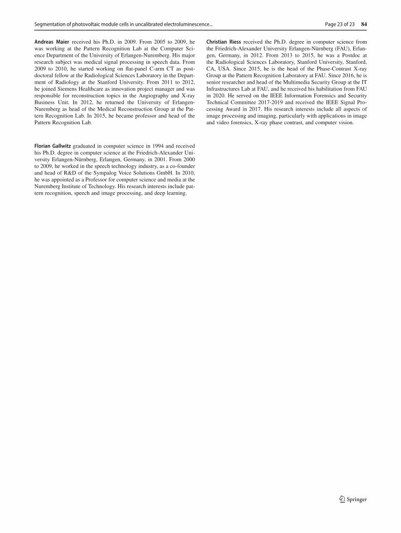
Segmentation of photovoltaic module cells in uncalibrated electroluminescence... Page 23 of 23 84
Andreas Maier received his Ph.D. in 2009. From 2005 to 2009, hewas working at the Pattern Recognition Lab at the Computer Sci-ence Department of the University of Erlangen-Nuremberg. His majorresearch subject was medical signal processing in speech data. From2009 to 2010, he started working on flat-panel C-arm CT as post-doctoral fellow at the Radiological Sciences Laboratory in the Depart-ment of Radiology at the Stanford University. From 2011 to 2012,he joined Siemens Healthcare as innovation project manager and wasresponsible for reconstruction topics in the Angiography and X-rayBusiness Unit. In 2012, he returned the University of Erlangen-Nuremberg as head of the Medical Reconstruction Group at the Pat-tern Recognition Lab. In 2015, he became professor and head of thePattern Recognition Lab.
Florian Gallwitz graduated in computer science in 1994 and receivedhis Ph.D. degree in computer science at the Friedrich-Alexander Uni-versity Erlangen-Nürnberg, Erlangen, Germany, in 2001. From 2000to 2009, he worked in the speech technology industry, as a co-founderand head of R&D of the Sympalog Voice Solutions GmbH. In 2010,he was appointed as a Professor for computer science and media at theNuremberg Institute of Technology. His research interests include pat-tern recognition, speech and image processing, and deep learning.
Christian Riess received the Ph.D. degree in computer science fromthe Friedrich-Alexander University Erlangen-Nürnberg (FAU), Erlan-gen, Germany, in 2012. From 2013 to 2015, he was a Postdoc atthe Radiological Sciences Laboratory, Stanford University, Stanford,CA, USA. Since 2015, he is the head of the Phase-Contrast X-rayGroup at the Pattern Recognition Laboratory at FAU. Since 2016, he issenior researcher and head of the Multimedia Security Group at the ITInfrastructures Lab at FAU, and he received his habilitation from FAUin 2020. He served on the IEEE Information Forensics and SecurityTechnical Committee 2017-2019 and received the IEEE Signal Pro-cessing Award in 2017. His research interests include all aspects ofimage processing and imaging, particularly with applications in imageand video forensics, X-ray phase contrast, and computer vision.
123


![Uncalibrated 3D Stereo Image-based Dynamic Visual Servoing ... · uncalibrated visual servoing with robot dynamics has been tackled with new adaptive controllers [11],[26]. However,](https://img.pdfslide.us/doc/110x75/606d9bc0175fff2c42161cce/uncalibrated-3d-stereo-image-based-dynamic-visual-servoing-uncalibrated-visual.jpg)


![Enforcing Consistency Constraints in Uncalibrated Multiple ...wojtek/papers/multiHomogr.pdf · Enforcing Consistency Constraints in Uncalibrated Multiple ... tection [25, 46] or enhanced](https://img.pdfslide.us/doc/110x75/5f0d905a7e708231d43afb29/enforcing-consistency-constraints-in-uncalibrated-multiple-wojtekpapersmultihomogrpdf.jpg)


![Uncalibrated pulse contour derived stroke volume variation predicts[1]](https://img.pdfslide.us/doc/110x75/556b02c5d8b42a2a4f8b514c/uncalibrated-pulse-contour-derived-stroke-volume-variation-predicts1.jpg)