Final Review

• Final will cover all lectures, book, and class assignments.

• New lectures since last test are 18 – 26, summarized here. Over half the test will come from this last portion of the course.

Lecture 18

• Review the following satellite products:

• Landsat MSS

• Landsat TM

• SPOT

• IKONOS

• QUICKBIRD

• Terra

• MODIS

• GOES

• For each: know basic applications, spatial resolution, approximate temporal resolution.

Lecture 19

• How does Differential Correction aid in GPS accuracy?

Lecture 20

Error: Difference between the real world and the geographic data representation of it.• Location errors• Attribute errors

Accuracy: (another way of describing error)Extent to which map data values match true values

  forest fields urban water Total

forest 80 4 0 15 7 106

fields 2 17 0 9 2 30

urban 12 5 9 4 8 38

water 7 8 0 65 0 80

Wetlands 3 2 1 6 38 50

Total 104 36 10 99 55 304

Classification

Reference

The Nominal Data Case• An example is when you determine the accuracy of a landcover

classification.• We can build something called a confusion matrix:

– This compares your classification with your ground-truth sample (the very accurate sample data, as mentioned)

wetlands

Bias

• Error is unbiased when the error is in ‘random’ directions.– GPS data– Human error in surveying points

• Error is biased when there is systematic variation in accuracy within a geographic data set– Example: GIS tech mistypes coordinate values when

entering control points to register map to digitizing tabletall coordinate data from this map is systematically offset

(biased)• Example: the wrong datum is being used

Fuzzy Approaches to Uncertainty

• Consider a landcover classification with these classes:– Forest– Field– Urban– water

• We don’t assign a single class to each landcover pixel.

• Instead, we create a probability of membership to each class. • We create 4 layers: • Layer 1:• The attribute data for each pixel is the probability that pixel is in forest.• Layer 2:• The attribute data for each pixel is the probability that pixel is a field.• Layer 3:• The attribute data for each pixel is the probability that pixel is urban.• Layer 4:• The attribute data for each pixel is the probability that pixel is water.

Lecture 21

• Spatial analysis: analysis is considered spatial if the results depend on the locations of the objects being analyzed.

Topology

• Most spatial analyses are based on topological questions:– How near is Feature A to Feature B– What features contain other features?– What features are adjacent to other features?– What features are connected to other

features?

Queries

• Queries – Attribute based

• Example: show me all pixels in a raster image with BV > 80.

– Location based• Find all block groups in Orange County with an

average of > 1 child per household

Measurement of Length

• Types of length measurements– Euclidean distance: straight-line distance between two

points on a flat plane (as the crow flies)– Manhattan Distance limits movement to orthogonal

directions– Great Circle distance: the shortest distance between two

points on the globe– Network Distance:

• Along roads • Along pipe network• Along electric grid• Along phone grid• By river channels

•The buffer zone constructed around each feature can be based on a variable distance according to some feature attribute(s)

•Suppose we have a point pollution source, such as a power plant. We want to zone residential areas some distance away from each plant, based on the amount of pollution that power plant produces

For smaller power plants, the distance might be shorter.

For larger power plants that generate a lot of pollutant, we choose longer distances

Variable Distance Buffering

Raster Buffering• Buffering operations also can be performed using the raster data model• In the raster model, we can perform a simple distance buffer, or in this

case, a distance buffered according to values in a friction layer (e.g. travel time for a bear through different landcover):

lake

Areas reachable in 5 minutesAreas reachable in 10 minutesOther areas

•We can use point in polygon results to calculate frequencies or densities of points per area•For example, given a point layer of bird’s nests and polygon layer of habitats, we can calculate densities:

Habitat Area(km2) Frequency Density . A 150 4 0.027 nests/km2

B 320 6 0.019 nests/km2

C 350 3 0.009 nests/km2

D 180 3 0.017 nests/km2

Bird’s NestsA B

DC

Habitat TypesA B

DC

Analysis Results

Point Frequency/Density Analysis

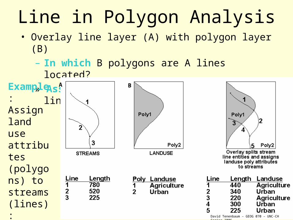
• Overlay line layer (A) with polygon layer (B)

– In which B polygons are A lines located?

» Assign polygon attributes from B to lines in A

A BExample: Assign land use attributes (polygons) to streams (lines):

Line in Polygon Analysis

David Tenenbaum – GEOG 070 – UNC-CH Spring 2005

Lecture 22

• Questions from this section are likely to be ‘problems’ – I may show you a small raster image (with numbers in each cell), and have you calculate the intersection/‘and’ or the union/‘or’ image.

0 1 1

0 0 1

1 0 1

0 0 0

1 1 1

0 0 1

AND =

Boolean Operations with Raster Layers

0 1 1

0 0 1

1 0 1

0 0 0

1 1 1

0 0 1

OR =

•The AND operation requires that the value of cells in both input layers be equal to 1 for the output to have a value of 1:

•The OR operation requires that the value of a cells in either input layer be equal to 1 for the output to have a value of 1:

101

100

110

100

111

000

+ =201

211

110

Summation

101

100

110

100

111

000

=100

100

000

Multiplication

101

100

110

100

111

000

+ =301

322

110

100

111

000

+

Summation of more than two layers

Simple Arithmetic Operations

Near the mall Near friend’s houseNear work Good place to live?

Spatial Interpolation

• You have point data (temp or air pollution levels).• You want the values across your full study site.• Spatial interpolation estimates values in areas with no

data.– creates a contour map by drawing isolines between the data

points, or– creates a raster digital elevation model which has a value for

every cell

Spatial Interpolation:Inverse Distance Weighting (IDW)

• One method of interpolation is inverse distance weighting:

• The unknown value at a point is estimated by taking a weighted average of known values

– Those known points closer to the unknown point have higher weights.

– Those known points farther from the unknown point have lower weights.

Lecture 23

In neighborhood operations, we look at a neighborhood of cells around the cell of interest to arrive at a new value.

We create a new raster layer with these new values.

A 3x3 neighborhood

Neighborhood Operations

An input layer

Cell ofInterest

• Neighborhoods of any size can be used• 3x3 neighborhoods work for all but outer edge cells

Neighborhood operations are called convolution operations.

Neighborhood Operations

• The neighborhood is often called:– A window– A filter– A kernel

– They can be applied to:• raw data (BV’s)• classified data (nominal landcover classes)

A 3x3 neighborhood

Neighborhood Operation: Majority Filter

24221

13383

13322

72325

33322

24221

13383

13322

72325

33322

24221

13883

13322

72325

33322

InputLayer

ResultLayer

2 3 3

•The majority value (the value that appears most often, also called a mode filter):

Edge Enhancement

Sharpening FilterNormal Image

Edge enhancement filters sharpen images.

The Centroid• The centroid is the spatial mean. The

‘average’ location of all points.

• The centroid can also be thought of as the balance point of a set of points.

USA Population Centroid

• Population centroid change over time in USA

Lecture 24

Landcover Pattern Metrics

• Landcover pattern metrics describe the pattern of landcover in a landscape.– Landcover fragmentation

• Average patch size• Distance between patches of the same landcover

– Patch shape • Long and thin vs. round or square• Jagged edges vs. clean edges

Location-Allocation Problems

• This class of problems in known as location-allocation problems, and solving them usually involves choosing locations for services, and allocating demand to them to achieve specified goals

• Those goals might include:– minimizing total distance traveled– minimizing the largest distance traveled by any customer– maximizing profits– minimizing a combination of travel distance and facility operating

cost

Lecture 25

• Understand the concept of supervised classification

• Understand the concept of unsupervised classification

Population Environment

• Be prepared to comment on population-environment studies that I give you on the test.