FINAL REPORT

ON

THE WATERSHED MODELING AND EDUCATION PROJECT

FOR

THE LOWER TUSCAN AQUIFER

by

S. Kure, S. Jang, N. Ohara, M. L. Kavvas

Hydrologic Research Laboratory Department of Civil and Environmental Engineering

University of California, Davis

Principal Investigator: M.L.Kavvas

Report to Butte County

April, 2010

ii

Table of Contents

1. INTRODUCTION AND OBJECTIVES................................................................................. 1

2. OVERVIEW OF THE FOOTHILLS WATERSHEDS ........................................................ 3

3. METHODOLOGY ................................................................................................................... 8

4. CRITICAL DRY AND WET PERIOD ANALYSIS ............................................................. 9

5. DEVELOPMENT OF A GEOGRAPHIC INFORMATION SYSTEM (GIS) FOR THE FOOTHILLS WATERSHEDS.............................................................................................. 14

1) DIGITAL ELEVATION MODEL (DEM) DATA .......................................................................... 14 2) WATERSHED DELINEATION AND RIVER STREAM NETWORK DATA ....................................... 14 3) VEGETATION AND LAND COVER/USE DATA............................................................................ 15 4) SOIL SURVEY DATA ............................................................................................................... 17

6. RECONSTRUCTION OF HISTORICAL HYDRO-CLIMATE DATA OVER THE FOOTHILLS REGION.......................................................................................................... 19

7. HYDROLOGIC MODELING FOR THE FOOTHILLS WATERSHEDS...................... 24

1) CONFIGURATION AND PARAMETER ESTIMATION FOR WEHY MODEL.................................... 27 2) SNOW ACCUMULATION AND MELTING PROCESS MODELING...................................................33 3) HILL -SLOPE PROCESS MODELING AND STREAM NETWORK ROUTING...................................... 37 4) MODEL EVALUATION AT THE MONTHLY TIME SCALE ............................................................. 42

8. INFLOW DATA FROM THE WATERSHEDS TO THE RECHARGE ZONE LAND SURFACE BOUNDARY OF THE IWFM GROUND WATER MODEL........................ 44

9. SUMMARY AND CONCLUSIONS ..................................................................................... 46

REFERENCES............................................................................................................................ 48

iii

List of Figures Figure 1- IWFM Hydrologic Components (BCDWRC, 2008)...................................................... 1 Figure 2- Map of the foothills watersheds that contribute to the Butte Basin Groundwater Model

................................................................................................................................................. 4 Figure 3- Vegetation and land use/cover map over the foothills watersheds ................................ 4 Figure 4- Example pictures of the foothills watersheds................................................................. 5 Figure 5- Example pictures of the creeks in the foothills watersheds ........................................... 5 Figure 6- Model domains of the WEHY model and IWFM groundwater model.......................... 6 Figure 7- Available observation stations over the foothills watersheds ........................................8 Figure 8- Watershed hydrology modeling methodology ............................................................... 9 Figure 9- Time series of the observed annual precipitation and annual mean discharge at Butte

Creek..................................................................................................................................... 10 Figure 10- Time series of the observed annual precipitation and annual mean discharge at Deer

Creek..................................................................................................................................... 11 Figure 11- Time series of the cumulative inflow at Butte Creek from 1965 through 2007......... 12 Figure 12- Time series of the cumulative inflow at Deer Creek from 1965 through 2007 ......... 12 Figure 13- Time series of the surplus inflow at Butte Creek from 1965 through 2007............... 13 Figure 14- Time series of the surplus inflow at Deer Creek from 1965 through 2007................ 13 Figure 15- Derived channel network and watershed delineations ............................................... 15 Figure 16- Local vegetation and land cover/use survey map over the foothills region published

by CaSIL ............................................................................................................................... 16 Figure 17- Example LAI maps over the foothills watersheds in 2004 ........................................ 17 Figure 18- Soil map derived from SSURGO dataset................................................................... 18 Figure 19- Depiction of four nested grids used for the MM5 simulation of the foothills

watersheds............................................................................................................................. 21 Figure 20- Comparisons of the observed and model simulated monthly precipitation at each

observation station from January 1982 through December1992 .......................................... 22 Figure 21- Comparisons of the observed and model simulated monthly mean air temperature at

each observation station from January 1984 through December1992.................................. 22 Figure 22- Comparison of model simulated precipitation field and PRISM data over the foothills

region for December 1987 .................................................................................................... 23 Figure 23- Schematic description of WEHY model .................................................................... 25 Figure 24- Structural description of WEHY model ..................................................................... 26 Figure 25- Delineated MCUs map and river stream network at each watershed ........................ 27 Figure 26- Delineated rill distribution maps at each watershed................................................... 29 Figure 27- Mean soil depth map in the foothills watersheds ....................................................... 30 Figure 28- Median of saturated hydraulic conductivity and standard deviation of log saturated

hydraulic conductivity map in the foothills watersheds ....................................................... 30 Figure 29- Mean porosity and mean residual water content map in the foothills watersheds..... 31 Figure 30- Mean bubbling pressure and mean pore size index map in the foothills watersheds. 31 Figure 31- Mean roughness height and mean root depth map in the foothills watersheds.......... 32 Figure 32- Mean albedo and mean emissivity map in the foothills watersheds .......................... 32 Figure 33- Seasonal mean LAI maps in the foothills watersheds................................................ 33 Figure 34- Sketch of spatially distributed snow model (Ohara et al. 2006) ................................ 34 Figure 35- Illustration of the approximation of snow temperature vertical profile (Ohara et al.

2006) ..................................................................................................................................... 34

iv

Figure 36- Time series of the observed and model simulated snow water equivalent at the field observation sites in the foothills region from October 2004 through September 2005 ........ 35

Figure 37- Time series of the observed and model simulated snow depth at the field observation site in the foothills region from October 2004 through September 2005 ............................. 36

Figure 38- Model simulated snow cover extent and the maximum snow extent derived with MODIS/Terra snow cover at each first day of the month over the foothills region from October 2004 through March 2005....................................................................................... 36

Figure 39- Time series of the observed and model simulated hourly stream discharge at the field observation site of the Butte Creek from October 2004 through September 2005............... 38

Figure 40- Time series of the observed and model simulated hourly stream discharge at the field observation site of the Big Chico Creek from October 2004 through September 2005 ....... 38

Figure 41- Time series of the observed and model simulated daily mean stream discharge at the field observation site of the Little Chico Creek from October 1991 through September 1992............................................................................................................................................... 39

Figure 42- Time series of the observed and model simulated hourly stream discharge at the field observation site of the Deer Creek from October 2004 through September 2005................ 39

Figure 43- Comparisons of the daily mean discharge between WEHY model simulation and observations at Butte Creek watershed from October 1982 through September 1992......... 40

Figure 44- Comparisons of the daily mean discharge between WEHY model simulation and observations at Big Chico Creek watershed from October 1982 through September 1992 . 41

Figure 45- Comparisons of the daily mean discharge between WEHY model simulation and observations at Little Chico Creek watershed from October 1982 through September 1992............................................................................................................................................... 41

Figure 46- Comparisons of the daily mean discharge between WEHY model simulation and observations at Deer Creek watershed from October 1982 through September 1992.......... 42

Figure 47- Comparisons of the monthly flow volume between WEHY model simulation and observations at Deer Creek watershed (Upper) and Big Chico Creek watershed (Lower) from October 1982 through September 1992 ....................................................................... 43

Figure 48- Comparisons of the monthly flow volume between WEHY model simulation and observations at Butte Creek watershed (Upper) and Little Chico Creek watershed (Lower) from October 1982 through September 1992 ....................................................................... 43

Figure 49- Cross points of the river stream network of the WEHY model and the model domain of the IWFM groundwater model ......................................................................................... 45

Figure 50- Inflow data from the foothills watersheds to the recharge zone land surface boundary of the IWFM groundwater model from October 1982 through October 1992 ..................... 46

v

List of Tables Table 1- Location information and data source of the ground observation stations

in the foothills region ...................................................................................... 7 Table 2- Soil texture classes and their properties (Rawls et al., 1982 and McCuen

et al., 1981) ................................................................................................... 19 Table 3- Nested grid data for the foothills region ................................................ 20 Table 4- Total number of MCUs at each watershed............................................. 28 Table 5- RMSE, Relative RMSE, and Nash-Sutcliffe Efficiency values for the

simulation results at each studied watershed. ................................................ 44

1

1. Introduction and Objectives

Percolation of infiltrated water from the watersheds into the groundwater aquifer systems of

Northern Sacramento Valley is very important for the water resources in the area. In this project

a physically based model was used to estimate the run-off from the Big Chico Creek, Little

Chico Creek, Butte Creek and Deer Creek watersheds into the groundwater aquifer system of

Butte County, which is proposed for increased pumping in order to substitute for surface water

supplied to the Sacramento Valley Water Management Agreement (SVWMA). Components of

the aquifer system underlie four counties in the northern Sacramento Valley, at the surface in

Butte and Tehama Counties and dipping to a depth of over 1000 feet below Glenn and Colusa

Counties. SVWMA parties have agreed to provide some of their surface water to improve Delta

water standards. The Lower Tuscan groundwater aquifer is envisioned as one groundwater

source for that program, as it is believed to be confined as it dips below the ground surface and is

believed to hold large quantities of groundwater. The Integrated Water Flow Model (IWFM) is

used for the Butte Basin Groundwater Model (BCDWRC, 2008). IWFM is a quasi-3 dimensional

finite-element model and a water resources management and planning model that simulates

groundwater, surface water, surface-groundwater interaction as well as other components of the

hydrologic cycle, as shown in Figure 1.

Figure 1- IWFM Hydrologic Components (BCDWRC, 2008)

2

IWFM was formerly known as IGSM2 (Integrated Groundwater and Surface water Model 2nd

generation) with a name change taking place in September 2005. IWFM was developed by the

staff in the Modeling Support Branch of California DWR’s Bay-Delta Office. IWFM is an

important water resource management tool for Butte County to complete local integrated water

resource planning.

One of the critical points in the application of the IWFM is how to determine the inflow data

from foothills watersheds into the IWFM model boundary. It is very important for the simulation

results of the groundwater model to set up the boundary inflow condition to the model domain

appropriately and accurately. The main objective of this project is to estimate the run-off from

the foothills watersheds into the IWFM ground water model boundary. The recharge estimate

provided by this project will determine the input into the IWFM and contribute to better

management of the aquifer in order to maintain local water supply reliability as the aquifer

contributes to statewide water supply reliability needs. It will assist water managers in

protecting water users and ecosystems that are dependent on groundwater levels.

One of the problems in the estimation of the run-off in the project is that there is no existing

precipitation data at some mountainous watersheds. Success in Prediction in Ungauged Basins

(PUB) is a challenging problem in Hydrology. Today in most parts of the world, a significant

amount of spatial information like remote sensing images, is available. However the hydrological

information derived from such sources cannot be a complete answer to the PUB problem. For

example, the physically based distributed hydrology models require a lot of spatially distributed

hydro-atmospheric data as the input data to the models. Atmospheric data such as precipitation,

short and long wave radiation, wind speed, relative humidity, air temperature, etc., are crucial

information in the application of a land surface parameterization or snow accumulation and

melting process modeling. However, it is very difficult to obtain the spatially distributed hydro-

atmospheric data in mountainous watersheds at fine resolution in time and space. In order to

overcome this problem, a dynamic downscaling of global reanalysis data can be used as a

powerful tool to reconstruct the hydro-atmospheric data at ungauged or sparsely gauged basins

as it enables us to apply the physically based distributed models to the basins with the spatially

distributed input data at the fine resolution.

In this project, reconstruction of historical hydro-climate data based on a regional hydro-

climate model (RegHCM) with the physically based, spatially distributed watershed

environmental hydrology (WEHY) model is applied to the foothills region in order to estimate

the run-off from the studied watersheds. Furthermore, some parts of the watersheds, especially

3

Deer Creek and Butte Creek watershed, are located at high elevation (> 2000m) and are covered

by snow during the winter seasons when snowmelt is an important contributor to the river stream

discharge during dry seasons (especially April, May, and June). Therefore, snow accumulation

and melting processes are taken into account during the watershed modeling for the precise

estimation of the runoff from these watersheds in the project.

The project, called “The Watershed Modeling and Education Project for the Lower Tuscan

Aquifer”, consisted of:

� Collection of hydrologic data over the foothills region

� Critical dry and wet periods analysis using historical hydrologic data

� Development of a geographical information system (GIS) over the foothills region

� Reconstruction of historical hydro-climate data over the foothills region

� Snow accumulation and melting process modeling

� WEHY Model implementation, calibration and validation for the foothills watersheds

� Estimation of inflow data from the watersheds to the recharge zone land surface boundary of

the IWFM groundwater model

2. Overview of the Foothills Watersheds

The foothills watersheds, Big Chico Creek, Little Chico Creek, Butte Creek and Deer Creek

watersheds, in Northern California were selected in the project as shown in Figure 2. The

watersheds are located at the foothills and are covered by various vegetation types through

elevations from 86 m to 1,798m (Big Chico Creek watershed), from 87m to 1065m (Little Chico

Creek watershed), from 69m to 2187m (Butte Creek watershed) and from 150m to 2390m (Deer

Creek watershed), so that the land use/cover of this area is geophysically and biologically

heterogeneous. Figure 3 shows the land cover and vegetation map obtained from Multi-source

Land Cover Data in the foothills region, published by California Spatial Information Library

(CaSIL), with a USGS land use classification. The watersheds are mainly covered by vegetation

such as the ever green needle leaves, deciduous broad leaves, and so on. Figure 4 and 5 show

example pictures of the watersheds. It can be seen from Figure 4 that some open spaces can be

4

found in the lower sectors of the watersheds. The run-off from these watersheds is simulated

using the WEHY model in the project, and is used as input into the IWFM groundwater model,

as discussed later. Figure 6 shows the model domains of the IWFM and WEHY model.

30 0 30 60 Miles

N

EW

S

Figure 2- Map of the foothills watersheds that contribute to the Butte Basin Groundwater Model

GrasslandIrrigated Cropland PastureBarren or Sparsely VegetatedDecids. Broadleaf ForestShrublandEvergreen NeedleafWater bodiesHerbaceous WetlandUrban

Figure 3- Vegetation and land use/cover map over the foothills watersheds

5

Figure 4- Example pictures of the foothills watersheds

Figure 5- Example pictures of the creeks in the foothills watersheds

6

13 - 245245 - 478478 - 711711 - 943943 - 11761176 - 14091409 - 16411641 - 18741874 - 21072107 - 23392339 - 25722572 - 2805No Data

Elevation [m]

: IWFM ground water model domain : WEHY model domain

: River stream

Deer Creek Watershed

Upper Butte Creek WatershedBig Chico

Creek Watershed Little Chico

Creek Watershed

Figure 6- Model domains of the WEHY model and IWFM groundwater model.

Historical records of hydrologic ground observation data are indispensable for the model

calibration and validation processes. Various data sources were searched in order to collect the

publicly available information on historical atmospheric data. 13 stations from California Data

Exchange Center (CDEC) of CDWR and 1 station at the Little Chico Creek from CDWR

Northern District for the precipitation, stream discharge, and snow data were found in the project

area (Table 1). Figure 7 shows the digital elevation map with the ground observation station

points over the watersheds. Some observation stations can be found in the area, but there is no

precipitation station in the Deer Creek and Big Chico Creek watersheds. Furthermore, there are

only two stations (DES and CAR) which provide hourly precipitation over the watersheds. In

general, there are a few meteorological observation stations at the mountainous watersheds

compared to the valley or urban areas. It should be emphasized that the importance of the spatial

variability of precipitation on the runoff hydrograph has been long recognized and the orographic

precipitation is a well-known and common phenomenon in Sierra Nevada. The effects of spatial

distribution of the precipitation due to the orographic characteristics should be considered for the

input precipitation data to the watershed models applied to the high elevation area. The ground

7

observation stations are usually installed in the valleys of the watershed for easy access,

maintenance and installation, so that a basin average precipitation based on the ground

observation data tends to miss the high intensity precipitation observed at the hilltops of the

watershed. For the physically based, spatially distributed land surface parameterization and snow

accumulation and melting process modeling, a lot of spatially distributed hydro-meteorologic

data such as precipitation, air temperature, relative humidity, wind speed, short and long wave

radiation etc., are required. However, it is difficult to find spatially distributed hydro-

meteorologic data at the mountainous watersheds at fine resolution in time and space. In order to

reconstruct the historical hydro-climate data over the foothills region at the fine spatial resolution,

a dynamic downscaling is utilized in this project. Because regional climate models, employed for

the dynamic downscaling, simulate the physical atmospheric processes locally, the regional

climate features such as orographic precipitation and extreme climate events can be simulated by

these models. Furthermore, this downscaling approach makes it possible to apply the physically

based, distributed hydrologic models to the ungauged and heterogeneous basins.

Table 1- Location information and data source of the ground observation stations in the foothills region

Station IDStation IDStation IDStation ID Station NameStation NameStation NameStation Name XXXX YYYY Z (m)Z (m)Z (m)Z (m) Data SourceData SourceData SourceData Source DataDataDataData

DCVDCVDCVDCV DEER CREEK NR VINA -121.947 40.014 146 CDEC Discharge

BIGBIGBIGBIG BIG MEADOW (KERN CO) -121.777 39.768 2359 CDEC Discharge

BCKBCKBCKBCK BUTTE CREEK NR CHICO -121.709 39.726 91 CDEC Discharge

A40280A40280A40280A40280 A40280 -121.770 39.750 129 DWRND Discharge

BTMBTMBTMBTM BUTTE MEADOWS -121.500 40.100 1487 CDEC Precipitation

CARCARCARCAR CARPENTER RIDGE -121.582 40.069 1467 CDEC Precipitation

DESDESDESDES DE SABLA (DWR) -121.610 39.872 826 CDEC Precipitation

DSBDSBDSBDSB DE SABLA (PG&E) -121.617 39.867 826 CDEC Precipitation

PRDPRDPRDPRD PARADISE FIRE STATION -121.617 39.750 533 CDEC Precipitation

CSTCSTCSTCST COHASSET -121.771 39.875 488 CDEC Precipitation

CHICHICHICHI CHICO -121.783 39.712 70 CDEC Precipitation

CESCESCESCES CHICO UNIV FARM -121.817 39.700 56 CDEC Precipitation

HMBHMBHMBHMB HUMBUG -121.368 40.115 1981 CDEC Snow

FEMFEMFEMFEM FEATHER RIVER MEADOW -121.422 40.355 1646 CDEC Snow

8

$T

$T

$T$T

$T

$T

$T$T

%U

%U

#S

#S

#S#S

DCV

BIG

A40280

BCK

FEM

HMB

BTM

CAR

DESDSB

PRD

CST

CHICES

Elevation [m]48 - 309309 - 570570 - 831831 - 10911091 - 13521352 - 16131613 - 18741874 - 21342134 - 2395

Deer Creek watershed (508km2)

Upper Butte Creek watershed (407km2)

Little Chico Creek watershed (78km2)

Big Chico Creek watershed (192km2)

●: Discharge stations (CDEC)▲: Precipitation stations (CDEC)□: Snow stations (CDEC)

:Hourly Precipitation

Figure 7- Available observation stations over the foothills watersheds

3. Methodology

In order to estimate the run-off from the foothills watersheds to the recharge zone land surface

boundary of the IWFM ground water model for the Lower Tuscan Aquifer system, all the

hydrologic processes in the watersheds must be modeled properly. The physically-based (or

process-based) modeling approach for the hydrological processes is required in order to simulate

the river stream discharge at the ungauged or sparsely gauged basins. For this project, several

model layers, shown in Figure 8, were organized and implemented: a regional hydroclimate

model, a snow accumulation and melting model, a hillslope process model, and a river channel

routing model. The modeled hydrologic quantities are calibrated and validated by the field-

monitored data at every modeling step.

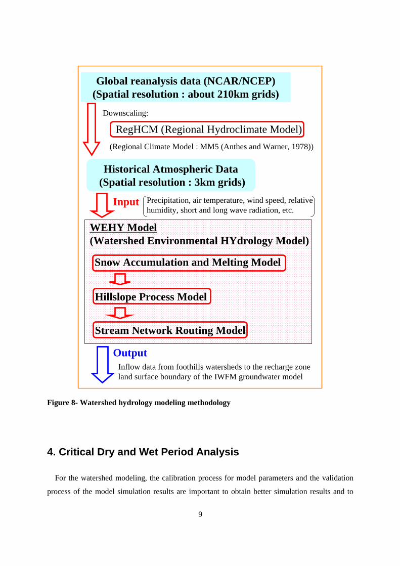
9

Historical Atmospheric Data(Spatial resolution : 3km grids)

Global reanalysis data (NCAR/NCEP) (Spatial resolution : about 210km grids)

Downscaling:

(Regional Climate Model : MM5 (Anthes and Warner, 1978))

RegHCM (Regional Hydroclimate Model)

WEHY Model (Watershed Environmental HYdrology Model)

Input

Snow Accumulation and Melting Model

Hillslope Process Model

Stream Network Routing Model

Inflow data from foothills watersheds to the recharge zone land surface boundary of the IWFM groundwater model

Precipitation, air temperature, wind speed, relative humidity, short and long wave radiation, etc.

Output

Figure 8- Watershed hydrology modeling methodology

4. Critical Dry and Wet Period Analysis

For the watershed modeling, the calibration process for model parameters and the validation

process of the model simulation results are important to obtain better simulation results and to

10

evaluate the model performance and reliability. In general, some model parameters need to be

adjusted by trial and error to improve model simulation results. Then the calibrated model for the

intended area should be checked for its reliability and performance based on the observed data

during the validation period. It is important that the model should be able to simulate not only the

usual average condition of the watersheds but also the critical wet and dry periods, which include

the extreme flood and drought events, with the calibrated and averaged parameters of the model.

These critical dry and wet years are very important for the watersheds’ management, flood

prediction, water supply, and so on.

In order to identify the dry and wet years of the foothills watersheds, critical dry and wet

period analysis was performed using the historical stream flow and precipitation data at Butte

Creek and Deer Creek watersheds. Figure 9 and Figure 10 show the time series of the observed

annual mean river stream discharge and annual precipitation data at the Butte Creek and Deer

Creek.

1910 1920 1930 1940 1950 1960 1970 1980 1990 20000

10

20

303000

2000

1000

0

Ann

ual M

ean

Dis

char

ge [m

3 /s] a

t CH

ICO

Ann

ual P

reci

pita

tion

[mm

] at D

SB

Date [Year]

Ave:1591.2mm

Ave:11.8m3/s

Wet(82–83)

Dry(87–92)

Figure 9- Time series of the observed annual precipitation and annual mean discharge at Butte Creek

11

1910 1920 1930 1940 1950 1960 1970 1980 1990 20000

10

20

303000

2000

1000

0

Ann

ual M

ean

Dis

char

ge [m

3 /s] a

t VIN

A

Ann

ual P

reci

pita

tion

[mm

] at D

SB

Date [Year]

Ave:1591.2mm

Ave:9.2m3/s

Wet(82–83)

Dry(87–92)

Figure 10- Time series of the observed annual precipitation and annual mean discharge at Deer Creek

It is seen from Figure 9 and Figure 10 that the largest discharge value is found in 1983. It is

also found that the consecutive dry years are observed from 1987 through 1992. It should be

noted that there is the smallest annual mean discharge value in 1977. However, from the point of

view of the water resource management, consecutive dry years are more difficult to manage the

water supply for the irrigation and drinking water uses. Therefore, continuous dry years from

1987 through 1992 were selected as the critical dry period for the model validation.

Figure 11 and Figure 12 show the time series of the accumulative river discharge at Butte

Creek and Deer Creek from 1965 through 2007. In these figures steep gradients mean wet years

and mild gradients mean dry years.

12

0

20

40

60

80

100

120

Jan, 1965

Jan, 1966

Jan

, 1967

Jan, 1968

Jan, 1969

Jan

, 1970

Jan

, 1971

Jan, 1972

Jan, 1973

Jan

, 1974

Jan, 1975

Jan, 1976

Jan

, 1977

Jan

, 1978

Jan, 1979

Jan, 1980

Jan

, 1981

Jan, 1982

Jan, 1983

Jan

, 1984

Jan

, 1985

Jan, 1986

Jan

, 1987

Jan

, 1988

Jan, 1989

Jan, 1990

Jan

, 1991

Jan

, 1992

Jan, 1993

Jan

, 1994

Jan

, 1995

Jan, 1996

Jan, 1997

Jan

, 1998

Jan

, 1999

Jan, 2000

Jan

, 2001

Jan

, 2002

Jan, 2003

Jan, 2004

Jan

, 2005

Jan, 2006

Jan, 2007

十十十十

万万万万

Date

Cum

ula

tive

flo

w (

af)

Accumulated flow

Average line

1976-1977

1983

1995

1987-1992

Dry

Dry

Wet

Wet

(×100,000)

Figure 11- Time series of the cumulative inflow at Butte Creek from 1965 through 2007

0

20

40

60

80

100

120

Jan, 1965

Jan, 1966

Jan

, 1967

Jan, 1968

Jan, 1969

Jan

, 1970

Jan

, 1971

Jan, 1972

Jan, 1973

Jan

, 1974

Jan, 1975

Jan, 1976

Jan

, 1977

Jan

, 1978

Jan, 1979

Jan, 1980

Jan

, 1981

Jan, 1982

Jan, 1983

Jan

, 1984

Jan

, 1985

Jan, 1986

Jan

, 1987

Jan

, 1988

Jan, 1989

Jan, 1990

Jan

, 1991

Jan

, 1992

Jan, 1993

Jan

, 1994

Jan

, 1995

Jan, 1996

Jan, 1997

Jan

, 1998

Jan

, 1999

Jan, 2000

Jan

, 2001

Jan

, 2002

Jan, 2003

Jan, 2004

Jan

, 2005

Jan, 2006

Jan, 2007

十十十十

万万万万

Date

Cum

ula

tive

flo

w (

af)

Accumulated flow

Average line

1976-1977

1983

1995

1987-1992Dry

DryWet

Wet

(×100,000)

Figure 12- Time series of the cumulative inflow at Deer Creek from 1965 through 2007

Figures 13 and 14 show the time series of the surplus value of the river discharge from

averaged flow at Butte Creek and Deer Creek from 1965 through 2007. If the accumulated

discharge line is above the horizontal axis (average line), it means the cumulative water resource

has surplus and the period can be identified as wet year. From the Figures 13 and 14, it can be

clearly seen that the dry years from 1987 through 1992 define a critically dry period as the

cumulative discharge line is far below the average line. Thus, we determined that 1982-1983 was

13

the critical wet period, and 1987-1992 was the critical dry period, the modeling effort was

focused on for model validation. Furthermore, the period from 2004 through 2005 was selected

for the calibration period of the model since abundant data, especially hourly time increment data,

are available during the period. Surplus flow at BUTTE NR CHICO from 1947 to 2008

-8.00

-6.00

-4.00

-2.00

0.00

2.00

4.00

6.00

Jan

, 1965

Jan, 1966

Jan, 1967

Jan

, 1968

Jan, 1969

Jan, 1970

Jan

, 1971

Jan

, 1972

Jan, 1973

Jan, 1974

Jan

, 1975

Jan

, 1976

Jan, 1977

Jan, 1978

Jan

, 1979

Jan

, 1980

Jan, 1981

Jan

, 1982

Jan

, 1983

Jan, 1984

Jan, 1985

Jan

, 1986

Jan

, 1987

Jan, 1988

Jan, 1989

Jan

, 1990

Jan

, 1991

Jan, 1992

Jan

, 1993

Jan

, 1994

Jan, 1995

Jan, 1996

Jan

, 1997

Jan

, 1998

Jan, 1999

Jan, 2000

Jan

, 2001

Jan

, 2002

Jan, 2003

Jan, 2004

Jan

, 2005

Jan, 2006

Jan, 2007

十十十十

万万万万

Date

Surp

lus

flow [

Cum

-Q

- A

vera

ge] (a

f)

1976-1977

1983

1995

Dry Wet

Wet

1987-1992Dry

(×100,000)

Figure 13- Time series of the surplus inflow at Butte Creek from 1965 through 2007 Surplus flow at DEER C NR VINA from 1965 to 2008

-6.00

-4.00

-2.00

0.00

2.00

4.00

6.00

Jan

, 1965

Jan, 1966

Jan, 1967

Jan

, 1968

Jan, 1969

Jan, 1970

Jan

, 1971

Jan

, 1972

Jan, 1973

Jan, 1974

Jan

, 1975

Jan

, 1976

Jan, 1977

Jan, 1978

Jan

, 1979

Jan

, 1980

Jan, 1981

Jan

, 1982

Jan

, 1983

Jan, 1984

Jan, 1985

Jan

, 1986

Jan

, 1987

Jan, 1988

Jan, 1989

Jan

, 1990

Jan

, 1991

Jan, 1992

Jan

, 1993

Jan

, 1994

Jan, 1995

Jan, 1996

Jan

, 1997

Jan

, 1998

Jan, 1999

Jan, 2000

Jan

, 2001

Jan

, 2002

Jan, 2003

Jan, 2004

Jan

, 2005

Jan, 2006

Jan, 2007

十十十十

万万万万

Date

Surp

lus

flow [

Cum

-Q

- A

vera

ge] (a

f)

1983

1995

1976-1977Dry Wet

1987-1992Dry

(×100,000)

Wet

Figure 14- Time series of the surplus inflow at Deer Creek from 1965 through 2007

14

5. Development of a Geographic Information System (GIS) for the Foothills Watersheds

In order to support watershed modeling, a geographic information system (GIS) was

established for the project. The geo-referenced data, including spatially distributed data and point

data from various sources were downloaded and processed. The Universal Transverse Mercator

(UTM) coordinate system was selected as the standard GIS coordinate system for the Project.

The Universal Transverse Mercator Coordinate system divides the World into 60 zones, each

being 6 degrees longitude wide, and extending from 80 degrees south latitude to 84 degrees north

latitude. The UTM “ZONE 10” projection is used for the project. If the original dataset is not in

the selected coordinate system, it is re-projected into the UTM “ZONE 10” coordinates. All the

geo-referenced datasets in this project have been defined in this coordinate system. An example

GIS map in Figure 2 shows geophysical elevation, the locations of cities, stream channels,

county boundaries, and the watershed boundary for the foothills watersheds.

It should be emphasized that the vegetation parameters are crucial for the land surface

parameterizations and snow models, and seasonal and spatial variabilities of these parameters

should be considered for the modeling. Recent advances in remote sensing techniques and

advanced GIS database and tools enable us to obtain the spatial and temporal properties of land

surface parameters.

1) Digital Elevation Model (DEM) Data

The digital elevation model (DEM) data at 1 arc second resolution that corresponds to about

30 meter resolution, was downloaded from the Seamless Data Center of USGS and processed for

the foothill watersheds and its adjacent regions. It was re-projected into UTM ZONE10

coordinates by utilizing a projection extension of ArcView software. The final processed DEM

was also clipped in order to cover only the project area.

2) Watershed Delineation and River Stream Network Data

15

Based upon the DEM at about 30 m resolution by USGS, delineation of the watersheds was

carried out for the foothills watersheds using the Arc View tools. The derived channel network

and watershed delineations, based on the reconditioned DEM, are shown in Figure 15.

10 - 320320 - 630630 - 950950 - 12601260 - 15701570 - 18801880 - 21902190 - 25002500 - 2810No Data

Basin boundariesRiver Stream

Elevation [m]

N

EW

S

Figure 15- Derived channel network and watershed delineations

3) Vegetation and Land Cover/use Data

From vegetation and land cover/use data the parameters such as the roughness height, surface

albedo, emissivity and vegetation root depth for the land surface parameterization and snow

model are determined. These vegetation parameters are important to calculate the

evapotranspiration and snow accumulation and melting in the land surface processes. For the

vegetation data Multi-source Land Cover Data based upon the local survey, published by CaSIL,

which has 100 m spatial resolution, was employed and implemented into the foothill watersheds

GIS system, as shown in Figure 16. Furthermore, the effective rooting depth of the vegetations

was estimated from the vegetation types and land cover/use by means of Gale and Grigal (1987).

16

WTMWFRWATVRIVOWURBSMCSGBSEWSCNRIVRFRRDWPPNPOSPJNPGS

MRI

MHW

MHCMCPMCHMARLSGLPN

LACKMCJUNJSTJPNFEWESTEPNDSWDSSDSCDRIDFRCSCCRCCPC COW

BOW

BOP

BBRBARASPASCAGS

Figure 16- Local vegetation and land cover/use survey map over the foothills region published by CaSIL

Leaf Area Index (LAI) is defined as the amount of leaf area (m2) in a canopy per unit ground

area (m2) and is very important for the evapotranspiration and snow accumulation and melting

processes. The monthly LAI derived by MODIS (MODerate resolution Imaging

Spectroradiometer; Wolfe et al. 1998 and so on) satellite images were obtained at a spatial grid

resolution of 1 km x 1km. Figure 17 shows example LAI maps over the foothills watersheds in

2004.

17

Observed Leaf Area Index MODIS/Aqua (MYD15)

Feb, 2004 May, 2004 Aug, 2004 Nov, 2004

LAI (Scaling factor:0.1)0 - 22 - 33 - 44 - 55 - 1010 - 2020 - 3030 - 4040 - 70No Data

Figure 17- Example LAI maps over the foothills watersheds in 2004

4) Soil Survey Data

Water flow in soils is modeled mathematically by a combination of the mass conservation

equation, Darcy’s law, the soil water retention relationship, and water saturation versus hydraulic

conductivity relationship in WEHY model (Chen et al. 1994 a,b, Kavvas et al. 2004, Chen et al.

2004 a,b). There are a total of 6 soil hydraulic parameters that need to be estimated for WEHY

model: 1) mean of volumetric water content at saturation, 2) mean of residual volumetric water

content, 3) mean of bubbling pressure head, 4) mean of pore size distribution index, 5) mean of

saturated hydraulic conductivity, and 6) variance of saturated hydraulic conductivity.

These soil parameters were estimated by means of the USDA Soil Survey Geographic

database called “SSURGO” (Soil Conservation Service, 1991) which has the finest available

spatial resolution over the project area, shown in Figure 18, and by the relationships between

18

soil texture and soil hydraulic parameters (Rawls et al., 1982 and McCuen et al., 1981), shown in

Table 2. Different colors represent the different soil types in Figure 18. From the SSURGO data

set and soil texture table soil parameters such as the soil depth, saturated hydraulic conductivity,

total porosity, pore size distribution index, bubbling pressure, and residual saturation in terms of

their depth averages can be obtained.

basin boundariesRiver Stream

Figure 18- Soil map derived from SSURGO dataset

19

Table 2- Soil texture classes and their properties (Rawls et al., 1982 and McCuen et al., 1981)

Mean Sat. hydraulic conduct.

SD of Sat. hydraulic conduct.

Mean Total

Porosity

Mean Residual

Saturation

Mean Bubbling Pressure

Mean Pore Size Dist.

Index Soil texture class

(cm/h) (cm/h) (cm) 1 Sand 21.00 1.66 0.437 0.020 15.98 0.694 2 Loamy sand 6.11 1.24 0.437 0.035 20.58 0.553 3 Sandy loam 2.59 1.17 0.453 0.041 30.20 0.378 4 Loam 1.32 1.33 0.463 0.027 40.12 0.252 5 Silt loam 0.68 1.15 0.501 0.015 50.87 0.234 6 Sandy clay oam 0.43 1.20 0.398 0.068 59.41 0.319 7 Clay loam 0.23 1.20 0.464 0.075 56.43 0.242 8 Silty clay loam 0.15 1.16 0.471 0.040 70.33 0.177 9 Sandy clay 0.12 1.51 0.430 0.109 79.48 0.223 10 Silty clay 0.09 1.48 0.479 0.056 76.54 0.150 11 Clay 0.06 1.26 0.475 0.090 85.60 0.165

12 Organic 1.32 1.33 0.463 0.027 40.12 0.252

6. Reconstruction of Historical Hydro-climate Data over the Foothills Region

In order to apply the physically based, spatially distributed watershed models for the

ungauged or sparsely gauged basins, historical atmospheric data over the investigated area

should be reconstructed. However, for example, the U.S. National Center for Atmospheric

Research/National Center for Environmental Prediction (NCAR/NCEP) global reanalysis

atmospheric data resolution is approximately 210km in the horizontal directions, and in 6-hour

time intervals. These data are too coarse for watershed hydrologic modeling. Hence, it is

necessary to downscale and process these data in order to reconstruct historical precipitation data

over the foothills region at the scale of few kilometers (~3km) for the watershed modeling. A

regional hydrologic-atmospheric model (RegHCM) can be used for the dynamic downscaling of

the historical global reanalysis atmospheric data to foothills region at fine spatial resolution for

utilization in the watershed modeling. The model has already been used at various watersheds in

the world, and has been tested and validated over those watersheds by the UC Davis group

(Kavvas et al. 1998, Yoshitani et al. 2002, Anderson et al. 2007, Ohara et al. 2007, Yoshitani et

20

al. 2009, Jang et al. 2010). An atmospheric component of the RegHCM is MM5 (Fifth

Generation Mesoscale Model; Anthes and Warner 1978). MM5 is a nonhydrostatic model which

can be downscaled even to 1km spatial resolution. Hence, it is able to capture the impact of steep

topography and land surface/land use conditions of watersheds on the local atmospheric

conditions.

The global reanalysis data products used for this project are atmospheric data (pressure, wind,

relative and specific humidity, temperature, and potential temperature) at 6-h intervals over the

foothills watersheds and surrounding land and ocean provided by NCEP/NCAR. These data are

used as initial and boundary conditions for the RegHCM. In this project, four one-way nested

grids were set up within the model to create a downscaling from about the 210×210 km scale

reanalysis data to the 3×3 km scale over the foothills watersheds. Figure 19 shows the spatial

extent of the four nested domains for the RegHCM simulation of the foothills region, and Table

3 lists domain size and grid resolution data. Each nested domain has a spatial resolution of 1/3 of

the parent grid and focuses more on the project area of the foothill watersheds. The 1/3 ratio is

recommended in the user documentation for MM5 (Grell et al. 1994). The first domain has a

spatial grid resolution of 81 km, the second 27 km, the third 9 km, and the fourth 3 km. This

series of nested grids allows the large-scale archived atmospheric data to be economically

downscaled to the region of interest at the desired resolution.

Table 3- Nested grid data for the foothills region

Domain Grid resolution

(km) Number of grids

Domain area (㎢)

1 81 26×26 4,435,236

2 27 26×26 492,804

3 9 26×26 54,756

4 3 26×26 6,084

21

Figure 19- Depiction of four nested grids used for the MM5 simulation of the foothills watersheds.

Figure 20 shows the comparisons of the observed and model simulated monthly precipitation

at each observation station during the January 1982 – December 1992 period. Figure 21 shows

the comparisons of the observed and model simulated monthly mean air temperature at each

observation station during the January 1984 – December 1992 period. It is seen from these

figures that the observed and simulated precipitation and mean air temperature matched very

well at monthly time scale.

22

0

250

500

750

10000

250

500

750

10000

250

500

750

1000M

onth

ly P

reci

pita

tion

[mm

]：Sim.：Obs.

Jan., 1982 Jan., 1984 Jan., 1986 Jan., 1988 Jan., 1990 Jan., 1992

CES (56m)

Miss. (Obs.)

Miss. (Obs.)

PRD (533m)

DES (826m)

Figure 20- Comparisons of the observed and model simulated monthly precipitation at each observation station from January 1982 through December1992

0

10

20

30

0

10

20

30

Air

Tem

pera

ture

[℃]

Jan. 1984 Jan. 1986 Jan. 1988 Jan. 1990 Jan. 1992

：Obs.

：Sim.BTM (1487m)

CST (488m)

Figure 21- Comparisons of the observed and model simulated monthly mean air temperature at each observation station from January 1984 through December1992

23

Figure 22 shows a comparison between the model simulated precipitation field and PRISM

(Parameter-elevation Regressions on Independent Slopes Model) data over the foothills region

for December 1987. PRISM data sets, developed by Oregon State University, provide

interpolated ground precipitation observation data that have 4km spatial resolution and monthly

time intervals over USA from 1895 to present.

MM5 (3km) PRISM (4km)

●:Rain gauges

Pre. [mm]

% 0 - 100% 100 - 200% 200 - 300% 300 - 400% 400 - 500% 500 - 600% 600 - 700% 700 - 800% 800 - 900% 900 - 1000% 1000 - 1100

Figure 22- Comparison of model simulated precipitation field and PRISM data over the foothills region for December 1987

MM5 simulation and PRISM precipitation fields are similar both with respect to magnitude

and spatial distribution. However, reconstructed precipitation fields show high intensity

precipitation structures around the high elevation area due to the orographic effects while PRISM

data do not show these structures. The reason is that the precipitation fields of PRISM data are

based on the data interpolation of the ground observation stations which usually are installed in

the valleys of the watershed for easy access, maintenance and installation, so that PRISM data

tends to miss the high intensity precipitation observed at the hilltops of the watershed. This

comparison supports the advantage of the dynamic downscaling based on the RegHCM

employed in this project. These results related to the dynamic downscaling of NCAR/NCEP

reanalysis data are quite encouraging for the watershed modeling in the foothills region.

24

7. Hydrologic Modeling for the Foothills Watersheds

The WEHY model that utilizes upscaled hydrologic conservation equations to account for the

effect of heterogeneity within natural watersheds was applied to Deer Creek, Butte Creek, Big

Chico Creek and Little Chico Creek watersheds. WEHY model is a physically based spatially

distributed watershed hydrology model that is based upon upscaled conservation equations for

interception, snow accumulation/snowmelt, evapotranspiration, infiltration, unsaturated flow,

subsurface stormflow, overland flow, channel network flow, and regional groundwater flow. A

schematic description of the WEHY model is shown in Figure 23. A structural description of the

WEHY model is shown in Figure 24.

25

Figure 23- Schematic description of WEHY model (Kavvas et al. 2004)

26

Figure 24- Structural description of WEHY model (Kavvas et al. 2004)

The emerging parameters in the WEHY model are areal averages and areal

variance/covariances of the original point-scale parameter values. It is possible to implement and

use WEHY model at any ungauged or sparsely gauged watershed since its parameters are

estimated directly from the land features of the watershed. WEHY model can be used either for

event-based runoff prediction, or for long-term continuous-time runoff prediction. Detailed

descriptions of the WEHY model have been given previously elsewhere (Kavvas et al. 2004,

Chen et al. 2004a, b, Kavvas et al. 2006).

In order to validate the model applicability and reliability, calibration and validation periods

were selected for the application of the model based on the critical dry and wet periods analysis,

described in the earlier chapter. The calibration period is the hydrologic year from October 2004

to September 2005 and the validation period is the hydrologic years from October 1982 through

September 1992. The validation period includes critically dry and wet years in Northern

California.

27

1) Configuration and Parameter Estimation for WEHY Model

As may be seen from Figure 24, the WEHY model subdivides a watershed first into model

computational units (MCUs) that are delineated from the DEM of the watershed by means of a

geographic information system analysis (see Chen et al. 2004a). Delineated MCUs map and river

stream network at each watershed are shown in Figure 25, and the total number of MCUs at

each watershed are listed in Table 4.

Deer Creek Watershed

Upper Butte Creek Watershed

Big Chico Creek Watershed

Little Chico Creek Watershed

Figure 25- Delineated MCUs map and river stream network at each watershed

28

Table 4- Total number of MCUs at each watershed

WatershedsCatchmentArea (km2)

Total Number of MCU

Mean MCU Size (km2)

Big Chico Creek Watershed 192 54 3.6

Little Chico Creek Watershed 78 77 1.0

Deer Creek Watershed 508 94 5.4

Butte Creek Watershed 407 92 4.4

These MCUs are either individual hillslopes or first-order watersheds. The WEHY model

computes the surface and subsurface hillslope hydrologic processes that take place at these

MCUs, in parallel and simultaneously. These computations yield the flow discharges to the

stream network and the underlying unconfined groundwater aquifer of the watershed that are in

dynamic interaction both with the surface and subsurface hillslope processes at MCUs as well as

with each other (as may be seen in Figures 23 and 24). These discharged flows are then routed

by means of the stream network and the unconfined groundwater aquifer routing.

Parameters of each stream reach and of each MCU are estimated directly from the GIS

database of the watersheds, which contains information about the physical characteristics of the

watersheds. Estimation of the geomorphologic, soil hydraulic and vegetation parameters for

MCUs of the WEHY model, as was described by Chen et al. (2004a) in detail, was performed by

first overlaying the boundaries of the MCUs on the DEM map, the soil class map, and the

vegetation class map. These maps were already implemented as the GIS dataset into the

watersheds, described in the earlier chapter. Then all of the parameters of an MCU were

retrieved from the GIS data that are associated with the grid cells inside the boundary of that

MCU. As explained in the paper br Chen et al. (2004a), stationary heterogeneity of parameters

within a hillslope was assumed. Consequently, the same mean and variance values of the

parameters at the hillslope scale were used for all transects within that hillslope.

Geomorphologic parameters for the delineated stream reaches and MCUs in the WEHY model

for the foothills watershed were obtained using the general procedures described in Chen et al.

(2004a) and the foothills watersheds GIS database. The geomorphologic parameters define the

flow domains and the configurations of rills and interrill areas for MCUs of the WEHY model

for the foothills watershed. Figure 26 shows the delineated rill distributions at each watershed.

29

Deer Creek Watershed (508km2) Big Chico Creek Watershed (192km2)

:River stream

:Rill

:MCU boundary

Little Chico Creek Watershed (78km2) Upper Butte Creek Watershed (407km2)

Figure 26- Delineated rill distribution maps at each watershed

Figures 27-30 show the soil parameters of the WEHY model at each MCU. Figures 31 and

32 show the vegetation parameters of the WEHY model at each MCU. Furthermore, seasonal

LAI maps over the foothills region were developed from the satellite remote sensed data

(MODIS). Figure 33 shows the monthly mean LAI values at each watershed at every month.

Besides the geomorphologic parameters, the soil hydraulic parameters and vegetation parameters

shown in Figures 26-33, other model parameters, such as Chézy coefficients for stream reaches

and MCUs, also need to be evaluated in order to run the model. The Chézy coefficients were first

taken to be 2 (ft1/2/s) for overland flow, 5 for rill flow, and 10–25 (ft1/2/s) for the main stream

channel flow and these values were calibrated based on the observed river discharge data.

30

40 - 5050 - 6060 - 7070 - 8080 - 9090 - 100100 - 110110 - 120120 - 130130 - 140140 - 150150 - 160160 - 170170 - 180180 - 190190 - 200200 - 210

Mean depth (cm)

Figure 27- Mean soil depth map in the foothills watersheds

1 - 1.21.2 - 1 .41.4 - 1 .61.6 - 1 .81.8 - 22 - 2.22.2 - 2 .42.4 - 2 .62.6 - 2 .82.8 - 33 - 3.23.2 - 3 .43.4 - 3 .63.6 - 3 .83.8 - 44 - 4.24.2 - 4 .44.4 - 4 .64.6 - 4 .84.8 - 10

Median of Ks(cm/h)

0.2 - 0.30.3 - 0.40.4 - 0.50.5 - 0.60.6 - 0.70.7 - 0.80.8 - 0.90.9 - 11 - 1.11.1 - 1.21.2 - 1.31.3 - 1.41.4 - 1.51.5 - 1.61.6 - 1.71.7 - 1.81.8 - 1.91.9 - 22 - 2.1

SD of log Ks((cm/h)2)

Figure 28- Median of saturated hydraulic conductivity and standard deviation of log saturated hydraulic conductivity map in the foothills watersheds

31

0.42 - 0.4250.425 - 0.430.43 - 0.4350.435 - 0.440.44 - 0.4450.445 - 0.450.45 - 0.4550.455 - 0.460.46 - 0.4650.465 - 0.470.47 - 0.4750.475 - 0.480.48 - 0.4850.485 - 0.490.49 - 0.4950.495 - 0.50.5 - 0.5050.505 - 0.52

Mean porosity

0.02 - 0.02250.0225 - 0.0250.025 - 0.02750.0275 - 0.030.03 - 0.03250.0325 - 0.0350.035 - 0.03750.0375 - 0.040.04 - 0.04250.0425 - 0.0450.045 - 0.04750.0475 - 0.050.05 - 0.05250.0525 - 0.0550.055 - 0.05750.0575 - 0.060.06 - 0.06250.0625 - 0.0650.065 - 0.06750.0675 - 0.070.07 - 0.0730.073 - 0.075

Mean residual water content

Figure 29- Mean porosity and mean residual water content map in the foothills watersheds

22 - 2424 - 2626 - 2828 - 3030 - 3232 - 3434 - 3636 - 3838 - 4040 - 4242 - 4444 - 4646 - 4848 - 5050 - 5252 - 5454 - 5656 - 5858 - 6060 - 65

Mean bubbling pressure (cm)

0.2 - 0.220.22 - 0.240.24 - 0.260.26 - 0.280.28 - 0.30.3 - 0.320.32 - 0.340.34 - 0.360.36 - 0.380.38 - 0.40.4 - 0.420.42 - 0.440.44 - 0.460.46 - 0.480.48 - 0.50.5 - 0.52

Mean pore size index

Figure 30- Mean bubbling pressure and mean pore size index map in the foothills watersheds

32

Mean Roughness Height (cm)

0 - 66 - 1212 - 1818 - 2626 - 3232 - 3838 - 4646 - 52No Data

Mean Root Depth (cm)

30 - 4040 - 5050 - 6060 - 7070 - 8080 - 9090 - 100No Data

Figure 31- Mean roughness height and mean root depth map in the foothills watersheds

Mean Albedo (%)

12 - 1414 - 1616 - 1818 - 2020 - 2222 - 2424 - 2626 - 30No Data

Mean Emissivity (%)

85 - 8787 - 8989 - 9191 - 9393 - 9595 - 9797 - 99No Data

Figure 32- Mean albedo and mean emissivity map in the foothills watersheds

33

Jan. Feb. Mar. Apr.

May. Jun. Jul. Aug.

Sep. Oct. Nov. Dec.

0 - 0.50.5 - 11 - 1.51.5 - 22 - 2.52.5 - 33 - 3.53.5 - 44 - 5No Data

Figure 33- Seasonal mean LAI maps in the foothills watersheds

2) Snow Accumulation and Melting Process Modeling

The snow component of the WEHY model is based upon the depth-averaged energy balance

equations that were developed by Horne and Kavvas (1997), and extended by Ohara et al. (2006)

in order to incorporate the effect of topography-modified solar radiation on the spatial

34

distribution of snow melt, snow temperature, and snow depth, explicitly. Air temperature, wind

speed, precipitation, and relative humidity are the required inputs to the snow algorithm of the

model. Figures 34 and 35 show the schematic description of the snow module of the WEHY

model. In the model, a snow pack is divided into three layers in the vertical direction: a skin

layer, a top active layer and a lower inactive layer, as shown in Figure 35.

Figure 34- Sketch of spatially distributed snow model (Ohara et al. 2006)

Figure 35- Illustration of the approximation of snow temperature vertical profile (Ohara et al. 2006)

For the input atmospheric data to the WEHY model, the reconstructed hydro-climate data at

3km spatial resolution based on the dynamic downscaling of NCAR/NCEP global reanalysis data

35

were employed. Parameters related to snow module such as the snow surface albedo were

determined from the literature (Ohara et al., 2006).

Figure 36 shows the time series of the observed and model simulated snow water equivalent

at the field observation sites in the foothills region during the calibration period. Figure 37

shows the time series of the observed and model simulated snow depth at the field observation

site in the foothills region during the calibration period. Figure 38 shows the simulated snow

cover extent and the maximum snow extent derived with MODIS/Terra snow cover at each first

day of the month during the calibration period.

0

1

2 15

10

5

0

Sno

w W

ater

Equ

ival

ent [

m] a

t HM

B

Sno

w a

nd R

ain

[mm

/hr]

at H

MB

Oct.12004

Dec.12004

Feb.12005

Apr.12005

Jun.12005

Aug.12005

：Observed

：Simulated

Snow

Rain

0

0.5

1

20

15

10

5

Sno

w W

ater

Equ

ival

ent [

m] a

t FE

M

Sno

w a

nd R

ain

[mm

/h] a

t FE

M

Oct.12004

Dec.12004

Feb.12005

Apr.12005

Jun.12005

Aug.12005

：Observed

：Simulated

Snow

Rain

Figure 36- Time series of the observed and model simulated snow water equivalent at the field observation sites in the foothills region from October 2004 through September 2005

36

0

1

2

20

15

10

5S

now

Dep

ht [m

] at F

EM

Sno

w a

nd R

ain

[mm

/h] a

t FE

M

Oct.12004

Dec.12004

Feb.12005

Apr.12005

Jun.12005

Aug.12005

：ObservedSnow

Rain

：Simulated

Figure 37- Time series of the observed and model simulated snow depth at the field observation site in the foothills region from October 2004 through September 2005

Obs.

Sim.

10/01/04 11/01/04 12/01/04 01/01/05 02/01/05 03/01/05

Figure 38- Model simulated snow cover extent and the maximum snow extent derived with MODIS/Terra snow cover at each first day of the month over the foothills region from October 2004 through March 2005

37

These figures indicate that the spatial and temporal distributions of snow cover are modeled

reasonably well and these results are quite encouraging for the application of the hydrologic

module of the WEHY model.

3) Hillslope Process Modeling and Stream Network Routing

First, the model was applied to the calibration period using the observed precipitation data as

the input and calibration factors such as the initial soil moisture condition and Chezy roughness

coefficient of surface hillslope were determined. Then calibrated model was applied to the

validation period using the dynamically downscaled atmospheric data as the input. Figures 39-

42 show the time series of the observed and model simulated stream discharge at the field

observation sites of each watershed in the foothills region during the calibration period. It should

be emphasized that the soil and vegetation parameters are not calibration factors in the model,

and parameters that were automatically determined from the GIS datasets were used in the model

without any calibration. It is noted that there is no available data for stream discharge at Little

Chico Creek during the calibration period. Therefore, the period from October 1991 through

September 1992 was selected and daily mean discharge data were used for the calibration at

Little Chico Creek. It can be seen from Figures 39-42 that the simulated discharge data matched

reasonably well with the observed ones except for the simulation result at Deer Creek (Figure

42). This is because there is no available hourly precipitation data in Deer Creek watershed, and

hence we had to use the precipitation data of the CAR station that is located outside of the Deer

Creek watershed, and, hence, is not appropriate to represent the precipitation field as the input

data to Deer Creek watershed. This is the exactly the PUB problem, as we already mentioned in

the former chapter.

38

0

50

100

150

200 20

10

20D

isch

arge

[m3 /s

] at B

CK

Pre

cipi

tatio

n [m

m/h

]

Obs. (CAR)

Oct. 12004

Dec. 12004

Feb. 12005

Apr. 12005

Jun. 12005

Aug. 12005

Oct. 12005

：Sim.(WEHY)：Obs. (BCK) P

reci

pita

tion

[mm

/h]

0

Figure 39- Time series of the observed and model simulated hourly stream discharge at the field observation site of the Butte Creek from October 2004 through September 2005

0

25

50

75

100 20

10

20

Dis

cha

rge

[m3 /s

] at B

IG

Pre

cipi

tatio

n [m

m/h

]

Obs. (CAR)

Oct. 12004

Dec. 12004

Feb. 12005

Apr. 12005

Jun. 12005

Aug. 12005

Oct. 12005

：Sim.(WEHY)：Obs. (BIG)

Miss.P

reci

pita

tion

[mm

/h]

0

Figure 40- Time series of the observed and model simulated hourly stream discharge at the field observation site of the Big Chico Creek from October 2004 through September 2005

39

0

2

4

6

8

10 20

10

20D

isch

arge

[m3 /s

] at A

428

0

Pre

cipi

tatio

n [m

m/h

]

Obs. (DES)

Oct. 11991

Dec. 11991

Feb. 11992

Apr. 11992

Jun. 11992

Aug. 11992

Oct. 11992

：Sim.(WEHY)：Obs. (A4280) P

reci

pita

tion

[m

m/h

]

0

Figure 41- Time series of the observed and model simulated daily mean stream discharge at the field observation site of the Little Chico Creek from October 1991 through September 1992

0

50

100

20

10

20

Dis

char

ge [m

3 /s] a

t DC

V

Pre

cipi

tatio

n [m

m/h

]

Obs. (CAR)

Oct. 12004

Dec. 12004

Feb. 12005

Apr. 12005

Jun. 12005

Aug. 12005

Oct. 12005

：Obs. (DCV) ：Sim.(WEHY)P

reci

pita

tion

[mm

/h]

0

Figure 42- Time series of the observed and model simulated hourly stream discharge at the field observation site of the Deer Creek from October 2004 through September 2005

40

In order to validate the model simulation results, calibrated models at each watershed were

applied to the validation period. It should be emphasized that in the validation simulation the

dynamically downscaled atmospheric data were employed as the input data to the models.

Figures 43-46 show the time series of the observed and model simulated daily mean stream

discharge at each observation station during the validation period. It can be seen from Figures

41-44 that the observed and simulated daily discharge data matched well at the peak timings and

values during both dry and wet years. Especially in Deer Creek watershed (Figure 46), the

simulation result using the downscaled atmospheric input data for the validation period is

apparently better than that using the observed precipitation input data for the calibration period.

From these results, we concluded that the presented dynamic downscaling with the physically

based distributed hydrology model employed in the project works quite well, and it can be a very

useful tool for the flow prediction and watershed modeling in ungauged or sparsely gauged

basins.

0

100

200

300

400

200

150

100

50

0

Dai

ly M

ean

Dis

char

ge [m

3 /s] a

t BC

K

Pre

cipi

tatio

n [m

m/d

ay]

MM5 (Basin Ave.)

Oct. 11992

：Sim.(WEHY)：Obs. (BCK)

Oct. 11990

Oct. 11988

Oct. 11986

Oct. 11984

Oct. 11982

Figure 43- Comparisons of the daily mean discharge between WEHY model simulation and observations at Butte Creek watershed from October 1982 through September 1992

41

0

100

200 200

150

100

50

0D

aily

Mea

n D

isch

arge

[m3 /s

] at B

IG

Pre

cipi

tatio

n [m

m/d

ay]

MM5 (Basin Ave.)

Oct. 11992

：Sim.(WEHY)：Obs. (BIG)

Oct. 11990

Oct. 11988

Oct. 11986

Oct. 11984

Oct. 11982

Figure 44- Comparisons of the daily mean discharge between WEHY model simulation and observations at Big Chico Creek watershed from October 1982 through September 1992

0

10

20

30

40

200

150

100

50

0

Dai

ly M

ean

Dis

char

ge [m

3 /s] a

t A42

80

Pre

cipi

tatio

n [m

m/d

ay]

MM5 (Basin Ave.)

Oct. 11992

：Sim.(WEHY)：Obs. (A4280)

Oct. 11990

Oct. 11988

Oct. 11986

Oct. 11984

Oct. 11982

Figure 45- Comparisons of the daily mean discharge between WEHY model simulation and observations at Little Chico Creek watershed from October 1982 through September 1992

42

0

100

200

300

400 200

150

100

50

0D

aily

Mea

n D

isch

arge

[m3 /s

] at D

CV

Pre

cipi

tatio

n [m

m/d

ay]

MM5 (Basin Ave.)

Oct. 11992

：Sim.(WEHY)：Obs. (DCV)

Oct. 11990

Oct. 11988

Oct. 11986

Oct. 11984

Oct. 11982

Figure 46- Comparisons of the daily mean discharge between WEHY model simulation and observations at Deer Creek watershed from October 1982 through September 1992

4) Model Evaluation at the Monthly Time Scale

For the groundwater flow models, water inflow volume from boundary watersheds at the

monthly time scale is important because the time scale of the groundwater flow movement is

much slower than that of the surface water flow. In this section the WEHY simulation results

were compared to the observed values at the monthly time scale, and were evaluated based on

some statistical goodness-of-fit criteria such as the root mean square error (RMSE) and Nash-

Sutcliffe efficiency (Nash and Sutcliffe 1970). In the Nash-Sutcliffe efficiency, an efficiency of 1

corresponds to a perfect match of modeled discharge to the observed data. The closer the model

efficiency is to 1, the more accurate the model is.

Figures 47 and 48 show the comparison of the observed and model simulated monthly river

stream discharge data at each observation station during the validation period.

43

0

1

2

[5×10+6]

1

2

[×10+7]

Mon

thly

Flo

w [m

3 ]M

onth

ly F

low

[m3 ]

Deer Creek Watershed

Big Chico Creek Watershed

：Sim. ：Obs.

Oct., 1982 Oct., 1984 Oct., 1986 Oct., 1988 Oct., 1990 Oct., 1992

Figure 47- Comparisons of the monthly flow volume between WEHY model simulation and observations at Deer Creek watershed (Upper) and Big Chico Creek watershed (Lower) from October 1982 through September 1992

0

1

2

[×10+6]

1

2

[×10+7]

Mon

thly

Flo

w [m

3 ]M

onth

ly F

low

[m3 ]

Upper Butte Creek Watershed

Little Chico Creek Watershed

：Sim. ：Obs.

Oct., 1982 Oct., 1984 Oct., 1986 Oct., 1988 Oct., 1990 Oct., 1992

Figure 48- Comparisons of the monthly flow volume between WEHY model simulation and observations at Butte Creek watershed (Upper) and Little Chico Creek watershed (Lower) from October 1982 through September 1992

44

It can be seen from Figures 47 and 48 that the simulation results and observed data matched

very well at the monthly time scale. Table 5 shows the RMSE, relative RMSE and Nash-

Sutcliffe efficiency values for the simulations at each watershed. These statistical goodness-of-fit

criteria strongly support the reliability of the simulation results of the model employed in the

project. From these goodness-of-fit results, it may be inferred that the model simulation results

are quite reliable for providing inflow data from the watersheds to the recharge zone land surface

boundary of the IWFM ground water model for the Lower Tuscan Aquifer system and to

improve the model performance of the IWFM.

Table 5- RMSE, Relative RMSE, and Nash-Sutcliffe Efficiency values for the simulation results at each studied watershed

WatershedWatershedWatershedWatershed RMSE (mm)RMSE (mm)RMSE (mm)RMSE (mm) Relative RMSERelative RMSERelative RMSERelative RMSE Nash-Sutcliffe EfficiencyNash-Sutcliffe EfficiencyNash-Sutcliffe EfficiencyNash-Sutcliffe Efficiency

Big Chico Creek 2.49 1.20 0.90

Deer Creek 1.23 0.67 0.76

Little Chico Creek 0.90 0.75 0.80

Butte Creek 1.68 0.65 0.83

8. Inflow Data from the Foothills Watersheds to the Recharge Zone Land Surface Boundary of the IWFM Groundwater Model

In order to obtain reliable results from groundwater model simulations, and to be able to

manage the groundwater levels appropriately, inflow data from the foothills watersheds to the

recharge zone land surface boundary of the groundwater model should be provided reliably. In

the project the calibrated and validated WEHY model was implemented in the foothills

watersheds. WEHY model is a fully physically based and distributed model, so that we can

obtain the discharge data from any point of the river stream network depending upon the spatial

increment of the routing simulation. Figure 49 shows the map of the boundaries of the

watersheds and IWFM ground water model domain. In the figure the Green color circles

represent the cross points of the WEHY model river stream network and IWFM ground water

model domain. Simulated inflow data will be used as the input data to the IWFM model at these

45

cross points. Figure 50 shows the time series of the daily mean inflow data at each cross point

from October 1982 through September 1992. These inflow data were derived from the WEHY

model which was implemented in the foothills watersheds, based on a rigorous calibration and

validation study. The inflow data provided by this project will be improving the simulation

results of the IWFM ground water model for the Lower Tuscan Aquifer system.

13 - 245245 - 478478 - 711711 - 943943 - 11761176 - 14091409 - 16411641 - 18741874 - 21072107 - 23392339 - 25722572 - 2805No Data

Elevation [m]: IWFM ground water model domain

: WEHY model domain

: River stream

Deer Creek Watershed

Upper Butte Creek Watershed

Big Chico Creek Watershed

Little Chico Creek Watershed

: Cross Points

112233

1122

11

22

33

1122

Figure 49- Cross points of the river stream network of the WEHY model and the model domain of the IWFM groundwater model

46

0

100

200

300

400

Dai

ly M

ean

Dis

char

ge [m

3 /s]

Oct. 11992

：Big Chico Creek

Oct. 11990

Oct. 11988

Oct. 11986

Oct. 11984

Oct. 11982

：Deer Creek：Little Chico Creek–1：Little Chico Creek–2：Butte Creek–1：Butte Creek–2：Butte Creek–3

Figure 50- Inflow data from the foothills watersheds to the recharge zone land surface boundary of the IWFM groundwater model from October 1982 through October 1992

9. Summary and Conclusions

In this project, reconstruction of historical hydro-climate data based on a regional hydro-

climate model (RegHCM) with the physically based, spatially distributed watershed

environmental hydrology (WEHY) model was applied to the Deer Creek, Big Chico Creek,

Little Chico Creek, and Butte Creek foothills watersheds in Northern California in order to

estimate the run-off from these watersheds to the IWFM ground water model surface boundary.

The recharge estimate provided by this project will provide the input into the Butte Basin

Groundwater Model, and contribute to better management of the aquifer to protect local water

supply reliability as the aquifer contributes to statewide water needs. It will assist water

managers in protecting water users and ecosystems that are dependent on groundwater levels.

Success in flow prediction in an ungauged basin (PUB) is a challenging problem in Hydrology.

It is possible to implement and use WEHY model at any ungauged or sparsely gauged watershed

since its parameters are estimated directly from the land features of the watershed. Furthermore,

historical atmospheric data are dynamically downscaled from NCAR/NCEP global reanalysis

47

data that cover the whole world. As such, this dataset enables modelers to obtain spatially

distributed atmospheric variables at fine spatial resolution at hourly time increments. The

application results of the dynamic downscaling and WEHY model were quite encouraging

toward the solution of the PUB problem, because the results presented in the project were

obtained from no calibration for the soil and vegetation parameters in the WEHY model. From

these results, it is concluded that the presented dynamic downscaling with the physically based

distributed hydrology model can be a useful tool for flow prediction and watershed modeling in

ungauged or sparsely gauged basins like the foothills watersheds that are the focus of this project.

48

References Anderson, M.L., Chen, Z.Q., Kavvas, M.L., Yoon, J.Y. (2007). “Reconstructed Historical

Atmospheric Data by Dynamic Downscaling”, Journal of Hydrologic Engineering,

ASCE, 12(2), 156-162.

Anthes, R. A., and Warner, T. T. (1978). “Development of hydrodynamic models suitable for air

pollution and other mesometeorological studies.” Mon. Weath. Rev., 106, 1045-1078.

BCDWRC (2008). “Butte Basin Groundwater Model Update Phase II Report” Butte County

Department of Water and Resource Conservation, CA

Chen, Z. Q., Govindaraju, R. S., and Kavvas, M. L. (1994a). “Spatial averaging of unsaturated

flow equations under infiltration conditions over areally heterogeneous fields. 1.

Development of models.” Wat. Resour. Res., 30(2), 523-533.

Chen, Z. Q., Govindaraju, R. S., and Kavvas, M. L. (1994b). “Spatial averaging of unsaturated

flow equations under infiltration conditions over areally heterogeneous fields. 2.

Numerical solutions.” Wat. Resour. Res., 30(2), 535-548.

Chen, Z.Q., Kavvas, M.L., Yoon, J.Y., Dogrul, E.C., Fukami, K., Yoshitani, J., Matsuura, T.

(2004a). “Geomorphologic and Soil Hydraulic Parameters for Watershed Environmental

Hydrology (WEHY) Model”, Journal of Hydrologic Engineering, ASCE, 9(6), 465-479.

Chen, Z.Q., Kavvas, M.L., Fukami, K., Yoshitani, J., Matsuura, T. (2004b). “Watershed

Environmental Hydrology (WEHY) Model: Model Application”, Journal of Hydrologic

Engineering, ASCE, 9(6), 480-490.

Gale M. R. and Grigal D. F. (1987). “Vertical root distributions of northern tree species in

relation to successional status.” Can J For Res. 17, 829-834.

Grell, G. A., J. Dudhia and D. R. Stauffer (1994). “A description of the fifth-generation Penn

State/NCAR mesoscale model (MM5)” NCAR Technical Note, NCAR/TN-398+STR,

117 pp

Jang, S. H., S. Kure, N. Ohara, and M.L. Kavvas. (2010). “Hydrologic and Environmental

Modeling for Upper Putah Creek Watershed Using Reconstructed Historical

Atmospheric Data by Dynamical Downscaling” ASCE, World Environmental & Water

Resources Congress 2010 in Rhode Island.

Horne, F.E., and Kavvas, M.L. (1997). “Physics of the spatially averaged snowmelt process.” J.

Hydrol., Vol.191, 179-207.

49

Kavvas, M. L., Chen, Z. Q., Tan, L., Soong, S–T., Terakawa, A., Yoshitani, J., and Fukami, K.

(1998). “A regional-scale land surface parameterization based on areally-averaged

hydrological conservation equations.” Hydrol. Sci. J., 43(4), 611-631.

Kavvas, M.L., Chen, Z.Q., Dogrul, C., Yoon, J.Y., Ohara, N., Liang, L., Aksoy, H., Anderson,

M.L., Yoshitani, J., Fukami, K., Matsuura, T. (2004). “Watershed Environmental

Hydrology (WEHY) Model, based on upscaled conservation equations: hydrologic

module”, Journal of Hydrologic Engineering, 9(6), 450-464.

Kavvas, M.L., Yoon, J. Chen, Z.Q., Liang, L., Dogrul, E.C., Ohara, N., Aksoy, H., Anderson, M.

L., Reuter, J. and Hackley, S. (2006). “Watershed Environmental Hydrology Model:

Environmental Module and Its Application to a California Watershed”, Journal of

Hydrologic Engineering, 11(3), 261-272.

McCuen, R. H., Rawls, W. J., and Brakensiek, D. L. (1981). “Statistical analysis of the Brooks-

Corey and the Green-Ampt parameters across soil textures.” Water Resour. Res., 2(4),

1005–1013.

Nash, J. E. and J. V. Sutcliffe. (1970). “River flow forecasting through conceptual models part I-

A discussion of principles.” Journal of Hydrology, 10 (3), 282–290.

Ohara, N., M. L. Kavvas, Z. Q. Chen. (2006). “Field observations and numerical model

experiments for the snowmelt process at a field site.” Adv. Water Resour., Vol.29, No.2,

194-211.

Ohara, N., M. L. Kavvas, Z. Q. Chen., M. Anderson, L. Liang, J. Wilcox and L. Mink. (2007).

“Estimation of ET Based on Reconstructed Atmospheric Conditions and Remotely

Sensed Information over Last Chance Creek Watershed, Feather River Basin,

California.” ASCE, World Environmental & Water Resources Congress 2007 in Tampa.

Rawls, W. J., D. L. Brakensiek, and K. E. Saxton. (1982). “Estimation of soil water properties.”

Transactions of the American Society of Agricultural Engineering 25, 1316-1320, 1328.

Wolfe, R. E., Roy, D. P. and Vermote, E. (1998). “MODIS land data storage, gridding, and

compositing methodlogy: level2 grid” IEEE Trans. Geosci. Remote Sens., 36, 1324-

1338.

Yoshitani, J., Kavvas, M.L., and Chen, Z.Q. (2002). “Mathematical watershed models of large

watershed hydrology: Chapter 7, Regional-Scale Hydroclimate Model .” Water

Resources Publication, LLC.

50

Yoshitani, J., Kavvas, M. L., Chen, Z. Q., and Fukami K. (2009). “Atmospheric Model-Based

Streamflow Forecasting at Small, Mountainous Watersheds by a Distributed Hydrologic

Model: Application to a Watershed in Japan” J. Hydrol. Eng., 14(10), 1107-1118.