FIlI BOILING OF SATURATEDLIQUID FLOWING UPWARD THROUGHA HEATED TUBE: HIGH VAPORQUALITY RANGE

WILLIAM F. LAVERTYWARREN M. ROHSENOW

SEPTEMBER 1964

NSF CONTRACT GP-1245REPORT NO. 9857-32

DEPARTMENT OFENGINEERINGMASSACHUSETTSOF TECHNOLOGY

MECHANICAL

INSTITUTE

ENGINEERING PROJECTS LABORATORYENGINEERING PROJECTS LABORATOB'

IGINEERING PROJECTS LABORATO'INEERING PROJECTS LABORAT'NEERING PROJECTS LABORA-

'EERING PROJECTS LABORERING PROJECTS LABO'RING PROJECTS LAB'

ING PROJECTS LA4G PROJECTS I

i PROJECTSPROJECT'

ROJEC'

TECHNICAL REPORT NO. 9857-32

FILM BOILING OF SATURATED LIQUID FLOWING UPWARDTHROUGH A HEATED TUBE: HIGH VAPOR QUALITY RANGE

by

WILLIAM F. LAVERTYWARREN M. ROHSENOW

Sponsored by theNational Science Foundation

Contract No. NSF GP-12/,5

Department of Mechanical EngineeringMassachusetts Institute of Technology

Cambridge 39, Massachusetts

ABSTRACT

Film boiling of saturated liquid flowing upward through auniformly heated tube has been studied for the case in which puresaturated liquid enters the tube and nearly saturated vapor isdischarged. Since a previous study at the M.I.T. Heat TransferLaboratory covered the case in which only a small percentage of thetotal mass flow is vaporized, this investigation has beenconcentrated on film boiling in the region where the vapor qualityis greater than 10 percent.

Visual studies of film boiling of liquid nitrogen flowingthrough an electrically conducting pyrex tube have been made todetermine the characteristics of the two-phase flow regimes whichoccur as a result of the film boiling process. It was found thatthe annular flow regime with liquid in the core and vapor betweenthe liquid and the tube wall, which exists at very low qualities,is broken up at higher qualities to form a dispersed flow of dropletsand filaments of liquid carried along in a vapor matrix.

A stainless steel test section having a .319 inch ID and heatedelectrically, has been used to obtain experimental data of walltemperature distributions along the tube and local heat transfercoefficients for different heat fluxes and flow rates with liquidnitrogen as the teit fluid. Heat flux has been varied from 3500 2to 30000 BTU/hr-ft and mass velocity from 70000 to 210000 lbm/hr-ftFrom these tests, values of wall superheat, (T -T ), from 200 to

w S9750F and heat transfer coefficients from 11.1 to 65.5 BTU/hr-ft2_ Fhave been obtained.

A theoretical derivation using the Dittus-Boelter equation asan i,7mptote for the heat transfer to pure vapor has demonstrated thata significant amount of vapor superheat is present throughout thefilm boiling process. The mechanism of the heat transfer processin the dispersed flow region has been described by a two step theoryin which 1) all ofthe heat from the wall is transferred to thevapor and 2) heat is transferred from the vapor to the liquiddrops. A method has been given by which both an upper bound of theheat transfer coefficient to the dispersed flow and an estimate ofits true value may be calculated.

-ii-

ACKNOWLEDGMENTS

Financial support for this investigation was supplied by a

grant from the National Science Foundation.

The authors are indebted to Professor S. C. Collins,

Professor J. L. Smith and the staff of the Cryogenic Engineering

Laboratory for their continued support throughout the experimental

program.

-12 1-

TABLE OF CONTENTS

Page

I. INTRODUCTION 1

A. Purpose of the Investigation 1

B. Scope of the Research 2

C. Literature Review 3

II. EXPERIMENTAL APPARATUS AND PROCEDURE 7

A. Experimental Apparatus 71. General Flow Control Components and

Instrumentation 72. Power Circuit and Instrumentation 113. Visual Test Section and Photographic Equipment 144. Quantitative Test Section and Instrumentation 155. Vacuum Insulation System 16

B. Experimental Procedure 18

III. DATA ANALYSIS, RESULTS AND DISCUSSION 21

A. Reduction of the Experimental Data 21

B. Visual Study 24

C. Quantitative Study 251. Two Step Heat Transfer Theory 28

a. Heat Transfer to the Vapor 29b. Limits of the Theory 30c. Evaporation of the Liquid 31d. Mean Effective Drop Size 35

D. Conclusion 38

NOMENCLATURE 41

BIBLIOGRAPHY 44

APPENDIX A, DISCUSSION OF ERRORS 46

APPENDIX B. VARIATION OF THE ELECTRICAL RESISTIVITY OFTHE STAINLESS STEEL 304 TEST SECTION 50

-jV-

TABLE OF CONTENTS (Continue4)

Page

THERMOCOUPLE LOCATIONS

DATA FOR THE QUANTITATIVE TEST SECTION

TABLE I.

TABLE II.

FIGURES

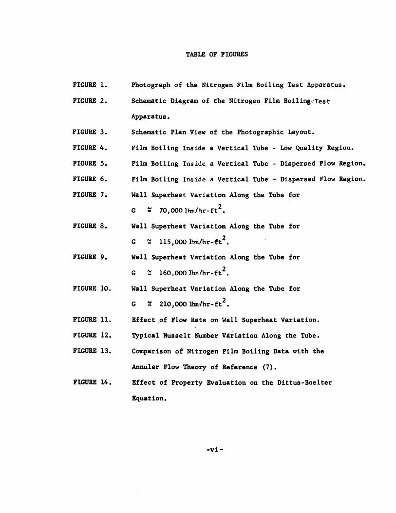
TABLE OF FIGURES

FIGURE 1.

FIGURE 2.

FIGURE 3.

FIGURE 4.

FIGURE 5.

FIGURE 6.

FIGURE 7.

FIGURE 8.

FIGURE 9.

FIGURE 10.

Photograph of the Nitrogen Film Boiling Test Apparatus.

Schematic Diagram of the Nitrogen Film Boiling4Test

Apparatus.

Schematic Plan View of the Photographic Layout.

Film Boiling Inside a Vertical

Film Boiling Inside a Vertical

Film Boiling Inside a Vertical

Wall Superheat Variation Along

G E 70,0001bm/hr-ft2

Wall Superheat Variation Along

G % 115,000 ibm/hr-ft 2 .

Wall Superheat Variation Along

G X 160,0001bm/hr-ft2

Wall Superheat Variation Along

G 2 210,000 lbm/hr-ft 2 .

Tube - Low Quality Region.

Tube - Dispersed Flow Region.

Tube - Dispersed Flow Region.

the Tube for

the Tube for

the Tube for

the Tube for

FIGURE 11.

FIGURE 12.

FIGURE 13.

FIGURE 14.

Effect of Flow Rate on Wall Superheat Variation.

Typical Nusselt Number VAriation Along the Tube.

Comparison of Nitrogen Film Boiling Data with the

Annular Flow Theory of Reference (7).

Effect of Property Evaluation on the Dittus-Boelter

Equation.

-vi -

II

TABLE OF FIGURES (Continued)

FIGURE 15.

FIGURE 16.

FIGURE 17.

FIGURE 18.

FIGURE 19.

FIGURE 20.

FIGURE 21.

FIGURE 22.

FIGURE 23.

FIGURE 24.

FIGURE 25.

Extrapolation of the Experimental Data Toward the

Pure Vapor State; G n 70,000 ibm/hr-ft2

Extrapolation of the Experimental Data Toward the

2Pure Vapor State; G a 210,000 lbm/hr-ft

Calculated Vapor Temperature.

Variation of the Volume Evaporation Coefficient, ahe,

along the Tube.

Droplet Acceleration Analysis.

Calculated Mean Effective Drop Size.

Drop Size Correlation.

Region of Validity of the Dispersed Flow Theory.

Displacement of the Film Boiling Process from an

Equilibrium Condition

Thermal Losses from the Outer Surface of the Test

Section.

Electrical Resistivity of the 304 Stainless Steel

Test Section.

-vii-

II

I. INTRODUCTION

Purpose of the Investigation

The heat transfer process known as film boiling occurs when the

wall confining a liquid is at a temperature much greater than the

saturation temperature of the liquid. When this condition exists

the rate of generation of vapor is so great that a vapor layer, or

film, forms between the wall and the liquid. Once established,

the film acts as a barrier to the flow of heat and allows a large

temperature difference to exist while only a moderate heat flux

passes from wall to liquid. Recent advances in the high temperature

strength of materials and applications of cryogenic fluids as coolants

have created a need for greater understanding of the film boiling

process. Typical examples of the occurance of film boiling are

found in the cooling of rocket engines, the quenching of metals

and in transient temperature fluctuation of liquid cooled magnets

and nuclear reactors upon loss of coolant flow.

As shown in the literature review, previous investigations of

film boiling have been limited to heat transfer from heated surfaces

suspended in a stagnant pool and to forced convection film boiling

where the vapor fraction was small. In view of this, the intent

here is to extend the knowledge of the case of forced convection

film boiling in which large vapor fractions are generated in an

enclosed passage. Previous studies of film boiling at the MIT

Heat Transfer Laboratory have dealt with film boiling at low vapor

fractions of saturated liquid flowing through a uniformly heated tube.

As a result, the extension of the same configuration to include higher

vapor qualities has provided the specific objective: to experimentally

investigate the mechanism of film boiling heat transfer of saturated

liquid flowing upward through a uniformly heated tube for the case

in which most of the liquid is evaporated.

Scope of the Research

Employing liquid nitrogen as a test fluid in tubes heated

electrically by alternating current, two experimental programs were

undertaken. The objective of the first of these was to determine

qualitatively the characteristics of the two-phase flow regimes which

occur as a result of the film boiling process. Using a four foot

long, .417 inch inside diameter pyrex tube, internally coated with

an electrically conducting transparent film, photographs were taken

of the flow regimes along the entire length of the tube for the

the following conditions:

Mass Flow Rate: 75000 lbm/hr-ft2

Heat Flux: = 10000 BTU/hr-ft2

Pressure: - 1.2 atm. absolute

Inlet Temperature: -318 degrees F (saturation temperature)

Inlet Quality: 0

Following these tests a second series was undertaken to determine,

quantitatively, the film boiling heat transfer coefficient. A 304

stainless steel test section having an inside diameter of .319 inches,

an outside diameter of .375 inches and a 47.8 inch length (L/D=150),

was instrumented with thermocouples to measure wall temperature over

the following range of variables:

Mass Flow Rate 70000 to 210,000 lbm/hr-ft2

Heat Flux = 3500 to 30000 BTU/hr-f t2

Wall Temperature = -120 to 650 degrees F

Pressure 1.2 atm absolute

Inlet Temperature " -318 degrees F (saturation temperature)

Inlet Quality = 0

Analysis of the experimental data proceeded to demonstrate the

mechanisms through which heat is carried to the two-phase mixture

and by which evaporation of the liquid takes place. While it had

originally been planned to correlate the data so that the film boiling

heat transfer coefficients could be predicted, the results of the

analysis show that a non-equilibrium condition exists between the

liquid and vapor phases which precludes the success of such a

correlation.

Literature Review

Beginning with the work of Bromley (1)*, dealing with film

boiling in natural convection from a horizontal tube suspended in

saturated liquid, there have been numerous studies of film boiling

*refers to Bibliography at the end of the paper.

from surfaces immersed in pools of liquid with both free and forced

convection. Although Bromley succeeded in drawing an analogy

between film boiling and film condensation such that his boiling

data correlated well using a modified form of the Colburn equation

for film condensation, the later analyses of McFadden and Gross (2)

and of Koh (3) using vertical plates showed that, unlike condensation,

the shear stress at the liquid vapor interface becomes important when

there is any appreciable film velocity.

Aside from the very preliminary work of Carter (4), the subject

of film boiling with forced convection inside of enclosed channels

at low vapor fractions had not entered the literature prior to the

beginning of the current series of film boiling studies at the MIT

Heat Transfer Laboratory. The first of these, the work of R.A.

Kruger (5), dealt with film boiling of saturated liquid flowing through

a uniformly heated horizontal tube. His visual observation of film

boiling of Freon 113 in a transparent, electrically conducting pyrex

tube showed that vapor formed a thin film between the liquid core and

the tube wall in the lower part of the tube and collected by

circumferential flow into a vapor layer at the top of the tube. Using

a model equivalent to the inverse of Bromley's for the thin film

portion, and the Dittus-Boelter single phase, turbulent flow

correlation for the heat transfer to the vapor layer at the top of

the tube, he developed a theory to predict tube wall temperature

distribution which agreed well with his experimental measurements.

Following completion of Kruger's work, an extension of the same

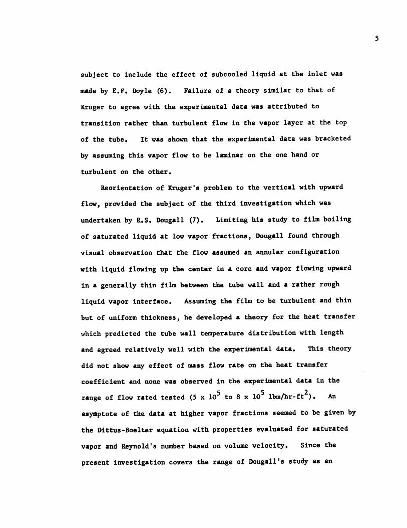
subject to include the effect of subcooled liquid at the inlet was

made by E.F. Doyle (6). Failure of a theory similar to that of

Kruger to agree with the experimental data was attributed to

transition rather than turbulent flow in the vapor layer at the top

of the tube. It was shown that the experimental data was bracketed

by assuming this vapor flow to be laminar on the one hand or

turbulent on the other.

Reorientation of Kruger's problem to the vertical with upward

flow, provided the subject of the third investigation which was

undertaken by R.S. Dougall (7). Limiting his study to film boiling

of saturated liquid at low vapor fractions, Dougall found through

visual observation that the flow assumed an annular configuration

with liquid flowing up the center in a core and vapor flowing upward

in a generally thin film between the tube wall and a rather rough

liquid vapor interface. Assuming the film to be turbulent and thin

but of uniform thickness, he developed a theory for the heat transfer

which predicted the tube wall temperature distribution with length

and agreed relatively well with the experimental data. This theory

did not show any effect of mass flow rate on the heat transfer

coefficient and none was observed in the experimental data in the

range of flow rated tested (5 x 105 to 8 x 105 lbm/hr-ft 2). An

asyAptote of the data at higher vapor fractions seemed to be given by

the Dittus-Boelter equation with properties evaluated for saturated

vapor and Reynold's number based on volume velocity. Since the

present investigation covers the range of Dougall's study as an

initial condition, it was hoped that the above theory would be

substantiated by the new experimental data.

A second correlation developed for film boiling in vertical

tubes is that presented for hydrogen by Hendricks et al (8) which

makes use of the Martinelli two-phase flow parameter in a correction

to the Dittus-Boelter equation. Its agreement with their data was

only approximate and an attempt by Dougall to use it in correlating

his data failed both in magnitude and direction.

The investigation of Lewis et al (9), Parker and Grosh (10),

Lavin and Young (11) and Polomik et al (12) dealt with film boiling

in tubes after a considerable length of nucleate boiling. These

publications contain a wealth of information applicable to the

present problem but perhaps the remarks of Parker and Grosh concerning

the decreased rate of evaporation of droplets once a spheroidal, or

stable film boiling, condition is established are most significant.

The initial length of nucleate boiling is certain to produce a

condition of drops suspended in nearly saturated vapor at the onset

of film boiling whereas an equivalent length of film boiling is likely

to result in considerable vapor superheat since this superheat is

the primary driving force for evaporation in the film boiling process.

Thus the heat transfer coefficients obtained for film boiling at high

vapor fraction with different initial evaporation mechanisms are

likely to differ dramatically.

II. EXPERIMENTAL APPARATUS AND PROCEDURE

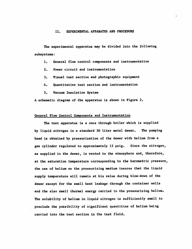
The experimental apparatus may be divided into the following

subsystems:

1. General flow control components and instrumentation

2. Power circuit and instrumentation

3. Visual test section and photographic equipment

4. Quantitative test section and instrumentation

5. Vacuum Insulation System

A schematic diagram of the apparatus is shown in Figure 2.

General Flow Control Components and Instrumentation

The test apparatus is a once through boiler which is supplied

by liquid nitrogen in a standard 50 liter metal dewar. The pumping

head is obtained by pressurization of the dewar with helium from a

gas cylinder regulated to approximately 15 psig. Since the nitrogen,

as supplied in the dewar, is vented to the atmosphere and, therefore,

at the saturation temperature corresponding to the barometric pressure,

the use of helium as the pressurizing medium insures that the liquid

supply temperature will remain at his value during blow-down of the

dewar except for the small heat leakage through the container walls

and the also small thermal energy carried in the pressurizing helium.

The solubility of helium in liquid nitrogen is sufficiently small to

preclude the possibility of signifi'cant quantities of helium being

carried into the test section in the test fluid.

Liquid nitrogen is carried from the bottom of the dewar to the

vacuum chamber which encloses and thermally isolates the test section

and flash cooler, in 3/8 inch OD copper tube which is connected to

the apparatus by a flare fitting. This fitting and the stainless

steel tubes which are sealed to the supply tube on both sides of it,

are insulated by Santocel powder contained by a removable jacket.

This system thus provides an insulated connection which is easily

broken each time the dewar needs refilling.

From the flare fitting, the supply tube passes through a

Swagelok compression fitting which serves as a vacuum seal, into

the vacuum chamber. Inside, the liquid nitrogen is fed to a valve

at which a small part of the stream is bled off to supply the flash

cooler. This cooler is a five foot long, concentric tube, parallel,

flow heat exchanger in which the main nitrogen supply flows in the

center tube and the bleed flow, regulated by the bleed valve, flows

in the annulus between the tubes. Both tubes are type L copper

water tubing, the smaller having a 3/8 inch OD and the larger a 1/2

inch OD. The heat exchanger was coiled to fit in space 34 inches

in diameter by about 14 inches long. From the downstream end of

the cooler, the bleed flow is carried outside the vacuum chamber to

a pressure control valve and then through a steam heater (see pg.ll)

to the intake of a Welch 1397B mechanical vacuum pump. The pressure

in the annulus of the cooler is measured by a bourdon vacuum gauge

connected into the bleed line just upstream of the pressure control

valve.

Following the flash cooler the main nitrogen supply passes

through the flow control valve and through a length of tubing

into the test section. The flow control valve is a Veeco R-38-S

bellows-sealed brass angle valve modified with an extended stem

to permit flow adjustments to be made manually outside the vacuum

chamber. Since the pressure in the test section is only about

2 psig and the nitrogen supply pressure is about 15 psig, the

pressure drop across the flow control valve is sufficient to

prevent small pressure fluctuations in the test section from causing

inlet flow oscillations. The 3 inch long test section inlet tube

is soldered directly into the valve. It is a .375 inch OD, .319

inch ID, 304 stainless steel tube in which 4 static pressure tap is

located at the midpoint and to which is cemented a thermocouple to

measure nitrogen inlet temperature. The pressure tap is connected

to two 24 inch mercury manometers outside the vacuum chaumber, one of

which reads inlet gauge pressure and the other, test section pressure

drop. The helium pressure line is joined through a needle valve

to the connecting tubing of the pressure tap so that air, which

would liquefy in the lines, may be bled out.

On the end of the inlet tubing is silver-soldered a 303 stainless

steel flange having a 1-3/4 inch OD and 4.319 inch ID. This flange

is bolted to a matching flange at the end of the test section with a

1/4 inch thick, 1 inch OD by .319 inch ID micarta spacer between them.

Between each flange and the spacer, a number 17 Viton A 0-ring is

crushed to .015 inches thickness by tightening the six stainless

steel bolts. Since high voltages are applied across the test section,

an interlocking system of micarta spacers is used to provide at least

a 1/4 inch gap between the bolts and the inlet tube and flange at all

points.

At the top of the test section a set of flanges identical to

those at the bottom is used to join the test section to the discharge

tube. Since the discharge tube also serves as the top electrode, no

micarta is used at this connection, only one Viton A 0-ring (crushed

to .015 inches) is required and six brass bolts replace the stainless

steel bolts used at the bottom. The discharge tube, a 1/2 inch OD

type K copper water tube, passes out of the vacuum chamber through

another Swagelok compression fitting seal, makes connection with the

upper power cable and extends into a nylon Swagelok union which

electrically insulates it from the piping downstream. The Swagelok

vacuum seal is connected to the top of the vacuum chamber by a brass

bellows which allows the test section to expand and contract freely.

In order to measure the nitrogen flow rate in a standard rotameter

it is necessary to heat the discharge from the apparatus to near room

temperature. Two independently controlled steam heat exchangers were

put in the flow line for this purpose, one 5 feet long and the other

8 feet long. Between the nylon union and the first heat exchanger,

a second bellows expansion joint was installed to take up thermal

expansion and a second pressure tap was drilled to obtain the test

section pressure drop. Both heat exchangers are tube-in-tube types

made up from type L copper water tubing and sweat fittings. The

inner tube has a 7/8 inch OD and the outer tube a 1-1/8 inch OD.

In both cases the steam passes through the annulus and the nitrogen

through the center tube. The exhaust steam is collected in a single

1/2 inch OD copper tube, passed through the flash cooler bleed line

heater and condensed in a drain line by a stream of water. The flash

cooler bleed line heater is a tube-in-tube heat exchanger in which

the steam exhaust line is the center tube. The outer tube is a 7/8

inch OD copper water tube, 3 feet long, and the bleed flow passes

through the annulus.

Between the second steam heater and the flow meter is a three

foot length of 3/4 inch brass pipe in the middle of which is a

pressure tap connected directly to bourdon pressure gauge. A

thermometer set in a 1/4 inch Conax packing gland is used to measure

gas temperature at the flow meter inlet. The flow meter itself is

a Brooks Model 10-1110 Rotameter calibrated to 1% of full scale

(250 mm = 118 lbm/hr of N2 at 700F and 14.7 psia). Following the

flow meter the nitrogen passes through a pressure control valve and

is exhausted to the atmosphere.

Power Circuit and Instrumentation

The 115 volt, 60 cycle alternating current laboratory power

is used as the power source for heating the test section. It has

a 3kw capability, sufficient to produce a bulk quality of 1.0 at

the test section exit (saturated liquid at the inlet) over the

entire range of flow rates studied. A 5 KVA Variac variable

transformer which can convert the 115 volt supply to from 0 to 135

volts, is used to control the test section power. Since the visual

test section has an electrical resistance of approximately 380 ohms

while the quantitative test section has a resistance of only about

.04 ohms, two different transformers were required to convert the

Variac output to voltages compatible with the test section resistance

and power dissipation requirements. The transformer used with the

visual test section is a Westinghouse Type CSP single phase transformer

having a 7.5 KVA rating and wired to boost the input voltage by a

factor of 10. The one used with the quantitative test section is a

GE Boost and Buck transformer Model 9T51Y113 which has a rating of

3 KVA and was wired to reduce the input voltage by a factor of 10.

The power input to the test section, in both cases, was measured

by current and voltage readings from a-c meters. For the visual test

section, a Model 59 Simpson voltmeter with external multiplier giving

it a range of 0 to 1000 volts and a Model 59 Simpson ammeter with a

range of 0 to 3 amps were used. Since the current was small and

line losses were negligible for the visual set up, the voltmeter

was located with the ammeter on the high voltage transformer enclosure

and the voltage taps were made close to the transformer. The meters

used with the quantitative test section were a Model 115 Weston ammeter

with a range of 0 to 250 amps and a Model 433 Weston voltmeter with

a 0 to 10 volts, O to 20 volts dual range. Both of these latter

instruments were calibrated to give t 1/2% of full scale accuracy.

Since the line losses were appreciable, the voltmeter taps were made

at the discharge tube at the top of the vacuum chamber and at the

external end of the Conax electrode gland.

Two different sets of power cables-were used to carry the

power to the apparatus for the two test sections. The cables

used for the visual test section are No. 14, 15 KV rated wire

while those used for the quantitative test section are 3/0 welding

cable. The connection at the top of the test section was made by

connecting the cable to a brass clamp which is bolted tightly around

the nitrogen discharge tube. At the lower end a Conax electrode

gland, No. EG-31-Cu-L type A, was employed to carry the power inside

the vacuum chamber. When used with the high voltage power supply,

the exposed end connections of the gland were covered completely

with electrical tape as a safety precaution. Inside the chamber

two different arrangements were used to connect the gland to the

lower flange of the test section. For the visual test section it

was sufficient to simply run a short length of high voltage wire

from the gland to one of the stainless steel flange bolts, using

an extra nut to faster it in place. For the quantitative test

section a 1 inch by 1/16 inch copper strip was used to connect the

gland to a 1/8 inch thick, U-shaped plate which was bolted down

against the flange nuts by six additional nuts. In order to

measure the heat conduction loss through the buss, two thermocouples

were attached to the copper strip 1 inch apart. The outer one was

wired to read the buss temperature and the inner one was wired to

read the temperature difference between them.

Visual Test Section and Photographic Equipment

As mentioned previously the visual test section is a pyrex tube

internally coated with a transparent electrically conducting coating.

It has a .512 inch OD and a .417 inch ID and is joined to end flanges

by graded glass, pyrex to kovar, seals and 1 inch lengths of kovar

tubing copper-gold sol4ered to the flanges. The E-C coating which

forms a 45.9 inch heated length was applied by the Corning Glass

Works on an experimental basis. A layer of diIver fired onto the

tube makes the electrical contact between the coating and the end

flanges. Since the coating is limited to a maximum operating

temperature of 6600F, one thermocouple was attached to the outside

of the tube about six inches from the test section to monitor tube

temperature. Thermal isolation of the test section, except for

small end losses and radiation losses, was provided by vacuum

insulation as is discussed more fully on page 16. In order to see

the test section and make visual studies, the portion of the vacuum

chamber surrounding the test section was made from a transparent

lucite tube.

Flow regime photographs were taken with a Polaroid Model 110B

camera using close-up lens' which give a 3 inch by 4 inch field at

a focal distance of 6 inches. The film used was Polaroid Type 47

(ASA 3000) and the lighting was provided by a General Radio Type

1530-A Microflash which was tripped by the camera shutter. For easy

adjustment of camera position anywhere along the test section, a

tubular "unipod" was built along which a camera support arm can be

slid and clamped to give the desired field.

Quantitative Test Section and Instrumentation

The quantitative test section is a .375 inch OD, .319 inch ID

304 stainless steel seamless tube which is 47.8 inches long. At

each end a 303 stainless steel flange is silver soldered to it for

connection with the inlet and discharge piping (see page 9). Fifteen

copper-constantan thermocouples are cemented with magnet wire varnish

to its external surface at approximately 3 inch intervals (see Table I).

These thermocouples were made up from 30 gauge glass wrapped duplex

wire and were calibrated over the range of operating temperatures.

A thin (.002 inch) piece of mica is imbedded in the cement under the

bare end of each thermocouple junction in order to electrically insulate

it from the test section. In addition, approximately the last inch of

wire before each junction is cemented to the tube wall to provide a

heat sink for the lead wire without inducing thermocouple errors. An

aluminum foil radiation shield, separated from the tube by a layer

of asbestos cloth tape and cut to fit around the thermocouple lead

wires, is wrapped around the test section to reduce the radiation loss

from the test section and thermocouple junctions. This entire unit is

enclosed in the vacuum chamber to eliminate convection losses to the

surroundings.

ml

The constantan wires from the fifteen test section thermocouples,

the inlet tube thermocouple and the buss bar temperature thermocouple

were soldered together inside the vacuum chamber and one 24 gauge

constantan wire was run from this junction through a pass-through

tube to an ice junction outside the vacuum chamber. Each of the

copper wires from the above thermocouples plus the one from the

temperature difference thermocouple on the buss bar was run through

its own pass through tube to the outside. The fifteen test section

thermocouples and the inlet temperature thermocouple were then wired

up so that they could either be read on a 16 channel Brown recorder

(Minneapolis-Honeywell Model 153X62V16) or by a potentiometer or

millivoltmeter. The two buss bar thermocouples were wired to be

read on the potentiometer or millivoltmeter only. The recorder has

a range of 0 to 10 millivolts and was wired so that negative potentials

could be read simply by flipping a switch. For the few runs in which

wall temperatures occurred which produced thermocouple emf's greater

than 10 millivolts, a constant measured emf was added into the circuit

to convert the recorder range to slightly higher values (e.g. 5 to 15 mv).

Vacuum Insulation System

The vacuum chamber consists of two sections. The lower section

which contains the flash cooler and flow control valve, is a 5 inch

OD brass tube, 18 inches long with 1/2 inch thick brass end plates.

Through the bottom plate which is soldered to the brass tube, pass

the enclosed flow control valve stem, sealed by a neoprene O-ring

and the nitrogen supply tube, sealed by a Swagelok compression fitting

at the bottom end of a six inch stainless steel extension tube. The

top plate is bolted to a flange on the brass tube and sealed by a

neoprene 0-ring. The bleed flow line and enclosed bleed valve stem

pass through the top plate and are sealed by Swagelok compression

fittings. The Conax electrode gland is also located in this plate

as is the miniature Conax packing gland which seals the tube for the

inlet flow pressure tap. A 1-3/8 inch OD copper tube which is silver

soldered into the brass tube just below the flange, serves as the

evacuation port for the vacuum chamber. It is connected through a

1 inch diaphagm valve and a liquid nitrogen cold trap to a second

1397B Welsh mechanical vacuum pump. On either side of the evacuation

port are two electrical pass-throughs, each of which consists of 6

or 9 small electrically insulated vacuum tight tubes for thermocouple

wires to pass through and be soldered to.

The upper section of the vacuum chamber is a four foot long,

3 inch OD, 2-1/2 inch ID lucite tube which is sealed at each end

by neoprene 0-rings. It is held between the top plate of the lower

chamber and a 1/2 inch thick brass cover plate by four 1/4 inch

diameter stainless steel rods. These rods are spring loaded at the

top to permit thermal expansion of the lucite. Since the cover plate

is in electrical contact with the top power cable it was necessary

to. insulate it from the lower section of the vacuum chamber. This

was accomplished by wrapping each of the rods with several layers of

electrical tape in the region where they pass through the cover

plate and by placing micarta washers under the springs.

Vacuum chamber pressure is sensed by -a National Research

Corporation Type 501 Thermocouple Gauge located in the evacuation

line near the lower chamber. The control unit for the gauge is

an NRC Type 701.

Experimental Procedure

Before hooking up a full dewar of liquid nitrogen the vacuum

chamber is evacuated to a pressure of about 1 micron of mercury

absolute and the entire flow system is flushed with prepurified

nitrogen from a gas cylinder. With the dewar in place and pressurized

and the steam heaters turned on, the apparatus is ready to operate.

The first steam heater is set initially and then not changed since

it is in danger of freezing up at low steam flow rates. Cool-down

of the inlet piping proceeds by opening the flow control valve while

at the same time adjusting the test section power to keep the test

section wall temperature in the film boiling range. When the inlet

temperature approaches saturation temperature, the bleed valve is

cracked open to start the cold stream through the flash cooler.

After the inlet flow reaches the pure liquid condition, -the flow

control valve, and back-pressure control valve are set to give the

desired flow rate and system pressure, and the variac and second steam

heater are set to give the desired test section heat flux and flow

meter inlet temperature. A small amount of helium is then bled

into the lower pressure tap tube to purge the air from it and the

system is ready for operation.

Although no provision was made for measuring the bleed flow

rate and the copper constantan inlet temperature thermocouple is

not sufficiently accurate to measure inlet subcooling, the operating

procedure for the bleed system was easily established during visual

testing by observing the bleed control settings at which vapor is

just eliminated from the inlet flow. Since the heat flow into the

dewar and lower chamber is independent of flow rate and test section

heat flux, one setting was obtained which could be used throughout

the testing. The bleed back-pressure valve was then left in this

position and the bleed flow control valve was set each time to give

a back-pressure of about 22 inches of mercury vacuum at the gauge.

This resulted in a flash cooler cold stream temperature of about

120 0 R and a nearly constant bleed flow rate.

For each visual run the following quantities were recorded:

flow rate-mm, flow meter temperature-OF, system back pressure-psig,

test section current-amps and voltage-volts, inlet flow temperature-

my, test section reference temperature-mv, bleed pressure-inches

Hg vacuum and photograph numbers and positions. Preliminary testing

proved that backlighting, obtained by bouncing the Microflash light

off a white background, was most effective in illuminating the flow

patterns while avoiding reflections from the lucite and pyrex surfaces.

At high vapor qualities, a white background with a black center

directly behind the portion of the tube being photographed, was found

to provide the better contrast needed to outline very small droplets.

Figure 3 is a schematic plan view of photographic layout.

The quantitative data was taken for a range of heat fluxes at

each of four flow rates, G ^= 70000, 115000, 160000, 210000 lbm/hr-ft2

The Brown recorder, which cycles through the 16 channels about once

every 20 seconds, was used both to record the tube wall and inlet

temperature and to establish when a run had reached equilibrium

conditions. On the average it took about 10 minutes for a run to

reach equilibrium and, as a result, from four to eight runs could

be made on one 50 liter charge of nitrogen depending on the flow rate.

Once the system reached equilibrium the following quantities were

recorded manually: flow rate-mm, flow meter temperature- F, system

back-pressure-psig, test section current-amps, and voltage-volts,

test section inlet pressure and pressure drop-mmHg, bleed pressure-

inches Hg vacuum, and lower buss temperature and temperature

difference-mv. Two series of data runs were made in order to

establish reproducibility.

III. DATA ANALYSIS, RESULTS AND DISCUSSION

Reduction of Experimental Data

For both the visual and quantitative tests the flow rate data

was reduced to lbm/hr with the rotameter calibration curve and

temperature and pressure correction curves. Flow meter inlet

temperature and system back-pressure corrected to absolute pressure

were used to evaluate the temperature and pressure correction

factors respectively.

Since the visual studies were intended to be only qualitative

in scope and the heat flux was relatively non-uniform, the average

heat flux in BTU/hr-ft2 was estimated using the equation:

A T I EJLo

and the local vapor quality was estimated by the equation:

I L (2)A G hg ~D W

where h was evaluated at the system back pressure.

The average heat flux for each of the quantitative test runs

was computed using the equation:

9- I-.IE-TR (3)

uss was estimated by the equation:

R6A5 97.1 "n.' r(T~s ) + I k [)..L (4)

where the first term is the resistance of the lower buss between

the lower voltage tap and the lower test section flange and the second

term is the resistance of the discharge tube between the upper voltage

tap and the upper test section flange. The 12 R buss term was less

than 0.3% of the IE product for all runs. Qloss, the thermal loss

from the outer surface of the test section, was taken from Figure 24

at the average test section wall temperature. It was less than 1.8%

of the IE product for all runs. The thermal loss data for Figure 30

was obtained from no flow tests using the equation:

,- (w-rs Cp- + WI 7(5)L~oss T3 PPZe , s

where Wrs Crr is the heat capacity of the test section and

Wr C-r is the heat capacity of the asbestos 'insulation between

the test section and the radiation shield.

Test section inlet pressure, P , was converted to absolute

pressure in psia using the barometric pressure, and test section

pressure drop, 6P, was converted to psi. The pressure drop was

found to be sufficiently small 'that the heat of vaporization, h ,

varied no more than 1% in the length of the test section.

Therefore h was always evaluated at Pg .

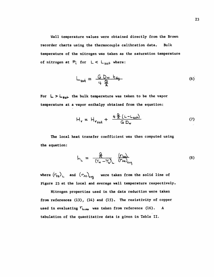
Wall temperature values were obtained directly from the Brown

recorder charts using the thermocouple calibration data. Bulk

temperature of the nitrogen was taken as the saturation temperature

of nitrogen at PL for L < L s.+ where:

L h (6)42.

For L > L.,,.. the bulk temperature was taken to be the vapor

temperature at a vapor enthalpy obtained from the equation:

H + 4 7(7)V Hvsat G DW

The local heat transfer coefficient was then computed using

the equation:

ssL ' (8)' (TW -TX (I'ss

where (rsa)L and were taken from the solid line of

Figure 25 at the local and average wall temperature respectively.

Nitrogen properties used in the data reduction were taken

from references (13), (14) and (15). The resistivity of copper

used in evaluating r~a, was taken from reference (16). A

tabulation of the quantitative data is given in Table II,

Visual Study

From the visual study it was determined that there are basically

two flow regimes which occur. At the beginning of the heated section,

where the vapor fraction is small, the flow is annular with the liquid

in the center and the vapor in the annulus as shown by Figure 4a.

Because of the large velocity increase caused by the generation of

low density vapor, the drag force on the liquid core increases at

greater tube lengths to the point that the core is torn apart into

filaments and droplets of liquid. The beginning of this break-up is

evident at the top of Figure 4b. As the break-up continues the flow

goes through a somewhat gradual transition to a dispersed flow regime

in which small droplets and filaments of liquid are carried along in

a vapor matrix. Figures 5 and 6 illustrate the nature of the dispersed

flow. In Figure 5 the decrease of average drop size with increasing

length (and vapor quality) and a tendency of the largest liquid particles

to be concentrated in the vapor boundary layer are both evident. Also

noticeable in the progression from 5a to 5b is the characteristic of

the particles to become more uniformly distributed at greater vapor

qualities. Figure 6, taken with the dark background which tends to

bring out the very small droplets at the sacrifice of obscuring the

larger ones, is a duplicate of the conditions of Figure 5a. The two

photographs were taken a few seconds apart and show the unsteady nature

of the flow of the very small drops. This effect was easily seen by

the naked eye and is apparently due to periodic shattering of large

liquid filaments in a region about ten inches from the start of the

heated section.

Quantitative Study

Figures 7 to 11 summarize the results of the quantitative

experimental program, showing wall superheat variation with heated

length, heat flux and flow rate. For the lower flow rates the wall

temperature rises from the inlet to a maximum value after which it

decreases smoothly to a minimum. Both the maximum and the minimum

are seen to move away from the inlet as heat flux is decreased and

as flow rate is increased. By comparison of the visual results

with the data of run 26 (Figure 7) which has approximately the same

heat flux and mass velocity as that used in the visual tests, it was

found that the maximum wall temperature corresponds to the transition

to dispersed flow. Since both the vapor fraction and fluid

acceleration at a given length decrease with decreasing heat flux

or increasing mass velocity, the transition must at least shift in

the same direction as does the temperature maximum. The secondary

depression of wall temperature following the maximum for the highest

level of flow rate (Figure 10) is not accountable but it is suggested

that the initial breakup of the liquid core may occur suddenly at a

critical liquid-vapor velocity difference or Weber number after which

dispersion continues in the gradual manner found in the visual study.

In order to present the data in a more conventional form, the

local heat transfer coefficients for typical runs at each flow rate,

converted to Nusselt number, , . are shown in Figure 12.

Although data points are not plotted for the sake of clarity the

scatter from each line was no more than three percent. In Figure 13 some of

these data are compared with the theory of Dougall (7). Since his

experimental results showed no significant effect of either heat

flux or flow rate upon Nusselt number in the low quality range

there is no agreement between his theory and the nitrogen data.

The most apparent cause of the discrepancy lies in the assumption

used in the theory that the vapor annulus remains thin relative to

the tube diameter. From the visual results it is quite evident that

this is not the case in film boiling of liquid nitrogen. Why it

should be valid for Freon 113 when it is not for nitrogen remains

as yet an open question.

In order to understand the behavior of the wall temperature at

higher vapor qualities it is well to consider the asymptote which is

met when the evaporation is complete. If equilibrium were maintained

between the two phases, this would occur at a length, Lsa. , given

by equation (6). Since over the range of flow rates studied the

pure vapor state implies turbulent flow, we should be able to predict

the wall temperature for L > L. using a form of the Dittus-Boelter

equation:

__-D o Wj Pr c. (9)

For a high wall-to-fluid temperature ratio it has been suggested

(e.g. ref. 17) that the fluid properties be evaluated at film

temperature, Tg = -L (T + T6), and that the veloc ity used in

computing the Reynolds number be evaluated at the bulk temperature

so that the equation becomes:

h -V. V - wf P r 4. (10)

Figure 14 is a comparison of wall temperatures of run 56 with those

calculated by equations (9) and (10) assuming saturated vapor at

length Lsa. and the heat flux and mass velocity of run 56. The

high values of wall temperature predicted by equation (10) at low

vapor superheats is due to the rapid percentage increase of nitrogen

vapor density, with corresponding decrease in bulk velocity, as

saturation is approached. In the region in which equation (10) has

been tested (e.g. ref. 18) the absolute temperature of the gas was

much greater than that of saturated nitrogen and the correction

resulting from the difference between equations (9) and (10) was only

a shift of wall temperature level and not a change of curve shape.

Since there is no known available data for heat transfer to cryogenic

vapors in turbulent flow to confirm such a large temperature ratio

effect as that given by equation (10), it was decided that equation (9)

provides a better estimate of the heat transfer coefficient for nearly

saturated nitrogen vapor.

Two Step Heat Transfer Theory

Using equation (9) to compute the pure vapor asymptotes Figures

15 and 16 show the results f several runs at the lowest and highest

flow rates with extrapolations showing approximately how they would

approach their respective asymptotes if the heated test section were

sufficiently long. On each run is indicated the point L at, at

which the pure vapor state would have been attained had the vapor

been in thermal equilibrium with the liquid (i.e. for Tv=T sat.

The fact that the data does not meet the asymptote at this length

shows that a significant amount of superheat is present in the vapor

and that the film boiling is not an equilibrium process. Therefore,

as a model for the high quality, dispersed flow region of film

boiling, it seems reasonable to assume that the heat transfer process

may take place in two steps; first, from the wall to vapor at some

temperature Tv, and second, from the vapor to the liquid. Since this

implies that most all of the evaporation occurs outside the vapor

boundary layer, the model will obviously be invalid for low qualities

where the visual studies show there is a concentration of large liquid

drops near the wall.

Heat Transfer to the Vapor

For the first step, assuming the vapor flow to be turbulent,

the heat transfer may be calculated from a revised form of equation

(9):

~ - 8 o.'4

.E % F 1

where the term L ,v + 9f is the through-put velocity and is

At.calculated using the equation

cL*% _ 4 . L 0Dv -v L fH 'so GA t (H -I-I ) \(12)

For the wall temperatures involved in the region of interest, the

radiation emitted by the wall9 assuming the wall to be black,

amounts to no more than 5 percent of the total heat flux. Since

the flow is dispersed, much of that energy strikes the tube wall

elsewhere and is absorbed, Therefore radiation to the liquid is

negligible and it follows that;

_r Qw r(13)

The local heat flow for the second step is related to the

first step by the heat balance:

£ P A 8 L(14)

II

where is the heat going into evaporation per unit volume of liquid-

vapor mixture and WV, the vapor flow rate is calculated using the heat

balance:

H- A

Defining a volume evaporation coefficient, cte_ - - v

equations (14) and (15) become:

ak_ = IQ -QOP (16)Tv-T D A Hv-H dL / (

where h_ is the mean evaporation heat transfer coefficient and ae

is the liquid surface area per unit volume of liquid-vapor mixture.

Limits of the Theory

Before proceeding with an analysis of the evaporation process

of the second step, a check of the region of application of the

theory is possible by computation of ah from the experimental data.

When equations (11), (12) and (13) have been combined to form the

equation:

A k - t4L ()V23T A -,T -vI((17)Tw T * ' 9 .v rf (Hv4 - Hg) \ (17) 9

it is evident that the vapor temperature can be found for each run

at any length, L, simply by iteration. Figure 17 shows the calculated

vapor temperature for a few typical runs. From plots like Figure 17,

the slope, , was measured at various values of L and equation (16)

was solved for ahe. Figure 18 shows the variation of ahe with heated

length for a portion of the test runs at each of the four flow rates.

The left end of each line corresponds to a calculated vapor superheat

of 200F. The rapid increase of ah at this end of the line indicates

that significant amounts of liquid are in the boundary layer and,

therefore, that the theory is invalid in this region. The figure

shows that ah increases for higher mass velocities, increases slightly

for higher heat fluxes and decreases slightly with length. For

those runs which reached the highest vapor qualities it may be seen

that ah starts to drop more rapidly near the end of the heated test

section. The most plausible explanation of this slope change is that

it marks the end of drop breakup and thus the end of a process which

increases a. As a final remark about Figure 18 it seems well to

point out that ah must go to zero when the evaporation is complete

since a must then be zero.

Evaporation of the Liquid

Both a and h depend on fluid properties, slip velocity and

drop size. Because of the extremely complex nature of the breakup

of the annular flow, the drop size spectrum is not something which

can be predicted by analysis of the fluid mechanics. Neither is

it possible to experimentally measure the drop size, except as an

order of magnitude estimate. For this reason, it is necessary to

complete the analysis without the knowledge of drop size and to use

the experimental data to provide the missing information.

Assuming that each drop is a sphere and knowing that the Prandtl

number of nitrogen is about the same as air, the mean heat transfer

coefficient, h,, can be gotten from the following equation from

McAdams (17):

he Dd vi VL U (8)7 (18)

as long as the drop Reynolds number , is greater than 17.

Integrating over all drop sizes, a is given by the equation:

c = r W d D (19)0

where N is the concentration function for drop diameter. Similarly,

the equation:

oo

0 3 ( NIdD (20)

is obtained by integrating the mass of all the drops contained in a

unit volume of liquid-vapor mixture.

If the assumption is now made, that there is one equivalent

drop diameter, Ds, which, when substituted for the real drop spectrum,

will give the same resulting heat transfer, Dd can be replaced by Ds

in equations (18), (19) and (20) with the result:

0..6

la bs -\ AV (18a)

CL 9n~

A -n() (20a)

Combining these last three equations and solving for ahe produces

the equation:

_L (21)

which gives the effective evaporation heat transfer coefficient in

terms of the mechanics of the evaporation process. By expressing

the liquid flow rate as the total less the vapor flow and the liquid

velocity as the vapor velocity less the slip velocity, equation (21)

is reduced to the form:

C) o' Gr

kI &vV~s04,G (22)

VI

Since vapor velocity can be estimated in the quality range of interest

by the equation:

-.(23)v ~ v A, ~ v _w ( (Hv - Ht)(3

the only variables left in equation (19) are drop size and slip

velocity. By writing a force balance on a single drop of diameter

D S)the slip velocity is obtained in the form:

s . A (24)

which upon reduction yields:

6 / Z L + a (25)

Although equation (25) is not in closed form because of the

presence of the derivative, , a first estimate of AV may be

made by assuming that d L) is small so that = . Figure 194 L dL 4L

shows the results of such an assumption for two different sized drops

exposed to the conditions of run 53. The variation of drop diameter

with length was estimated, assuming that (QeYrr =

by the equation:

D LL

e L (_v-Ng d L (26)

For the small drop, D = .1mm, it was found the assumption

was adequate while for the larger drop, D = 1mm, it was found

that a better assumption was 8L . Since the solution

of equation (25) implies an initial slip velocity, equation (24)

was solved by finite difference techniques to determine the effect

of greater values of AV at L . The dashed lines of Figure 19

show the results of these calculations and indicate that the use of

equation (25) to calculate slip velocity is a valid procedure.

Mean Effective Drop Size

By the simultaneous solution of equations'(22) and (25) it is

now possible to calculate a mean effective drop size at various lengths

for any of the experimental runs. Figure 20 shows the results of

these calculations for runs covering the entire flow rate, heat flux

range of the experimental program. In solving equation (25)a drag

coefficient of .5 and linear interpolation of A with drop size

between at D = .1mm and .(, at 1mm,1i L d L s 5L

were found to be adequate for all cases. The drop diameters shown in

Figure 20 are all less than 1mm as would be expected from the visual

studies. In the calculated drop sizes for runs 3 and 53, the rate

of decrease of drop size with increasing quality is seen to decrease

at higher quality corresponding to the end of drop break-up. At the

lowest quality value shown for runs 31 to 51, the calculated drop

size decreases because of the ah increase created by breakdown of

the two step theory. As would be expected from the mechanics

of the break-up process, higher heat fluxes, with the attendant

increase in vapor acceleration, give smaller drop sizes at the same

quality while higher flow rates which need greater tube lengths to

produce the same quality, also produce smaller drop sizes.

In Figure 21 a correlation of the drop size data is shown for

the range of the two step theory in which break-up of drops is present.

Since no check of the correlation to determine the effect of fluid

properties or tube diameter is possible within the scope of this

work, it is presented without assurance that it is applicable over

a broader range of variables than those encompassed herein.

Because of the sensitivity of equation (16) to notonly vapor

temperature but also Sr the use of the drop size correlationdL-

to predict wall temperatures and overall heat transfer coefficients

for film boiling is not possible. However, in spite of the failure

of the theory to produce a useable heat transfer correlation, much

has been learned about the mechanics of the film boiling process

through the success of the drop size calculations. Most important,

it has been confirmed that a two step process will work. Therefore,

if the local vapor temperature is known, the wall temperature and heat

transfer coefficient may be calculated simply by use of equations (17)

and (13) respectively, as long as the basic assumption of inlet

conditions, uniform heat flux and dispersed flow are met, As a

guide to determine the minimum quality for which the dispersed

flow condition is met, Figure 22 shows the limits of the theory found

for the experimental range covered in this program. Although the

vapor temperature will be unknown in most cases, an upper bound on the

heat transfer coefficient will be obtained from the equations by assuming

that the vapor is at saturation temperature. Since this implies

equilibrium between the phases, the corresponding upper bound of quality

is given by the equation:

X=L (27)

In Figure 23 the actual quality for typical experimental runs,

calculated by dividing equation (15) by the total flow rate, is

compared with the equilibrium condition of equation (27). The

departure of the data from the equilibrium condition is related to

local vapor temperature through the equation:

H, = H, + 4 _%- L (28)

Therefore, if it is desired to make an estimate of the film boiling

heat transfer coefficient which is better than the upper bound

presented above, the value of vapor temperature may be obtained

using Figure 23 in conjunction with equation (28). In making

this suggestion it seems well to point out that the displacement

of the data from the equilibrium condition is dependent upon the

mechanics of the evaporation process. Consequently, it would be

expected that increased heat flux and incteased mass flow rate would

move the process toward the equilibrium condition and that decreases

of these variables would move it away. In addition, variation of

fluid properties would undoubtedly have a strong effect while tube

diameter effects might well be accounted for by using volume heat

flux A ?in correlating heat flux effects.

Conclusion

In conclusion, the results obtained from the analysis are

summarized as follows:

1. For film boiling of saturated liquid flowing upward through

a uniformly heated vertical tube, there are two basic flow regimes:

near the inlet the flow is annular with liquid in the core and vapor

in the annulus; at higher vapor fractions the core is broken up

to give a dispersed flow regime in which droplets and filaments are

carried along in a vapor matrix.

2. In the case of nitrogen, the thickness of the vapor annulus

grows very rapidly so the theory derived by Dougall (7), for film

boiling at small vapor fractions, does not agree with the experimental

results obtained with nitrogen.

3. In most cases the break-up of annular flow is gradual and

tube wall temperature reaches a simple maximum in the vicinity of the

transition but at mass velocities greater than about 180,000 lbm/hr-ft 2

with high heat fluxes, there is a depression of wall temperature following

the maximum which indicates that a critical Weber number may be involved

at which the break-up begins suddenly.

4. Once transition has proceeded to the degree that drops are

relatively uniformly dispersed, the heat transfer may be considered to

be a two step process in which 1) all of the heat from the wall is

transferred to the vapor and 2) heat is transferred from the vapor to

the liquid.

a. The heat transfer coefficient between the wall and the

vapor is given approximately by the equation:

_ _ - ._Z ( (11

b. Evaporation rate of the liquid is controlled by drop

size, vapor velocity and acceleration, and vapor temperature.

c. Because the evaporation heat transfer coefficient is

not large compared to the wall-to-vapor coefficient, a significant

amount of vapor superheat is present and it is impossible to obtain

40

a simple expression for the overall heat transfer coefficient.

d. Use of Figures 22 and 23 together with equations (13)

and (17) provides a method by which both an upper bound and an

approximation for the actual heat transfer coefficient can be obtained

in the region of validity of the theory.

NOMENCLATURE

a Surface area of drops per unit volume of liquid-vapor mixture

Ac Cross sectional area for fluid flow through the test section

CD Drag coefficient

Cp Specific heat

Dd Drop diameter

Ds Equivalent mean drop diameter for the evaporation process

D Inside diameter of the test sectionw

E Voltage drop across the test section

G Mass velocity,

g Gravitational acceleration

h Overall heat transfer coefficient at any location along the

test section

h Local heat transfer coefficient between the wall and the vapor

h Evaporation heat transfer coefficient

h Latent heat

H Enthalpy

I Electric current passing through the walls of the test section

Jgo Mechanical equivalent of heat conversion factor

k Thermal conductivity

L Distance from the start of the test section

L Total length of the test section

Lsat Length to complete evaporation in an equilibrium process

m Mass

N Concentration of drops of a given sized 412d4Dd

NOMENCLATURE (Continued)

n Number of drops per unit volume of liquid-vapor mixture

P Pressure at the test section inlet

AP Pressure drop across the test section

Pr Prandtl number,

Heat flux from the walls of the test sectionA

Qloss Total thermal loss from the outer surface of the test section

Q Heat going into evaporation

__ Heat going into evaporation per unit volume of liquid-vapor

mixture

q Average volume flow rate of liquid at any location along the

test section

qv Average volume flow rate of vapor at any location along the test

section

R Electrical resistance

r Electrical resistivity

T Average temperature of the vapor boundary layer at the wall,

4(T +Tv)

T. Average temperature of the vapor at the evaporation interface1.

on a drop of liquid k(T +T )v s

Tv Vapor temperature

T Wall temperature (on the inside surface of the test section)

T wo Temperature on the outside surface of the test section

Vd Drop velocity

NOMENCLATURE (Continued)

V Liquid drop velocity

AV Slip velocity, Vy -V e

WV Mass flow rate of vapor

W1 Mass flow rate of liquid

L'Ot Total mass flow rate

X Quality,)V

Wall thickness of the 304 stainless steel test section

Viscosity

Surface tension

Density

Subscripts

b Quantities evaluated at bulk temperature (see eqn. 7)

buss Refers to copper buss bars connecting the test section to

the power cables

eq Quantities evaluated assuming an equilibrium process

f Quantities evaluated at film temperature, Tf

i Quantities evaluated at interface temperature, Ti

L Quantities evaluated at a length L

I Quantities evaluated for saturated liquid

sat Saturation

ss Quantities refering to stainless steel test section

v Quantities evaluated for vapor at TV or at some other

temperature if specified by a second subscript.

BIBLIOGRAPHY

1. Bromley, L.A."Heat Transfer in Film Boiling"Chemical Engineering Progress, Vol. 46, 1950, P. 221.

2. McFadden, P.W., and Grosh, R.J."High-Flux Heat Transfer Studies: An Analytical Investigationof Laminar Film Boiling"AEC Research and Development Report, ANL-6060, 1959.

3. Koh, J.C.Y."Analysis of Film Boiling on Vertical Surfaces"ASME Paper No. 61-SA-31.

4. Carter, J.C."The Effect of Film Boiling"AEC Research and Development Report, ANL-6291, 1961.

5. Kruger, R.A."Film Boiling on the Inside of Horizontal Tubes in ForcedConvection"M.I.T. Ph.D. Thesis, June, 1961.

6. Doyle, E.F."Effect of Subcooling on Film Boiling in a Horizontal Tube"S.M. Thesis, M.I.T.,June, 1962.

7. Dougall, R.S."Film Boiling on the Inside of Vertical Tubes with Upward Flowof the Fluid at Low Qualities"M.I.T., Department of Mechanical Engineering, EPL Report No. 9079-26.

8. Hendricks, R.C., Graham, R.W., Hsu, Y.Y., and Friedman, R."Experimental Heat Transfer and Pressure Drop of Liquid HydrogenThrough a Heated Tube"NASA TN D-765, May, 1961.

9. Lewis, J.P., Goodykoontz, J.H., and Kline, J.F."Boiling Heat Transfer to Liquid Hydrogen and Nitrogen in Forced Flow"NASA TN D-1314, Sept., 1962.

10. Parker, J.D., and Grosh, R.J."Heat Transfer to a Mist Flow"AEC Research and Development Report, ANL-6291, 1961.

BIBLIOGRAPHY (Continued)

11. Lavin, J.G. and Young, E.H.'Heat Transfer to Evaporating Refrigerants in Two-Phase Flow"Preprint 21e AIChE Fifty Second Annual Meeting, Memphis, Tenn.,February 1964.

12. Polomik, E.E., Levy, S., and Sawochka, S.G."Film Boiling of Steam-Water Mixtures in Annular Flow at 800,1100, and 1400 Psi"ASME Paper No. 62-WA-136.

13. Scott, R.B.Cryogenic Engineering D. Van Nostrand Co., Inc., Princeton,N.J., 1959.

14. Chelton, D.B. and Mann, D.B."Cryogenic Data Book"U.S. Air Force, WADC Technical Report 59-8, 1959.

15. Strobridge, T.R.'The Thermodynamic Properties of Nitrogen from 64 to 300 KBetween 0.1 and 200 Atmospheres" NBS TN 129, January 1962.

16. Handbook of Chemistry and PhysicsChemical Rubber Publishing Co.,Forty-Third Edition, 1961-1962.

17. McAdams, W.H.Heat TransmissionMcGrall-Hill Book Co., Inc.New York, 1954.

18. Humble, L.V., Lowdermilk, W.H., and Desmon, L.G."Measurements of Average Heat-Transfer and Friction Coefficientsfor Subsonic Flow of Air in Smooth Tubes at High Surface and FluidTemperatures"NACA Report 1020, 1951.

APPENDIX A

DISCUSSION OF ERRORS

The experimental errors were of three types: those due to

instrumentation accuracy and sensitivity, those caused by system

losses and those caused by system instabilities. It is useful

to discuss separately errors in the four measured items: flow,

heat flux, pressure and temperature.

The errors in flow measurement were due to lack of sensivitiy

of the rotameter and to system instabilities. The rotameter was

calibrated for + 1% of full scale accuracy which gives an absolute

error of + 1.2 lbm/hr. Therefore the reading accuracy of flow

rate varies from + 3.1% at the lowest flow rate to + 1% at the

highest flow rate. Because the system is a once through boiler

there are inherent instabilities. For a flow of the runs flow

oscillations occurred which amounted to as much as + 2 lbm/hr but

generally the fluctuations were only about + 1 lbm/hr. In

no case were the temperature and pressure flow correction factors

large enough to make errors in the corresponding temperature and

pressure measurements significant.

Heat conduction losses out of the inlet buss bar and power

measurement errors were the two sources of heat flux error. The

conduction loss was calculated for each run and was found always

to be less than 1% of the power input. Since it is really an

end effect rather than a heat flux loss, it can be considered to

be a length error of less than 1% of the total length or less than

inch. In no case does wall temperature vary significantly in a

4 inch interval. Therefore the conduction loss was negligible

and no correction was made to account for it. Also, because of

the lack of large axial temperature gradients in the wall, non-

uniformities in heat flux due to axial heat conduction were found

to be negligible. The measurement error for input power was A %

of full scale for both the ammeter and voltmeter. This gives a

maximum heat flux error at the lowest power inputs of A 2.6% and

at the highest power inputs of about & 1%.

The inlet pressure measurement was sufficiently accurate to

give an overall accuracy after correction for barometric pressure of

& %7. The measurement of test section pressure drop had an

absolute accuracy of about & .02 psi. Instabilities in the flow

system account for most of the pressure error. Since the test

section pressure drop was relatively small these fluctuations caused

errors of up to 5% in that reading.

The measurement of temperature was found to be the largest source

of errors. Although the thermocouples were calibrated over the entire

range of operating temperatures, it was very difficult to install

them in the system so that lead wire conduction would not produce

an erroneous reading. Because of the necessity of electrically

insulating the thermocouples from the test section it was necessary

also to, at least slightly, thermally insulate the junction from the

tube. If a sufficient length of lead had been firmly cemented to

the tube, and if conduction and radiation from the free surface

of the junction had been completely eliminated , the thermocouple

should have read the surface temperature of the tube to within

4 60F at the maximum wall temperature and to within 1 30F at the

minimum wall temperature. However, this junction insulation was

not achieved and, at the highest wall temperatures there appeared

to be an error of about -350F or about -3.5% in wall superheat.

More seriously, at negative temperatures (i.e. low heat fluxes),

conduction from the surroundings through the lead wires produced

errors of up to +150F or about 7.5% in wall superheat. Because

the exact size of these errors is very difficult to measure in this

particular system and because the error encountered over most of

the range of data is less than 3% of the wall superheat, no

correction of the temperature measurements was attempted. The Brown

self-balancing potentiometer which was used to record the thermo-

couple emf's has an absolute accuracy of * .045 mv. -This gives

an error of less than 1.5% of the wall superheat in all cases but

gives an error of + 50F for the test section inlet temperature at

liquid nitrogen saturation temperature. Somewhat larger errors in

the readings of this thermocouple were encountered during operation.

This deviation was unaccountable but the stability of the thermocouple

was sufficiently good to indicate when stable inlet conditions were

attained.

Another source of temperature error lies in the conduction loss

in the tube wall. Since the temperature which is desired in the

inside surface temperature and the thermocouple is on the external

surface, the temperature difference between the surfaces constitutes

a temperature error. For simplification, assume that the wall is

a plane surface with uniform heat generation and one side perfectly

insulated. Since the wall thickness is small, and since the wall

is hotter on the external surface so that the heat generation

actually decreases from the inside to the outside, these assumptions

will over estimate the error. The solution to the conduction

equation then gives the equation:

T4 - Tw '= Q 9.Ss (29)A 7. ks5 29

At even the highest heat flux of the experimental program this

solution gives no more than a 5 0F error and that acts in a

direction to compensate for the measurement error discussed above.

APPENDIX B

VARIATION OF THE ELECTRICAL RESISTIVITY OF

THE STAINLESS STEEL 304 TEST SECTION

Since many investigators use the 1 2R technique of measuring

power input for electrically heated systems, it seems pertinent to

comment here on an anomaly encountered in trying to use this method

for a check on the heat flux measurements of this program. In order

to have an accurate value of test section resistance it was decided

that it would be best to measure the resistance directly rather than

use a handbook value, which would not account for the effects of

variation of composition and machining.

A series circuit consisting of a 2 volt wet cell battery, a load

resistor, a Leeds and Northrop .001 ohm standard resistor and the test

section, was set up for the measurements. The load resistor was set

to give a current of about 9 amperes so that the voltage drop across

the standard resistor could be read on one channel of the Brown

recorder. The remaining 15 channels were used to record tube wall

temperature as usual. A Leeds and Northrop precision potentiometer

was used to read the voltage drop between the end flanges of the test

section.

Three different types of tests were conducted; room temperature

tests, hot tests during transient cool-down and cold tests during

transient warm-up. The tube was heated for the hot tests with the

test section power supply. Since a transformer is used in the supply

it was necessary to open the power circuit before measurements could be

made. The test section was cooled to liquid nitrogen temperature

for the cold tests by running the liquid nitrogen through the

apparatus with the power supply disconnected. For both the hot and

cold tests the test section with its asbestos insulation was cooled

or warmed to room temperature by natural convection. As the transient

condition continued, the precision potentiometer was balanced to read

the test section voltage at the same instant the recorder was reading

standard resistor voltage. The average temperature at that same time

was obtained by drawing a best fit curve through the temperature points

on the recorder chart. The measurement system produced a scatter, for

each transient run, of less than 4% from the best fit line on a

resistivity-temperature plot.

The results of the tests are shown in Figure 25 numbered in the

order in which the runs were made. Between numbers 5 and 6 the

tube was heated to about 2500F but otherwise each run followed the

preceding one with no temperature changes in betwee. The dashed

lines in Figure 25 show the limits of resistivity variation obtained

from the current and voltage measurements made for the film boiling

experimental data. Under normal operation the tube was never cooled

to liquid nitrogen temperature so these limits are less than the data

of the cold runs made for the resistivity measurements.

Obviously there is some change in the resistivity of the 304

stainless steel tube caused by lowering its temperature to about -320 0F.

It may be a martensitic phase change but the returl of the resistivity

52

to lower values after a period at room temperature would not seem to

support this argument. Whatever the cause, the fact that exposure

to cryogenic temperature caused the resistivity of 304 stainless

steel to change, is sufficient grounds to warrant complete power

sensing instrumentation in such applications.

TABLE I

THERMOCOUPLE LOCATIONS

Symbolfor Location

Distance fromStart of Heated Section

(inches)

2.4

5.5

8.5

11.5

14.7

17.6

20.4

23.5

26.5

29.5

32.4

35.4

38.4

41.4

44.5L15

TABLE II

DATA FOR THE QUANTITATIVE TEST SECTION

RUN 2G - lbm/hr-ft2

I - ampsE - volts(q/A) - Btu/hr-ft2

P - psia

AP - psiT - OR

s

169900136.57.039720

17.00

.58141

h

(Btu/hr-ft -o F)

18.2

17.0

16.6

16.8

16.7

16.9

17.0

17.1

17.3

17.5

17.7

17.9

17.6

18.2

18.1

T -Tw s

( F)

505

557

579

579

586

582

577

572

572

558

556

546

546

536

534

h

(Btu/hr-ft -o F)

18.9

17.5

17.0

17.1

16.9

17.0

17.2

17.3

17.2

17.6

17.5

17.8

17.8

18.1

18.1

T -Tw (

0 F)

655

704

702

681

679

664

653

641

638

619

614

602

602

591

592

h

(Btu/hr-ft 2-o F)

18.9

17.9

18.1

18.4

18.4

18.7

18.9

19.2

19.1

19.7

19.8

20.0

20.0

21.4

22.3

269700

1377.069800

17.04

.60142

370200

1537.95

12300

17.54

.75

142

Location

L 1L2

L3

L4L5

L 6

L7

L8

L 9

L 10

L 13

L 15

T -Tw s

(0F)

527

578

596

590

591

584

576

568

564

555

548

540

546

526

525

TABLE II (Continued)

RUN 2G - lbm/hr-f tI - ampsE - volts 2(q/A) - Btu/hr-ft 2

p- psia

A - gsiT- R

S

h

(Btu/hr-ft - F)

17.8

16.5

15.7

15.4

15.1

14.9

14.8

14.8

14.8

14.8

14.9

15.0

15.0

15.2

15.3

T -Tw s

( F)

295

313

336

351

359

373

383

393

399

403

406

409

413

413

413

h

(Btu/hr-ft -o F)

17.2

16.3

15.4

14.9

14.7

14.3

13.9

13.6

13.4

13.4

13.3

13.3

13.1

13.1

13.1

T -Tw s

( F)

224

225

237-

259

270

286

296

310

313

328

329

339

338

340

343

h

(Btu/hr-ft -o F)

16.0

16.0

15.2

14.0

13.5

12.9

12.5

12.0

11.9

11.4

11.4

11.1

11.2

11.2

11.2

471000

1216.047380

16.96

.66141

571600

1064.955310

16.98

.41141

674500

1064.953720

17.41

.35142

Location

L 1

L 2L3

L4L5

L6

L7

L8

L 9

L 10

L 12

L 13

L 15

T -Tw s

( F)

393

433

462

477

492

498

501

502

504

501

500

495

494

486

485 t-1u,

TABLE II (Continued)

RUNG - lbm/hr-ft2

I - ampsE - volts(q/A) - Btu/hr-f t2

P - psia

AP - psi

T - ORs

h

(Btu/hr-ft2 -oF)

17.6

17.8

16.8

15.2

14.7

13.9

13.4

12.8

12.6

12.0

12.0

11.7

11.6

11.5

11.7

T -Tw s

(0F)

221

227

236

255

267

280

287

296

297

307

306

314

312

312

312

h

(Btu/hr-ft -o F)

25.7

25.2

24.4

22.8

21.9

21.0

20.6

20.1

20.1

19.6

19.7

19.2

19.3

19.3

19.3

T -Tw 8

( F)

285

290

308

332

347

357

363

368

369

373

373

375

372

369

368

h

(Btu/hr-ft 2-o F)

27.2

26.8

25.5

24.0

23.2

22.6

22.4

22.0

22.1

21.8

21.8

21.8

21.9

22.1

22.2

776100

924.0

3720

17.41

.35142

8119900

1165.045910

17.41

.56142

Location

9114700

1335.978030

16.70

.70141

Tw-Tw

( 0F)

L

L 2

L 3

L4L5

L6

L8

L8L 9

L 10

L 12

L 13

L 14L 15

202

201

213

237

249

266

277

292

298

314

316

327

329

334

339

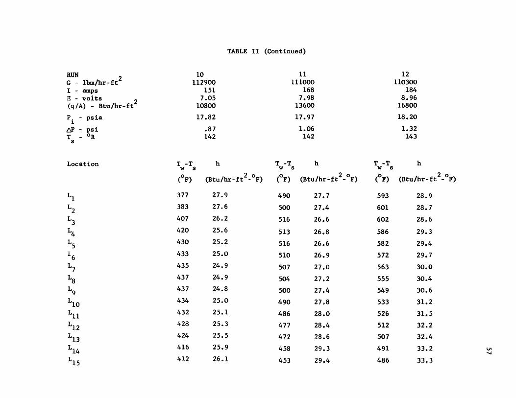
TABLE II (Continued)

RUNG - lbm/hr-ft2

I - ampsE - volts 2(q/A) - Btu/hr-ft 2

P. - psia

,& - psi

T - ORS

h

(Btu/hr-ft 2-o F)

27.9,

27.6

26.2

25.6

25.2

25.0

24.9

24.9

24.8

25.0

25.1

25.3

25.5

25.9

26.1

T -Tw s

( F)

490

500

516

513

516

510

507

504

500

490

486

477

472

458

453

h

(Btu/hr-ft -o F)

27.7

27.4

26.6

26.8

26.6

26.9

27.0

27.2

27.4

27.8

28.0

28.4

28.6

29.3

29.4

T -Tw 5

( F)

593

601

602

586

582

572

563

555

549

533

526

512

507

491

486

h

(Btu/hr-ft -o F)

28.9

28.7

28.6

29.3

29.4

29.7

30.0

30.4

30.6

31.2

31.5

32.2

32.4

33.2

33.3

10112900

1517.05

10800

17.82

.87142

11111000

1687.98

13600

17.97

1.06142

Location

12110300

1848.96

16800

18.20

1.32143

T -Tw (

( F)

L

L2L 3

L4L 516

L 7

L8L 9

L 10

Lii

L12L 13L 1

L 15

377

383

407

420

430

433

435

437

437

434

432

428

424

416

412

TABLE II (Continued)

RUNG - lbm/hr-ft2

I - ampsE - volts(q/A) - Btu/hr-ft 2

Pi - psia

AP - psiT - OR

s

h

(Btu/hr-ft -o F)

26.6

27.0

27.8

28.7

28.7

29.2

29.6

30.0

30.2

31.0

31.2

31.8

32.0

33.0

33.2

T -Tw s

(0F)

515

494

498

494

495

491

489

486

479

469

461

452

442

426

418

h

(Btu/hr-ft -o F)

33.8

35.0

34.8

35.2

35.0

35.2

35.4

35.5

36.0

36.5

36.9

37.4

38.0

39.2

39.7

T -Tw s

(0F)

590

556

554

544

544

537

533

527

519

502

491

477

468

450

442

h

(Btu/hr-ft -o F)

38.1

39.8

40.0

40.5

40.4

40.8

41.0

41.3

41.8

42.7

43.4

44.4

45.0

46.5

47.0

13110700

1849.0

16900

18.52

1.26143

14155200

1969.02

17100

18.87

1.57

143

15155200

2139.95

21600

19.26

2.16144

Location

L 1

L 2

L 3

L4

L 5

L 6

L 7

L 8

L 9

L 10

L 12

L 13

Li 1

L 15

T -Tw s(0F)

668

655

631

605

597

583

573

564

556

539

530

516

510

493

489

TABLE II (Continued)

RUN 2G - lbm/hr-ft2

I - ampsE - volts(q/A) - Btu/hr-ft 2

P. - psia

AP - gsiT -R

s

h

(Btu/hr-ft 2o F)

38.3

40.4

41.1

42.3

42.3

43.1

43.5

44.2

44.7

46.1

47.0

48.4

49.0

50.5

53.8

T -Tw s

( F)

394

411

414

421

427

429

428

429

424

422

416

414

404

393

387

h

(Btu/hr-ft -o F)

36.7

35.6

35.5

35.0

34.6

34.6

34.7

34.5

34.9

35.0

35.3

35.4

36.2

37.0

37.4

T -Tw s

( F)

444

530

460

458

468

470

472

472

466

458

450

440

429

412

403

h

(Btu/hr-ft 2-o F)

54.7

47.9

53.4

53.4

52.5

52.5

52.1

52.0

52.6

53.5

54.1

55.0

56.2

58.0

59.0

16154000

226.511.0

25400

19.65

2.34144

17157200

180.58.03

14700

18.67

1.35143

Location

18204000

229.510.4524400

20.42

2.53145

T -T( s

( 0F)

L2L 3

L4L 5

L 6

L 7

L8L 9L10L11

L 13L 1

L 1

710

658

638

615

612

598

588

577

565

542

528

510

500

480

475

TABLE II (Continued)

RUNG - lbm/hr-ftI - ampsE - volts 2(q/A) - Btu/hr-ft 2

P - psia

AP - gsiT -R

s

h

(Btu/hr-ft -o F)

54.0

48.6

53.5

54.0

53.0

52.9

52.7

52.5

53.3

54.5

55.1

56.2

57.4

59.5

60.5

T -Tw s

(0F)

344

425

392

385

395

404

407

412

410

410

406

403

393

380

375

h

(Btu/hr-ft -o F)

57.5

49.0

51.9

52.9

51.8

50.8

50.5

49.9

50.3

50.0

50.5

50.8

51.9

53.4

53.9

T -Tw s

(0F)

344

411

367

369

378

383

386

389

386

387

382

382

371

361

356

h

(Btu/hr-ft -o F)

48.0

41.7

44.8

45.5

44.4

44.0

43.8

43.6

43.9

43.6

44.1

44.1

45.3

46.3

46.7

19204000

24111.1

26300

20.73

2.86145

20205000

2159.3

20400

19.95

2.14

144

Location

21207000

1958.45

16800

19.63

1.86144

T -Tw (

(0F)

L

L 2

L 3

L4

L5

L6

L7

L8

L 9

L 10

L 12

L 13

L 15

486

565

494

491

502

503

504

503

495

482

474

461

450

430

422

TABLE II (Continued)

RUNG - lbm/hr-ft2

I - ampsE - volts(q/A) - Btu/hr-ft2

P - psia

AP - gsiT -R

s

h

(Btu/hr-ft 2o F)

46.5

40.9

41.0

42.0

41.0

40.2

40.0

39.5

39.8

39.4

39.4

39.4

40.3

40.9

41.0

T -Tw s

(0F)

231

252

272

264

267

279

282

291

289

300

293

304

295

295

293

h

(Btu/hr-ft -o F)

45.1

41.9

39.1

40.2

40.0

38.4

38.2

37.0

37.3

36.0

36.9

35.6

36.6

36.6

36.9

T -Tw s

( F)

187

191

208

214

211

223

226

236

234

249

243

259

248

251

251

h

(Btu/hr-ft -o F)

42.0

41.8

38.6

37.6

38.1

36.2

36.0

34.6

35.0

33.0

33.9

35.9

33.3

32.9

33.0

22211000

1787.55

13700

19.34

1.55144

23215000

1606.55

10700

19.03

1.34143

Location

24216000

142.55.628130

18.78

1.16143

T -Tw (

( 0F)

286

335

334

324

332

340

343

348

346

349

349

349

341

335

4332

L 10

Ly 1

L 12L 13Li 1L5

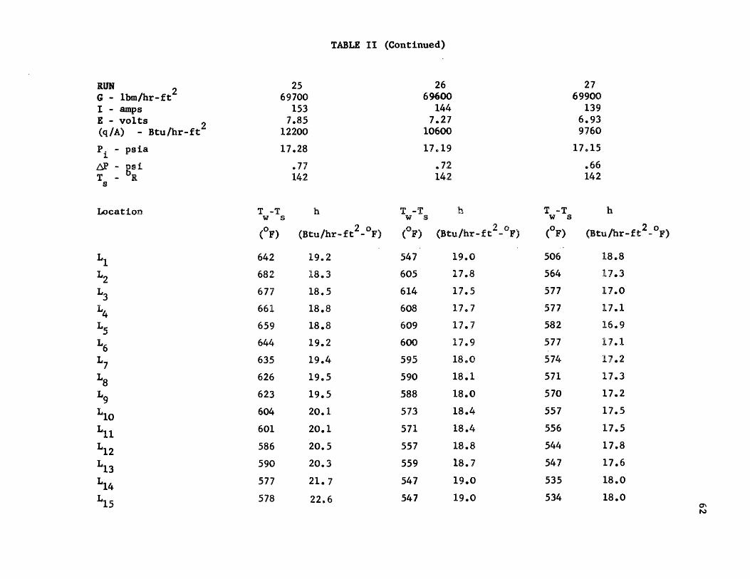
TABLE II (Continued)

RUNG - lbm/hr-ft2

I - ampsE - volts(q/A) - Btu/hr-ft 2

Pi - psia

AP - gsiT -R

s

h

(Btu/hr-ft 2-o F)

19.2

18.3

18.5

18.8

18.8

19.2

19.4

19.5

19.5

20.1

20.1

20.5

20.3

21. 7

22.6

T -Tw S

( 0 F)

547

605

614

608

609

600

595

590

588

573

571

557

559

547

547

h2

(Btu/hr-ft -o F)

19.0

17.8

17.5

17.7

17.7

17.9

18.0

18.1

18.0

18.4

18.4

18.8

18.7

19.0

19.0

T -Tw S

( F)

506

564

577

577

582

577

574

571

570

557

556

544

547

535

534

h

(Btu/hr-ft 2-o F)

18.8

17.3

17.0

17.1

16.9

17.1

17.2

17.3

17.2

17.5

17.5

17.8

17.6

18.0

18.0

2569700

1537.85

12200

17.28

.77142

2669600

1447.27

10600

17.19

.72142

Location

2769900

1396.939760

17.15

.66

142

T -Tw s

( 0F)

L3

L 2

L3

L4

L5

L6L 7

L8

L 9

L 10

L 1

L 12

L 13L 1

L 15

642

682

677

661

659

644

635

626

623

604

601

586

590

577

578

TABLE II (Continued)

RUNG - lbm/hr-ft2

I - ampsE - volts(q/A) - Btu/hr-ft 2

P - psia

AP - gsiT- R

s

b

(Btu/hr-ft 2o F)

18.6

17.3

16.7

16.6

16.3

16.3

16.3

16.3

16.2

16.4

16.4

16.7

16.6

16.9

16.9

T -Tw s

( F)

374

415

442

457

472

477

482

484

487

484

484

480

481474

474

h

(Btu/hr-ft -o F)

18.7

17.2

16.4

16.0

15.6

15.5

15.3

15.3

15.2

15.3

15.3

15.4

15.4

15.6

15.6

T -Tw s

( F)

320

353

381

400

418

428

435

441

447

447

449

448

449445

445

h

(Btu/hr-ft 2-o F)

18.8

17.3

16.4

15.7

15.1

14.9

14.6

14.5

14.3

14.3

14.3

14.3

14.3

14.4

14.4

2870000

1326.458600

17.04

.58142

2971000

1245.877320

17-04

.48142

3072000

1165.406320

16.98

.50141

Location

L 1

L 2

L4L5

L6

L 7

L8L 9

L 1

L 1

L 12

L 1

L14

L 15

T -Tw s

( F)

445

493

515

522

533

533

534

534

536

527

526

517

519509

508

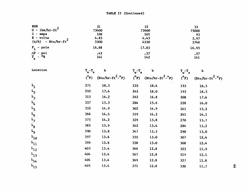
TABLE II (Continued)

RUN 2G - lbm/hr-ft2

I - ampsE - volts 2(q/A) - Btu/hr-ft 2

P - psia

AP - psiT - OR

5

h

(Btu/hr-ft 2-o F)

18.5

17.4

16.2

15.3

14.9

14.5

14.2

13.9

13.8

13.6

13.6

13.4

13.4

13.4

13.4

T -Tw 5

( F)

235

242

262

284

302

319

329

342

347

355

358

366

367

369

371

h

(Btu/hr-ft -o F)

18.4

18.0

16.8

15.6

14.9

14.2

13.8

13.4

13.3

13.0

13.0

12.8

12.8

12.8

12.8

T -Tw 5

( F)

193

193

208

228

241

261

270

284

290

307

308

323

319

327

330

h

(Btu/hr-ft -o F)

18.5

18.5

17.4

16.0

15.2

14.1

13.7

13.2

13.0

12.4

12.4

11.9

12.1

11.8

11.7

3173400

1084.855300

16.88

.43141

3273600

1014.454550

17.03

.37142

Location

3375000

933.973740

16.95

.37141

T -Tw (

0 F)

L 1

L 2

L 3

L4

L 5

L 6

L 7

L8

Lg 9

L 10

Li 1

L 12

L 13

Lg

L 15

271

292

315

337

352

366

375

385

390

397

399

403

404

404

405

TABLE II (Continued)

RUN 2 34 35 36G - lbm/hr-ft 119800 117700 114500I - amps 112 118 133E - volts 4.71 5.09 5.98(q/A) - Btu/hr-ft2 5340 6060 8060

P - psia 17.55 17.51 17.63

AP - psi .60 .60 .70T - OR 142 142 142

s

Location T -T h T -T h T -T hw S W S W s

( F) (Btu/hr-ft2 o F) ( F) (Btu/hr-ft 2-o F) ( F) (Btu/hr-ft -o F)

L 204 25.1 235 24.9 308 25.4

L2 212 24.3 237 24.8 314 25.0

L3 218 23.8 250 23.6 333 23.8

L4 233 22.4 267 22.3 349 22.9

L5 245 21.5 280 21.5 358 22.5

L6 260 20.4 294 20.6 365 22.2

L7 265 20.1 299 20.3 369 22.0

L8 275 19.5 308 19.8 374 21.7

L9 276 19.4 309 19.8 374 21.7

L10 287 18.7 319 19.3 377 21.6

L 285 18.9 317 19.4 375 21.7

L12 297 18.2 326 18.9 377 21.6

L13 291 18.6 321 19.2 374 21.7

L 294 18.4 322 19.2 370 21.9

L15 295 18.4 322 19.2 368 22.0

TABLE II (Continued)

RUNG - lbm/hr-ft2

I - ampsE - volts(q/A) - Btu/hr-ft 2

P - psia

AP - psiT - OR

S

h

(Btu/hr-ft -oF)

26.7

25.8

25.0

24.6

24.4

24.4

24.4

24.4

24.4

24.6

24.8

25.0

25.0

25.6

25.7

T -Tw s

( F)

555

551

547

536

534

525

520

516

512

498

493

481

478

464

459

h

(Btu/hr-ft - F)

25.2

25.3

25.5

26.0

26.1

26.4

26.5

26.6

26.7

27.4

27.6

28.1

28.1

28.9

29.1

T -Tw s

( F)

686

662

638

611

604

588

578

571

563

544

536

519

516

499

495

b

(Btu/hr-ft -o F)

25.8

26.5

27.2

28.1

28.2

28.8

29.2

29.4

29.7

30.5

30.7

31.5

31.5

32.5

32.6

37112700

1516.95

10600

17.72

.85142

38110100

1688.05

13700

17.92

1.01142

Location

39109600

1839.02

16800

18.13

1.28

143

T -Tw s

( 0F

L 1L 2

L 3

L4

L 5

L 6

L 7

L8

L 9

L 10

L 12

Li 1

L 15

391

407

424

433

439

439

439

439

437

434

430

426

422

412

408

TABLE II (Continued)

RUN 2G - lbm/hr-ft2

I - ampsE - volts 2(q/A) - Btu/hr-ft2

P - psia

AP - psi

Ts - OR

h

(Btu/hr-ft -o F)

27.2

28.5

29.6

30.6

31.0

31.8

32.1

32.6

32.8

34.0

34.4

35.3

36.5

39.6

41.8

T -Tw 8

( F)

705

638

620

602

600

587

578

570

558

536

523

506

496

476

472

h

(Btu/hr-ft2 F).

37.0

39.8

40.6

41.5

41.4

42.0

42.5

42.8

43.5

45.0

46.0

47.1

47.5

49.0

50.6

T -Tw s

( F)

576

540

536

529

531

524

520

515

507

493

483

471

461

444

436

b

(Btu/hr-ft -o F)

36.8

38.5

38.6

39.2

38.9

39.4

39.6

40.0

40.4

41.2

41.8

42.0

43.2

44.4

45.1

40110000

20010.0

20400

18.55

1.64

143

41153800

22210.8

24400

19.33

2.30

144

Location

42154800

2079.65

20400

18.95

1.94143

T -T( s

( F)

L 1

L 2

L3

L4

L5

L6L 7

L8

L 9L 10

L 12

L 13

L 15

816

763

721

683

672

648

635

621

612

586

576

557

556

540

540

TABLE II (Continued)

RUNG - lbm/hr-ft2

I - ampsE - volts(q/A) - Btu/hr-ft 2

P - psia

AP - gsiT -R

s

h

(Btu/hr-ft2 o F)

36.9

37.2

37.0

37.1

36.8

36.8

36.9

36.9

37.2

37.6

37.9

38.3

39.0

40.0

40.6

T -Tw s

( F)

351

389

377

388

396

400

401

404

403

402

397

396

388

379

375

h

(Btu/hr-ft -o F)

38.0

35.2

36.0

35.2

34.7

34.4

34.4

34.3

34.3

34.3

34.6

34.6

35.2

35.9

36.2

T -Tw s

( F)

241

281

281

291

304

316

321

327

327

335

331

337

331

329

327

h

(Btu/hr-ft -o F)

40.4

35.4

35.6

34.5

33.2

32.2

31.8

31.2

31.4

30.6

31.0

30.4

31.0

31.2

31.4 os

43156200

1918.65

16800

18.67

1.59

143

44158000

1747.75

13700

18.44

1.30

143

Location

45164200

1546.50

10150

18.11

1.06143

L I

L 2

L 3

L4

L 5

L6

L 7

L8

Lg 9

L 10

Li 1

L 12

L 13

Li 1

L 15

T -Tw s

( F)

458

453

456

458

462

461

460

459

454

447

441

435

426

412

405

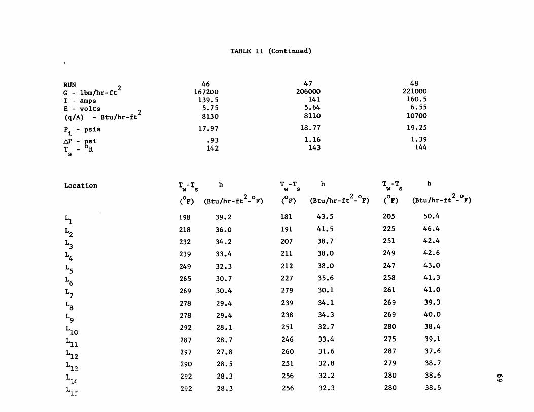
TABLE II (Continued)

RUNG - lbm/hr-ft2

I - ampsE - volts(q/A) - Btu/hr-ft 2

P - psia

A? - psiT - OR

s

46167200

139.55.758130

17.97

.93142

T -Tw (

( 0F)

198

218

232

239

249

265

269

278

278

292

287

297

290

292

292

h

(Btu/hr-ft -o F)

39.2

36.0

34.2

33.4

32.3

30.7

30.4

29.4

29.4

28.1

28.7

27.8

28.5

28.3

28.3

47206000

1415.648110

18.77

1.16143

T -Tw S

( F)

181

191

207

211

212

227

279

239

238

251

246

260

251

256

256

h

(Btu/hr-ft -o F)

43.5

41.5

38.7

38.0

38.0

35.6

30.1

34.1

34.3

32.7

33.4

31.6

32.8

32.2

32.3

T -Tw s

( F)

205

225

251

249

247

258

261

269

269

280

275

287

279

280

280

48221000

160.56.55

10700

19.25

1.39144

h

(Btu/hr-ft -o F)

50.4

46.4

42.4

42.6

43.0

41.3

41.0

39.3

40.0

38.4

39.1

37.6

38.7

38.6

38.6

Location

L 1

L 2

L 3

L4

L 5

L 6

L 7

L8L 9

L 10L 1

L 12

Ll3

L

TABLE II (Continued)

RUNG - ibm/hr-ftI - ampsE - volts(q/A) - Btu/hr-ft 2

P - psia

AP - psiT - OR

S

h

(Btu/hr-ft -o F)

53.0

46.8

42.6

45.1

44.6

43.7

43.2

42.4

42.6

41.7

42.2

41.5

42.3

42.8

43.0

T -Tw S

( F)

311

390

365

357

365

370

373

378

376

377

373

373

365

355

351

h

(Btu/hr-ft -o F)

52.4

44.0

46.4

46.9

46.1

45.6

45.3

44.9

45.1

44.9

45.3

45.2

46.1

47.3

47.6

T -Tw S

( F)

345

434

402

390

400

407

411

415

413

412

408

403

394

381

375

h

(Btu/hr-ft 2-o F)

57.4

48.0

50.7

52.1

51.0

50.4

50.0

49.5

49.9

49.9

50.3

50.8

51.8

53.3

53.9

49216000

179.57.55

13800

19.43

1.62

144

50211000

195.58.45

16800

19.67

1.88144

Location

51209000

2149.35

20400

20.06

2.22144

T -Tw S

( F)

L

L 2

L 3

4

L 5

L6

L 7

L8L 9

110Lio

L12

L 13

L 15

250

291

325

303

307

315

320

327

326

334

330

335

328

324

322

TABLE II (Continued)

RUNG - lbm/hr-ft2

I - ampsE - volts(q/A) - Btu/hr-ft

P. - psia

AP - psiT - OR

s

h

(Btu/hr-ft2 o F)

58.7

49.7

55.9

56.3

54.9

54.6

54.6

54.3

54.7

55.5

56.1

57.3

58.2

60.3

61.0

T -Tw s

( F)

502

597

513

509

519

519

519

517

509

493

484

469

459

438

430

h

(Btu/hr-ft 2-o F)

58.2

51.4

57.3

57.9

56.9

56.9

56.9

56.7

57.5

59.1

60.0

61.5

62.4

64.6

65.5

T -Tw s

( F)

770

785

762

731

724

701

687

672

667

645

640

624

630

621

624

h

(Btu/hr-ft 2-o F)

19.2

19.0

19.4

19.8

20.0

20.4

20.7

21.0

21.2

21.6

21.7

23.0

24.0

25.6

27.0

52206000

23310.6

25200

20.50

2.67143

53205000

24911.5

29200

20.95

3.10145

Location

5470000

1608.73

14200

17.91

.97142

T -Tw s

( 0F)

L 1

L 2

L 3L4

L 5

5

L 6

L 7

L 8

L 9

L 1

L 1

L 1L13

L14

15

423

527

452

449

461

464

465

468

463

455

448

438

428

410

402

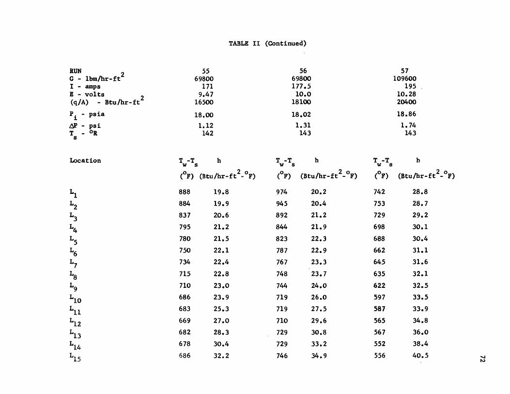
TABLE II (Continued)

RUN 2G - lbm/hr-ft2

I - ampsE - volts 2(q/A) - Btu/hr-ft 2

P - psia

AP - psi

T - ORs

h

(Btu/hr-ft -o F)

19.8

19.9

20.6

21.2

21.5

22.1

22.4

22.8

23.0

23.9

25.3

27.0

28.3

30.4

32.2

T -Tw s

( F)

974

945

892

844

823

787

767

748

744

719

719

710

729

729

746

h

(Btu/hr-ft -o F)

20.2

20.4

21.2

21.9

22.3

22.9

23.3

2307

24.0

26.0

27.5

29.6

30.8

33.2

34.9

T -Tw s

( F)

742

753

729

698

688

662

645

635

622,

597

587

565

567

552

556

h

(Btu/hr-ft -o F)

28.8

28.7

29.2

30.1

30.4

31.1

31.6

32.1

32.5

33.5

33.9

34.8

36.0

38.4

40.5

5569800

1719.47

16500

18.00

1.12142

5669800177.5

10.018100

18.02

1.31143

Location

57109600

19510.2820400

18.86

1.74143

T -Tw a

(0F)

L 1

L 2

L3

L4

L 5

L 6

L 7

L8LB

L, 1

L 12

L 13

L 15

888

884

837

795

780

750

734

715

710

686

683

669

682

678

686

TABLE II (Continued)

RUNG - lbm/hr-ft2

I - ampsE - volts 2(q/A) - Btu/hr-ft 2

P - psia

A? - psiT - OR

s

58110000

20510.9222800

19.40

2.18144

T -Tw S

( F)

828

812

774

737

724

695

676

662

647

620

610

587

594

582

593

h

(Btu/hr-ft -o F)

29.5

29.8

30.8

31.8

32.2

33.1

33.7

34.3

34.8

35.8

36.2

39.0

40.8

44.0

46.4

59110000

214.511.6225400

19.62

2.44

144

T -Tw S

( F)

912

866

821

780

765

730

707

691

676

648

640

620

634

629

650

60156800

190.59.17

17800

19.17

1.84143

b

(Btu/hr-ft -o F)

30.4

31.4

32.4

33.6

34.0

35.0

35.6

36.2

36.8

38.2

40.3

44.2

45.9

49.5

51.8

T -Tw S

( F)

513

508

513

509

508

501

498

496

487

475

466

455

446

430

423

h

(Btu/hr-ft -o F)

35.3

35.4

35.3

35.4

35.4

35.8

36.0

36.0

36.5

37.3

37.8

38.4

39.0

40.2

40.7

Location

L 1

L 2

L 3

L4

L 5

L 6

L 7

L8

L 9

L 10

L 12

Li 1

Li 1

TABLE II (Continued)

RUN 61 62G - ibm/hr-ft2 154900 154500

I - amps 221.5 225E - volts 11.22 11.54

(q/A) - Btu/hr-ft2 25300 26500

P. - psia 20.09 20.17

AP - gsi 2.69 2.80T - R 144 144

S

Location T -T h T -T s

(0F) (Btu/hr-ft 2-o F) ( F) (Btu/hr-ft -o F)

L 674 39.4 702 39.8

L2 662 39.8 687 40.3

L3 650 40.3 672 40.9

L 634 41.0 654 41.8

L5 632 41.1 650 47.9

L6 613 42.0 630 42.9

L7 601 42.5 617 43.4

L8 592 42.9 606 43.9

L 576 43.7 590 44.7

L10 550 45.3 562 46.3

L 536 46.0 546 47.2

L12 513 47.5 523 48.8

L13 507 48.0 520 49.0

L 488 49.4 501 52.0

L15 487 52.1 502 54.7

j

I p

[A

Fig. 1 Photograph of the Nitrogen Film Boiling Test Apparatus

Steam Supply

Ammeter Voltmeter

11OV

I Valve

Steam

Pressure Seal '

Nitrogen Supply

FIGURE 2

System Pressure_,, -Control Valve

Nitrogen

Test Section Discharge

Thermocouples(quantitative testsection only)

Lucite Tube

Pressure Tap

Flow Control Valve

Flash Cooler

Radiation Shield

Bleed Control Valve

Vacuum Chamber

Insulated NitroqenSupply Tube Connection

Regulated HeliumPressure Source

SCHEMATIC DIAGRAM OF THE NITROGEN FILM BOILING TESTAPPARATUS.

Thermometer

:- Apparatus Support Frame

White Backgroundand Reflector

Black Light Shield

M icrof lash

VisualTestSection

UnipodSliding

withClamp

Camera

a) Layout with White Background.

Black Background

"-White Ref lector-

>Black Light ShieldM icrof lash

b) Arrangement of Block Background

Figure 3 Schematic Plan View of the Photographic Layout.

111'

a) Vapor Quality Range:0% to 6%

b) Vapor Quality Range5% to 11%

Fig. 4 Film Boiling Inside a Vertical Tube

a) Vapor Quality Range:34% to 41%

b) Vapor Quality Range:43% to 50%

Fig. 5 Film Boiling Inside a Vertical Tube

Vapor Quality Range: 34% to 41%

Fig. 6 Film Boiling Inside a Vertical Tube

BT Uhr-ftf G u 70,000 Ibm/hr-ft2

200r .o 7

0 10 20 30 40 50 60 70 80 90 100 110 120 130 140 150L/D

FIGURE 7 WALL SUPERHEAT VARIATION ALONG THE TUBE

1000

950

900

850

750

L 600

550

900

u-0

850-

800-

750-

700-

650-

600-

550-

500

450

400

350

300

250

200

150

100

O 10 20 30 40 50 60 70 80 90 0010 120 130 140 150L/D

FIGURE 8 WALL SUPERHEAT VARIATION ALONG THE TUBE

RUN Q BTUNO. A ~hr-ft2

2G~ 160,000 Ibm/hr-ft

I I I I I I I I I I I I I I

0 0 02 40 60 80L/D

SUPERHEAT VARIATION

750

00 25300

25400

700-

650 6

600-

550-

500-

450-

400

350-

300-

250-

200-

150-

100-

U-0

Cl)H-

H-

14701( ii)17 oil

137004 4

..................

50100 120 140

ALONG THE TUBEFIGURE 9 WALL

10 20 30 40 50 60 70 80 90 100 110L/ D

120 130 140 150

SUPERHEAT VARIATION

750

700

650

600

550

500

450

400

350

300

250

200

150

100

50

ALONG THE TUBEFIGURE 10 WALL

i IRUN NO.55

I I I LG-Ibm /hr-ftI I I I I I I I I

O- -

A- - =6980017000 BTU/ hr-ft 2

8000 BTU/hr-ft 2

900-

850-

800-

750-

700-

650 -

600-

550-

500-

450-

400-

109600

70000

28

5OA, 211000

50|

200

167200

0- .-----. o .-

- 4o4,-* 2 16000o-f I I I

. .... 0-

-

... ..- -- ~

10 20 30 40 50 60 70 80 90 100 120 130 140 150 160L/D

FIGURE II EFFECT OF FLOW RATE ON WALL SUPERHEATVARIATION ALONG THE TUBE

39

350

300 - 36 _o_._o--...--o--o--0..... 0 _- -- l"""

n | I I I I I I

NN

.~-.-- -. ___ - - - ®- .- ~.---------- - - -~m.--m--=---._- - - -~

- -~

I I I I I I I I I I I -I -10 20 30 40 50 60 70 80 90

L /D

100 110 120 130 140

FIGURE 12 TYPICAL NUSSELT NUMBER VARIATION ALONG THE

TUBE.

180 -

170-

160-

150-

140-

130-

120-

101-

70 H

60

50 F

40

30-

20 -

10 -

150

"100 -

90 -

80 -

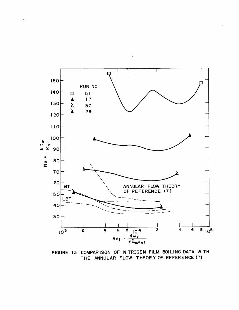
I I IEl

RUN NO.5117

3729

ANNULAR FLOW THEORYOF REFERENCE (7)

LBT - .

77

I I I II I I I I I I I

4 6 84 6 8 104

Ref =TDwp vf

FIGURE 13 COMPARISON OF NITROGEN FILM BOILING DATA WITHTHE ANNULAR FLOW- THEORY OF REFERENCE (7)

150-

140 ~

130-

120-

110-

z

100-

90-

80-

70-

60 -BT

50

40

30-

10 3 105I I I I I I I

1100 -

1050-

1000-

950-

900-

850-

800-

750-

700-

650-

600-

550-

500-

450-

400-

350-

300-

250-

200-

150-

100-

50-

0-0

FIGURE 14 EFFECT OF PROPERTY EVALUATION ON THE

DITTUS - BOELTER EQUATION

40 80 120 160 200 240 280

L/D

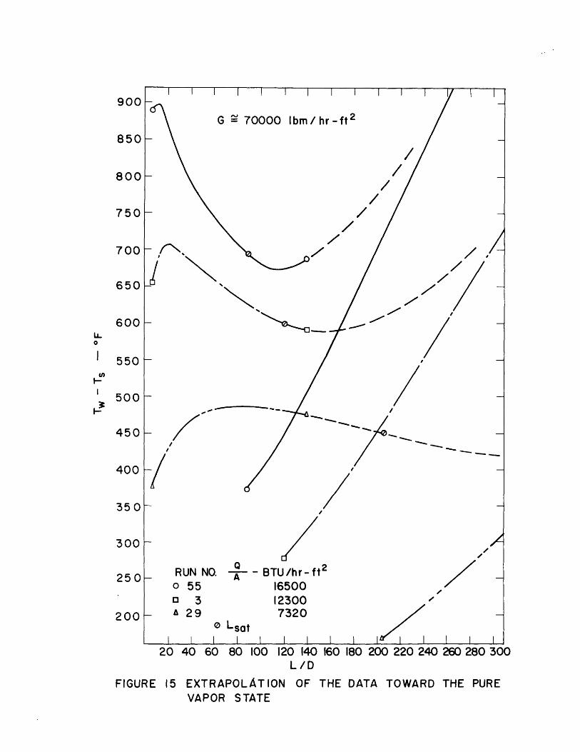
20 40 60 80 100 120 140 160 180 200 220 240 260 280 300L/D

FIGURE 15 EXTRAPOLATION OF THE DATA TOWARD THE PUREVAPOR STATE

900

850

800

750

700

650

600

550

500

450

400

350

300

250

200

LiL0

U)

I-x

300 -

y 250 -

200-

RUN NO. BTU /hr - f t2150 *Ao 53 29200

100o- 51 20400o Lsot

50-

0 I I I I I I I

20 40 60 80 100 120 140 160 180 200 220 240 260 280 300L/D

FIGURE 16 EXTRAPOLATION OF THE DATA TOWARD THE PUREVAPOR STATE

450

400- 0 3o 29v 70 53

350- 4 22A 47

300-

250-

200- 0--~~

150-

0 10 20 30 40 50L -INCHES

FIGURE 17 CALCULATED

a

10-

VAPOR TEMPERATURE

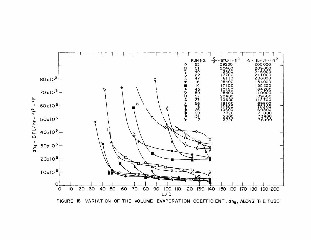
80xI0 3 - 47 8110 206000* 16 25400 154000

* 14 17100 15520070 A 45 10150 164200

0xlO 59 25400 110000

40xlO3_0 1060

0 37 10600 1 127000X 56 18100 6980060xO3- * 3 12300 70200

.9 26 10600 69800S29 7320 71000

5\\\ 31 5300 73400

5~- 0x103 - No 70 60

o 0 _

:D 3I 3

mm2013 A

20x 103

0 10 20 30 40 50 60 70 80 90 100 110 120 130 140 150 160 170 180 190 200L/D

COEFFIClENT, ahe, ALONG THE TUBEFIGURE 18 VARIATI0N OF THE VOLUME EVAPORATION

HEATED LENGTH - L/Dw

DROPLET ACCELERATION ANALYSIS

200

180

160

140

120

100

80

60

40

20

0140

FIGURE 19

1000 I I I I I I I I I I

0

00

100 L

C,,M

RUN NO.o 310 3* 22i 510 53

| | | | | | |

0-BTU/hr-f t2

530012300137002040029200

G-Ibm/hr-ft 2

7340070200

211000209000204000

I I I >14±.10

I-X

FIGURE 20 CALCULATED MEAN EFFECTIVE DROP SIZE

101.1I

I I | I | | | |

I I I I I I I I

1000

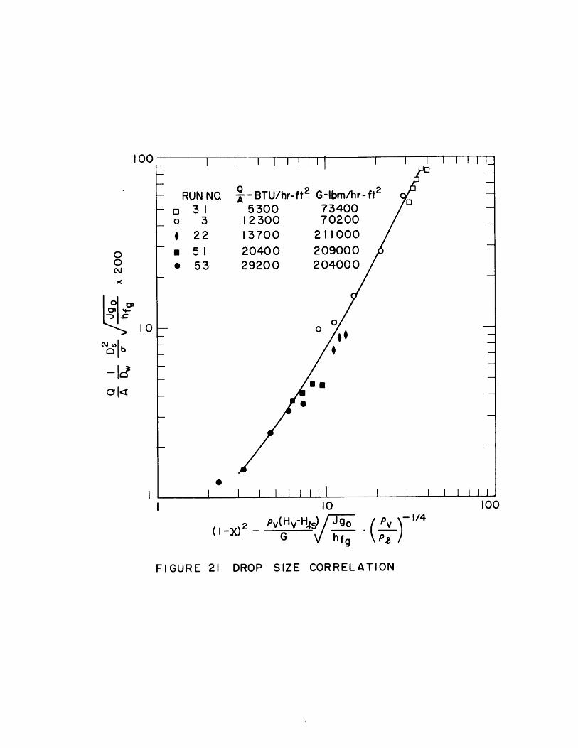
100 - I I 1111111 I I I I

RUN NO 2- BTU/hr-ft 2 G-3 1 5300 7

3 12300 722 13700 2151 20400 2053 29200 20

0

| | | | |

10

(I-X)2 _ Pv(Hy-H Jg(I-X - G hf g

Ibm/hr-ftp2

34000200100090004000

I - I I I I I I I

( V )-1/

DROP SIZE CORRELATION

-coS0

0

10ib

100

FIGURE 21

I I I I I I I I

100 I i 1 i i 1 1 1 -

-/

0.9

0.8-

0.7/

0.6-

0.5

0.4-

0.3-

0.2--MINIMUM QUALITY FOR DISPERSED FLOW THEORYUPPER LIMIT OF EXPERIMENTAL DATA

0.1 0 G 210000 Ibm/hr -ft 2' G 160000 Ibm/ hr -ft 2

0 G 1 15000 Ibm/hr -ft 2

4 G'~ 70000 Ibm /hr-ft 2

0 5000 10000 15000 20000 25000 30000

--- BTU/hr-ft 2

FIGURE 22 REGION OF VALIDITY OF THE DISPERSEDFLOW THEORY

1.0-

0.9-b

0.8-

0.78- b Xbx0.7 - . o x

0.6- 0 o 4 o

0.5- 0 b x Q0 RUN NO. -BTU/hr-ft 2 G- Ibm/hr-ft 2

0 - 0 53 29200 2050000 51 20400 209000v 49 13800 216000

22 13700 21 1000

0.3 - e 16 25400 154000a 14 171OO 155200A 45 10150 164200

0.2 b 59 25400 110000t2 57 20400 109600A 37 10600 112700x 56 18100 69800

0.1 3 123007000. -* 26 000 698004 0 320 734060

0 0.2 0.4 0.6 0.8 1.0 1.2 1.4 1.6 1.8L/ Lsat

OF THE FILM BOILING PROCESS FROM AN EQUILIBRIUM CONDITIONFIGURE 23 DISPLACEMENT

I I 1 I

//

/

20

15

0f-

5[-

OH-

-5

I I I I I I I400 500

Tw -Ts -*F600 700 800 900

FIGURE 24 THERMAL LOSSES FROM THE OUTER SURFACE OF THE TEST SECTION

100 200 300

o UPPER LIMIT FROM3. BOILING TEST DATA r

3.0 ss

2.5 2.5 - 00--- LOWER LIMIT FROMH- BOILING TEST DATA

- 2.0

C,)

1.5

-300 -200 -100 0 100 200 300 400 500 600 700TEMPERATURE -F

RESISTIVITY OF THE 304 STAINLESS STEEL TEST SECTIONFIGURE 25 ELECTRICAL