Systemic risk at high frequency: price cojumps and Hawkesfactor models

Fabrizio Lillo

Scuola Normale Superiore di Pisa, University of Palermo (Italy) and Santa Fe Institute (USA)

FisMat2013 - Milan, September 9, 2013

1 / 31

In collaboration with

This project has been developed in QuantLab:

G. BormettiL.M. Calcagnile

F. CorsiS. Marmi

M. TreccaniQUANT

QuantLab is a joint Research Lab between SNS & List Spa.See www.quantlab.it

2 / 31

Motivations

Financial markets are intrinsically unstable and display large pricefluctuations

Often these fluctuations occur on very short time scales, and sometimesrevert quickly.

It is commonly believed that in recent year there has been an increasingfrequency of these events

Neither idiosyncratic news nor market wide news can explain the frequencyand amplitude of price jumps (Joulin et al. 2008)

Nanex research suggested a sharp increase of price jump frequency andrelated it to market regulation

“when rebalancing their positions, High Frequency Traders may competefor liquidity and amplify price volatility” (Kirilenko et al. 2010)

Flash crash was not only about E-Mini S&P 500 futures (where everythingstarted), but propagated in a very short time to ETFs, stocks, options, etc

3 / 31

Price jumps

Price jumps are discontinuities in the price process.

Mathematically it is typically described by a compound Poisson noise term inthe price equation

Xt =

∫ t

0

µsds +

∫ t

0

σsdWs +

Nt∑l=1

Jt

4 / 31

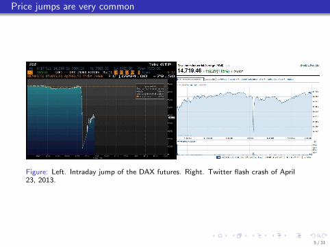
Price jumps are very common

Figure: Left. Intraday jump of the DAX futures. Right. Twitter flash crash of April23, 2013.

5 / 31

May 6, 2010 Flash Crash

On May 6, 2010 markets dropped 1% per minute, reaching a low of morethan 10%During the flash crash 8 stocks in the S&P500 were traded at 1 cent (e.g.Accenture). Others (e.g. Apple and Hewlett-Packard) were traded at100,000$There is growing concern about the possible role of High Frequency Traderas responsible of large price jumps“when rebalancing their positions, High Frequency Traders may competefor liquidity and amplify price volatility” (Kirilenko et al. 2010)

6 / 31

Stock price jumps and systemic risk

Flash crash was not only about E-Mini S&P 500 futures (where everythingstarted)

Because of arbitration, when the e-Mini changes price with high volume,Many ETFs are repriced (quotes updated, trades executed).The component stocks of ETFs are also repriced, along with many indexes.All the option chains for the ETFs, their components and indexes are alsorepriced.

Trades being executed at irrational prices as low as one penny or as highas $ 100,000

Flash crash: a 20 millesecond cascade (Nanex)

HFTs as means of contagion (Gerig 2012)

Motivation for our study: how frequent are systemic events? How can wemodel them?

7 / 31

Questions

Dynamics of jumps: (Bormetti et al., Modelling systemic price cojumpswith Hawkes factor models, arXiv:1301.6141)

Is there a dynamics of jumps? Does a jump change the probability ofanother jump in the near future? Time clustering of jumps?Is there a contagion between jumps in different assets? Cross-assetexcitation of jumps?How frequent are systemic co-jumps?

Have market become more unstable in recent years?Have markets become more ”jumpy” in recent years?Is the contagion of jumps across assets faster today? Are market moreexposed to systemic events?

8 / 31

Data description

Data Sample

Tick by Tick Data of FTSE 40 Italy, traded at Milan stock exchange

20 high liquidity stocks

88 Days of Executions (March-June 2012)

One minute time scale for log returns

Jump detection methods are obviously very sensitive to outliers, dataanomalies, etc.

Outlier removal: Brownlees - Gallo (2006) algorithm

Merging / Splitting and Volatility auctions are automatically subtracted

Removal of intraday volatility pattern

We need a statistically robust identification method for jumps

9 / 31

Jumps identification

Most of the jump identification methods are essentially estimating thelocal volatility and then testing that the ratio between absolute return andvolatility is above a given threshold

This approach implicitly requires the definition of a time scale used tocompute returns (in our case, one minute)

We defineJump:

|r |σ> θ (we choose θ = 4 as in Bouchaud et al., 2008)

The volatility estimation is the most critical step and differentiatesmethods

We used the realized bipower variation (Barndorff-Nielsen and Shephard(2003, 2004)

σ̂2bv,t = µ−2

1 |ri ||ri+1| = µ−21 α

∑i>0

(1− α)i−1|rt−i ||rt−i−1|,

with µ1 =√

2π' 0.797885 and α = 0.032 (gives 50% of weight to the

closest 22 observations).

10 / 31

Number of detected jumps

ISIN jumps jumps up jumps down single jumps cojumps

IT0000062072 103 48 (47%) 55 (53%) 53 (51%) 50 (49%)IT0000062957 63 29 (46%) 34 (54%) 38 (60%) 25 (40%)IT0000064482 121 60 (50%) 61 (50%) 97 (80%) 24 (20%)IT0000068525 93 46 (49%) 47 (51%) 56 (60%) 37 (40%)IT0000072618 127 67 (53%) 60 (47%) 55 (43%) 72 (57%)IT0001063210 59 28 (47%) 31 (53%) 44 (75%) 15 (25%)IT0001334587 178 73 (41%) 105 (59%) 150 (84%) 28 (16%)IT0001976403 123 61 (50%) 62 (50%) 76 (62%) 47 (38%)IT0003128367 188 81 (43%) 107 (57%) 107 (57%) 81 (43%)IT0003132476 155 66 (43%) 89 (57%) 95 (61%) 60 (39%)IT0003487029 70 28 (40%) 42 (60%) 41 (59%) 29 (41%)IT0003497168 129 74 (57%) 55 (43%) 79 (61%) 50 (39%)IT0003856405 95 50 (53%) 45 (47%) 74 (78%) 21 (22%)IT0004176001 74 41 (55%) 33 (45%) 46 (62%) 28 (38%)IT0004231566 103 50 (49%) 53 (51%) 72 (70%) 31 (30%)IT0004623051 115 47 (41%) 68 (59%) 85 (74%) 30 (26%)IT0004644743 100 51 (51%) 49 (49%) 65 (65%) 35 (35%)IT0004781412 118 49 (42%) 69 (58%) 57 (48%) 61 (52%)LU0156801721 59 27 (46%) 32 (54%) 32 (54%) 27 (46%)NL0000226223 86 39 (45%) 47 (55%) 51 (59%) 35 (41%)

total 2159 1015 1144

average 108.0 50.8 (47%) 57.2 (53%)

11 / 31

Multiple cojumps in the Italian stock market

Time series of the number of stocks n co-jumping simultaneously

9 10 11 12 13 14 15 16 17

Hour

Mar

Apr

May

Jun

Jul

Day

n = 12 ≤ n ≤ 3

4 ≤ n ≤ 8

9 ≤ n ≤ 20

A large number of cojumps involving a sizable number of assets!

12 / 31

Comparing with independent Poisson processes

9 10 11 12 13 14 15 16 17

Hour

Mar

Apr

May

Jun

JulDay

0 10 20

Number of cojumping stocks

0

1

2

3

log10(counts)

Left. Simulated independent multivariate Poisson process with intensities as inreal data. Right. Histogram of the number of stocks jumping simultaneously inone minute. Real data (filled circles) vs. independent Poisson model (emptycircles).

There is a large number of jumps per stock: ≈ 1.2 jumps per stock per day

At the daily scale, the number of jumps is Poisson distributed

There is a large number of “simultaneous” jumps of groups of stocks, notexplained by Poisson

Can we identify evidence of time clustering of jumps on the same or ondifferent assets?

13 / 31

A multi-scale statistical test based on multiple jumps and cross jumpsdetection

A multiple jump (MJ) of a stock is the event of at least two jumps of thestock’s price occurring inside a time window.A cross-jump (CJ) between two stocks is the event of at least one jump in theseries of each stocks occurring inside a given time window.

si the number of jumps in window i of length w

estimator for multiple jump probability in a window of length w over asampling period of length N

p̂MJw =

∑b Nw ci=1 1si≥2⌊

Nw

⌋ ,

estimator for cross-jump probability of stock l and k in a window of lengthw between stock l and k

p̂CJw =

∑b Nw ci=1 1s li≥11ski ≥1⌊

Nw

⌋ .

For each window length w we estimate empirically these quantities and wecompare with 99% and 95% confidence bands of the tested null model

We correct for multiple hypothesis testing using Bonferroni correction

14 / 31

Testing multiple jumps for individual stocks under the Poisson null

0 50 100

w (minute)

0

0.02

0.04

0.06

p̂M

Jw

EmpiricalPoisson meanPoisson 99% c.l.

Poisson 95% c.l.

Figure: MJ probability test under Poisson null for the Italian asset Assicurazioni Generali.

In our data sample the null is rejected for 18 stocks out of 20.⇒ Strong evidence of time clustering of jumps and violation of the univariatePoisson model.

15 / 31

Dynamic Intensity Models: Hawkes Processes

Hawkes Processes (Hawkes, 1971)A univariate point process Nt is called a Hawkes process if it is a linearself-exciting process, defined by the intensity

I (t) = λ(t) +

∫ t

−∞ν(t − u)dN(u) ,

where λ is a deterministic function called the base intensity and ν is a positivedecreasing weight function.The most common parametrization of ν is given by ν(t) =

∑Pj=1 αje

−βj t , fort > 0, where αj ≥ 0 are scale parameters, βj > 0 controls the strength ofdecay, and P ∈ N is the order of the process.For single exponential kernel and λ(t) constant, the expected number of jumpsin a time interval of length T is

E[∫ t0+T

t0

dNt

]=

λ

1− α/βT .

16 / 31

Hawkes processes

0 5 10 15 20

0.0

0.5

1.0

1.5

2.0

2.5

3.0

Time

IntensityEvents

Time0 0 011 1 1 1 1 1 12 2 2 22 22 2 23 3 3 34

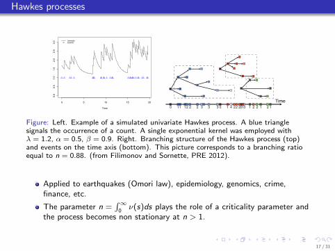
Figure: Left. Example of a simulated univariate Hawkes process. A blue trianglesignals the occurrence of a count. A single exponential kernel was employed withλ = 1.2, α = 0.5, β = 0.9. Right. Branching structure of the Hawkes process (top)and events on the time axis (bottom). This picture corresponds to a branching ratioequal to n = 0.88. (from Filimonov and Sornette, PRE 2012).

Applied to earthquakes (Omori law), epidemiology, genomics, crime,finance, etc.

The parameter n =∫∞

0ν(s)ds plays the role of a criticality parameter and

the process becomes non stationary at n > 1.

17 / 31

Testing multiple jumps for individual stocks under Null Hawkes

0 10 20 30

w (minute)

0

0.005

0.01

0.015

p̂M

Jw

EmpiricalMonte Carlo meanMonte Carlo 99% c.l.

Monte Carlo 95% c.l.

0 250 500

w (minute)

0

0.25

0.5

Figure: MJ probability test under Hawkes null for the assets Assicurazioni Generali (left)and Intesa Sanpaolo (right).

⇒ Univariate Hawkes processes are able to capture the dynamics and timeclustering of jumps of real data

18 / 31

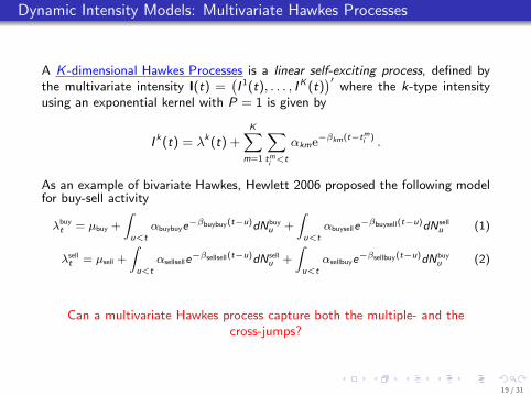
Dynamic Intensity Models: Multivariate Hawkes Processes

A K -dimensional Hawkes Processes is a linear self-exciting process, defined bythe multivariate intensity I(t) =

(I 1(t), . . . , IK (t)

)′where the k-type intensity

using an exponential kernel with P = 1 is given by

I k(t) = λk(t) +K∑

m=1

∑tmi <t

αkme−βkm(t−tmi ) .

As an example of bivariate Hawkes, Hewlett 2006 proposed the following modelfor buy-sell activity

λbuyt = µbuy +

∫u<t

αbuybuye−βbuybuy(t−u)dNbuy

u +

∫u<t

αbuyselle−βbuysell(t−u)dN sell

u (1)

λsellt = µsell +

∫u<t

αsellselle−βsellsell(t−u)dN sell

u +

∫u<t

αsellbuye−βsellbuy(t−u)dNbuy

u (2)

Can a multivariate Hawkes process capture both the multiple- and thecross-jumps?

19 / 31

Failure of the bivariate Hawkes models

0 10 20 30

w (minute)

0

0.005

0.01

0.015

p̂CJ

w

EmpiricalMonte Carlo meanMonte Carlo 99% c.l.

Monte Carlo 95% c.l.

Figure: CJ probability test under independent Hawkes null for the pair of Italian assetsGenerali - Intesa Sanpaolo.

Multivariate Hawkes processes fail to describe both the single stock andthe cross stock time clustering of jumps observed in real data

When calibrated on real data, Hawkes processes strongly underestimatethe “simultaneous” jumps of stocks.

20 / 31

1 Factor Model with 2 Stocks

Main idea: A single factor model of jumps of a set of stocks

There is one (unobserved) market factor point process describing thejumps

When the factor jumps, stock k jumps with probability pk

A stock can jump also because of an idiosyncratic point process

In equations,I k(t) = v k(t)λF (t) + λk(t) (3)

where v k(t) ∼ B(1, pk) and λF (t) and λk(t) are the intensities of the factorpoint process and of the idiosyncratic process, respectively.

Note that the number of parameters to estimate goes down from O(N2) toO(N).

21 / 31

A toy example: 2 Stocks without idiosyncratic terms

Without idiosyncratic terms the only variable to specify is the point processdescribing the factor

Poisson factor: λF (t) = λPoisson

Hawkes factor: λF (t) = λHawkes(t)

p1p2λFT = n12

p1λFT = n1 =⇒ P1,P2, λF

p2λFT = n2

where n1 and n2 are the realized number of jumps of the stock 1 and 2, whilen12 represents the realized number of cojumps between 1 and 2 within the oneminute sampling interval.

Easy to implement with 2 stocks

No unique way to extend to multi stocks

22 / 31

One Factor Poisson model (without idiosyncratic terms)

● ● ● ● ● ● ● ● ● ● ● ● ● ● ● ●●

●●

●●

●

●

0 5 10 15 20 25 30

0.00

00.

002

0.00

40.

006

0.00

8

Self−cojumping probability of IT0000062072

Windows length

Coj

umps

freq

uenc

y

● ● ● ● ● ● ● ● ● ● ● ● ● ● ● ● ● ● ● ● ● ● ●● ● ● ●● ● ● ●

●

● ● ● ●

●●

●

●

●

●

●

●

●

●

● ● ● ● ● ● ● ● ● ● ● ● ● ● ● ● ● ● ● ● ● ● ●● ● ● ● ● ●● ● ● ●

● ● ● ● ● ●

●●

●

●●

●

●

● ● ●●

●●

●

●●

●

●●

●

●

● ●

●

●

●

●

● ●

●

oooo

observedMC meanMC 99% c. l.MC 95% c. l.

●●

●●

●●

●●

●●

●●

●●

●●

●

●

●

●

●

●

●

0 5 10 15 20 25 30

0.00

00.

005

0.01

00.

015

0.02

00.

025

0.03

0

Cross−cojumping probability of IT0000062072 and IT0000072618

Windows length

Coj

umps

freq

uenc

y

● ● ● ● ● ●● ●

● ●● ●

● ● ●●

● ●

●●

●● ●

●●

●●

●

●●

●●

●●

●

●●

●

●

●

●

●

●

●

●

●

●● ● ● ● ●

● ●●

●●

●● ●

●●

●●

●

●●

●●

●●

●●

●●

●●

●●

●●

●●

●●

●

●

●

●

●

●

●

●●

●●

●●

●●

● ● ● ●

● ● ●●

●

● ●

●

●

● ●

oooo

observedMC meanMC 99% c. l.MC 95% c. l.

Figure: Multiple (left) and cross (right) jump probability test against a null modelspecifically designed for two stocks: single stock jumps are generated by the thinningof a systemic factor driven by a Poisson process. The number of Monte Carlo paths is103.

⇒ The factor term explains the cross-cojumps, but the Poissonianity of thefactor leads to underestimation of self-cojumps (as expected).

23 / 31

1 Factor Model + Idiosyncratic with 20 stocks

Consider the whole set of 20 Stocks and define

{tsi } for i = 1, . . . , ns , set of event times for the s-th stock

{tFj } for j = 1, . . . , nF , set of event times when the realized number ofcross-cojumps rejects the null hypothesis of cross independence

{tsi′} = {tsi } \ {tFj } ⊆ {tsi } for i ′ = 1, . . . , ns′ , subset of event times for thes-th stock compatible with the null of cross-independence

We introduce a kind of recursive Expectation-Maximization algorithm toestimate

The parameters describing the point processes of the factor and of theidiosyncratic terms

The systemic (factor) jumps and the idiosyncratic jumps

The main technical problem is to distinguish when a multiple jumps is due to ajump of the (unobservable) factor and when it is due to multiple idiosyncraticjumps.

24 / 31

Test multiple and cross jumps under a null with One Factor Hawkes +Idiosyncratic Hawkes

0 10 20 30

0

0.005

0.01

p̂M

Jw

EmpiricalMonte Carlo meanMonte Carlo 99% c.l.

Monte Carlo 95% c.l.

0 10 20 30

0

0.005

0.01

p̂CJ

w

0 10 20 30

w (minute)

0

0.005

0.01

0 10 20 30

w (minute)

0

0.01

0.02

p̂CJ

w

Figure: From the top left clockwise: MJ probability test under N factor model null forthe asset Generali; CJ probability test for the pairs Generali-Mediobanca,Generali-Banca Popolare Milano, and Generali-Intesa Sanpaolo.

25 / 31

Are financial markets becoming more and more unstable?

There is a growing concern that financial markets have become moreunstable, i.e. the number of price jumps have increased in recent years

HFTs have been blamed to be responsible for the increased instability

Our contribution: an historical investigation of the evolution of marketinstabilities at high frequency

Data: The set of the 120 most liquid assets of the Russell 3000 index inthe period 1999-2012

Need for a careful definition of price jumps

0.5

1.0

1.5

2.0

1−m

inut

e vo

latil

ity

Jan−

00

Jan−

01

Jan−

02

Jan−

03

Jan−

04

Jan−

05

Jan−

06

Jan−

07

Jan−

08

Jan−

09

Jan−

10

Jan−

11

Figure: Left. Number of shocks according to a Credit Suisse report. Right. Volatilityof our Russell 3000 data.

26 / 31

Systemic cojumps

020

000

4000

060

000

8000

0

jumps

2000

2001

2002

2003

2004

2005

2006

2007

2008

2009

2010

2011

010

020

030

040

050

060

0

10−asset cojumps

2000

2001

2002

2003

2004

2005

2006

2007

2008

2009

2010

2011

020

4060

8010

0

30−asset cojumps

2000

2001

2002

2003

2004

2005

2006

2007

2008

2009

2010

2011

010

2030

60−asset cojumps

2000

2001

2002

2003

2004

2005

2006

2007

2008

2009

2010

2011

Figure: Evolution of single asset jumps (top left), 10-asset cojumps (top right),30-asset cojumps (top right), and 60-asset cojumps (top right)

Total number of jumps and the number of single asset jumps have actuallydeclined in recent yearsThe number of multiple asset co-jumps have increased significantlyThis effect is stronger for systemic cojumps, i.e. cojumps involving a largenumber of assets

27 / 31

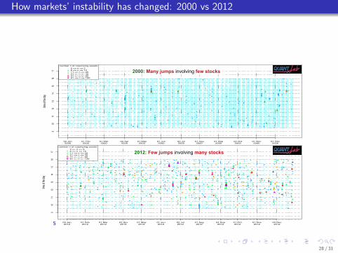
How markets’ instability has changed: 2000 vs 2012

5

2000: Many jumps involving few stocks

2012: Few jumps involving many stocks

28 / 31

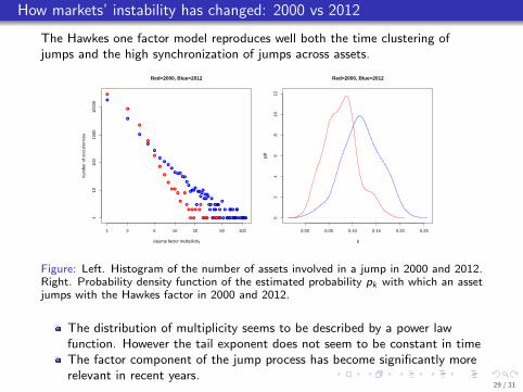
How markets’ instability has changed: 2000 vs 2012

The Hawkes one factor model reproduces well both the time clustering ofjumps and the high synchronization of jumps across assets.

●

●

●

●

●

●

●●

●

● ● ●

●●

●

●

●●●●

●

●●

●

●●

●

●

●

●●

●

●

●

●

●●

●

●

●

●

●●●

●

●

●

●

●

●

●●●●

●●

●

●

●●●●●

●●

● ●●●●●●●●

1 2 5 10 20 50 100

110

100

1000

1000

0

Red=2000, Blue=2012

cojump factor multiplicity

num

ber

of o

ccur

renc

es

●

●

●

●

●

●

●

●

● ●

●

●

●

●

●

●

●

●

● ●

●

●●●● ●● ●●

0.00 0.05 0.10 0.15 0.20 0.25

02

46

810

12

Red=2000, Blue=2012

p

pdf

Figure: Left. Histogram of the number of assets involved in a jump in 2000 and 2012.Right. Probability density function of the estimated probability pk with which an assetjumps with the Hawkes factor in 2000 and 2012.

The distribution of multiplicity seems to be described by a power lawfunction. However the tail exponent does not seem to be constant in timeThe factor component of the jump process has become significantly morerelevant in recent years.

29 / 31

Systemic cojumps and news arrival

Systemic cojumps: Exogenously triggered or endogenously generated?In order to test for the exogenous hypothesis, we consider the news feedmam.econoday.com focusing on macro announcementsWe compute the fraction of systemic cojumps of N assets which arepreceeded by a news in the previous 1-5 minutes

●●●●●●●●●●●●●●●●●●●●●●●●●●●●●●●●●●●●●●●●●●●●

●●●●●●●●●●●●●●●●●●●

●●●●●●●●●●●●●●●●

●●●

●

●●●●●●●●●●●●●●●●●●●●●●●●●●●●●

0 20 40 60 80 100

0.0

0.2

0.4

0.6

0.8

1.0

cojump factor multiplicity

Pro

babi

lity

of a

new

s tr

igge

r

●●●●●●●●●●●●●●●●●●●●●●●●●●●●●●●●●●●●●●●●●●●●

●●●●●●●●●●●

●●●●●●●●

●●●●

●●●●●●●

●●●●●

●●●

●

●

●●●●●●●●●●●●●●

●●

●

●●

●●

●●

●●●●●

●●●●●●●●●●●●●●●●●●●●●●●●●●●●●●

●●●●●

●●●●

●●●●●●●

●●●●●●●●●●●●●●

●●●

●●●●

●●●●●

●●●●

●●●

●●●●

●

●●●●●●●●

●●●●●●

●●

●

●●

●●

●●

●●●●●

●●●●●●●●

●●●●●●●●●●●●●●●●●●●●●●

●●●●

●●●●●

●●●●●

●●●●●●●●●●●

●●●●●●●●

●●●●

●●●●●

●●●●

●

●●

●●●●

●

●●●●●●●●

●●●●●●

●●

●

●●

●●

●●

●●●●●

●●●●●

●●●●●●●●●●●●●●●●●

●●●●●

●●●●

●●●

●●●●●●

●●●●

●●●●●●●●●●●

●●●●●●●●

●●●●

●●●●●

●●●●

●

●●

●●●●

●

●●●●●●●●

●●●●●●

●●

●

●●

●●

●●

●●●●●

Figure: Fraction of systemic cojumps which are preceeded by a macro news in theprevious 1 (black), 2 (cyan), 3 (blue), 4 (green), or 5 (red) minutes as a function ofthe number of jumping assets.

Only approximately 30− 40% of the large systemic cojumps can be associatedwith macro news (for example FOMC announcements)Are the other systemic cojumps endogenously generated?

30 / 31

Conclusions

A large number of jumps are present in financial markets

On individual stocks, jumps are clearly not described by a Poisson process,but display time clustering well described by Hawkes processes

We identify a very large number of simultaneous and systemic co-jumps,i.e. sizable sets of stocks “simultaneously” jumping

We propose a Hawkes one factor point process model which is able todescribe

1 The time clustering of jumps on individual stocks2 The time lagged cross excitation between different stocks3 The large number of “simultaneous” systemic jumps

Individually, stocks have become less ”jumpy” in recent years

However the frequency of systemic jumps has considerably increased

Systemic cojumps are only marginally related to news

31 / 31