Fabrizio Colonna, Stefania Marcassa To cite this version

HAL Id: hal-00869315https://hal.archives-ouvertes.fr/hal-00869315

Preprint submitted on 2 Oct 2013

HAL is a multi-disciplinary open accessarchive for the deposit and dissemination of sci-entific research documents, whether they are pub-lished or not. The documents may come fromteaching and research institutions in France orabroad, or from public or private research centers.

L’archive ouverte pluridisciplinaire HAL, estdestinée au dépôt et à la diffusion de documentsscientifiques de niveau recherche, publiés ou non,émanant des établissements d’enseignement et derecherche français ou étrangers, des laboratoirespublics ou privés.

Taxation and Labor Force Participation: The Case ofItaly

Fabrizio Colonna, Stefania Marcassa

To cite this version:Fabrizio Colonna, Stefania Marcassa. Taxation and Labor Force Participation: The Case of Italy.2013. �hal-00869315�

https://hal.archives-ouvertes.fr/hal-00869315

https://hal.archives-ouvertes.fr

Taxation and Labor Force Participation:The Case of Italy

Fabrizio Colonna∗

Stefania Marcassa†

January 24, 2013

Abstract

Italy has the lowest labor force participation of women among European countries. Moreover,

the participation rate of married women is positively correlated to their husbands’ income. We show

that a high tax schedule together with tax credits and transfers raise the burden of two-earner house-

holds, generating disincentives to work. We estimate a structural labor supply model for women,

and use the estimated parameters to simulate the effects of alternative revenue-neutral tax systems.

We find that joint taxation implies a drop in the participation rate. Conversely, working tax credit

and gender-based taxation boost it, with the effects of the former concentrated on low educated

women.

Keywords: female labor force participation, Italian tax system, second earner tax rate, joint taxa-

tion, gender-based taxation, working tax credit

JEL Classification: J21, J22, H31

∗Banca d’Italia, Economic Structure and Labor Market Division, Department for Structural Economic Analysis,via Nazionale 91, 00184 Roma, IT. Email: [email protected]†Corresponding author. Universite de Cergy-Pontoise THEMA (UMR CNRS 8184), 33 boulevard du Port, 95011

Cergy-Pontoise cedex, FR. Email: [email protected]. A previous version of paper has been presented atthe conference “Women and the Italian Economy” organized by the Bank of Italy, held in Rome on March 7th, 2012.The views expressed therein are those of the authors and do not necessarily reflect those of the Bank of Italy.

1

1 Introduction

The labor force participation of Italian women is the lowest among most European countries. More-

over, while the labor force participation of married women is usually negatively correlated to their

husbands’ incomes, in Italy the correlation is positive. In this paper, we argue that the taxation

system partly explains the coexistence of these two features.

Our interest in this topic is motivated by the anemic growth rate of the Italian economy over

the last decade. A low labor force participation is an immediate explanation for a stagnant GDP,

especially when combined with a declining population. But there is also a public policy issue: if

whatever makes Italy’s participation rate low involves a distortion rather than a choice, then there is

room for improvement in both income and welfare. These considerations are in line with Europe2020,

the European Union Commission’s growth strategy that targets five objectives on employment,

innovation, education, social inclusion and climate/energy by 2020.1 In particular, Italy has set

the target for the employment rate to 67-69 percent, implying an increase of about 6 percentage

points. Moreover, Italy has committed to a decrease of about 2.2 million of people at-risk-of-poverty,

meaning a reduction of 18 percent of the population in this critical situation.2

In order to reach these objectives, it is crucial to identify reforms that promote labor force

participation in the short-term, mainly for those groups of population that are not well represented

in the labor market. Our work goes in the direction of suggesting alternative taxation systems that

would boost women’s participation by about 3 percentage points, and decrease the percentage of

women who are below the poverty line by up to 2 percentage points.

The Italian taxation system is based on an individual tax unit. It is characterized by a high

tax schedule, a set of tax credits for children and for the spouse who is not employed, as well as

cash transfers for dependent children. The combination of these elements raises the tax burden,

especially on two-earner households, generating disincentives to participate in the labor force for

1A detailed description can be found here: http://ec.europa.eu/europe2020/index_en.htm.2In 2008, the population at-risk-of-poverty in Italy was 19 percent of the total, that is about 12 million of people.

See http://epp.eurostat.ec.europa.eu/cache/ITY_OFFPUB/KS-SF-10-009/EN/KS-SF-10-009-EN.PDF.

2

http://ec.europa.eu/europe2020/index_en.htm

http://epp.eurostat.ec.europa.eu/cache/ITY_OFFPUB/KS-SF-10-009/EN/KS-SF-10-009-EN.PDF

married women, typically the second earner of the family. Such disincentives are stronger when the

first earner’s income is low. More specifically, tax credits and universal cash transfers are decreasing

functions of the household income. This means that their incidence on the second earner tax rate

decreases in total income, providing incentives to participate that are higher for richer households.3

The second earner tax rate is also increasing in the number of children, and reaches a maximum at

husbands’ yearly earnings of about 8, 000 euros for childless couples, and 19, 000 euros for couples

with children. Furthermore, the difference between the second earner tax rate of married and

unmarried women is large at low incomes, and becomes negligible at higher earnings, discouraging

part-time and low skill jobs.4

We use micro data from the EU-SILC (2007-2008) to estimate a structural model of labor supply

that includes, as main ingredient, the characteristics of the Italian tax system.5 We model the labor

supply decision of women as sequential. First, they decide whether to search for an occupation, and

upon receiving a job offer, they accept it or not. Men’s labor supply and incomes are given. All of

the labor decisions depend on the net yearly income, hence on the characteristics of the taxation

system. The model is able to generate the low level of the participation rate, as well as the positive

correlation between women’s participation rate and husbands’ income. It also matches the part-time

and full-time employment rates.

Then, we use the estimated parameters to measure the behavioral effects of alternative (revenue

neutral) tax systems: joint family taxation (in line with the French system), a system inspired by the

(British and American) working tax credit, a gender-based taxation (as proposed by Alesina et al.

[2011]), and a mixture of the Italian and the joint taxation system. We assume that the simulated

3The second earner tax is the amount of tax paid on an additional unit of income when the second earner worksrelatively to the case in which she is unemployed or out of the labor force.

4While the increase in more favorable conditions of part-time jobs may create incentives for (married) mothersto participate in the labor market, Manning and Petrongolo [2008] provide evidence of part-time jobs as potentialsources of occupational segregation.

5In general, the choice of participating in the labor market depends upon several variables. It reflects the valueassigned to domestic activities as housework and child care (Olovsson [2009]), and the amount of wealth owned.Moreover, social norms play an important role in the decision of women to work, especially in Italy. The World ValueSurvey reports that 80 percent of the Italian population, of both genders, thinks that a child younger than 3 yearsold suffers if the mother works. Even thought we recognize the importance of these variables in determining the laborsupply decision, we do not include them in our analysis.

3

tax systems are characterized by the same taxation rates, but differ in the set of tax credits and

transfers.

We show that the joint tax system implies a substantial drop in female labor participation of

married women. In particular, the decrease in the participation rate is increasing in the husband’s

income. On the contrary, the working tax credit and the gender-based system boost the participation

rate of all women. The effects of the former concentrates on unskilled and low educated women (and

hence, low skill and part-time jobs). In the latter, the reduced tax burden generates a positive shift

of the participation rate. But, the tax credits for dependent spouse and children leave unchanged

the negative incentives for low income households. The mixture system allows to choose the taxation

system that implies the lowest tax. The effects on the labor force participation and employment are

intermediary between those produced by the two systems separately. The Italian system is chosen

for low levels of income, as it gives right to receive tax credits and transfers for children. For higher

incomes, households prefer the joint taxation system, as they benefit from the quotient familial.6

Finally, we compare the effects on welfare of these systems by computing several poverty measures

for the women in the sample. We show that the gender-based system increases the well-being of

unmarried women, reducing the transfer needed to reach the poverty line. On the contrary, married

women are better off in the mixture system.

Our paper is placed in the context of three main strands of literature. First, it relates to

recent works which argue that the taxation system may create a set of incentives to labor force

participation, and that it may play an important role in explaining cross-country differences in labor

supply behavior. Some examples are Prescott [2004], Davis and Henrekson [2004], Rogerson [2006],

and Olovsson [2009].

Second, our work belongs to the rich stream of the empirical labor supply analysis, both for the

U.S. and Europe. A fundamental role in addressing the relevance of taxation has been played by

6The quotient familial has been adopted in France since 1945. It aims to make the amount of the income taxproportional to households’ ability to pay. It consists of a coefficient by which the total household revenue has to bedivided. It is a function of the number of household components, and each member has a different weight dependingon being adult or child. See Saint-Jaques [2009] for a detailed description of the French system.

4

Burtless and Hausman [1978], Hausman [1980], and Hausman [1985]. Our paper uses a framework

similar to Colombino and Del Boca [1990]. We enrich their results by showing that the model is able

to reproduce the positive correlation between wife’s labor force participation rate and husband’s

income. Moreover, in the statistical procedure for the wage prediction, we correct for selection

bias using a non-linear method which accounts for the probability that an individual with given

characteristics opts for a certain labor supply choice.

Third, several studies examine the effect of tax reforms on labor force participation. Up to twenty

years ago, the theoretical literature on taxation converged to an optimal scenario characterized by a

basic income transfer and an almost flat income tax. More recently, the literature focused on in-work

benefits (Colombino et al. [2000], Saez [2002], Immervoll et al. [2007], Mooij [2008], and Blundell

et al. [2011]). Several studies have evaluated the expected labor supply effects from introducing in-

work tax credits in the U.S. and U.K. The most recent and relevant studies are for the U.K. Blundell

et al. [2000] and Blundell and Hoynes [2003], and for the U.S. Meyer and Rosenbaum [2001] and

Fang and Keane [2004]. The results from these studies suggest that there are strong incentive effects

from tax credits. The broadening of the tax credit seems to have contributed to the increase in

labor force participation and to reduce welfare participation. Our results are also consistent with

the findings of Eissa and Liebman [1996], Cavalli and Fiorio [2006], and Bar and Leukhina [2009].

This paper is organized as follows. In Section 2, we provide a description of the Italian labor

market and taxation system. In Section 3, we specify the empirical strategy, we describe the data,

and present the results. In Section 4, we measure the behavioral effects of alternative tax systems.

Section 5 concludes.

5

2 Labor Market and Taxation System in Italy

2.1 Empirical Evidence

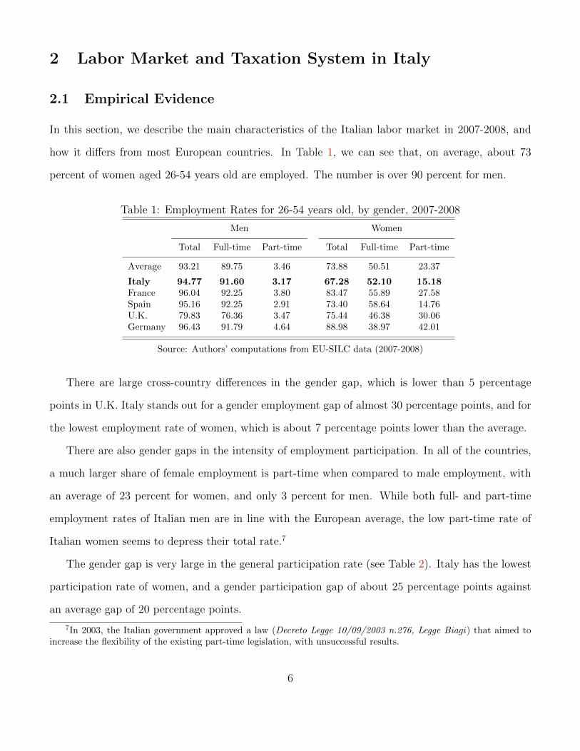
In this section, we describe the main characteristics of the Italian labor market in 2007-2008, and

how it differs from most European countries. In Table 1, we can see that, on average, about 73

percent of women aged 26-54 years old are employed. The number is over 90 percent for men.

Table 1: Employment Rates for 26-54 years old, by gender, 2007-2008

Men Women

Total Full-time Part-time Total Full-time Part-time

Average 93.21 89.75 3.46 73.88 50.51 23.37

Italy 94.77 91.60 3.17 67.28 52.10 15.18France 96.04 92.25 3.80 83.47 55.89 27.58Spain 95.16 92.25 2.91 73.40 58.64 14.76U.K. 79.83 76.36 3.47 75.44 46.38 30.06Germany 96.43 91.79 4.64 88.98 38.97 42.01

Source: Authors’ computations from EU-SILC data (2007-2008)

There are large cross-country differences in the gender gap, which is lower than 5 percentage

points in U.K. Italy stands out for a gender employment gap of almost 30 percentage points, and for

the lowest employment rate of women, which is about 7 percentage points lower than the average.

There are also gender gaps in the intensity of employment participation. In all of the countries,

a much larger share of female employment is part-time when compared to male employment, with

an average of 23 percent for women, and only 3 percent for men. While both full- and part-time

employment rates of Italian men are in line with the European average, the low part-time rate of

Italian women seems to depress their total rate.7

The gender gap is very large in the general participation rate (see Table 2). Italy has the lowest

participation rate of women, and a gender participation gap of about 25 percentage points against

an average gap of 20 percentage points.

7In 2003, the Italian government approved a law (Decreto Legge 10/09/2003 n.276, Legge Biagi) that aimed toincrease the flexibility of the existing part-time legislation, with unsuccessful results.

6

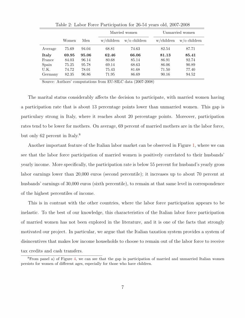
Table 2: Labor Force Participation for 26-54 years old, 2007-2008

Married women Unmarried women

Women Men w/children w/o children w/children w/o children

Average 75.69 94.04 68.81 74.63 82.54 87.71

Italy 69.95 95.06 62.46 66.06 81.13 85.41France 84.03 96.14 80.68 85.14 86.91 92.74Spain 75.25 95.78 69.14 68.63 86.06 90.89U.K. 74.72 78.01 75.43 81.68 71.50 77.40Germany 82.35 96.86 71.95 86.69 90.16 94.52


The marital status considerably affects the decision to participate, with married women having

a participation rate that is about 13 percentage points lower than unmarried women. This gap is

particulary strong in Italy, where it reaches about 20 percentage points. Moreover, participation

rates tend to be lower for mothers. On average, 69 percent of married mothers are in the labor force,

but only 62 percent in Italy.8

Another important feature of the Italian labor market can be observed in Figure 1, where we can

see that the labor force participation of married women is positively correlated to their husbands’

yearly income. More specifically, the participation rate is below 55 percent for husband’s yearly gross

labor earnings lower than 20,000 euros (second percentile); it increases up to about 70 percent at

husbands’ earnings of 30,000 euros (sixth percentile), to remain at that same level in correspondence

of the highest percentiles of income.

This is in contrast with the other countries, where the labor force participation appears to be

inelastic. To the best of our knowledge, this characteristics of the Italian labor force participation

of married women has not been explored in the literature, and it is one of the facts that strongly

motivated our project. In particular, we argue that the Italian taxation system provides a system of

disincentives that makes low income households to choose to remain out of the labor force to receive

tax credits and cash transfers.

8From panel a) of Figure 4, we can see that the gap in participation of married and unmarried Italian womenpersists for women of different ages, especially for those who have children.

7

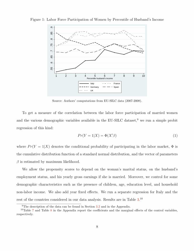
Figure 1: Labor Force Participation of Women by Percentile of Husband’s Income

.55

.6.6

5.7

.75

.8.8

5.9

1 2 3 4 5 6 7 8 9 10Percentile husband’s income

Italy France

Germany Spain

UK

Source: Authors’ computations from EU-SILC data (2007-2008).

To get a measure of the correlation between the labor force participation of married women

and the various demographic variables available in the EU-SILC dataset,9 we run a simple probit

regression of this kind:

Pr(Y = 1|X) = Φ(X ′β) (1)

where Pr(Y = 1|X) denotes the conditional probability of participating in the labor market, Φ is

the cumulative distribution function of a standard normal distribution, and the vector of parameters

β is estimated by maximum likelihood.

We allow the propensity scores to depend on the woman’s marital status, on the husband’s

employment status, and his yearly gross earnings if she is married. Moreover, we control for some

demographic characteristics such as the presence of children, age, education level, and household

non-labor income. We also add year fixed effects. We run a separate regression for Italy and the

rest of the countries considered in our data analysis. Results are in Table 3.10

9The description of the data can be found in Section 3.2 and in the Appendix.10Table 7 and Table 8 in the Appendix report the coefficients and the marginal effects of the control variables,

respectively.

8

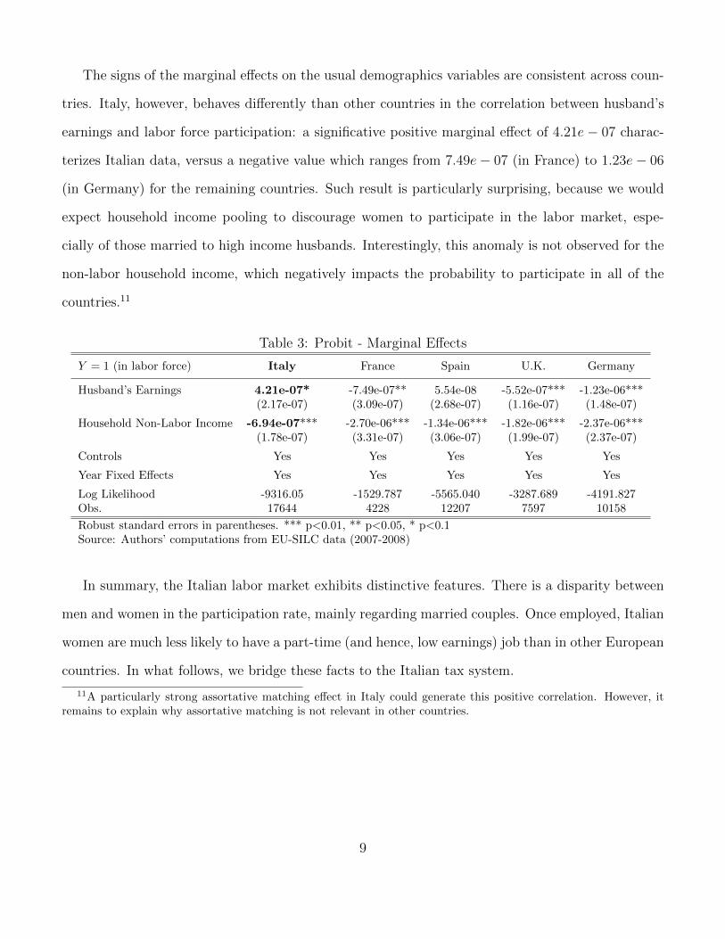
The signs of the marginal effects on the usual demographics variables are consistent across coun-

tries. Italy, however, behaves differently than other countries in the correlation between husband’s

earnings and labor force participation: a significative positive marginal effect of 4.21e − 07 charac-

terizes Italian data, versus a negative value which ranges from 7.49e− 07 (in France) to 1.23e− 06

(in Germany) for the remaining countries. Such result is particularly surprising, because we would

expect household income pooling to discourage women to participate in the labor market, espe-

cially of those married to high income husbands. Interestingly, this anomaly is not observed for the

non-labor household income, which negatively impacts the probability to participate in all of the

countries.11

Table 3: Probit - Marginal Effects

Y = 1 (in labor force) Italy France Spain U.K. Germany

Husband’s Earnings 4.21e-07* -7.49e-07** 5.54e-08 -5.52e-07*** -1.23e-06***(2.17e-07) (3.09e-07) (2.68e-07) (1.16e-07) (1.48e-07)

Household Non-Labor Income -6.94e-07*** -2.70e-06*** -1.34e-06*** -1.82e-06*** -2.37e-06***(1.78e-07) (3.31e-07) (3.06e-07) (1.99e-07) (2.37e-07)

Controls Yes Yes Yes Yes Yes

Year Fixed Effects Yes Yes Yes Yes Yes

Log Likelihood -9316.05 -1529.787 -5565.040 -3287.689 -4191.827Obs. 17644 4228 12207 7597 10158

Robust standard errors in parentheses. *** p<0.01, ** p<0.05, * p<0.1Source: Authors’ computations from EU-SILC data (2007-2008)

In summary, the Italian labor market exhibits distinctive features. There is a disparity between

men and women in the participation rate, mainly regarding married couples. Once employed, Italian

women are much less likely to have a part-time (and hence, low earnings) job than in other European

countries. In what follows, we bridge these facts to the Italian tax system.

11A particularly strong assortative matching effect in Italy could generate this positive correlation. However, itremains to explain why assortative matching is not relevant in other countries.

9

2.2 The Italian Tax System

In this section, we describe the main characteristics of the Italian taxation system. More technical

details can be found in the Appendix.

We define the second earner of a household as the worker with the highest elasticity of labor

supply to income. Generally, in a married couple, the husband is considered to be the first earner,

who participates in the labor market with certainty. The wife is the second earner. Her decision to

participate depends on several economic and non economic variables. In particular, it depends on

the fraction of her expected gross income that will be disposable, net of total taxes. To understand

the impact of taxes on the decision to work, we make use of the concept of second earner tax rate.

Let us define the second earner tax rate (SET) as follows:

SET ≡ ∆T

yf=Tax(ym, yf )− Tax(ym, 0)

yf

where Tax(ym, yf ) and Tax(ym, 0) are the total income taxes paid by the household if the wife

works and if she does not work, respectively. yf is her gross income when she works, and ym is the

husband’s gross income. We assume that her income is equal to zero when she does not work (i.e.

she is either out of the labor force or unemployed).

Now, depending on the unit of the fiscal system (individual or family), the second earner tax

rate and the average tax rate of a married woman may be significantly different than those of an

unmarried woman.12

In Italy, however, we should not observe a marital status dependence of the amount of tax paid,

because the tax system is based on the individual and not on the household. Nevertheless, tax

credits for family dependents and universal cash transfers for children are decreasing functions of

the household income and indirectly affect the fiscal burden related to the labor force participation

status of the wife. Hence, the SET can be expressed as the sum of the tax rate of wife and a

distortion which depends on tax credits (TaxCred) and universal cash transfers (UnivCash), in the

12The average tax rate is the ratio between the total household taxes and the gross household income.

10

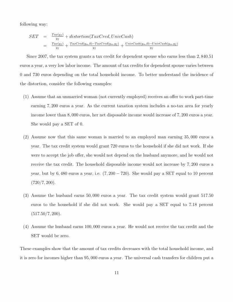
following way:

SET =Tax(yf )

yf+ distortion(TaxCred, UnivCash)

=Tax(yf )

yf+

TaxCred(ym,0)−TaxCred(ym,yf )

yf+

UnivCash(ym,0)−UnivCash(ym,yf )

yf

Since 2007, the tax system grants a tax credit for dependent spouse who earns less than 2, 840.51

euros a year, a very low labor income. The amount of tax credits for dependent spouse varies between

0 and 730 euros depending on the total household income. To better understand the incidence of

the distortion, consider the following examples:

(1) Assume that an unmarried woman (not currently employed) receives an offer to work part-time

earning 7, 200 euros a year. As the current taxation system includes a no-tax area for yearly

income lower than 8, 000 euros, her net disposable income would increase of 7, 200 euros a year.

She would pay a SET of 0.

(2) Assume now that this same woman is married to an employed man earning 35, 000 euros a

year. The tax credit system would grant 720 euros to the household if she did not work. If she

were to accept the job offer, she would not depend on the husband anymore, and he would not

receive the tax credit. The household disposable income would not increase by 7, 200 euros a

year, but by 6, 480 euros a year, i.e. (7, 200− 720). She would pay a SET equal to 10 percent

(720/7, 200).

(3) Assume the husband earns 50, 000 euros a year. The tax credit system would grant 517.50

euros to the household if she did not work. She would pay a SET equal to 7.18 percent

(517.50/7, 200).

(4) Assume the husband earns 100, 000 euros a year. He would not receive the tax credit and the

SET would be zero.

These examples show that the amount of tax credits decreases with the total household income, and

it is zero for incomes higher than 95, 000 euros a year. The universal cash transfers for children put a

11

similar mechanism at work in married households. On the contrary, they have the positive effect of

reducing the fiscal burden of unmarried mothers, and create positive incentives to their participation

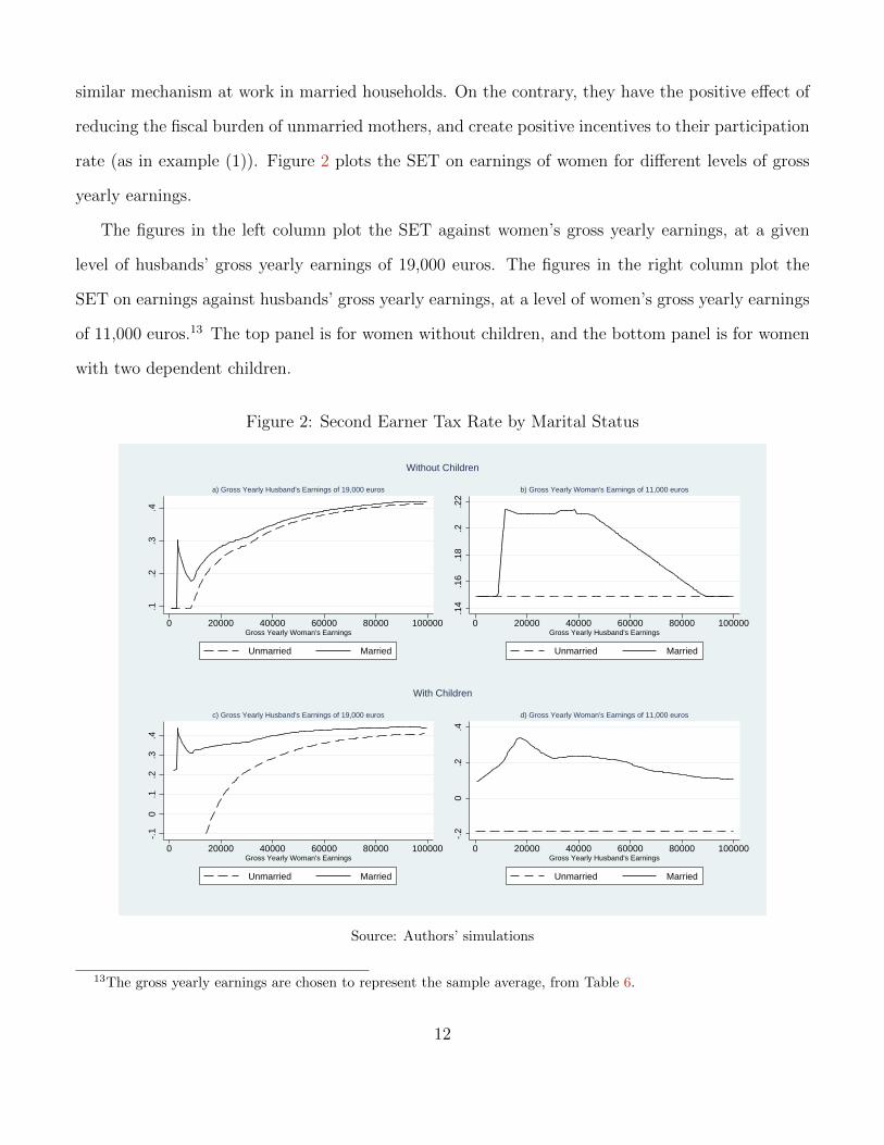
rate (as in example (1)). Figure 2 plots the SET on earnings of women for different levels of gross

yearly earnings.

The figures in the left column plot the SET against women’s gross yearly earnings, at a given

level of husbands’ gross yearly earnings of 19,000 euros. The figures in the right column plot the

SET on earnings against husbands’ gross yearly earnings, at a level of women’s gross yearly earnings

of 11,000 euros.13 The top panel is for women without children, and the bottom panel is for women

with two dependent children.

Figure 2: Second Earner Tax Rate by Marital Status

.1.2

.3.4

0 20000 40000 60000 80000 100000Gross Yearly Woman's Earnings

Unmarried Married

a) Gross Yearly Husband's Earnings of 19,000 euros

.14

.16

.18

.2.2

2

0 20000 40000 60000 80000 100000Gross Yearly Husband's Earnings

Unmarried Married

b) Gross Yearly Woman's Earnings of 11,000 euros

Without Children

-.1

0.1

.2.3

.4


Unmarried Married

c) Gross Yearly Husband's Earnings of 19,000 euros

-.2

0.2

.4


Unmarried Married

d) Gross Yearly Woman's Earnings of 11,000 euros

With Children

Source: Authors’ simulations

13The gross yearly earnings are chosen to represent the sample average, from Table 6.

12

In panel a), we can see that the married-unmarried difference in SET is particularly relevant for

low women’s earnings (less than 4, 000 euros), and dies down as the income increases. The pick of the

SET of married women occurs in correspondence of yearly earnings of about 3, 500 euros. At that

point, husbands are not entitled to receive a tax credit for dependent spouse, and the SET jumps

from 9 to about 30 percent. These couples face a trade-off between having the wife participating in

the labor market earning a very low salary and not receiving tax credits (but still increasing the total

household income), versus not participating and paying lower taxes (because of the tax credits).

In panel b), the SET of married women is constant and equal to the one of unmarried women,

until a level of husband’s income of about 8,000 euros. In the interval [0, 8, 000] euros, the husband’s

income belongs to the no-tax area, and only his wife’s earnings are subject to taxation. After that

point, both incomes are taxed and the SET increases to about 20 percent. It is worth noting that

the SET remains high for medium levels of household incomes, to decrease and reach the second

earner tax rate of unmarried women for husbands’ earnings in the highest percentiles.

In panel c) and d), we plot the SET of households with children. We can see that (low earnings)

unmarried mothers are subject to negative taxation, as they are eligible to universal cash transfers

for dependent children, which are higher than the amount of taxes that they are supposed to pay.

Married mothers are subject to a higher SET because of the (lower) amount of universal cash

transfers for dependent children agreed to the husband. The SET reaches a pick of 44 percent for

wife’s earnings of about 3, 200 euros. As in panel a), the difference between the tax paid by married

and unmarried women decreases with their earnings. In panel d), we can see more clearly the impact

of the universal cash transfers for dependent children. The SET of married mothers is increasing

up to yearly gross husband’s earnings of about 19,000 euros. After that point, the decreasing cash

transfers for dependent children and spouse diminish the difference between taxes to pay if working

or not working.

Now, we take a closer look at the impact of taxes by marital status (Figure 3, panel a) and b)).

In panel a), we observe that unmarried women with children have a SET which is much lower than

that of unmarried women without children, as the former receive cash transfers for the dependent

13

children. On the contrary, for married women (panel b)), the presence of children negatively affects

the second earner tax rate. Panel c) plots the difference of SET between married and unmarried

women by presence of children, against their yearly earnings. The difference is significatively positive

for low-income mothers whose husbands are entitled to receive tax credits and transfers. But it is

very close to zero for higher incomes and, in general, for childless women.

Figure 3: Second Earner Tax Rate by Marital Status and Presence of Children

-.1

0.1

.2.3

.4.5


w/o children w/children

a) Unmarried Women

-.1

0.1

.2.3

.4.5



b) Married Women

0.5

11.

52

2.5

0 20000 40000 60000 80000 100000Gross Yearly Wife's Income


c) Second Earner Tax Rate - Difference (Married - Unmarried)


In summary, the Italian tax system, even if based on individuals and not on households, generates

a set of negative incentives to female labor force participation. This is due to universal cash transfers

and tax credits for dependent children and spouse that increase the second earner tax rate of married

relative to unmarried women. The distortion is increasing in the number of children, and reaches

a maximum at a level of husband’s gross yearly earnings of about 8, 000 euros for childless couples,

14

and 19, 000 euros for couples with children.

Having discussed the empirical features that motivate our work, we present, in the next section,

the model and the results of the estimations.

3 Estimation and Results

3.1 The Model and the Empirical Specification

In our dataset (EU-SILC) each individual is observed for at most four years, not generating enough

variation to provide a robust estimation of a dynamic model. We therefore rely on a simple static

model, assuming that yearly wages are a sufficient statistic for the life cycle earnings profile.

We build a two-stage static model of female labor supply. In the first stage, a woman decides

whether to join the labor market and search for a job. If she does, she enters the second stage and

receives, for each possible amount of working time h ∈ H ⊂ <+, a job offer characterized by a level

of gross yearly earnings wf (h). She can accept one of them or reject them all and stay unemployed

(h = 0). We assume that the household preferences are described by a stochastic utility function

Umar(h,D(·), Z), where D denotes the household disposable income, and Z is a set of exogenous

characteristics. The superscript mar is an indicator of the marital status of the woman, and the

utility function is allowed to be different for married and unmarried women.

The complex structure of the tax system implies that the disposable income is a function of the

total household income, and on the household composition. Extensively, the disposable income can

be computed as

D = wf (h) + wm + y − T (wf (h), wm,mar, chi), (2)

where T (·) denotes net transfers from the government, given by the difference between taxes and

benefits; wm is the husband gross earnings (which is 0 if the woman is not married); y is the household

gross income from other (non-labor) sources; mar and chi are the marital status and the number

15

of dependent children, respectively. As the paper’s focus is on female labor supply, both wm(h) and

y are taken as given as in Kleven et al. [2009]. Implicitly, we assume a negligible elasticity of male

labor supply.

We solve the problem by backward induction, starting from stage 2. A woman in the labor

market will maximize utility

V mar(wm, y, Z) = maxh

Umar(h,D(wf (h), wm, y,mar, chi), Z). (3)

In the second stage, a woman faces a trade-off between the utility from non working (enjoying leisure

and carrying out domestic work) and working, augmenting the disposable income of the household.

In stage 1, she decides whether or not to enter the labor market. To make her choice, she

compares the utility from not participating and the expected utility from entering the labor market.

The problem is the following:

max{Umar(0, D(0, wm, y,mar, chi), Z), E [V mar(wm, y, Z)]− c}, (4)

where c is the cost of entering the labor market, and E [V (wm, y, Z)] is the expected utility generated

by the maximization problem in stage 2. We assume a quadratic utility function

Umar(h,D(·), Z) = αmarh + βmarD + βmar

2 D2 + γmarh Z + εmar

h . (5)

Notice that the marginal utility of income depends on marital status. Moreover, the effect of all the

other variables included in Z varies with both mar and h.

The difference (αmarh −αmar

0 )+(γmarh −γmar

0 )Z captures the disutility of working (utility of leisure)

of an amount of time h. Finally, εmarh is a stochastic error component. We know that, if ε is i.i.d.

according to a type I extreme value distribution, the probability of observing a woman in the labor

16

market, opting for a choice h = k is

Prk = Pr(h = k) =eU

mar(k,D(wf (k),wm,y,mar,chi),Z)∑h e

Umar(h,D(wf (h),wm,y,mar,chi),Z)). (6)

Similarly, the probability of being in the labor market is

Pr(s = 1) =eE[V (wm,y,Z)]−c

eUmar(0,D(0,wm,y,mar,chi),Z) + eE[V (wm,y,Z)]−c , (7)

where s indicates the labor market status. Finally, for a given observation sample {zi}i∈I =

{wmi, wfi(hi), yi, hi, Zi}i∈I , we can compute the log-likelihood function:

L({zi}i∈I) =∑i

{(1− si) [log(1− Pr(si = 1))] + si

[log(Pr(si = 1)) +

∑k

1k(hi) log(Pr(h = k))

]}(8)

where 1k(hi) is a binary variable which equals 1 if individual i chooses h = k and 0 otherwise. The

coefficients are in Tables 12 and 13.

3.2 The Data

We use micro data from the EU-SILC, the Community Statistics on Income and Living Conditions.

The survey collects information relating to a broad range of issues in relation to income and living

conditions. SILC is conducted by the Statistics Offices of the European countries involved in the

project on an annual basis, in order to monitor changes in income and living conditions over time.

Every person aged 16 years and over in a household is required to participate to the survey. Two

different types of questions are asked in the household survey: household questions, and personal

questions. The former covers details of accommodation and facilities together with regular household

expenses (mortgage repayments, etc.). This information is supplied by the Head of the Household.

The latter covers details of items such as work, income and health, and are obtained from every

household member aged 16 years and over. We combine household and personal information to

construct a data set which contains information on the spouse of the interviewed household member.

17

We focus on the cross-sectional information of the years 2007 and 2008, because they are the last

two years available of EU-SILC after a few changes in the tax system that took place from 2006 to

2007.14 We restrict the sample to women aged 26-54 years, to avoid the modeling of schooling and

retirement decisions. Moreover, we exclude self-employed men and women, and individuals that are

coded as disabled or unfitted to work. Descriptive statistics are in Table 6 in the Appendix.

The data set provides information on gross labor income of all members of the household (wm,wf ),

and total household income. By difference it is possible to compute the non-labor income (y).

Nevertheless, it is necessary to compute the potential income for all possible labor supply choices

h ∈ H, including the non-employed. To correct for selection bias, a two-stage non-linear procedure

is adopted which differs in few features from the standard Heckman correction.

Let’s consider a standard Mincerian equation

log(wf |X) = βX + µ+ ε, (9)

where X is a vector of observed characteristics, µ is an individual characteristic component (e.g.

skill or ability), and ε is a specific job component. It is well known that if either µ or ε are correlated

with the probability of observing wf , simple least squares estimation are biased. In particular, wages

are observed only if the worker decides to (i) enter the labor market, and (ii) accept a given job offer.

Both choices are presumably affected by µ or ε. Workers with high ability (µ) are more likely to

enter the labor market, and to accept better offers (high ε). Let s = 1 and e = 1 denote the events

of a worker being in the labor market and employed, respectively. A worker enters the labor market,

i.e. s = 1, if (γsX + us) > 0. Next, he accepts a job offer, i.e. s = 1 and e = 1, if (γeX + ue) > 0.

Observed earnings can be expressed as

E(log(wf )|X, s = 1, e = 1) = βX + E(µ|X, s = 1) + E(ε|X, s = 1, e = 1). (10)

14EU-SILC provides two types of data: (1) cross-sectional data pertaining to a given time or a certain time periodwith variables on income, poverty, social exclusion and other living conditions; (2) longitudinal data pertaining toindividual-level changes over time, observed periodically over a four years period.

18

Since the dataset does not provide us with a strong instrument, we perform a non-linear selection

procedure with

E(µ|s = 1, e = 1) = E(µ|s = 1) = f(Pr(s = 1|X)) (11)

E(ε|s = 1, e = 1) = g(Pr(e = 1|s = 1, X), P r(s = 1|X)), (12)

where f(·) and g(·, ·) are generic functions.

In the first stage, the propensity scores q(X) = Pr(s = 1|X), p(X) = Pr(e = 1|s = 1, X) are

estimated by a standard probit procedure, with variables X including: age, dummy variables for

geographical regions, presence of dependent children, education, and net income from other sources

(both husbands income, if any, and non-labor income). Moreover, we distinguish between married

and unmarried women. The marginal effects obtained from the probit regressions are in Tables 9

and 10 in the Appendix.

In the second stage, we estimate the wage equation assuming that both f(·) and g(·, ·) are step

functions, constant within decile intervals, and report the coefficients in Table 11 in the Appendix.

We use the residuals of the wage equation estimation to compute the predicted wages. Finally,

we assume three possible levels of labor supply, h ∈ [0, 1, 2], denoting respectively unemployment,

part-time and full-time employment.

3.3 Estimation Results

The model is estimated allowing the parameters to differ between married and unmarried women.

That is, we allow the elasticity of the labor force participation to change with the marital status. We

include several variables that affect the decision to participate in the labor market, as age, education

level, years of past work experience, and presence of children.

Panel b) of Figure 4 plots the estimated participation rates by age, and marital status. Comparing

it to the data in panel a), we can observe that the model generates the levels and the decreasing

trend of the participation rate of the different subgroups of women.

19

Figure 4: Labor Force Participation of Italian Women by Age

0.40

0.50

0.60

0.70

0.80

0.90

1.00

26 30 34 38 42 46 50 54Age

All Unmarried w\children

Married w\children All w/o children

a) Data

0.40

0.50

0.60

0.70

0.80

0.90

1.00

26 30 34 38 42 46 50 54Age

All Unmarried w\children

Married w\children All w/o children

b) Model


Even thought the taxation system is not age-dependent, the age of women is correlated with

their own earnings, their husband’s earnings, and the number of children. As we described above,

all of these elements affect the tax burden, and hence, the labor decision of second earners.

Figure 5: Results by Education Level - Data vs Model

0.524 0.524

0.760 0.760

0.884 0.884

0.2

.4.6

.8

< Secondary School Secondary School > Secondary School

Labor Force Participation Rate

Data Model

0.492 0.490

0.734 0.734

0.863 0.862

0.2

.4.6

.8


Employment Rate

Data Model


The model replicates the percentage of women in the labor force, and the percentage of women

20

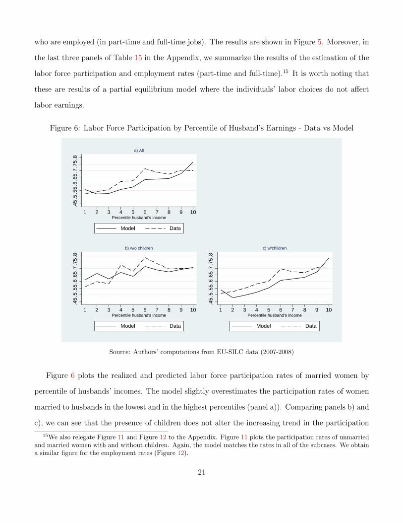
who are employed (in part-time and full-time jobs). The results are shown in Figure 5. Moreover, in

the last three panels of Table 15 in the Appendix, we summarize the results of the estimation of the

labor force participation and employment rates (part-time and full-time).15 It is worth noting that

these are results of a partial equilibrium model where the individuals’ labor choices do not affect

labor earnings.

Figure 6: Labor Force Participation by Percentile of Husband’s Earnings - Data vs Model

.45

.5.5

5.6

.65

.7.7

5.8

1 2 3 4 5 6 7 8 9 10Percentile husband's income

Model Data

a) All

.45

.5.5

5.6

.65

.7.7

5.8


Model Data

b) w/o children

.45

.5.5

5.6

.65

.7.7

5.8


Model Data

c) w/children


Figure 6 plots the realized and predicted labor force participation rates of married women by

percentile of husbands’ incomes. The model slightly overestimates the participation rates of women

married to husbands in the lowest and in the highest percentiles (panel a)). Comparing panels b) and

c), we can see that the presence of children does not alter the increasing trend in the participation

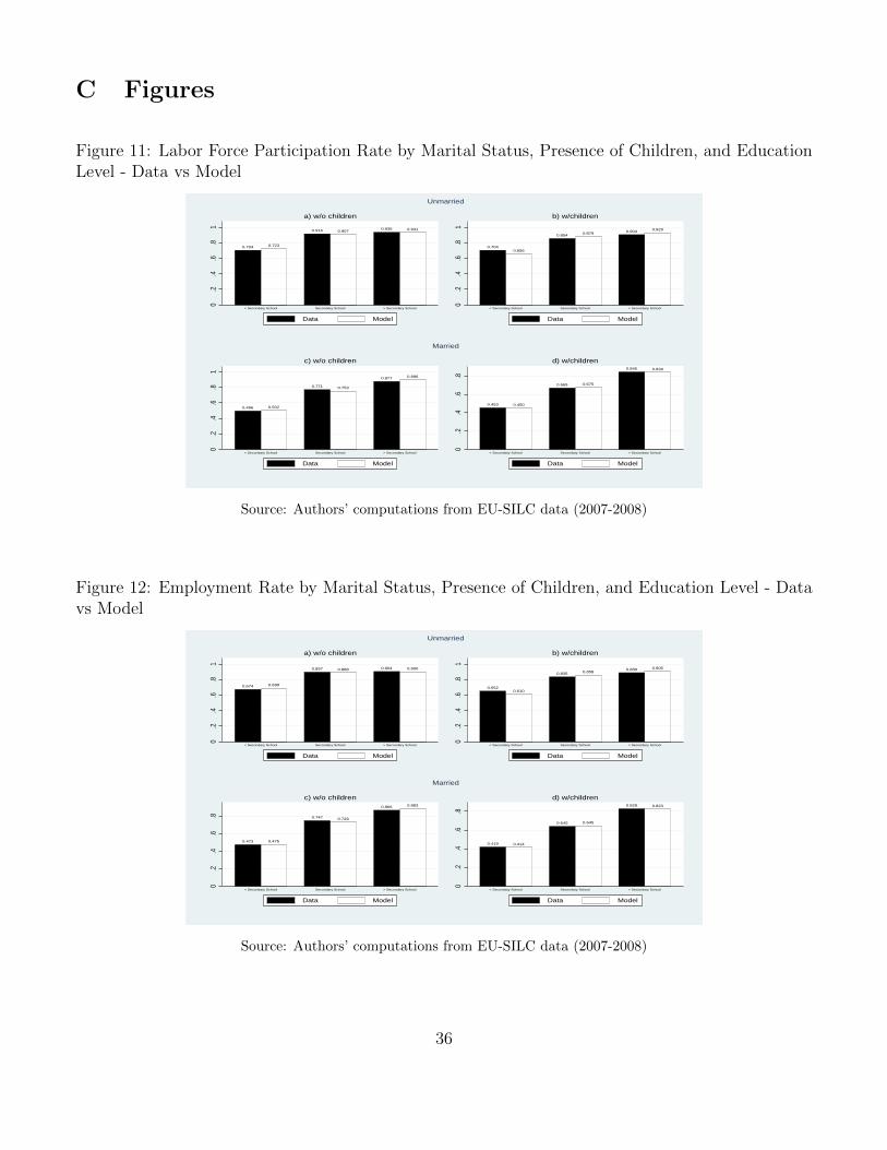
15We also relegate Figure 11 and Figure 12 to the Appendix. Figure 11 plots the participation rates of unmarriedand married women with and without children. Again, the model matches the rates in all of the subcases. We obtaina similar figure for the employment rates (Figure 12).

21

rates. The distortion takes place regardless of the presence of children. Childless households may

still be eligible to receive tax credits for dependent spouse, increasing the amount of their SET.

4 Alternative Taxation Systems

The reform of the taxation system has been a topic of several discussions in the Italian government.

In this section, we use the parameters obtained from the estimation of the model to simulate the

labor force participation rate and the employment rate under four different taxation systems that

have been considered in the political and academic debate.

That is: the joint taxation, the working tax credit, the gender-based taxation, and a mixture of

individual (or Italian) and joint tax system. In Table 14 in the Appendix, we summarize the main

characteristics of these alternative systems.

An important issue involved in our tax simulation exercises is that, when different tax units and

tax systems are considered, the total tax revenue might change. We analyze what happens to the

amount of tax paid by a household in the case of constant total tax revenue. Constant tax revenue

is achieved by increasing each household tax by a constant amount.16 The results of the simulations

are in Table 15 that can be found in the Appendix.

Moreover, we compute several measures of poverty to compare the effects on the well-being of

individuals for each of the taxation system that we consider.

4.1 Joint Family Taxation

The joint taxation system is currently implemented in Portugal, France and Germany. It provides

tax advantages to large families with low income as the average tax rate decreases with the number

of household components. As shown by some existing literature,17 this system creates a system of

16A simulation that does not take this into account shows that the joint tax system implies a revenue loss of about18%; the working tax credit of about 2%; the gender-based system of about 11%.

17See Buffeteau and Echevin [2003] for France, Steiner and Wrohlich [2004] for Germany, and Aassve et al. [2007]for Italy.

22

negative incentives to participation for both of the spouses, and especially for women.

We simulate a taxation system similar to the one we find in France, where the gross income is

the household income divided by the number of parts (the quotient familial, a coefficients which

increases with the number of household components).

Let ym and yf be the gross yearly incomes of the two spouses, q be quotient familial, and t(·)

be the tax schedule. Then, the amount of tax is equal to qt((ym + yf )/q) instead of t(ym) + t(yf ).

In the simulation, we drop all tax credits for dependent spouse and universal cash transfers. The

quotient familial is assumed to equal the number of household components.

This tax system implies an increase in the average tax rate from 17 to 19 percent, and a 15

percent increase in the SET. The increase concerns all marital status, regardless of the presence of

children (Table 15 in the Appendix).

Participation and employment rates decrease by about 3 percentage points. Under this system,

unmarried women do not change their behavior significantly. Married women are the most negatively

affected. In particular, married women without children decrease their participation rate by 5

percentage points, and married women with children decrease it by 6 percentage points.

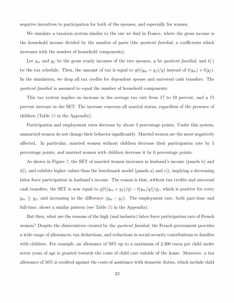
As shown in Figure 7, the SET of married women increases in husband’s income (panels b) and

d)), and exhibits higher values than the benchmark model (panels a) and c)), implying a decreasing

labor force participation in husband’s income. The reason is that, without tax credits and universal

cash transfers, the SET is now equal to q[t((ym + yf )/q) − t(ym/q)]/yf , which is positive for every

ym ≥ yf , and increasing in the difference (ym − yf ). The employment rate, both part-time and

full-time, shows a similar pattern (see Table 15 in the Appendix).

But then, what are the reasons of the high (and inelastic) labor force participation rate of French

women? Despite the disincentives created by the quotient familial, the French government provides

a wide range of allowances, tax deductions, and reductions in social security contributions to families

with children. For example, an allowance of 50% up to a maximum of 2,300 euros per child under

seven years of age is granted towards the costs of child care outside of the home. Moreover, a tax

allowance of 50% is credited against the costs of assistance with domestic duties, which include child

23

care.

Figure 7: Second Earner Tax Rate by Marital Status and Presence of Children - Joint Taxation.1

.2.3

.4.5


Unmarried Unmarried, Joint Tax

Married Married, Joint Tax


.1.2

.3.4

.5





Without Children

-.1

0.1

.2.3

.4





-.2

0.2

.4





With Children


To these fiscal measures, we should add the widespread system of day-care centers (both individ-

ual and collective) for children both younger and older than three years of age; monetary transfers

to parents who decide to exit the labor to take care of the children; and, a system of primary schools

that offers overtime assistance to children with parents at work.18 This set of services (other than

fiscal) provide incentives to low income French mothers to enter (or to remain) in the labor force

participation. In Italy the disincentives created by the fiscal system are not offset by any other

family policy aimed to reduce the burden of the child care cost.

18See Adema and Thevenon [2008] for a discussion of the existing policies directed to French families.

24

4.2 The Working Tax Credit

The American Earned Income Tax Credit (EITC) and the British Working Tax Credit (WTC) are

two systems of negative taxation. The tax unit is the individual. Based on them, households where

both of the spouses are employed, have the right to receive a tax credit which is increasing in the

size of the family and which can even become a transfer.19 Chote et al. [2007] provide evidence of an

increase from 45 to 55 percent in employment rates of unmarried mothers in Great Britain. Eissa

and Liebman [1996] and Ellwood [2000] obtain similar results for the EITC.

We assume that individual working tax credits amount to 1, 840 euros, regardless of the individual

or household income. Moreover, we eliminate the tax credits for dependent spouse and we set the

universal cash transfers to 137 euros a month for the first child and 121 euros a month for the

following children, regardless of the total household income.20 This proposition is in line with the

tax system of several European countries, and the suggestions of Atkinson [2011] and Levy et al.

[2007].

This system provides incentives to married women, especially when they have children. The

model forecasts an increase in participation and employment rates of about 3 percentage points.

There is no change for unmarried women. Contrary to the Italian system, the working tax credit

has all of the characteristics of an individual taxation system. In fact, tax credits or transfers (and

hence, second earner tax rates) do not depend on the spouse’s income, and hence does not vary with

the marital status.

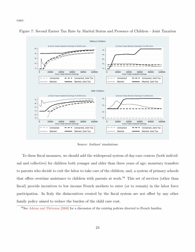
This is shown in Figure 8, panels b) and d), where the SET is constant at about 15 percent,

and independent of the marriage. Similarly, panels a) and c) show that the SET changes only

with women’s income. Another interesting features of this system is that it provides incentives to

undertake low earnings jobs. As we can see in Figure 8 (panels a) and c)), the SET is particularly

low (and even negative) at low levels of earnings. Additionally, as reported in Table 15, the working

19For example, in the WTC, households with two parents working at least 16 hours a week can obtain a reim-bursement of 80 percent of the child care costs.

20We assume that the transfers for the first and second child are equal to the maximum amount of transfersguaranteed by the Italian tax system in the two cases.

25

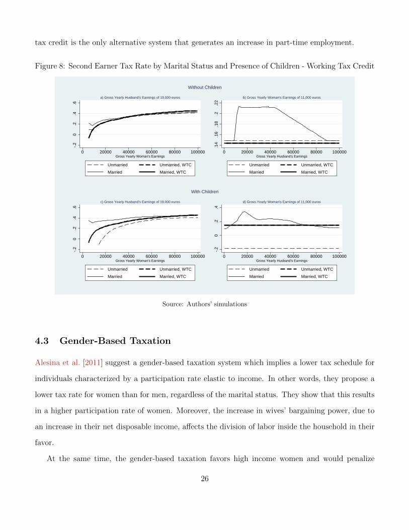
tax credit is the only alternative system that generates an increase in part-time employment.

Figure 8: Second Earner Tax Rate by Marital Status and Presence of Children - Working Tax Credit-.

20

.2.4

.6


Unmarried Unmarried, WTC

Married Married, WTC


.14

.16

.18

.2.2

2





Without Children

-.2

0.2

.4.6





-.2

0.2

.4





With Children


4.3 Gender-Based Taxation

Alesina et al. [2011] suggest a gender-based taxation system which implies a lower tax schedule for

individuals characterized by a participation rate elastic to income. In other words, they propose a

lower tax rate for women than for men, regardless of the marital status. They show that this results

in a higher participation rate of women. Moreover, the increase in wives’ bargaining power, due to

an increase in their net disposable income, affects the division of labor inside the household in their

favor.

At the same time, the gender-based taxation favors high income women and would penalize

26

low income men. Furthermore, it would imply an equal treatment of two single parent families

identical in income but different in the gender of the parents. Saint-Paul [2007] underlines that

there is not reason to believe that participation rate of women is always more elastic than that of

men. For example, single women, with and without children, do not behave differently than men.

Alternatively, Saint-Paul [2007] suggest to apply a lower tax rate to supplemental hours worked,

regardless of the gender.

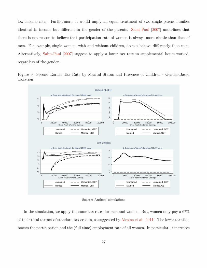
Figure 9: Second Earner Tax Rate by Marital Status and Presence of Children - Gender-BasedTaxation

.1.2

.3.4


Unmarried Unmarried, GBT

Married Married, GBT


.14

.16

.18

.2.2

2





Without Children

-.1

0.1

.2.3

.4





-.2

0.2

.4





With Children


In the simulation, we apply the same tax rates for men and women. But, women only pay a 67%

of their total tax net of standard tax credits, as suggested by Alesina et al. [2011]. The lower taxation

boosts the participation and the (full-time) employment rate of all women. In particular, it increases

27

both participation and (full-time) employment rates by more than 2 percentage points, regardless of

the marital status and the number of children. However, the tax credits for dependent spouse and

cash transfers continue to generate the positive correlation between labor force participation and

husband’s income.

From Figure 9, we can see that this system leads to a decrease in the SET of every woman, even

thought it maintains a relatively high SET of low-income married women (as we did not change the

system of tax credits and universal cash transfers).

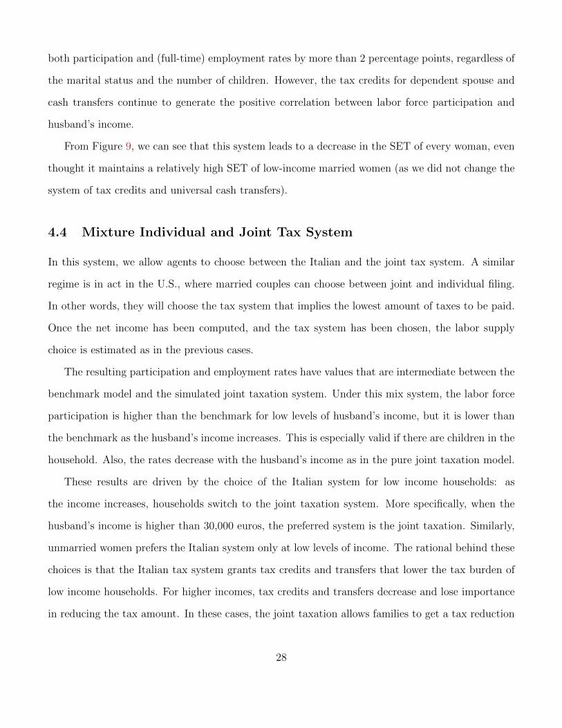
4.4 Mixture Individual and Joint Tax System

In this system, we allow agents to choose between the Italian and the joint tax system. A similar

regime is in act in the U.S., where married couples can choose between joint and individual filing.

In other words, they will choose the tax system that implies the lowest amount of taxes to be paid.

Once the net income has been computed, and the tax system has been chosen, the labor supply

choice is estimated as in the previous cases.

The resulting participation and employment rates have values that are intermediate between the

benchmark model and the simulated joint taxation system. Under this mix system, the labor force

participation is higher than the benchmark for low levels of husband’s income, but it is lower than

the benchmark as the husband’s income increases. This is especially valid if there are children in the

household. Also, the rates decrease with the husband’s income as in the pure joint taxation model.

These results are driven by the choice of the Italian system for low income households: as

the income increases, households switch to the joint taxation system. More specifically, when the

husband’s income is higher than 30,000 euros, the preferred system is the joint taxation. Similarly,

unmarried women prefers the Italian system only at low levels of income. The rational behind these

choices is that the Italian tax system grants tax credits and transfers that lower the tax burden of

low income households. For higher incomes, tax credits and transfers decrease and lose importance

in reducing the tax amount. In these cases, the joint taxation allows families to get a tax reduction

28

through the quotient familial, a tool which is independent of income. This explains the switch from

the benchmark to the joint system at medium-high levels of household income.

In panels b) and d) of Figure 10, we can see that the SET of married women is still increasing

in husband’s income (as in the joint taxation system). In panel a), the SET of married women

is slightly higher than the benchmark only for incomes lower than 10,000 euros. In panel c), we

observe that the SET of married mothers behaves closely to the Italian system. Moreover, the SET

of unmarried women is lower than the benchmark only if they have children.

Figure 10: Second Earner Tax Rate by Marital Status and Presence of Children - Mixture Taxation

.1.2

.3.4

.5

0 20000 40000 60000 80000 100000Gross Yearly Woman’s Income

Unmarried Unmarried, Mixture

Married Married, Mixture

a) Gross Yearly Husband’s Income of 19,000 euros

.1.1

5.2

.25

.3.3

5

0 20000 40000 60000 80000 100000Gross Yearly Husband’s Income



b) Gross Yearly Woman’s Income of 11,000 euros

Without Children

−.1

0.1

.2.3

.4

0 20000 40000 60000 80000 100000Gross Yearly Woman’s Income



c) Gross Yearly Husband’s Income of 19,000 euros

−.2

0.2

.4

0 20000 40000 60000 80000 100000Gross Yearly Husband’s Income



d) Gross Yearly Woman’s Income of 11,000 euros

With Children


29

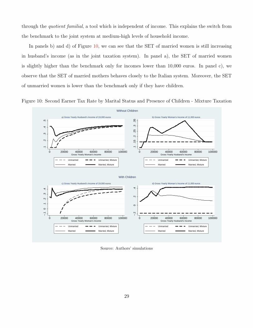
4.5 Welfare Implications

In order to evaluate the welfare effects of the estimated and simulated tax systems, we compute

several measures of poverty. In general, the tax system has a pervasive impact on poverty, both

directly through its role in the distribution of society’s resources, and indirectly through its effects

on the incentives for economic decisions like working and saving. We decide to focus on poverty

measures as we think that the impact of tax reform on low-income families is especially important

in light of the persistence of poverty, wage stagnation at the bottom, and the growth of income

inequality. Our choice is also motivated by the last report of the National Institute of Statistics of

Italy (Istat [2009]), which documents an increase in the poverty incidence among the households

with a worker as reference person.21

In our computations, we define yi(j) as the equivalised disposable income of individual i in house-

hold j, that is the total income of a household, after tax and other deductions, which is available for

spending or saving, divided by the number of household members converted into equalised adults.22

The poverty measures are defined as follows:

(1) Head count index: it measures the proportion of the population for whom income is below

the poverty line.23 Let s(j) be the number of members of household j and P the poverty line.

Then, the head count index is defined as

HC =∑i

HCi =∑i

(1P (yji ) ∗ s(j)∑

j s(j)

)

where

1P (yi(j)) =

1 if yi(j) ≤ P

0 otherwise

21As we mentioned in the introduction, the reduction of the population below the poverty line is also a target ofEurope2020, the project of the European Commission.

22See http://epp.eurostat.ec.europa.eu/statistics_explained/index.php/Glossary:Equivalised_

disposable_income.23The poverty threshold is reported by Eurostat (http://epp.eurostat.ec.europa.eu/statistics_explained/

index.php/Main_Page, File: At-risk-of-poverty rate and At risk poverty threshold in the EU, 2007). In Italy, it equals9,007 euros in 2007.

30

http://epp.eurostat.ec.europa.eu/statistics_explained/index.php/Glossary:Equivalised_disposable_income

http://epp.eurostat.ec.europa.eu/statistics_explained/index.php/Glossary:Equivalised_disposable_income

http://epp.eurostat.ec.europa.eu/statistics_explained/index.php/Main_Page

http://epp.eurostat.ec.europa.eu/statistics_explained/index.php/Main_Page

The head count index has the disadvantage of ignoring the differences in well-being between

different poor individuals.

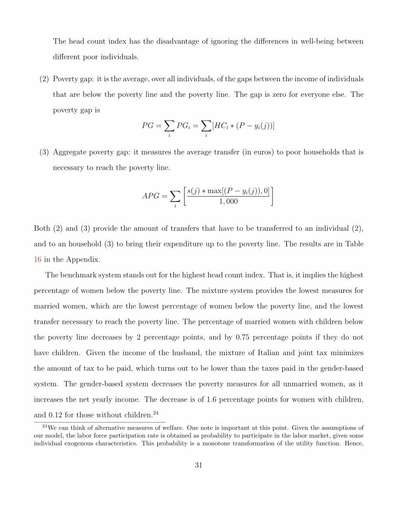
(2) Poverty gap: it is the average, over all individuals, of the gaps between the income of individuals

that are below the poverty line and the poverty line. The gap is zero for everyone else. The

poverty gap is

PG =∑i

PGi =∑i

[HCi ∗ (P − yi(j))]

(3) Aggregate poverty gap: it measures the average transfer (in euros) to poor households that is

necessary to reach the poverty line.

APG =∑i

[s(j) ∗max[(P − yi(j)), 0]

1, 000

]

Both (2) and (3) provide the amount of transfers that have to be transferred to an individual (2),

and to an household (3) to bring their expenditure up to the poverty line. The results are in Table

16 in the Appendix.

The benchmark system stands out for the highest head count index. That is, it implies the highest

percentage of women below the poverty line. The mixture system provides the lowest measures for

married women, which are the lowest percentage of women below the poverty line, and the lowest

transfer necessary to reach the poverty line. The percentage of married women with children below

the poverty line decreases by 2 percentage points, and by 0.75 percentage points if they do not

have children. Given the income of the husband, the mixture of Italian and joint tax minimizes

the amount of tax to be paid, which turns out to be lower than the taxes paid in the gender-based

system. The gender-based system decreases the poverty measures for all unmarried women, as it

increases the net yearly income. The decrease is of 1.6 percentage points for women with children,

and 0.12 for those without children.24

24We can think of alternative measures of welfare. One note is important at this point. Given the assumptions ofour model, the labor force participation rate is obtained as probability to participate in the labor market, given someindividual exogenous characteristics. This probability is a monotone transformation of the utility function. Hence,

31

5 Conclusions

In this paper, we have used micro data from EU-SILC to estimate a structural model of female labor

supply. In particular, men’s labor supply and incomes are given, and women decide, in two stages,

whether to search for an occupation, and to accept it or not.

We show that the model matches the low level of the Italian labor force participation and employ-

ment rates, and replicates the positive correlation between wife’s participation rate and husband’s

yearly income. Moreover, we show that the Italian individual taxation system generates disincentives

to women labor supply, especially when married with children. This is due to a set of tax credits

for dependent spouse and children, and universal cash transfers for children that increases the fiscal

burden of low income households, and the second earner tax rate of women married to low income

or unemployed men.

We then use the estimated parameters to measure the behavioral effects of alternative tax sys-

tems: joint family taxation, a system inspired by the British working tax credit, the gender-based

taxation, and a mixture of the Italian and joint taxation system. We show that the first implies a

substantial drop in the participation rate of married women. The working tax credit and the gender-

based tax systems boost the participation rate, with the effects of the former being concentrated on

unskilled and low educated women. Unsurprisingly, the mixture system generates a set of results

that combines those of the Italian and the joint tax systems. The participation rate is higher than

that produced by the joint tax rate but lower than the benchmark. Moreover, it generates a negative

correlation between the participation rate and the husband’s income, as in the joint tax system.

Overall, the results of the simulations show that moving towards a system of tax credits in line

with the British or the American ones, would reduce the fiscal burden of low earnings workers,

mostly married women. Cash transfers that are independent of the total household income would

reduce the disincentives to work created by the Italian taxation system. We could also expect that

providing incentives to low income jobs would decrease the incentives of taking up irregular jobs.

changes in participation rates reflect the directions of changes in welfare, as computed directly from the model.

32

Appendix

A Details of the Italian Tax System

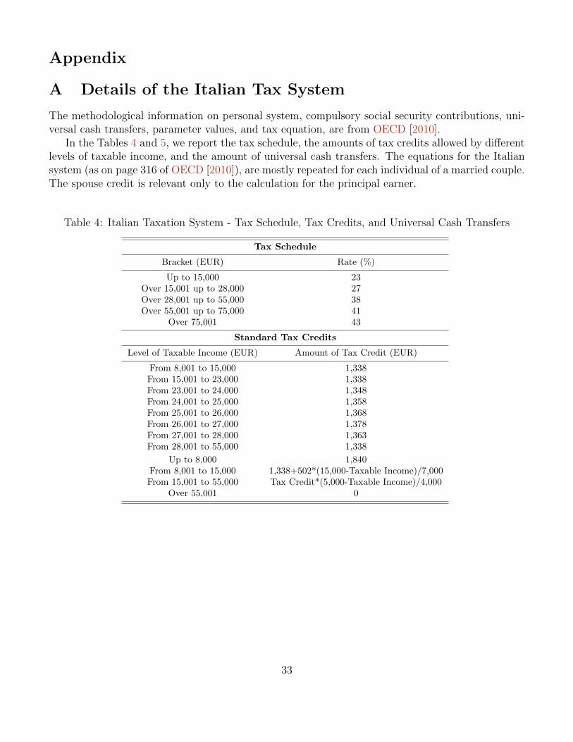
The methodological information on personal system, compulsory social security contributions, uni-versal cash transfers, parameter values, and tax equation, are from OECD [2010].

In the Tables 4 and 5, we report the tax schedule, the amounts of tax credits allowed by differentlevels of taxable income, and the amount of universal cash transfers. The equations for the Italiansystem (as on page 316 of OECD [2010]), are mostly repeated for each individual of a married couple.The spouse credit is relevant only to the calculation for the principal earner.

Table 4: Italian Taxation System - Tax Schedule, Tax Credits, and Universal Cash Transfers

Tax Schedule

Bracket (EUR) Rate (%)

Up to 15,000 23Over 15,001 up to 28,000 27Over 28,001 up to 55,000 38Over 55,001 up to 75,000 41

Over 75,001 43

Standard Tax Credits

Level of Taxable Income (EUR) Amount of Tax Credit (EUR)

From 8,001 to 15,000 1,338From 15,001 to 23,000 1,338From 23,001 to 24,000 1,348From 24,001 to 25,000 1,358From 25,001 to 26,000 1,368From 26,001 to 27,000 1,378From 27,001 to 28,000 1,363From 28,001 to 55,000 1,338

Up to 8,000 1,840From 8,001 to 15,000 1,338+502*(15,000-Taxable Income)/7,000From 15,001 to 55,000 Tax Credit*(5,000-Taxable Income)/4,000

Over 55,001 0

33

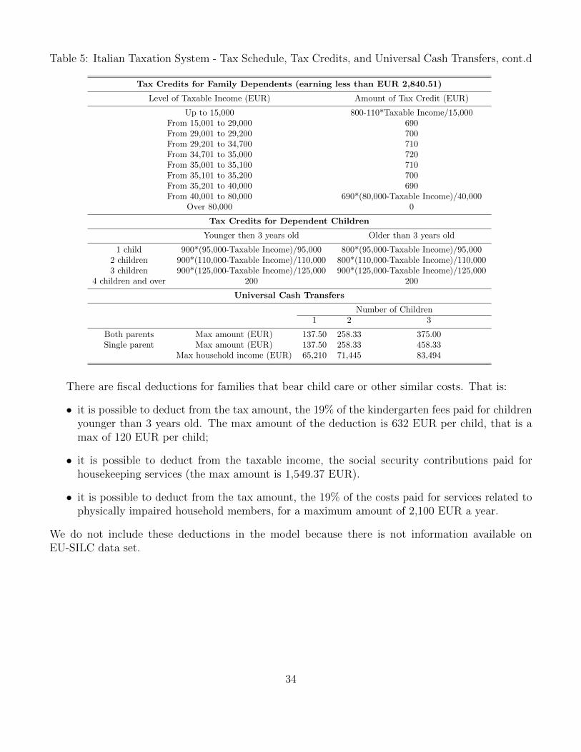
Table 5: Italian Taxation System - Tax Schedule, Tax Credits, and Universal Cash Transfers, cont.d

Tax Credits for Family Dependents (earning less than EUR 2,840.51)

Level of Taxable Income (EUR) Amount of Tax Credit (EUR)

Up to 15,000 800-110*Taxable Income/15,000From 15,001 to 29,000 690From 29,001 to 29,200 700From 29,201 to 34,700 710From 34,701 to 35,000 720From 35,001 to 35,100 710From 35,101 to 35,200 700From 35,201 to 40,000 690From 40,001 to 80,000 690*(80,000-Taxable Income)/40,000

Over 80,000 0

Tax Credits for Dependent Children

Younger then 3 years old Older than 3 years old

1 child 900*(95,000-Taxable Income)/95,000 800*(95,000-Taxable Income)/95,0002 children 900*(110,000-Taxable Income)/110,000 800*(110,000-Taxable Income)/110,0003 children 900*(125,000-Taxable Income)/125,000 900*(125,000-Taxable Income)/125,000

4 children and over 200 200

Universal Cash Transfers

Number of Children1 2 3

Both parents Max amount (EUR) 137.50 258.33 375.00Single parent Max amount (EUR) 137.50 258.33 458.33

Max household income (EUR) 65,210 71,445 83,494

There are fiscal deductions for families that bear child care or other similar costs. That is:

• it is possible to deduct from the tax amount, the 19% of the kindergarten fees paid for childrenyounger than 3 years old. The max amount of the deduction is 632 EUR per child, that is amax of 120 EUR per child;

• it is possible to deduct from the taxable income, the social security contributions paid forhousekeeping services (the max amount is 1,549.37 EUR).

• it is possible to deduct from the tax amount, the 19% of the costs paid for services related tophysically impaired household members, for a maximum amount of 2,100 EUR a year.

We do not include these deductions in the model because there is not information available onEU-SILC data set.

34

B Summary Statistics

Table 6: Descriptive statistics, EU-SILC 2007-2008

Variable WomenUnmarried Married

Mean Std.dev. Mean Std.dev.

Number of observation 5,926 13,081Age 38.47 8.19 42.30 7.15With children (%) 24.23 73.29

Activity Rate (%) 84.37 63.42Experience (years) 18.12 10.47 23.37 9.78Unemployment Rate (%) 2.73 2.65Incidence of Part-time (%) 13.96 15.73Average annual earnings (euros) 14,054.90 13,373.15 10,312.30 12,829.53Household Non-Labor Income (euros) 22,931.56 30,769.47 9,928.55 16,516.17Average husband’s earnings (euros) 19,611.62 19,150.48

RegionNorth-West 25.19 21.19North-East 25.51 23.72Center 24.81 23.88South 18.24 22.67Islands 6.24 8.53

Education<Secondary Education 28.23 39.62Secondary Education 41.14 39.56> Secondary Education 30.63 20.82

35

C Figures

Figure 11: Labor Force Participation Rate by Marital Status, Presence of Children, and EducationLevel - Data vs Model

0.704 0.723

0.916 0.9070.936 0.931

0.2

.4.6

.81


a) w/o children

Data Model

0.7040.656

0.854 0.879 0.904 0.929

0.2

.4.6

.81


b) w/children

Data Model

Unmarried

0.496 0.502

0.771 0.753

0.877 0.896

0.2

.4.6

.81


c) w/o children

Data Model

0.453 0.450

0.669 0.675

0.845 0.839

0.2

.4.6

.8< Secondary School Secondary School > Secondary School

d) w/children

Data Model

Married


Figure 12: Employment Rate by Marital Status, Presence of Children, and Education Level - Datavs Model

0.674 0.689

0.897 0.888 0.904 0.900

0.2

.4.6

.81


a) w/o children

Data Model

0.6520.610

0.835 0.8580.889 0.905

0.2

.4.6

.81


b) w/children

Data Model

Unmarried

0.473 0.475

0.747 0.729

0.866 0.883

0.2

.4.6

.8


c) w/o children

Data Model

0.419 0.414

0.640 0.645

0.828 0.823

0.2

.4.6

.8


d) w/children

Data Model

Married


36

D Tables

Table 7: Probit - Coefficients

Y = 1 (in labor force) Italy France Spain UK Germany

Husband’s Earnings 1.29e-06* -3.88e06** 2.09e-07 -2.21e-06*** -5.42e-06***(6.67e-07) (1.60e-06) (1.01e-06) (4.64e-07) (6.50e-07)

Household Non-Labor Income -2.13e-06*** -0.000*** -5.05e-06*** -7.31e-06*** -0.000***(5.47e-07) (1.72e-06) (1.15e-06) (7.99e-07) (1.05e-06)

Married -0.763*** -0.372*** -0.682*** -0.330*** -0.315***(0.073) (0.164) (0.088) (0.058) (0.112)

Employed Husband 0.190*** 0.178 -0.002 0.614*** -0.141(0.071) (0.166) (0.086) (0.054) (0.112)

Children -0.243*** -0.312*** -0.165*** -0.493*** -0.532***(0.026) (0.164) (0.033) (0.041) (0.038)

Age 0.054*** 0.050 0.010 0.092*** 0.130***(0.016) (0.038) (0.021) (0.025) (0.024)

Age2 -0.001*** -0.000 -0.000 -0.001*** -0.001***(0.000) (0.000) (0.000) (0.000) (0.000)

Education:

Secondary Education 0.609*** 0.561*** 0.405*** 0.788*** 0.390***(0.031) (0.060) (0.034) (0.052) (0.057)

> Secondary Education 1.046*** 1.072*** 0.952*** 1.079*** 0.711***(0.030) (0.075) (0.035) (0.057) (0.058)




Table 8: Probit - Marginal Effects

Y = 1 (in labor force) Italy France Spain UK Germany

Husband’s Earnings 4.21e-07* -7.49e-07** 5.54e-08 -5.52e-07*** -1.23e-06***(2.17e-07) (3.09e-07) (2.68e-07) (1.16e-07) (1.48e-07)

Household Non-Labor Income -6.94e-07*** -2.70e-06*** -1.34e-06*** -1.82e-06*** -2.37e-06***(1.78e-07) (3.31e-07) (3.06e-07) (1.99e-07) (2.37e-07)

Married -0.224*** -0.069*** -0.164*** -0.080*** -0.068***(0.019) (0.029) (0.019) (0.013) (0.023)

Employed Husband 0.063*** 0.035 -0.006 0.152*** -0.031(0.024) (0.033) (0.023) (0.013) (0.024)

Children -0.078*** -0.056*** -0.043*** -0.118*** -0.115***(0.008) (0.011) (0.009) (0.009) (0.008)

Age 0.018*** 0.009 0.003 0.023*** 0.029***(0.005) (0.007) (0.006) (0.006) (0.005)

Age2 -0.000*** -0.000 -0.000 -0.000*** -0.000***(0.000) (0.000) (0.000) (0.000) (0.000)

Education:

Secondary Education 0.189*** 0.104*** 0.097*** 0.201*** 0.086***(0.007) (0.011) (0.007) (0.013) (0.012)

> Secondary Education 0.274*** 0.174*** 0.224*** 0.231*** 0.161***(0.006) (0.010) (0.007) (0.011) (0.013)




37

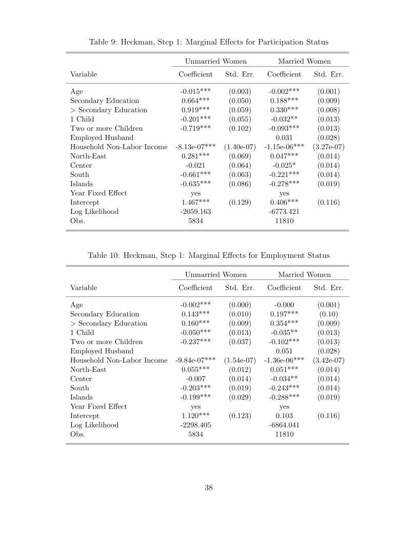
Table 9: Heckman, Step 1: Marginal Effects for Participation Status

Unmarried Women Married Women

Variable Coefficient Std. Err. Coefficient Std. Err.

Age -0.015*** (0.003) -0.002*** (0.001)Secondary Education 0.664*** (0.050) 0.188*** (0.009)> Secondary Education 0.919*** (0.059) 0.330*** (0.008)1 Child -0.201*** (0.055) -0.032** (0.013)Two or more Children -0.719*** (0.102) -0.093*** (0.013)Employed Husband 0.031 (0.028)Household Non-Labor Income -8.13e-07*** (1.40e-07) -1.15e-06*** (3.27e-07)North-East 0.281*** (0.069) 0.047*** (0.014)Center -0.021 (0.064) -0.025* (0.014)South -0.661*** (0.063) -0.221*** (0.014)Islands -0.635*** (0.086) -0.278*** (0.019)Year Fixed Effect yes yesIntercept 1.467*** (0.129) 0.406*** (0.116)Log Likelihood -2059.163 -6773.421Obs. 5834 11810

Table 10: Heckman, Step 1: Marginal Effects for Employment Status



Age -0.002*** (0.000) -0.000 (0.001)Secondary Education 0.143*** (0.010) 0.197*** (0.10)> Secondary Education 0.160*** (0.009) 0.354*** (0.009)1 Child -0.050*** (0.013) -0.035** (0.013)Two or more Children -0.237*** (0.037) -0.102*** (0.013)Employed Husband 0.051 (0.028)Household Non-Labor Income -9.84e-07*** (1.54e-07) -1.36e-06*** (3.42e-07)North-East 0.055*** (0.012) 0.051*** (0.014)Center -0.007 (0.014) -0.034** (0.014)South -0.203*** (0.019) -0.243*** (0.014)Islands -0.199*** (0.029) -0.288*** (0.019)Year Fixed Effect yes yesIntercept 1.120*** (0.123) 0.103 (0.116)Log Likelihood -2298.405 -6864.041Obs. 5834 11810

38

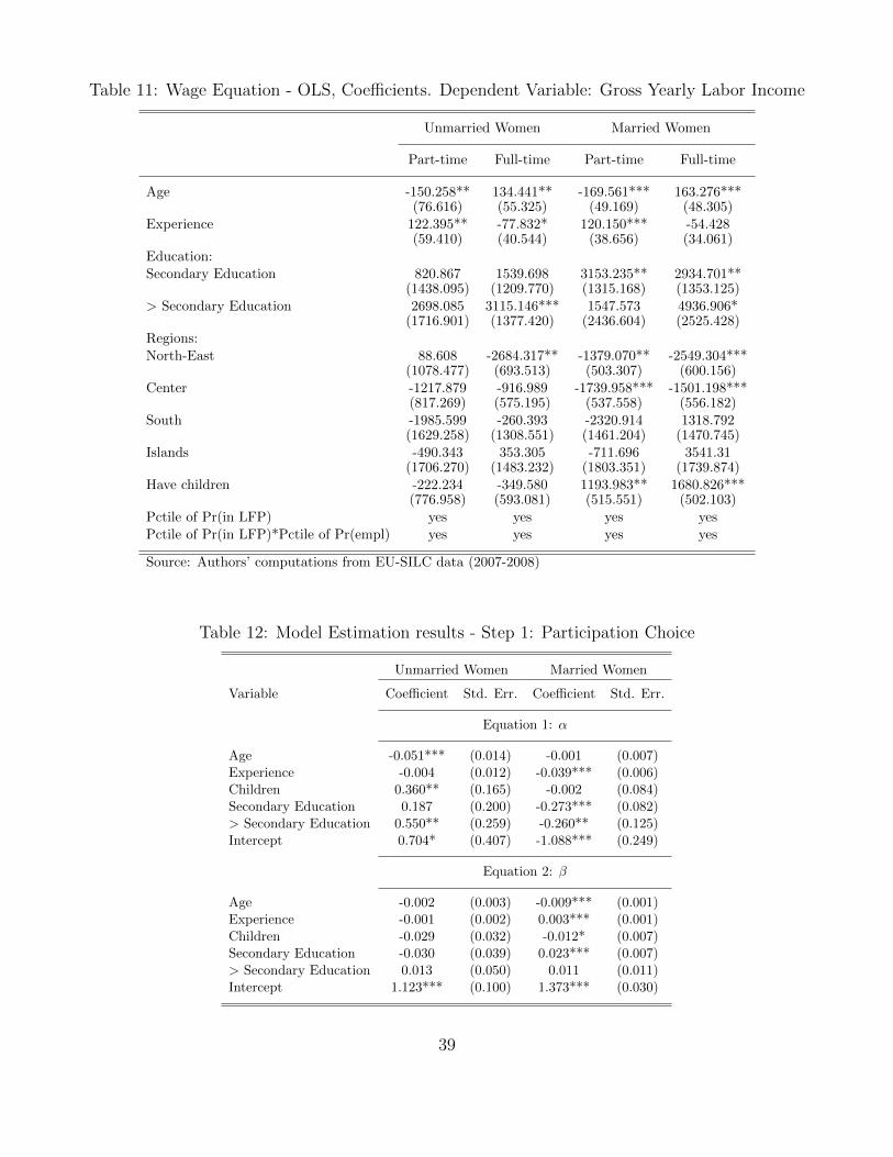
Table 11: Wage Equation - OLS, Coefficients. Dependent Variable: Gross Yearly Labor Income


Part-time Full-time Part-time Full-time

Age -150.258** 134.441** -169.561*** 163.276***(76.616) (55.325) (49.169) (48.305)

Experience 122.395** -77.832* 120.150*** -54.428(59.410) (40.544) (38.656) (34.061)

Education:Secondary Education 820.867 1539.698 3153.235** 2934.701**

(1438.095) (1209.770) (1315.168) (1353.125)> Secondary Education 2698.085 3115.146*** 1547.573 4936.906*

(1716.901) (1377.420) (2436.604) (2525.428)Regions:North-East 88.608 -2684.317** -1379.070** -2549.304***

(1078.477) (693.513) (503.307) (600.156)Center -1217.879 -916.989 -1739.958*** -1501.198***

(817.269) (575.195) (537.558) (556.182)South -1985.599 -260.393 -2320.914 1318.792

(1629.258) (1308.551) (1461.204) (1470.745)Islands -490.343 353.305 -711.696 3541.31

(1706.270) (1483.232) (1803.351) (1739.874)Have children -222.234 -349.580 1193.983** 1680.826***

(776.958) (593.081) (515.551) (502.103)Pctile of Pr(in LFP) yes yes yes yesPctile of Pr(in LFP)*Pctile of Pr(empl) yes yes yes yes


Table 12: Model Estimation results - Step 1: Participation Choice



Equation 1: α

Age -0.051*** (0.014) -0.001 (0.007)Experience -0.004 (0.012) -0.039*** (0.006)Children 0.360** (0.165) -0.002 (0.084)Secondary Education 0.187 (0.200) -0.273*** (0.082)> Secondary Education 0.550** (0.259) -0.260** (0.125)Intercept 0.704* (0.407) -1.088*** (0.249)

Equation 2: β

Age -0.002 (0.003) -0.009*** (0.001)Experience -0.001 (0.002) 0.003*** (0.001)Children -0.029 (0.032) -0.012* (0.007)Secondary Education -0.030 (0.039) 0.023*** (0.007)> Secondary Education 0.013 (0.050) 0.011 (0.011)Intercept 1.123*** (0.100) 1.373*** (0.030)

39

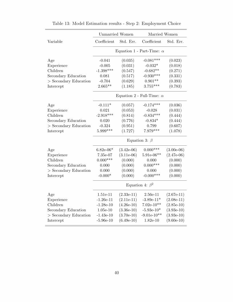
Table 13: Model Estimation results - Step 2: Employment Choice



Equation 1 - Part-Time: α

Age -0.041 (0.035) -0.081*** (0.023)Experience -0.005 (0.031) -0.032* (0.018)Children -1.398*** (0.547) -0.682** (0.271)Secondary Education 0.081 (0.517) -0.930*** (0.331)> Secondary Education -0.704 (0.629) 0.901** (0.393)Intercept 2.665** (1.185) 3.755*** (0.783)

Equation 2 - Full-Time: α

Age -0.111* (0.057) -0.174*** (0.036)Experience 0.021 (0.053) -0.028 (0.031)Children -2.918*** (0.814) -0.834*** (0.444)Secondary Education 0.020 (0.776) -0.834* (0.444)> Secondary Education -0.324 (0.951) 0.799 (0.607)Intercept 5.999*** (1.727) 7.979*** (1.078)

Equation 3: β

Age 6.82e-06* (3.42e-06) 0.000*** (3.00e-06)Experience 7.35e-07 (3.11e-06) 5.91e-06** (2.47e-06)Children 0.000*** (0.000) 0.000 (0.000)Secondary Education 0.000 (0.000) 0.000*** (0.000)> Secondary Education 0.000 (0.000) 0.000 (0.000)Intercept -0.000* (0.000) -0.000*** (0.000)

Equation 4: β2

Age 1.51e-11 (2.33e-11) 2.56e-11 (2.67e-11)Experience -1.26e-11 (2.11e-11) -3.89e-11* (2.08e-11)Children -1.28e-10 (4.26e-10) 7.02e-10** (2.85e-10)Secondary Education 1.05e-10 (3.36e-10) -5.93e-10* (3.93e-10)> Secondary Education -1.43e-10 (3.70e-10) -9.01e-10** (3.93e-10)Intercept -5.96e-10 (6.49e-10) 1.82e-10 (9.60e-10)

40

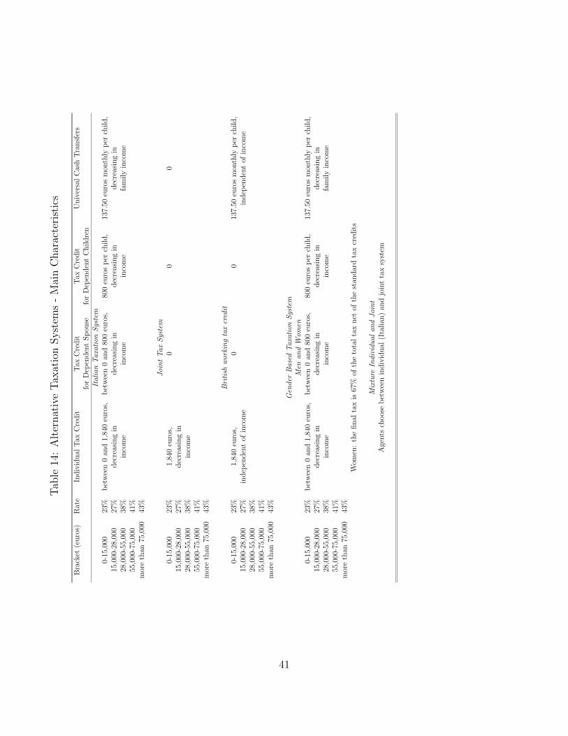
Tab

le14

:A

lter

nat

ive

Tax

atio

nSyst

ems

-M

ain

Char

acte

rist

ics

Bra

cket

(euro

s)R

ate

Indiv

idual

Tax

Cre

dit

Tax

Cre

dit

Tax

Cre

dit

Univ

ersa

lC

ash

Tra

nsf

ers

for

Dep

enden

tSp

ouse

for

Dep

enden

tC

hildre

nIt

alia

nT

axat

ion

Sys

tem

0-15

,000

23%

bet

wee

n0

and

1,84

0eu

ros,

bet

wee

n0

and

800

euro

s,80

0eu

ros

per

child,

137.

50eu

ros

mon

thly

per

child,

15,0

00-2

8,00

027

%dec

reas

ing

indec

reas

ing

indec

reas

ing

indec

reas

ing

in28

,000

-55,

000

38%

inco

me

inco

me

inco

me

fam

ily

inco

me

55,0

00-7

5,00

041

%m

ore

than

75,0

0043

%

Joi

nt

Tax

Sys

tem

0-15

,000

23%

1,84

0eu

ros,

00

015

,000

-28,

000

27%

dec

reas

ing

in28

,000

-55,

000

38%

inco

me

55,0

00-7

5,00

041

%m

ore

than

75,0

0043

%

Bri

tish

wor

kin

gta

xcr

edit

0-15

,000

23%

1,84

0eu

ros,

00

137.

50eu

ros

mon

thly

per

child,

15,0

00-2

8,00

027

%in

dep

enden

tof

inco

me

indep

enden

tof

inco

me

28,0

00-5

5,00

038

%55

,000

-75,

000

41%

mor

eth

an75

,000

43%

Gen

der

Bas

edT

axat

ion

Sys

tem

Men

and

Wom

en0-

15,0

0023

%b

etw

een

0an

d1,

840

euro

s,b

etw

een

0an

d80

0eu

ros,

800

euro

sp

erch

ild,

137.

50eu

ros

mon

thly

per

child,

15,0

00-2

8,00

027

%dec

reas

ing

indec

reas

ing

indec

reas

ing

indec

reas

ing

in28

,000

-55,

000

38%

inco

me

inco

me

inco

me

fam

ily

inco

me

55,0

00-7

5,00

041

%m

ore

than

75,0

0043

%W

omen

:th

efinal

tax

is67

%of

the

tota

lta

xnet

ofth

est

andar

dta

xcr

edit

s

Mix

ture

Indi

vidu

alan

dJ

oin

tA

gents

choos

eb

etw

een

indiv

idual

(Ita

lian

)an

djo

int

tax

syst

em

41

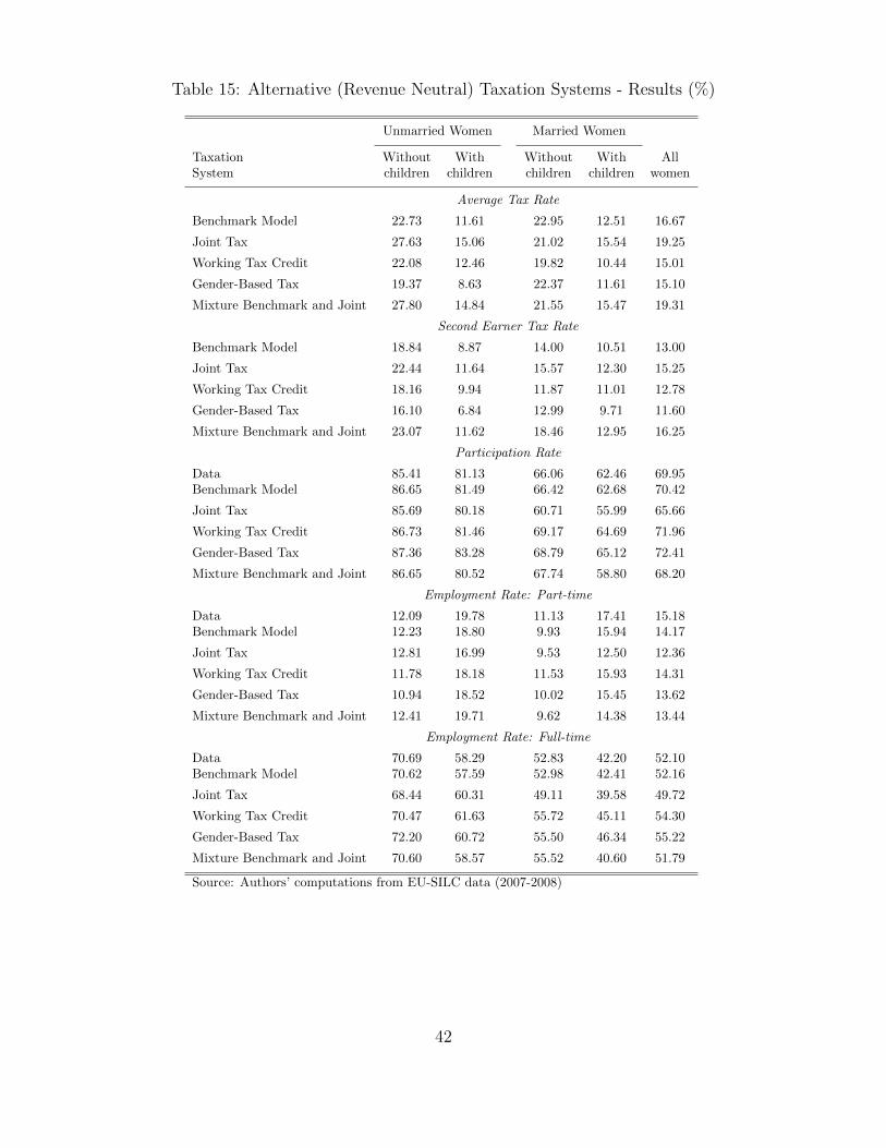
Table 15: Alternative (Revenue Neutral) Taxation Systems - Results (%)


Taxation Without With Without With AllSystem children children children children women

Average Tax Rate

Benchmark Model 22.73 11.61 22.95 12.51 16.67

Joint Tax 27.63 15.06 21.02 15.54 19.25

Working Tax Credit 22.08 12.46 19.82 10.44 15.01

Gender-Based Tax 19.37 8.63 22.37 11.61 15.10

Mixture Benchmark and Joint 27.80 14.84 21.55 15.47 19.31

Second Earner Tax Rate

Benchmark Model 18.84 8.87 14.00 10.51 13.00

Joint Tax 22.44 11.64 15.57 12.30 15.25


Gender-Based Tax 16.10 6.84 12.99 9.71 11.60


Participation Rate

Data 85.41 81.13 66.06 62.46 69.95Benchmark Model 86.65 81.49 66.42 62.68 70.42

Joint Tax 85.69 80.18 60.71 55.99 65.66


Gender-Based Tax 87.36 83.28 68.79 65.12 72.41


Employment Rate: Part-time


Joint Tax 12.81 16.99 9.53 12.50 12.36


Gender-Based Tax 10.94 18.52 10.02 15.45 13.62


Employment Rate: Full-time


Joint Tax 68.44 60.31 49.11 39.58 49.72


Gender-Based Tax 72.20 60.72 55.50 46.34 55.22



42

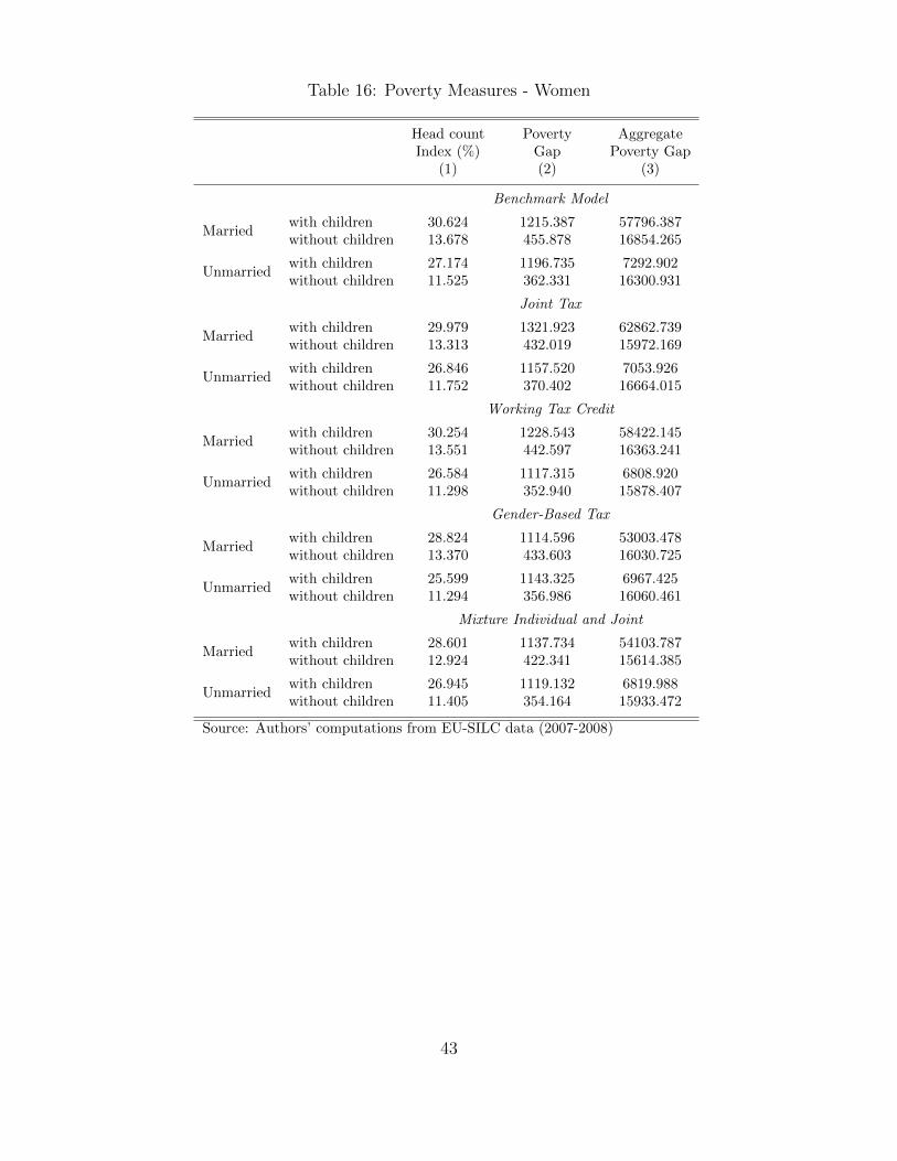
Table 16: Poverty Measures - Women

Head count Poverty AggregateIndex (%) Gap Poverty Gap

(1) (2) (3)

Benchmark Model

Marriedwith children 30.624 1215.387 57796.387without children 13.678 455.878 16854.265

Unmarriedwith children 27.174 1196.735 7292.902without children 11.525 362.331 16300.931

Joint Tax



Working Tax Credit



Gender-Based Tax



Mixture Individual and Joint




43

AcknowledgementsWe would like to thank the participants to the Applied Economics Lunch Seminar at the Paris

School of Economics, the lunch seminar at THEMA (Universite de Cergy-Pontoise), several pre-sentations at the Bank of Italy, Ugo Colombino, Nezih Guner, Andrea Ichino, Julien Prat, PaolaProfeta, and the members of the Committee in charge of awarding the prize in memoriam of EttaChiuri (2011). All errors are ours.

References

Aassve, A., Pazienza, M., Rapallini, C., 2007. Does Italy Need Family Income Taxation? WorkingPapers 77. ECINEQ, Society for the Study of Economic Inequality.

Adema, W. and Thevenon O., 2008. Les Politiques de Conciliation du Travail et de la Vie Familialeen France au Regard des Pays de l’OCDE. Recherches et Previsions Septembre, 93, 51 – 72.

Alesina, A., Ichino, A., Karabarbounis, L., 2011. Gender-Based Taxation and the Division of FamilyChores. American Economic Journal: Economic Policy 3(2), 1–40.

Atkinson, A., 2011. The Case for Universal Child Benefit, in: Walker, A., Sinfield, A., Walker, C.(Eds.), Fighting Poverty, Inequality and Social Injustice. A Manifesto Inspired by Peter Townsend.Bristol, Policy Press.

Bar, M., Leukhina, O., 2009. To Work or Not to Work: Did Tax Reforms Affect Labor ForceParticipation of Married Couples? The B.E. Journal of Macroeconomics 9.

Blundell, R., Bozio, A., Laroque, G., 2011. Extensive and Intensive Margins of Labour Supply:Working Hours in the US, UK and France. IFS Working Papers W11/01. Institute for FiscalStudies.

Blundell, R., Duncan, A., McCrae, J., Meghir, C., 2000. The Labour Market Impact of the WorkingFamilies’ Tax Credit. Fiscal Studies 21, 75–103.

Blundell, R., Hoynes, H., 2003. Has “In-Work” Benefit Reform Helped the Labour Market?, in:Card, D., Blundell, R., Freeman, R. (Eds.), Seeking a Premiere Economy: The Economic Effectsof British Economic Reforms, 1980-2000. The University of Chicago Press.

Buffeteau, S., Echevin, D., 2003. Taxation, Marriage and Labor Supply: Evidence From a NaturalExperiment in France. Cahiers de recherche 340. CIRPEE.

Burtless, G., Hausman, J., 1978. The Effect of Taxation on Labor Supply: Evaluating the “Gary”Negative Income Tax Experiments. Journal of Political Economy 86, 1103–30.

Cavalli, M., Fiorio, C.V., 2006. Individual vs Family Taxation: An Analysis Using tabeita04. SSRNeLibrary .

Chote, R., Emmerson, C., Leicester, A., Miles, D., 2007. The IFS Green Budget: January 2007.Technical Report.

44

Colombino, U., Del Boca, D., 1990. The Effect of Taxes on Labor Supply in Italy. Journal of HumanResources 25, 390–414.

Colombino, U., Strøm, S., Aaberge, R., 2000. Labor Supply Responses and Welfare Effects FromReplacing Current Tax Rules by a Flat Tax: Empirical Evidence From Italy, Norway and Sweden.Journal of Population Economics 13, 595–621.

Davis, S., Henrekson, M., 2004. Tax Effects on Work Activity, Industry Mix and Shadow EconomySize: Evidence from Rich-Country Comparisons. NBER Working Papers 10509. National Bureauof Economic Research, Inc.

Eissa, N., Liebman, J.B., 1996. Labor Supply Response to the Earned Income Tax Credit. TheQuarterly Journal of Economics 111, 605–37.

Ellwood, D., 2000. The Impact of the Earned Income Tax Credit and Social Policy Reforms onWork, Marriage, and Living Arrangements. National Tax Journal 53, 1165–86.

Fang, H., Keane, M., 2004. Assessing the Impact of Welfare Reform on Single Mothers. BrookingsPapers on Economic Activity 35, 1–116.

Hausman, J., 1980. The Effect of Wages, Taxes, and Fixed Costs on Women’s Labor Force Partici-pation. Journal of Public Economics 14, 161–194.

Hausman, J., 1985. Chapter 4 Taxes and Labor Supply, in: Auerbach, A., Feldstein, M. (Eds.),Handbook of Public Economics. Elsevier. volume 1, pp. 213–263.

Immervoll, H., Kleven, H.J., Kreiner, C.T., Saez, E., 2007. Welfare Reform in European Countries:A Microsimulation Analysis. Economic Journal 117, 1–44.

Istat, 2009. Poverty in Italy. Technical Report. Istat.

Kleven, H.J., Kreiner, C.T., Saez, E., 2009. The Optimal Income Taxation of Couples. Econometrica77,2, 537-560.

Levy, H., Lietz, C., Sutherland, H., 2007. A Guaranteed Income for Europe’s Children, in: Jenkins,S., Micklewright, J. (Eds.), Inequality and Poverty Re-Examined. Oxford University Press.

Manning, A., Petrongolo, B., 2008. The Part-Time Pay Penalty for Women in Britain. EconomicJournal 118, F28–F51.

Meyer, B., Rosenbaum, D., 2001. Welfare, the Earned Income Tax Credit, and the Labor Supply ofSingle Mothers. The Quarterly Journal of Economics 116, 1063–1114.

Mooij, R., 2008. Reinventing the Dutch Tax-Benefit System: Exploring the Frontier of the Equity-Efficiency Trade-Off. International Tax and Public Finance 15, 87–103.

OECD, 2010. Taxing Wages 2008-2009. Special Feature: Non-Tax Compulsory Payments as anAdditional Burden on Labour Income. OECD.

45

Olovsson, C., 2009. Why Do Europeans Work So Little? International Economic Review 50, 39–61.

Prescott, E., 2004. Why Do Americans Work So Much More Than Europeans? Quarterly Review,Federal Reserve Bank of Minneapolis, 2–13.

Rogerson, R., 2006. Understanding Differences in Hours Worked. Review of Economic Dynamics 9,365 – 409.

Saez, E., 2002. Optimal Income Transfer Programs: Intensive Versus Extensive Labor SupplyResponses. The Quarterly Journal of Economics 117, 1039–1073.

Saint-Jaques, G., 2009. Individualization of Taxes and Tanfers and the Labor Supply Decision ofWomen: Simulating the Current French System and Possible Reforms. Masters Dissertation. Ecolenormale superieure.

Saint-Paul, G., 2007. Against “Gender-Based Taxation”. CEPR Discussion Papers 6582. C.E.P.R.Discussion Papers.

Steiner, V., Wrohlich, K., 2004. Household Taxation, Income Splitting and Labor Supply Incentives:A Microsimulation Study for Germany. Discussion Papers of DIW Berlin 421. DIW Berlin, GermanInstitute for Economic Research.

46

Documents

Fabrizio Colonna, Stefania Marcassa To cite this version