Embed Size (px)
Citation preview

Extrema of Functions of Two Variables
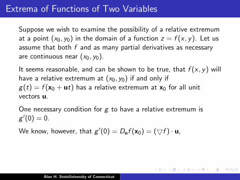
Suppose we wish to examine the possibility of a relative extremumat a point (x0, y0) in the domain of a function z = f (x , y).
Let usassume that both f and as many partial derivatives as necessaryare continuous near (x0, y0).
It seems reasonable, and can be shown to be true, that f (x , y) willhave a relative extremum at (x0, y0) if and only ifg(t) = f (x0 + ut) has a relative extremum at x0 for all unitvectors u.
One necessary condition for g to have a relative extremum isg ′(0) = 0.
We know, however, that g ′(0) = Duf (x0) = (5f ) · u, and (5f ) · ucan equal 0 for all unit vectors u if and only if both partialderivatives of f are 0.
Such points are called critical points or stationary points.
Alan H. SteinUniversity of Connecticut

Extrema of Functions of Two Variables
Suppose we wish to examine the possibility of a relative extremumat a point (x0, y0) in the domain of a function z = f (x , y). Let usassume that both f and as many partial derivatives as necessaryare continuous near (x0, y0).
It seems reasonable,
and can be shown to be true, that f (x , y) willhave a relative extremum at (x0, y0) if and only ifg(t) = f (x0 + ut) has a relative extremum at x0 for all unitvectors u.
One necessary condition for g to have a relative extremum isg ′(0) = 0.
We know, however, that g ′(0) = Duf (x0) = (5f ) · u, and (5f ) · ucan equal 0 for all unit vectors u if and only if both partialderivatives of f are 0.
Such points are called critical points or stationary points.
Alan H. SteinUniversity of Connecticut
Extrema of Functions of Two Variables
Suppose we wish to examine the possibility of a relative extremumat a point (x0, y0) in the domain of a function z = f (x , y). Let usassume that both f and as many partial derivatives as necessaryare continuous near (x0, y0).
It seems reasonable, and can be shown to be true,
that f (x , y) willhave a relative extremum at (x0, y0) if and only ifg(t) = f (x0 + ut) has a relative extremum at x0 for all unitvectors u.
One necessary condition for g to have a relative extremum isg ′(0) = 0.
We know, however, that g ′(0) = Duf (x0) = (5f ) · u, and (5f ) · ucan equal 0 for all unit vectors u if and only if both partialderivatives of f are 0.
Such points are called critical points or stationary points.
Alan H. SteinUniversity of Connecticut

Extrema of Functions of Two Variables
Suppose we wish to examine the possibility of a relative extremumat a point (x0, y0) in the domain of a function z = f (x , y). Let usassume that both f and as many partial derivatives as necessaryare continuous near (x0, y0).
It seems reasonable, and can be shown to be true, that f (x , y) willhave a relative extremum at (x0, y0) if and only ifg(t) = f (x0 + ut) has a relative extremum at x0 for all unitvectors u.
One necessary condition for g to have a relative extremum isg ′(0) = 0.
We know, however, that g ′(0) = Duf (x0) = (5f ) · u, and (5f ) · ucan equal 0 for all unit vectors u if and only if both partialderivatives of f are 0.
Such points are called critical points or stationary points.
Alan H. SteinUniversity of Connecticut
Extrema of Functions of Two Variables
Suppose we wish to examine the possibility of a relative extremumat a point (x0, y0) in the domain of a function z = f (x , y). Let usassume that both f and as many partial derivatives as necessaryare continuous near (x0, y0).
It seems reasonable, and can be shown to be true, that f (x , y) willhave a relative extremum at (x0, y0) if and only ifg(t) = f (x0 + ut) has a relative extremum at x0 for all unitvectors u.
One necessary condition for g to have a relative extremum isg ′(0) = 0.
We know, however, that g ′(0) = Duf (x0) = (5f ) · u,
and (5f ) · ucan equal 0 for all unit vectors u if and only if both partialderivatives of f are 0.
Such points are called critical points or stationary points.
Alan H. SteinUniversity of Connecticut

Extrema of Functions of Two Variables
Suppose we wish to examine the possibility of a relative extremumat a point (x0, y0) in the domain of a function z = f (x , y). Let usassume that both f and as many partial derivatives as necessaryare continuous near (x0, y0).
It seems reasonable, and can be shown to be true, that f (x , y) willhave a relative extremum at (x0, y0) if and only ifg(t) = f (x0 + ut) has a relative extremum at x0 for all unitvectors u.
One necessary condition for g to have a relative extremum isg ′(0) = 0.
We know, however, that g ′(0) = Duf (x0) = (5f ) · u, and (5f ) · ucan equal 0 for all unit vectors u if and only if both partialderivatives of f are 0.
Such points are called critical points or stationary points.
Alan H. SteinUniversity of Connecticut

Using the Second Derivative Test
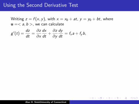
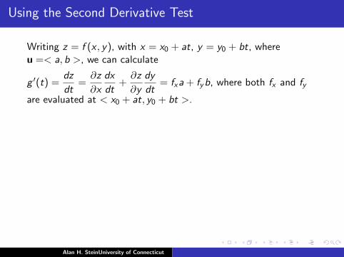
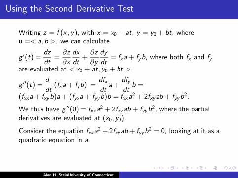
Writing z = f (x , y), with x = x0 + at, y = y0 + bt, whereu =< a, b >, we can calculate
g ′(t) =dz
dt=
∂z
∂x
dx
dt+
∂z
∂y
dy
dt= fxa + fyb, where both fx and fy
are evaluated at < x0 + at, y0 + bt >.
g ′′(t) =d
dt(fxa + fyb) =
dfxdt
a +dfydt
b =
(fxxa + fxyb)a + (fyxa + fyyb)b = fxxa2 + 2fxyab + fyyb2.
We thus have g ′′(0) = fxxa2 + 2fxyab + fyyb2, where the partial
derivatives are evaluated at (x0, y0).
Consider the equation fxxa2 + 2fxyab + fyyb2 = 0, looking at it as a
quadratic equation in a. Using the Quadratic Formula, we get
solutions a =−2fxyb ±
√(2fxyb)2 − 4fxx fyyb2
2fxx.
Alan H. SteinUniversity of Connecticut

Using the Second Derivative Test
Writing z = f (x , y), with x = x0 + at, y = y0 + bt, whereu =< a, b >, we can calculate
g ′(t) =dz
dt
=∂z
∂x
dx
dt+
∂z
∂y
dy
dt= fxa + fyb, where both fx and fy
are evaluated at < x0 + at, y0 + bt >.
g ′′(t) =d
dt(fxa + fyb) =
dfxdt
a +dfydt
b =
(fxxa + fxyb)a + (fyxa + fyyb)b = fxxa2 + 2fxyab + fyyb2.
We thus have g ′′(0) = fxxa2 + 2fxyab + fyyb2, where the partial
derivatives are evaluated at (x0, y0).
Consider the equation fxxa2 + 2fxyab + fyyb2 = 0, looking at it as a
quadratic equation in a. Using the Quadratic Formula, we get
solutions a =−2fxyb ±
√(2fxyb)2 − 4fxx fyyb2
2fxx.
Alan H. SteinUniversity of Connecticut

Using the Second Derivative Test
Writing z = f (x , y), with x = x0 + at, y = y0 + bt, whereu =< a, b >, we can calculate
g ′(t) =dz
dt=
∂z
∂x
dx
dt+
∂z
∂y
dy
dt
= fxa + fyb, where both fx and fy
are evaluated at < x0 + at, y0 + bt >.
g ′′(t) =d
dt(fxa + fyb) =
dfxdt
a +dfydt
b =
(fxxa + fxyb)a + (fyxa + fyyb)b = fxxa2 + 2fxyab + fyyb2.
We thus have g ′′(0) = fxxa2 + 2fxyab + fyyb2, where the partial
derivatives are evaluated at (x0, y0).
Consider the equation fxxa2 + 2fxyab + fyyb2 = 0, looking at it as a
quadratic equation in a. Using the Quadratic Formula, we get
solutions a =−2fxyb ±
√(2fxyb)2 − 4fxx fyyb2
2fxx.
Alan H. SteinUniversity of Connecticut
Using the Second Derivative Test
Writing z = f (x , y), with x = x0 + at, y = y0 + bt, whereu =< a, b >, we can calculate
g ′(t) =dz
dt=
∂z
∂x
dx
dt+
∂z
∂y
dy
dt= fxa + fyb,
where both fx and fy
are evaluated at < x0 + at, y0 + bt >.
g ′′(t) =d
dt(fxa + fyb) =
dfxdt
a +dfydt
b =
(fxxa + fxyb)a + (fyxa + fyyb)b = fxxa2 + 2fxyab + fyyb2.
We thus have g ′′(0) = fxxa2 + 2fxyab + fyyb2, where the partial
derivatives are evaluated at (x0, y0).
Consider the equation fxxa2 + 2fxyab + fyyb2 = 0, looking at it as a
quadratic equation in a. Using the Quadratic Formula, we get
solutions a =−2fxyb ±
√(2fxyb)2 − 4fxx fyyb2
2fxx.
Alan H. SteinUniversity of Connecticut
Using the Second Derivative Test
Writing z = f (x , y), with x = x0 + at, y = y0 + bt, whereu =< a, b >, we can calculate
g ′(t) =dz
dt=
∂z
∂x
dx
dt+
∂z
∂y
dy
dt= fxa + fyb, where both fx and fy
are evaluated at < x0 + at, y0 + bt >.
g ′′(t) =d
dt(fxa + fyb) =
dfxdt
a +dfydt
b =
(fxxa + fxyb)a + (fyxa + fyyb)b = fxxa2 + 2fxyab + fyyb2.
We thus have g ′′(0) = fxxa2 + 2fxyab + fyyb2, where the partial
derivatives are evaluated at (x0, y0).
Consider the equation fxxa2 + 2fxyab + fyyb2 = 0, looking at it as a
quadratic equation in a. Using the Quadratic Formula, we get
solutions a =−2fxyb ±
√(2fxyb)2 − 4fxx fyyb2
2fxx.
Alan H. SteinUniversity of Connecticut

Using the Second Derivative Test
Writing z = f (x , y), with x = x0 + at, y = y0 + bt, whereu =< a, b >, we can calculate
g ′(t) =dz
dt=
∂z
∂x
dx
dt+
∂z
∂y
dy
dt= fxa + fyb, where both fx and fy
are evaluated at < x0 + at, y0 + bt >.
g ′′(t) =d
dt(fxa + fyb)
=dfxdt
a +dfydt
b =
(fxxa + fxyb)a + (fyxa + fyyb)b = fxxa2 + 2fxyab + fyyb2.
We thus have g ′′(0) = fxxa2 + 2fxyab + fyyb2, where the partial
derivatives are evaluated at (x0, y0).
Consider the equation fxxa2 + 2fxyab + fyyb2 = 0, looking at it as a
quadratic equation in a. Using the Quadratic Formula, we get
solutions a =−2fxyb ±
√(2fxyb)2 − 4fxx fyyb2
2fxx.
Alan H. SteinUniversity of Connecticut

Using the Second Derivative Test
Writing z = f (x , y), with x = x0 + at, y = y0 + bt, whereu =< a, b >, we can calculate
g ′(t) =dz
dt=
∂z
∂x
dx
dt+
∂z
∂y
dy
dt= fxa + fyb, where both fx and fy
are evaluated at < x0 + at, y0 + bt >.
g ′′(t) =d
dt(fxa + fyb) =
dfxdt
a +dfydt
b
=
(fxxa + fxyb)a + (fyxa + fyyb)b = fxxa2 + 2fxyab + fyyb2.
We thus have g ′′(0) = fxxa2 + 2fxyab + fyyb2, where the partial
derivatives are evaluated at (x0, y0).
Consider the equation fxxa2 + 2fxyab + fyyb2 = 0, looking at it as a
quadratic equation in a. Using the Quadratic Formula, we get
solutions a =−2fxyb ±
√(2fxyb)2 − 4fxx fyyb2
2fxx.
Alan H. SteinUniversity of Connecticut

Using the Second Derivative Test
Writing z = f (x , y), with x = x0 + at, y = y0 + bt, whereu =< a, b >, we can calculate
g ′(t) =dz
dt=
∂z
∂x
dx
dt+
∂z
∂y
dy
dt= fxa + fyb, where both fx and fy
are evaluated at < x0 + at, y0 + bt >.
g ′′(t) =d
dt(fxa + fyb) =
dfxdt
a +dfydt
b =
(fxxa + fxyb)a + (fyxa + fyyb)b
= fxxa2 + 2fxyab + fyyb2.
We thus have g ′′(0) = fxxa2 + 2fxyab + fyyb2, where the partial
derivatives are evaluated at (x0, y0).
Consider the equation fxxa2 + 2fxyab + fyyb2 = 0, looking at it as a
quadratic equation in a. Using the Quadratic Formula, we get
solutions a =−2fxyb ±
√(2fxyb)2 − 4fxx fyyb2
2fxx.
Alan H. SteinUniversity of Connecticut

Using the Second Derivative Test
Writing z = f (x , y), with x = x0 + at, y = y0 + bt, whereu =< a, b >, we can calculate
g ′(t) =dz
dt=
∂z
∂x
dx
dt+
∂z
∂y
dy
dt= fxa + fyb, where both fx and fy
are evaluated at < x0 + at, y0 + bt >.
g ′′(t) =d
dt(fxa + fyb) =
dfxdt
a +dfydt
b =
(fxxa + fxyb)a + (fyxa + fyyb)b = fxxa2 + 2fxyab + fyyb2.
We thus have g ′′(0) = fxxa2 + 2fxyab + fyyb2, where the partial
derivatives are evaluated at (x0, y0).
Consider the equation fxxa2 + 2fxyab + fyyb2 = 0, looking at it as a
quadratic equation in a. Using the Quadratic Formula, we get
solutions a =−2fxyb ±
√(2fxyb)2 − 4fxx fyyb2
2fxx.
Alan H. SteinUniversity of Connecticut

Using the Second Derivative Test
Writing z = f (x , y), with x = x0 + at, y = y0 + bt, whereu =< a, b >, we can calculate
g ′(t) =dz
dt=
∂z
∂x
dx
dt+
∂z
∂y
dy
dt= fxa + fyb, where both fx and fy
are evaluated at < x0 + at, y0 + bt >.
g ′′(t) =d
dt(fxa + fyb) =
dfxdt
a +dfydt
b =
(fxxa + fxyb)a + (fyxa + fyyb)b = fxxa2 + 2fxyab + fyyb2.
We thus have g ′′(0) = fxxa2 + 2fxyab + fyyb2, where the partial
derivatives are evaluated at (x0, y0).
Consider the equation fxxa2 + 2fxyab + fyyb2 = 0, looking at it as a
quadratic equation in a. Using the Quadratic Formula, we get
solutions a =−2fxyb ±
√(2fxyb)2 − 4fxx fyyb2
2fxx.
Alan H. SteinUniversity of Connecticut
Using the Second Derivative Test
Writing z = f (x , y), with x = x0 + at, y = y0 + bt, whereu =< a, b >, we can calculate
g ′(t) =dz
dt=
∂z
∂x
dx
dt+
∂z
∂y
dy
dt= fxa + fyb, where both fx and fy
are evaluated at < x0 + at, y0 + bt >.
g ′′(t) =d
dt(fxa + fyb) =
dfxdt
a +dfydt
b =
(fxxa + fxyb)a + (fyxa + fyyb)b = fxxa2 + 2fxyab + fyyb2.
We thus have g ′′(0) = fxxa2 + 2fxyab + fyyb2, where the partial
derivatives are evaluated at (x0, y0).
Consider the equation fxxa2 + 2fxyab + fyyb2 = 0, looking at it as a
quadratic equation in a.
Using the Quadratic Formula, we get
solutions a =−2fxyb ±
√(2fxyb)2 − 4fxx fyyb2
2fxx.
Alan H. SteinUniversity of Connecticut

Using the Second Derivative Test
Writing z = f (x , y), with x = x0 + at, y = y0 + bt, whereu =< a, b >, we can calculate
g ′(t) =dz
dt=
∂z
∂x
dx
dt+
∂z
∂y
dy
dt= fxa + fyb, where both fx and fy
are evaluated at < x0 + at, y0 + bt >.
g ′′(t) =d
dt(fxa + fyb) =
dfxdt
a +dfydt
b =
(fxxa + fxyb)a + (fyxa + fyyb)b = fxxa2 + 2fxyab + fyyb2.
We thus have g ′′(0) = fxxa2 + 2fxyab + fyyb2, where the partial
derivatives are evaluated at (x0, y0).
Consider the equation fxxa2 + 2fxyab + fyyb2 = 0, looking at it as a
quadratic equation in a. Using the Quadratic Formula, we get
solutions a =−2fxyb ±
√(2fxyb)2 − 4fxx fyyb2
2fxx.
Alan H. SteinUniversity of Connecticut

Using the Second Derivative Test
The nature of any possible solutions is determined by thediscriminant (2fxyb)2 − 4fxx fyyb2 = 4b2(f 2
xy − fxx fyy ) inside theradical.
This will have the same sign as D = f 2xy − fxx fyy , which we will also
call the discriminant.There are three different possibilities:
Alan H. SteinUniversity of Connecticut


The Second Derivative Test
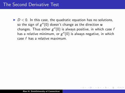
I D < 0. In this case, the quadratic equation has no solutions,so the sign of g ′′(0) doesn’t change as the direction uchanges. Thus either g ′′(0) is always positive, in which case fhas a relative minimum,
or g ′′(0) is always negative, in whichcase f has a relative maximum. We can check which case weare in by checking the sign of fxx .
I D = 0. In this case, anything can happen. This occurs forf (x , y) = x4 − y4 at the origin, where there is a saddle point,but also occurs for f (x , y) = x4 + y4 at the origin, wherethere is a relative minimum.
I D > 0. In this case, g ′′(0) > 0 for some direction vectors ubut g ′′(0) < 0 for some other direction vectors and the graphhas a saddle point.
Alan H. SteinUniversity of Connecticut
The Second Derivative Test
I D < 0. In this case, the quadratic equation has no solutions,so the sign of g ′′(0) doesn’t change as the direction uchanges. Thus either g ′′(0) is always positive, in which case fhas a relative minimum, or g ′′(0) is always negative, in whichcase f has a relative maximum.
We can check which case weare in by checking the sign of fxx .
I D = 0. In this case, anything can happen. This occurs forf (x , y) = x4 − y4 at the origin, where there is a saddle point,but also occurs for f (x , y) = x4 + y4 at the origin, wherethere is a relative minimum.
I D > 0. In this case, g ′′(0) > 0 for some direction vectors ubut g ′′(0) < 0 for some other direction vectors and the graphhas a saddle point.
Alan H. SteinUniversity of Connecticut

The Second Derivative Test
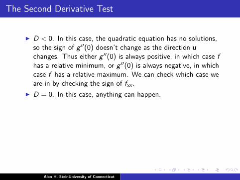
I D < 0. In this case, the quadratic equation has no solutions,so the sign of g ′′(0) doesn’t change as the direction uchanges. Thus either g ′′(0) is always positive, in which case fhas a relative minimum, or g ′′(0) is always negative, in whichcase f has a relative maximum. We can check which case weare in by checking the sign of fxx .
I D = 0. In this case, anything can happen. This occurs forf (x , y) = x4 − y4 at the origin, where there is a saddle point,but also occurs for f (x , y) = x4 + y4 at the origin, wherethere is a relative minimum.
I D > 0. In this case, g ′′(0) > 0 for some direction vectors ubut g ′′(0) < 0 for some other direction vectors and the graphhas a saddle point.
Alan H. SteinUniversity of Connecticut

The Second Derivative Test
I D < 0. In this case, the quadratic equation has no solutions,so the sign of g ′′(0) doesn’t change as the direction uchanges. Thus either g ′′(0) is always positive, in which case fhas a relative minimum, or g ′′(0) is always negative, in whichcase f has a relative maximum. We can check which case weare in by checking the sign of fxx .
I D = 0.
In this case, anything can happen. This occurs forf (x , y) = x4 − y4 at the origin, where there is a saddle point,but also occurs for f (x , y) = x4 + y4 at the origin, wherethere is a relative minimum.
I D > 0. In this case, g ′′(0) > 0 for some direction vectors ubut g ′′(0) < 0 for some other direction vectors and the graphhas a saddle point.
Alan H. SteinUniversity of Connecticut
The Second Derivative Test
I D < 0. In this case, the quadratic equation has no solutions,so the sign of g ′′(0) doesn’t change as the direction uchanges. Thus either g ′′(0) is always positive, in which case fhas a relative minimum, or g ′′(0) is always negative, in whichcase f has a relative maximum. We can check which case weare in by checking the sign of fxx .
I D = 0. In this case, anything can happen.
This occurs forf (x , y) = x4 − y4 at the origin, where there is a saddle point,but also occurs for f (x , y) = x4 + y4 at the origin, wherethere is a relative minimum.
I D > 0. In this case, g ′′(0) > 0 for some direction vectors ubut g ′′(0) < 0 for some other direction vectors and the graphhas a saddle point.
Alan H. SteinUniversity of Connecticut


The Second Derivative Test
I D < 0. In this case, the quadratic equation has no solutions,so the sign of g ′′(0) doesn’t change as the direction uchanges. Thus either g ′′(0) is always positive, in which case fhas a relative minimum, or g ′′(0) is always negative, in whichcase f has a relative maximum. We can check which case weare in by checking the sign of fxx .
I D = 0. In this case, anything can happen. This occurs forf (x , y) = x4 − y4 at the origin, where there is a saddle point,but also occurs for f (x , y) = x4 + y4 at the origin, wherethere is a relative minimum.
I D > 0. In this case, g ′′(0) > 0 for some direction vectors ubut g ′′(0) < 0 for some other direction vectors and the graphhas a saddle point.
Alan H. SteinUniversity of Connecticut

Extrema with Constraints
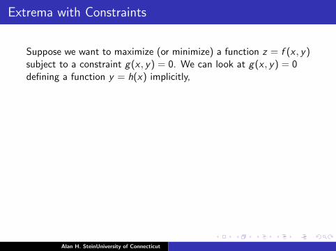
Suppose we want to maximize (or minimize) a function z = f (x , y)subject to a constraint g(x , y) = 0.
We can look at g(x , y) = 0defining a function y = h(x) implicitly, so z = f (x , h(x)).
Any extrema must occur wheredz
dx= 0.
Using the Chain Rule,dz
dx= f1(x , y)
dx
dx+ f2(x , y)
dy
dx= f1 + f2(x , y)
dy
dx.
Since y = h(x) is defined implicitly by g(x , y) = 0, we havedy
dx= −g1
g2, so
dz
dx= f1(x , y) + f2(x , y)
(−g1
g2
).
We thus must have f1(x , y)− f2(x , y)g1
g2= 0,
Alan H. SteinUniversity of Connecticut
Extrema with Constraints
Suppose we want to maximize (or minimize) a function z = f (x , y)subject to a constraint g(x , y) = 0. We can look at g(x , y) = 0defining a function y = h(x) implicitly,
so z = f (x , h(x)).
Any extrema must occur wheredz
dx= 0.
Using the Chain Rule,dz
dx= f1(x , y)
dx
dx+ f2(x , y)
dy
dx= f1 + f2(x , y)
dy
dx.
Since y = h(x) is defined implicitly by g(x , y) = 0, we havedy
dx= −g1
g2, so
dz
dx= f1(x , y) + f2(x , y)
(−g1
g2
).
We thus must have f1(x , y)− f2(x , y)g1
g2= 0,
Alan H. SteinUniversity of Connecticut

Extrema with Constraints
Suppose we want to maximize (or minimize) a function z = f (x , y)subject to a constraint g(x , y) = 0. We can look at g(x , y) = 0defining a function y = h(x) implicitly, so z = f (x , h(x)).
Any extrema must occur wheredz
dx= 0.
Using the Chain Rule,dz
dx= f1(x , y)
dx
dx+ f2(x , y)
dy
dx= f1 + f2(x , y)
dy
dx.
Since y = h(x) is defined implicitly by g(x , y) = 0,
we havedy
dx= −g1
g2, so
dz
dx= f1(x , y) + f2(x , y)
(−g1
g2
).
We thus must have f1(x , y)− f2(x , y)g1
g2= 0,
Alan H. SteinUniversity of Connecticut

Extrema with Constraints
Suppose we want to maximize (or minimize) a function z = f (x , y)subject to a constraint g(x , y) = 0. We can look at g(x , y) = 0defining a function y = h(x) implicitly, so z = f (x , h(x)).
Any extrema must occur wheredz
dx= 0.
Using the Chain Rule,dz
dx= f1(x , y)
dx
dx+ f2(x , y)
dy
dx= f1 + f2(x , y)
dy
dx.
Since y = h(x) is defined implicitly by g(x , y) = 0, we havedy
dx= −g1
g2,
sodz
dx= f1(x , y) + f2(x , y)
(−g1
g2
).
We thus must have f1(x , y)− f2(x , y)g1
g2= 0,
Alan H. SteinUniversity of Connecticut

Extrema with Constraints
Suppose we want to maximize (or minimize) a function z = f (x , y)subject to a constraint g(x , y) = 0. We can look at g(x , y) = 0defining a function y = h(x) implicitly, so z = f (x , h(x)).
Any extrema must occur wheredz
dx= 0.
Using the Chain Rule,dz
dx= f1(x , y)
dx
dx+ f2(x , y)
dy
dx= f1 + f2(x , y)
dy
dx.
Since y = h(x) is defined implicitly by g(x , y) = 0, we havedy
dx= −g1
g2, so
dz
dx= f1(x , y) + f2(x , y)
(−g1
g2
).
We thus must have f1(x , y)− f2(x , y)g1
g2= 0,
Alan H. SteinUniversity of Connecticut

Extrema with Constraints
Suppose we want to maximize (or minimize) a function z = f (x , y)subject to a constraint g(x , y) = 0. We can look at g(x , y) = 0defining a function y = h(x) implicitly, so z = f (x , h(x)).
Any extrema must occur wheredz
dx= 0.
Using the Chain Rule,dz
dx= f1(x , y)
dx
dx+ f2(x , y)
dy
dx= f1 + f2(x , y)
dy
dx.
Since y = h(x) is defined implicitly by g(x , y) = 0, we havedy
dx= −g1
g2, so
dz
dx= f1(x , y) + f2(x , y)
(−g1
g2
).
We thus must have f1(x , y)− f2(x , y)g1
g2= 0,
Alan H. SteinUniversity of Connecticut
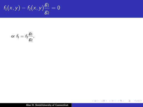
f1(x , y)− f2(x , y)g1
g2= 0
or f1 = f2g1
g2,
orf1f2
=g1
g2.
Equivalently, the vectors 5f and 5g are proportional to eachother, or 5f = λ5 g for some constant λ.This gives the method of Lagrange Multipliers: Any extrema forf (x , y) subject to the constraint g(x , y) = 0 must occur at a pointwhere 5f = λ5 g .
Alan H. SteinUniversity of Connecticut
f1(x , y)− f2(x , y)g1
g2= 0
or f1 = f2g1
g2,
orf1f2
=g1
g2.
Equivalently, the vectors 5f and 5g are proportional to eachother,
or 5f = λ5 g for some constant λ.This gives the method of Lagrange Multipliers: Any extrema forf (x , y) subject to the constraint g(x , y) = 0 must occur at a pointwhere 5f = λ5 g .
Alan H. SteinUniversity of Connecticut

f1(x , y)− f2(x , y)g1
g2= 0
or f1 = f2g1
g2,
orf1f2
=g1
g2.
Equivalently, the vectors 5f and 5g are proportional to eachother, or 5f = λ5 g for some constant λ.This gives the method of Lagrange Multipliers:
Any extrema forf (x , y) subject to the constraint g(x , y) = 0 must occur at a pointwhere 5f = λ5 g .
Alan H. SteinUniversity of Connecticut
f1(x , y)− f2(x , y)g1
g2= 0
or f1 = f2g1
g2,
orf1f2
=g1
g2.
Equivalently, the vectors 5f and 5g are proportional to eachother, or 5f = λ5 g for some constant λ.This gives the method of Lagrange Multipliers: Any extrema forf (x , y) subject to the constraint g(x , y) = 0 must occur at a pointwhere 5f = λ5 g .
Alan H. SteinUniversity of Connecticut

Lagrange Multipliers
In practice, this means we simultaneously solve the system ofequations:
∂f
∂x= λ
∂g
∂x∂f
∂y= λ
∂g
∂y
g(x , y) = 0.
Alan H. SteinUniversity of Connecticut

A Geometric Perspective
Any maximum M for a function f (x , y) subject to a constraintg(x , y) = 0 occurs at a point where the graphs of f (x , y) = M andg(x , y) = 0 meet.
One would expect that f (x , y) > M on one sideof the graph of f (x , y) = M and f (x , y) < M on the other side.
It would thus appear the graphs of f (x , y) = M and g(x , y) = 0are tangent, since otherwise there would be points on g(x , y) = 0on either side of the graph of f (x , y) = M, and M wouldn’t be amaximum.
A similar argument could be made for a minimum.
Thus, the tangent lines to f (x , y) = M and g(x , y) = 0 at theextremum coincide, and must have parallel normals.
Since 5f is normal to the tangent to f (x , y) = M and 5g isnormal to the tangent to g(x , y) = 0, so it follows 5f = λ5 g forsome scalar λ.
Alan H. SteinUniversity of Connecticut

A Geometric Perspective
Any maximum M for a function f (x , y) subject to a constraintg(x , y) = 0 occurs at a point where the graphs of f (x , y) = M andg(x , y) = 0 meet. One would expect that f (x , y) > M on one sideof the graph of f (x , y) = M and f (x , y) < M on the other side.
It would thus appear the graphs of f (x , y) = M and g(x , y) = 0are tangent, since otherwise there would be points on g(x , y) = 0on either side of the graph of f (x , y) = M, and M wouldn’t be amaximum.
A similar argument could be made for a minimum.
Thus, the tangent lines to f (x , y) = M and g(x , y) = 0 at theextremum coincide, and must have parallel normals.
Since 5f is normal to the tangent to f (x , y) = M and 5g isnormal to the tangent to g(x , y) = 0, so it follows 5f = λ5 g forsome scalar λ.
Alan H. SteinUniversity of Connecticut
A Geometric Perspective
Any maximum M for a function f (x , y) subject to a constraintg(x , y) = 0 occurs at a point where the graphs of f (x , y) = M andg(x , y) = 0 meet. One would expect that f (x , y) > M on one sideof the graph of f (x , y) = M and f (x , y) < M on the other side.
It would thus appear the graphs of f (x , y) = M and g(x , y) = 0are tangent, since otherwise there would be points on g(x , y) = 0on either side of the graph of f (x , y) = M,
and M wouldn’t be amaximum.
A similar argument could be made for a minimum.
Thus, the tangent lines to f (x , y) = M and g(x , y) = 0 at theextremum coincide, and must have parallel normals.
Since 5f is normal to the tangent to f (x , y) = M and 5g isnormal to the tangent to g(x , y) = 0, so it follows 5f = λ5 g forsome scalar λ.
Alan H. SteinUniversity of Connecticut

A Geometric Perspective
Any maximum M for a function f (x , y) subject to a constraintg(x , y) = 0 occurs at a point where the graphs of f (x , y) = M andg(x , y) = 0 meet. One would expect that f (x , y) > M on one sideof the graph of f (x , y) = M and f (x , y) < M on the other side.
It would thus appear the graphs of f (x , y) = M and g(x , y) = 0are tangent, since otherwise there would be points on g(x , y) = 0on either side of the graph of f (x , y) = M, and M wouldn’t be amaximum.
A similar argument could be made for a minimum.
Thus, the tangent lines to f (x , y) = M and g(x , y) = 0 at theextremum coincide, and must have parallel normals.
Since 5f is normal to the tangent to f (x , y) = M and 5g isnormal to the tangent to g(x , y) = 0, so it follows 5f = λ5 g forsome scalar λ.
Alan H. SteinUniversity of Connecticut
A Geometric Perspective
Any maximum M for a function f (x , y) subject to a constraintg(x , y) = 0 occurs at a point where the graphs of f (x , y) = M andg(x , y) = 0 meet. One would expect that f (x , y) > M on one sideof the graph of f (x , y) = M and f (x , y) < M on the other side.
It would thus appear the graphs of f (x , y) = M and g(x , y) = 0are tangent, since otherwise there would be points on g(x , y) = 0on either side of the graph of f (x , y) = M, and M wouldn’t be amaximum.
A similar argument could be made for a minimum.
Thus, the tangent lines to f (x , y) = M and g(x , y) = 0 at theextremum coincide,
and must have parallel normals.
Since 5f is normal to the tangent to f (x , y) = M and 5g isnormal to the tangent to g(x , y) = 0, so it follows 5f = λ5 g forsome scalar λ.
Alan H. SteinUniversity of Connecticut

A Geometric Perspective
Any maximum M for a function f (x , y) subject to a constraintg(x , y) = 0 occurs at a point where the graphs of f (x , y) = M andg(x , y) = 0 meet. One would expect that f (x , y) > M on one sideof the graph of f (x , y) = M and f (x , y) < M on the other side.
It would thus appear the graphs of f (x , y) = M and g(x , y) = 0are tangent, since otherwise there would be points on g(x , y) = 0on either side of the graph of f (x , y) = M, and M wouldn’t be amaximum.
A similar argument could be made for a minimum.
Thus, the tangent lines to f (x , y) = M and g(x , y) = 0 at theextremum coincide, and must have parallel normals.
Since 5f is normal to the tangent to f (x , y) = M and 5g isnormal to the tangent to g(x , y) = 0, so it follows 5f = λ5 g forsome scalar λ.
Alan H. SteinUniversity of Connecticut

A Geometric Perspective
Any maximum M for a function f (x , y) subject to a constraintg(x , y) = 0 occurs at a point where the graphs of f (x , y) = M andg(x , y) = 0 meet. One would expect that f (x , y) > M on one sideof the graph of f (x , y) = M and f (x , y) < M on the other side.
It would thus appear the graphs of f (x , y) = M and g(x , y) = 0are tangent, since otherwise there would be points on g(x , y) = 0on either side of the graph of f (x , y) = M, and M wouldn’t be amaximum.
A similar argument could be made for a minimum.
Thus, the tangent lines to f (x , y) = M and g(x , y) = 0 at theextremum coincide, and must have parallel normals.
Since 5f is normal to the tangent to f (x , y) = M
and 5g isnormal to the tangent to g(x , y) = 0, so it follows 5f = λ5 g forsome scalar λ.
Alan H. SteinUniversity of Connecticut

A Geometric Perspective
Any maximum M for a function f (x , y) subject to a constraintg(x , y) = 0 occurs at a point where the graphs of f (x , y) = M andg(x , y) = 0 meet. One would expect that f (x , y) > M on one sideof the graph of f (x , y) = M and f (x , y) < M on the other side.
It would thus appear the graphs of f (x , y) = M and g(x , y) = 0are tangent, since otherwise there would be points on g(x , y) = 0on either side of the graph of f (x , y) = M, and M wouldn’t be amaximum.
A similar argument could be made for a minimum.
Thus, the tangent lines to f (x , y) = M and g(x , y) = 0 at theextremum coincide, and must have parallel normals.
Since 5f is normal to the tangent to f (x , y) = M and 5g isnormal to the tangent to g(x , y) = 0,
so it follows 5f = λ5 g forsome scalar λ.
Alan H. SteinUniversity of Connecticut
A Geometric Perspective
Any maximum M for a function f (x , y) subject to a constraintg(x , y) = 0 occurs at a point where the graphs of f (x , y) = M andg(x , y) = 0 meet. One would expect that f (x , y) > M on one sideof the graph of f (x , y) = M and f (x , y) < M on the other side.
It would thus appear the graphs of f (x , y) = M and g(x , y) = 0are tangent, since otherwise there would be points on g(x , y) = 0on either side of the graph of f (x , y) = M, and M wouldn’t be amaximum.
A similar argument could be made for a minimum.
Thus, the tangent lines to f (x , y) = M and g(x , y) = 0 at theextremum coincide, and must have parallel normals.
Since 5f is normal to the tangent to f (x , y) = M and 5g isnormal to the tangent to g(x , y) = 0, so it follows 5f = λ5 g forsome scalar λ.
Alan H. SteinUniversity of Connecticut
Multiple Constraints and Higher Dimensions
If there are multiple constraints, the gradient of the function to beoptimized must be a linear combination of the gradients of thefunctions defining the constraints.
In higher dimensions, the obvious analogue holds.
Alan H. SteinUniversity of Connecticut
Multiple Constraints and Higher Dimensions
If there are multiple constraints, the gradient of the function to beoptimized must be a linear combination of the gradients of thefunctions defining the constraints.
In higher dimensions, the obvious analogue holds.
Alan H. SteinUniversity of Connecticut
![Extremum Seeking Control: Convergence Analysis · extremum seeking as one of the most promising adaptive control methods [1, Section 13.3]. There are two main approaches to extremum](https://img.pdfslide.us/doc/110x75/5e1ecc5cc0fc09187723051d/extremum-seeking-control-convergence-analysis-extremum-seeking-as-one-of-the-most.jpg)