Embed Size (px)
Citation preview
Functions of Several Variables
A function of several variables is just what it sounds like.
It may beviewed in at least three different ways. We will use a function oftwo variables as an example.
I z = f (x , y) may be viewed as a function of the twoindependent variables x , y .
I It may be viewed as a function defined at different points(x , y) in the plane.
I It may be viewed as a function whose domain is the set ofvectors < x , y > or x i + y j.
Alan H. SteinUniversity of Connecticut
Functions of Several Variables
A function of several variables is just what it sounds like. It may beviewed in at least three different ways. We will use a function oftwo variables as an example.
I z = f (x , y) may be viewed as a function of the twoindependent variables x , y .
I It may be viewed as a function defined at different points(x , y) in the plane.
I It may be viewed as a function whose domain is the set ofvectors < x , y > or x i + y j.
Alan H. SteinUniversity of Connecticut
Limits of Functions of Several Variables
We define a limit of a function of several variables essentially thesame way we define a limit for an ordinary function:
Definition (Limit)
limx→c f (x) = L if ∀ε > 0, ∃δ > 0 such that |f (x)− L| < εwhenever 0 < |x − c | < δ.
Definition (Limit)
limx→c f (x) = L if ∀ε > 0, ∃δ > 0 such that |f (x)− L| < εwhenever 0 < |x− c| < δ.
Alan H. SteinUniversity of Connecticut
Properties of Limits
Rule of Thumb: If a property of limits makes sense whentranslated to refer to a limit of a function of several variables, thenit is valid for a function of several variables.
For example, the limit of a sum will be the sum of the limits, thelimit of a difference will be the difference of the limits, the limit ofa product will be the product of the limits and the limit of aquotient will be the quotient of the limits, provided the latter limitexists.
Alan H. SteinUniversity of Connecticut
Properties of Limits
Rule of Thumb: If a property of limits makes sense whentranslated to refer to a limit of a function of several variables, thenit is valid for a function of several variables.
For example, the limit of a sum will be the sum of the limits,
thelimit of a difference will be the difference of the limits, the limit ofa product will be the product of the limits and the limit of aquotient will be the quotient of the limits, provided the latter limitexists.
Alan H. SteinUniversity of Connecticut

Properties of Limits
Rule of Thumb: If a property of limits makes sense whentranslated to refer to a limit of a function of several variables, thenit is valid for a function of several variables.
For example, the limit of a sum will be the sum of the limits, thelimit of a difference will be the difference of the limits,
the limit ofa product will be the product of the limits and the limit of aquotient will be the quotient of the limits, provided the latter limitexists.
Alan H. SteinUniversity of Connecticut
Properties of Limits
Rule of Thumb: If a property of limits makes sense whentranslated to refer to a limit of a function of several variables, thenit is valid for a function of several variables.
For example, the limit of a sum will be the sum of the limits, thelimit of a difference will be the difference of the limits, the limit ofa product will be the product of the limits
and the limit of aquotient will be the quotient of the limits, provided the latter limitexists.
Alan H. SteinUniversity of Connecticut

Properties of Limits
Rule of Thumb: If a property of limits makes sense whentranslated to refer to a limit of a function of several variables, thenit is valid for a function of several variables.
For example, the limit of a sum will be the sum of the limits, thelimit of a difference will be the difference of the limits, the limit ofa product will be the product of the limits and the limit of aquotient will be the quotient of the limits, provided the latter limitexists.
Alan H. SteinUniversity of Connecticut
Continuity
The definition of continuity for a function of several variables isessentially the same as the definition for an ordinary function.
Definition (Continuity)
A function f is continuous at c iflimx→c f (x) = f (c).
Definition (Continuity for a Function of Several Variables)
A function f is continuous at c if limx→c f (x) = f (c).
As with ordinary functions, functions of several variables willgenerally be continuous except where there’s an obvious reason forthem not to be.
Alan H. SteinUniversity of Connecticut
Partial Derivatives
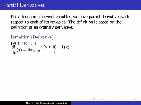
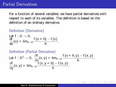
For a function of several variables, we have partial derivatives withrespect to each of its variables. The definition is based on thedefinition of an ordinary derivative.
Definition (Derivative)
Let f : R → R.df
dx(x) = limh→0
f (x + h)− f (x)
h.
Definition (Partial Derivative)
Let f : R2 → R.∂f
∂x(x , y) = limh→0
f (x + h, y)− f (x , y)
h,
∂f
∂y(x , y) = limh→0
f (x , y + h)− f (x , y)
h.
The obvious generalizations hold for functions with more than twoindependent variables.
Alan H. SteinUniversity of Connecticut
Partial Derivatives
For a function of several variables, we have partial derivatives withrespect to each of its variables. The definition is based on thedefinition of an ordinary derivative.
Definition (Derivative)
Let f : R → R.df
dx(x) = limh→0
f (x + h)− f (x)
h.
Definition (Partial Derivative)
Let f : R2 → R.∂f
∂x(x , y) = limh→0
f (x + h, y)− f (x , y)
h,
∂f
∂y(x , y) = limh→0
f (x , y + h)− f (x , y)
h.
The obvious generalizations hold for functions with more than twoindependent variables.
Alan H. SteinUniversity of Connecticut

Calculation of Partial Derivatives
Effectively, we calculate the partial derivative of a function withrespect to one of its independent variables by acting as if the otherindependent variables were actually constants.
Alan H. SteinUniversity of Connecticut
Notation
The following notations for the partial derivatives of a functionz = f (x , y) are equivalent.
fx =∂f
∂x=
∂z
∂x= f1 = D1f = Dx f
fy =∂f
∂y=
∂z
∂y= f2 = D2f = Dy f
Alan H. SteinUniversity of Connecticut

Notation
The following notations for the partial derivatives of a functionz = f (x , y) are equivalent.
fx =∂f
∂x=
∂z
∂x= f1 = D1f = Dx f
fy =∂f
∂y=
∂z
∂y= f2 = D2f = Dy f
Alan H. SteinUniversity of Connecticut

Notation
The following notations for the partial derivatives of a functionz = f (x , y) are equivalent.
fx =∂f
∂x=
∂z
∂x= f1 = D1f = Dx f
fy =∂f
∂y=
∂z
∂y= f2 = D2f = Dy f
Alan H. SteinUniversity of Connecticut
Higher Order Derivatives
Since a partial derivative is itself a function of several variables, ithas its own partial derivatives.
(fx)y = fxy = f12 =∂
∂y
(∂f
∂x
)=
∂2f
∂y∂x=
∂2z
∂y∂x
(fy )x = fyx = f21 =∂
∂x
(∂f
∂y
)=
∂2f
∂x∂y=
∂2z
∂x∂y
Alan H. SteinUniversity of Connecticut

Higher Order Derivatives
Since a partial derivative is itself a function of several variables, ithas its own partial derivatives.
(fx)y = fxy = f12 =∂
∂y
(∂f
∂x
)=
∂2f
∂y∂x=
∂2z
∂y∂x
(fy )x = fyx = f21 =∂
∂x
(∂f
∂y
)=
∂2f
∂x∂y=
∂2z
∂x∂y
Alan H. SteinUniversity of Connecticut

Higher Order Derivatives
Since a partial derivative is itself a function of several variables, ithas its own partial derivatives.
(fx)y = fxy = f12 =∂
∂y
(∂f
∂x
)=
∂2f
∂y∂x=
∂2z
∂y∂x
(fy )x = fyx = f21 =∂
∂x
(∂f
∂y
)=
∂2f
∂x∂y=
∂2z
∂x∂y
Alan H. SteinUniversity of Connecticut
Changing the Order of Differentiation
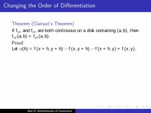
Theorem (Clairaut’s Theorem)
If fxy and fyx are both continuous on a disk containing (a, b), thenfxy (a, b) = fyx(a, b).
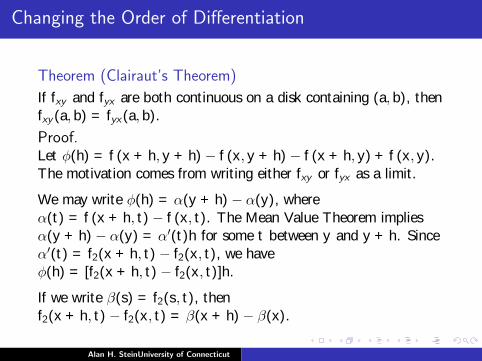
Proof.Let φ(h) = f (x + h, y + h)− f (x , y + h)− f (x + h, y) + f (x , y).
The motivation comes from writing either fxy or fyx as a limit.
We may write φ(h) = α(y + h)− α(y), whereα(t) = f (x + h, t)− f (x , t). The Mean Value Theorem impliesα(y + h)− α(y) = α′(t)h for some t between y and y + h. Sinceα′(t) = f2(x + h, t)− f2(x , t), we haveφ(h) = [f2(x + h, t)− f2(x , t)]h.
If we write β(s) = f2(s, t), thenf2(x + h, t)− f2(x , t) = β(x + h)− β(x).
Alan H. SteinUniversity of Connecticut
Changing the Order of Differentiation
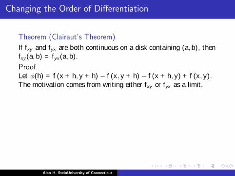
Theorem (Clairaut’s Theorem)
If fxy and fyx are both continuous on a disk containing (a, b), thenfxy (a, b) = fyx(a, b).
Proof.Let φ(h) = f (x + h, y + h)− f (x , y + h)− f (x + h, y) + f (x , y).The motivation comes from writing either fxy or fyx as a limit.
We may write φ(h) = α(y + h)− α(y), whereα(t) = f (x + h, t)− f (x , t). The Mean Value Theorem impliesα(y + h)− α(y) = α′(t)h for some t between y and y + h. Sinceα′(t) = f2(x + h, t)− f2(x , t), we haveφ(h) = [f2(x + h, t)− f2(x , t)]h.
If we write β(s) = f2(s, t), thenf2(x + h, t)− f2(x , t) = β(x + h)− β(x).
Alan H. SteinUniversity of Connecticut
Changing the Order of Differentiation
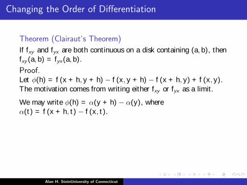
Theorem (Clairaut’s Theorem)
If fxy and fyx are both continuous on a disk containing (a, b), thenfxy (a, b) = fyx(a, b).
Proof.Let φ(h) = f (x + h, y + h)− f (x , y + h)− f (x + h, y) + f (x , y).The motivation comes from writing either fxy or fyx as a limit.
We may write φ(h) = α(y + h)− α(y), whereα(t) = f (x + h, t)− f (x , t).
The Mean Value Theorem impliesα(y + h)− α(y) = α′(t)h for some t between y and y + h. Sinceα′(t) = f2(x + h, t)− f2(x , t), we haveφ(h) = [f2(x + h, t)− f2(x , t)]h.
If we write β(s) = f2(s, t), thenf2(x + h, t)− f2(x , t) = β(x + h)− β(x).
Alan H. SteinUniversity of Connecticut

Changing the Order of Differentiation
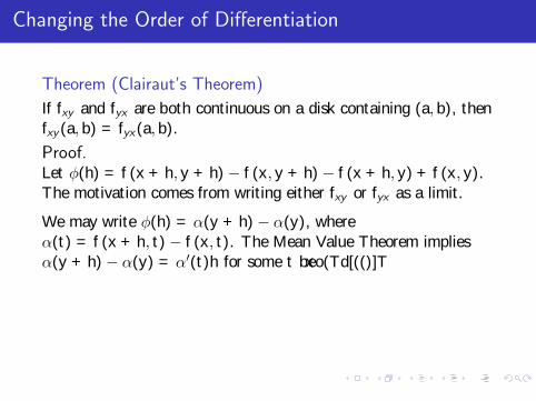
Theorem (Clairaut’s Theorem)
If fxy and fyx are both continuous on a disk containing (a, b), thenfxy (a, b) = fyx(a, b).
Proof.Let φ(h) = f (x + h, y + h)− f (x , y + h)− f (x + h, y) + f (x , y).The motivation comes from writing either fxy or fyx as a limit.
We may write φ(h) = α(y + h)− α(y), whereα(t) = f (x + h, t)− f (x , t). The Mean Value Theorem impliesα(y + h)− α(y) = α′(t)h for some t between y and y + h. Sinceα′(t) = f2(x + h, t)− f2(x , t), we haveφ(h) = [f2(x + h, t)− f2(x , t)]h.
If we write β(s) = f2(s, t), thenf2(x + h, t)− f2(x , t) = β(x + h)− β(x).
Alan H. SteinUniversity of Connecticut
Changing the Order of Differentiation
Theorem (Clairaut’s Theorem)
If fxy and fyx are both continuous on a disk containing (a, b), thenfxy (a, b) = fyx(a, b).
Proof.Let φ(h) = f (x + h, y + h)− f (x , y + h)− f (x + h, y) + f (x , y).The motivation comes from writing either fxy or fyx as a limit.
We may write φ(h) = α(y + h)− α(y), whereα(t) = f (x + h, t)− f (x , t). The Mean Value Theorem impliesα(y + h)− α(y) = α′(t)h for some t between y and y + h. Sinceα′(t) = f2(x + h, t)− f2(x , t), we haveφ(h) = [f2(x + h, t)− f2(x , t)]h.
If we write β(s) = f2(s, t), thenf2(x + h, t)− f2(x , t) = β(x + h)− β(x).
Alan H. SteinUniversity of Connecticut

Clairault’s Theorem
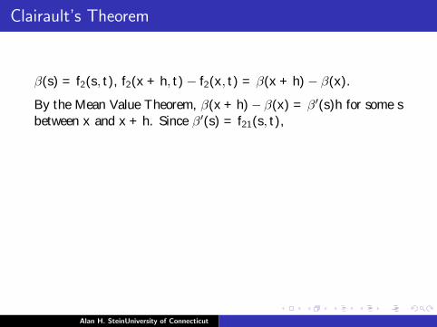
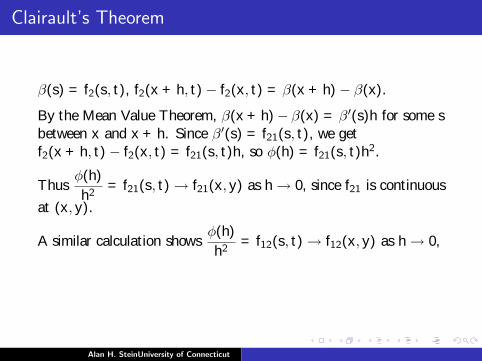
β(s) = f2(s, t), f2(x + h, t)− f2(x , t) = β(x + h)− β(x).
By the Mean Value Theorem, β(x + h)− β(x) = β′(s)h for some sbetween x and x + h. Since β′(s) = f21(s, t), we getf2(x + h, t)− f2(x , t) = f21(s, t)h, so φ(h) = f21(s, t)h2.
Thusφ(h)
h2= f21(s, t) → f21(x , y) as h → 0, since f21 is continuous
at (x , y).
A similar calculation showsφ(h)
h2= f12(s, t) → f12(x , y) as h → 0,
showing f12(x , y) = f21(x , y).
Alan H. SteinUniversity of Connecticut

Clairault’s Theorem
β(s) = f2(s, t), f2(x + h, t)− f2(x , t) = β(x + h)− β(x).
By the Mean Value Theorem, β(x + h)− β(x) = β′(s)h for some sbetween x and x + h.
Since β′(s) = f21(s, t), we getf2(x + h, t)− f2(x , t) = f21(s, t)h, so φ(h) = f21(s, t)h2.
Thusφ(h)
h2= f21(s, t) → f21(x , y) as h → 0, since f21 is continuous
at (x , y).
A similar calculation showsφ(h)
h2= f12(s, t) → f12(x , y) as h → 0,
showing f12(x , y) = f21(x , y).
Alan H. SteinUniversity of Connecticut
Clairault’s Theorem
β(s) = f2(s, t), f2(x + h, t)− f2(x , t) = β(x + h)− β(x).
By the Mean Value Theorem, β(x + h)− β(x) = β′(s)h for some sbetween x and x + h. Since β′(s) = f21(s, t),
we getf2(x + h, t)− f2(x , t) = f21(s, t)h, so φ(h) = f21(s, t)h2.
Thusφ(h)
h2= f21(s, t) → f21(x , y) as h → 0, since f21 is continuous
at (x , y).
A similar calculation showsφ(h)
h2= f12(s, t) → f12(x , y) as h → 0,
showing f12(x , y) = f21(x , y).
Alan H. SteinUniversity of Connecticut

Clairault’s Theorem
β(s) = f2(s, t), f2(x + h, t)− f2(x , t) = β(x + h)− β(x).
By the Mean Value Theorem, β(x + h)− β(x) = β′(s)h for some sbetween x and x + h. Since β′(s) = f21(s, t), we getf2(x + h, t)− f2(x , t) = f21(s, t)h, so
φ(h) = f21(s, t)h2.
Thusφ(h)
h2= f21(s, t) → f21(x , y) as h → 0, since f21 is continuous
at (x , y).
A similar calculation showsφ(h)
h2= f12(s, t) → f12(x , y) as h → 0,
showing f12(x , y) = f21(x , y).
Alan H. SteinUniversity of Connecticut

Clairault’s Theorem
β(s) = f2(s, t), f2(x + h, t)− f2(x , t) = β(x + h)− β(x).
By the Mean Value Theorem, β(x + h)− β(x) = β′(s)h for some sbetween x and x + h. Since β′(s) = f21(s, t), we getf2(x + h, t)− f2(x , t) = f21(s, t)h, so φ(h) = f21(s, t)h2.
Thusφ(h)
h2= f21(s, t) → f21(x , y) as h → 0, since f21 is continuous
at (x , y).
A similar calculation showsφ(h)
h2= f12(s, t) → f12(x , y) as h → 0,
showing f12(x , y) = f21(x , y).
Alan H. SteinUniversity of Connecticut

Clairault’s Theorem
β(s) = f2(s, t), f2(x + h, t)− f2(x , t) = β(x + h)− β(x).
By the Mean Value Theorem, β(x + h)− β(x) = β′(s)h for some sbetween x and x + h. Since β′(s) = f21(s, t), we getf2(x + h, t)− f2(x , t) = f21(s, t)h, so φ(h) = f21(s, t)h2.
Thusφ(h)
h2= f21(s, t) → f21(x , y) as h → 0, since f21 is continuous
at (x , y).
A similar calculation showsφ(h)
h2= f12(s, t) → f12(x , y) as h → 0,
showing f12(x , y) = f21(x , y).
Alan H. SteinUniversity of Connecticut

Tangent Planes
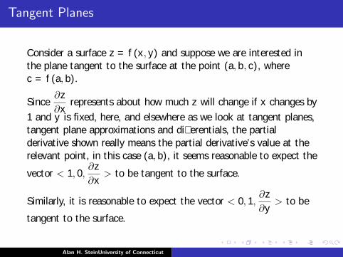
Consider a surface z = f (x , y) and suppose we are interested inthe plane tangent to the surface at the point (a, b, c), wherec = f (a, b).
Since∂z
∂xrepresents about how much z will change if x changes by
1 and y is fixed, here, and elsewhere as we look at tangent planes,tangent plane approximations and differentials, the partialderivative shown really means the partial derivative’s value at therelevant point, in this case (a, b), it seems reasonable to expect the
vector < 1, 0,∂z
∂x> to be tangent to the surface.
Similarly, it is reasonable to expect the vector < 0, 1,∂z
∂y> to be
tangent to the surface.
Alan H. SteinUniversity of Connecticut

Tangent Planes
Consider a surface z = f (x , y) and suppose we are interested inthe plane tangent to the surface at the point (a, b, c), wherec = f (a, b).
Since∂z
∂xrepresents about how much z will change if x changes by
1 and y is fixed,
here, and elsewhere as we look at tangent planes,tangent plane approximations and differentials, the partialderivative shown really means the partial derivative’s value at therelevant point, in this case (a, b), it seems reasonable to expect the
vector < 1, 0,∂z
∂x> to be tangent to the surface.
Similarly, it is reasonable to expect the vector < 0, 1,∂z
∂y> to be
tangent to the surface.
Alan H. SteinUniversity of Connecticut

Tangent Planes
Consider a surface z = f (x , y) and suppose we are interested inthe plane tangent to the surface at the point (a, b, c), wherec = f (a, b).
Since∂z
∂xrepresents about how much z will change if x changes by
1 and y is fixed, here, and elsewhere as we look at tangent planes,tangent plane approximations and differentials, the partialderivative shown really means the partial derivative’s value at therelevant point, in this case (a, b),
it seems reasonable to expect the
vector < 1, 0,∂z
∂x> to be tangent to the surface.
Similarly, it is reasonable to expect the vector < 0, 1,∂z
∂y> to be
tangent to the surface.
Alan H. SteinUniversity of Connecticut

Tangent Planes
Consider a surface z = f (x , y) and suppose we are interested inthe plane tangent to the surface at the point (a, b, c), wherec = f (a, b).
Since∂z
∂xrepresents about how much z will change if x changes by
1 and y is fixed, here, and elsewhere as we look at tangent planes,tangent plane approximations and differentials, the partialderivative shown really means the partial derivative’s value at therelevant point, in this case (a, b), it seems reasonable to expect the
vector < 1, 0,∂z
∂x> to be tangent to the surface.
Similarly, it is reasonable to expect the vector < 0, 1,∂z
∂y> to be
tangent to the surface.
Alan H. SteinUniversity of Connecticut
Tangent Planes
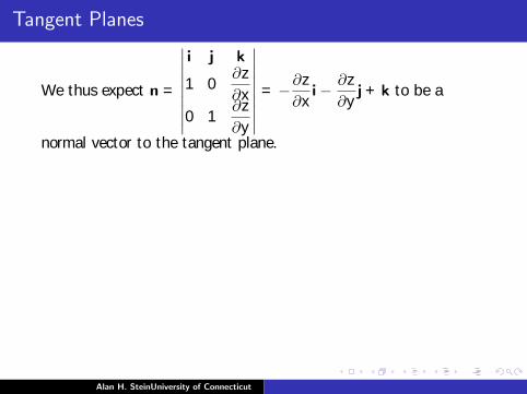
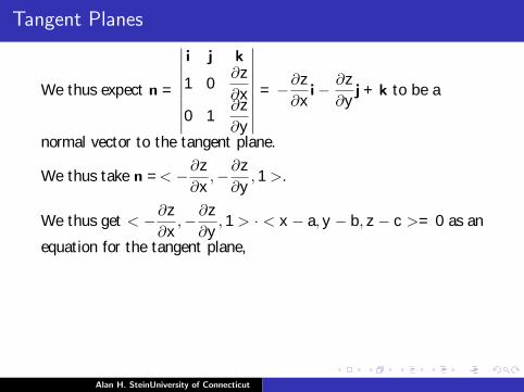
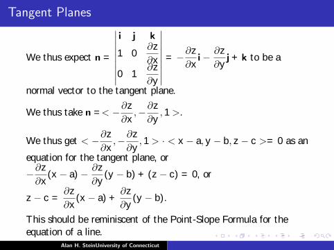
We thus expect n =
∣∣∣∣∣∣∣∣∣i j k
1 0∂z
∂x
0 1∂z
∂y
∣∣∣∣∣∣∣∣∣ = −∂z
∂xi− ∂z
∂yj + k to be a
normal vector to the tangent plane.
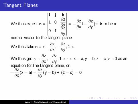
We thus take n =< −∂z
∂x,−∂z
∂y, 1 >.
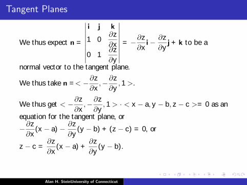
We thus get < −∂z
∂x,−∂z
∂y, 1 > · < x − a, y − b, z − c >= 0 as an
equation for the tangent plane, or
−∂z
∂x(x − a)− ∂z
∂y(y − b) + (z − c) = 0, or
z − c =∂z
∂x(x − a) +
∂z
∂y(y − b).
This should be reminiscent of the Point-Slope Formula for theequation of a line.
Alan H. SteinUniversity of Connecticut

Tangent Planes
We thus expect n =
∣∣∣∣∣∣∣∣∣i j k
1 0∂z
∂x
0 1∂z
∂y
∣∣∣∣∣∣∣∣∣ = −∂z
∂xi− ∂z
∂yj + k to be a
normal vector to the tangent plane.
We thus take n =< −∂z
∂x,−∂z
∂y, 1 >.
We thus get < −∂z
∂x,−∂z
∂y, 1 > · < x − a, y − b, z − c >= 0 as an
equation for the tangent plane, or
−∂z
∂x(x − a)− ∂z
∂y(y − b) + (z − c) = 0, or
z − c =∂z
∂x(x − a) +
∂z
∂y(y − b).
This should be reminiscent of the Point-Slope Formula for theequation of a line.
Alan H. SteinUniversity of Connecticut
Tangent Planes
We thus expect n =
∣∣∣∣∣∣∣∣∣i j k
1 0∂z
∂x
0 1∂z
∂y
∣∣∣∣∣∣∣∣∣ = −∂z
∂xi− ∂z
∂yj + k to be a
normal vector to the tangent plane.
We thus take n =< −∂z
∂x,−∂z
∂y, 1 >.
We thus get < −∂z
∂x,−∂z
∂y, 1 > · < x − a, y − b, z − c >= 0 as an
equation for the tangent plane,
or
−∂z
∂x(x − a)− ∂z
∂y(y − b) + (z − c) = 0, or
z − c =∂z
∂x(x − a) +
∂z
∂y(y − b).
This should be reminiscent of the Point-Slope Formula for theequation of a line.
Alan H. SteinUniversity of Connecticut
Tangent Planes
We thus expect n =
∣∣∣∣∣∣∣∣∣i j k
1 0∂z
∂x
0 1∂z
∂y
∣∣∣∣∣∣∣∣∣ = −∂z
∂xi− ∂z
∂yj + k to be a
normal vector to the tangent plane.
We thus take n =< −∂z
∂x,−∂z
∂y, 1 >.
We thus get < −∂z
∂x,−∂z
∂y, 1 > · < x − a, y − b, z − c >= 0 as an
equation for the tangent plane, or
−∂z
∂x(x − a)− ∂z
∂y(y − b) + (z − c) = 0,
or
z − c =∂z
∂x(x − a) +
∂z
∂y(y − b).
This should be reminiscent of the Point-Slope Formula for theequation of a line.
Alan H. SteinUniversity of Connecticut
Tangent Planes
We thus expect n =
∣∣∣∣∣∣∣∣∣i j k
1 0∂z
∂x
0 1∂z
∂y
∣∣∣∣∣∣∣∣∣ = −∂z
∂xi− ∂z
∂yj + k to be a
normal vector to the tangent plane.
We thus take n =< −∂z
∂x,−∂z
∂y, 1 >.
We thus get < −∂z
∂x,−∂z
∂y, 1 > · < x − a, y − b, z − c >= 0 as an
equation for the tangent plane, or
−∂z
∂x(x − a)− ∂z
∂y(y − b) + (z − c) = 0, or
z − c =∂z
∂x(x − a) +
∂z
∂y(y − b).
This should be reminiscent of the Point-Slope Formula for theequation of a line.
Alan H. SteinUniversity of Connecticut
Tangent Planes
We thus expect n =
∣∣∣∣∣∣∣∣∣i j k
1 0∂z
∂x
0 1∂z
∂y
∣∣∣∣∣∣∣∣∣ = −∂z
∂xi− ∂z
∂yj + k to be a
normal vector to the tangent plane.
We thus take n =< −∂z
∂x,−∂z
∂y, 1 >.
We thus get < −∂z
∂x,−∂z
∂y, 1 > · < x − a, y − b, z − c >= 0 as an
equation for the tangent plane, or
−∂z
∂x(x − a)− ∂z
∂y(y − b) + (z − c) = 0, or
z − c =∂z
∂x(x − a) +
∂z
∂y(y − b).
This should be reminiscent of the Point-Slope Formula for theequation of a line.
Alan H. SteinUniversity of Connecticut

Tangent Hyperplanes
It generalizes to
y − b =∑n
i=1
∂y
∂xi(xi − ai )
as an equation for the hyperplane tangent to the hypersurfacey = f (x1, x2, . . . , xn) at the point (a1, a2, . . . , an, b).
Alan H. SteinUniversity of Connecticut
Tangent Plane Approximations and Differentials
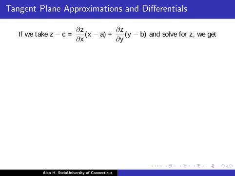
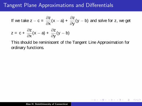
If we take z − c =∂z
∂x(x − a) +
∂z
∂y(y − b) and solve for z , we get
z = c +∂z
∂x(x − a) +
∂z
∂y(y − b)
This should be reminiscent of the Tangent Line Approximation forordinary functions.
We may use this formula to approximate f (x , y) at a point (x , y)close to a point (a, b).
Definition (Differentials)
dx = ∆x = x − ady = ∆y = y − b
dz =∂z
∂x(x − a) +
∂z
∂y(y − b)
Alan H. SteinUniversity of Connecticut

Tangent Plane Approximations and Differentials
If we take z − c =∂z
∂x(x − a) +
∂z
∂y(y − b) and solve for z , we get
z = c +∂z
∂x(x − a) +
∂z
∂y(y − b)
This should be reminiscent of the Tangent Line Approximation forordinary functions.
We may use this formula to approximate f (x , y) at a point (x , y)close to a point (a, b).
Definition (Differentials)
dx = ∆x = x − ady = ∆y = y − b
dz =∂z
∂x(x − a) +
∂z
∂y(y − b)
Alan H. SteinUniversity of Connecticut

Differentials
We may use the differential dz to approximate the change∆z = ∆f of a function f (x , y) if the independent variables x andy change by amounts dx and dy .
This generalizes in the obvious way to functions of more than twovariables.
Alan H. SteinUniversity of Connecticut
Differentials
We may use the differential dz to approximate the change∆z = ∆f of a function f (x , y) if the independent variables x andy change by amounts dx and dy .
This generalizes in the obvious way to functions of more than twovariables.
Alan H. SteinUniversity of Connecticut

Differentiability
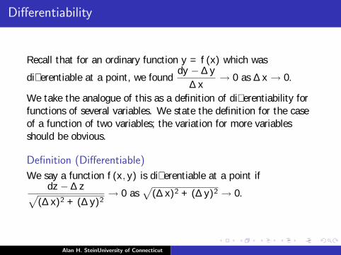
Recall that for an ordinary function y = f (x) which was
differentiable at a point, we founddy −∆y
∆x→ 0 as ∆x → 0.
We take the analogue of this as a definition of differentiability forfunctions of several variables. We state the definition for the caseof a function of two variables; the variation for more variablesshould be obvious.
Definition (Differentiable)
We say a function f (x , y) is differentiable at a point ifdz −∆z√
(∆x)2 + (∆y)2→ 0 as
√(∆x)2 + (∆y)2 → 0.
Alan H. SteinUniversity of Connecticut

Differentiability
Recall that for an ordinary function y = f (x) which was
differentiable at a point, we founddy −∆y
∆x→ 0 as ∆x → 0.
We take the analogue of this as a definition of differentiability forfunctions of several variables. We state the definition for the caseof a function of two variables; the variation for more variablesshould be obvious.
Definition (Differentiable)
We say a function f (x , y) is differentiable at a point ifdz −∆z√
(∆x)2 + (∆y)2→ 0 as
√(∆x)2 + (∆y)2 → 0.
Alan H. SteinUniversity of Connecticut
Differentiability
Recall√
(∆x)2 + (∆y)2 is the distance between (x , y) and thepoint in question.
Effectively, we are defining a function of several variables to bedifferentialbe when an approximation using differentials isreasonable.
We still need a reasonable way of determining whether a functionis differentiable. This is given by the following theorem.
Alan H. SteinUniversity of Connecticut

Differentiability
Recall√
(∆x)2 + (∆y)2 is the distance between (x , y) and thepoint in question.
Effectively, we are defining a function of several variables to bedifferentialbe when an approximation using differentials isreasonable.
We still need a reasonable way of determining whether a functionis differentiable.
This is given by the following theorem.
Alan H. SteinUniversity of Connecticut
Differentiability
Recall√
(∆x)2 + (∆y)2 is the distance between (x , y) and thepoint in question.
Effectively, we are defining a function of several variables to bedifferentialbe when an approximation using differentials isreasonable.
We still need a reasonable way of determining whether a functionis differentiable. This is given by the following theorem.
Alan H. SteinUniversity of Connecticut
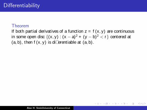
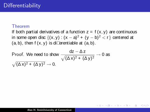
Differentiability
TheoremIf both partial derivatives of a function z = f (x , y) are continuousin some open disc {(x , y) : (x − a)2 + (y − b)2 < r} centered at(a, b), then f (x , y) is differentiable at (a, b).
Proof. We need to showdz −∆z√
(∆x)2 + (∆y)2→ 0 as√
(∆x)2 + (∆y)2 → 0.
We may write
∆z − dz = f (x , y)− f (a, b)−(
∂z
∂x(x − a) +
∂z
∂y(y − b)
)=
f (x , y)− f (a, y)− ∂z
∂x(x − a) + f (a, y)− f (a, b)− ∂z
∂y(y − b).
Alan H. SteinUniversity of Connecticut
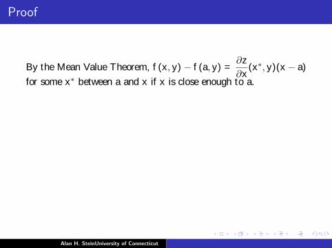
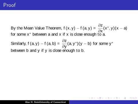
Proof
By the Mean Value Theorem, f (x , y)− f (a, y) =∂z
∂x(x∗, y)(x − a)
for some x∗ between a and x if x is close enough to a.
Similarly, f (a, y)− f (a, b) =∂z
∂y(a, y∗)(y − b) for some y∗
between b and y if y is close enough to b.
We thus get
∆z−dz =∂z
∂x(x∗, y)(x−a)− ∂z
∂x(x−a)+
∂z
∂y(a, y∗)(y−b)− ∂z
∂y(y−
b) =
(∂z
∂x(x∗, y)− ∂z
∂x
)(x − a) +
(∂z
∂x(a, y∗)− ∂z
∂y
)(y − b).
Alan H. SteinUniversity of Connecticut

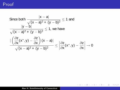
Proof
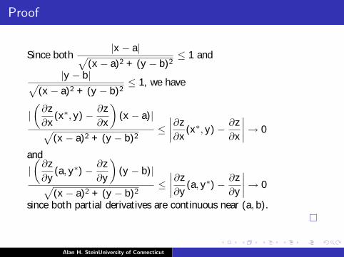
Since both|x − a|√
(x − a)2 + (y − b)2≤ 1 and
|y − b|√(x − a)2 + (y − b)2
≤ 1, we have
|(
∂z
∂x(x∗, y)− ∂z
∂x
)(x − a)|√
(x − a)2 + (y − b)2≤
∣∣∣∣∂z
∂x(x∗, y)− ∂z
∂x
∣∣∣∣ → 0
and
|(
∂z
∂y(a, y∗)− ∂z
∂y
)(y − b)|√
(x − a)2 + (y − b)2≤
∣∣∣∣∂z
∂y(a, y∗)− ∂z
∂y
∣∣∣∣ → 0
since both partial derivatives are continuous near (a, b).
Alan H. SteinUniversity of Connecticut
Proof
Since both|x − a|√
(x − a)2 + (y − b)2≤ 1 and
|y − b|√(x − a)2 + (y − b)2
≤ 1, we have
|(
∂z
∂x(x∗, y)− ∂z
∂x
)(x − a)|√
(x − a)2 + (y − b)2≤
∣∣∣∣∂z
∂x(x∗, y)− ∂z
∂x
∣∣∣∣ → 0
and
|(
∂z
∂y(a, y∗)− ∂z
∂y
)(y − b)|√
(x − a)2 + (y − b)2≤
∣∣∣∣∂z
∂y(a, y∗)− ∂z
∂y
∣∣∣∣ → 0
since both partial derivatives are continuous near (a, b).
Alan H. SteinUniversity of Connecticut

The Chain Rule
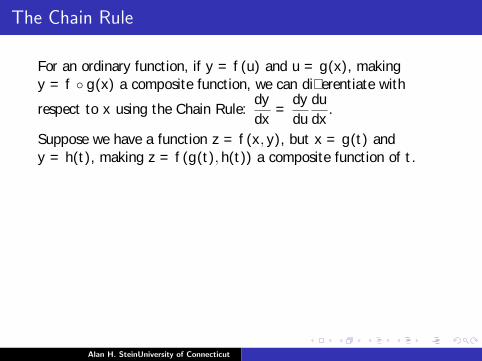
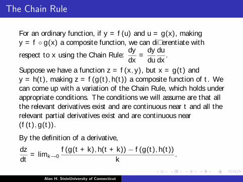
For an ordinary function, if y = f (u) and u = g(x), makingy = f ◦ g(x) a composite function, we can differentiate with
respect to x using the Chain Rule:dy
dx=
dy
du
du
dx.
Suppose we have a function z = f (x , y), but x = g(t) andy = h(t), making z = f (g(t), h(t)) a composite function of t. Wecan come up with a variation of the Chain Rule, which holds underappropriate conditions. The conditions we will assume are that allthe relevant derivatives exist and are continuous near t and all therelevant partial derivatives exist and are continuous near(f (t), g(t)).
By the definition of a derivative,
dz
dt= limk→0
f (g(t + k), h(t + k))− f (g(t), h(t))
k.
Alan H. SteinUniversity of Connecticut
The Chain Rule
For an ordinary function, if y = f (u) and u = g(x), makingy = f ◦ g(x) a composite function, we can differentiate with
respect to x using the Chain Rule:dy
dx=
dy
du
du
dx.
Suppose we have a function z = f (x , y), but x = g(t) andy = h(t), making z = f (g(t), h(t)) a composite function of t.
Wecan come up with a variation of the Chain Rule, which holds underappropriate conditions. The conditions we will assume are that allthe relevant derivatives exist and are continuous near t and all therelevant partial derivatives exist and are continuous near(f (t), g(t)).
By the definition of a derivative,
dz
dt= limk→0
f (g(t + k), h(t + k))− f (g(t), h(t))
k.
Alan H. SteinUniversity of Connecticut
The Chain Rule
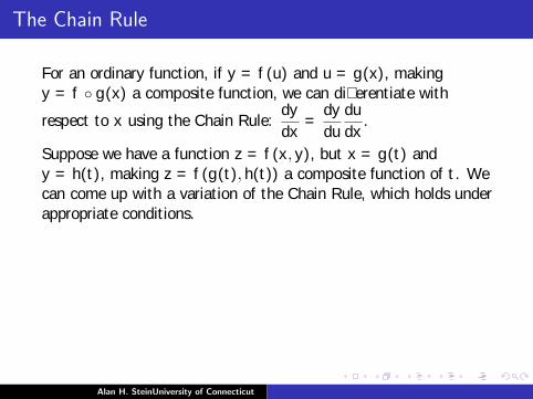
For an ordinary function, if y = f (u) and u = g(x), makingy = f ◦ g(x) a composite function, we can differentiate with
respect to x using the Chain Rule:dy
dx=
dy
du
du
dx.
Suppose we have a function z = f (x , y), but x = g(t) andy = h(t), making z = f (g(t), h(t)) a composite function of t. Wecan come up with a variation of the Chain Rule, which holds underappropriate conditions.
The conditions we will assume are that allthe relevant derivatives exist and are continuous near t and all therelevant partial derivatives exist and are continuous near(f (t), g(t)).
By the definition of a derivative,
dz
dt= limk→0
f (g(t + k), h(t + k))− f (g(t), h(t))
k.
Alan H. SteinUniversity of Connecticut
The Chain Rule
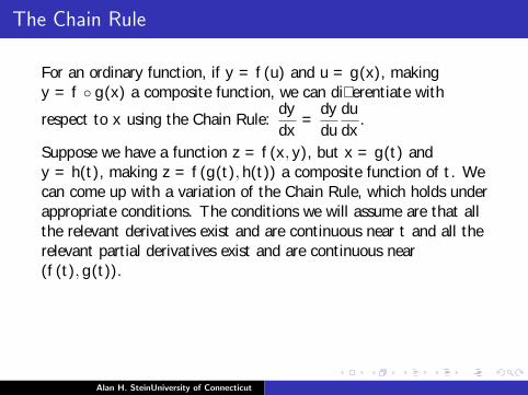
For an ordinary function, if y = f (u) and u = g(x), makingy = f ◦ g(x) a composite function, we can differentiate with
respect to x using the Chain Rule:dy
dx=
dy
du
du
dx.
Suppose we have a function z = f (x , y), but x = g(t) andy = h(t), making z = f (g(t), h(t)) a composite function of t. Wecan come up with a variation of the Chain Rule, which holds underappropriate conditions. The conditions we will assume are that allthe relevant derivatives exist and are continuous near t and all therelevant partial derivatives exist and are continuous near(f (t), g(t)).
By the definition of a derivative,
dz
dt= limk→0
f (g(t + k), h(t + k))− f (g(t), h(t))
k.
Alan H. SteinUniversity of Connecticut

The Chain Rule
For an ordinary function, if y = f (u) and u = g(x), makingy = f ◦ g(x) a composite function, we can differentiate with
respect to x using the Chain Rule:dy
dx=
dy
du
du
dx.
Suppose we have a function z = f (x , y), but x = g(t) andy = h(t), making z = f (g(t), h(t)) a composite function of t. Wecan come up with a variation of the Chain Rule, which holds underappropriate conditions. The conditions we will assume are that allthe relevant derivatives exist and are continuous near t and all therelevant partial derivatives exist and are continuous near(f (t), g(t)).
By the definition of a derivative,
dz
dt= limk→0
f (g(t + k), h(t + k))− f (g(t), h(t))
k.
Alan H. SteinUniversity of Connecticut
The Chain Rule
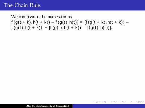
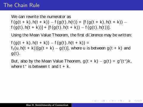
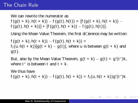
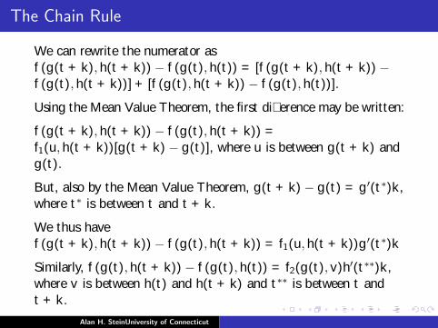
We can rewrite the numerator asf (g(t + k), h(t + k))− f (g(t), h(t)) = [f (g(t + k), h(t + k))−f (g(t), h(t + k))] + [f (g(t), h(t + k))− f (g(t), h(t))].
Using the Mean Value Theorem, the first difference may be written:
f (g(t + k), h(t + k))− f (g(t), h(t + k)) =f1(u, h(t + k))[g(t + k)− g(t)], where u is between g(t + k) andg(t).
But, also by the Mean Value Theorem, g(t + k)− g(t) = g ′(t∗)k,where t∗ is between t and t + k.
We thus havef (g(t + k), h(t + k))− f (g(t), h(t + k)) = f1(u, h(t + k))g ′(t∗)k
Similarly, f (g(t), h(t + k))− f (g(t), h(t)) = f2(g(t), v)h′(t∗∗)k,where v is between h(t) and h(t + k) and t∗∗ is between t andt + k.
Alan H. SteinUniversity of Connecticut

The Chain Rule
We can rewrite the numerator asf (g(t + k), h(t + k))− f (g(t), h(t)) = [f (g(t + k), h(t + k))−f (g(t), h(t + k))] + [f (g(t), h(t + k))− f (g(t), h(t))].
Using the Mean Value Theorem, the first difference may be written:
f (g(t + k), h(t + k))− f (g(t), h(t + k)) =f1(u, h(t + k))[g(t + k)− g(t)], where u is between g(t + k) andg(t).
But, also by the Mean Value Theorem, g(t + k)− g(t) = g ′(t∗)k,where t∗ is between t and t + k.
We thus havef (g(t + k), h(t + k))− f (g(t), h(t + k)) = f1(u, h(t + k))g ′(t∗)k
Similarly, f (g(t), h(t + k))− f (g(t), h(t)) = f2(g(t), v)h′(t∗∗)k,where v is between h(t) and h(t + k) and t∗∗ is between t andt + k.
Alan H. SteinUniversity of Connecticut
The Chain Rule
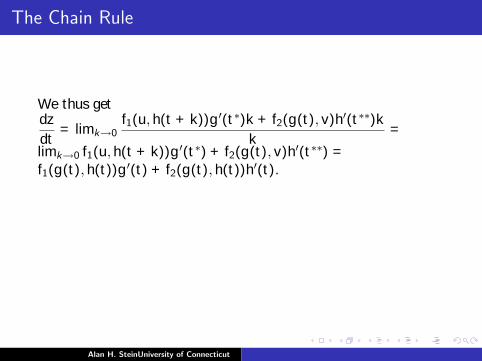
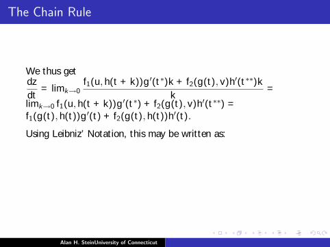
We thus getdz
dt= limk→0
f1(u, h(t + k))g ′(t∗)k + f2(g(t), v)h′(t∗∗)k
k=
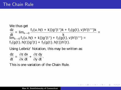
limk→0 f1(u, h(t + k))g ′(t∗) + f2(g(t), v)h′(t∗∗) =f1(g(t), h(t))g ′(t) + f2(g(t), h(t))h′(t).
Using Leibniz’ Notation, this may be written as:
dz
dt=
∂z
∂x
dx
dt+
∂z
∂y
dy
dt.
This is one variation of the Chain Rule.
Alan H. SteinUniversity of Connecticut
The Chain Rule
We thus getdz
dt= limk→0
f1(u, h(t + k))g ′(t∗)k + f2(g(t), v)h′(t∗∗)k
k=
limk→0 f1(u, h(t + k))g ′(t∗) + f2(g(t), v)h′(t∗∗) =f1(g(t), h(t))g ′(t) + f2(g(t), h(t))h′(t).
Using Leibniz’ Notation, this may be written as:
dz
dt=
∂z
∂x
dx
dt+
∂z
∂y
dy
dt.
This is one variation of the Chain Rule.
Alan H. SteinUniversity of Connecticut
Partial Derivatives Via the Chain Rule
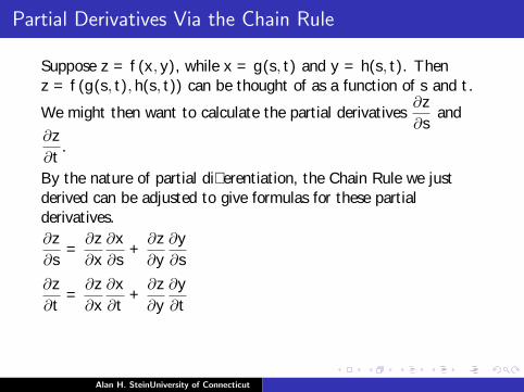
Suppose z = f (x , y), while x = g(s, t) and y = h(s, t).
Thenz = f (g(s, t), h(s, t)) can be thought of as a function of s and t.
We might then want to calculate the partial derivatives∂z
∂sand
∂z
∂t.
By the nature of partial differentiation, the Chain Rule we justderived can be adjusted to give formulas for these partialderivatives.
∂z
∂s=
∂z
∂x
∂x
∂s+
∂z
∂y
∂y
∂s
∂z
∂t=
∂z
∂x
∂x
∂t+
∂z
∂y
∂y
∂t
If we have functions involving more than two variables, this may beadjusted in the hopefully obvious way.
Alan H. SteinUniversity of Connecticut
Partial Derivatives Via the Chain Rule
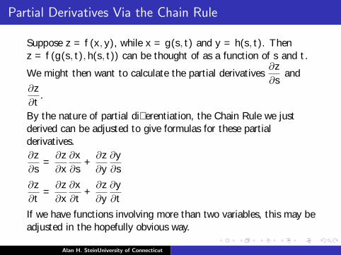
Suppose z = f (x , y), while x = g(s, t) and y = h(s, t). Thenz = f (g(s, t), h(s, t)) can be thought of as a function of s and t.
We might then want to calculate the partial derivatives∂z
∂sand
∂z
∂t.
By the nature of partial differentiation, the Chain Rule we justderived can be adjusted to give formulas for these partialderivatives.
∂z
∂s=
∂z
∂x
∂x
∂s+
∂z
∂y
∂y
∂s
∂z
∂t=
∂z
∂x
∂x
∂t+
∂z
∂y
∂y
∂t
If we have functions involving more than two variables, this may beadjusted in the hopefully obvious way.
Alan H. SteinUniversity of Connecticut
Partial Derivatives Via the Chain Rule
Suppose z = f (x , y), while x = g(s, t) and y = h(s, t). Thenz = f (g(s, t), h(s, t)) can be thought of as a function of s and t.
We might then want to calculate the partial derivatives∂z
∂sand
∂z
∂t.
By the nature of partial differentiation, the Chain Rule we justderived can be adjusted to give formulas for these partialderivatives.
∂z
∂s=
∂z
∂x
∂x
∂s+
∂z
∂y
∂y
∂s
∂z
∂t=
∂z
∂x
∂x
∂t+
∂z
∂y
∂y
∂t
If we have functions involving more than two variables, this may beadjusted in the hopefully obvious way.
Alan H. SteinUniversity of Connecticut
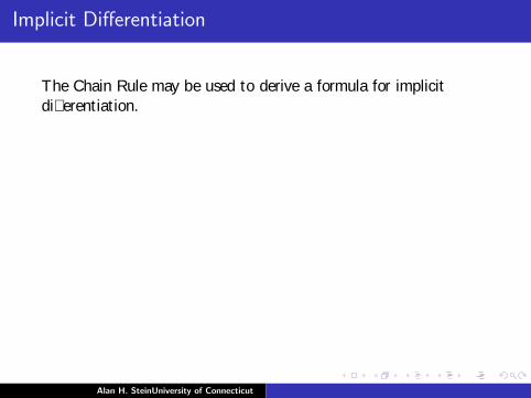
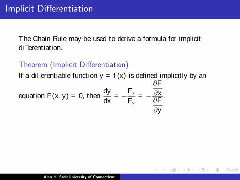
Implicit Differentiation
The Chain Rule may be used to derive a formula for implicitdifferentiation.
Theorem (Implicit Differentiation)
If a differentiable function y = f (x) is defined implicitly by an
equation F (x , y) = 0, thendy
dx= −Fx
Fy= −
∂F
∂x∂F
∂y
.
Note: We have assumed y = f (x) is differentiable. We are nothere dealing with how one knows whether such a function isdifferentiable. In general, if such a function is not differentiable, itwill be relatively obvious.
Alan H. SteinUniversity of Connecticut
Implicit Differentiation
The Chain Rule may be used to derive a formula for implicitdifferentiation.
Theorem (Implicit Differentiation)
If a differentiable function y = f (x) is defined implicitly by an
equation F (x , y) = 0, thendy
dx= −Fx
Fy= −
∂F
∂x∂F
∂y
.
Note: We have assumed y = f (x) is differentiable.
We are nothere dealing with how one knows whether such a function isdifferentiable. In general, if such a function is not differentiable, itwill be relatively obvious.
Alan H. SteinUniversity of Connecticut
Implicit Differentiation
The Chain Rule may be used to derive a formula for implicitdifferentiation.
Theorem (Implicit Differentiation)
If a differentiable function y = f (x) is defined implicitly by an
equation F (x , y) = 0, thendy
dx= −Fx
Fy= −
∂F
∂x∂F
∂y
.
Note: We have assumed y = f (x) is differentiable. We are nothere dealing with how one knows whether such a function isdifferentiable.
In general, if such a function is not differentiable, itwill be relatively obvious.
Alan H. SteinUniversity of Connecticut
Implicit Differentiation
The Chain Rule may be used to derive a formula for implicitdifferentiation.
Theorem (Implicit Differentiation)
If a differentiable function y = f (x) is defined implicitly by an
equation F (x , y) = 0, thendy
dx= −Fx
Fy= −
∂F
∂x∂F
∂y
.
Note: We have assumed y = f (x) is differentiable. We are nothere dealing with how one knows whether such a function isdifferentiable. In general, if such a function is not differentiable, itwill be relatively obvious.
Alan H. SteinUniversity of Connecticut
Implicit Differentiation
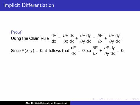
Proof.
Using the Chain Rule,dF
dx=
∂F
∂x
dx
dx+
∂F
∂y
dy
dx=
∂F
∂x+
∂F
∂y
dy
dx.
Since F (x , y) = 0, it follows thatdF
dx= 0, so
∂F
∂x+
∂F
∂y
dy
dx= 0.
Solving fordy
dx, we get
∂F
∂y
dy
dx= −∂F
∂x, so
dy
dx= −
∂F
∂x∂F
∂y
.
Alan H. SteinUniversity of Connecticut

Implicit Differentiation
Proof.
Using the Chain Rule,dF
dx=
∂F
∂x
dx
dx+
∂F
∂y
dy
dx=
∂F
∂x+
∂F
∂y
dy
dx.
Since F (x , y) = 0,
it follows thatdF
dx= 0, so
∂F
∂x+
∂F
∂y
dy
dx= 0.
Solving fordy
dx, we get
∂F
∂y
dy
dx= −∂F
∂x, so
dy
dx= −
∂F
∂x∂F
∂y
.
Alan H. SteinUniversity of Connecticut

Implicit Differentiation
Proof.
Using the Chain Rule,dF
dx=
∂F
∂x
dx
dx+
∂F
∂y
dy
dx=
∂F
∂x+
∂F
∂y
dy
dx.
Since F (x , y) = 0, it follows thatdF
dx= 0,
so∂F
∂x+
∂F
∂y
dy
dx= 0.
Solving fordy
dx, we get
∂F
∂y
dy
dx= −∂F
∂x, so
dy
dx= −
∂F
∂x∂F
∂y
.
Alan H. SteinUniversity of Connecticut
Implicit Differentiation
Proof.
Using the Chain Rule,dF
dx=
∂F
∂x
dx
dx+
∂F
∂y
dy
dx=
∂F
∂x+
∂F
∂y
dy
dx.
Since F (x , y) = 0, it follows thatdF
dx= 0, so
∂F
∂x+
∂F
∂y
dy
dx= 0.
Solving fordy
dx, we get
∂F
∂y
dy
dx= −∂F
∂x, so
dy
dx= −
∂F
∂x∂F
∂y
.
Alan H. SteinUniversity of Connecticut

Implicit Differentiation
Proof.
Using the Chain Rule,dF
dx=
∂F
∂x
dx
dx+
∂F
∂y
dy
dx=
∂F
∂x+
∂F
∂y
dy
dx.
Since F (x , y) = 0, it follows thatdF
dx= 0, so
∂F
∂x+
∂F
∂y
dy
dx= 0.
Solving fordy
dx, we get
∂F
∂y
dy
dx= −∂F
∂x,
sody
dx= −
∂F
∂x∂F
∂y
.
Alan H. SteinUniversity of Connecticut

Implicit Differentiation
Proof.
Using the Chain Rule,dF
dx=
∂F
∂x
dx
dx+
∂F
∂y
dy
dx=
∂F
∂x+
∂F
∂y
dy
dx.
Since F (x , y) = 0, it follows thatdF
dx= 0, so
∂F
∂x+
∂F
∂y
dy
dx= 0.
Solving fordy
dx, we get
∂F
∂y
dy
dx= −∂F
∂x, so
dy
dx= −
∂F
∂x∂F
∂y
.
Alan H. SteinUniversity of Connecticut
Directional Derivatives
Consider a function z = f (x , y) and its graph, which will be asurface.
The partial derivative∂z
∂xmay be thought of as representing how
fast the surface is rising above one’s head if one is walking on thexy -plane in the direction of the x-axis.
Similarly, the partial derivative∂z
∂ymay be thought of as
representing how fast the surface is rising above one’s head if oneis walking on the xy -plane in the direction of the y -axis.
Alan H. SteinUniversity of Connecticut

Directional Derivative
For a given unit vector u, we define the directional derivative Duzto represent how fast the surface is rising above one’s head if oneis walking on the xy -plane in the direction of u.
Definition (Directional Derivative)
Let f : Rn → R and let u ∈ Rn be a unit vector. Letg(t) = f (x + ut). Duf (x) = g ′(0) is called the directionalderivative of f at x in the direction of u.
Note that if n = 1, then the directional derivative is the same asthe ordinary derivative, while the directional derivatives in thedirections of the coordinate axes are the same as the partialderivatives.
Alan H. SteinUniversity of Connecticut
The Del Operator and the Gradient
Definition (Del Operator)
5 =
(∂
∂x,
∂
∂y
)
Note this is really just a symbolic entity. By itself, it ismeaningless, but we use it as a mneumonic device.
Definition (Gradient)
grad f = 5f =
(∂f
∂x,∂f
∂y
)The gradient turns out to be convenient when calculatingdirectional derivatives. It also generalizes to higher dimensions.
Alan H. SteinUniversity of Connecticut
The Del Operator and the Gradient
Definition (Del Operator)
5 =
(∂
∂x,
∂
∂y
)Note this is really just a symbolic entity. By itself, it ismeaningless, but we use it as a mneumonic device.
Definition (Gradient)
grad f = 5f =
(∂f
∂x,∂f
∂y
)The gradient turns out to be convenient when calculatingdirectional derivatives. It also generalizes to higher dimensions.
Alan H. SteinUniversity of Connecticut

The Del Operator and the Gradient
Definition (Del Operator)
5 =
(∂
∂x,
∂
∂y
)Note this is really just a symbolic entity. By itself, it ismeaningless, but we use it as a mneumonic device.
Definition (Gradient)
grad f = 5f =
(∂f
∂x,∂f
∂y
)
The gradient turns out to be convenient when calculatingdirectional derivatives. It also generalizes to higher dimensions.
Alan H. SteinUniversity of Connecticut
The Del Operator and the Gradient
Definition (Del Operator)
5 =
(∂
∂x,
∂
∂y
)Note this is really just a symbolic entity. By itself, it ismeaningless, but we use it as a mneumonic device.
Definition (Gradient)
grad f = 5f =
(∂f
∂x,∂f
∂y
)The gradient turns out to be convenient when calculatingdirectional derivatives.
It also generalizes to higher dimensions.
Alan H. SteinUniversity of Connecticut

The Del Operator and the Gradient
Definition (Del Operator)
5 =
(∂
∂x,
∂
∂y
)Note this is really just a symbolic entity. By itself, it ismeaningless, but we use it as a mneumonic device.
Definition (Gradient)
grad f = 5f =
(∂f
∂x,∂f
∂y
)The gradient turns out to be convenient when calculatingdirectional derivatives. It also generalizes to higher dimensions.
Alan H. SteinUniversity of Connecticut

Calculating Directional Derivatives
TheoremIf all the partial derivatives of z = f (x) are continuous is someopen ball centered at x, then Duf (x) = (5f ) · u.
This theorem gives us a convenient way to calculate any directionalderivative of a function and also shows that it is sufficient to beable to calculate all the partial derivatives.
Alan H. SteinUniversity of Connecticut
Proof
We will prove the theorem for R2, but a similar proof will work forhigher dimensions; only the notation would get messier.
Proof.Consider a function f (x , y) and a unit vector u =< a, b >. Letz = g(t) be defined by letting z = f (x , y), where x = x0 + at,y = y0 + bt.
By definition, Duf (x0, y0) = g ′(0).
By the Chain Rule, g ′(t) =dz
dt=
∂z
∂x
dx
dt+
∂z
∂y
dy
dt= (5z) · u.
Evaluating this at 0 gives the result.
Alan H. SteinUniversity of Connecticut
Maximum Value of the Directional Derivative
Duf = (5f ) · u = |5f | |u| cos θ, where θ is the angle between 5fand u.
Since −1 ≤ cos θ ≤ 1, the maximal value obviously occurs whenθ = 0 and cos θ = 1, in other words, when u is in the samedirection as 5f .
There’s a catch: This depends on the property u · v = |u||v| cos θ,which we’ve seen for R2 and R3, but whose very meaning isunclear for higher dimensions.
Alan H. SteinUniversity of Connecticut
Maximum Value of the Directional Derivative
Duf = (5f ) · u = |5f | |u| cos θ, where θ is the angle between 5fand u.
Since −1 ≤ cos θ ≤ 1, the maximal value obviously occurs whenθ = 0 and cos θ = 1,
in other words, when u is in the samedirection as 5f .
There’s a catch: This depends on the property u · v = |u||v| cos θ,which we’ve seen for R2 and R3, but whose very meaning isunclear for higher dimensions.
Alan H. SteinUniversity of Connecticut

Maximum Value of the Directional Derivative
Duf = (5f ) · u = |5f | |u| cos θ, where θ is the angle between 5fand u.
Since −1 ≤ cos θ ≤ 1, the maximal value obviously occurs whenθ = 0 and cos θ = 1, in other words, when u is in the samedirection as 5f .
There’s a catch: This depends on the property u · v = |u||v| cos θ,which we’ve seen for R2 and R3, but whose very meaning isunclear for higher dimensions.
Alan H. SteinUniversity of Connecticut
Maximum Value of the Directional Derivative
Duf = (5f ) · u = |5f | |u| cos θ, where θ is the angle between 5fand u.
Since −1 ≤ cos θ ≤ 1, the maximal value obviously occurs whenθ = 0 and cos θ = 1, in other words, when u is in the samedirection as 5f .
There’s a catch:
This depends on the property u · v = |u||v| cos θ,which we’ve seen for R2 and R3, but whose very meaning isunclear for higher dimensions.
Alan H. SteinUniversity of Connecticut
Maximum Value of the Directional Derivative
Duf = (5f ) · u = |5f | |u| cos θ, where θ is the angle between 5fand u.
Since −1 ≤ cos θ ≤ 1, the maximal value obviously occurs whenθ = 0 and cos θ = 1, in other words, when u is in the samedirection as 5f .
There’s a catch: This depends on the property u · v = |u||v| cos θ,
which we’ve seen for R2 and R3, but whose very meaning isunclear for higher dimensions.
Alan H. SteinUniversity of Connecticut

Maximum Value of the Directional Derivative
Duf = (5f ) · u = |5f | |u| cos θ, where θ is the angle between 5fand u.
Since −1 ≤ cos θ ≤ 1, the maximal value obviously occurs whenθ = 0 and cos θ = 1, in other words, when u is in the samedirection as 5f .
There’s a catch: This depends on the property u · v = |u||v| cos θ,which we’ve seen for R2 and R3, but whose very meaning isunclear for higher dimensions.
Alan H. SteinUniversity of Connecticut
Cauchy-Schwarz Inequality
We can give u · v = |u||v| cos θ meaning through theCauchy-Schwarz Inequality u · v ≤ |u||v|.
We will show theCauchy-Schwarz Inequality holds in any dimension, with equalityholding if and only if one vector is a multiple of the other.
Consider a vector u− tv. Certainly (u− tv) · (u− tv) ≥ 0, withequality holding if and only if u is a multiple t of v or v = 0.
Since(u− tv) · (u− tv) = u · u− 2tu · v + t2vv = |v|2t2 − 2u · vt + |u|2,we get |v|2t2 − 2u · vt + |u|2 ≥ 0.
Alan H. SteinUniversity of Connecticut
Cauchy-Schwarz Inequality
We can give u · v = |u||v| cos θ meaning through theCauchy-Schwarz Inequality u · v ≤ |u||v|. We will show theCauchy-Schwarz Inequality holds in any dimension, with equalityholding if and only if one vector is a multiple of the other.
Consider a vector u− tv. Certainly (u− tv) · (u− tv) ≥ 0, withequality holding if and only if u is a multiple t of v or v = 0.
Since(u− tv) · (u− tv) = u · u− 2tu · v + t2vv = |v|2t2 − 2u · vt + |u|2,we get |v|2t2 − 2u · vt + |u|2 ≥ 0.
Alan H. SteinUniversity of Connecticut

Cauchy-Schwarz Inequality
We can give u · v = |u||v| cos θ meaning through theCauchy-Schwarz Inequality u · v ≤ |u||v|. We will show theCauchy-Schwarz Inequality holds in any dimension, with equalityholding if and only if one vector is a multiple of the other.
Consider a vector u− tv. Certainly (u− tv) · (u− tv) ≥ 0, withequality holding if and only if u is a multiple t of v or v = 0.
Since(u− tv) · (u− tv) = u · u− 2tu · v + t2vv = |v|2t2 − 2u · vt + |u|2,
we get |v|2t2 − 2u · vt + |u|2 ≥ 0.
Alan H. SteinUniversity of Connecticut
Cauchy-Schwarz Inequality
We can give u · v = |u||v| cos θ meaning through theCauchy-Schwarz Inequality u · v ≤ |u||v|. We will show theCauchy-Schwarz Inequality holds in any dimension, with equalityholding if and only if one vector is a multiple of the other.
Consider a vector u− tv. Certainly (u− tv) · (u− tv) ≥ 0, withequality holding if and only if u is a multiple t of v or v = 0.
Since(u− tv) · (u− tv) = u · u− 2tu · v + t2vv = |v|2t2 − 2u · vt + |u|2,we get |v|2t2 − 2u · vt + |u|2 ≥ 0.
Alan H. SteinUniversity of Connecticut

Cauchy-Schwarz Inequality
It follows that the quadratic equation |v|2t2 − 2u · vt + |u|2 = 0 int can’t have more than one solution,
so the discriminant(−2u · v)2 − 4|v|2|u|2 can’t be positive.
In other words, (−2u · v)2 − 4|v|2|u|2 ≤ 0, so4(u · v)2 − 4|v|2|u|2 ≤ 0, so (u · v)2 − |v|2|u|2 ≤ 0, so(u · v)2 ≤ |v|2|u|2, so u · v ≤ |u||v|.
Equality clearly holds if and only if either u− tv = 0 or if v = 0, inother words, if and only if either u is a scalar multiple of v or ifv = 0.
Alan H. SteinUniversity of Connecticut
Cauchy-Schwarz Inequality
It follows that the quadratic equation |v|2t2 − 2u · vt + |u|2 = 0 int can’t have more than one solution, so the discriminant(−2u · v)2 − 4|v|2|u|2 can’t be positive.
In other words, (−2u · v)2 − 4|v|2|u|2 ≤ 0,
so4(u · v)2 − 4|v|2|u|2 ≤ 0, so (u · v)2 − |v|2|u|2 ≤ 0, so(u · v)2 ≤ |v|2|u|2, so u · v ≤ |u||v|.
Equality clearly holds if and only if either u− tv = 0 or if v = 0, inother words, if and only if either u is a scalar multiple of v or ifv = 0.
Alan H. SteinUniversity of Connecticut
Cauchy-Schwarz Inequality
It follows that the quadratic equation |v|2t2 − 2u · vt + |u|2 = 0 int can’t have more than one solution, so the discriminant(−2u · v)2 − 4|v|2|u|2 can’t be positive.
In other words, (−2u · v)2 − 4|v|2|u|2 ≤ 0, so4(u · v)2 − 4|v|2|u|2 ≤ 0,
so (u · v)2 − |v|2|u|2 ≤ 0, so(u · v)2 ≤ |v|2|u|2, so u · v ≤ |u||v|.
Equality clearly holds if and only if either u− tv = 0 or if v = 0, inother words, if and only if either u is a scalar multiple of v or ifv = 0.
Alan H. SteinUniversity of Connecticut
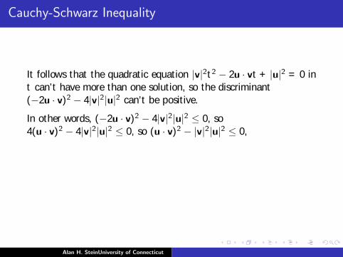
Cauchy-Schwarz Inequality
It follows that the quadratic equation |v|2t2 − 2u · vt + |u|2 = 0 int can’t have more than one solution, so the discriminant(−2u · v)2 − 4|v|2|u|2 can’t be positive.
In other words, (−2u · v)2 − 4|v|2|u|2 ≤ 0, so4(u · v)2 − 4|v|2|u|2 ≤ 0, so (u · v)2 − |v|2|u|2 ≤ 0,
so(u · v)2 ≤ |v|2|u|2, so u · v ≤ |u||v|.
Equality clearly holds if and only if either u− tv = 0 or if v = 0, inother words, if and only if either u is a scalar multiple of v or ifv = 0.
Alan H. SteinUniversity of Connecticut

Cauchy-Schwarz Inequality
It follows that the quadratic equation |v|2t2 − 2u · vt + |u|2 = 0 int can’t have more than one solution, so the discriminant(−2u · v)2 − 4|v|2|u|2 can’t be positive.
In other words, (−2u · v)2 − 4|v|2|u|2 ≤ 0, so4(u · v)2 − 4|v|2|u|2 ≤ 0, so (u · v)2 − |v|2|u|2 ≤ 0, so(u · v)2 ≤ |v|2|u|2,
so u · v ≤ |u||v|.
Equality clearly holds if and only if either u− tv = 0 or if v = 0, inother words, if and only if either u is a scalar multiple of v or ifv = 0.
Alan H. SteinUniversity of Connecticut

Cauchy-Schwarz Inequality
It follows that the quadratic equation |v|2t2 − 2u · vt + |u|2 = 0 int can’t have more than one solution, so the discriminant(−2u · v)2 − 4|v|2|u|2 can’t be positive.
In other words, (−2u · v)2 − 4|v|2|u|2 ≤ 0, so4(u · v)2 − 4|v|2|u|2 ≤ 0, so (u · v)2 − |v|2|u|2 ≤ 0, so(u · v)2 ≤ |v|2|u|2, so u · v ≤ |u||v|.
Equality clearly holds if and only if either u− tv = 0 or if v = 0, inother words, if and only if either u is a scalar multiple of v or ifv = 0.
Alan H. SteinUniversity of Connecticut
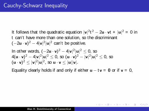
Cauchy-Schwarz Inequality
It follows that the quadratic equation |v|2t2 − 2u · vt + |u|2 = 0 int can’t have more than one solution, so the discriminant(−2u · v)2 − 4|v|2|u|2 can’t be positive.
In other words, (−2u · v)2 − 4|v|2|u|2 ≤ 0, so4(u · v)2 − 4|v|2|u|2 ≤ 0, so (u · v)2 − |v|2|u|2 ≤ 0, so(u · v)2 ≤ |v|2|u|2, so u · v ≤ |u||v|.
Equality clearly holds if and only if either u− tv = 0 or if v = 0,
inother words, if and only if either u is a scalar multiple of v or ifv = 0.
Alan H. SteinUniversity of Connecticut

Cauchy-Schwarz Inequality
It follows that the quadratic equation |v|2t2 − 2u · vt + |u|2 = 0 int can’t have more than one solution, so the discriminant(−2u · v)2 − 4|v|2|u|2 can’t be positive.
In other words, (−2u · v)2 − 4|v|2|u|2 ≤ 0, so4(u · v)2 − 4|v|2|u|2 ≤ 0, so (u · v)2 − |v|2|u|2 ≤ 0, so(u · v)2 ≤ |v|2|u|2, so u · v ≤ |u||v|.
Equality clearly holds if and only if either u− tv = 0 or if v = 0, inother words, if and only if either u is a scalar multiple of v or ifv = 0.
Alan H. SteinUniversity of Connecticut

Cauchy-Schwarz and Directional Derivatives
Since |u · v| ≤ |u||v|,
it follows that −1 ≤ u · v|u||v|
≤ 1.
We may thus define the angle θ between u and v by
θ = arccos
(u · v|u||v|
).
It follows that u · v = |u||v| cos θ, so the argument we used beforeabout the directional derivative being maximal in the direction ofthe gradient can legitimately be used.
Alan H. SteinUniversity of Connecticut
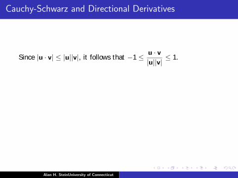
Cauchy-Schwarz and Directional Derivatives
Since |u · v| ≤ |u||v|, it follows that −1 ≤ u · v|u||v|
≤ 1.
We may thus define the angle θ between u and v by
θ = arccos
(u · v|u||v|
).
It follows that u · v = |u||v| cos θ, so the argument we used beforeabout the directional derivative being maximal in the direction ofthe gradient can legitimately be used.
Alan H. SteinUniversity of Connecticut
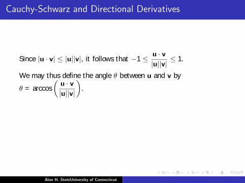
Cauchy-Schwarz and Directional Derivatives
Since |u · v| ≤ |u||v|, it follows that −1 ≤ u · v|u||v|
≤ 1.
We may thus define the angle θ between u and v by
θ = arccos
(u · v|u||v|
).
It follows that u · v = |u||v| cos θ,
so the argument we used beforeabout the directional derivative being maximal in the direction ofthe gradient can legitimately be used.
Alan H. SteinUniversity of Connecticut
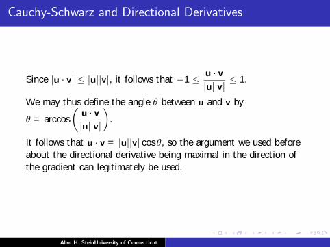
Cauchy-Schwarz and Directional Derivatives
Since |u · v| ≤ |u||v|, it follows that −1 ≤ u · v|u||v|
≤ 1.
We may thus define the angle θ between u and v by
θ = arccos
(u · v|u||v|
).
It follows that u · v = |u||v| cos θ, so the argument we used beforeabout the directional derivative being maximal in the direction ofthe gradient can legitimately be used.
Alan H. SteinUniversity of Connecticut
Tangent Planes and Gradients
Recall the formula for the plane tangent to the surface z = f (x , y)at a point (a, b):
z − c =∂z
∂x(x − a) +
∂z
∂y(y − b).
Using the language of gradients, this could be written in the formz − c = (5f )· < x − a, y − b > or z − c = (5f ) · (x− x0),where x =< x , y > and x0 =< a, b >.
Since one standard form for the equation of a plane isz − z0 = n · (x− x0), with n being a normal to the plane, it followsthat 5f is normal to the tangent plane.
Alan H. SteinUniversity of Connecticut
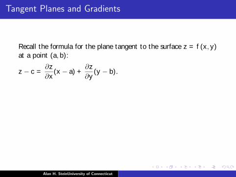
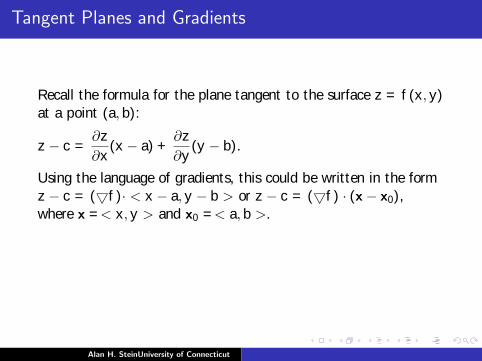
Tangent Planes and Gradients
Recall the formula for the plane tangent to the surface z = f (x , y)at a point (a, b):
z − c =∂z
∂x(x − a) +
∂z
∂y(y − b).
Using the language of gradients, this could be written in the formz − c = (5f )· < x − a, y − b > or z − c = (5f ) · (x− x0),where x =< x , y > and x0 =< a, b >.
Since one standard form for the equation of a plane isz − z0 = n · (x− x0), with n being a normal to the plane,
it followsthat 5f is normal to the tangent plane.
Alan H. SteinUniversity of Connecticut
Tangent Planes and Gradients
Recall the formula for the plane tangent to the surface z = f (x , y)at a point (a, b):
z − c =∂z
∂x(x − a) +
∂z
∂y(y − b).
Using the language of gradients, this could be written in the formz − c = (5f )· < x − a, y − b > or z − c = (5f ) · (x− x0),where x =< x , y > and x0 =< a, b >.
Since one standard form for the equation of a plane isz − z0 = n · (x− x0), with n being a normal to the plane, it followsthat 5f is normal to the tangent plane.
Alan H. SteinUniversity of Connecticut
Tangent Planes for Surfaces Defined Implicitly
Suppose a surface is the graph of an equation φ(x , y , z) = 0.
Atmost points (where there is a tangent plane and the tangent planeisn’t vertical), a portion of the surface near the point can beconsidered the graph of a function z = f (x , y) defined implicitly bythe equation φ(x , y , z) = 0 along with some side conditions.
Alan H. SteinUniversity of Connecticut
Tangent Planes for Surfaces Defined Implicitly
Suppose a surface is the graph of an equation φ(x , y , z) = 0. Atmost points (where there is a tangent plane and the tangent planeisn’t vertical), a portion of the surface near the point can beconsidered the graph of a function z = f (x , y) defined implicitly bythe equation φ(x , y , z) = 0 along with some side conditions.
Alan H. SteinUniversity of Connecticut
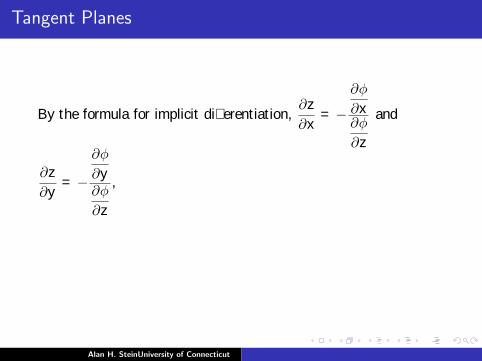
Tangent Planes
By the formula for implicit differentiation,∂z
∂x= −
∂φ
∂x∂φ
∂z
and
∂z
∂y= −
∂φ
∂y∂φ
∂z
,
so the equation of the tangent plane may be written
z − c = −
∂φ
∂x∂φ
∂z
(x − a)−
∂φ
∂y∂φ
∂z
(y − b).
Alan H. SteinUniversity of Connecticut

Tangent Planes
By the formula for implicit differentiation,∂z
∂x= −
∂φ
∂x∂φ
∂z
and
∂z
∂y= −
∂φ
∂y∂φ
∂z
, so the equation of the tangent plane may be written
z − c = −
∂φ
∂x∂φ
∂z
(x − a)−
∂φ
∂y∂φ
∂z
(y − b).
Alan H. SteinUniversity of Connecticut

Tangent Planes
z − c = −
∂φ
∂x∂φ
∂z
(x − a)−
∂φ
∂y∂φ
∂z
(y − b).
Simplifying:∂φ
∂z(z − c) = −∂φ
∂x(x − a)− ∂φ
∂y(y − b),
∂φ
∂x(x − a) +
∂φ
∂y(y − b) +
∂φ
∂z(z − c) = 0.
This can also be written in the form(5φ)· < x − a, y − b, z − c >= 0.
Alan H. SteinUniversity of Connecticut
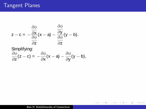
Tangent Planes
z − c = −
∂φ
∂x∂φ
∂z
(x − a)−
∂φ
∂y∂φ
∂z
(y − b).
Simplifying:∂φ
∂z(z − c) = −∂φ
∂x(x − a)− ∂φ
∂y(y − b),
∂φ
∂x(x − a) +
∂φ
∂y(y − b) +
∂φ
∂z(z − c) = 0.
This can also be written in the form(5φ)· < x − a, y − b, z − c >= 0.
Alan H. SteinUniversity of Connecticut
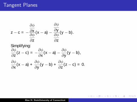
Tangent Planes
z − c = −
∂φ
∂x∂φ
∂z
(x − a)−
∂φ
∂y∂φ
∂z
(y − b).
Simplifying:∂φ
∂z(z − c) = −∂φ
∂x(x − a)− ∂φ
∂y(y − b),
∂φ
∂x(x − a) +
∂φ
∂y(y − b) +
∂φ
∂z(z − c) = 0.
This can also be written in the form(5φ)· < x − a, y − b, z − c >= 0.
Alan H. SteinUniversity of Connecticut
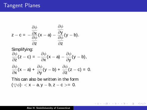
Tangent Planes
z − c = −
∂φ
∂x∂φ
∂z
(x − a)−
∂φ
∂y∂φ
∂z
(y − b).
Simplifying:∂φ
∂z(z − c) = −∂φ
∂x(x − a)− ∂φ
∂y(y − b),
∂φ
∂x(x − a) +
∂φ
∂y(y − b) +
∂φ
∂z(z − c) = 0.
This can also be written in the form(5φ)· < x − a, y − b, z − c >= 0.
Alan H. SteinUniversity of Connecticut