Extending Hypertextures toNon-Geometrically De�nable Volume

Data

Richard Satherley

Department of Computer Science

University of Wales, Swansea

Singleton Park

Swansea, UK

Mark Jones

Department of Computer Science

University of Wales, Swansea

Singleton Park

Swansea, UK

Abstract

Texture mapping is an extremely powerful tool for the addition of surfacedetail to an object. This paper aims to introduce the �eld of three dimen-sional texture mapping, in terms of "solid textures" and "hypertextures".The second half of the paper shows how the hypertexture paradigm canbe extended, with the use of "distance transforms", to incorporate non-geometrically de�nable datasets.

1 Introduction

The increasing use of computer generated graphical representations of everyday

objects, in both entertainment and industry (including such areas as medical

imaging), has led to the development of powerful rendering tools such as ray

tracing, radiosity and volume rendering (see [1,2] for a description). However,

the images produced by such applications are somewhat bland when compared

to their real life counterparts. The object's surfaces appears smooth and plastic

(Figure 1), not textured and natural. Therefore, increased realism in computer

imagery is needed.

Figure 1: Computer generated images.

Such realism can be incorporated into a computer generated image with the

application of "surface detail" algorithms, including:

� Bump mapping,

� Environment mapping, and

� Texture mapping in one, two and three dimensions.

Two dimensional texture maps are the more diverse of the "surface de-

tail" algorithms as, with the use of digitised photographs, natural textures can

be used. However this approach su�ers from aliasing e�ects (caused by the

warping of the texture) when applied to complex datasets, such as those ob-

tained from computerised tomography (CT) scans. Three dimensional texture

mapping techniques are more resistant to such aliasing e�ects, as the need for

image warping is removed by the fact that the texture map is mathematically

de�ned throughout R3 , thus any point on the surface of the rendered object

has a prede�ned texture value. Therefore, the 3D texture mapping approach

is analogous to carving a statue from a block of material, Figure 2.

Texture block Textured object

Figure 2: Three dimensional texture mapping.

Perlin and Ho�ert [3] extended the three dimensional texture mapping

paradigm to produce "hypertextures", allowing a computer to model such phe-

nomena as fur, �re and smoke. This paper shows how hypertextures can be

extended to use with non-geometrical datasets. In Section 2 we introduce the

area of three dimensional texture mapping through solid textures, followed by

a description of hypertextures in Section 3. Finally in Section 4.1 we show

how a volume dataset is modi�ed with the use of distance transforms, thus

allowing the application of the hypertexture model. Section 4.2 shows images

produced with extended hypertextures, and Section 4.3 shows how the extended

hypertextures produce images that are consistent, allowing the production of

animations.

2 Solid Texturing

2.1 Related Work

Recent trends in research into the addition of detail to the surface of an object

have turned towards the �eld of three dimensional texture mapping. Early

work in this �eld, such as that by Schachter [4], used summations of long

crested narrow-band noise waveforms to produce textures, that vary in two

dimensions, by Fourier synthesis.

Peachey [5] shows how popular two dimensional texturing techniques, such

as Fourier synthesis and stochastic texture models, can be extended to produce

three dimensional textures. Combinations of these extended techniques, along

with 3D projections of 2D images, make up what Peachey coined "solid tex-

tures". Perlin also used the term solid textures to describe the work in [6]. Here

complex three dimensional textures, such as marble, are created from primi-

tive, non-linear, "basis functions". The most fundamental of which is "noise",

a function that returns a random value at each point in space. In [7] Lewis

reviews several existing algorithms for noise generation, resulting in two new

algorithms that are more eÆcient, have improved control over the noise power

spectrum, and have no artifacts. A further basis function, introduced by Wor-

ley in [8], creates agstone-like textures by calculating the distance between

the surface points and randomly placed "feature points".

As mentioned above Peachey projects a digitised 2D image in order to create

a 3D texture. A problem arises when the object is larger than the texture,

resulting in the need for texture repetition, which can lead to visible artifacts

between the texture tiles. Research into texture analysis aims to remove such

e�ects by synthesising a new texture (of any size), that looks like (in terms of

colour and texture properties) a given sample image.

Heeger and Bergen [9] base their analysis around the way in which the eye

perceives texture, utalising the fact that it is diÆcult to discriminate between

textures that produce similar responses in a bank of linear �lters. Therefore,

with the application of simple image processing operations (histograms, convo-

lution, etc.), in a pyramidal format, white noise can be modi�ed to take on the

appearance of a sample image.

Solid textures produced by Heeger and Bergen's method can be imagined

as a stack of "photocopies", with each layer being an exact copy of the one

below. Ghazanfarpour and Dischler [10] use some of the spectral information,

gained during the analysis of the sample image, to apply a selective �lter to

white noise. The �ltered noise is next used to perturb the layers of the synthe-

sised texture, thus removing the monotony of Heeger and Bergen's method and

creating far more realistic solid textures. In a second paper [11] Ghazanfarpour

and Dischler show that solid textures synthesised from a single 2D sample are

only controllable in two dimensions. They continue to show that with the use

of three samples, taken in the directions of the orthogonal axes, it is possible

to control the texture synthesis in all three dimensions.

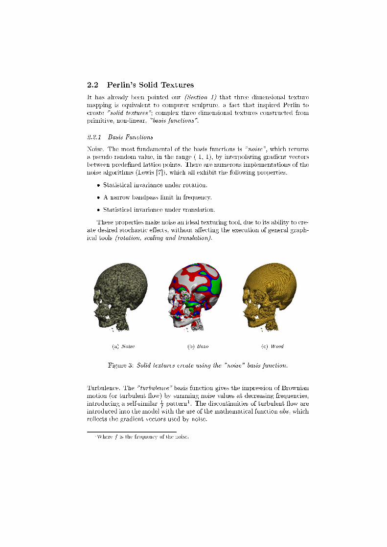
2.2 Perlin's Solid Textures

It has already been pointed out (Section 1) that three dimensional texture

mapping is equivalent to computer sculpture, a fact that inspired Perlin to

create "solid textures"; complex three dimensional textures constructed from

primitive, non-linear, "basis functions".

2.2.1 Basis Functions

Noise. The most fundamental of the basis functions is "noise", which returns

a pseudo-random value, in the range (-1, 1), by interpolating gradient vectors

between prede�ned lattice points. There are numerous implementations of the

noise algorithms (Lewis [7]), which all exhibit the following properties.

� Statistical invariance under rotation.

� A narrow bandpass limit in frequency.

� Statistical invariance under translation.

These properties make noise an ideal texturing tool, due to its ability to cre-

ate desired stochastic e�ects, without a�ecting the execution of general graph-

ical tools (rotation, scaling and translation).

(a) Noise (b) Bozo (c) Wood

Figure 3: Solid textures create using the "noise" basis function.

Turbulence. The "turbulence" basis function gives the impression of Brownian

motion (or turbulent ow) by summing noise values at decreasing frequencies,

introducing a self-similar 1

fpattern1. The discontinuities of turbulent ow are

introduced into the model with the use of the mathematical function abs, which

re ects the gradient vectors used by noise.

1Where f is the frequency of the noise.

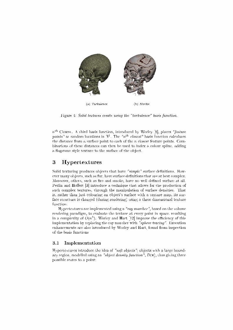
(a) Turbulence (b) Marble

Figure 4: Solid textures create using the "turbulence" basis function.

nth Closest. A third basis function, introduced by Worley [8], places "feature

points" at random locations in R3 . The "nth closest" basis function calculates

the distance from a surface point to each of the n closest feature points. Com-

binations of these distances can then be used to index a colour spline, adding

a agstone style texture to the surface of the object.

3 Hypertextures

Solid texturing produces objects that have "simple" surface de�nitions. How-

ever many objects, such as fur, have surface de�nitions that are at best complex.

Moreover, others, such as �re and smoke, have no well de�ned surface at all.

Perlin and Ho�ert [3] introduce a technique that allows for the production of

such complex textures, through the manipulation of surface densities. That

is, rather than just colouring an object's surface with a texture map, its sur-

face structure is changed (during rendering) using a three dimensional texture

function.

Hypertextures are implemented using a "ray marcher", based on the volume

rendering paradigm, to evaluate the texture at every point in space, resulting

in a complexity of O(n3). Worley and Hart [12] improve the eÆciency of this

implementation by replacing the ray marcher with "sphere tracing". Execution

enhancements are also introduced by Worley and Hart, found from inspection

of the basis functions

3.1 Implementation

Hypertextures introduce the idea of "soft objects"; objects with a large bound-

ary region, modelled using an "object density function", D(x), thus giving three

possible states to a point:

� Inside - the point is inside the object.

� Outside - the point is outside of the object.

� Boundary - the point is in the boundary, "soft", region of the object.

As with solid textures, combinations of noise and turbulence (Section 2)

together with two new density modulation functions (DMF), bias; controls the

density variation across the soft region, and gain; controls the rate at which

density changes across the midrange of the soft region, are used to manipulate

D(x) to create hypertextured objects. Figure 5 shows examples of hypertex-

tured objects.

(a) Noisy sphere (b) Melting sphere (c) Fireball

(d) Ring of �re (e) Straight fur (f) Curly fur

Figure 5: Examples of hypertextures.

4 Extending Hypertextures

Figure 5 shows the pleasing e�ects that can be produced when the hypertex-

ture approach is applied to geometrically de�nable datasets. The major set

back with this approach is the inability to apply the method to irregular (or

non-geometrically de�nable) datasets, such as CT scans.

4.1 Distance Transforms

Examination of datasets, generated by solving geometric formulae, shows that

the data points give the "distance" to some point (or surface) within the dataset.

The datasets used to create the hypertextures shown in Figure 5 were produced

in this manner. Therefore, if the dataset of a non-geometric object can be

converted to such a "distance volume", the hypertexture paradigm will become

applicable to the non-geometric object.

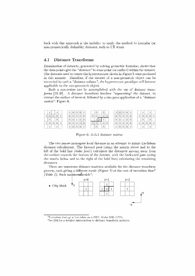
Such a conversion can be accomplished with the use of distance trans-

forms [13{23]. A distance transform involves "segmenting" the dataset, to

extract the surface of interest, followed by a two pass application of a "distance

matrix", Figure 6.

3

225

5 5

5

2

22

2

6

6

6

6 6

6

6

65

5 5

5

3 3

33

6

6

65

5

5

5

6

6 5 6

5

656

5 1

3 3

3 3

3

6 5 6

6326

5 2 2 5

63236

6 5 6

5 5

5225

1

1

3 3

1

3 3

3 3

3 3

33

3 3

0

1

1

3

3

3 3

3

3

3

Figure 6: 5x5x5 distance matrix.

The two passes propagate local distance in an attempt to mimic Euclidean

distance calculations. The forward pass (using the matrix above and to the

left of the bold line (italic font)) calculates the distances moving away from

the surface towards the bottom of the dataset, with the backward pass (using

the matrix below and to the right of the bold line) calculating the remaining

distances.

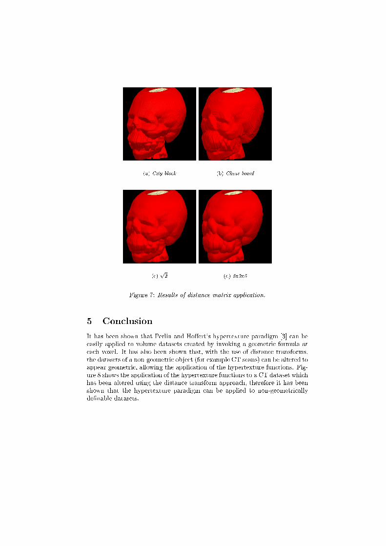
There are numerous distance matrices available for the distance transform

process, each giving a di�erent result (Figure 7) at the cost of execution time2

(Table 1). Such matrices inculde3:

� City block.

z=0 z=1 z=2

x

y

-x

-y1

1

1

1

0 11

2Execution timings where taken on a DEC Alpha 2100 4/275.3See [14] for a detailed introduction to distance transform matrices.

� Chess board.

-y

x

z=0 z=1 z=2y

-x

1

111

1

1

1

1

1

1

111

1

111

01

�p2.

-y

z=0 z=1 z=2

x

y

-x

22

22

2 2

2

11 1

1

1

01

2

2 2

2

2

Distance Average execution Average time to render

matrix time /s a 300�300 image /s

City Block 10.016 141.211

Chess Board 26.266 163.493p2 28.166 161.577

5x5x5 226.408 142.244

Table 1: Comparison of distance transform execution times.

4.2 Results

Figure 8 shows the results gained from the application of the hypertextures of

Figure 5 to a 256� 256� 113 CT dataset4, modi�ed with the distance matrix

of Figure 6.

4.3 Animation

As mentioned in Section 3 a hypertexture is created by manipulating the surface

densities of an object with a three dimensional texture function. The use

of a three dimensional texture function allows a hypertextured object to be

rendered, from di�erent view points, without any inconsistencies in the texture.

Thus introducing frame coherency for animation. Figure 9 shows a series of

frames from such an animation.

4Obtained from the University of North Carolina, Chapel Hill.

(a) City block (b) Chess board

(c)p2 (d) 5x5x5

Figure 7: Results of distance matrix application.

5 Conclusion

It has been shown that Perlin and Ho�ert's hypertexture paradigm [3] can be

easily applied to volume datasets created by invoking a geometric formula at

each voxel. It has also been shown that, with the use of distance transforms,

the datasets of a non-geometric object (for example CT scans) can be altered to

appear geometric, allowing the application of the hypertexture functions. Fig-

ure 8 shows the application of the hypertexture functions to a CT dataset which

has been altered using the distance transform approach, therefore it has been

shown that the hypertexture paradigm can be applied to non-geometrically

de�nable datasets.

(a) Bump (b) Melting (c) Low frequency �re

(d) High frequency �re (e) Fur (f) Longer fur

Figure 8: Extended hypertextures.

References

[1] J. D. Foley, A. van Dam, S. K. Feiner, and J. F. Hughes. Computer

Graphics Principles and Practice. Addison-Wesley, second edition, 1990.

[2] A. Watt and M. Watt. Advanced Animation and Rendering Techniquies

Theory and Practice. Addison-Wesley, 1992.

[3] K. Perlin and E. Ho�ert. Hypertexture. In Computer Graphics (SIG-

GRAPH '89 Proceedings), volume 23(3), pages 253{262, Boston, Mas-

sachusetts, 31 July{4 August 1989.

[4] B. Schachter. Long crested wave models. Computer Graphics and Image

Processing, 12:187{201, 1980.

[5] D. R. Peachey. Solid texturing of complex surfaces. In Computer Graphics

(SIGGRAPH '85 Proceedings), volume 19(3), pages 279{286, San Fran-

cisco, California, 22{26 July 1985.

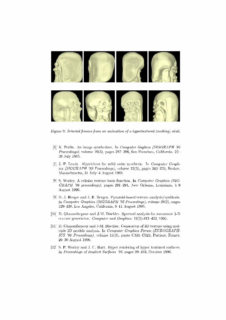
Figure 9: Selected frames from an animation of a hypertextured (melting) skull.

[6] K. Perlin. An image synthesizer. In Computer Gaphics (SIGGRAPH '85

Proceedings), volume 19(3), pages 287{296, San Francisco, California, 22{

26 July 1985.

[7] J. P. Lewis. Algorithms for solid noise synthesis. In Computer Graph-

ics (SIGGRAPH '89 Proceedings), volume 23(3), pages 263{270, Boston,

Massachusetts, 31 July{4 August 1989.

[8] S. Worley. A cellular texture basis function. In Computer Graphics (SIG-

GRAPH '96 proceedings), pages 291{294, New Orleans, Louisiana, 4{9

August 1996.

[9] D. J. Heeger and J. R. Bergen. Pyramid-based texture analysis/synthesis.

In Computer Graphics (SIGGRAPH '95 Proceedings), volume 29(2), pages

229{238, Los Angeles, California, 6{11 August 1995.

[10] D. Ghazanfarpour and J-M. Dischler. Spectral analysis for automatic 3-D

texture generation. Computer and Graphics, 19(3):413{422, 1995.

[11] D. Ghazanfarpour and J-M. Dischler. Generation of 3D texture using mul-

tiple 2D models analysis. In Computer Graphics Forum (EUROGRAPH-

ICS '96 Proceedings), volume 15(3), pages C331{C323, Poitiers, France,

26{30 August 1996.

[12] S. P. Worley and J. C. Hart. Hyper-rendering of hyper-textured surfaces.

In Proceedings of Implicit Surfaces '96, pages 99{104, October 1996.

[13] P-E. Danielsson. Euclidean distance mapping. Computer Graphics and

Image Processing, 14:227{248, 1980.

[14] G. Borgefors. Distance transformations in digital images. Computer Vi-

sion, Graphics, and Image Processing, 34(3):344{371, 1986.

[15] D. W. Paglieroni. Distance transforms: Properties and machine vision

applications. CVGIP: Graphical Models and Image Processing, 54(1):56{

74, January 1992.

[16] B. A. Payne and A. W. Toga. Distance �eld manipulation of surface

models. IEEE Computer Graphics and Applications, 12(1):65{71, 1992.

[17] G. T. Herman, J. Zheng, and C. A. Bucholtz. Shape-based interpolation.

IEEE Computer Graphics and Applications, 12(3):69{79, May 1992.

[18] I. Ragnemalm. Neighbourhoods for distance transformations using ordered

propagation. CVGIP: Image Understanding, 56(3):933{409, November

1992.

[19] R. Yagel and Z. Shi. Accelerating volume animation by space-leaping. In

Proceedings of IEEE Visualization '93, pages 62{69, October 1993.

[20] D. Cohen and Z. She�er. Proximity clouds - an acceleration technique for

3D grid traversal. The Visual Computer, 11:27{38, 1994.

[21] H. Breu, J. Gill, D. Kirkpatrick, and M. Werman. Linear time euclidean

distance transform algorithms. IEEE Transactions on Pattern Analysis

and Machine Intelligence, 17(5):529{533, May 1995.

[22] S. K. Semwal and H. Kvarnstrom. Directed safe zones and the dual ex-

tent algorithms for eÆcient grid traversal during ray tracing. In Graphics

Interface '97, pages 76{87, Kelowna, British Columbia, May 1997.

[23] D. Cohen-Or, D. Levin, and A. Solomovici. Three-dimensional distance

�eld metamorphosis. ACM Transactions on Graphics, 17(2):116{141, April

1998.