Experimental and modeling analysis of fast ionization wave dischargepropagation in a rectangular geometryKeisuke Takashima, Igor V. Adamovich, Zhongmin Xiong, Mark J. Kushner, Svetlana Starikovskaia et al. Citation: Phys. Plasmas 18, 083505 (2011); doi: 10.1063/1.3619810 View online: http://dx.doi.org/10.1063/1.3619810 View Table of Contents: http://pop.aip.org/resource/1/PHPAEN/v18/i8 Published by the AIP Publishing LLC. Additional information on Phys. PlasmasJournal Homepage: http://pop.aip.org/ Journal Information: http://pop.aip.org/about/about_the_journal Top downloads: http://pop.aip.org/features/most_downloaded Information for Authors: http://pop.aip.org/authors

Downloaded 28 Jun 2013 to 141.211.173.82. This article is copyrighted as indicated in the abstract. Reuse of AIP content is subject to the terms at: http://pop.aip.org/about/rights_and_permissions

Experimental and modeling analysis of fast ionization wave dischargepropagation in a rectangular geometry

Keisuke Takashima,1 Igor V. Adamovich,1 Zhongmin Xiong,2 Mark J. Kushner,2

Svetlana Starikovskaia,3 Uwe Czarnetzki,4 and Dirk Luggenholscher4

1Department of Mechanical and Aerospace Engineering, The Ohio State University, Columbus, Ohio 43210,USA2Department of Electrical Engineering, University of Michigan, Ann Arbor, Michigan 48109, USA3Ecole Polytechnique, Paris, France4Department of Physics and Astronomy, Ruhr University Bochum, Bochum, Germany

(Received 28 April 2011; accepted 22 June 2011; published online 17 August 2011)

Fast ionization wave (FIW), nanosecond pulse discharge propagation in nitrogen and helium in a

rectangular geometry channel=waveguide is studied experimentally using calibrated capacitive

probe measurements. The repetitive nanosecond pulse discharge in the channel was generated

using a custom designed pulsed plasma generator (peak voltage 10–40 kV, pulse duration 30–100

ns, and voltage rise time �1 kV=ns), generating a sequence of alternating polarity high-voltage

pulses at a pulse repetition rate of 20 Hz. Both negative polarity and positive polarity ionization

waves have been studied. Ionization wave speed, as well as time-resolved potential distributions

and axial electric field distributions in the propagating discharge are inferred from the capacitive

probe data. ICCD images show that at the present conditions the FIW discharge in helium is

diffuse and volume-filling, while in nitrogen the discharge propagates along the walls of the

channel. FIW discharge propagation has been analyzed numerically using quasi-one-dimensional

and two-dimensional kinetic models in a hydrodynamic (drift-diffusion), local ionization

approximation. The wave speed and the electric field distribution in the wave front predicted by the

model are in good agreement with the experimental results. A self-similar analytic solution of the

fast ionization wave propagation equations has also been obtained. The analytic model of the FIW

discharge predicts key ionization wave parameters, such as wave speed, peak electric field in the

front, potential difference across the wave, and electron density as functions of the waveform on

the high voltage electrode, in good agreement with the numerical calculations and the experimental

results. VC 2011 American Institute of Physics. [doi:10.1063/1.3619810]

I. INTRODUCTION

Over the last three decades, fast ionization wave (FIW)

discharges have been extensively studied, both experimen-

tally and theoretically. An overview of experimental results

and theoretical models published before mid-1990s is given

in review by Vasilyak et al.1 More recently, a significant

amount of experimental data on FIW dynamics and structure

has been obtained at Moscow Institute of Physics and Tech-

nology in 1994–2008,2–8 in studies of fundamental kinetic

processes in nanosecond pulse discharges and their applica-

tions. At the present time, there exists an extensive body of

data on fast ionization wave speed and attenuation coeffi-

cient in various gases in a wide range of pressures and peak

voltages, on wave front dynamics and mechanisms of its for-

mation, and on generation of high-energy (runaway) elec-

trons in the wave front. Recent experimental results also

include sub-nanosecond wave front imaging,5 visible=UV

emission spectra of FIW discharges,6,7 and inference of elec-

tric field and electron density distributions in the wave front

from calibrated capacitive probe measurements.2

The main difference between streamer discharges9–12 and

FIW discharges is that the latter demonstrate high spatial uni-

formity and reproducibility, thus allowing accurate measure-

ments of discharge parameters in a repetitively pulsed mode.

Similarity between these two types of discharges is due to the

fact that key elementary processes controlling discharge propa-

gation are electron impact ionization in the discharge front and

photoionization. Due to the high reduced electric field in the

discharge front,13 the role of high-energy electrons in ionization

kinetics can be significant.14,15 The transition between the

streamer and the ionization wave mode is rather gradual. Thus,

reducing the pressure while keeping the high voltage pulse

waveform fixed increases the streamer diameter,12 and at suffi-

ciently low pressures in a large-volume chamber the discharge

transforms into a spherical wave propagating from the high-

voltage electrode.16 Previously, development and propagation

of FIW discharges in long tubes (at the conditions when the

electrode gap is much greater compared to the discharge tube

diameter) have been studied at low pressures (1–10 Torr), at

peak pulse voltages of 10–20 kV, and at relatively high pres-

sures (up to 1 bar), at pulse voltages of 100–200 kV. In both

cases, pulse voltage rise rate was of the order of 1 kV=ns or

higher, and pulse duration was within a few tens of nanosec-

onds. It has been shown that at these conditions, the discharge

always initiates near the high-voltage electrode, with the cur-

rent loop closed by the displacement current, with the wave

speed (determined from time-resolved measurements of electri-

cal potential distributions and optical emission in the wave

front) is in the range of 1–10 cm=ns. The dependence of the

1070-664X/2011/18(8)/083505/17/$30.00 VC 2011 American Institute of Physics18, 083505-1

PHYSICS OF PLASMAS 18, 083505 (2011)

Downloaded 28 Jun 2013 to 141.211.173.82. This article is copyrighted as indicated in the abstract. Reuse of AIP content is subject to the terms at: http://pop.aip.org/about/rights_and_permissions

wave speed on pressure and discharge tube diameter is dis-

cussed in Ref. 17.

Current interest in characterization of FIW discharges is

driven mainly by their potential for applications such as

plasma chemical fuel reforming, plasma-assisted combustion,

high-speed flow control, pumping of electric discharge excited

lasers, and generation of high-energy electrons. A unique

capability of FIW discharges to generate significant ionization

and high concentrations of excited species at high pressures

and over large distances, before ionization instabilities have

time to develop, is very attractive for these applications.

Recent advances in laser optical diagnostics, such as Thomson

scattering, nanosecond and picosecond coherent anti-stokes

Raman spectroscopy, laser induced fluorescence, and laser

collision induced fluorescence are finally making possible

detailed, non-intrusive, spatially and time-resolved measure-

ments of electron density and electric field distributions in

high-speed ionization wave discharges, on nanosecond time

scale. Insight into FIW formation and propagation dynamics

also requires development of predictive kinetic models, and

their validation by the new experimental results. Note that

although numerical kinetic models may incorporate detailed

kinetics of charged and neutral species in the propagating ioni-

zation wave front (including non-local electron kinetics), ana-

lytic models remain attractive due to their capability of

elucidating fundamental trends of discharge development.

The main objectives of the present work are (i) develop-

ment and testing of the experimental apparatus for studies of

FIW discharges which lends itself to the use of advanced op-

tical diagnostics, (ii) measurements of FIW speed and elec-

tric field in the wave front by a calibrated capacitive probe,

(iii) comparison of the experimental results with kinetic

modeling calculations, and (iv) development of a predictive

analytic model of FIW propagation.

II. EXPERIMENTAL

The schematic of the experimental apparatus for studies of

fast ionization wave discharge propagation is shown in Fig. 1.

The ionization wave is generated in a rectangular cross section

quartz channel, between a high voltage electrode on the left

and a grounded electrode on the right. The high voltage elec-

trode is a 12 mm outside diameter, 10 mm inside diameter hol-

low cylinder of 32.5 mm long, with a 10 mm thick circular

base and 45 mm in diameter, made of copper. The grounded

electrode is a 16 mm thick, 100 mm� 100 mm square copper

flange, with a circular port 25 mm in diameter. The 22

mm� 13.5 mm outside dimension rectangular cross section,

20 cm long quartz channel with 1.75 mm thick walls is fused

to two quartz tube sections 14 cm long and 25 mm in diameter

on both ends, as shown in Fig. 1. The grounded flange is con-

nected to two copper waveguide plates 76 mm wide, mounted

above and below the quartz channel, as shown in Fig. 1. The

distance between the waveguide plates can be adjusted. In the

present experiments, the waveguide plates are set 40 mm apart.

The distance between the edges of the high voltage electrode

to the grounded electrode is 28 cm. The high voltage electrode

is placed between two Teflon flanges, as shown in Fig. 1, and

is connected to a high voltage terminal of a custom-designed,

high-voltage, nanosecond pulse generator. The grounded termi-

nal of the pulse generator is connected to the waveguide plates,

thus forming a plane geometry plasma waveguide. Both the

Teflon flanges and the grounded copper flange are mounted on

a base plate made of glass fiber-reinforced plastic.

In the present experiments, a capacitive probe has been

used to detect the arrival of ionization wave generated when a

voltage pulse is applied to the high voltage electrode and trav-

eling along the waveguide. This technique has been exten-

sively used previously for FIW discharge diagnostics.2–4

The capacitive probe is mounted in a 5 mm wide slot

machined in the top waveguide plate and tightened with set

screws, with the probe tip extending into the waveguide

through the slot. The probe can slide along the discharge

channel, between the leftmost and the rightmost positions,

x¼ 5 cm and x¼ 25 cm from the edge of the high voltage

electrode. Details of the probe operation and its use for the

surface charge, electric potential, and electric field distribu-

tion measurements in nanosecond pulse discharges are dis-

cussed in Ref. 2. The design of the probe used in the present

experiments is described in greater detail in our recent publi-

cation.18 Basically, the probe is a custom-made capacitive

voltage divider which consists of a coaxial feed-through ca-

pacitor (110 pF) and stray capacitance of the plasma, con-

nected to a Tektronix 3054B oscilloscope through a 50 Xterminator. The probe has a rectangular flat tip 3 mm� 12

mm, placed horizontally 8 mm above the top wall of the dis-

charge channel. During the ionization wave propagation

along the discharge channel, the probe operates as a

FIG. 1. (Color online) Schematic of the fast ionization wave discharge apparatus.

083505-2 Takashima et al. Phys. Plasmas 18, 083505 (2011)

Downloaded 28 Jun 2013 to 141.211.173.82. This article is copyrighted as indicated in the abstract. Reuse of AIP content is subject to the terms at: http://pop.aip.org/about/rights_and_permissions

capacitive voltage divider, together with a stray capacitance

between the charged wall of the channel and the plasma

formed by the ionization wave front. Basically, the probe

detects surface charge buildup on the top wall of the channel.

If the amplitude and the time response of the probe are

known, time-resolved electric potential on the discharge

channel wall at the location of the probe tip can be inferred

from the probe signal. In the present work, time response

and amplitude response of the probe are determined by cali-

bration, as discussed in Sec. III.

Optical access to the discharge channel, for discharge

imaging and emission measurements, is available from the

sides (see Fig. 1). Additional optical access is provided from

the ends of the discharge channel, through the quartz win-

dows fused to the ends of 25 mm diameter quartz endpieces

at a Brewster angle and a hollow cylinder high-voltage elec-

trode, as shown in Fig. 1. The endpieces are connected to 25

mm diameter, 25 cm long gas flow inlet and exhaust tubes,

made of glass (see Fig. 1). The main purpose of this design

is to have no grounded or floating metal parts close to the

high voltage electrode, to preclude nanosecond pulse dis-

charge propagation toward them. The present experiments

have been conducted in nitrogen and in helium at pressures

of P¼ 10–20 Torr. The baseline helium flow rate is 1 slm,

which corresponds to the flow velocity through the discharge

channel of approximately u¼ 7 m=s at P¼ 10 Torr. The

baseline nitrogen flow rate is 100 sccm (u¼ 0.7 m=s at

P¼ 10 Torr). The flow rate through the discharge section

and the pressure are controlled by mass flow controllers and

by a shutoff valve between the test section and the vacuum

pump.

The high-voltage nanosecond pulse generator used in

the present experiments has been custom designed to gener-

ate alternating polarity pulses with peak voltage of 10–30

kV, pulse duration of 30–60 ns, and pulse repetition rate up

to 50 kHz. In the present work, the pulser is operated at low

repetition rates of 10–20 Hz. The high-voltage pulses are

generated using magnetic pulse compression. The pulse out-

put voltage is regulated by varying the voltage of a DC

power supply (Heinzinger HN 1200–01, 0–1200 V, 0–100

mA) providing input to the pulse generator, UDC¼ 500–800

V. Increasing input DC voltage also reduces the output pulse

duration. Figure 2 shows typical positive and negative polar-

ity pulse shapes generated in nitrogen at P¼ 10 Torr and

�¼ 10 Hz. The experimental voltage waveforms shown in

Fig. 2 can be approximated by a Gaussian shape pulse,

U ¼ Upeak exp � t0 � t

s

� �2� �

; (1)

with s¼ 45 ns, 38 ns, 30 ns, and 26 ns for UDC¼ 560 V,

640 V, 720 V, and 800 V, respectively (full width half max-

imum (FWHM) of 75 ns, 63 ns, 50 ns, and 44 ns). The

high-voltage pulser also produces a trigger output pulse,

generated 400 ns before the main high-voltage pulse, for

synchronization with optical diagnostics. The jitter of the

trigger pulse relative to the main pulse is low, about 1 ns

for positive polarity pulses and less than 2 ns for negative

polarity pulses.

III. KINETIC MODELS

To model the ionization wave propagation in the rectangu-

lar geometry channel, shown schematically in Fig. 3 in a sim-

plified quasi-two-dimensional geometry, we used a two-fluid

hydrodynamic plasma model in the drift-diffusion approxima-

tion. In Fig. 3, the channel length and half-height are L¼ 30

cm and a¼ 0.5 cm, respectively, the dielectric thickness is

h¼ 1.5 cm, and the dielectric constant is e¼ 1. The governing

equations in the discharge channel are as follows:

@nþ@tþ div~jþ

e¼ �ine � b nþne;

~jþe¼ �Dþrnþ þ lþnþ~E;

(2)

@ne

@tþ div~je

e¼ �ine�bnþne;

~jee¼�Derne�lene

~E; (3)

Du ¼ � e

e0

nþ � neð Þ; ~E ¼ �ru; (4)

where r ¼�@=@x;

@=@y

�;D ¼ r2. The potential distribution

in the dielectric surrounding the plasma (see Fig. 3) is

FIG. 2. (Color online) Typical positive and negative polarity voltage pulse

waveforms generated by the pulsed plasma generator for different input DC

voltages.

FIG. 3. (Color online) Schematic of the plasma channel and the dielectric

layer in simplified quasi-two-dimensional geometry.

083505-3 Experimental and modeling analysis of fast ionization wave discharge propagation Phys. Plasmas 18, 083505 (2011)

Downloaded 28 Jun 2013 to 141.211.173.82. This article is copyrighted as indicated in the abstract. Reuse of AIP content is subject to the terms at: http://pop.aip.org/about/rights_and_permissions

determined from the Laplace equation, Du ¼ 0. Boundary

conditions on the positive polarity high-voltage electrode

and on the grounded electrode are as follows:

niðx ¼ 0Þ ¼ 0 @ne=@xðx ¼ 0Þ ¼ 0

neðx ¼ LÞ ¼ 0 @ni=@xðx ¼ LÞ ¼ 0; (5)

uðx ¼ 0; tÞ ¼ UðtÞ uðx ¼ L; tÞ ¼ 0: (6)

Initial conditions for the electron and ion densities and for

the potential in the discharge channel are

ne ¼ nþ ¼ no ; u ¼ 0: (7)

The surface charge density on the dielectric wall is

rw ¼ eo eEþrw � E�rw

� �; (8)

where Eþyw and E�yw are transverse electric fields on the wall

(i.e., at y¼ a, see Fig. 3), on the plasma side and on the

dielectric side, respectively.

Following the method developed by Lagarkov and Rut-

kevich,19 i.e., integrating Eqs. (2)–(4) over the transverse

coordinate (y), while assuming that the potential distribution

has the same y-dependence as in a linear electrostatic wave

and that transverse nonuniformity of the ionization wave is

weak, Eqs. (2)–(4) can be reduced to a system with only one

(axial) coordinate x,

@nþ@tþ div~jþx

e¼ �ine � b nþne; (20)

@ne

@tþ div~jex

e� lenek2u ¼ �ine � bnþne; (30)

@Ex

@xþ k2u ¼ e

e0

q; Ex ¼ �@u@x

: (40)

In Eqs. (20)–(40), k is the wavenumber of a linear electrostatic

wave formed in a weakly pre-ionized, rectangular geometry

waveguide (see Fig. 3) at the conditions when ionization is

negligible,19

tanðkaÞ tanðkhÞ ¼ v ¼ e

1þ re0f

¼ e

1þ eneleE

e0f

;

f ¼ 1

ududt; E � Ex: (9)

For small wavenumbers (i.e., long wavelengths), a simple as-

ymptotic expression for the wavenumber is valid,

ka << 1; kh << 1 : k � vah

� �1=2

: (10)

In the present work, we assume that the rate of electron

impact ionization is controlled by the local electric field.

The expression for the ionization frequency, �i, used in Eqs.

(20)–(40) is a fit to the experimental data on Townsend ioniza-

tion coefficient in nitrogen and helium as a function of the

reduced electric field, E=p,20

ap

� N2

¼

900

E=p� exp � 315

E=p

� �cm�1 ;

E

p< 100 V=cm � Torr

12 � exp � 342

E=p

� �cm�1 ; 100 <

E

p< 800 V=cm � Torr

8>>><>>>:

�i ¼ aleE:

ap

� He

¼ 3 � exp � 34

E=p

� �cm�1 ; 20 <

E

p< 150 V=cm � Torr

(11)

This problem formulation also does not incorporate photo-

ionization and ionization in collisions of excited species. A

constant electron mobility, lep¼ 0.42�106 cm2�Torr=V�s for

N2 and lep¼ 0.86�106 cm2�Torr=V�s for He,20 was assumed.

Since both electron-ion recombination and ion drift are

extremely slow on the time scale of wave propagation

(tens of nanoseconds), the recombination rate coefficient,

b¼ 10�8 cm3=s, and the ion mobility, lþp¼ 0.21�104

cm2�Torr=V�s, have almost no effect on the results. Simi-

larly, both electron diffusion and ion diffusion are com-

pletely negligible on this time scale. The initial electron

density is taken to be n0¼ 107 cm�3. In the present 1-D sim-

ulations, a uniform mesh with 5000 points has been used,

with the spatial resolution of �0.1 mm, much smaller com-

pared to the ionization wave front=space charge region thick-

ness, �5 mm (see discussion in Sec. IV B below).

Calculations using 2500 mesh points produced nearly identi-

cal results.

In addition to 1-D simulations, two-dimensional simula-

tions were performed with nonPDPSIM (NON-structured

Plasma Display Panel SIMulation) a 2-D plasma hydrody-

namics model with radiation photon transport. In non-PDPSIM, continuity equations for charged and neutral

species, and Poisson’s equation for electric potential are inte-

grated coincidently in time with the electron energy equa-

tion, with transport coefficients obtained from stationary

solutions of the Boltzmann equation. The use of the electron

energy equation allows for non-equilibrium between the

local electric field and electron transport coefficients. The

spatial discretization in nonPDPSIM is based on a finite vol-

ume method on an unstructured mesh. The time integration

of Poisson’s equation and charged particle transport are

083505-4 Takashima et al. Phys. Plasmas 18, 083505 (2011)

Downloaded 28 Jun 2013 to 141.211.173.82. This article is copyrighted as indicated in the abstract. Reuse of AIP content is subject to the terms at: http://pop.aip.org/about/rights_and_permissions

implemented with a fully implicit Newton iteration method.

The transport of photon radiation is addressed using a propa-

gator—Green’s function method. The details of the model

and the solution method are described in Refs. 21 and 22.

The 2-D geometry used in the model is based on the experi-

mental setup described above, shown in Fig. 1, including the

powered and the grounded electrodes, the metal waveguide, and

the dielectric discharge channel filled with nitrogen with a small

amount of oxygen (N2=O2¼ 99.9%=0.1%) at 10 Torr and 300

K. Adding a small amount of O2 does not significantly affect the

FIW dynamics but does provide a mechanism for photo-ioniza-

tion which, for a positive polarity discharge, is required to pro-

vide seed electrons ahead of the ionization front. The discharge

is assumed to be symmetric about the channel center line. The

initial electron density in the channel is assumed to be zero,

except for a small spot of plasma (0.5 cm in diameter, maximum

electron density of 1010 cm�3) near the tip of the powered elec-

trode. This seeding is required to initiate the plasma in the ab-

sence of electric field emission from the positively biased

electrode. A nonzero electron density ahead of the ionization

front, necessary for the propagation of the ionization front in the

positive polarity case, is produced through photoionization of O2

additive by the UV photon flux from radiating nitrogen species

N2(C3Pu), generated behind the ionization front.

In the present 2-D simulation, an unstructured mesh

with a total of 9300 grid points is used. The mesh in the

plasma region is refined such that there are about 15 grid

points cross the ionization front (with thickness in the axial

direction of about 1 cm, see discussion in Sec. IV B below).

A simulation with doubled grid resolution was also per-

formed, and the distributions of the electron density, axial

electric field, and ionization source function at the ionization

front are found to be nearly identical.

Both in the 1-D and in the 2-D modeling calculations,

the experimental pulse voltage waveforms were approxi-

mated by a Gaussian shape pulse, given by Eq. (1).

IV. RESULTS AND DISCUSSION

A. Wave speed and electric field measurements

In the present work, the capacitive probe was calibrated

using the following procedure. First, the time response of the

probe was determined by placing the probe tip next to a

coaxial cable transmitting a rectangular shape voltage pulse

(peak voltage 4 V, 50 ns pulse duration, 8 ns rise time, 7 ns

fall time) produced by a SRS DG535 delay generator. To

detect the pulse, part of the cable coaxial shielding was

removed. The response time of the probe, s¼ 8 ns, was

found from the following equation,18

UðtÞ ¼ A VðtÞ þ 1

s

ðt

0

Vðt0Þdt0� �

; (12)

where U(t) is the voltage pulse shape in the cable and V(t) is

probe signal. The amplitude response of the probe, A, was

measured by placing a rectangular cross section shell made

of copper foil inside the quartz discharge channel, with the

foil following closely the channel walls. The shell was con-

nected to the high-voltage electrode, powered by the high-

voltage nanosecond pulse generator, and extended along

most of the channel. Thus, a high-voltage pulse U(t) of

known amplitude and shape, measured on the electrode by a

Tektronix P6015A high voltage probe, was applied to the

entire shell. The amplitude response of the capacitive probe,

with the tip located 8 mm above the quartz channel, was

again obtained from Eq. (12), A¼ 5.0�103. Finally, the spatial

response of the probe was determined by translating it along

the channel and measuring the pulse potential at different dis-

tances from the end of the copper foil shell serving as a high

voltage electrode extension, at the conditions when no break-

down is produced in the channel. In the absence of volume

ionization, the potential distribution in the channel is a linear

electrostatic wave, u¼ const at x< 0 and u(x,t)�exp(-kx-ift)at x� 0, where x is the axial distance from the end of the

shell, with the wavenumber for the plane geometry with air

dielectric given by Eq. (9), tan(ka)tan(kh) � 1. For a¼ 0.5

cm and h¼ 1.5 cm, this gives k¼ 0.79 cm�1. The asymptotic

pulse peak potential distribution at x� 0, measured during

probe calibration, follows the exponential decay curve,

/(x)¼ exp(-kx), with the wave number close to the value pre-

dicted by theory, k¼ 0.65 cm�1. The calibration data, /(x),

are well reproduced by using the Gaussian probe spatial

response function, gðxÞ ¼ exp½�ðx�x0

d Þ2�, with d¼ 13 6 2

mm, such that /ðx0Þ ¼Ðþ1�1 uðxÞgðx� x0Þdx. This corre-

sponds to the FWHM probe response of DFWHM � 22 6 3

mm. After calibration, the height and the orientation of the

probe tip were kept the same. As discussed in Sec. II, for

measurements at different locations the probe was translated

along the discharge channel by sliding along the slot

machined in the top waveguide plate.

Figure 4(a) plots raw capacitive probe signals measured

in helium, at P¼ 20 Torr, �¼ 20 Hz, and UDC¼V, for a pos-

itive polarity wave (pulse peak voltage þ10.5 kV). The

probe signals are taken for multiple probe tip locations rang-

ing from x¼ 5 cm to x¼ 25 cm from the high voltage elec-

trode, 1 cm apart. The traces in Fig. 4(a) are averaged over

200 positive polarity discharge pulses (i.e., 20 s). It can be

seen that the results are reproduced very well run-to-run,

with excellent signal-to-noise. Note that this is critical for in-

ference of the electric field from the probe signals. The high-

voltage pulse waveform is also shown in Fig. 4(a), on the

same time scale. Figure 4(b) plots electric potentials at these

probe locations, u(t), inferred from the raw probe signals,

V(t), using Eq. (12). The potentials in Fig. 4(b) are also plot-

ted together with the high-voltage pulse (i.e., the potential on

the high-voltage electrode, U(t)). Figure 4(b) illustrates that

the wave of electric potential propagates to the right, from

the high voltage electrode to the grounded electrode. The

potentials measured by the probe start decreasing when the

wave reaches the grounded electrode, which occurs approxi-

mately at t¼ 72 ns. Figure 4(c) plots time-resolved axial

electric field at midpoints between the probe locations, i.e.,

at x¼ 5.5, 6.5,…,24.5 cm, determined from the potential dif-

ference at these locations. It can be seen that the wave front

initially steepens while peak electric field increases consider-

ably (from less than 1 kV=cm to more than 2 kV=cm), before

reaching a quasi-steady-state shape (at x � 14 cm), when

083505-5 Experimental and modeling analysis of fast ionization wave discharge propagation Phys. Plasmas 18, 083505 (2011)

Downloaded 28 Jun 2013 to 141.211.173.82. This article is copyrighted as indicated in the abstract. Reuse of AIP content is subject to the terms at: http://pop.aip.org/about/rights_and_permissions

peak electric field in the front starts gradually decreasing.

Finally, Figure 4(d) plots the wave front location, as well as

peak electric field and potential at the moment when the field

peaks, vs. time. The uncertainty of the capacitive probe tip

location is 60.5 mm, and the estimated uncertainty of the

wave speed inferred from the slope of the x-t diagram such

as shown in Fig. 4(d) is 2%. From Fig. 4(d), it can be seen

that far from the high voltage electrode (at x> 11 cm), the

wave speed becomes nearly constant, V¼ 0.32 cm=ns at

x¼ 11–25 cm. In this region, peak electric field in the wave

front and the potential at the location of the peak field are

gradually decaying, E � 2.0–1.8 kV=cm and U¼ 5.0–4.0

kV, respectively.

Figures 5 and 6 plot time-resolved electric field and the

wave trajectory, along with peak electric fields and corre-

sponding potentials, for positive and negative polarity waves

in nitrogen, at P¼ 10 Torr, �¼Hz, and UDC¼ 640 V (pulse

peak voltages þ20 and �21 kV, respectively). It can be seen

that the negative polarity wave is more spread out, with peak

electric field in the wave front not exceeding E¼ 3 kV=cm

(compared to approximately E¼ 4 kV=cm in the positive po-

larity wave). In both cases, the wave initially steepens before

FIG. 4. (Color online) (a) Raw capacitive probe data plotted together with the high voltage pulse waveform; (b) time-resolved potentials; (c) time-resolved

axial electric fields; (d) ionization wave front location vs. time, peak electric field, and potential across the wave front at different probe locations. Data

obtained for 21 different locations of the capacitive probe 1 cm apart, ranging from 5 cm to 25 cm from the high voltage electrode. Helium, P¼ 20 Torr,

�¼ 20 Hz, U¼ 500 V, positive polarity wave (pulse peak voltage þ10.5 kV).

083505-6 Takashima et al. Phys. Plasmas 18, 083505 (2011)

Downloaded 28 Jun 2013 to 141.211.173.82. This article is copyrighted as indicated in the abstract. Reuse of AIP content is subject to the terms at: http://pop.aip.org/about/rights_and_permissions

reaching quasi-steady-state and decaying gradually. The neg-

ative polarity wave speed is significantly lower compared to

that of the positive polarity wave, V¼ 0.53 cm=ns vs.

V¼ 0.67 cm=ns (both values averaged over x¼ 10–25 cm).

The results obtained at a higher DC voltage, UDC¼ 760 V

(positive and negative pulse peak voltages of þ28.3 kV and

�29.7 kV, respectively), are similar to the ones plotted in

Figs. 5 and 6, and show similar trends. In this case, the wave

speed was significantly higher, V¼ 1.02 cm=ns for positive

polarity and V¼ 0.88 cm=ns for negative polarity (a differ-

ence of approximately 15%), averaged over x¼ 10–25 cm.

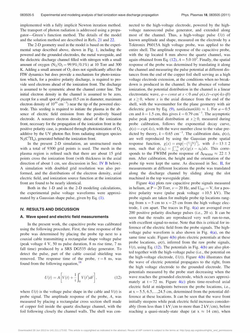
Figure 7 shows broadband, 10-shot average ICCD

(Intensified CCD or Intensified Charged Coupled Device)

camera images of positive and negative polarity ionization

waves in helium, at P¼ 20 Torr, �¼ 20 Hz, and U¼ 500 V

(pulse peak voltages þ10.5 kV and �11.0 kV). In the

images, the wave propagates left to right. The wave speed at

these conditions is V¼ 0.32 cm=ns and V¼ 0.21 cm=ns,

respectively, such that the 4 ns camera gate provides spatial

resolution of approximately 1 cm. The field of view of the

images is 4.6 cm� 3.1 cm. The camera was triggered exter-

nally, by a trigger pulse provided by the high-voltage pulse

generator. The trigger pulse jitter relative to the main high

voltage pulse is low, about 1 ns for positive polarity pulses

and less than 2 ns for negative polarity pulses. Pulse-to-pulse

reproducibility of the ionization wave launch timing and

wave speed and is so good that 10-shot images shown appear

essentially identical to the single-shot images. One can see

that emission intensity distribution from the positive polarity

wave is fairly uniform, while in the negative polarity wave

emission is brighter near the top and bottom walls of the

channel.

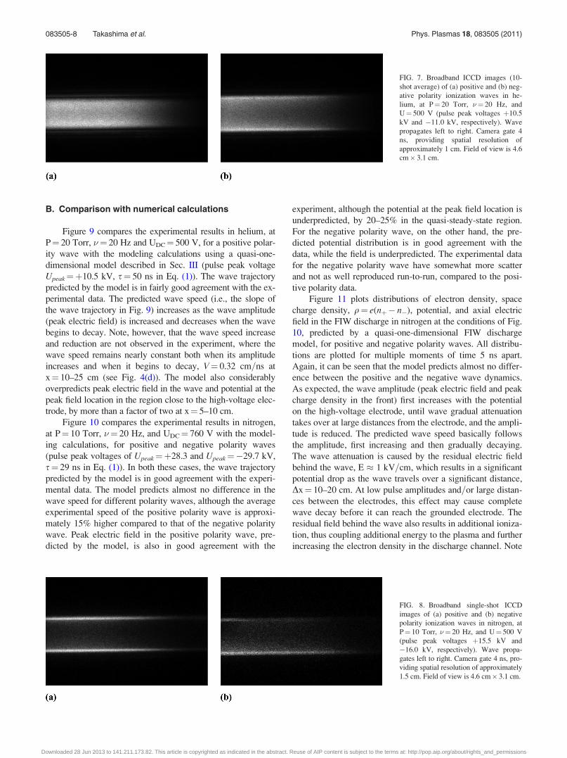
Figure 8 shows broadband single-shot ICCD images of

positive and negative polarity ionization waves in nitrogen,

at P¼ 10 Torr, �¼ 20 Hz, and UDC¼ 500 V (pulse peak vol-

tages þ15.5 kV and �16.0 kV). The wave speed at these

conditions is V¼ 0.40 cm=ns and V¼ 0.36 cm=ns, providing

spatial resolution of approximately 1.5 cm. From Figure 8, it

can be seen that the ionization wave in nitrogen propagates

mainly along the walls of the discharge channel. This is con-

sistent with the visual observation of the discharge through

the windows in the endpieces of the discharge channel (see

Fig. 1), which also shows that emission is brightest along the

perimeter of the discharge channel.

FIG. 5. (Color online) (a) Time-resolved

axial electric fields; (b) ionization wave

front location vs. time, peak electric field,

and potential across the wave front at dif-

ferent probe locations. Nitrogen, P¼ 10

Torr, �¼ 20 Hz, U¼ 640 V, positive po-

larity wave (pulse peak voltageþ20 kV).

FIG. 6. (Color online) (a) Time-resolved

axial electric fields; (b) ionization wave

front location vs. time, peak electric field,

and potential across the wave front at dif-

ferent probe locations. Nitrogen, P¼ 10

Torr, �¼ 20 Hz, U¼ 640 V, negative po-

larity wave (pulse peak voltage �21 kV).

083505-7 Experimental and modeling analysis of fast ionization wave discharge propagation Phys. Plasmas 18, 083505 (2011)

Downloaded 28 Jun 2013 to 141.211.173.82. This article is copyrighted as indicated in the abstract. Reuse of AIP content is subject to the terms at: http://pop.aip.org/about/rights_and_permissions

B. Comparison with numerical calculations

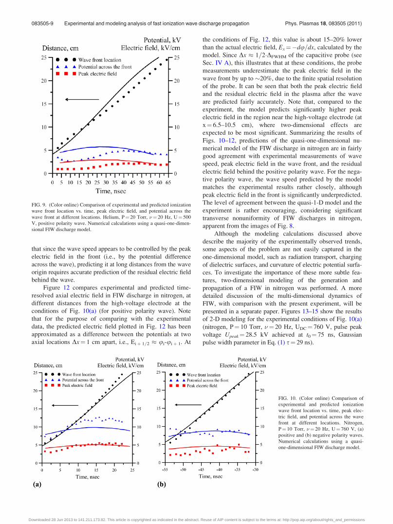
Figure 9 compares the experimental results in helium, at

P¼ 20 Torr, �¼ 20 Hz and UDC¼ 500 V, for a positive polar-

ity wave with the modeling calculations using a quasi-one-

dimensional model described in Sec. III (pulse peak voltage

Upeak¼þ10.5 kV, s¼ 50 ns in Eq. (1)). The wave trajectory

predicted by the model is in fairly good agreement with the ex-

perimental data. The predicted wave speed (i.e., the slope of

the wave trajectory in Fig. 9) increases as the wave amplitude

(peak electric field) is increased and decreases when the wave

begins to decay. Note, however, that the wave speed increase

and reduction are not observed in the experiment, where the

wave speed remains nearly constant both when its amplitude

increases and when it begins to decay, V¼ 0.32 cm=ns at

x¼ 10–25 cm (see Fig. 4(d)). The model also considerably

overpredicts peak electric field in the wave and potential at the

peak field location in the region close to the high-voltage elec-

trode, by more than a factor of two at x¼ 5–10 cm.

Figure 10 compares the experimental results in nitrogen,

at P¼ 10 Torr, �¼ 20 Hz, and UDC¼ 760 V with the model-

ing calculations, for positive and negative polarity waves

(pulse peak voltages of Upeak¼þ28.3 and Upeak¼�29.7 kV,

s¼ 29 ns in Eq. (1)). In both these cases, the wave trajectory

predicted by the model is in good agreement with the experi-

mental data. The model predicts almost no difference in the

wave speed for different polarity waves, although the average

experimental speed of the positive polarity wave is approxi-

mately 15% higher compared to that of the negative polarity

wave. Peak electric field in the positive polarity wave, pre-

dicted by the model, is also in good agreement with the

experiment, although the potential at the peak field location is

underpredicted, by 20–25% in the quasi-steady-state region.

For the negative polarity wave, on the other hand, the pre-

dicted potential distribution is in good agreement with the

data, while the field is underpredicted. The experimental data

for the negative polarity wave have somewhat more scatter

and not as well reproduced run-to-run, compared to the posi-

tive polarity data.

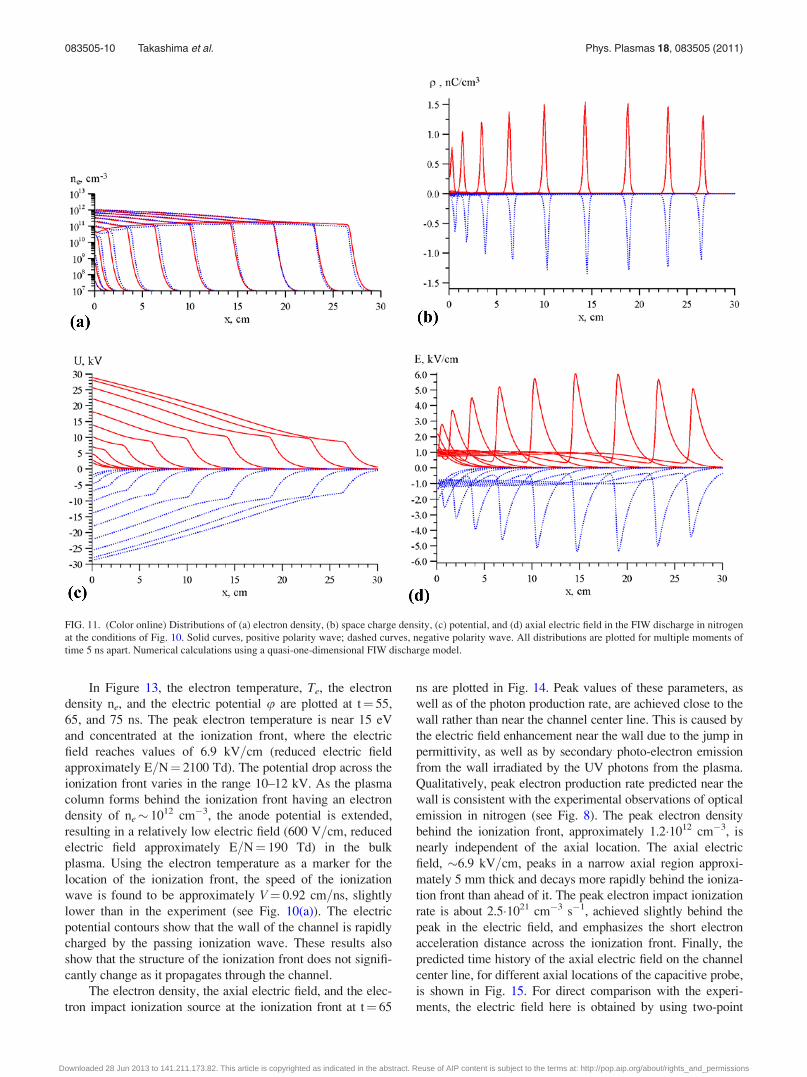
Figure 11 plots distributions of electron density, space

charge density, q¼ e(nþ� n�), potential, and axial electric

field in the FIW discharge in nitrogen at the conditions of Fig.

10, predicted by a quasi-one-dimensional FIW discharge

model, for positive and negative polarity waves. All distribu-

tions are plotted for multiple moments of time 5 ns apart.

Again, it can be seen that the model predicts almost no differ-

ence between the positive and the negative wave dynamics.

As expected, the wave amplitude (peak electric field and peak

charge density in the front) first increases with the potential

on the high-voltage electrode, until wave gradual attenuation

takes over at large distances from the electrode, and the ampli-

tude is reduced. The predicted wave speed basically follows

the amplitude, first increasing and then gradually decaying.

The wave attenuation is caused by the residual electric field

behind the wave, E � 1 kV=cm, which results in a significant

potential drop as the wave travels over a significant distance,

Dx¼ 10–20 cm. At low pulse amplitudes and=or large distan-

ces between the electrodes, this effect may cause complete

wave decay before it can reach the grounded electrode. The

residual field behind the wave also results in additional ioniza-

tion, thus coupling additional energy to the plasma and further

increasing the electron density in the discharge channel. Note

FIG. 7. Broadband ICCD images (10-

shot average) of (a) positive and (b) neg-

ative polarity ionization waves in he-

lium, at P¼ 20 Torr, �¼ 20 Hz, and

U¼ 500 V (pulse peak voltages þ10.5

kV and �11.0 kV, respectively). Wave

propagates left to right. Camera gate 4

ns, providing spatial resolution of

approximately 1 cm. Field of view is 4.6

cm� 3.1 cm.

FIG. 8. Broadband single-shot ICCD

images of (a) positive and (b) negative

polarity ionization waves in nitrogen, at

P¼ 10 Torr, �¼ 20 Hz, and U¼ 500 V

(pulse peak voltages þ15.5 kV and

�16.0 kV, respectively). Wave propa-

gates left to right. Camera gate 4 ns, pro-

viding spatial resolution of approximately

1.5 cm. Field of view is 4.6 cm� 3.1 cm.

083505-8 Takashima et al. Phys. Plasmas 18, 083505 (2011)

Downloaded 28 Jun 2013 to 141.211.173.82. This article is copyrighted as indicated in the abstract. Reuse of AIP content is subject to the terms at: http://pop.aip.org/about/rights_and_permissions

that since the wave speed appears to be controlled by the peak

electric field in the front (i.e., by the potential difference

across the wave), predicting it at long distances from the wave

origin requires accurate prediction of the residual electric field

behind the wave.

Figure 12 compares experimental and predicted time-

resolved axial electric field in FIW discharge in nitrogen, at

different distances from the high-voltage electrode at the

conditions of Fig. 10(a) (for positive polarity wave). Note

that for the purpose of comparing with the experimental

data, the predicted electric field plotted in Fig. 12 has been

approximated as a difference between the potentials at two

axial locations Dx¼ 1 cm apart, i.e., Eiþ 1=2 � ui-uiþ 1. At

the conditions of Fig. 12, this value is about 15–20% lower

than the actual electric field, Ex¼�du=dx, calculated by the

model. Since Dx � 1=2�DFWHM of the capacitive probe (see

Sec. IV A), this illustrates that at these conditions, the probe

measurements underestimate the peak electric field in the

wave front by up to �20%, due to the finite spatial resolution

of the probe. It can be seen that both the peak electric field

and the residual electric field in the plasma after the wave

are predicted fairly accurately. Note that, compared to the

experiment, the model predicts significantly higher peak

electric field in the region near the high-voltage electrode (at

x¼ 6.5–10.5 cm), where two-dimensional effects are

expected to be most significant. Summarizing the results of

Figs. 10–12, predictions of the quasi-one-dimensional nu-

merical model of the FIW discharge in nitrogen are in fairly

good agreement with experimental measurements of wave

speed, peak electric field in the wave front, and the residual

electric field behind the positive polarity wave. For the nega-

tive polarity wave, the wave speed predicted by the model

matches the experimental results rather closely, although

peak electric field in the front is significantly underpredicted.

The level of agreement between the quasi-1-D model and the

experiment is rather encouraging, considering significant

transverse nonuniformity of FIW discharges in nitrogen,

apparent from the images of Fig. 8.

Although the modeling calculations discussed above

describe the majority of the experimentally observed trends,

some aspects of the problem are not easily captured in the

one-dimensional model, such as radiation transport, charging

of dielectric surfaces, and curvature of electric potential surfa-

ces. To investigate the importance of these more subtle fea-

tures, two-dimensional modeling of the generation and

propagation of a FIW in nitrogen was performed. A more

detailed discussion of the multi-dimensional dynamics of

FIW, with comparison with the present experiment, will be

presented in a separate paper. Figures 13–15 show the results

of 2-D modeling for the experimental conditions of Fig. 10(a)

(nitrogen, P¼ 10 Torr, �¼ 20 Hz, UDC¼ 760 V, pulse peak

voltage Upeak¼ 28.5 kV achieved at t0¼ 75 ns, Gaussian

pulse width parameter in Eq. (1) s¼ 29 ns).

FIG. 10. (Color online) Comparison of

experimental and predicted ionization

wave front location vs. time, peak elec-

tric field, and potential across the wave

front at different locations. Nitrogen,

P¼ 10 Torr, �¼ 20 Hz, U¼ 760 V, (a)

positive and (b) negative polarity waves.

Numerical calculations using a quasi-

one-dimensional FIW discharge model.

FIG. 9. (Color online) Comparison of experimental and predicted ionization

wave front location vs. time, peak electric field, and potential across the

wave front at different locations. Helium, P¼ 20 Torr, �¼ 20 Hz, U¼ 500

V, positive polarity wave. Numerical calculations using a quasi-one-dimen-

sional FIW discharge model.

083505-9 Experimental and modeling analysis of fast ionization wave discharge propagation Phys. Plasmas 18, 083505 (2011)

Downloaded 28 Jun 2013 to 141.211.173.82. This article is copyrighted as indicated in the abstract. Reuse of AIP content is subject to the terms at: http://pop.aip.org/about/rights_and_permissions

In Figure 13, the electron temperature, Te, the electron

density ne, and the electric potential u are plotted at t¼ 55,

65, and 75 ns. The peak electron temperature is near 15 eV

and concentrated at the ionization front, where the electric

field reaches values of 6.9 kV=cm (reduced electric field

approximately E=N¼ 2100 Td). The potential drop across the

ionization front varies in the range 10–12 kV. As the plasma

column forms behind the ionization front having an electron

density of ne� 1012 cm�3, the anode potential is extended,

resulting in a relatively low electric field (600 V=cm, reduced

electric field approximately E=N¼ 190 Td) in the bulk

plasma. Using the electron temperature as a marker for the

location of the ionization front, the speed of the ionization

wave is found to be approximately V¼ 0.92 cm=ns, slightly

lower than in the experiment (see Fig. 10(a)). The electric

potential contours show that the wall of the channel is rapidly

charged by the passing ionization wave. These results also

show that the structure of the ionization front does not signifi-

cantly change as it propagates through the channel.

The electron density, the axial electric field, and the elec-

tron impact ionization source at the ionization front at t¼ 65

ns are plotted in Fig. 14. Peak values of these parameters, as

well as of the photon production rate, are achieved close to the

wall rather than near the channel center line. This is caused by

the electric field enhancement near the wall due to the jump in

permittivity, as well as by secondary photo-electron emission

from the wall irradiated by the UV photons from the plasma.

Qualitatively, peak electron production rate predicted near the

wall is consistent with the experimental observations of optical

emission in nitrogen (see Fig. 8). The peak electron density

behind the ionization front, approximately 1.2�1012 cm�3, is

nearly independent of the axial location. The axial electric

field, �6.9 kV=cm, peaks in a narrow axial region approxi-

mately 5 mm thick and decays more rapidly behind the ioniza-

tion front than ahead of it. The peak electron impact ionization

rate is about 2.5�1021 cm�3 s�1, achieved slightly behind the

peak in the electric field, and emphasizes the short electron

acceleration distance across the ionization front. Finally, the

predicted time history of the axial electric field on the channel

center line, for different axial locations of the capacitive probe,

is shown in Fig. 15. For direct comparison with the experi-

ments, the electric field here is obtained by using two-point

FIG. 11. (Color online) Distributions of (a) electron density, (b) space charge density, (c) potential, and (d) axial electric field in the FIW discharge in nitrogen

at the conditions of Fig. 10. Solid curves, positive polarity wave; dashed curves, negative polarity wave. All distributions are plotted for multiple moments of

time 5 ns apart. Numerical calculations using a quasi-one-dimensional FIW discharge model.

083505-10 Takashima et al. Phys. Plasmas 18, 083505 (2011)

Downloaded 28 Jun 2013 to 141.211.173.82. This article is copyrighted as indicated in the abstract. Reuse of AIP content is subject to the terms at: http://pop.aip.org/about/rights_and_permissions

potential difference, as was also done in the 1-D case (see Fig.

12). The resulting electric field is found to be 10% lower than

the instantaneous local value produced by differentiation of

the electric potential obtained from the model. The shape of

the axial electric field is quite close to the experimental meas-

urements, and the quantitative agreement at x> 12.5 cm is

rather good (compare with Fig. 12(a)). Near the powered elec-

trode (at x< 12.5 cm), the computed values are about a factor

of two higher than in experiment (see Fig. 12(a). However,

this discrepancy is somewhat expected as the details of the 3-

D, cylindrical shape powered electrode are not well captured

in the 2-D planar simulations.

C. Self-similar analytic solution for ionizationwave propagation

Following the approach19 and introducing a self-similar

spatial coordinate n¼ xþVt, where V is wave speed (such

that @=@x ¼ @=@n, @=@t ¼ V@=@n), while neglecting ion drift,

recombination, and diffusion on a short time scale, Eqs. (20)–(40) can be reduced to a system of ordinary differential equa-

tions for the electron density (n), space charge density (q),

and axial electric field (E):

dn

dn¼ �in

V þ w; (13)

dE

dn¼ k2u� e

e0

q; (14)

dqdn¼ lE�in

VðV þ wÞ �elnq

e0ðV þ wÞ : (15)

Here, w¼ lE is the electron drift velocity, such that wV.

The difference between the positive and the negative polarity

waves is that the sign of the drift velocity is changed from

plus to minus. The ionization frequency is approximated as

follows:

�i ¼ Ap exp �Bp

E

� � lE; (16)

FIG. 12. (Color online) Comparison of (a) experimental and (b) predicted

time-resolved axial electric field at different distances from the high-voltage

electrode at the conditions of Fig. 10(a) (positive polarity wave). Numerical

calculations using a quasi-one-dimensional FIW discharge model.

FIG. 13. (Color online) 2-dimensional

FIW simulation of a positive polarity

wave in nitrogen, at 10 Torr and

U¼ 760 V. (a) Electron temperature

(flood contours) and electric potential

(lines); (b) electron density (flood con-

tours) and electric potential (lines),

shown at t¼ 55, 65, and 75 ns. The spac-

ing of the potential contour lines is 2 kV.

Peak electron temperature 15 eV, peak

electron density approximately 1012

cm�3. The wave speed is approximately

0.92 cm=ns.

083505-11 Experimental and modeling analysis of fast ionization wave discharge propagation Phys. Plasmas 18, 083505 (2011)

Downloaded 28 Jun 2013 to 141.211.173.82. This article is copyrighted as indicated in the abstract. Reuse of AIP content is subject to the terms at: http://pop.aip.org/about/rights_and_permissions

where A¼ 12 1=cm�Torr and B¼ 342 V=cm�Torr for nitro-

gen (see Eq. (11)).

An approximate analytic solution of Eqs. (13)–(15) has

been derived in Ref. 19, to predict the dependence of the

ionization wave speed and amplitude (peak electric field)

on the potential drop across the wave. However, an accurate

self-similar solution for the electric field, electron density,

and space charge density distributions in the wave front and

behind the wave has not been obtained. Also, wave speed

and amplitude have not been related to the voltage pulse pa-

rameters on the electrode (such as voltage rise time). In the

present work, the self-similar solution is obtained in three

separate regions, (I) “upstream of the wave” (before break-

down), (II) in the wave front (during breakdown), and (III)

“downstream of the wave” (in the plasma shielded by space

charge in the ionization wave front). In this solution, the

wave speed, V, is assumed to be constant and is one of the

input parameters of the model. A schematic of the quasi-

one-dimensional ionization wave structure is shown in

Fig. 16. The results for key parameter values and distribu-

tions in the wave are given below.

1. Region I (linear wave before breakdown)

Peak electric field in the ionization wave front, E*,

breakdown potential, u*, and the point where breakdown

initiates, n*, are given as follows:

�i E ¼ Ap exp �Bp

E

� � lE2

¼ 2BpVk0 lnk0e0V

eln0

� ; u ¼ E

k0

; (17)

n ¼ 1

k0

lnE

k0u0

� ; g ¼ n� n: (18)

Electron density and space charge density at breakdown

point, g*, are calculated as

n ¼ k0e0V

elq ¼ lEn

V¼ k0e0E

e: (19)

In Eqs. (17)–(19), k0 is the wavenumber of a linear electro-

static wave “upstream” of breakdown point (at n< n*,

g< 0), obtained from Eq. (9) when the plasma conductivity

is very low, r e0ðdu=dtÞ=u,

tanðk0aÞ tanðk0hÞ ¼ e k0a << 1;

k0h << 1 : k0 �e

ah

� �1=2

: (20)

FIG. 14. (Color online) Contours of (a) electron density, (b) axial electric

field, and (c) ionization source rate, illustrating the structure of the ionization

front at the conditions of Fig. 13, at t¼ 65 ns.

FIG. 15. (Color online) Time history of the electric field on the channel cen-

terline predicted by the two-dimensional model, for several axial locations

of capacitive probes, at the conditions of Fig. 13.

FIG. 16. (Color online) Schematic of a quasi-one-dimensional ionization

wave structure.

083505-12 Takashima et al. Phys. Plasmas 18, 083505 (2011)

Downloaded 28 Jun 2013 to 141.211.173.82. This article is copyrighted as indicated in the abstract. Reuse of AIP content is subject to the terms at: http://pop.aip.org/about/rights_and_permissions

Electric field, potential, space charge, and electron density

distributions in Region I are found from the following

equations:

E ¼ E exp k0gð Þ; u ¼ u exp k0gð Þ;

q ¼ q exp�i gV

� ; ðg � 0Þ (21)

n ¼n0 ; g � � E

Bpk0

n exp�i gV

1þ Bpk0

Eg2

� � �; � E

Bpk0

� g � 0

8>><>>: :

(22)

2. Region II (primary breakdown wave)

Electric field, potential, electron density, and space

charge distributions in this region are calculated as follows:

E ¼ E exp � �i gV

1� exp �Bp

E

� � E

Bp

� �; (23)

u ¼ u þ 1� exp � �i gV

1� exp �Bp

E

� � E

Bp

� � �

� BpV

�i 1� exp �Bp

E

� � ; (24)

n ¼ n þ e0�i

elE

Bp1� exp

Bp

EE� E

E

� � �; (25)

q ¼

lEn

V; g � gpeak

qpeak exp � 2eln1e0V

ðg� gpeakÞ� �

; gpeak � g

8><>: ; (26)

where

gpeak ¼VBp

2�i E1

1� exp �Bp

E

� � � ; (27)

is the point where the space charge density peaks, with the

peak value of

qpeak ¼lV

Effiffiffiep n þ e0�

i

elE

Bp1� exp �Bp

E

ffiffiffiep � 1ffiffiffi

ep

� � � �:

(28)

Potential difference across the primary wave and the electron

density after the primary wave can be found as

u1 ¼ u þ BpV

�i 1� exp �Bp

E

� � ; (29)

n1 ¼k0e0V

elþ e0�

i E

elBp1� exp �Bp

E

� � �

¼ k0e0V

el1þ 2 ln

k0e0V

eln0

� 1� exp �Bp

E

� � � �: (30)

3. Region III (secondary linear wave and secondaryionization wave)

The boundary between regions II and III is found from

the following matching condition,

q ¼ k1e0E

e: (31)

The wavenumber of the secondary linear wave, k1, can be

obtained from Eq. (9) when the plasma conductivity is high,

r� e0ðdu=dtÞ=u,

k1 ¼ee0V

aheln1: (32)

This gives the minimum value of the electric field down-

stream of the primary ionization wave, Emin, and the location

of the minimum, gmin,

Emin ¼ E exp � a2ða� bÞ

� �c�

ba�b;

gmin ¼agpeak þ ln c

a� b; (33)

where

a ¼ 2eln1e0V

; b ¼ �i

V1� exp �Bp

E

� � E

Bp;

c ¼qpeake

e0k1E: (34)

At g¼ gmin, the electric field reaches minimum, E¼Emin,

since the field is shielded by the space charge in the primary

wave front, and then starts increasing again, producing the

secondary linear wave propagating over the plasma ionized

by the primary ionization wave. When the field becomes suf-

ficiently high for the ionization to begin again, the resultant

charge separation causes the field to nearly level off, and it

reaches a quasi-steady state value Emax near point gmax,

�i;max ¼ Ap exp � Bp

Emax

� � lEmax ¼ k1V; (35)

gmax ¼ gmin þ lnEmax

Emin

� 1

k1: (36)

Ionization in this secondary wave starts affecting the electric

field and the electron density distributions at the point

gmin < g0 < gmax, such as

g0 ¼ gmin þ lnE0

Emin

� 1

k1; E0 ¼ Emax 1� Emax

Bp

� : (37)

083505-13 Experimental and modeling analysis of fast ionization wave discharge propagation Phys. Plasmas 18, 083505 (2011)

Downloaded 28 Jun 2013 to 141.211.173.82. This article is copyrighted as indicated in the abstract. Reuse of AIP content is subject to the terms at: http://pop.aip.org/about/rights_and_permissions

Until this happens (i.e., at g � g0), the field and the potential

distributions both rise exponentially, while the electron den-

sity remains constant

E ¼ Emin exp k1ðg� gminÞ½ �; (38)

u ¼ u1 þEmin

k1exp k1ðg� gminÞð Þ � 1½ �; (39)

n ¼ n1: (40)

After ionization begins again (i.e., at g0 � g), the field, the

potential, and the electron density are given as

E¼ E0Emax

E0 þ Emax�E0ð Þexp �Bpk1ðg� g0ÞEmax

� ! Emax;

(41)

u ¼ u1 þE0 � Emin

k1þ Emax ðg� g0Þ þ Emax

Bpk1ln

E0

E

� �! constþ Emaxðg� g0Þ;

(42)

n ¼ n1 exp k1ðg� g0Þ½ �E0

E: (43)

At gmax � g the electron density continues to increase with

distance approximately linearly,

n ¼ n1 1þ Emax � E0

E0Emax

E0

� �BN=Emax

" #

þ n1k1ðg� gmaxÞ ¼ constþ ee0V

ahelðg� gmaxÞ:

(44)

Finally, space charge density in the entire Region III is cal-

culated as

q ¼ e0E�

eV: (45)

The value of the “residual” electric field downstream of the

wave, Emax, given by Eq. (35), along with the rate of voltage

rise on the high-voltage electrode, are the two critical parame-

ters controlling the ionization wave speed and the wave attenu-

ation coefficient. Indeed, since Emax¼ du=dnjelectrode

¼ dU(t)=dn, where U(t) is the voltage on the electrode, and

V¼ dn=dt, it is easy to see that to maintain constant wave

speed, the voltage on the electrode needs to increase at the rate

dU

dt¼ EmaxV: (46)

On the other hand, if the voltage on the electrode, U, remains

constant in time, the potential difference across the wave

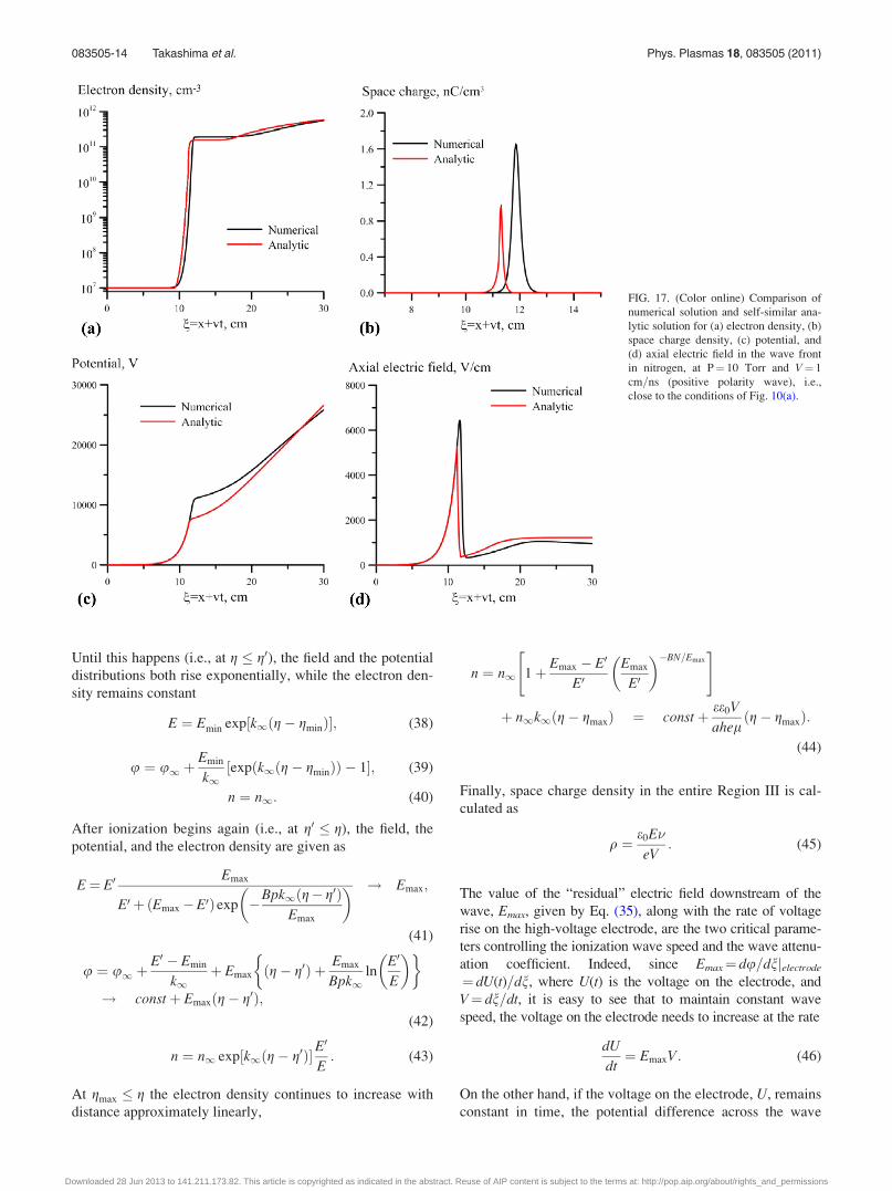
FIG. 17. (Color online) Comparison of

numerical solution and self-similar ana-

lytic solution for (a) electron density, (b)

space charge density, (c) potential, and

(d) axial electric field in the wave front

in nitrogen, at P¼ 10 Torr and V¼ 1

cm=ns (positive polarity wave), i.e.,

close to the conditions of Fig. 10(a).

083505-14 Takashima et al. Phys. Plasmas 18, 083505 (2011)

Downloaded 28 Jun 2013 to 141.211.173.82. This article is copyrighted as indicated in the abstract. Reuse of AIP content is subject to the terms at: http://pop.aip.org/about/rights_and_permissions

will decrease with distance, with the relative attenuation

coefficient of

d ¼ 1

ududn¼ Emax

U: (47)

4. Breakdown field near electrode and initialwave speed

For a Gaussian high-voltage pulse, given by Eq. (1),

breakdown field near the high-voltage electrode and the ini-

tial wave speed are given as follows:

�i;br

Ebr

Bp¼ 2f ln

2f e0

eln0

1

1þ Ebr

Bp

!;Ubr ¼

Ebr

k0

(48)

Vbr ¼2f

k0

1

1þ Ebr

Bp

; (49)

where Ubr is breakdown voltage

Ubr ¼ Upeak exp � t0 � tbr

s

� �2� �

;

f ¼ 1

Ubr

dUbr

dt¼ 2ðt0 � tbrÞ

s2;

(50)

and tbr is breakdown time. Note, however, that Eqs. (48),

(49) can be used only as estimates since in reality breakdown

near the electrode may strongly depend on the electrode ge-

ometry and surface material.

Summarizing, key results characterizing fast ionization

wave propagation include

(a) peak electric field in the primary ionization wave front,

E*, and potential difference across the primary wave, u*

(“breakdown potential” of the primary wave), Eq. (17)

(b) electron density after the primary ionization wave, n1,

Eq. (30)

(c) quasi-steady-state “residual” electric field achieved in

the secondary ionization wave, Emax, Eq. (35)

(d) electron density rise rate in the secondary ionization

wave, dn=dg, Eq. (44)

(e) voltage rise rate on the high-voltage electrode to main-

tain constant wave speed, dU=dt, Eq. (46)

(f) wave relative attenuation coefficient if the voltage on the

electrode remains constant, d, Eq. (47)

To illustrate the accuracy of the present self-similar ana-

lytic solution, Fig. 17 compares a numerical solution of Eqs.

(20)–(40) and an analytic solution for the electron density,

space charge density, potential, and axial electric field in the

positive polarity ionization wave in nitrogen at P¼ 10 Torr

and V¼ 1 cm=ns. This corresponds to the experimental con-

ditions of Fig. 10(a), i.e., positive polarity wave in nitrogen,

P¼ 10 Torr, �¼ 20 Hz, UDC¼ 760 V, and nearly constant

wave speed of V¼ 1.02 cm=ns at x¼ 11–25 cm. From

Fig. 17, it can be seen that the analytic solution is in good

agreement with the exact numerical solution. The model

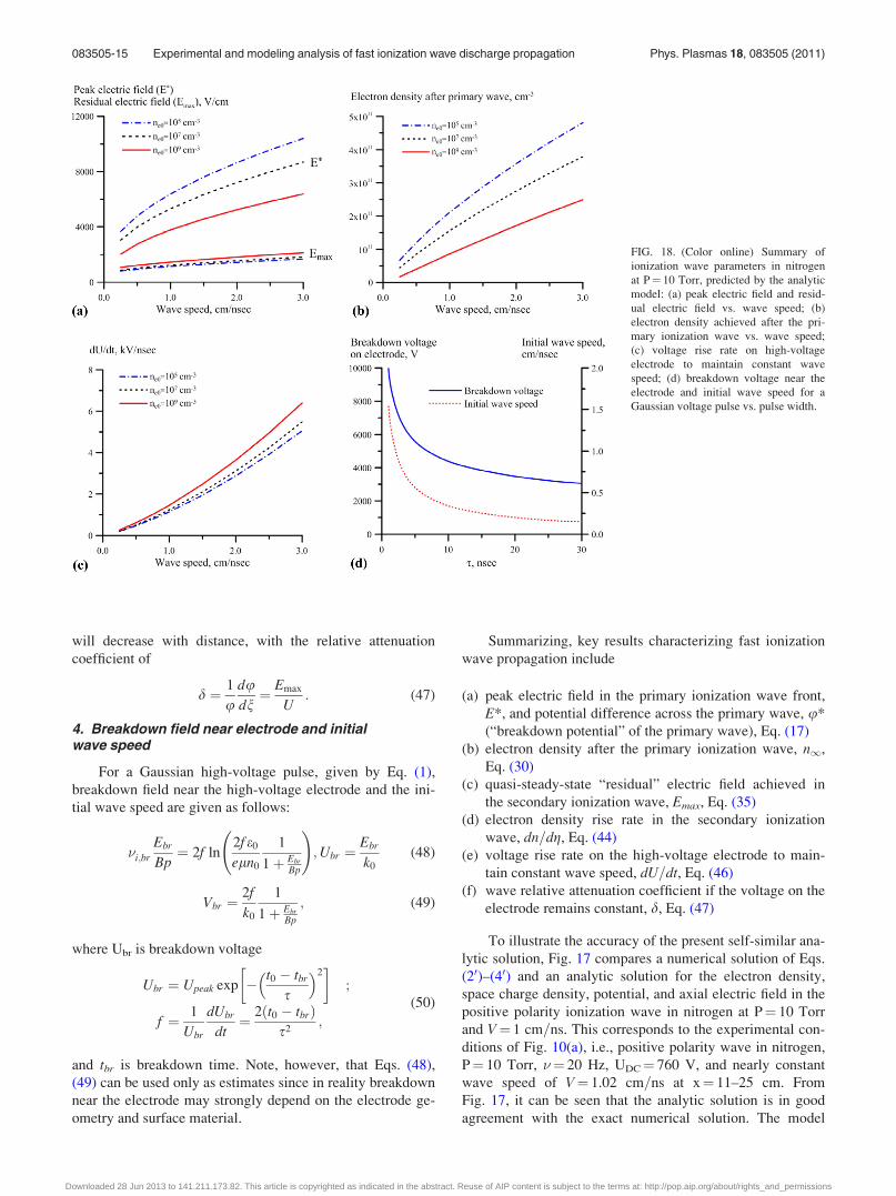
FIG. 18. (Color online) Summary of

ionization wave parameters in nitrogen

at P¼ 10 Torr, predicted by the analytic

model: (a) peak electric field and resid-

ual electric field vs. wave speed; (b)

electron density achieved after the pri-

mary ionization wave vs. wave speed;

(c) voltage rise rate on high-voltage

electrode to maintain constant wave

speed; (d) breakdown voltage near the

electrode and initial wave speed for a

Gaussian voltage pulse vs. pulse width.

083505-15 Experimental and modeling analysis of fast ionization wave discharge propagation Phys. Plasmas 18, 083505 (2011)

Downloaded 28 Jun 2013 to 141.211.173.82. This article is copyrighted as indicated in the abstract. Reuse of AIP content is subject to the terms at: http://pop.aip.org/about/rights_and_permissions

somewhat underestimates peak electric field, peak space

charge density, and the potential difference across the pri-

mary wave. However, the shape of the electron density, elec-

tric field, and potential distributions are reproduced fairly

well. In particular, the rate of electron density rise in the sec-

ondary ionization wave, as well as the residual electric field

and the wave attenuation coefficient given by the numerical

model and the analytic solution are close.

Figure 18(a) plots peak electric field in the wave front,

E*, and the residual electric field, Emax, vs. wave speed, V, for

different initial electron densities in the channel. As expected,

wave speed, which is controlled primarily by the rate of ioni-

zation in the wave front, �i (see Eq. (17)), has a strong (expo-

nential) dependence on E*. In other words, E* has logarithmic

dependence on wave speed. Although peak electric field also

has a relatively weak (double logarithmic) dependence on the

initial electron density, n0, it can be seen that increasing n0 by

several orders of magnitude reduces the peak field signifi-

cantly. Finally, Eq. (17) shows that peak electric field in the

wave front in fact depends on the product of the wave speed,

V, and the wavenumber, k0, which is controlled by the channel

geometry and by the dielectric constant (see Eq. (20)). There-

fore reducing the channel height, 2a, and the distance between

the waveguide plates, 2h, as well as increasing the dielectric

constant, e, may substantially increase peak electric field in the

wave. The residual electric field, Emax, given by Eq. (35) also

exhibits a weak logarithmic dependence on wave speed and is

nearly unaffected by the initial electron density.

Figure 18(b) shows that the electron density after the

primary ionization wave, n1, given by Eq. (30), increases

with the wave speed almost linearly. In fact, it is propor-

tional to the product Vk0, and therefore the electron density

can also be increased by reducing the waveguide transverse

dimensions and by using a dielectric with higher e. At higher

initial electron densities, n1 is reduced significantly because

charge separation in the wave front and self-shielding of the

plasma occur more rapidly, thereby terminating ionization

behind the wave front sooner.

Figure 18(c) demonstrates that maintaining higher wave

speeds requires higher rate of voltage rise on the high-voltage

electrode, dU=dt (see Eq. (45)). Since the residual electric

field, Emax, given by Eq. (35), exhibits relatively weak de-

pendence on wave speed and initial electron density (see Fig.

18(a)), dU=dt is the most critical parameter which controls

wave speed. The present results predict that maintaining ioni-

zation wave speeds of V¼ 1–3 cm=ns in nitrogen requires

rates of voltage increase of dU=dt� 1–5 kV=ns. Finally, Fig.

18(d) plots estimated initial breakdown field and initial wave

speed at its origin near the high-voltage electrode, predicted

by Eqs. (48) and (49), vs. voltage pulse width, s, for a Gaus-

sian shape voltage pulse given by Eq. (1). It can be seen that a

shorter voltage pulse (with a higher dU=dt) capable of main-

taining a high-speed ionization wave also needs to have higher

amplitude to generate breakdown near the electrode.

V. SUMMARY

In the present work, fast ionization wave discharges

propagating along a rectangular geometry channel=plasma

waveguide in nitrogen and helium are studied experimentally

and using kinetic modeling. The repetitive nanosecond pulse

discharge in the rectangular cross section channel was gener-

ated using a custom built pulsed plasma generator (peak volt-

age 10–40 kV, pulse duration 30–100 ns, voltage rise time

�1 kV=ns), generating a sequence of alternating polarity

high-voltage pulses at a pulse repetition rate of 20 Hz. Using

this plasma generator, both negative polarity and positive po-

larity ionization waves can be studied at the same experi-

mental conditions, using a low-jitter output trigger produced

by the generator on either positive or negative polarity

pulses. The ionization wave speed, as well as time-resolved

potential distributions and axial electric field distributions in

the propagating FIW discharge have been inferred from the

capacitive probe data. The probe is calibrated using voltage

pulses of known pulse shape and amplitude.

The experiments have been conducted in helium and

nitrogen, at pressures of 10–20 Torr, at pulse peak voltages

of 10–30 kV. As expected, wave speed increases with pulse

peak voltage, as voltage rise time on the high-voltage elec-

trode is reduced. Both the wave speed and the wave ampli-

tude (peak axial electric field in the wave front) for the

positive polarity wave exceed those for the negative polarity

wave. ICCD camera images demonstrate that the ionization

wave discharges in helium appear diffuse and volume-filling,

although emission intensity in the negative polarity wave is

higher near the top and bottom walls of the channel. On the

other hand, ionization wave discharges in nitrogen propagate

essentially along the walls of the discharge channel.

FIW discharge propagation has been analyzed numeri-

cally, using quasi-one-dimensional and two-dimensional ki-

netic models in a hydrodynamic (drift-diffusion), local

ionization approximation. The wave speed and the electric

field distribution in the wave front predicted by the model

are in good agreement with the experimental results in nitro-

gen. A self-similar analytic solution of the fast ionization

wave propagation equations has also been obtained. The ana-

lytic model of the FIW discharge predicts key ionization

wave parameters, such as wave speed, peak electric field in

the front, potential difference across the wave, and electron

density as functions of the waveform on the high voltage

electrode, in good agreement with the numerical calculations

and the experimental results.

ACKNOWLEDGMENTS

This work has been supported by the U.S. Department

of Energy Plasma Science Center, by the Department of

Physics and Astronomy of the Ruhr-University Bochum, and

by the Research Department “Plasmas with Complex Inter-

actions” of the Ruhr-University Bochum. We are grateful to

Dr. Mikhail Shneider from Princeton University for helpful

technical discussions. We would also like to thank Bernd

Becker, Frank Kremer, Stefan Wietholt, and Thomas Zierow

for their help with the experimental apparatus.

1L. M. Vasilyak, S. V. Kostyuchenko, N. N. Kudryavtsev, and I. V. Filyu-

gin, Phys.–Uspekhi 37, 247 (1994).2N. B. Anikin, S. V. Pancheshnyi, S. M. Starikovskaia, and A. Yu. Stari-

kovskii, J. Phys. D: Appl. Phys. 31, 826 (1998).

083505-16 Takashima et al. Phys. Plasmas 18, 083505 (2011)

Downloaded 28 Jun 2013 to 141.211.173.82. This article is copyrighted as indicated in the abstract. Reuse of AIP content is subject to the terms at: http://pop.aip.org/about/rights_and_permissions

3N. B. Anikin, S. M. Starikovskaia, and A. Yu. Starikovskii, J. Phys. D:

Appl. Phys. 34, 177 (2001).4N. B. Anikin, S. M. Starikovskaia, and A. Yu. Starikovskii, J. Phys. D:

Appl. Phys. 35, 2785 (2002).5N. B. Anikin, N. A. Zavialova, S. M. Starikovskaia, and A. Yu. Starikov-

skii, IEEE Trans. Plasma Sci. 36, 902 (2008).6S. V. Pancheshnyi, S. M. Starikovskaia, and A. Yu. Starikovskii, J. Phys.

D: Appl. Phys. 32, 2219 (1999).7S. V. Pancheshnyi, S. M. Starikovskaya, and A. Yu. Starikovskii, Plasma

Phys. Rep. 25, 393 (1999).8S. M. Starikovskaia, N. B. Anikin, S. V. Pancheshnyi, D. V. Zatsepin, and

A. Yu. Starikovskii, Plasma Sources Sci. Technol. 10, 344 (2001).9I. Gallimberti, J. Phys. D: Appl. Phys. 5, 2179 (1972).

10N. Yu. Babaeva and G. V. Naidis, Phys. Lett. A 215, 187 (1996).11E. M. van Veldhuizen and W. R. Rutgers, J. Phys. D: Appl. Phys. 35, 2169

(2002).12S. Pancheshnyi, M. Nudnova, and A. Starikovskii, Phys. Rev. E 71,

016407 (2005).13S. V. Pancheshnyi, S. M. Starikovskaia, and A. Yu. Starikovskii, J. Phys.

D: Appl. Phys. 32, 2219 (1999).

14L. D. Tsendin, “Principles of the electron kinetics in glow discharges,” in

Electron Kinetics and Applications of Glow Discharges, NATO ASI Se-

ries, Series B: Physics, edited by U. Kortshagen and L. D. Tsendin

(Kluwer, New York, 1998), Vol. 367, pp. 1–18.15E. Dewald, M. Gansiu, N. B. Mandache, G. Musa, M. Nistor, A. M.

Pointu, I.-I. Popescu, K. Frank, D. H. H. Hoffmann, and R. Stark, IEEE

Trans. Plasma Sci. 25, 279 (1997).16S. M. Starikovskaia, A. Yu. Starikovskii, and D. V. Zatsepin, J. Phys. D:

Appl. Phys. 31, 1118 (1998).17E. I. Asinovsky, A. N. Lagarkov, V. V. Markovets, and I. M. Rutkevich,

Plasma Sources Sci. Technol. 3, 556 (1994).18M. Nishihara, K. Udagawa Takashima, J. R. Bruzzese, I. V. Adamovich,

and D. Gaitonde, J. Propul. Power 27, 467 (2011).19A. N. Lagarkov and I. M. Rutkevich, Ionization Waves in Electric Break-

down of Gases (Springer, New York, 1994), Chap. 4.20Yu. P. Raizer, Gas Discharge Physics (Springer, Berlin, 1991), Chap.

2,4.21M. J. Kushner, J. Appl. Phys. 95, 846 (2004).22Z. Xiong and M. J. Kushner, J. Phys. D: Appl. Phys. 43, 505204

(2010).

083505-17 Experimental and modeling analysis of fast ionization wave discharge propagation Phys. Plasmas 18, 083505 (2011)

Downloaded 28 Jun 2013 to 141.211.173.82. This article is copyrighted as indicated in the abstract. Reuse of AIP content is subject to the terms at: http://pop.aip.org/about/rights_and_permissions