Embed Size (px)
Citation preview

International Journal of Oceanography & Aquaculture
Experimental Verification of Wave Breaking Formulae for Obliquely Incident Waves on Mixed and Gravel Beaches Int J Oceanogr Aquac
Experimental Verification of Wave Breaking Formulae for
Obliquely Incident Waves on Mixed and Gravel Beaches
Antoniadis C*
Coastal and Port Engineer/Rogan & Associates S.A., Athens, Greece
*Corresponding author: Christos Antoniadis, Coastal and Port Engineer/Rogan &
Associates S.A., Athens, Greece, Tel: 00306945042257; E-mail: [email protected]
Abstract
Wave breaking is the dominant process in the dynamics of near shore water movements resulting in sediment transport.
The transformation of the subsequent particle motion from irrotational to rotational motion generates vorticity and
turbulence and this affects the sediment transport. An improved understanding of the location of the breaker point and
characteristics of the wave under these changing parameters is essential to our understanding of short and long-term
morphological beach development.
This paper reports a series of 3-dimensional physical model tests to measure cross-shore and longshore current data,
generated by oblique wave attack, along gravel and mixed beaches with a uniform slope and a trench. The studies
described in this paper aim to improve the formulae derived by Longuet-Higgins and modified by Komar to predict the
longshore current velocity at the breaking point [1,2]. New formulae for predicting the wave breaking indices under these
conditions are proposed.
Keywords: Obliquely Incident Waves; Gravel Beaches; Wave Breaking
Introduction
Wave breaking at the shoreline is one of the least well understood of the coastal processes. There have been many stages and advances in our understanding of wave breaking, and these come predominantly from 2-dimensional physical model studies. To extend our understanding within the coastal environment a 3-dimensional physical model (Figure 1 & 2, Tables 1 & 2) was used to examine wave breaking formulae for obliquely incident waves on mixed and gravel beaches [3].
Figure 1: Position of the beach model.
Research Article
Volume 2 Issue 1
Received Date: December 20, 2017
Published Date: January 22, 2018

International Journal of Oceanography & Aquaculture
Antoniadis C. Experimental Verification of Wave Breaking Formulae for Obliquely Incident Waves on Mixed and Gravel Beaches. Int J Oceanogr Aquac 2018, 2(1): 000127.
Copyright© Antoniadis C.
2
Figure 2: Model bathymetry (trench, uniform slope) and location of measurements.
Type of Beach
D5 (mm)
D15
(mm) D16
(mm) D50
(mm) D84
(mm) D85
(mm) D90
(mm) D94
(mm)
Gravel Beach (G)
15.35 16.66 16.83 22.76 28.38 28.86 29.59 30.50
Mixed Beach (M)
0.21 0.32 0.33 12 25.20 25.9 27.31 29.19
Table 1: The different particle sizes of the sediments.
TESTS (Regular Waves)
Wave Height
(H)
Wave Period
(T)
TESTS (Random Waves)
Significant Wave
Height (Hm0)
Spectral Peak
Period (Tp)
Test 1-G 25.3 cm 2 sec Test 5-G 10.8 cm 2.3 sec Test 2-G 21.8 cm 3 sec Test 6-G 11 cm 3.2 sec Test 3-G 8.6 cm 2 sec Test 9-M 11 cm 2.3 sec Test 4-G 9.2 cm 3 sec Test 10-M 11.7 cm 3.1 sec
Test 7-M 8.6 cm 2 sec
Test 8-M 7.7 cm 3 sec
Table 2: Test programme of the experiments. Wave breaking depends on the nature of the bottom slope and the characteristics of the wave. Waves break as they reach a limiting steepness which is a function of the relative depth (d/L) and the beach slope (tanβ). Wave breaking may be classified in four types [4]: as spilling, plunging, collapsing, and surging. Breaker type may be identified according to the surf similarity parameter (Iribarren number) ξ0, defined as:
ξ0 =tanβ
HoLo
(1)
Where the subscript 0 denotes the deepwater condition [4,5]. On a uniformly sloping beach, breaker type is estimated by: Surging/collapsing ξ0>3.3 Plunging 0.5<ξ0<3.3 and,
Spilling ξ0<0.5 Furthermore, the depth (dB) and the height (HB) of breaking waves are important factors. The term “breaker index” is used to describe non-dimensional breaker height. The four common indices are in the form of Hb/db, Hb/H0, Hb/Lb and Hb/L0 (where the subscript b denotes the breaking condition). The first two indices are the breaker depth index (γ) and the breaker height index (Ωb), respectively. Rattanapitikon and Shibayama [6] examined the applicability of 24 existing formulas, for computing breaking wave height of regular wave, by wide range and large amount of published laboratory data (574 cases collected from 24 sources). They found that the formula of Komar and Gaughan [7] gives the best prediction, among 24 existing formulas, over a wide range of experiments. Komar and Gaughan [7] used linear wave theory to derive the breaker height formula from energy flux conservation and assumed a constant Hb/db. After calibrating the formula to the laboratory data of Iversen [8], Galvin [9], unpublished data of Komar and Simons and the field data of Munk [10], the formula proposed was:
𝐇𝐛 = 𝟎.𝟓𝟔𝐇𝐨 𝐇𝟎′
𝐋𝐨 −
𝟏
𝟓 𝐨𝐫 𝛀𝐛 = 𝟎.𝟓𝟔 𝐇𝟎′
𝐋𝐨 −
𝟏
𝟓 (2)
Where Ho
/ is the equivalent unrefracted deepwater wave height. Rattanapitikon and Shibayama [6] showed that the ER (root mean square relative error) of most formulae varies with the bottom slope, and it was expected that incorporating the new form of bottom slope effect into the formulas could improve the accuracy of the formulae. They therefore modified the three most accurate prediction formulae, concluding that the modified formula of Goda [11] gives the best prediction for the general case (ER=10.7%). The formula of Goda (1970) was modified to be:
𝐇𝐛 = 𝟎.𝟏𝟕𝐋𝟎 𝟏 − 𝐞𝐱𝐩 𝛑𝐝𝐛
𝐋𝐨 𝟏𝟔.𝟐𝟏 𝐭𝐚𝐧𝛃 𝟐 − 𝟕.𝟎𝟕𝐭𝐚𝐧𝛃 −
𝟏.𝟓𝟓 (3) The breaking depth, and consequently the breaking point, is also determined by using the Eq. (3) together with the linear wave theory. It is necessary that the breaking point is predicted accurately, in order for an accurate computation of the wave field or other wave-induced phenomena (e.g., undertow, sediment transport and beach deformation) to be concluded.
International Journal of Oceanography & Aquaculture
Antoniadis C. Experimental Verification of Wave Breaking Formulae for Obliquely Incident Waves on Mixed and Gravel Beaches. Int J Oceanogr Aquac 2018, 2(1): 000127.
Copyright© Antoniadis C.
3
It is well known that the wave height, just before the breaking point, is underestimated by linear wave theory. Consequently, the predicted breaking point will shift on shoreward of the real one when the breaker height formula is used together with the linear wave shoaling [12]. As a result, the computation of wave height transformation will not be predicted accurately. Two methods are known for dealing with the problem of underestimating the linear wave theory. The first method computes wave shoaling by using nonlinear wave theories [13-16] and the second method by using linear wave theory. The second method also uses other variables, rather than breaker height, to compute the breaking point [12,17-19]. Rattanapitikon and Shibayama [19], by following the second method, undertook a study to find out the suitable breaking wave formulas for computing breaker depth, and corresponding assumed orbital to phase velocity ratio and breaker height converted with linear wave theory. A total of 695 cases collected from 26 sources of published laboratory data were used. All data referred to experiments that were performed on regular waves. The formulae of Rattanapitikon and Shibayama gave satisfactory predictions over a wide range of experimental conditions. Their formulae for breaking depth and breaking wave height were:
hb = 3.86m2 − 1.98m + 0.88 H0 H0
L0 −0.16 for
H0
L0≤ 0.1
(4a)
hb = 3.86m2 − 1.98m + 0.88 H0 H0
L0 −0.34 for
H0
L0> 0.1
(4b) and
Hb = −0.57m2 + 0.31m + 0.58 L0 H0
L0 0.83 (5)
Where m is the bed slope. Random waves consist of incoming waves which have different wave height and they break in different water depths. Therefore, the wave breaking takes place in a relatively wide zone (surf zone) of variable water depth. Goda’s breaking method 20] is the most widely applied method for estimating significant wave heights (H1/3) within the surf zone. Goda [11] proposed a diagram, presenting criterion for predicting breaking wave height, based on the analysis of several sets of laboratory data of breaking waves on slopes obtained by several researchers [8,21,22]. Goda gave an approximate expression of the diagram as:
Hb = AL0 1 − exp −1.5πdb
Lo 1 + 15 tanβ
4
3 ] (6)
Where A= a coefficient (=0.12) The breaking point is defined as the maximum wave height admissible for a given water depth [23].
Calculation of the Long-Shore Velocity at the Breaking Point (vB)
The breaking of obliquely waves generates currents which usually dominate in and near the surf zone on open coasts. These wave driven currents have long-shore and cross-shore components. In this section, the long-shore velocity (vB) at the breaking point has been calculated in order to be compared with the results of the experimental tests for both gravel and mixed beaches. For the theoretical approximation of the vb the wave refraction and shoaling were included. Moreover, the seabed contours were assumed to be straight and parallel for both trench and beach with uniform slope. Despite the fact that trench usually does not have straight and parallel contour, this assumption was adopted. Moreover, approaches and equations that derived for planar beach, in their original form, were applied also at the trench. However, these approaches and equations, used for trench, were modified in order the effect of the complex sea bed contour to be reduced as more as possible.
Regular Waves
The following procedure relates to the estimation of breaking wave height and depth and is applied to regular waves. The deep water wavelength and celerity are calculated by:
L0 =C0
T (7)
C0 =gT
2π (8)
The water wavelength by,
L =gT2
2πtanh
2πd
L (9)
The shoaling coefficient KS and refraction coefficient KR can be estimated from,
KS = C0
C 2kd
sinh2kd]
1
2 (10)
and
KR = cosθ0
cosθ
1
2 (11)

International Journal of Oceanography & Aquaculture
Antoniadis C. Experimental Verification of Wave Breaking Formulae for Obliquely Incident Waves on Mixed and Gravel Beaches. Int J Oceanogr Aquac 2018, 2(1): 000127.
Copyright© Antoniadis C.
4
Where θ0 is the deepwater wave angle, where the wave number k is equal to 2π/L. Assuming that a refraction analysis gives a refraction coefficient KR at the point where breaking is expected to occur, and that the equivalent unrefracted deepwater wave height can be found from the refraction coefficient
𝐇𝐨′ = 𝐊𝐑𝐇𝟎, consequently 𝐇 = 𝐇𝐨′𝐊𝐒 (12)
Then by estimating the breaking wave height, the breaking depth can be calculated by corresponding equation. The initial value selected for the refraction coefficient would be checked to determine if it is correct for the actual breaker location. If necessary, a corrected refraction coefficient should be used to recompute the breaking wave height and depth. Longuet-Higgins [1] formed an expression for the mean longshore velocity (𝑣𝑙 ) at the breaker zone, of a planar beach, which was modified by Komar [2] and took the form of:
𝐯𝐥 = 𝟐.𝟕𝐮𝐛𝐬𝐢𝐧𝛉𝐛𝐜𝐨𝐬𝛉𝐛 (13)
Where θb= the wave angle at the breaking point ub= the wave orbital velocity under the wave breaking point, which is calculated by
𝐮𝐛 =𝛄
𝟐 𝐠𝐝𝐁 (14)
Where γ= breaking depth index (Hb/db) Longuet-Higgins [24] stated that the longshore velocity at the breaking point (vB) is usually about 0.2𝑣𝑙 . Therefore, knowing the breaking depth and height, the longshore velocity at the breaking point can be estimated by
𝐯𝐁 = 𝟎.𝟓𝟒𝛄
𝟐 𝐠𝐝𝐁𝐬𝐢𝐧𝛉𝐛𝐜𝐨𝐬𝛉𝐛 (15)
Moreover for a plane beach where d = xtanβ (tanβ is the beach slope), the distance to the breaker line from shore is
𝐱𝐁 =𝐝𝐁
𝐭𝐚𝐧𝛃 (16)
Using the above equations, vB was calculated for all the tests with regular waves. The slope between Lines 2 and 3 Figure 2 was approximately the same. Test 2 wasn’t taken into consideration for the calculations due to the fact that the slope changed significantly after Test 1. However, Eq. (14) was not based on a wave breaking equation that includes the influence of the slope.
Therefore, the three lines will be considered as one. The wave conditions for both gravel and mixed beaches were not exactly the same (except the Tests with wave height H=0.086m). Consequently, the longshore velocity at the breaking point would be similar for both types of beach, only in Tests 3 and 7. The results of the calculations are shown in Table 3.
Test (No.)
H
(m) T
(sec) Θ
(0) dB
(m) vB
(cm/s) 1 0.253 (G) 2 15 0.326 5.20 3 0.086 (G) 2 15 0.132 2.19 4 0.092 (G) 3 15 0.161 1.81 7 0.086 (M) 2 15 0.132 2.19 8 0.077 (M) 3 15 0.139 1.57
Table 3: The results of the calculations of vB for the tests with regular waves It has to be mentioned that the equation of Longuet-Higgins [24] did not take into consideration the spatial and temporal variability. The beach profile of each line has been changed through time due to the sediment transport. Therefore, the break point of each line changed and consequently vB changed. However, for the purpose of the comparison and the analysis of the equation of Longuet-Higgins [24], it was assumed that there were not any spatial and temporal variability. In order to compare the estimated values of vB with the measured vB from experimental results (for both types of beach), the data have been tabulated and presented in Table 4 and Table 5. It has to be mentioned that when the column of measured vB had negative values, it meant that the longshore current velocity was in opposite direction with the incoming wave direction and where the column has no number, it meant that there were no measurements (or measurements with less than 70% correlation) at that point.
Test (No.)
H
(m) T
(sec) dB
(m) vB (cm/s) estimated
vB (cm/s) measured
1 0.253 (L1) 2 0.326 5.20 2.36 1 0.253 (L2) 2 0.326 5.20 -4.85 1 0.253 (L3) 2 0.326 5.20 -6.52 3 0.086 (L1) 2 0.132 2.19 2.51 3 0.086 (L2) 2 0.132 2.19 7.45 3 0.086 (L3) 2 0.132 2.19 12.65 4 0.092 (L1) 3 0.161 1.81 -2.41 4 0.092 (L2) 3 0.161 1.81 0.26 4 0.092 (L3) 3 0.161 1.81 -
Table 4: The measured and estimated vB at the tests with gravel beach.

International Journal of Oceanography & Aquaculture
Antoniadis C. Experimental Verification of Wave Breaking Formulae for Obliquely Incident Waves on Mixed and Gravel Beaches. Int J Oceanogr Aquac 2018, 2(1): 000127.
Copyright© Antoniadis C.
5
Test (No.)
H
(m) T
(sec) dB
(m) vB (cm/s) estimated
vB (cm/s) measured
7 0.086 (L1) 2 0.131 2.18 - 7 0.086 (L2) 2 0.131 2.18 9.19 7 0.086 (L3) 2 0.131 2.18 - 8 0.077 (L1) 3 0.139 1.57 - 8 0.077 (L2) 3 0.139 1.57 - 8 0.077 (L3) 3 0.139 1.57 10.13
Table 5: The measured and estimated vB at the tests for the mixed beach The breaking longshore velocity has been chosen based on the value of the estimated breaking depth. It must be mentioned that the accuracy of the measurements of the ADV was ±0.5%. Looking at Table 4 and Table 5, the estimated vB from Longuet-Higgins [24] equation did not predict accurate results. Generally, it underestimated the measured vB. At some tests/lines the estimated vB was 9 times greater than the measured vB and at some other it was 7 times smaller. The estimated vB was similar to the measured vB,
only in Tests 1, 3 and 4 (especially for Line 1). At these tests, the magnitude of the vB was similar but not its direction. At the tests related to the mixed beach, there were only few available locations to compare with. Based on the theory that the longshore velocity at the breaking point would be the same for both types of beach, if both types of beach have the same wave conditions, the measured longshore velocity at the breaking point for Line 3 gave similar values for both types of beach for Tests 3 and 7. However, based on the assumption that the estimated breaking depth was accurate, it can be seen that the measured longshore “breaking” velocity had different values for all three lines. This happened due to the fact that the estimated vB of Longuet-Higgins [24] was based on a wave breaking equation that did not take into consideration the influence of the bottom slope (Hd=0.78db). Therefore, in order to include the influence of the bottom slope, the estimated breaking depth of Eq. (3) were used into Eq. (14). The longshore “breaking” velocities of Lines 2 and 3 were calculated as one due to the fact that the bottom slopes of both lines were approximately the same. At Line 1, where the trench was, the calculation of the breaking depth and consequently of vB based on different bottom slope from the other two Lines. The trench had two bottom slopes. The first slope was nearly horizontal. Based on the wave conditions in the tests, the first slope wouldn’t affect the breaking depth and breaking height. Therefore, the second bottom slope has been used for the
calculation of dB. As previously, Test 2 wasn’t considered in the calculations due to the fact that the bottom slope changed significantly after Test 1. The results of the calculations for Lines 2 and 3 are shown in Table 6.
Test (No.)
H
(m) T
(sec) θ
(0) ξ
dB (m)
vB (cm/s)
1 0.253 (G) 2 15 0.55 0.266 5.45 3 0.086 (G) 2 15 0.85 0.102 2.32 4 0.092 (G) 3 15 1.11 0.125 1.93 7 0.086 (M) 2 15 0.85 0.102 2.32 8 0.077 (M) 3 15 1.22 0.108 1.67
Table 6: The results of the calculations of vB for the tests with regular waves (Line 2 and Line 3) In order to compare the estimated values of vB with the measured vB from experimental results (for both types of beach), the data have been tabulated and presented in Table 7 and Table 8.
Test (No.)
H
(m) T
(sec) dB
(m) vB (cm/s) estimated
vB (cm/s) measured
1 0.253 (L2) 2 0.266 5.45 - 1 0.253 (L3) 2 0.266 5.45 -3.54 3 0.086 (L2) 2 0.104 2.31 - 3 0.086 (L3) 2 0.104 2.31 - 4 0.092 (L2) 3 0.125 1.93 6.31 4 0.092 (L3) 3 0.125 1.93 -
Table 7: The measured vB at the tests with gravel beach (Line 2 and Line 3)
Test (No.)
H
(m) T
(sec) dB
(m) vB (cm/s) estimated
vB (cm/s) measured
7 0.086 (L2) 2 0.102 2.32 - 7 0.086 (L3) 2 0.102 2.32 - 8 0.077 (L2) 3 0.108 1.67 - 8 0.077 (L3) 3 0.108 1.67 -
Table 8: The measured vB at the tests with mixed beach (Line 2 and Line 3) The results of the calculations for Line 1 are shown in Table 9.
Test (No.)
H
(m) T
(sec) θ
(0) ξ
dB (m)
vB (cm/s)
1 0.253 (G) 2 15 0.65 0.259 5.48 3 0.086 (G) 2 15 0.85 0.102 2.32 4 0.092 (G) 3 15 1.48 0.120 1.95 7 0.086 (M) 2 15 0.85 0.102 2.32 8 0.077 (M) 3 15 1.35 0.106 1.68
Table 9: The results for the calculations of vB for the tests with regular waves (Line 1)
International Journal of Oceanography & Aquaculture
Antoniadis C. Experimental Verification of Wave Breaking Formulae for Obliquely Incident Waves on Mixed and Gravel Beaches. Int J Oceanogr Aquac 2018, 2(1): 000127.
Copyright© Antoniadis C.
6
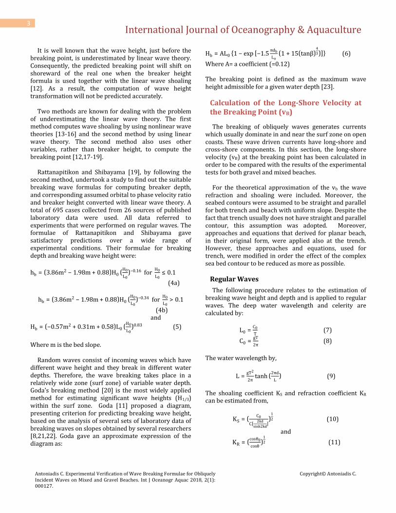
In order to compare the estimated values of vB with the measured vB from experimental results (for both types of beach), the data have been tabulated and presented in Table 10 and Table 11.
Test (No.)
H
(m) T
(sec) dB
(m) vB (cm/s) estimated
vB (cm/s) measured
1 0.253 2 0.259 5.48 - 3 0.086 2 0.102 2.32 - 4 0.092 3 0.120 1.95 -
Table 10: The measured vB at the tests with gravel beach (Line 1)
Test (No.)
H
(m) T
(sec) dB
(m) vB (cm/s) estimated
vB (cm/s) measured
7 0.086 2 0.102 2.32 - 8 0.077 3 0.106 1.68 -
Table 11: The measured vB at the tests with mixed beach (Line 1) Despite the fact that the new estimated vB had few available locations to compare with, especially for tests with mixed beach where there were not any measurements at these breaking depths for both trench and uniform slope, it gave slightly better results than the previous estimated vB of Longuet-Higgins equation. There were not any available measurements for trench for both types of beach. In general, the estimated value of vB was still not close enough to the measured vB. Rattanapitikon and Shibayama [19] undertook a study to find out the suitable breaking wave formulas for computing breaker depth, and corresponding orbital to phase velocity ratio and breaker height converted with linear wave theory. With regard to assumed orbital to phase velocity, only the formula of Isobe [12] was available. Rattanapitikon and Shibayama (2006) developed a new formula by reanalysis of the Isobe’s formula 12] . The new formula gave excellent predictions for all conditions (ERavg=3%). The assumed orbital velocity ( 𝑢𝑏 ) formula of Rattanapitikon and Shibayama [19] was written as:
𝐮𝐛 = −𝟎.𝟓𝟕𝐦𝟐+𝟎.𝟑𝟏𝐦+𝟎.𝟓𝟖 𝛑𝐜𝐛
𝐭𝐚𝐧𝐡𝟐 𝐤𝐛𝐡𝐛 𝐇𝟎
𝐋𝟎 𝟎.𝟖𝟑 (17)
Where, cb is the phase velocity at the breaking point, kb is the wave number at the breaking point, m is the bottom slope and hb is the breaker depth (Eq. 5). Eq. (14) was substituted by Eq.(17) in the Longuet-Higgins’s 24] equation. The new equation has the form of:
𝐯𝐥 = 𝟐.𝟕𝐮𝐛 𝐬𝐢𝐧𝛉𝐛𝐜𝐨𝐬𝛉𝐛 (18)
And consequently,
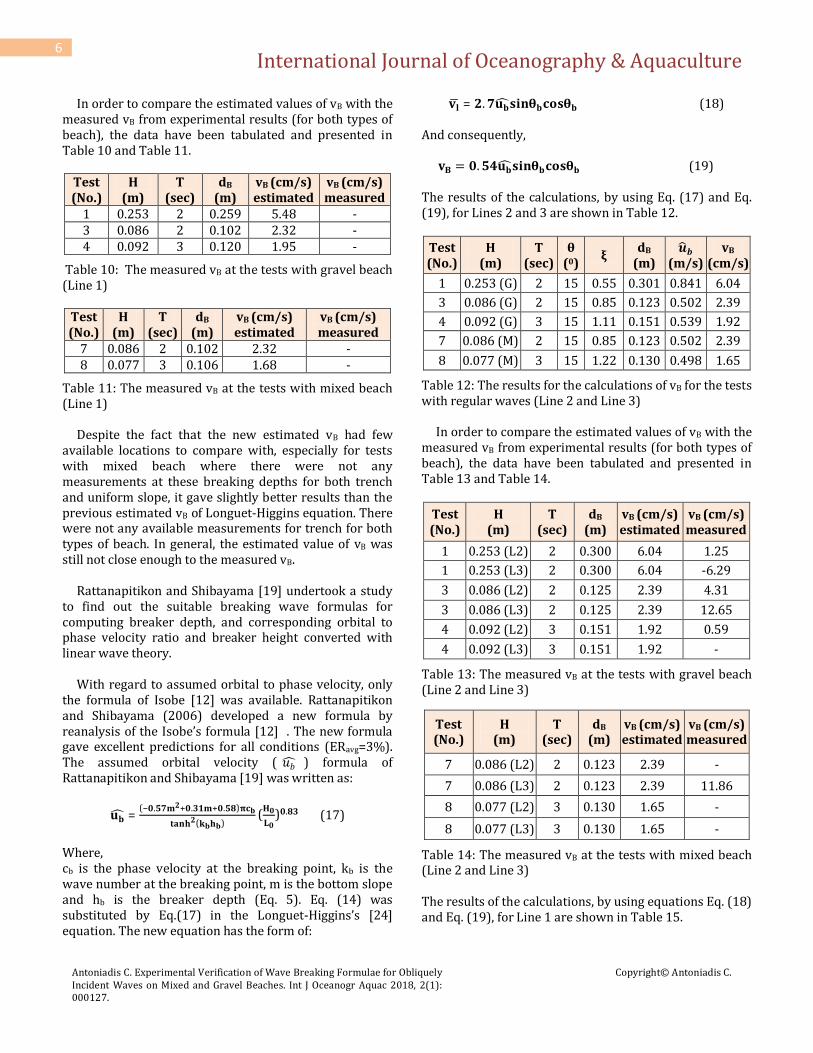
𝐯𝐁 = 𝟎.𝟓𝟒𝐮𝐛 𝐬𝐢𝐧𝛉𝐛𝐜𝐨𝐬𝛉𝐛 (19) The results of the calculations, by using Eq. (17) and Eq. (19), for Lines 2 and 3 are shown in Table 12.
Test (No.)
H
(m) T
(sec) θ
(0) ξ
dB (m)
𝒖 𝒃 (m/s)
vB (cm/s)
1 0.253 (G) 2 15 0.55 0.301 0.841 6.04
3 0.086 (G) 2 15 0.85 0.123 0.502 2.39
4 0.092 (G) 3 15 1.11 0.151 0.539 1.92
7 0.086 (M) 2 15 0.85 0.123 0.502 2.39
8 0.077 (M) 3 15 1.22 0.130 0.498 1.65
Table 12: The results for the calculations of vB for the tests with regular waves (Line 2 and Line 3) In order to compare the estimated values of vB with the measured vB from experimental results (for both types of beach), the data have been tabulated and presented in Table 13 and Table 14.
Test (No.)
H
(m) T
(sec) dB
(m) vB (cm/s) estimated
vB (cm/s) measured
1 0.253 (L2) 2 0.300 6.04 1.25
1 0.253 (L3) 2 0.300 6.04 -6.29
3 0.086 (L2) 2 0.125 2.39 4.31
3 0.086 (L3) 2 0.125 2.39 12.65
4 0.092 (L2) 3 0.151 1.92 0.59
4 0.092 (L3) 3 0.151 1.92 -
Table 13: The measured vB at the tests with gravel beach (Line 2 and Line 3)
Test (No.)
H
(m) T
(sec) dB
(m) vB (cm/s) estimated
vB (cm/s) measured
7 0.086 (L2) 2 0.123 2.39 -
7 0.086 (L3) 2 0.123 2.39 11.86
8 0.077 (L2) 3 0.130 1.65 -
8 0.077 (L3) 3 0.130 1.65 -
Table 14: The measured vB at the tests with mixed beach (Line 2 and Line 3) The results of the calculations, by using equations Eq. (18) and Eq. (19), for Line 1 are shown in Table 15.
International Journal of Oceanography & Aquaculture
Antoniadis C. Experimental Verification of Wave Breaking Formulae for Obliquely Incident Waves on Mixed and Gravel Beaches. Int J Oceanogr Aquac 2018, 2(1): 000127.
Copyright© Antoniadis C.
7
Test (No.)
H
(m) T
(sec) θ
(0) ξ
dB (m)
𝒖 𝒃 (m/s)
vB (cm/s)
1 0.253 (G) 2 15 0.65 0.292 0.856 6.07 3 0.086 (G) 2 15 0.85 0.123 0.502 2.39 4 0.092 (G) 3 15 1.48 0.144 0.557 1.94 7 0.086 (M) 2 15 0.85 0.123 0.502 2.39 8 0.077 (M) 3 15 1.35 0.127 0.504 1.66
Table 15: The results for the calculations of vB for the tests with regular waves (Line 1) In order to compare the estimated values of vB with the measured vB from experimental results (for both types of beach), the data have been tabulated and presented in Table 16 and Table 17.
Test (No.)
H
(m) T
(sec) dB
(m) vB (cm/s) estimated
vB (cm/s) measured
1 0.253 (L1) 2 0.291 6.07 7.95 3 0.086 (L1) 2 0.119 2.41 -1.86 4 0.092 (L1) 3 0.144 1.94 -
Table 16: The measured vB at the tests with gravel beach (Line 1)
Test (No.)
H
(m) T
(sec) dB
(m) vB (cm/s) estimated
vB (cm/s) measured
7 0.086 (L1) 2 0.123 2.39 - 8 0.077 (L1) 3 0.128 1.66 -
Table 17: The measured vB at the tests with mixed beach (Line 1) The values of estimated vB were close to the values of measured vB for Line 1 (for both types of beach) and for Line 3 (for gravel beach). It estimated quite accurately the magnitude of the vB for few tests. However, it also underestimated, as in the previous approaches, the value of vB in some occasions. Overall, Eq. (19) gave much more accurate results than the previous equations. Based on the experimental results and results of Eq. (19), two equations are proposed for estimation of the mean longshore velocity at the breaking point. A linear regression has been fitted to the data and the proposed fits are given by the following equations: For gravel beach-trench, 𝐯𝐁 = 𝟎.𝟓𝟓𝟒𝐮𝐛 𝐬𝐢𝐧𝛉𝐛𝐜𝐨𝐬𝛉𝐛 (20a)
For mixed beach-uniform slope 𝐯𝐁 = 𝟐.𝟔𝟖𝐮𝐛 𝐬𝐢𝐧𝛉𝐛𝐜𝐨𝐬𝛉𝐛 (20b)
Random Waves
The procedure of estimating the breaking wave height and depth for random waves is described in Appendix A. In this section, Eq. (19) was used to estimate the mean long-shore current at the breaking point as it was the most accurate equation for regular waves. However, the breaking depth will not be calculated by Eq. (4) but with Eq. (6). The results of the calculations, by using Eq. (19) with Eq. (6), for Lines 2 and 3 are shown in Table .
Test (No.)
H
(m) Ts
(sec) θ
(0) ξ
dB (m)
𝒖 𝒃 (m/s)
vB (cm/s)
5 0.108 (G) 2.26 15 0.77 0.183 0.696 3.72
6 0.110 (G) 3.24 15 1.10 0.222 0.852 3.53
9 0.110 (M) 2.28 15 0.86 0.179 0.724 3.81
10 0.117 (M) 3.05 15 1.45 0.200 0.964 4.03
Table 18: The results for the calculations of vB for the tests with random waves (Line 2 and Line 3) In order to compare the estimated values of vB with the measured vB from experimental results (for both types of beach), the data have been tabulated and presented in Table 19 and Table 20.
Test (No.)
H
(m) Ts
(sec) dB
(m) vB (cm/s) estimated
vB (cm/s) measured
5 0.108 (L2) 2.264 0.183 3.72 3.63
5 0.108 (L3) 2.264 0.183 3.72 2.04
6 0.110 (L2) 3.244 0.222 3.53 3.03
6 0.110 (L3) 3.244 0.222 3.53 3.05
Table 19: The measured vB at the tests with gravel beach (Line 2 and Line 3)
Test (No.)
H
(m) Ts
(sec) dB
(m) vB (cm/s) estimated
vB (cm/s) measured
9 0.110 (L2) 2.278 0.179 3.81 -
9 0.110 (L3) 2.278 0.179 3.81 -
10 0.117 (L2) 3.053 0.200 4.03 1.21
10 0.117 (L3) 3.053 0.200 4.03 1.95
Table 20: The measured vB at the tests with mixed beach (Line 2 and Line 3) The results of the calculations, by using Eq. (19) with Eq. (6), for Line1 are shown in Table 21.
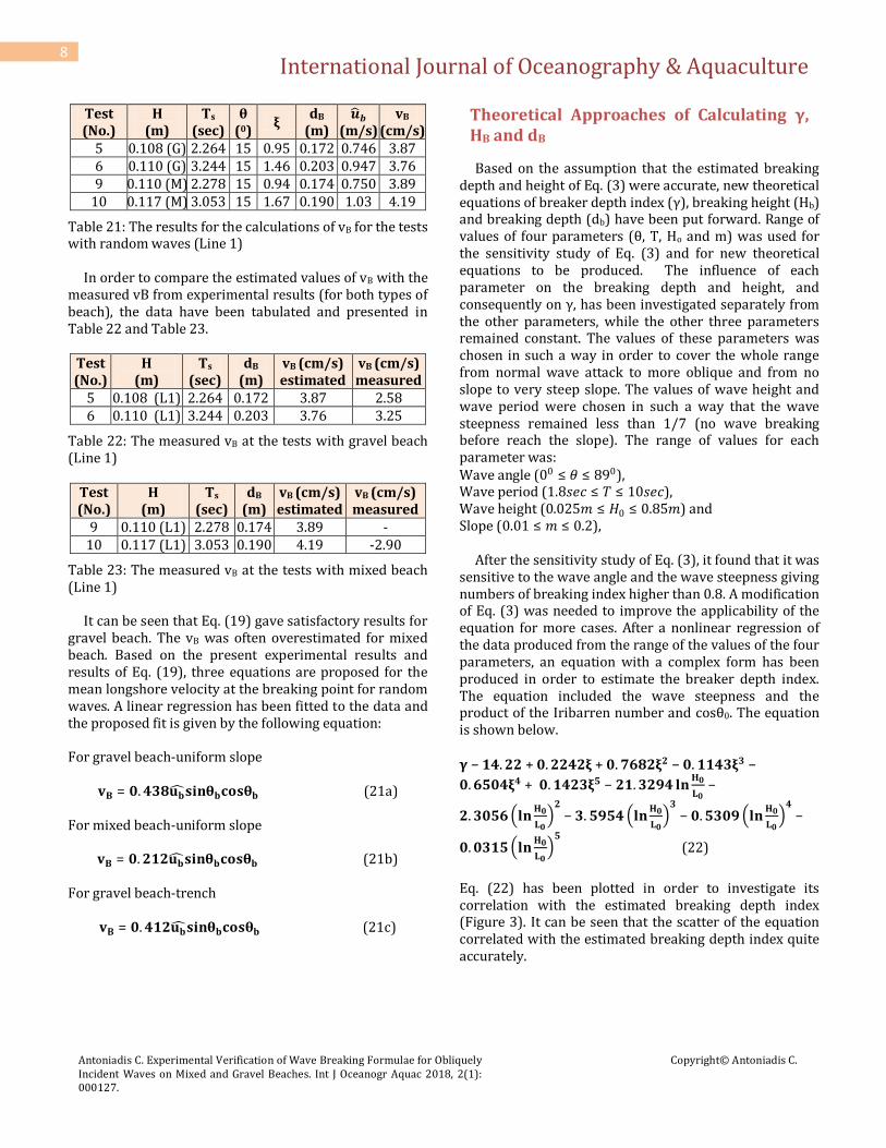
International Journal of Oceanography & Aquaculture
Antoniadis C. Experimental Verification of Wave Breaking Formulae for Obliquely Incident Waves on Mixed and Gravel Beaches. Int J Oceanogr Aquac 2018, 2(1): 000127.
Copyright© Antoniadis C.
8
Test (No.)
H
(m) Ts
(sec) θ
(0) ξ
dB (m)
𝒖 𝒃 (m/s)
vB (cm/s)
5 0.108 (G) 2.264 15 0.95 0.172 0.746 3.87 6 0.110 (G) 3.244 15 1.46 0.203 0.947 3.76 9 0.110 (M) 2.278 15 0.94 0.174 0.750 3.89
10 0.117 (M) 3.053 15 1.67 0.190 1.03 4.19
Table 21: The results for the calculations of vB for the tests with random waves (Line 1) In order to compare the estimated values of vB with the measured vB from experimental results (for both types of beach), the data have been tabulated and presented in Table 22 and Table 23.
Test (No.)
H
(m) Ts
(sec) dB
(m) vB (cm/s) estimated
vB (cm/s) measured
5 0.108 (L1) 2.264 0.172 3.87 2.58 6 0.110 (L1) 3.244 0.203 3.76 3.25
Table 22: The measured vB at the tests with gravel beach (Line 1)
Test (No.)
H
(m) Ts
(sec) dB
(m) vB (cm/s) estimated
vB (cm/s) measured
9 0.110 (L1) 2.278 0.174 3.89 - 10 0.117 (L1) 3.053 0.190 4.19 -2.90
Table 23: The measured vB at the tests with mixed beach (Line 1) It can be seen that Eq. (19) gave satisfactory results for gravel beach. The vB was often overestimated for mixed beach. Based on the present experimental results and results of Eq. (19), three equations are proposed for the mean longshore velocity at the breaking point for random waves. A linear regression has been fitted to the data and the proposed fit is given by the following equation: For gravel beach-uniform slope
𝐯𝐁 = 𝟎.𝟒𝟑𝟖𝐮𝐛 𝐬𝐢𝐧𝛉𝐛𝐜𝐨𝐬𝛉𝐛 (21a)
For mixed beach-uniform slope
𝐯𝐁 = 𝟎.𝟐𝟏𝟐𝐮𝐛 𝐬𝐢𝐧𝛉𝐛𝐜𝐨𝐬𝛉𝐛 (21b)
For gravel beach-trench
𝐯𝐁 = 𝟎.𝟒𝟏𝟐𝐮𝐛 𝐬𝐢𝐧𝛉𝐛𝐜𝐨𝐬𝛉𝐛 (21c)
Theoretical Approaches of Calculating γ, HB and dB
Based on the assumption that the estimated breaking depth and height of Eq. (3) were accurate, new theoretical equations of breaker depth index (γ), breaking height (Hb) and breaking depth (db) have been put forward. Range of values of four parameters (θ, T, Ho and m) was used for the sensitivity study of Eq. (3) and for new theoretical equations to be produced. The influence of each parameter on the breaking depth and height, and consequently on γ, has been investigated separately from the other parameters, while the other three parameters remained constant. The values of these parameters was chosen in such a way in order to cover the whole range from normal wave attack to more oblique and from no slope to very steep slope. The values of wave height and wave period were chosen in such a way that the wave steepness remained less than 1/7 (no wave breaking before reach the slope). The range of values for each parameter was: Wave angle (00 ≤ 𝜃 ≤ 890), Wave period (1.8𝑠𝑒𝑐 ≤ 𝑇 ≤ 10𝑠𝑒𝑐), Wave height (0.025𝑚 ≤ 𝐻0 ≤ 0.85𝑚) and Slope (0.01 ≤ 𝑚 ≤ 0.2), After the sensitivity study of Eq. (3), it found that it was sensitive to the wave angle and the wave steepness giving numbers of breaking index higher than 0.8. A modification of Eq. (3) was needed to improve the applicability of the equation for more cases. After a nonlinear regression of the data produced from the range of the values of the four parameters, an equation with a complex form has been produced in order to estimate the breaker depth index. The equation included the wave steepness and the product of the Iribarren number and cosθ0. The equation is shown below. 𝛄 − 𝟏𝟒.𝟐𝟐 + 𝟎.𝟐𝟐𝟒𝟐𝛏 + 𝟎.𝟕𝟔𝟖𝟐𝛏𝟐 − 𝟎.𝟏𝟏𝟒𝟑𝛏𝟑 −
𝟎.𝟔𝟓𝟎𝟒𝛏𝟒 + 𝟎.𝟏𝟒𝟐𝟑𝛏𝟓 − 𝟐𝟏.𝟑𝟐𝟗𝟒 𝐥𝐧𝐇𝟎
𝐋𝟎−
𝟐.𝟑𝟎𝟓𝟔 𝐥𝐧𝐇𝟎
𝐋𝟎 𝟐
− 𝟑.𝟓𝟗𝟓𝟒 𝐥𝐧𝐇𝟎
𝐋𝟎 𝟑
− 𝟎.𝟓𝟑𝟎𝟗 𝐥𝐧𝐇𝟎
𝐋𝟎 𝟒
−
𝟎.𝟎𝟑𝟏𝟓 𝐥𝐧𝐇𝟎
𝐋𝟎 𝟓
(22)
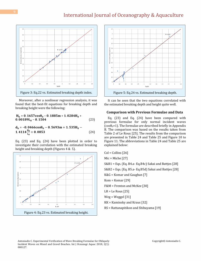
Eq. (22) has been plotted in order to investigate its correlation with the estimated breaking depth index (Figure 3). It can be seen that the scatter of the equation correlated with the estimated breaking depth index quite accurately.
International Journal of Oceanography & Aquaculture
Antoniadis C. Experimental Verification of Wave Breaking Formulae for Obliquely Incident Waves on Mixed and Gravel Beaches. Int J Oceanogr Aquac 2018, 2(1): 000127.
Copyright© Antoniadis C.
9
Figure 3: Eq.22 vs. Estimated breaking depth index. Moreover, after a nonlinear regression analysis, it was found that the best-fit equations for breaking depth and breaking height were the following: 𝐇𝐛 = 𝟎.𝟏𝟔𝟓𝟕𝐜𝐨𝐬𝛉𝟎 − 𝟎.𝟏𝟖𝟖𝟓𝐦 + 𝟏.𝟎𝟐𝟖𝟒𝐇𝟎 +𝟎.𝟎𝟎𝟏𝟖𝟗𝐋𝟎 − 𝟎.𝟏𝟓𝟎𝟒 (23) 𝐝𝐛 = −𝟎.𝟎𝟒𝟔𝟔𝐜𝐨𝐬𝛉𝟎 − 𝟎.𝟓𝟔𝟗𝟑𝐦+ 𝟏.𝟓𝟑𝟓𝐇𝟎 −
𝟏.𝟒𝟏𝟏𝟒𝐇𝟎
𝐋𝟎+ 𝟎.𝟎𝟖𝟓𝟑 (24)
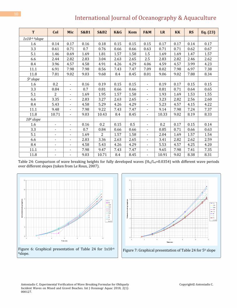
Eq. (23) and Eq. (24) have been plotted in order to investigate their correlation with the estimated breaking height and breaking depth (Figures 4 & 5).
Figure 4: Eq.23 vs. Estimated breaking height.
Figure 5: Eq.24 vs. Estimated breaking depth. It can be seen that the two equations correlated with the estimated breaking depth and height quite well.
Comparison with Previous Formulae and Data
Eq. (23) and Eq. (24) have been compared with previous formulae for only normal incident waves (cosθ0=1). The formulae are described briefly in Appendix B. The comparison was based on the results taken from Table 2 of Le Roux [25]. The results from the comparison are presented in Table 24 and Table 25 and Figure 10 to Figure 11. The abbreviations in Table 24 and Table 25 are explained below: Col = Collins [26]
Mic = Miche [27]
S&B1 = Eqs. (Eq. B4.a- Eq.B4c) Sakai and Battjes [28]
S&B2 = Eqs. (Eq. B5.a- Eq.B5d) Sakai and Battjes [28]
K&G = Komar and Gaughan [7]
Kom = Komar [29]
F&M = Frenton and McKee [30]
LR = Le Roux [25]
Weg = Weggel [31]
KK = Kaminsky and Kraus [32]
RS = Rattanapitikon and Shibayama [19]
International Journal of Oceanography & Aquaculture
Antoniadis C. Experimental Verification of Wave Breaking Formulae for Obliquely Incident Waves on Mixed and Gravel Beaches. Int J Oceanogr Aquac 2018, 2(1): 000127.
Copyright© Antoniadis C.
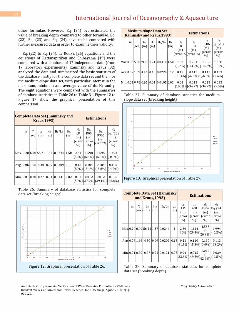
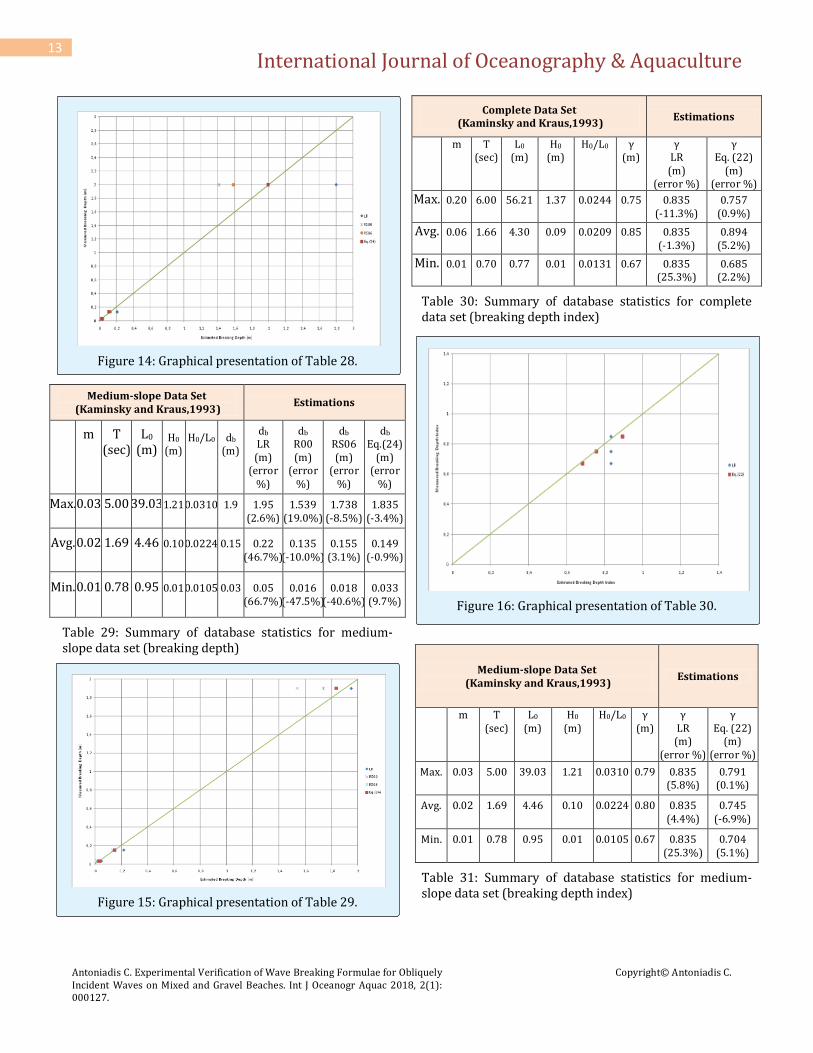
10
T Col Mic S&B1 S&B2 K&G Kom F&M LR KK RS Eq. (23)
1x10⁻⁶ 0slope
1.6 0.14 0.17 0.16 0.18 0.15 0.15 0.15 0.17 0.17 0.14 0.17
3.3 0.61 0.71 0.7 0.76 0.66 0.66 0.63 0.71 0.71 0.62 0.67
5.1 1.46 0.69 1.69 1.81 1.57 1.58 1.5 1.69 1.69 1.47 1.57
6.6 2.44 2.82 2.83 3.04 2.63 2.65 2.5 2.83 2.82 2.46 2.62
8.4 3.96 4.57 4.58 4.91 4.26 4.29 4.06 4.59 4.57 3.99 4.23
11.1 6.91 7.98 7.98 8.56 7.43 7.47 7.09 8.02 7.98 6.97 7.38
11.8 7.81 9.02 9.03 9.68 8.4 8.45 8.01 9.06 9.02 7.88 8.34
50 slope
1.6 0.2 - 0.16 0.19 0.15 0.15 - 0.19 0.17 0.15 0.15
3.3 0.84 - 0.7 0.81 0.66 0.66 - 0.81 0.71 0.64 0.65
5.1 2 - 1.69 1.95 1.57 1.58 - 1.93 1.69 1.53 1.55
6.6 3.35 - 2.83 3.27 2.63 2.65 - 3.23 2.82 2.56 2.60
8.4 5.43 - 4.58 5.29 4.26 4.29 - 5.23 4.57 4.15 4.22
11.1 9.48 - 7.98 9.22 7.43 7.47 - 9.14 7.98 7.24 7.37
11.8 10.71 - 9.03 10.43 8.4 8.45 - 10.33 9.02 8.19 8.33
100 slope
1.6 - - 0.16 0.2 0.15 0.5 - 0.2 0.17 0.15 0.14
3.3 - - 0.7 0.84 0.66 0.66 - 0.85 0.71 0.66 0.63
5.1 - - 1.69 2 1.57 1.58 - 2.04 1.69 1.57 1.54
6.6 - - 2.83 3.36 2.63 2.65 - 3.41 2.82 2.62 2.59
8.4 - - 4.58 5.43 4.26 4.29 - 5.53 4.57 4.25 4.20
11.1 - - 7.98 9.47 7.43 7.47 - 9.65 7.98 7.41 7.35
11.8 - - 9.03 10.71 8.4 8.45 - 10.91 9.02 8.38 8.31
Table 24: Comparison of wave breaking heights for fully developed waves (H0/L0=0.0354) with different wave periods over different slopes (taken from Le Roux, 2007).
Figure 6: Graphical presentation of Table 24 for 1x10⁻⁶ 0slope.
Figure 7: Graphical presentation of Table 24 for 50 slope

International Journal of Oceanography & Aquaculture
Antoniadis C. Experimental Verification of Wave Breaking Formulae for Obliquely Incident Waves on Mixed and Gravel Beaches. Int J Oceanogr Aquac 2018, 2(1): 000127.
Copyright© Antoniadis C.
11
Figure 8: Graphical presentation of Table 24 for 100 slope.
T Weg Kom LR KK RS Eq. (24)
1x10⁻⁶ 0slope
1.6 0.22 0 0.2 - 0.21 0.21
3.3 0.91 0.01 0.85 - 0.90 0.91
5.1 2.17 0.02 2.03 - 2.16 2.19
6.6 3.63 0.04 3.39 - 3.62 3.68
8.4 5.88 0.06 5.5 - 5.86 5.97
11.1 10.28 0.11 9.6 - 10.23 10.44
11.8 11.62 0.13 10.85 - 11.56 11.80
50 slope
1.6 0.18 0.15 0.16 0.17 0.18 0.16
3.3 0.77 0.64 0.69 0.72 0.76 0.86
5.1 1.83 1.52 1.65 1.71 1.81 2.15
6.6 3.07 2.55 2.77 2.86 3.03 3.63
8.4 4.97 4.13 4.49 4.64 4.90 5.93
11.1 8.69 7.2 7.83 8.10 8.56 10.39
11.8 9.82 8.14 8.85 9.15 9.67 11.75
100 slope
1.6 - 0.18 0.15 0.14 0.16 0.11
3.3 - 0.77 0.65 0.60 0.67 0.81
5.1 - 1.84 1.55 1.44 1.60 2.10
6.6 - 3.08 2.59 2.40 2.67 3.58
8.4 - 4.99 4.19 3.89 4.33 5.88
11.1 - 8.7 7.32 6.80 7.56 10.34
11.8 - 9.84 8.27 7.68 8.55 11.70
Table 25: Comparison of wave breaking depths for fully developed waves (H0/L0=0.0354) with different wave periods over different slopes [25].
Figure 9: Graphical presentation of Table 25 for 1x10⁻⁶ 0slope.
Figure 10: Graphical presentation of Table 25 for 50 slope.
Figure 11: Graphical presentation of Table 25 for 100 slope. As it can be seen, Eq. (23) slightly underestimated the value of breaking height compared to the values of the
International Journal of Oceanography & Aquaculture
Antoniadis C. Experimental Verification of Wave Breaking Formulae for Obliquely Incident Waves on Mixed and Gravel Beaches. Int J Oceanogr Aquac 2018, 2(1): 000127.
Copyright© Antoniadis C.
12
other formulae. However, Eq. (24) overestimated the value of breaking depth compared to other formulae. Eq. (22), Eq. (23) and Eq. (24) have to be compared with further measured data in order to examine their validity. Eq. 22 to Eq. 24 , Le Roux’s 25] equations and the equations of Rattanapitikon and Shibayama [19] were compared with a database of 17 independent data (from 17 laboratory experiments). Kaminsky and Kraus [32] analyzed the data and summarized the basic statistics of the database, firstly for the complete data set and then for the medium-slope data set, with particular interest in the maximum, minimum and average value of dB, HB and γ. The eight equations were compared with the summaries of database statistics in Table 26 to Table 31. Figure 12 to Figure 17 show the graphical presentation of this comparison.
Complete Data Set (Kaminsky and Kraus,1993)
Estimations
m
T (sec)
L0 (m)
H0 (m)
H0/L0
Hb (m)
Hb LR
(m) (error
%)
Hb R00 (m)
(error %)
Hb RS06 (m)
(error %)
Hb Eq. (23)
(m) (error
%)
Max.
0.20
6.00
56.21
1.37
0.0244
1.50
2.34 (56%)
1.598 (6.6%)
1.595 (6.3%)
1.493 (-0.5%)
Avg.
0.06
1.66
4.30
0.09
0.0209
0.11
0.18 (80%)
0.104 (-5.1%)
0.104 (-5.8%)
0.105 (-4.8%)
Min.
0.01
0.70
0.77
0.01
0.0131
0.02
0.03 (50%)
0.012 (37.7%)
0.012 (39.1%)
0.025 (25.8%)
Table 26: Summary of database statistics for complete data set (breaking height).
Figure 12: Graphical presentation of Table 26.
Medium-slope Data Set (Kaminsky and Kraus,1993)
Estimations
m
T (sec)
L0 (m)
H0 (m)
H0/L0
Hb (m)
Hb LR
(m) (error %)
Hb R00 (m)
(error %)
Hb RS06 (m)
(error %)
Hb Eq. (23)
(m) (error
%)
Max.
0.03
5.00
39.03
1.21
0.0310
1.50
1.63 (8.7%)
1.291 (-13.9%)
1.286 (-14.3%)
1.328 (-11.5%)
Avg.
0.02
1.69
4.46
0.10
0.0224
0.12
0.19 (58.3%)
0.112 (-6.5%)
0.112 (-6.5%)
0.123 (2.4%)
Min.
0.01
0.78
0.95
0.01
0.0105
0.02
0.04 (100%)
0.013 (-34.7%)
0.013 (-34.7%)
0.025 (27.5%)
Table 27: Summary of database statistics for medium-slope data set (breaking height)
Figure 13: Graphical presentation of Table 27.
Complete Data Set (Kaminsky and Kraus,1993)
Estimations
m
T (sec)
L0 (m)
H0 (m)
H0/L0
db (m)
db LR
(m) (error
%)
db R00 (m)
(error %)
db RS06 (m)
(error %)
db Eq. (24)
(m) (error
%)
Max.
0.20
6.00
56.21
1.37
0.0244
2
2.80 (40%)
1.414 (-29.3%)
1.585 (-
20.8%)
1.994 (-0.3%)
Avg.
0.06
1.66
4.30
0.09
0.0209
0.13
0.21 (61.5%)
0.110 (-15.3%)
0.130 (0.0%)
0.113 (-13.2%)
Min.
0.01
0.70
0.77
0.01
0.0131
0.03
0.04 (33.3%)
0.015 (-49.5%)
0.017 (-
42.6%)
0.029 (-2.5%)
Table 28: Summary of database statistics for complete data set (breaking depth)
International Journal of Oceanography & Aquaculture
Antoniadis C. Experimental Verification of Wave Breaking Formulae for Obliquely Incident Waves on Mixed and Gravel Beaches. Int J Oceanogr Aquac 2018, 2(1): 000127.
Copyright© Antoniadis C.
13
Figure 14: Graphical presentation of Table 28.
Medium-slope Data Set (Kaminsky and Kraus,1993)
Estimations
m
T (sec)
L0 (m)
H0 (m)
H0/L0
db (m)
db LR
(m) (error
%)
db R00 (m)
(error %)
db RS06 (m)
(error %)
db Eq.(24)
(m) (error
%)
Max.
0.03
5.00
39.03
1.21
0.0310
1.9
1.95 (2.6%)
1.539 (19.0%)
1.738 (-8.5%)
1.835 (-3.4%)
Avg.
0.02
1.69
4.46
0.10
0.0224
0.15
0.22 (46.7%)
0.135 (-10.0%)
0.155 (3.1%)
0.149 (-0.9%)
Min.
0.01
0.78
0.95
0.01
0.0105
0.03
0.05 (66.7%)
0.016 (-47.5%)
0.018 (-40.6%)
0.033 (9.7%)
Table 29: Summary of database statistics for medium-slope data set (breaking depth)
Figure 15: Graphical presentation of Table 29.
Complete Data Set (Kaminsky and Kraus,1993)
Estimations
m
T (sec)
L0 (m)
H0 (m)
H0/L0
γ (m)
γ LR
(m) (error %)
γ Eq. (22)
(m) (error %)
Max.
0.20
6.00
56.21
1.37
0.0244
0.75
0.835 (-11.3%)
0.757 (0.9%)
Avg.
0.06
1.66
4.30
0.09
0.0209
0.85
0.835 (-1.3%)
0.894 (5.2%)
Min.
0.01
0.70
0.77
0.01
0.0131
0.67
0.835 (25.3%)
0.685 (2.2%)
Table 30: Summary of database statistics for complete data set (breaking depth index)
Figure 16: Graphical presentation of Table 30.
Medium-slope Data Set (Kaminsky and Kraus,1993)
Estimations
m
T (sec)
L0 (m)
H0 (m)
H0/L0
γ (m)
γ LR
(m) (error %)
γ Eq. (22)
(m) (error %)
Max.
0.03
5.00
39.03
1.21
0.0310
0.79
0.835 (5.8%)
0.791 (0.1%)
Avg.
0.02
1.69
4.46
0.10
0.0224
0.80
0.835 (4.4%)
0.745 (-6.9%)
Min.
0.01
0.78
0.95
0.01
0.0105
0.67
0.835 (25.3%)
0.704 (5.1%)
Table 31: Summary of database statistics for medium-slope data set (breaking depth index)
International Journal of Oceanography & Aquaculture
Antoniadis C. Experimental Verification of Wave Breaking Formulae for Obliquely Incident Waves on Mixed and Gravel Beaches. Int J Oceanogr Aquac 2018, 2(1): 000127.
Copyright© Antoniadis C.
14
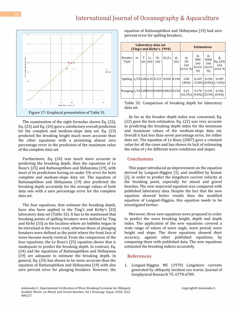
Figure 17: Graphical presentation of Table 31. The examination of the eight formulae shown Eq. (22), Eq. (23) and Eq. (24) gave a satisfactory overall prediction for the complete and medium-slope data set. Eq. (23) predicted the breaking height much more accurate than the other equations with a promising almost zero percentage error in the prediction of the maximum value of the complete data set. Furthermore, Eq. (24) was much more accurate in predicting the breaking depth, than the equations of Le Roux’s 25] and Rattanapitikon and Shibayama 19], with most of its predictions having an under 5% error for both complete and medium-slope data set. The equation of Rattanapitikon and Shibayama [19] also predicted the breaking depth accurately for the average values of both data sets with a zero percentage error for the complete data set. The four equations, that estimate the breaking depth, have also been applied to the Ting’s and Kirby’s 33] laboratory data set (Table 32). It has to be mentioned that breaking points of spilling breakers were defined by Ting and Kirby [33] as the location where air bubbles began to be entrained in the wave crest, whereas those of plunging breakers were defined as the point where the front face of wave became nearly vertical. From the comparison of the four equations, the Le Roux’s 25] equation shows that is inadequate to predict the breaking depth. In contrast, Eq. (24) and the equations of Rattanapitikon and Shibayama [19] are adequate to estimate the breaking depth. In general, Eq. (24) has shown to be more accurate than the equation of Rattanapitikon and Shibayama [19] with also zero percent error for plunging breakers. However, the
equation of Rattanapitikon and Shibayama [19] had zero percent error for spilling breakers.
Laboratory data set (Ting’s and Kirby’s, 1994)
Estimations
Breaker Type
m
T (sec)
L0 (m)
H0 (m)
H0/L0
db (m)
db LR (m)
(error %)
db R00 (m)
(error %)
db RS06 (m)
(error %)
db Eq. (24)
(m) (error %)
Spilling
1/35
2.00
6.25
0.127
0.020
0.196
2.80 (40%)
0.169 (-13.8%)
0.196 (0.0%)
0.189 (-3.6%)
Plunging
1/35
5.00
39.03
0.089
0.0023
0.156
0.21 (61.5%)
0.170 (9.0%)
0.195 (25.9%)
0.156 (0.0%)
Table 32: Comparison of breaking depth for laboratory data set. As far as the breaker depth index was concerned, Eq. (22) gave the best estimation. Eq. (22) was very accurate in predicting the breaking depth index for the minimum and maximum values of the medium-slope data set. Overall it had less than seven percentage error, for either data set. The equation of Le Roux (2007) gave a constant value for all the cases and has shown its lack of estimating the value of γ for different wave conditions and slopes.
Conclusions
This paper introduced an improvement on the equation derived by Longuet-Higgins [1], and modified by Komar [2], in order to predict the longshore current velocity at the breaking point, especially for mixed and gravel beaches. The new improved equation was compared with published laboratory data. Despite the fact that the new equation showed better results than the modified equation of Longuet-Higgins, this equation needs to be investigated further. Moreover, three new equations were proposed in order to predict the wave breaking height, depth and depth index. The application of the new equations covered a wide range of values of wave angle, wave period, wave height and slope. The three equations showed their accuracy, against other published equations, by comparing them with published data. The new equations estimated the breaking indices accurately.
References
1. Longuet-Higgins MS (1970) Longshore currents generated by obliquely incident sea waves. Journal of Geophysical Research 75: 6778-6789.
International Journal of Oceanography & Aquaculture
Antoniadis C. Experimental Verification of Wave Breaking Formulae for Obliquely Incident Waves on Mixed and Gravel Beaches. Int J Oceanogr Aquac 2018, 2(1): 000127.
Copyright© Antoniadis C.
15
2. Komar PD (1976) Beach Processes and Sedimentation. Prentice-Hall, Englewood Cliffs, NJ.
3. Antoniadis C (2009) Wave-induced currents and sediment transport on gravel and mixed beaches, PhD, Thesis, Cardiff University.
4. Galvin CJ (1968) Breaker Type Classification on Three Laboratory Beaches. Journal of Geophysical Research 73(12): 3651-3659.
5. Battjes JA (1974) Surf-Similarity. Proceedings of the 14th Coastal Engineering Conference, ASCE, pp: 466-480.
6. Rattanapitikon W, Shibayama T (2000) Verification and modification of breaker height formulas. Coastal Engineering Journal 42(4): 389-406.
7. Komar PD, Gaughan MK (1973) Airy wave theory and breaker height prediction. Proceedings of the 13th Coastal Engineering Conference, ASCE, pp: 405-418.
8. Iversen HW (1952) Laboratory study of breakers, Gravity Waves, Circular 52, US Bureau of Standards, pp: 9-32.
9. Galvin CJ (1969) Breaker travel and choice of design wave height. Journal of Waterway Harbors Div ASCE 95(2): 175-200.
10. Munk WH (1949) The solitary wave theory and its application to surf problems. Ann New York Acad Sci 51: 376-423.
11. Goda Y (1970) A synthesis of breaker indices. Trans JSCE 2: 227-230.
12. Isobe M (1987) A parabolic equation model for transformation of irregular waves due to refraction, diffraction and breaking. Coastal Engineering in Japan, JSCE 30(1): 33-47.
13. Stokes GG (1847) On the theory of oscillatory waves. Trans Camb Phil Soc 8: 411-455.
14. Dean RG (1965) Stream function representation of nonlinear ocean waves. Journal of Geophysical Research 70(18): 4561-4572.
15. Shuto N (1974) Non-linear long waves in channel of variable section. Coastal Engineering in Japan, JSCE 17: 1-12.
16. Isobe M (1985) Calculation and application of first-order cnodial wave theory. Coastal Engineering Journal 9(4): 309-325.
17. Watanabe A, Hara T, Horikawa K (1984) Study on breaking condition for compound wave trains. Coastal Engineering in Japan, JSCE 27: 71-82.
18. Rattanapitikon W (1995) Cross-Shore Sediment Transport and Beach Deformation Model. Dissertation, Dep Civil Engineering, Yokohama National University, Yokohama, Japan, pp: 90.
19. Rattanapitikon W, Shibayama T (2006) Breaking wave formulas for breaking depth and orbital to phase velocity ratio. Coastal Engineering Journal 48(4): 395-416.
20. Goda Y (1985) Random Seas and Design of Maritime Structures. University of Tokyo Press., Tokyo, pp: 464.
21. Mitsuyasu H (1962) Experimental study on wave force against a wall. Report of the Transportation Technical Research Institute 47: 39.
22. Goda Y (1964) Wave forces on a vertical circular cylinder: Experiments and a proposed method of wave force computation. Report of the Port and Harbor Research Institute, Ministry of Transportation 8: 74.
23. Torrini L, Allsop NWH (1999) Goda’s breaking prediction method- A discussion note on how this should be applied. HR Report, IT 473, Wallingford, U.K.
24. Longuet-Higgins MS (1972) Recent Progress in the Study of Longshore Currents. Waves on Beaches, Meyer RE (Ed.), New York: Academic Press, pp: 203-248.
25. Le Roux JP (2007) A simple method to determine breaker height and depth for different deepwater wave height/length ratios and sea floor slopes. Journal of Coastal Engineering 54: 271-277.
26. Collins IA (1970) Probability of breaking wave characteristics. In: Proc 12th Conf Coastal Engr, ASCE, pp: 199-414.
27. Miche R (1944) Mouvements ondulatoires des mers en profundeur constante on decroisante. Annales des Ponts et Chaussees, Chap114: 25-78, 131-164, 270-292,369-406.

International Journal of Oceanography & Aquaculture
Antoniadis C. Experimental Verification of Wave Breaking Formulae for Obliquely Incident Waves on Mixed and Gravel Beaches. Int J Oceanogr Aquac 2018, 2(1): 000127.
Copyright© Antoniadis C.
16
28. Sakai T, Battjes JA (1980) Wave theory calculated from Cokelet’s theory. Coastal Engineering 4: 65-84.
29. Komar PD (1998) Beach Processes and Sedimentation. Prentice Hall, Upper Saddle River, NJ 543.
30. Fenton JD, McKee WD (1990) On calculating the lengths of water waves. Coastal Engineering, 14(6): 499-513.
31. Weggel JR (1972) Maximum breaker height. J Waterw Harbors, Coastal Eng Div 529-548.
32. Kaminsky GM, Kraus CN (1993) Evaluation of depth-limited wave breaking criteria. Proc. of the 2nd International Symposium Ocean ’93 , WPCOD, ASCE, pp: 180-193.
33. Ting FCK, Kirby JT (1994) Observation of undertow and turbulence in a laboratory surf zone. Coastal Engineering 24: 51-80.
34. Cokelet ED (1977) Steep gravity waves in water of arbitrary uniform depth. Philos Trans R Soc Lond Ser A: Math Phys Sci, pp: 183-230.