Coastal Engineering 55 (2008) 741–752

Contents lists available at ScienceDirect

Coastal Engineering

j ourna l homepage: www.e lsev ie r.com/ locate /coasta leng

Experimental study of wave–wave nonlinear interactions using thewavelet-based bicoherence

Guohai Dong a,⁎, Yuxiang Ma a,⁎, Marc Perlin b, Xiaozhou Ma a, Bo Yu a, Jianwu Xu a

a State Key Laboratory of Coastal and Offshore Engineering, Dalian University of Technology, Dalian, 116023, PR Chinab Department of Naval Architecture and Marine Engineering, University of Michigan, Ann Arbor, Michigan, 48109 USA

a r t i c l e i n f o

⁎ Corresponding authors. Tel.: +86 411 84706213; faxE-mail addresses: ghdong@dlut.edu.cn (G. Dong), yu

0378-3839/$ – see front matter © 2008 Elsevier B.V. Aldoi:10.1016/j.coastaleng.2008.02.015

a b s t r a c t

Article history:Received 9 July 2007Received in revised form 17 December 2007Accepted 13 February 2008Available online 26 March 2008

The wavelet-based bicoherence, which is a new and powerful tool in the analysis of nonlinear phase coupling,is used to study the nonlinear wave–wave interactions of breaking and non-breaking gravity wavespropagating over a sill. Two cases of mechanically generated randomwaves based on JONSWAP spectra are usedfor this purpose. Values of relative depth, kph (kp is the wave number of the spectral peak and h is the waterdepth) for this study range between 0.38 and 1.22. The variations of wavelet-based total bicoherence for thetest cases indicate that the degree of quadratic phase coupling increases in the shoaling region consistent withawave profile that is pitched shoreward, relative to a vertical axis as seen in the experiments, but decreases inthe de-shoaling region. For the non-breaking case, the degree of quadratic phase coupling continues toincrease until waves reach the top of the sill. Breaking waves, however, achieve their highest level of quadraticphase coupling immediately before incipient breaking and the degree of phase coupling decreases sharplyfollowing breaking. In addition the wavelet-based bicoherence spectra provide evidence of the harmonics'growth which is reflected in the energy spectra. The bicoherence spectra also show that quadratic phasecoupling between modes within the peak frequency as well as between modes of the peak frequency and itshigher harmonics are dominant in the shoaling region, even though there are relatively high levels ofquadratic phase coupling occurring between other frequencies. Furthermore, using the temporal resolutionproperty of the wavelet-based bicoherence, we find that the quadratic wave interactions occur more readilyduring segments of time with large change of wave amplitude, rather than those segments having large waveamplitudes, but small gradients in amplitude.

© 2008 Elsevier B.V. All rights reserved.

Keywords:Nonlinear interactionsPhase couplingWavelet transformWavelet-based bicoherenceTotal bicoherenceWave shoaling

1. Introduction

Nonlinearity is an important characteristic of ocean waves, and itcan be used to explain a number of phenomena, such as the energytransfer betweenwave components (Hasselmann,1962), the existenceof infragravity waves (Longuet-Higgins and Stewart, 1962), and theprocess leading to wave breaking (Phillips, 1977). Nonlinear wave–wave interactions are characterized by quadratic phase coupling thatoccurs for example when two frequencies, f1 and f2, are present alongwith their sum (difference) frequencies, and when the sum (differ-ence) phase ϕ of these frequency components remains essentiallyconstant.

Energy spectra based on Fourier analysis can be used tocharacterize wave trains in the temporal or spatial frequency domain.However, since Fourier decomposition is a linear analysis, it containsno information on phase coupling, and so it is of little direct use whenconsidering nonlinear wave–wave interactions that are characterizedby quadratic phase coupling.

: +86 411 84708526.xma@126.com (Y. Ma).

l rights reserved.

The bispectrum, or its normalized form known as bicoherence, hasproven to be a powerful tool to detect quadratic phase couplingassociated with wave–wave nonlinear interactions. For example,researchers (Hasselmann et al., 1963; Elgar and Guza, 1985; Elgaret al., 1990, 1993) have used the Fourier-based bicoherence to studynonlinear interactions of traveling waves in relatively shallow waterwhere the relative depth has been between 0.14 and 1.13. They showedthat the growth of the higher harmonics, 2fp and 3fp (fp is the spectralpeak frequency and thus the primary mode) is the result of phasecoupling betweenmodeswithin the power-spectral peak and betweenmodes of the power-spectral peak and twice the peak frequency. Later,Young and Eldeberky (1998) investigated nonlinear wave–waveinteractions of wind waves in deeper water (kph values of 1.39 to2.35) using the Fourier-based bispectral method, and determined thattriad interactionsmay play a role in the evolution of windwaves there.The bicoherence based on Fourier analysis, however, requires over 100realizations (degrees of freedom) to get a reasonable zero-bicoherencelevel (Elgar and Guza, 1988); therefore, it cannot be used to study thephase coupling of signals over relatively short periods of time. For thisreason, Fourier-based bispectral analysis is not well-suited for thisstudy that seeks to detect short-time duration quadratic phasecoupling as gravity waves propagate over a sill.

742 G. Dong et al. / Coastal Engineering 55 (2008) 741–752

The wavelet transform is a relatively new technique for signalprocessing and it can generate localized time-frequency informationfrom time series (Daubechies, 1992). In recent years, this techniquehas been applied successfully to wave analysis as well as other oceanengineering applications (e.g. Liu, 2000a,b; 2004; Massel, 2001; Moriet al., 2002; Huang, 2004; Kwon et al., 2005; Rozynski and Reeve,2005; Elsayed, 2006a,b). The wavelet-based bispectrum or bicoher-ence is capable of detecting phase coupling with temporal resolution.The theory of wavelet bicoherence was introduced by Van Milligenet al. (1995) who used it to detect phase coupling of plasma tur-bulence. Subsequently, Chung and Powers (1998) and Larsen et al.(2001) respectively studied the statistical properties of the waveletbicoherence and pointed out that wavelet bicoherence estimates has alarger number of effective degrees of freedom (d.o.f.) than Fourierbicoherence estimates. Recently, Elsayed (2006a,b) used this methodto study the wave–wave interactions of a record of wind waves.

The present study focuses on the evolution of the degree ofquadratic phase coupling between waves and their temporal varia-tions as waves travel over a submerged sill. The paper is organized asfollows: In Section 2, the experimental instrumentation and measure-ment techniques are discussed. In Section 3, the basic definitions andproperties of the wavelet-based bicoherence are presented. A dis-cussion of the experimental data using thewavelet-based bicoherenceis presented in Section 4. Lastly, the conclusions of this research aregiven in Section 5.

2. Experimental setup

2.1. Wave flume

The experiments are conducted in the wave flume at the State KeyLaboratory of Coastal and Offshore Engineering, Dalian University ofTechnology, PR China. This flume is 50.0 m long, 3.0 m wide and isused with a water depth of 0.5 m. The experimental setup is shown inFig. 1. The tank is equipped with a hydraulically driven piston-typewavemaker and in the following x=0 m is defined as the meanposition of the wavemaker. A smooth, impermeable and asymmetriccurvilinear sill is installed along the bottom of the flume. The lon-

Fig. 1. Wave flume and e

gitudinal surface of the sill is composed of two curves, the expressionsof which are:

zþ h ¼

hscosh1exp �12

x� x0ð Þ2g21cos

2h1þ 12tan2h1

!; xVx1

hs

ffiffiffiffiffiffiffiffiffiffiffiffiffiffiffiffiffiffiffiffiffiffiffiffiffiffiffiffi1� x� x0ð Þ2

g21

s; x1bxbx0

hs

ffiffiffiffiffiffiffiffiffiffiffiffiffiffiffiffiffiffiffiffiffiffiffiffiffiffiffiffi1� x� x0ð Þ2

g22

s; x0Vxbx2

hscosh2exp �12

x� x0ð Þ2g22cos

2h2þ 12tan2h2

!; xzx2

8>>>>>>>>>>>>>>>><>>>>>>>>>>>>>>>>:

ð1Þ

where θ1 and θ2 are defined as:

h1 ¼ arctan �g1hs

dz x1ð Þdx

� �; h2 ¼ arctan �g2

hs

dz x2ð Þdx

� �: ð2Þ

Here the values of γ1 and γ2 determine the shape of the sill and z isthe vertical coordinate defined positive upwards from the meanwaterlevel. One can specify symmetry (γ1=γ2) or asymmetry (γ1≠γ2), andhere γ1 and γ2 are chosen as 4.0 and 2.5 respectively. The maximumheight of the sill is hs=0.4 m, and its location is x0=20.2 m. There is aninflection point on both the front-slope (seaward) and the back-slope(shoreward) of the sill. These are located at x1 and x2 respectively (seeFig. 1). The values of x1 and x2 are determined by letting zxjx¼x1 ¼0:125 and zxjx¼x2 ¼ 0:2; hence we find x1=17.0 m and x2=22.5 m.Although two-dimensional, one aim of the profile specified by Eqs. (1)and (2) is to use a more natural shape as opposed to the canonicalprofiles chosen by many researchers to facilitate analytical solutions,e.g., wave propagation over trapezoidal submerged bars (Beji andBattjes, 1993) or rectangular structures (Rey et al., 1992). A secondrationale for the sill profile is that this bathymetry is convenient to testnumerical models that require smoothed topography (Gobbi andKirby, 1999). Lastly as can be seen from Fig. 1, at the shoreward endof the flume wave absorbers are installed to help mitigate wavereflection.

xperimental setup.

743G. Dong et al. / Coastal Engineering 55 (2008) 741–752

Data are recorded as time series of water surface elevation bymeansof capacitance gauges at 23 different locations along the flume. Theabsolute accuracy of each gauge is of order ±1 mm. Prior to probe use,each wave gauge is examined for soundness and then calibrated. Thefirst gauge is located at x=5.0 m, which is used to measure the initialwave parameters and to insure the integrity of the shore-directedwaves. The gauge locations are shown by solid diamonds in Fig. 1.

2.2. Wave conditions

The present investigation considers two randomwave simulationsbased on JONSWAP spectra with varying Tp (peak wave period) and Hrms

(root-mean-square wave height); each record is 163.84 s in lengthwith sample interval of 0.04 s. Detailed information regarding theserandom waves is listed in Table 1. The wave heights shown in Table 1are the measured root-mean-square wave heights at the first gaugelocation (x=5.0 m); the calculations are completed using the zero up-crossing method (Goda, 1985). Each random simulation is generatedusing a second-order representation of water surface at the wave-maker. Using this method, spurious free long waves are reduced in thewave flume (Schäffer, 1996).

3. Wavelet bicoherence

3.1. Basic definitions and properties

The continuous wavelet transform WT (a,τ) of a time series x (t) isdefined as:

WT a; sð Þ ¼Z l

�lx tð Þw⁎

a;s tð Þdt; ð3Þ

where the asterisk denotes the complex conjugate, and ψa,τ (t)represents a family of functions called wavelets that are constructedby translating in time, τ and dilation with scale, a, a mother waveletfunction ψ (t). The scale a can be interpreted as the reciprocal offrequency, f=1/a. The ψ a, τ (t) expression is defined as:

wa;s tð Þ ¼ jaj�0:5wt � sa

� �: ð4Þ

One of the most extensively used mother wavelets in oceanengineering is the Morlet wavelet (Liu, 2000a,b); it is a plane wavemodulated by a Gaussian envelope and is defined as:

w tð Þ ¼ p�1=4exp � t2

2

� �exp ix0tð Þ; ð5Þ

where ω0 is the peak frequency of the wavelet, usually chosen to be6.0 (Farge, 1992).

In practice, to implement WT (a, τ) on sampled time series, a and tneed to be discretized. It is convenient to write the scales as fractionalpowers of two as follows (Torrence and Compo, 1998):

ai ¼ a02id; i ¼ 0;1;2; :::;M; ð6Þ

M ¼ 1dlog2

NDta0

� �; ð7Þ

where N is the number of points in the time series, and Δt is the timesampling. a0 is the smallest resolvable scale while M determines the

Table 1Experimental wave conditions

Case Tp (s) Hrms (cm) Breaker type

J1 1.4 1.88 Non-breakingJ2 1.7 3.36 Spilling

largest scale. An appropriate value should be chosen for a0 such thatthe equivalent Fourier period is approximately equal to 2Δt. The scalefactor δ should be chosen to provide adequate sampling in scale a. Forthe Morlet wavelet, a δ of about 0.5 is the largest value that stillprovides adequate sampling in scale. However, the smaller the valueof δ, the higher the resolution.

The wavelet-based cross-bispectrum is defined in an analogousfashion to the Fourier-based bispectrum. That is, it is a triple productof wavelet transforms indicated as follows:

Bxxy a1; a2ð Þ ¼ZTWTx a1; sð ÞWTx a2; sð ÞWT⁎

y a; sð Þds; ð8Þ

where x(t) and y(t) are the time series embedded in the respectiveWTs, and a1, a2 and a must satisfy the frequency sum rule:

1a¼ 1

a1þ 1a2

: ð9Þ

The wavelet-based cross-bispectrum measures the amount ofphase coupling in the interval T that occurs between waveletcomponents of scale lengths a1 and a2 of x(t) and wavelet componenta of y(t) in a manner such that the sum rule is satisfied (Van Milligenet al., 1995). From the relationship between scale and frequency, wecan interpret the wavelet-based cross-bispectrum as the couplingbetween waves of frequencies f1, f2 and f= f1+ f2. Hence we will graphthe wavelet bispectrum as a function of frequency rather than scale.Likewise the auto-bispectrum is defined as:

Bx a1; a2ð Þ ¼ Bxxx a1; a2ð Þ: ð10Þ

To directly measure the degree of phase coupling, the squaredwavelet cross-bicoherence can be defined as the normalized squaredwavelet bispectrum:

b2xxy a1; a2ð Þ ¼ jBxxy a1; a2ð Þj2RT jWTx a1; sð ÞWTx a2; sð Þj2ds

h i RT jWTy a; sð Þj2ds

; ð11Þ

which can attain values between 0 and 1. Similarly, the squared auto-bicoherence is defined as:

b2x a1; a2ð Þ ¼ b2xxx a1; a2ð Þ: ð12Þ

bx2 does give an indication of the relative degree of phase coupling

between waves, with bx2=0 for random phase relationships, and bx

2=1for a maximum amount of coupling.

For a three-wave system, bx2(a1, a2) represents the fraction of

power at scale a due to quadratic phase coupling of the 3 modes (a1, a2and a).

To facilitate the understanding of the total bicoherence, it is con-venient to introduce the summed bicoherence, which is defined as:

b2a að Þ ¼ 1l að Þ

Xl að Þ

i¼1

b2x a1; a2ð Þ; ð13Þ

where the sum is taken over all a1 and a2 such that Eq. (9) is satisfied. l(a) is the number of summands in the summation and ba

2(a) can beused easily to measure the distribution of phase coupling as a functionof scale (frequency). Similarly, the total bicoherence or the frequencyor the scale-averaged bicoherence is defined as:

b2 ¼ 1l2 að Þ

Xl að Þ

i¼1

Xl að Þ

i¼1

b2x a1; a2ð Þ: ð14Þ

The total bicoherence is a measure of the degree of quadratic phasecoupling of signals (Van Milligen et al., 1995), and it can reduce three-dimensional maps of bicoherence to two-dimensional plots (Gurleyet al., 2003). In a latter section we will see that both the summed

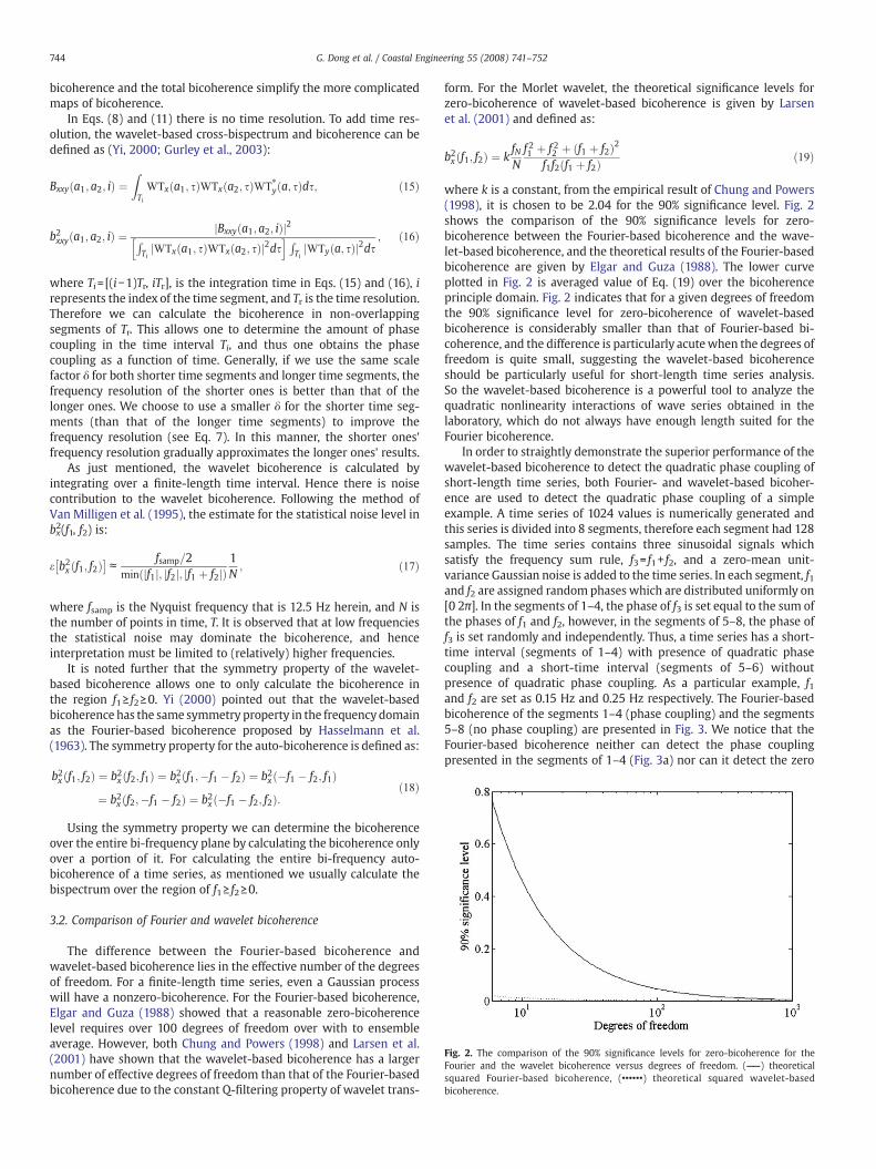
Fig. 2. The comparison of the 90% significance levels for zero-bicoherence for theFourier and the wavelet bicoherence versus degrees of freedom. (——) theoreticalsquared Fourier-based bicoherence, (••••••) theoretical squared wavelet-basedbicoherence.

744 G. Dong et al. / Coastal Engineering 55 (2008) 741–752

bicoherence and the total bicoherence simplify the more complicatedmaps of bicoherence.

In Eqs. (8) and (11) there is no time resolution. To add time res-olution, the wavelet-based cross-bispectrum and bicoherence can bedefined as (Yi, 2000; Gurley et al., 2003):

Bxxy a1; a2; ið Þ ¼ZTiWTx a1; sð ÞWTx a2; sð ÞWT⁎

y a; sð Þds; ð15Þ

b2xxy a1; a2; ið Þ ¼ jBxxy a1; a2; ið Þj2RTijWTx a1; sð ÞWTx a2; sð Þj2ds

h i RTijWTy a; sð Þj2ds

; ð16Þ

where Ti=[(i−1)Tr, iTr], is the integration time in Eqs. (15) and (16), irepresents the index of the time segment, and Tr is the time resolution.Therefore we can calculate the bicoherence in non-overlappingsegments of Tr. This allows one to determine the amount of phasecoupling in the time interval Ti, and thus one obtains the phasecoupling as a function of time. Generally, if we use the same scalefactor δ for both shorter time segments and longer time segments, thefrequency resolution of the shorter ones is better than that of thelonger ones. We choose to use a smaller δ for the shorter time seg-ments (than that of the longer time segments) to improve thefrequency resolution (see Eq. 7). In this manner, the shorter ones'frequency resolution gradually approximates the longer ones' results.

As just mentioned, the wavelet bicoherence is calculated byintegrating over a finite-length time interval. Hence there is noisecontribution to the wavelet bicoherence. Following the method ofVan Milligen et al. (1995), the estimate for the statistical noise level inbx2(f1, f2) is:

e b2x f1; f2ð Þ� �c

fsamp=2min jf1j; jf2j; jf1 þ f2jð Þ

1N; ð17Þ

where fsamp is the Nyquist frequency that is 12.5 Hz herein, and N isthe number of points in time, T. It is observed that at low frequenciesthe statistical noise may dominate the bicoherence, and henceinterpretation must be limited to (relatively) higher frequencies.

It is noted further that the symmetry property of the wavelet-based bicoherence allows one to only calculate the bicoherence inthe region f1≥ f2≥0. Yi (2000) pointed out that the wavelet-basedbicoherence has the same symmetry property in the frequency domainas the Fourier-based bicoherence proposed by Hasselmann et al.(1963). The symmetry property for the auto-bicoherence is defined as:

b2x f1; f2ð Þ ¼ b2x f2; f1ð Þ ¼ b2x f1;�f1 � f2ð Þ ¼ b2x �f1 � f2; f1ð Þ¼ b2x f2;�f1 � f2ð Þ ¼ b2x �f1 � f2; f2ð Þ:

ð18Þ

Using the symmetry property we can determine the bicoherenceover the entire bi-frequency plane by calculating the bicoherence onlyover a portion of it. For calculating the entire bi-frequency auto-bicoherence of a time series, as mentioned we usually calculate thebispectrum over the region of f1≥ f2≥0.

3.2. Comparison of Fourier and wavelet bicoherence

The difference between the Fourier-based bicoherence andwavelet-based bicoherence lies in the effective number of the degreesof freedom. For a finite-length time series, even a Gaussian processwill have a nonzero-bicoherence. For the Fourier-based bicoherence,Elgar and Guza (1988) showed that a reasonable zero-bicoherencelevel requires over 100 degrees of freedom over with to ensembleaverage. However, both Chung and Powers (1998) and Larsen et al.(2001) have shown that the wavelet-based bicoherence has a largernumber of effective degrees of freedom than that of the Fourier-basedbicoherence due to the constant Q-filtering property of wavelet trans-

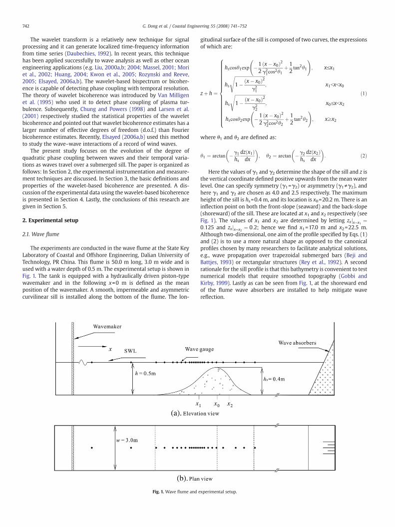
form. For the Morlet wavelet, the theoretical significance levels forzero-bicoherence of wavelet-based bicoherence is given by Larsenet al. (2001) and defined as:

b2x f1; f2ð Þ ¼ kfNNf 21 þ f 22 þ f1 þ f2ð Þ2

f1f2 f1 þ f2ð Þ ð19Þ

where k is a constant, from the empirical result of Chung and Powers(1998), it is chosen to be 2.04 for the 90% significance level. Fig. 2shows the comparison of the 90% significance levels for zero-bicoherence between the Fourier-based bicoherence and the wave-let-based bicoherence, and the theoretical results of the Fourier-basedbicoherence are given by Elgar and Guza (1988). The lower curveplotted in Fig. 2 is averaged value of Eq. (19) over the bicoherenceprinciple domain. Fig. 2 indicates that for a given degrees of freedomthe 90% significance level for zero-bicoherence of wavelet-basedbicoherence is considerably smaller than that of Fourier-based bi-coherence, and the difference is particularly acutewhen the degrees offreedom is quite small, suggesting the wavelet-based bicoherenceshould be particularly useful for short-length time series analysis.So the wavelet-based bicoherence is a powerful tool to analyze thequadratic nonlinearity interactions of wave series obtained in thelaboratory, which do not always have enough length suited for theFourier bicoherence.

In order to straightly demonstrate the superior performance of thewavelet-based bicoherence to detect the quadratic phase coupling ofshort-length time series, both Fourier- and wavelet-based bicoher-ence are used to detect the quadratic phase coupling of a simpleexample. A time series of 1024 values is numerically generated andthis series is divided into 8 segments, therefore each segment had 128samples. The time series contains three sinusoidal signals whichsatisfy the frequency sum rule, f3= f1+ f2, and a zero-mean unit-variance Gaussian noise is added to the time series. In each segment, f1and f2 are assigned random phases which are distributed uniformly on[0 2π]. In the segments of 1–4, the phase of f3 is set equal to the sum ofthe phases of f1 and f2, however, in the segments of 5–8, the phase off3 is set randomly and independently. Thus, a time series has a short-time interval (segments of 1–4) with presence of quadratic phasecoupling and a short-time interval (segments of 5–6) withoutpresence of quadratic phase coupling. As a particular example, f1and f2 are set as 0.15 Hz and 0.25 Hz respectively. The Fourier-basedbicoherence of the segments 1–4 (phase coupling) and the segments5–8 (no phase coupling) are presented in Fig. 3. We notice that theFourier-based bicoherence neither can detect the phase couplingpresented in the segments of 1–4 (Fig. 3a) nor can it detect the zero

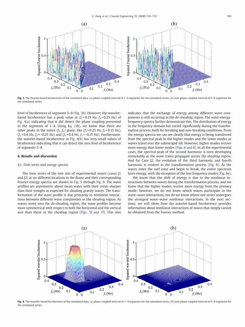
Fig. 3. The Fourier-based bicoherence of the simulated data. (a) phase coupled interval of 1–4 segments for the simulated series, (b) non-phase coupled interval of 5–8 segments forthe simulated series.

745G. Dong et al. / Coastal Engineering 55 (2008) 741–752

level of bicoherence of segments 5–8 (Fig. 3b). However, the wavelet-based bicoherence has a peak value at (f1=0.15 Hz, f2=0.25 Hz) ofFig. 4(a) indicating that it did detect the phase coupling presentedin the segments of 1–4. Using Eq. (18), we know that there areother peaks in the entire (f1, f2) plane, like (f1=0.25 Hz, f2=0.15 Hz),(f1=0.4 Hz, f2=−0.25 Hz) and (f1=0.4 Hz, f1=−0.15 Hz). Furthermore,the wavelet-based bicoherence in Fig. 4(b) has very small values ofbicoherence indicating that it can detect the zero level of bicoherenceof segments 5–8.

4. Results and discussion

4.1. Time series and energy spectra

The time series of the two sets of experimental waves (cases J1and J2) at six different locations in the flume and their correspondingFourier energy spectra are shown in Fig. 5 through Fig. 8. The waveprofiles are asymmetric about mean water with their crests sharperthan their troughs as expected for shoaling gravity waves. The trans-formation of the wave profile is due primarily to nonlinear interac-tions between different wave components in the shoaling region. Aswaves move into the de-shoaling region, the wave profiles becomemore symmetrical with respect to both the horizontal and the verticalaxis than those in the shoaling region (Figs. 5f and 7f). This also

Fig. 4. The wavelet-based bicoherence of the simulated data. (a) phase coupled interval of 1–the simulated series.

indicates that the exchange of energy among different wave com-ponents is still occurring in the de-shoaling region. The wave energy-frequency spectra further demonstrate this. The distribution of energyin the frequency domain has varied significantly during the transfor-mation process, both for breaking and non-breaking conditions. Fromthe energy spectra we can see clearly that energy is being transferredfrom the spectral peak to the higher modes and the lower modes aswaves travel over the submerged sill. However, higher modes receivemore energy than lower modes (Figs. 6 and 8). In all the experimentalcases, the spectral peak of the second harmonic is seen developingremarkably as the wave trains propagate across the shoaling region.And for Case J2, the evolution of the third harmonic and fourthharmonic is evident in the transformation process (Fig. 8). As thewaves enter the surf zone and begin to break, the entire spectrumloses energy, with the exception of the low frequency modes (Fig. 8e).

We know that the shift of energy is due to the nonlinear in-teractions between waves during the transformation process, and weknow that the higher modes receive more energy from the primarymode; however, we do not know which waves participate in thewave–wave interactions, nor do we knowwhere one series undergoesthe strongest wave–wave nonlinear interactions. In the next sec-tions, we will show how the wavelet-based bicoherence providesinformation about nonlinear interactions of waves that simply cannotbe obtained from the Fourier method.

4 segments for the simulated series, (b) non-phase coupled interval of 5–8 segments for

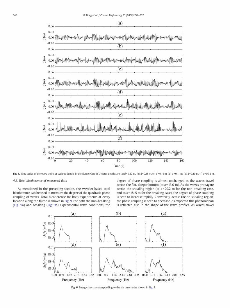
Fig. 5. Time series of the wave trains at various depths in the flume (Case J1). Water depths are (a) d=0.32 m, (b) d=0.18 m, (c) d=0.14 m, (d) d=0.11 m, (e) d=0.10 m, (f) d=0.32 m.

746 G. Dong et al. / Coastal Engineering 55 (2008) 741–752

4.2. Total bicoherence of measured data

As mentioned in the preceding section, the wavelet-based totalbicoherence can be used to measure the degree of the quadratic phasecoupling of waves. Total bicoherence for both experiments at everylocation along the flume is shown in Fig. 9. For both the non-breaking(Fig. 9a) and breaking (Fig. 9b) experimental wave conditions, the

Fig. 6. Energy spectra corresponding to

degree of phase coupling is almost unchanged as the waves travelacross the flat, deeper bottom (to x=13.0 m). As the waves propagateacross the shoaling region (to x=20.2 m for the non-breaking case,and to x=18. 5 m for the breaking case), the degree of phase couplingis seen to increase rapidly. Conversely, across the de-shoaling region,the phase coupling is seen to decrease. As expected this phenomenonis reflected also in the shape of the wave profiles. As waves travel

the six time series shown in Fig. 5.

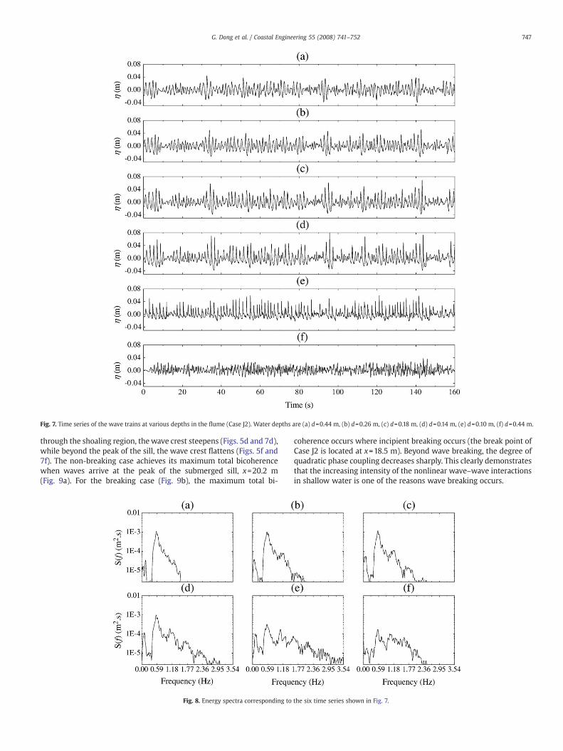
Fig. 7. Time series of the wave trains at various depths in the flume (Case J2). Water depths are (a) d=0.44 m, (b) d=0.26 m, (c) d=0.18 m, (d) d=0.14 m, (e) d=0.10 m, (f) d=0.44 m.

747G. Dong et al. / Coastal Engineering 55 (2008) 741–752

through the shoaling region, the wave crest steepens (Figs. 5d and 7d),while beyond the peak of the sill, the wave crest flattens (Figs. 5f and7f). The non-breaking case achieves its maximum total bicoherencewhen waves arrive at the peak of the submerged sill, x=20.2 m(Fig. 9a). For the breaking case (Fig. 9b), the maximum total bi-

Fig. 8. Energy spectra corresponding to

coherence occurs where incipient breaking occurs (the break point ofCase J2 is located at x=18.5 m). Beyond wave breaking, the degree ofquadratic phase coupling decreases sharply. This clearly demonstratesthat the increasing intensity of the nonlinear wave–wave interactionsin shallow water is one of the reasons wave breaking occurs.

the six time series shown in Fig. 7.

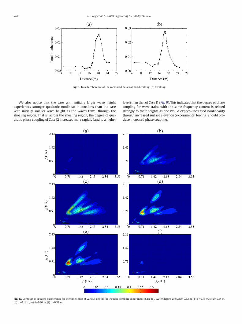
Fig. 9. Total bicoherence of the measured data: (a) non-breaking, (b) breaking.

748 G. Dong et al. / Coastal Engineering 55 (2008) 741–752

We also notice that the case with initially larger wave heightexperiences stronger quadratic nonlinear interactions than the casewith initially smaller wave height as the waves travel through theshoaling region. That is, across the shoaling region, the degree of qua-dratic phase coupling of Case J2 increases more rapidly (and to a higher

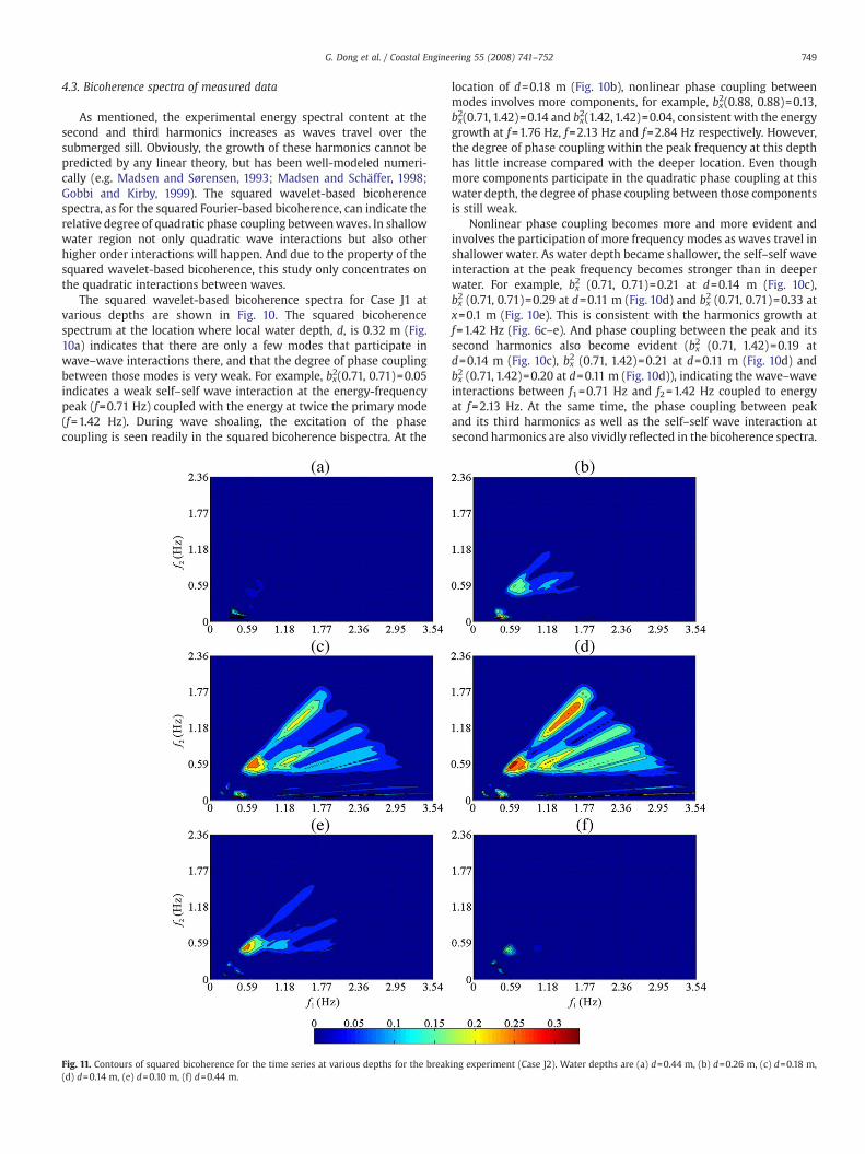
Fig. 10. Contours of squared bicoherence for the time series at various depths for the non-bre(d) d=0.11 m, (e) d=0.10 m, (f) d=0.32 m.

level) than that of Case J1 (Fig. 9). This indicates that the degree of phasecoupling for wave trains with the same frequency content is relatedstrongly to their heights as one would expect—increased nonlinearitythrough increased surface elevation (experimental forcing) should pro-duce increased phase coupling.

aking experiment (Case J1). Water depths are (a) d=0.32 m, (b) d=0.18 m, (c) d=0.14 m,

749G. Dong et al. / Coastal Engineering 55 (2008) 741–752

4.3. Bicoherence spectra of measured data

As mentioned, the experimental energy spectral content at thesecond and third harmonics increases as waves travel over thesubmerged sill. Obviously, the growth of these harmonics cannot bepredicted by any linear theory, but has been well-modeled numeri-cally (e.g. Madsen and Sørensen, 1993; Madsen and Schäffer, 1998;Gobbi and Kirby, 1999). The squared wavelet-based bicoherencespectra, as for the squared Fourier-based bicoherence, can indicate therelative degree of quadratic phase coupling betweenwaves. In shallowwater region not only quadratic wave interactions but also otherhigher order interactions will happen. And due to the property of thesquared wavelet-based bicoherence, this study only concentrates onthe quadratic interactions between waves.

The squared wavelet-based bicoherence spectra for Case J1 atvarious depths are shown in Fig. 10. The squared bicoherencespectrum at the location where local water depth, d, is 0.32 m (Fig.10a) indicates that there are only a few modes that participate inwave–wave interactions there, and that the degree of phase couplingbetween those modes is very weak. For example, bx2(0.71, 0.71)=0.05indicates a weak self–self wave interaction at the energy-frequencypeak (f=0.71 Hz) coupled with the energy at twice the primary mode(f=1.42 Hz). During wave shoaling, the excitation of the phasecoupling is seen readily in the squared bicoherence bispectra. At the

Fig. 11. Contours of squared bicoherence for the time series at various depths for the break(d) d=0.14 m, (e) d=0.10 m, (f) d=0.44 m.

location of d=0.18 m (Fig. 10b), nonlinear phase coupling betweenmodes involves more components, for example, bx2(0.88, 0.88)=0.13,bx2(0.71, 1.42)=0.14 and bx

2(1.42, 1.42)=0.04, consistent with the energygrowth at f=1.76 Hz, f=2.13 Hz and f=2.84 Hz respectively. However,the degree of phase coupling within the peak frequency at this depthhas little increase compared with the deeper location. Even thoughmore components participate in the quadratic phase coupling at thiswater depth, the degree of phase coupling between those componentsis still weak.

Nonlinear phase coupling becomes more and more evident andinvolves the participation of more frequency modes as waves travel inshallower water. As water depth became shallower, the self–self waveinteraction at the peak frequency becomes stronger than in deeperwater. For example, bx

2 (0.71, 0.71)=0.21 at d=0.14 m (Fig. 10c),bx2 (0.71, 0.71)=0.29 at d=0.11 m (Fig. 10d) and bx

2 (0.71, 0.71)=0.33 atx=0.1 m (Fig. 10e). This is consistent with the harmonics growth atf=1.42 Hz (Fig. 6c–e). And phase coupling between the peak and itssecond harmonics also become evident (bx2 (0.71, 1.42)=0.19 atd=0.14 m (Fig. 10c), bx2 (0.71, 1.42)=0.21 at d=0.11 m (Fig. 10d) andbx2 (0.71, 1.42)=0.20 at d=0.11 m (Fig. 10d)), indicating the wave–wave

interactions between f1=0.71 Hz and f2=1.42 Hz coupled to energyat f=2.13 Hz. At the same time, the phase coupling between peakand its third harmonics as well as the self–self wave interaction atsecond harmonics are also vividly reflected in the bicoherence spectra.

ing experiment (Case J2). Water depths are (a) d=0.44 m, (b) d=0.26 m, (c) d=0.18 m,

750 G. Dong et al. / Coastal Engineering 55 (2008) 741–752

Besides of phase coupling within the peak, between the peak and itshigher harmonics and between the higher harmonics themselves,there are other modes participating in the quadratic nonlinearprocess. For example, bx

2 (0.58, 1.70)=0.11 at depth 0.1(Fig. 10e),indicates the wave–wave interactions between f1=0.58 Hz andf2=1.70 Hz coupled to energy at f=2.28 Hz. In the de-shoaling region(Fig. 10f), the squared bicoherence spectrum indicates that the rangeof modes participating in the nonlinear interaction is reduced, andonly the weak phase coupling within the peak frequency exists at thislocation (bx2 (0.71, 0.71)=0.11), mainly due to the release of thebounded higher harmonics and the increase of the water depth afterwaves travel over the top of the sill.

The bicoherence spectra of Case J2 at six different locations areshown in Fig. 11. From this set of figures we see that the nonlinearphase coupling for Case J2 has similar characteristics to that of Case J1.The quadratic phase coupling is very weak as the wave trains travelover deeper bottom (Fig. 11a), but becomes more and more evident,and involves the participation of more frequency modes as the wavestravel across the shoaling region. The self–self wave interaction atthe peak frequency (0.59 Hz) becomes more and more stronger aswaves shoaling. As water depth becomes shallower, quadratic phasecoupling spreads not only to encompass interactions between thepeak frequency and its higher harmonics, but also to interactionsbetween those higher harmonics themselves. For example, bx2 (0.59,1.18)=0.23, bx2 (0.59, 1.77)=0.15 and bx

2 (1.18, 1.18)=0.17 at d=0.18 m(Fig. 11c); bx2 (0.59, 1.18)=0.27, bx2 (0.59, 1.77)=0.21 and bx

2 (1.18, 1.18)=0.25 at d=0.14 m (Fig. 11d). This is consistent with the energytransfer to the frequencies at f=1.77 Hz and f=2.36 Hz (Fig. 7). Theprimary difference between Case J1 and Case J2 is that the maximumdegree of phase coupling for Case J1 occurs at the top of the sill(x=20.2 m) whereas for Case J2 it happens at incipient breaking(x=18.5 m). After wave breaking, the modes participate in the qua-dratic phase coupling decrease and the intensity of the nonlinearcoupling betweenmodes becomes weaker than that of before breaking,for the wave heights decrease and the bound higher harmonics arereleased after breaking.

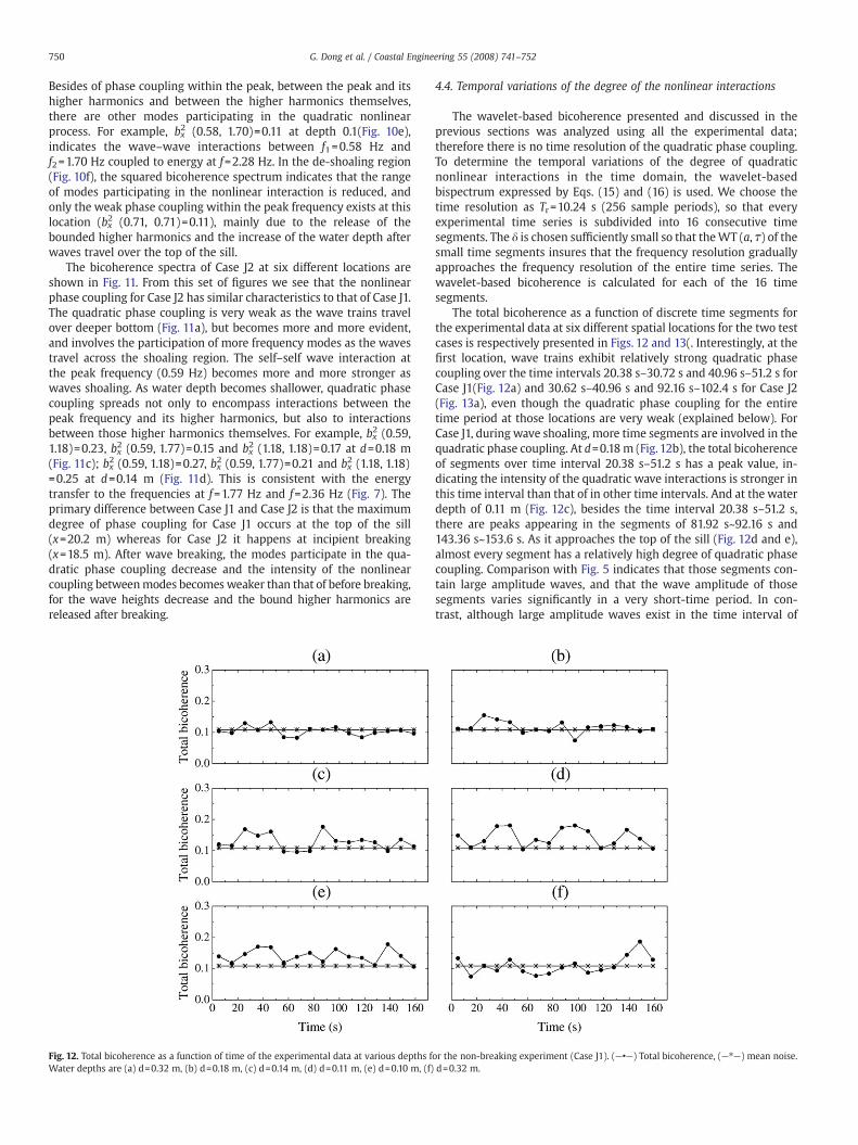
Fig. 12. Total bicoherence as a function of time of the experimental data at various depths fWater depths are (a) d=0.32 m, (b) d=0.18 m, (c) d=0.14 m, (d) d=0.11 m, (e) d=0.10 m, (f)

4.4. Temporal variations of the degree of the nonlinear interactions

The wavelet-based bicoherence presented and discussed in theprevious sections was analyzed using all the experimental data;therefore there is no time resolution of the quadratic phase coupling.To determine the temporal variations of the degree of quadraticnonlinear interactions in the time domain, the wavelet-basedbispectrum expressed by Eqs. (15) and (16) is used. We choose thetime resolution as Tr=10.24 s (256 sample periods), so that everyexperimental time series is subdivided into 16 consecutive timesegments. The δ is chosen sufficiently small so that theWT (a, τ) of thesmall time segments insures that the frequency resolution graduallyapproaches the frequency resolution of the entire time series. Thewavelet-based bicoherence is calculated for each of the 16 timesegments.

The total bicoherence as a function of discrete time segments forthe experimental data at six different spatial locations for the two testcases is respectively presented in Figs. 12 and 13(. Interestingly, at thefirst location, wave trains exhibit relatively strong quadratic phasecoupling over the time intervals 20.38 s–30.72 s and 40.96 s–51.2 s forCase J1(Fig. 12a) and 30.62 s–40.96 s and 92.16 s–102.4 s for Case J2(Fig. 13a), even though the quadratic phase coupling for the entiretime period at those locations are very weak (explained below). ForCase J1, during wave shoaling, more time segments are involved in thequadratic phase coupling. At d=0.18m (Fig. 12b), the total bicoherenceof segments over time interval 20.38 s–51.2 s has a peak value, in-dicating the intensity of the quadratic wave interactions is stronger inthis time interval than that of in other time intervals. And at the waterdepth of 0.11 m (Fig. 12c), besides the time interval 20.38 s–51.2 s,there are peaks appearing in the segments of 81.92 s~92.16 s and143.36 s~153.6 s. As it approaches the top of the sill (Fig. 12d and e),almost every segment has a relatively high degree of quadratic phasecoupling. Comparison with Fig. 5 indicates that those segments con-tain large amplitude waves, and that the wave amplitude of thosesegments varies significantly in a very short-time period. In con-trast, although large amplitude waves exist in the time interval of

or the non-breaking experiment (Case J1). (—•—) Total bicoherence, (—⁎—) mean noise.d=0.32 m.

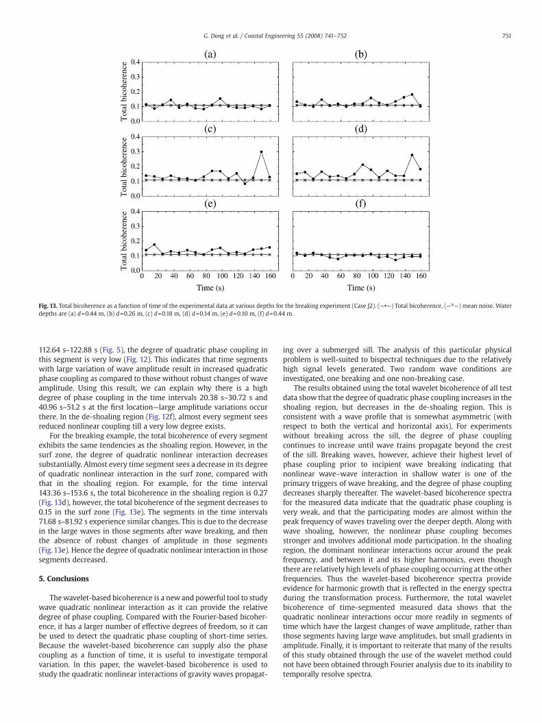
Fig. 13. Total bicoherence as a function of time of the experimental data at various depths for the breaking experiment (Case J2). (—•—) Total bicoherence, (—⁎—) mean noise. Waterdepths are (a) d=0.44 m, (b) d=0.26 m, (c) d=0.18 m, (d) d=0.14 m, (e) d=0.10 m, (f) d=0.44 m.

751G. Dong et al. / Coastal Engineering 55 (2008) 741–752

112.64 s~122.88 s (Fig. 5), the degree of quadratic phase coupling inthis segment is very low (Fig. 12). This indicates that time segmentswith large variation of wave amplitude result in increased quadraticphase coupling as compared to those without robust changes of waveamplitude. Using this result, we can explain why there is a highdegree of phase coupling in the time intervals 20.38 s–30.72 s and40.96 s–51.2 s at the first location—large amplitude variations occurthere. In the de-shoaling region (Fig. 12f), almost every segment seesreduced nonlinear coupling till a very low degree exists.

For the breaking example, the total bicoherence of every segmentexhibits the same tendencies as the shoaling region. However, in thesurf zone, the degree of quadratic nonlinear interaction decreasessubstantially. Almost every time segment sees a decrease in its degreeof quadratic nonlinear interaction in the surf zone, compared withthat in the shoaling region. For example, for the time interval143.36 s~153.6 s, the total bicoherence in the shoaling region is 0.27(Fig. 13d), however, the total bicoherence of the segment decreases to0.15 in the surf zone (Fig. 13e). The segments in the time intervals71.68 s~81.92 s experience similar changes. This is due to the decreasein the large waves in those segments after wave breaking, and thenthe absence of robust changes of amplitude in those segments(Fig. 13e). Hence the degree of quadratic nonlinear interaction in thosesegments decreased.

5. Conclusions

Thewavelet-based bicoherence is a new and powerful tool to studywave quadratic nonlinear interaction as it can provide the relativedegree of phase coupling. Compared with the Fourier-based bicoher-ence, it has a larger number of effective degrees of freedom, so it canbe used to detect the quadratic phase coupling of short-time series.Because the wavelet-based bicoherence can supply also the phasecoupling as a function of time, it is useful to investigate temporalvariation. In this paper, the wavelet-based bicoherence is used tostudy the quadratic nonlinear interactions of gravity waves propagat-

ing over a submerged sill. The analysis of this particular physicalproblem is well-suited to bispectral techniques due to the relativelyhigh signal levels generated. Two random wave conditions areinvestigated, one breaking and one non-breaking case.

The results obtained using the total wavelet bicoherence of all testdata show that the degree of quadratic phase coupling increases in theshoaling region, but decreases in the de-shoaling region. This isconsistent with a wave profile that is somewhat asymmetric (withrespect to both the vertical and horizontal axis). For experimentswithout breaking across the sill, the degree of phase couplingcontinues to increase until wave trains propagate beyond the crestof the sill. Breaking waves, however, achieve their highest level ofphase coupling prior to incipient wave breaking indicating thatnonlinear wave–wave interaction in shallow water is one of theprimary triggers of wave breaking, and the degree of phase couplingdecreases sharply thereafter. The wavelet-based bicoherence spectrafor the measured data indicate that the quadratic phase coupling isvery weak, and that the participating modes are almost within thepeak frequency of waves traveling over the deeper depth. Along withwave shoaling, however, the nonlinear phase coupling becomesstronger and involves additional mode participation. In the shoalingregion, the dominant nonlinear interactions occur around the peakfrequency, and between it and its higher harmonics, even thoughthere are relatively high levels of phase coupling occurring at the otherfrequencies. Thus the wavelet-based bicoherence spectra provideevidence for harmonic growth that is reflected in the energy spectraduring the transformation process. Furthermore, the total waveletbicoherence of time-segmented measured data shows that thequadratic nonlinear interactions occur more readily in segments oftime which have the largest changes of wave amplitude, rather thanthose segments having large wave amplitudes, but small gradients inamplitude. Finally, it is important to reiterate that many of the resultsof this study obtained through the use of the wavelet method couldnot have been obtained through Fourier analysis due to its inability totemporally resolve spectra.

752 G. Dong et al. / Coastal Engineering 55 (2008) 741–752

Acknowledgments

This research is supported financially by the National NaturalScience Foundation (50679010), Program for New Century ExcellentTalents in Universities of China (NCET-04-0267), and Program forChangjiang Scholars and Innovative Research Teams of Colleges andUniversities of China (IRT0420).

References

Beji, S., Battjes, J.A., 1993. Experimental investigation of wave propagation over a bar.Coastal Engineering 19, 151–162.

Chung, J., Powers, J., 1998. The statistics of wavelet-based bicoherence. Proceedings ofthe IEEE-SP International Symposium on Time-Frequency and Time-Scale Analysis.Pittsburgh, Pennsylvania, USA, pp. 141–144.

Daubechies, I., 1992. Ten Lectures on Wavelets. Society for Industrial & Applied Mathe-matics, Philadelphia, PA.

Elgar, S., Guza, R.T., 1985. Observations of bispectra of shoaling surface gravity waves.Journal of Fluid Mechanics 161, 425–448.

Elgar, S., Guza, R.T., 1988. Statistics of bicoherence. IEEE Transactions on Acoustics,Speech, and Signal Processing 36, 1667–1668.

Elgar, S., Freilich, M., Guza, R.T., 1990. Model-data comparisons of moments of non-breaking shoaling surface gravity waves. Journal of Geophysical Research 95 (C9),16055–16063.

Elgar, S., Guza, R.T., Freilich, M., 1993. Observations of nonlinear interactions in direc-tionally spread shoaling surface gravity waves. Journal of Geophysical Research 98(C11), 20299–20305.

Elsayed, M.A.K., 2006a. A novel technique in analyzing non-linear wave–wave inter-action. Ocean Engineering 33, 168–180.

Elsayed, M.A.K., 2006b. Wavelet bicoherence analysis of wind–wave interaction. OceanEngineering 33, 458–470.

Farge, M., 1992. Wavelet transforms and their applications to turbulence. AnnualReview of Fluid Mechanics 24, 395–457.

Gobbi, M.F., Kirby, J.T., 1999. Wave evolution over submerged sills: tests of a high-orderBoussinesq model. Coastal Engineering 37, 57–96.

Goda, Y., 1985. Random Seas and Design of Maritime Structures. Columbia UniversityPress, New York.

Gurley, K., Kijewski, T., Kareem, A., 2003. First- and higher-order correlation detectionusing wavelet transforms. Journal of Engineering Mechanics 129, 188–201.

Hasselmann, K., 1962. On the non-linear energy transfer in a gravity-wave spectrum,Part I. General theory. Journal of Fluid Mechanics 12, 481–500.

Hasselmann, K.,Munk,W.,MacDonald, G.,1963. Bispectra of oceanwaves. In: Rosenblatt,M. (Ed.), Time Series Analysis. Wiley, New York, pp. 125–139.

Huang,M.C., 2004.Waveparameters and functions inwavelet analysis. Ocean Engineering31, 111–125.

Kwon, S.H., Lee, H.S., Kim, C.H., 2005. Wavelet transform based coherence analysis offreak wave and its impact. Ocean Engineering 32, 1572–1589.

Larsen, Y., Hanssen, A., Pecseli, H.L., 2001. Analysis of non-stationary mode coupling bymeans of wavelet-bicoherence. IEEE International Conference on Acoustics, Speech,and Signal Processing. Salt Lake City, Utah, USA, pp. 3581–3584.

Liu, P.C., 2000a. Is the wind wave frequency spectrum outdated? Ocean Engineering 27,577–588.

Liu, P.C., 2000b. Wave grouping characteristics in nearshore Great Lakes. OceanEngineering 27, 1221–1230.

Liu, P.C., 2004. A discrete wavelet analysis of freakwaves in the ocean. Journal of AppliedMathematics 5, 379–394.

Longuet-Higgins, M.S., Stewart, R.W., 1962. Radiation stress and mass transport ingravity waves, with application to surf-beats. Journal of Fluid Mechanics 13,481–504.

Madsen, P.A., Sørensen, O.R., 1993. Bound waves and triad interactions in shallowwater.Ocean Engineering 20, 259–388.

Madsen, P.A., Schäffer, H.A., 1998. Higher-order Boussinesq-type equations for surfacegravity waves: derivation and analysis. Philosophical Transactions of the RoyalSociety of London A356, 3123–3184.

Massel, S.R., 2001. Wavelet analysis for processing of ocean surface wave records. OceanEngineering 28, 957–987.

Mori, N., Liu, P.C., Yasuda, T., 2002. Analysis of freak wave measurements in the Sea ofJapan. Ocean Engineering 29, 1399–1414.

Phillips, O.M., 1977. The Dynamics of the Upper Ocean. Cambridge University Press,New York.

Rey, V., Belrous, M., Guaselli, E., 1992. Propagation of surface gravity waves over arectangular submerged bar. Journal of Fluid Mechanics 9, 193–217.

Rozynski, G., Reeve, D., 2005. Multi-resolution analysis of nearshore hydrodynamicsusing discrete wavelet transforms. Coastal Engineering 52, 771–792.

Schäffer, H.A., 1996. Second-order wavemaker theory for irregular waves. OceanEngineering 23, 47–88.

Torrence, C., Compo, G.P., 1998. A practical guide to wavelet analysis. Bulletin of AmericanMeteorology Society 79 (1), 61–78.

Van Milligen, B.P., Sánchez, E., Estrada, T., Hidalgo, C., Brañas, B., Carreras, B., García, L.,1995.Wavelet bicoherence: a new turbulence analysis tool. Physics of Plasmas 2 (8),3017–3032.

Yi, E.J., 2000. Applications of Wavelets to Nonlinear Wave Analysis and Digital Com-munication. Ph.D. thesis. The University of Texas at Austin, USA.

Young, I.R., Eldeberky, Y., 1998. Observations of triad coupling of finite depth windwaves. Coastal Engineering 33, 137–154.

Guohai DongProfessorState Key Laboratory of Coastal and Offshore Engineering, Dalian University ofTechnologyE-mail: ghdong@dlut.edu.cnB.S. Dalian University of Technology, 1986; Naval ArchitectureM.C.E. Dalian University of Technology, 1989; Coastal EngineeringPh.D. Dalian University of Technology, 1992; Coastal Engineering

Yuxiang MaPh.D. CandidateState Key Laboratory of Coastal and Offshore Engineering, Dalian University ofTechnologyE-mail: yuxma@126.comB.S. University of South China, 2004; Civil Engineering

Marc PerlinProfessorDepartment of Naval Architecture and Marine Engineering, University of MichiganE-mail: perlin@umich.eduB.S. Drexel University, 1974; Civil EngineeringM.C.E. University of Delaware, 1978; Civil EngineeringPh.D. University of Florida, 1989; Engineering Mechanics

Xiaozhou MaPostal DoctorState Key Laboratory of Coastal and Offshore Engineering, Dalian University ofTechnologyE-mail: maxzh@dlut.edu.cnB.S. China Three Gorges University, 2000; Civil EngineeringPh.D. Dalian University of Technology, 2006; Coastal Engineering

Bo YuPh.D. CandidateState Key Laboratory of Coastal and Offshore Engineering, Dalian University ofTechnologyE-mail: handsomyuyu@hotmail.comB.S. Dalian University of Technology, 2004; Harbor, waterway and Coastal Engineering

Jianwu XuM.C.E. CandidateState Key Laboratory of Coastal and Offshore Engineering, Dalian University ofTechnologyE-mail: xjw0432@163.comB.S. Hohai University, 2005; Harbor, Waterway and Coastal Engineering