Embed Size (px)
DESCRIPTION
Thermoacoustic engine is one of the emerging technologies in the field of energy conversion. Thermoacoustic engines convert thermal energy, possibly at relatively low temperatures to mechanical energy in the form of acoustic oscillations of high amplitudes that can drive a thermoacoustic refrigerator or can be converted to electrical energy using a linear alternator. In this work, a prototype of a thermoacoustic engine was built, operated and tested. Sustainable operation of the engine is possible due to the relatively efficient hot and cold heat exchangers that were able to sustain the temperature gradient across the stack.Both the transient and steady-state performance of the thermoacoustic engine are investigated using variable gas mixtures and using square-cell stacks of variable porosities. The engine performance is studied during full runs consisting of start-up, steady operation, and shutting-down. The steady-state engine performance and wave characteristics are investigated at different heat input values, different gas mixtures, and different stack porosities. Inserts with different patterns and open areas are used inside the resonator to investigate their effect on suppressing the high harmonics of the produced acoustic wave. A numerical model of the current prototype is built using the free simulation software DELTAEC. The model is validated using the experimental data and is then used to obtain more information about the engine performance. Results show that the used gas mixture, the pressure ratio, and the stack cell dimensions significantly affect the engine power output, the wave dynamic pressure amplitude, and the harmonic content of the wave. Experimental data agrees with DELTAEC calculations in trend, but the values of acoustic power and dynamic pressure are significantly lower than the numerical model calculations. The values of the frequency are within 3% of the measured values. The transient analysis shows that the dynamic pressure amplitude of the gas reaches a peak after onset and then decreases to a steady value during the run. The onset temperature of the engine is always higher than the temperature at which the system stops producing oscillations while shut-down. The hysteresis characteristics is significantly affected by the thermal conductivity of the gas mixture, the stack cell dimensions, the mean temperature at starting, and the time of the cycle. The heat exchange process at the cold side is enhanced by the existence of the wave.In this work, several inserts of different thicknesses, open area, positions, and hole patterns are inserted into the resonator to suppress the harmonics. All inserts caused lower harmonic content with respect to the case with no inserts. Inserts of low open area cause the performance to degrade and produce low acoustic powers. Inserts with higher thickness gave better performance. Amongst all inserts used, the highest acoustic power is obtained using an insert with an open area of 50% of the resonator area, a pattern of several distributed holes, a thickness of 3 cm, and at a position of 0.33 of the fundamental wavelength measured from the cold-side blind flange.
Citation preview

EXPERIMENTAL INVESTIGATIONS ON A
STANDING-WAVE THERMOACOUSTIC ENGINE
By
Mahmoud Mohamed Emam
A Thesis Submitted to the Faculty of Engineering
at Cairo University in Partial Fulfillment of the
Requirements for the Degree of
MASTER OF SCIENCE
In
MECHANICAL POWER ENGINEERING
FACULTY OF ENGINEERING, CAIRO UNIVERSITY
GIZA, EGYPT
2013

II
EXPERIMENTAL INVESTIGATIONS ON A
STANDING-WAVE THERMOACOUSTIC ENGINE
By
Mahmoud Mohamed Emam
In
MECHANICAL POWER ENGINEERING
Under Supervision of
FACULTY OF ENGINEERING, CAIRO UNIVERSITY
GIZA, EGYPT
2013
Prof. Dr. Mahmoud A. Fouad
Professor of Mechanical Power
Mechanical Power Engineering Department,
Faculty of Engineering, Cairo University
A Thesis Submitted to the Faculty of
Engineering at Cairo University in Partial
Fulfillment of the Requirements for the
Degree of
MASTER OF SCIENCE
Dr. Ehab Abdel-Rahman
Associate Professor of Physics
School of Sciences and Engineering
American University in Cairo
Dr. Abdelmaged H. Ibrahim Essawey
Assistant Professor, Mechanical Power
Engineering Department,
Faculty of Engineering, Cairo University

IV
Engineer’s Name: Mahmoud Mohamed Emam
Date of Birth: 01/01/1989
Nationality: Egyptian
E-mail: [email protected]
Phone: +2 011 1123 8133
Address: 16 Ard El-kamb, Elkanater
Elkhairia, Qalubia, Egypt
Registration Date: 01/10 /2010
Awarding Date: / /
Degree: Master of Science
Department: Mechanical Power Engineering
Supervisors:
Prof. Mahmoud Ahmed Fouad
Dr. Ehab Abdel-Rahman
Dr. Abdelmaged H. Ibrahim Essawy
Examiners:
Prof. Mahmoud A. El-Kady (External Examiner)
Prof. Essam E. Khalil (Internal Examiner)
Prof. Mahmoud A. Fouad (Main Advisor)
Thesis Title:
Experimental Investigations on A Standing-Wave Thermoacoustic
Engine
Key Words:
Thermoacoustic; Engine; Hysteresis; Acoustic; Harmonics
Summary:
In this work, both the transient and steady-state performance of the
thermoacoustic engine are investigated using variable gas mixtures and using
square-cell stacks of variable porosities. Transient engine performance is
studied during full runs consisting of start-up, steady operation, and shutting-
down. The steady-state engine performance and wave characteristics are
investigated at variable steady heat input values using different gas mixtures
and stack porosities. Inserts with different patterns and open areas are used
inside the resonator to investigate their effect on suppressing the high harmonics
of the produced acoustic wave. Results are compared with numerical simulation
carried out using the free simulation software DELTAEC.

V
Acknowledgements
So many people provided help and support throughout the course of this work. I
am particularly grateful towards my advisors, Professor Dr. Mahmoud A.
Fouad, Professor Dr. Ehab Abdul-Rahman, and Dr. Abdelmaged H. Ibrahim, for
their continuous help, guidance, support, and understanding in every step of this
work. I believe that their philosophy and friendship bring out the best in all of
their students and make a deep and lasting impression on their lives. Their broad
knowledge and constant encouragement are very much appreciated. The highly
appreciated understanding and support by Prof. Dr. Fouad is critical for me, not
only in this work, but along my entire academic life. The friendship of Dr.
Abdelmaged Ibrahim towards me and my family is something for which I am
especially grateful. I am very thankful to Professor Ehab Abdul-Rahman who
has been a wonderful source of advice and encouragement throughout my
graduate career. I acquired great knowledge from all the discussions I had with
him. I am very thankful to his continuous support and encouragement. Special
thanks to Professor Essam Khalil for his valuable help and discussions during
the early stages in preparing this work. His support and encouragement are
much appreciated. The support from my colleagues at the thermoacoustic lab in
AUC was essential. I would specially like to thank the efforts of the engineers
in the thermoacoustic research team in AUC. I have to thank the twin engineers
Ahmed and Khaled El-Beltagy for their efforts to help in producing this work.
Special thanks to engineers Micheal Rezk and Tarek Nigim for their continuous
help during various parts of this work.
The experimental procedures of this work were done in the labs of the physics
department in the American University in Cairo. The results were obtained
using the experimental apparatus in the labs of Youssef Jameel Science and
Technology Research Center. Special thanks to the thermoacoustic research
team in the American University in Cairo for their help and support.
I am very thankful to my family members: My mother, my sisters, and my
father for their love, support and prayers. The support and sacrifices made by
my family before and during this work are priceless.

VI
Table of Contents
Acknowledgements V
Table of contents VI
List of figures VIII
List of tables XI
Abstract XII
1. Introduction 1
1.1 Thermoacoustics 1
1.2 Historical review of thermoacoustics 3
1.3 Linear theory of thermoacoustics 4
1.3.1 Thermoacoustic phenomena 4
1.3.2 Thermodynamic cycle 4
1.3.3 Acoustic Background 8
1.3.4 General Thermoacoustic theory 10
1.4 Standing-wave Thermoacoustic Engine 15
1.5 Applications 16
1.6 Thesis Scope 17
2. Review of Related Literature 18
2.1 Historical background of thermoacoustic engines 18
2.2 Performance of standing-wave thermoacoustic engines 18
2.2.1 Experimental investigations on thermoacoustic engines 19
2.2.2 Numerical studies on thermoacoustic engines 20
2.2.3 Nonlinear effects 23
2.3 Applications 25
2.4 scope of the present study 26
3. Experimental Setup and Procedure 27
3.1 Standing wave thermoacoustic engine 27
3.1.1 Resonator 27
3.1.2 Thermoacoustic Stack 28
3.1.3 Heat exchangers 29
3.1.4 Working gas 30
3.1.5 Harmonic suppression inserts 31
3.2 Measurement system 33
3.2.1 Pressure measurements 33
3.2.2 Temperature Measurements 34

VII
3.3 Measurement Procedure 35
3.4 Data analysis 35
3.4.1 Onset temperature 35
3.4.2 Acoustic power 36
3.4.3 First and second law efficiencies 37
3.4.4 Harmonic content and frequency calculation 38
3.5 DELTAEC model 39
4. 4. Results and Discussion 41
4.1 Stable engine performance 41
4.1.1 Wave characteristics 41
4.1.2 Acoustic power output 43
4.1.3 Dynamic pressure amplitude 44
4.1.4 Frequency 45
4.2 Sustainability of operation 45
4.3 Transient operation and hysteresis 48
4.3.1 Hysteresis characteristics for cycles of different running times 48
4.3.2 Hysteresis characteristics for cycles of different starting conditions 49
4.3.3 Hysteresis in onset temperature 50
4.3.4 Hysteresis characteristics for different gas mixtures 52
4.3.5 Hysteresis characteristics for different pore sizes 53
4.3.6 Wave characteristics during a full run 55
4.4 Steady state operation using different gases and gas mixtures 57
4.4.1 Effect of gas mixture composition on output acoustic power 59
4.4.2 Effect of gas mixture composition on pressure amplitudes. 60
4.4.3 Effect of gas mixture composition on harmonic distortion 62
4.5 Harmonic suppression 65
4.5.1 Inserts effect on power and wave components 65
4.5.2 Effect of insert position 69
5. Conclusions and Suggestions for Future Work 71
5.1 Introduction 71
5.2 Conclusions of the present work 71
5.3 Recommendations 72
References 73
Appendix A: Properties of working gas mixture 77
Appendix B: DELTAEC code 78

VIII
List of Figures
Figure 1.1: Typical cycle of (a) thermoacoustic heat pump and (b) thermoacoustic prime mover. 5
Figure 1.2: P-V diagrams for the thermodynamic processes of the gas parcels as the distance from
the wall, d, increases. 6
Figure 1.3: Wave characteristics for a typical sinusoidal wave 8
Figure 1.4: A standing wave in a column full of air. 10
Figure 1.5: Geometry of the simplified parallel plate stacks. 10
Figure 1.6: Imaginary and real parts of the Rott function fk as function of the ratio of the hydraulic
radius and the thermal penetration depth. Three geometries are considered. For pin arrays, an internal
radius ri = 3δk is used in the calculations. 14
Figure 2.1: Square of pressure wave amplitude versus heat input to the standing-wave engine by
Chen and Garrett(14)
. 20
Figure 2.2: Square of end pressure amplitude versus input heat for different Helium mean pressures.
Lines are calculations and points are measurements. 21
Figure 2.3: Acoustic power flowing through the resonator in terms of the acoustic power dissipated
in an acoustic load. Symbols are measurements and the solid line is DELTAEC calculations(28)
. 22
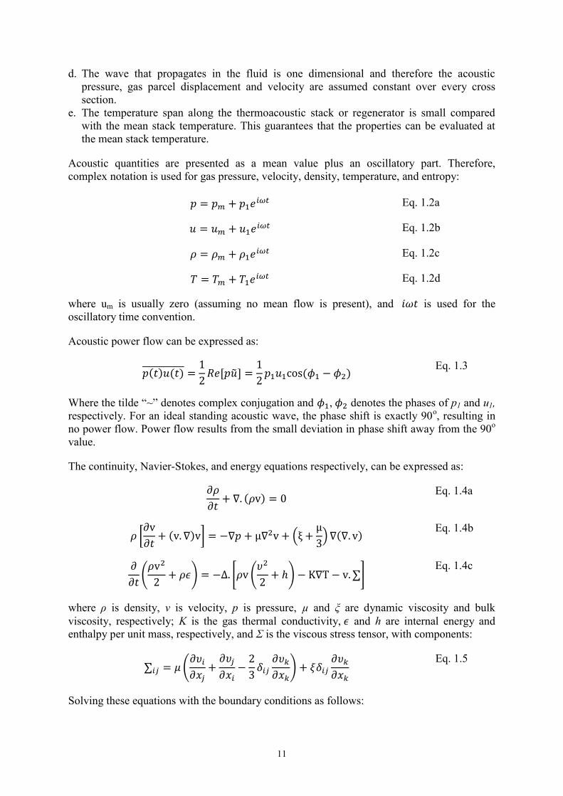
Figure 2.4: Normalized length of the engine stack (Lsn) versus (a) normalized acoustic power
produced (b) normalized thermal efficiency of engine stack, at different normalized stack center
positions (xcn) at normalized temperature difference= 0.7. 23
Figure 2.5: Measurements of the fundamental pressure and the streaming time averaged pressure in
a 70 Hz standing wave by Smith and Swift. 24
Figure 2.6: Effect of inserts on the first harmonic normalized amplitude vs the square of the
normalized fundamental amplitude. 25
Figure 3.1: A schematic drawing of the engine and measurement instrumentation 27
Figure 3.2: The apparatus of the engine in the lab showing the resonator and the measurement
instrumentation. 28
Figure 3.3: Cell geometry of rectangular stack cross section. 29
Figure 3.4: The finned tube heat exchanger inside the resonator developed specially for this study. 31
Figure 3.5: Shapes of inserts used in this experiment 32
Figure 3.6: The power sensor model 8510B-2, and the amplifier model 136 used in pressure signal
detection and processing. 33
Figure 3.7: Oscillations at three different locations visualized simultaneously on the oscilloscope
screen. The figure includes 3 waves obtained from 3 different microphones. 34
Figure 3.8: The pressure amplitude versus time during a full run of the engine including startup,
steady oscillations, and shut-down. 36
Figure 3.9: Thermoacoustic wave in time and frequency domain. 39
Figure 4.1: DELTAEC schematic of the engine. 41
Figure 4.2: (a) Real and imaginary components of dynamic pressure inside the resonator as
predicted by DELTAEC using air at 1 bar and 600-CPSI stack. (b) Real and imaginary components
of volumetric velocity inside the resonator as predicted by DELTAEC using air at 1 bar and 600-
CPSI stack. 42
Figure 4.3: The acoustic and total power flows inside the resonator as predicted by DELTAEC.
Negative values refer to flow in the –x direction. 1:cold duct, 2: cold heat exchanger, 3:stack, 4:hot
heat exchanger, 5:hot duct 43
Figure 4.4: Effect of input heat power on acoustic power output of the engine for air at 1 bar using a 44

IX
600-CPSI stack.
Figure 4.5: Effect of input heat power on the square of the normalized fundamental frequency for air
at 1 bar using a 600-CPSI stack. 44
Figure 4.6: Effect of input heat power on the frequency of the fundamental acoustic wave for air at 1
bar using a 600-CPSI stack. 45
Figure 4.7: The thermal network for the resonator walls, the 600-CPSI stack and the gas filling it.
Rres is the resonator wall thermal resistance, Rstk is the stack walls thermal resistance, and Rgas is
the gas thermal resistance. 46
Figure 4.8: Performance of the thermoacoustic engine using air at 1 bar and a 600-CPSI stack
during a 7200 s run. (a) Temperature of air at the hot and cold sides of the stack and temperature
difference across the stack. (b) Dynamic pressure amplitude of the fundamental wave measured at
14.5 cm from the hot side blind flange during the experiment. 47
Figure 4.9: Dynamic pressure amplitude of the fundamental wave versus the temperature difference
across the stack during a full run of 7200 seconds. The engine uses air at 1 bar and a 600-CPSI stack.
Dynamic pressure is measured at 14.5 cm from the hot side blind flange. 48
Figure 4.10a: Full cycles of engine operating for different times of 300,500, 1700 seconds, showing
transient path of temperature and dynamic pressure amplitude, and the hysteresis loop of dynamic
pressure amplitude with temperature difference. 49
Figure 4.10b: Full cycles of engine operating for different times of 3000 seconds, and 7200 seconds,
showing transient path of temperature and dynamic pressure amplitude, and the hysteresis loop of
dynamic pressure amplitude with temperature difference. 50
Figure 4.11: Full cycle of the engine operating for 3000 s starting from hot condition (upper row)
and cold conditions (lower row) showing transient path of temperature and dynamic pressure
amplitude, and the hysteresis loop of dynamic pressure amplitude with temperature difference. 51
Figure 4.12: Full cycles of engine operating for different gas mixtures of air and Helium, showing
transient path of temperature and dynamic pressure amplitude, and the hysteresis loop of dynamic
pressure amplitude with temperature difference. Red and blue dashed lines are hot and cold
temperatures, while green continuous line is the temperature difference. 52
Figure 4.13: Full cycles of engine operating for different gas mixtures of air and Helium, showing
transient path of temperature and dynamic pressure amplitude, and the hysteresis loop of dynamic
pressure amplitude with temperature difference. Red and blue dashed lines are hot and cold
temperatures, while green continuous line is the temperature difference. 54
Figure 4.14: AC-coupled pressure waves in the time domain at different temperature differences
across the stack at three different axial locations along the resonator 55
Figure 4.15: AC-coupled pressure waves in the time domain at different temperature differences
across the stack at three different axial locations along the resonator 56
Figure 4.16: Density, speed of sound, Prandtl number and thermal conductivity for air/helium gas
mixtures 58
Figure 4.17: Engine output acoustic power flow at three different gas compositions. a. normalized
power and input heat. b. absolute power and input heat. 59
Figure 4.18: Pressure ratio at different gas compositions and different pore sizes. a. 600-CPSI, b.
400-CPSI and c. 200-CPSI measured at 14.5 cm from hot-duct flange. 61
Figure 4.19: Normalized first harmonic amplitude versus normalized squared fundamental
amplitude at different gas compositions and different pore sizes. a. 600-CPSI, b. 400-CPSI and c.
200-CPSI 62
Figure 4.20: The linear behavior normalized first harmonic amplitude versus normalized squared
fundamental amplitude at different gas compositions and different pore sizes. 63
Figure 4.21: Temperature difference between the two sides of the stack versus the heat input for
different gas compositions and different pore sizes. a. 600-CPSI, b. 400-CPSI and c. 200-CPSI
compared to DELTAEC calculations for 100% air. 64

X
Figure 4.22: power carried by the fundamental wave and the first harmonic for the 400-CPSI stack
operated with air as working fluid. Power measured using 2 microphones at 14.5cm and 59.5 cm
from the hot-side blind flange. 65
Figure 4.23: Power and frequency for multiple inserts with various shapes and positions. Solid
columns are measurements, hollow columns are DELTAEC calculations. 66
Figure 4.24: Fundamental amplitude, and normalized ratio (Pm.P1/P02) for multiple inserts with
various shapes and positions. Solid columns are measurements, hollow columns are DELTAEC
calculations. 67
Figure 4.25: Power output and thermal to acoustic efficiency versus heat input to the system with no
insert in the resonator. 68
Figure 4.26: Power output and thermal to acoustic efficiency versus heat input to the system with
50C3 is placed in the resonator 60 cm away from the hot-side flange. 68
Figure 4.27: Effect of normalized position of insert on selected parameters with 400cpsi stack. a)
Output power b) Fundamental pressure amplitude at 14.5 cm from hot-side blind flange c)
Frequency d) First harmonic amplitude along the resonator with and without the insert. Position is
the distance from hot-side flange. 70

XI
List of Tables
Table 3.1: Resonator and stack dimensions 30
Table 4.1: Thermal resistance components in a 600-CPSI stack 46
Table 4.2: The average hydraulic radius to thermal penetration depth ratio for
experiments in figure 5.3. The values are all calculated at mean temperature of
400oC. 60
Table A : Thermal properties of air-He mixtures used in experiments 77

XII
Abstract
Thermoacoustic engine is one of the emerging technologies in the field of energy conversion.
Thermoacoustic engines convert thermal energy, possibly at relatively low temperatures to
mechanical energy in the form of acoustic oscillations of high amplitudes that can drive a
thermoacoustic refrigerator or can be converted to electrical energy using a linear alternator.
In this work, a prototype of a thermoacoustic engine was built, operated and tested.
Sustainable operation of the engine is possible due to the relatively efficient hot and cold heat
exchangers that were able to sustain the temperature gradient across the stack.
Both the transient and steady-state performance of the thermoacoustic engine are investigated
using variable gas mixtures and using square-cell stacks of variable porosities. The engine
performance is studied during full runs consisting of start-up, steady operation, and shutting-
down. The steady-state engine performance and wave characteristics are investigated at
different heat input values, different gas mixtures, and different stack porosities. Inserts with
different patterns and open areas are used inside the resonator to investigate their effect on
suppressing the high harmonics of the produced acoustic wave. A numerical model of the
current prototype is built using the free simulation software DELTAEC. The model is
validated using the experimental data and is then used to obtain more information about the
engine performance.
Results show that the used gas mixture, the pressure ratio, and the stack cell dimensions
significantly affect the engine power output, the wave dynamic pressure amplitude, and the
harmonic content of the wave. Experimental data agrees with DELTAEC calculations in
trend, but the values of acoustic power and dynamic pressure are significantly lower than the
numerical model calculations. The values of the frequency are within 3% of the measured
values.
The transient analysis shows that the dynamic pressure amplitude of the gas reaches a peak
after onset and then decreases to a steady value during the run. The onset temperature of the
engine is always higher than the temperature at which the system stops producing oscillations
while shut-down. The hysteresis characteristics is significantly affected by the thermal
conductivity of the gas mixture, the stack cell dimensions, the mean temperature at starting,
and the time of the cycle. The heat exchange process at the cold side is enhanced by the
existence of the wave.
In this work, several inserts of different thicknesses, open area, positions, and hole patterns
are inserted into the resonator to suppress the harmonics. All inserts caused lower harmonic
content with respect to the case with no inserts. Inserts of low open area cause the
performance to degrade and produce low acoustic powers. Inserts with higher thickness gave
better performance. Amongst all inserts used, the highest acoustic power is obtained using an
insert with an open area of 50% of the resonator area, a pattern of several distributed holes, a
thickness of 3 cm, and at a position of 0.33 of the fundamental wavelength measured from the
cold-side blind flange.

1
1. Introduction
Thermoacoustics is a promising technology that has a rapidly growing field of applications.
Thermoacoustic engines and refrigerators based on the interactions between temperature,
density and pressure variations on the acoustic longitudinal wave are safe, reliable, durable
and environmentally friendly. These applications have the advantages of using no adverse
chemicals, containing no environmentally unsafe contents, having no or few moving parts.
Thermoacoustic devices can readily be driven using solar energy or waste heat and they can
be controlled using proportional control. They can use heat available at low temperatures
which makes it ideal to regeneration using waste heat from engines, and suitable for solar
energy applications. The components included in thermoacoustic engines are usually very
simple compared to conventional engines. The device can easily be controlled and
maintained.
1.1 Thermoacoustics
Thermoacoustics utilizes the rich interactions between thermodynamics and acoustics. In any
sound wave, there exist coupled pressure, displacement, density, and temperature oscillations.
The pressure oscillations induce temperature oscillations which in turn cause heat transfer to
or from nearby solid surfaces. The combination of these oscillations and the placement of
enough solid walls at the proper position in the acoustic wave, close enough to the heated or
cooled areas in the gas, produce a rich variety of thermoacoustic effects.
Nikolaus Rott (1)
gave a definition of thermoacoustics in his review article as “a subject
dealing generally with effects in acoustics in which heat conduction and entropy variations of
a medium play a role”. Thermoacoustics in modern research has a more specific domain
which includes the energy conversion processes dealing with acoustic and heat energies,
namely thermoacoustic engines and thermoacoustic refrigerators. This type of energy
conversion is a fast developing technology that contributes to the global trend towards the use
of renewable energies.
Thermoacoustic engines are devices that use heat to produce mechanical work in the form of
acoustic pressure oscillations. Thermoacoustic refrigerators and heat pumps are devices that
use acoustic work to transfer heat against a temperature gradient to achieve refrigeration or
heating effect. The two types of devices usually contain the same elements: a thermoacoustic
element (a stack), surrounded by hot and cold heat exchangers. The system is housed inside a
resonator. Acoustic drivers are used in refrigerators and heat pumps to drive the refrigeration
effect, while linear alternators are used in engines to harvest the acoustic energy and convert
it into electricity.
The stack is the element in which the main thermoacoustic phenomena take place to produce
or consume acoustic work under a temperature gradient. The thermoacoustic cycle takes
place in the working fluid near the walls of a solid substrate. The stack is an element with
enough channels parallel to oscillation of the gas. The walls of the channel provide more
contact area between the working fluid and the solid which is vital to achieve the correct
phasing between the gas and the solid surface and to complete the thermoacoustic cycle. The
performance of the thermoacoustic stack depends on its material, length, position in the wave,
the geometry of its pores, and its porosity. The porosity is the ratio between the gas open area
and the stack total area, which depends on the number of pores in the area unit and the wall
and pore thicknesses.

2
The thermoacoustic effect inside the stack takes place mainly in the region that is close to the
solid walls of the stack. The layers of gas too far away from the stack walls experience
adiabatic oscillations in temperature that result in no heat transfer to or from the walls, which
is undesirable. Therefore, an important characteristic for any thermoacoustic element is the
value of the thermal and viscous penetration depths. The thermal penetration depth δk is the
thickness of the layer of the gas where heat can diffuse through during half a cycle of
oscillations. Viscous penetration depth δv is the thickness of the layer where viscosity effect
is effective near the boundaries. The ratio of the thermal to viscous penetration depths is the
square root of the Prandtl number. For pure gases at standard pressure and temperature,
Prandtl number is about 0.7, while for mixtures of gases; lower values of Prandtl can be
obtained.
The oscillations of the gas in a standing-wave thermoacoustic engine take the form of a part
of a longitudinal standing-wave. The mode and the frequency of the wave are controlled by
the boundary conditions of the resonator in which the wave is contained. The resonator is a
path of certain geometry where the gas is allowed to oscillate according to the boundary
conditions that control the pressure and particle velocity of the gas. A resonator with a
perfectly closed end forces the oscillations in the velocity of the gas to be zero (a node in the
wave) at the closed end, whereas a resonator with a perfectly open end forces the oscillations
in the velocity of the gas to be maximum (a velocity antinode) at the open end. The
oscillations in the pressure of the gas in a standing-wave with no energy transfer are different
in phase with the oscillations in velocity with 90o. That means that in a non-dissipating
standing-wave, a node of velocity oscillations occurs in the same position with an antinode of
pressure oscillations and vice versa.
Heat is added and removed from the thermoacoustic engines and refrigerators through heat
exchangers. The heat is added or removed from the oscillating gas around the heat exchanger
to ensure that the thermoacoustic stack is under a temperature gradient that allows the
thermoacoustic effect to take place. In the case of oscillating gas, the particle of the gas will
have a maximum displacement in the direction of the temperature gradient. A heat exchanger
with fins longer than the value of this displacement does not make use of the additional fin
space. This puts limitations on the design of the heat exchangers used in thermoacoustics.
In thermoacoustic refrigerators (TAR), acoustic energy is introduced into the system by
acoustic drivers which are devices that convert electric power to acoustic power using a
magnetically-oscillating electric coil. Improving the electro-acoustic conversion efficiency of
these devices is critical to the improvement of the acoustically-driven thermoacoustic
refrigerators. On the other hand, in thermoacoustic engines (TAE) electric power is produced
from the acoustic wave by the movement of a piston in a linear alternator. Alternating current
is produced by these devices at a frequency equal to the frequency of the oscillations.
In thermoacoustically-driven thermoacoustic-refrigerators (TADTAR), the acoustic power is
introduced in the system through a thermoacoustic engine. This technology leads to the
refrigeration with no moving parts. The moving element in this case is just the gas itself. This
increases the reliability and durability of the device.
The first law conversion efficiency in TAE is defined as the ratio between the acoustic power
produced and the heat input to the engine. The second-law efficiency describes the
reversibility of the engine and is defined as the ratio between the first law efficiency and the
Carnot cycle efficiency operating at the same temperature limits.

3
The performance of TAR is characterized by the coefficient of performance (COP) which is
the ratio between the refrigeration of heat pumping heat and the input work to the system.
The ratio of the COP to COP of a Carnot cycle operating at the same temperature limits is
used as an indication of the reversibility of the TAR.
The process of designing a thermoacoustic device became easier using the design
environment (Design environment for low-amplitude thermoacoustic energy converters,
DELTAEC). This software solves the one-dimensional mono-frequency wave equation to
predict the performance of any configuration of thermoacoustic elements. It is used widely in
the design and performance analysis of thermoacoustic devices. The real and imaginary parts
of the dynamic pressure and the volumetric efficiency are matched between at the start of
every segment with the end of the previous segment so that continuity is conserved.
DELTAEC, however, suffers from many drawbacks. It does not take the turbulent losses into
account. It also doesn’t account for minor losses, harmonic content, or streaming.
1.2 Historical review of thermoacoustics
As sound is one of the five senses of the human, acoustics was a field of observations and
research since the early existence of the man on earth. In the 6th
century BC, the Greek
philosopher Pythagoras investigated the differences between the different music instrument
intervals. Aristotle (384-322 BC) was the first one to mention the relation of sound on
contractions and expansions of the air. Around 20 BC, the Roman architect Vitruvius
discussed the effects of echoes and revibration in his treatise about theatre design. Galileo
Galilei and Marin Mersenne were first to understand most of the basic laws of the sound
independently. Newton derived the equations of the sound wave velocity in solids in his book
“Principia” in 1687.
Thermoacoustic-induced oscillations have been observed for centuries. Glass blowers
produced heat generated sound when blowing a hot bulb at the end of a cold narrow tube.
This phenomenon also has been observed in cryogenic storage vessels, where oscillations are
induced by the insertion of a hollow tube open at the bottom end in liquid helium, called
Taconis oscillations, but the lack of heat removal system causes the temperature gradient to
diminish and acoustic wave to weaken and then to stop completely.
Byron Higgins made the first scientific observation of heat energy conversion into acoustical
oscillations. He investigated the “singing flame” phenomena in a portion of a hydrogen flame
in a tube with both ends open. Putnam and Dennis gave a survey of the related phenomena.
Rijke introduced this phenomenon into a greater scale by using a heated wire screen to induce
strong oscillations in a tube. Feldman mentioned in his related review that a convective air
current through the pipe is the main inducer of this phenomenon(2)
. The oscillations are
strongest when the screen is at one fourth of the tube length.
Research performed by Sondhauss in 1850 is known to be the first to approximate the
modern concept of thermoacoustic oscillation. Sondhauss experimentally investigated the
oscillations related to glass blowers. Sondhauss observed that sound frequency and intensity
depends on the length and volume of the bulb.
Lord Rayleigh gave a qualitative explanation of the Sondhauss thermoacoustic oscillations
phenomena, where he stated that producing any type of thermoacoustic oscillations needs to
meet a criteria: “If heat be given to the air at the moment of greatest condensation or taken

4
from it at the moment of greatest rarefaction, the vibration is encouraged”. This shows that he
related thermoacoustics to the interplay of density variations and heat injection.
The formal theoretical study of thermoacoustics started by Kramers in 1949 when he
generalized the Kirchhoff theory of the attenuation of sound waves at constant temperature to
the case of attenuation in the presence of a temperature gradient.
Rott made a breakthrough in the study and modeling of thermodynamic phenomena by
developing a successful linear theory(3)
. After that, the acoustical part of thermoacoustics was
linked in a broad thermodynamic framework by Swift(4)
.
1.3 Linear theory of thermoacoustics
The formulation of the governing equations of thermoacoustics in a general linear theory was
not developed until the 1970s, when Rott was able to present a unifying linear perspective
that can easily be applicable to the thermoacoustic devices(1,3,5-7)
. In this chapter, the linear
theory of thermoacoustics is briefly presented. The linear theory of thermoacoustics makes
use of several assumptions to simplify its formulations. It should be noted that operation of a
thermoacoustic engine at high values of dynamics pressure amplitudes increases the actual
performance deviation away from the predicted performance and introduces many losses that
are not linearly accounted for, thus causing the engine performance to degrade. Nevertheless,
the linear theory provides an important tool to simulate, design, and compare the performance
of the thermoacoustic engines at low amplitudes.
1.3.1 Thermoacoustic phenomena
Acoustic oscillations in a media are a set of time depending properties, which may transfer
energy along its path. Along the path of an acoustic wave, pressure and density are not the
only time dependent property, but also entropy and temperature. Temperature changes along
the wave can be invested to play the intended role in the thermoacoustic effect. The interplay
of heat and sound is applicable in both conversion ways. The effect can be used to produce
acoustic oscillations by supplying heat to the hot side of a stack, and sound oscillations can
be used to induce a refrigeration effect by supplying a pressure wave inside a resonator where
a stack is located.
In a thermoacoustic prime mover, a high temperature gradient along a tube where a gas media
is contained induces density variations. Such variations in a constant volume of matter force
changes in pressure. The cycle of thermoacoustic oscillation is a combination of heat transfer
and pressure changes in a sinusoidal pattern. Self-induced oscillations can be encouraged,
according to Lord Raleigh, by the appropriate phasing of heat transfer and pressure changes.
1.3.2 Thermodynamic cycle
The thermoacoustic cycle can be analyzed by focusing attention on what happens at a given
parcel of a fluid while it oscillates in a resonator where a temperature gradient exists on the
walls. Figure 1.1 shows the cycle of thermoacoustics in a device serving as (a) heat
pump/refrigerator and a device serving as (b) prime mover. For simplicity, the parallel heat
transfer process and compression or rarefaction are separated into different steps to give a
clearer visualization of the cycle. The cycle is therefore found to be identical to the Brayton
cycle.

5
Figure 1.1: Typical cycle of (a) thermoacoustic heat pump and (b) thermoacoustic
prime mover(4)
.
It is important to note that phasing in a traditional heat engine is critical. Pistons or valves
have to move with correct relative motion for the working medium to be transported through
the desired thermoacoustic cycle. Thermoacoustic devices do not contain moving parts to
perform this function, yet the acoustic simulation of heat flux and generation (or absorption)
of acoustic work point to some type of timed phasing of thermodynamic processes achieved

6
in a simple way. Phasing in acoustic devices depends on the presence of two thermodynamic
media: fluid and solid walls.
The dynamic changes of the temperature in the fluid oscillating at the acoustic frequency
come from two superimposed sources: the adiabatic compression and expansion of the fluid
by the acoustic pressure, and the local temperature of the solid walls near the fluid. The heat
flow between the solid walls and the fluid creates a time delay in temperature between
temperature and pressure, which creates the necessary phase shift that drives the
thermoacoustic cycle. Therefore, a rather poor thermal contact between the solid walls and
the fluid parcel is intentionally required to achieve the correct phasing of the temperature
oscillations of the working fluid and solid stack surface. For sinusoidal motion, parcels at a
thermal penetration depth away from the solid walls have the critical phasing needed for the
thermoacoustic effect. Parcels further away have no thermal contact with the walls and are
simply compressed and expanded adiabatically by the wave, while parcels at a thermal
penetration depth from the walls have good enough thermal contact with the walls to
exchange heat with the solid walls but, at the same time, are in poor enough contact to
produce the correct phasing for the cycle. Therefore, the gas at about δk away from the walls
is the main contributor to the thermoacoustic effect as shown in figure 1.2. The thermal
penetration depth is the distance through which the heat can diffuse through the gas in half a
cycle. The thermal penetration depth is a parameter of the thermoacoustic effect, affected by
the properties of gas and the frequency of oscillations. A gas with a high thermal
conductivity, or a cycle with a lower frequency, allows a thicker layer of gas to be effective
for the process.
Figure 1.2: P-V diagrams for the thermodynamic processes of the gas parcels as the
distance from the wall, d, increases.
The cycle needed for the heat pumping effect is illustrated in figure 1.1a. The heat pumping
process is characterized by a low temperature gradient on the walls in contact with the gas
parcel. It can be simplified into the following four processes: [1] Initially, the relatively cold
gas parcel is compressed by the acoustic wave while moving. This reversible process causes
the gas to warm up to the highest cycle temperature and move inwards to become in contact
with the high temperature side of the wall. [2] Due to the low temperature gradient, the gas is
warmer than the hottest portion of the wall. Heat flow irreversibly from the parcel to the wall.
This heat rejection process is accompanied with further contraction that consumes more
work. [3] The cycle continues as the parcel is displaced outwards reversibly to its initial
location, causing the parcel to reach the lowest cycle temperature. The cold parcel is now in
contact with the cold side of the stack wall. [4] However, the temperature of the gas is lower
than that of the wall, thus heat flows irreversibly to the parcel.

7
In a thermoacoustic prime mover, [1] a reversible process of isentropic compression is done
by the wave, consuming input work to the system, and causing the gas parcel to contract and
warm up to a higher temperature. The movement of the parcel while contracting shall put it in
contact with the high temperature wall section. [2] Heat flows from the wall to the parcel in
an irreversible constant pressure process causing the parcel to reach the maximum cycle
temperature. This causes the parcel to rarefy. [3] Consequently, the parcel moves outwards
and work is obtained from the system. Now the parcel cyclic movement is going to make a
reversible expansion process. Output work of this process is equal to the input work of the
compression process, equalizing their share in net work. The parcel has now moved to be in
contact with the coldest portion of the wall. [4] Heat irreversibly flows from the parcel to the
solid walls and the parcel cools down and contracts to its initial condition. This attracts the
parcel inwards again. However, needed work is less than produced work in the second
process, producing net work. As a result, a standing wave is sustained due to the presence of
a temperature gradient. The process follows the criteria of Lord Rayleigh as the addition of
heat occurs when the pressure is high, and the heat is rejected when the pressure is low, thus
encouraging the oscillations.
The main parameter that determines the type of the device (prime mover or refrigerator/heat
pump) is the value of the temperature gradient. A critical temperature gradient is needed to
induce the cycle in the direction of producing net work. This can be explained by considering
processes [1] and [3] in the engine cycle (figure 1.1). The two adiabatic processes are needed
to complete the cycle but result in no net work. The compression and expansion result in a
certain temperature difference for the gas parcel in the two positions it reaches while
expanding and contracting. For the whole media, this results in the need of a certain
temperature gradient for these two processes to occur. The increase in the temperature
gradient over its critical limit provides the necessary values for the two other isobaric
processes to occur, producing the net work of the cycle.
The refrigerator cycle that uses acoustic work to produce adverse heat flow, results in a
temperature gradient lower than the critical temperature gradient needed by the engine. The
ratio of the temperature gradient to this critical temperature gradient is a very important
parameter in the performance of thermoacoustic devices. Pressure oscillations are encouraged
in the gas if a temperature gradient larger than this critical limit is imposed on the plate axial
direction:
Eq. 1.1
where Tm is the mean gas temperature, β is the thermal expansion coefficient, p1, ρ1 and u1
are dynamic pressure, density, and volumetric velocity of the gas respectively and ω is the
angular frequency of oscillations. The ratio between the temperature gradient and the critical
limit is less than one in the refrigerators and higher than one in prime movers. The
thermoacoustic processes depend mainly on the interactions between the oscillating gas and
the fixed, nearly isothermal solid surface. That suggests that the effective gas layer is the
layer that can transfer heat to and from the wall. Gas oscillating far away from the wall
undergoes an adiabatic process, gaining or losing no heat and making no contribution to the
thermoacoustic effect. Gas in perfect contact with the solid surface can be assumed to follow
the temperature of the walls and can be assumed to compress and expand isothermally,
gaining and losing heat to the walls.

8
1.3.3 Acoustic Background
Acoustics is the branch of physics concerned with the mechanical pressure waves we call
“sound”. Acousticians study any mechanical wave that can be transmitted in any medium in
any range of frequency, not only the audible range. Acoustic wave is a form of energy
transfer: It carries energy from a location to another.
Acoustic wave is a type of harmonic oscillations. Harmonic oscillations are repeated
movements where a particle moves around a position of equilibrium. The particle in acoustic
waves is the matter particle and the energy is associated with its movement. The particle
moves back and forth around a stationary position in the same direction of the wave
movement, while the energy of the wave moves across the space.
The following paragraph discusses some of the main parameters that are used to define and
acquire reasonable knowledge of the nature of an acoustic wave.
i. Full Cycle
A particle goes one full acoustic cycle when it reaches a certain position in its oscillatory
movement twice, one moving forth and one moving back as shown in figure 1.3. After one
cycle, the particle reaches its original position at the beginning of the cycle. A standard
position agreed upon to be the typical start of a wave is the equilibrium position, where the
movement around it in both directions are similar.
Figure 1.3: Wave characteristics for a typical sinusoidal wave
ii. Wavelength, frequency, time period, and wave number
Wavelength, λ, is the distance between the consecutive locations along the wave propagation
direction, where the values of the pressure are the same. The frequency, f, of a wave is the
number of cycles that pass through a fixed point in one second. Its unit (Hz) is named after
Hertz and is equal to one cycle per second. The higher frequency is related to higher rate of
energy transfer. For a fixed propagation speed: the higher the frequency, the shorter the
wavelength. Time period, T, of a wave is the time taken by the gas particle to complete a full

9
cycle. It is the inverse of the frequency. The wave number is the number of wavelengths per
2π units of distance. It is sometimes termed the angular or circular wavenumber, but more
often simply as wave number.
iii. Resonance
Resonance is the tendency of the system to produce higher amplitude oscillations at certain
frequencies. These frequencies are known as the system resonance frequencies, or
fundamental frequencies. The same driving force can produce higher pressure amplitudes at
resonance frequencies than when operated at other frequencies.
In a mechanical system comprising an oscillating mass attached to a spring with certain
stiffness, the system tends to oscillate with higher amplitudes at the resonance frequency that
depends on the value of the mass and the stiffness of the spring. If the system is free to
oscillate without external forces, it oscillates at the resonance frequency.
In an acoustic system, the geometry of the resonator in which the wave is contained will
specify the values of the resonance frequencies. The system boundary conditions will specify
a set of wave lengths, and frequencies, at which the particle will oscillate in a way that
satisfies the boundary conditions. The frequencies of resonance of an iso-diameter resonator
are multiples of the fundamental frequency, which is the lowest frequency of oscillations that
satisfies the boundary conditions.
iv. Dynamic pressure amplitude
The amplitude of the wave is the difference between the maximum pressure and the
equilibrium pressure. Although the amplitude of the wave depends mainly on the driving
force which is not dependent on the factors mentioned above, the frequency and energy
transfer are greatly associated with the amplitude. At low dynamic pressure amplitudes, the
linear theory is valid. As the dynamic pressure amplitude increases, non-linear deviations
become dominant.
v. Intensity
Intensity is the rate at which the energy is transferred along the wave path per unit area. It is
mathematically dependent on the driving force along with the parameters of the wave and the
fluid in which the wave moves.
vi. Standing waves
Standing (stationary) wave is a type of wave that remains fixed in space. The amplitude of
oscillation of the particles of the wave for every position does not change with time. The
dynamic pressure at the particles is noticed to have different values in time, but its maximum
(i.e. amplitude) at every point is constant. This occurs as a result of the interference of two
identical waves moving in opposite directions.
The properties of a standing acoustic wave in an air column are illustrated in figure 1.4.
Standing wave contains an amount of energy that is fixed at the location of the wave.
Standing wave needs energy to generate the pressure oscillations, but does not need further
energy to sustain itself in a certain position, except to compensate for viscous losses. In
contrast, traveling waves are not confined to a given space in the medium.

10
Figure 1.4: A standing wave in a column full of air.
1.3.4 General Thermoacoustic theory
Starting with Navier-Stokes and continuity equations, Rott developed a formula to describe
the thermoacoustic oscillations that occur as a result of interactions of heat, viscosity, and
thermal effects in fluids (1,3,5-7)
.
Figure 1.5: Geometry of the simplified parallel plate stacks.
Consider a stack of parallel plate placed in a gas-filled resonator as in figure 1.5. The plates
are of thickness 2l and the spacing between every 2 layers of plates is 2y0. The x axis extends
along the stack parallel to the wave propagation direction. The y axis is perpendicular to the
layers of the stacks. The Rott wave equation is derived considering the following
assumptions:
a. The theory only takes into consideration the linear effects. Any higher order effects, other
than energy transport, which is a second order effect, are neglected. It is worth noting that
second order effects, such as acoustic streaming and turbulence, can have high effects on
performance and are not included in the linear assumption.
b. Oscillating phenomena oscillates harmonically at a single angular frequency ( ). This
means that higher order harmonics of the wave is neglected.
c. The resonator walls and the plates of the stack or regenerator are assumed to be perfectly
rigid.
11
d. The wave that propagates in the fluid is one dimensional and therefore the acoustic
pressure, gas parcel displacement and velocity are assumed constant over every cross
section.
e. The temperature span along the thermoacoustic stack or regenerator is small compared
with the mean stack temperature. This guarantees that the properties can be evaluated at
the mean stack temperature.
Acoustic quantities are presented as a mean value plus an oscillatory part. Therefore,
complex notation is used for gas pressure, velocity, density, temperature, and entropy:
Eq. 1.2a
Eq. 1.2b
Eq. 1.2c
Eq. 1.2d
where um is usually zero (assuming no mean flow is present), and is used for the
oscillatory time convention.
Acoustic power flow can be expressed as:
( ) ( )
( )
Eq. 1.3
Where the tilde “~” denotes complex conjugation and , denotes the phases of p1 and u1,
respectively. For an ideal standing acoustic wave, the phase shift is exactly 90o, resulting in
no power flow. Power flow results from the small deviation in phase shift away from the 90o
value.
The continuity, Navier-Stokes, and energy equations respectively, can be expressed as:
( )
Eq. 1.4a
[
( ) ] (
) ( )
Eq. 1.4b
(
) [ (
) ]
Eq. 1.4c
where ρ is density, v is velocity, p is pressure, µ and ξ are dynamic viscosity and bulk
viscosity, respectively; K is the gas thermal conductivity, and h are internal energy and
enthalpy per unit mass, respectively, and Σ is the viscous stress tensor, with components:
(
)
Eq. 1.5
Solving these equations with the boundary conditions as follows:

12
i) The temperatures in the plates and in the gas are coupled at the solid-gas interface where
continuity of temperature and heat fluxes is imposed. These conditions are respectively
expressed as:
( ) ( ), or (
)
(
) Eq. 1.6
ii) No slip condition: ( ) .
Solving the energy equation, the solid temperature can be expressed as:
( )
[
(
) (
)
] (α
)
(α )
Eq. 1.7
, where
( )
Eq. 1.7b
( )
Eq. 1.7c
√
√
( )
( )
Eq. 1.7d
√
√
(
)
Eq. 1.7e
where δk is the thermal penetration depth of the gas, δs is the solid thermal penetration depth,
and σ is the gas Prandtl number. The function f is called the Rott’s function and it is geometry
dependent. The time averaged can be derived as(8)
:
⟨
⟩ ( (
)
( )( )( ))
|⟨ ⟩|
( )| |
[
(
) (
)
( )( )]
[ ]
Eq. 1.8
where As is the cross-sectional area of the stack material. This important result represents the
energy flux along x direction (wave direction) in terms of Tm(x), p1(x), material properties and
geometry. For an ideal gas and ideal stack εs = 0, this result was observed obtained by Rott.
As can be seen from the energy flux equation, the energy flux consists of three terms: the first
term in p1u1 is the acoustic power, the second term in s1u1 is the hydrodynamic entropy flow,
and the final term is simply the conduction of heat through gas and stack material in the stack
region. The acoustic power absorbed in the stack is(8)
:

13
[ ( )
| | |⟨ ⟩|
( ) ( )
( )| |
( )( )
(
)
( ) ⟨
⟩]
Eq. 1.9
This is the acoustic power absorbed (or produced) in the stack per unit length. The subscript 2
is used to indicate that the acoustic power is a second-order quantity, i.e., the product of two
first-order quantities, p1 and u1.
The first two terms in work equation are the viscous and thermal relaxation dissipation terms,
respectively. These two terms are always present whenever a wave interacts with a solid
surface, and they have a dissipative effect in thermoacoustics. The third term in the equation
contains the temperature gradient dTm/dx. This term can either absorb (refrigerator) or
produce acoustic power (prime mover) depending on the magnitude of the temperature
gradient along the stack. This term is the unique contribution to thermoacoustics.
i. Rott’s function
The properties of the temperature and velocity fields of an oscillatory fluid inside a porous
material are completely built in the thermoacoustic functions, fk and fv. Depending on surface
geometry, the equations that yield these functions take different forms and some of the
specific cases are discussed here. The function fv includes the averaged influence of the
viscous forces on the oscillating gas, in the presence of the walls. This expression is geometry
dependent as shown in figure 1.7.
ii. Boundary layer and short-stack approximations
The thermoacoustic expressions presented in the previous section are complicated to use.
Common theoretical assumptions are used to simplify these expressions(8)
.
First, in the boundary-layer approximation the stack pores are of a width y0 >> , so that
the hyperbolic tangents in equation 1.6 can be set equal to unity.
Second, In the short-stack approximation, the stack is considered to be short enough
that the pressure and velocity in the stack do not vary appreciably.
In the standing-wave thermoacoustic engines, the correct phasing between the temperature of
the walls and the gas needs that the absolute value of the imaginary part of fk is high. As
shown in figure 1.6, the optimum point occurs at the point where rh/k is about unity. The
absolute value of the imaginary part is highest and occurs at rh/k of about 2 for the case of
pin arrays which has the highest contact area with the gas.

14
Figure 1.6: Imaginary and real parts of the Rott function fk as function of the ratio of
the hydraulic radius and the thermal penetration depth. Three geometries are
considered. For pin arrays, an internal radius ri = 3δk is used in the calculations(14)
.
The standing-wave acoustic pressure in the stack, , is an appropriate reference for
calculations, and thus, can be taken as real and is given by
( ) Eq. 1.10a
and the mean gas velocity in the stack in x direction is:
(
)
( )
Eq. 1.10b
where p0 is the pressure amplitude at the pressure antinodes of the standing wave and k is the
wave number. The factor (1+l/y0) accounts for the different gas cross sectional areas between
the stack and the resonator, which requires that the velocity inside the stack must be higher
than that outside by the cross-sectional area ratio (1 + l/y0). The Rott’s function f in the
boundary layer-approximation is given by(8)
:
( )
Eq. 1.11a
( )
Eq. 1.11b

15
Equations 1.7 and 1.8 are converted into
( )
( ) (
( )
( )
√
√
( √ √ ))
Eq. 1.12
and
( ) ( ) (
( )
( )( √ ) )
√ ( )
Eq. 1.13
where √
Eq. 1.13b
Boundary and short stack approximations are used to simplify the calculations required to
describe the performance of the gas layers during the oscillations. While the initial forms are
complicated and contain Bessel functions, using the short-stack and the boundary-layer
approximations causes calculations of thermal and acoustic powers to be easier and require
less effort. These approximations are valid in most practical cases.
1.4 Standing-wave Thermoacoustic Engine
The thermoacoustic engine (TAE) is a device that converts heat energy into work in the form
of acoustic energy. A thermoacoustic engine is operating using the effects that arise from the
resonance of a standing-wave in a gas. A standing-wave thermoacoustic engine typically has
a thermoacoustic element called the “stack”. A stack is a solid component with pores that
allow the operating gas fluid to oscillate while in contact with the solid walls. The oscillation
of the gas is accompanied with the change of its temperature. Due to the introduction of solid
walls into the oscillating gas, the plate modifies the original, unperturbed temperature
oscillations in both magnitude and phase for the gas about a thermal penetration depth
√ away from the plate(4)
, where k is the thermal diffusivity of the gas and ω=2πf is
the angular frequency of the wave. Thermal penetration depth is defined as the distance that
heat can diffuse though the gas during a time 1/ω. In air oscillating at 1000 Hz, the thermal
penetration depth is about 0.1 mm. Standing-wave TAE must be supplied with the necessary
heat to maintain the temperature gradient on the stack. This is done by two heat exchangers
on both sides of the stack.
Thermoacoustic engines still suffer from some limitations, including that:
The device usually has low power to volume ratio. Very high densities of operating fluids
are required to obtain high power densities,
The commercially-available linear alternators used to convert acoustic energy into
electricity currently have low efficiencies compared to rotary electric generators, and only
expensive specially-made alternators can give satisfactory performance.
TAE uses gases at high pressures to provide reasonable power densities. This imposes
sealing challenges particularly if the mixture has light gases like helium.
The heat exchanging process in TAE is critical to maintain the power conversion process.
The hot heat exchanger has to transfer heat to the stack and the cold heat exchanger has to

16
sustain the temperature gradient across the stack. Yet, the available space for it is
constrained with the small size and the blockage it adds to the path of the wave. The heat
exchange process in oscillating media is still under extensive research.
The acoustic waves inside a thermoacoustic engines operated at large pressure ratios suffer
many kinds of non-linearities such as turbulence which dissipates energy due to viscous
effects, harmonic generation of different frequencies that carries acoustic power in
frequencies other than the fundamental frequency.
The performance of thermoacoustic engines usually is characterized through several
indicators as follows:
The first and second law efficiencies, defined in section 3.4.3
The onset temperature difference, defined as the minimum temperature difference across
the sides of the stack at which the dynamic pressure is generated,
The frequency of the resultant pressure wave, since this frequency should match the
resonance frequency required by the load device, either a thermoacoustic refrigerator/heat
pump or a linear alternator,
The degree of harmonic distortion, indicating the ratio of higher harmonics to the
fundamental mode in the resulting dynamic pressure wave, and
The variation of the resultant wave frequency with the TAE operating temperature
1.5 Applications
Although the field of thermoacoustics is still in the technical development stage, some
effective devices were built investing the thermoacoustic effect in applications involving
refrigeration or power generation.
In 2007, Babaei and Seddikui(9)
presented a thermoacoustic air refrigeration system designed
for automotive applications, working with helium and investing the engine waste heat with an
overall efficiency of 18.8%.
In 2004, Symko et al.(10)
proposed a small, high-frequency thermoacoustic refrigerator that is
driven by a thermoacoustic engine that uses the waste heat of microelectronic components to
pump heat or produce spot cooling. They proposed using the waste heat from a
microelectronic processor to drive a small scale thermoacoustically-driven thermoacoustic
refrigerator to produce spot cooling for the surface of the processor. Cooling power densities
of 0.1 to 0.6 Watts for every cm2 of resonator cross sectional area were achieved.
In 2004, Hatazawa et al.(11)
designed a thermoacoustically-driven thermoacoustic refrigerator
that uses waste heat from a gasoline engine. In 2007, Babaei et al.(12)
proposed a similar
system to use in a gas turbine trigeneration system, operating with the gas turbine waste heat.
In 2005, Zoontjens et al.(13)
investigated the feasibility of using the automotive motor waste
heat to power a thermoacoustic air conditioner to replace the fuel consuming conventional
system.
In 1998, the first solar-energy powered standing wave thermoacoustic engine was built by
Chen and Garrett(14)
. Adeff and Hofler(15)
built and tested a prototype thermoacoustic system
that operates on the solar energy. Chen(16)
constructed the first solar powered thermoacoustic
cooler which was heated by a parabolic dish collector. Shen et al.(17)
investigated the
performance of a solar-powered thermoacoustic engine working with different gases under
different solar tilt angles.

17
1.6 Thesis Scope
The present study aims to:
[1] build, operate and test a standing-wave engine prototype,
[2] simulate the performance of the built prototype using DELTAEC,
[3] operate the prototype with different gases and gas mixtures, and record the relevant
parameters in transient and steady-state phases,
[4] analyze the engine performance in time and frequency domain in transient and steady-
state phases,
[5] evaluate the performance of the engine and identify the major power losses,
[5] identify the major losses in the engine and its source, and
[6] develop and test a technique to eliminate or reduce the losses in the engine.
In this work, the major source of losses in the engine was identified as the existence of higher
harmonics in the output acoustic wave. The loss in higher harmonic generation was reduced
using inserts of different shapes, blockage areas and positions along the wave.

18
2. Review of Related Literature
The field of thermoacoustic built up a solid base of available literature in the recent decades.
In this chapter, studies of the standing-wave thermoacoustic engines are presented, describing
the history, experimental performance, and simulation results of thermoacoustic engines.
Several studies discuss the validity of the currently accepted theoretical model, the linear
theory. Some authors discuss the possibility of introducing the non-linear terms in the theory.
In the presented literature, experimental performance of many prototypes is compared with
the numerical simulations of DELTAEC software. Other presented studies describe the losses
related to the generation of higher harmonics. Performance and description of several
prototypes built to make use of solar or waste energy are presented.
2.1 Historical background of thermoacoustic engines
The first description of the acoustic-oscillation production using thermoacoustics is described
by Sondhauss in 1850, who detected sound generation in a duct where sufficiently large axial
temperature gradient is imposed. After Byron Higgins made the first observations and
investigations of organ-pipe type oscillations, known as .singing flames, in 1777, the physics
of thermoacoustic were investigated by Kirchhoff in 1868.
No noticeable further progress was made until the thermoacoustic theory was first developed
by Rott(5-7)
and reviewed later by Swift(4)
. In this series of theoretical studies, Rott managed
to build the thermoacoustic theory that describes the interactions of acoustic waves and
temperature variations and the thermodynamic processes associated with the existence of
waves in a fluid. Several research teams aim to improve the effectiveness of this technology
to provide effective alternatives for conventional power production and conversion
technologies.
From as early as 1962, it was experimentally found by Carter et al. that by properly inserting
a solid substrate in the Sondhauss tube, the oscillations were enhanced. Merkli and
Thomann(18)
found that during a thermoacoustic cycle, heat is transferred along a resonator
from a region near the velocity antinode to a region near the adjacent pressure antinode.
These phenomena were studied by Rott(1,3,5-7)
who extended the qualitative explanation by
Lord Rayleigh by giving a quantitative explanation for the phenomena.
2.2 Performance of standing-wave thermoacoustic engines
Standing-wave thermoacoustic engines have been going under extensive research. Although
there has been much progress in the field of travelling-wave engines that is promising
regarding the higher efficiencies, the standing-wave engines possess a lot of advantages that
makes it still competitive. These advantages include simplicity, ease of design and
manufacture, and higher understanding of the physics. Investigations on the non-linear
performance of standing-wave engines still need more work to clearly understand and
describe losses and deviation from the linear theory.

19
2.2.1 Experimental investigations on thermoacoustic engines
Swift(4)
systematically expanded and summarized the theory of linear thermoacoustics. The
theory supposes that the time dependence of all fluctuating quantities, such as pressure,
velocity, temperature is purely sinusoidal. Swift(19)
introduced viscous resistance, thermal-
relaxation resistance, inertance, compliance and proportionality coefficient of a controlled
source to thermoacoustics, and sound-current analogy was carried out.
Arafa et al.(20)
studied the effect of mean pressure and stack length, position, and porosity, on
the performance of a standing-wave engine working with helium from 1 to 10 bar. They
suggested that the engine should work using an inert gas with high speed of sound and low
Prandtl number; the engine should also be operated at a ratio of pore half width to thermal
penetration depth in the approximate range of 3 - 5 for low onset temperature and high
conversion efficiencies.
The use of a dimensionless framework was carried by Olson and Swift(21)
who used
dimensionless parameters to analyze thermoacoustic devices. Dimensionless numbers are
used to reduce the number of independent parameters in their experiments and for scaling
purposes.
The review by Swift(4)
in 1988 described the theoretical performance of thermoacoustic
engines. Theoretical predictions of the linear theory showed that the efficiency and work flux
decrease when the stack is located closer to the velocity node for the same wave length ratio
due to the higher viscous losses and longitudinal thermal conduction. Swift also noticed that
the maximum relative efficiency and maximum work flux do not coincide, but there is a wide
range of acceptable operating conditions. Measurements confirmed the validity of
calculations. The square of normalized pressure increased linearly with the input power at
low amplitudes. Swift expected that at higher amplitudes the nonlinearities will appear, but
couldn’t operate the engine to prevent catastrophic damage due to oscillation-caused
cavitation.
In their paper that describes a solar–driven standing-wave thermoacoustic engine, Chen and
Garrett(14)
confirmed the linear behavior of the square of pressure versus heat input that is
predicted by the linear theory as shown in figure 2.1. The results also showed that the
temperature difference across the stack is essentially independent of input heater power above
onset.
Jin et al.(22)
investigated the performance of a standing wave engine of low onset temperature.
Results of experiments showed the operating characteristics of their prototype. Results
confirmed that the onset temperature of the present system can be lower than 100 °C. The
structural parameters, including stack position and tube inclination, may also affect the onset
temperature. The lowest value can be observed at a proper stack position in a horizontal
resonant tube. As to operating frequency, the resonant tube length is its crucial factor, while
there is little influence from heat input and stack’s position.

20
Figure 2.1: Square of pressure wave amplitude versus heat input to the standing-wave
engine by Chen and Garrett(14)
.
In a detailed work, Swift(23)
presents measurements and analysis of a 13-cm diameter
standing-wave thermoacoustic engine. The engine uses Helium at 13.8 bar. The engine
delivers up to 630W of acoustic power. Swift’s measurement agreed with the predictions of
linear theory within 4% at low acoustic amplitudes. The measurements of the square of the
amplitude, shown in figure 2.2, differ from the predictions by 20%, twice the uncertainty.
Swift suggests some reasons of this deviation including resonance-enhanced harmonic
content in the acoustic wave, and a first order temperature defect in thermoacoustic heat
exchangers. It was observed that at low pressure amplitudes, steady-state operation of the
engine was not possible, because as the heater heated the hot heat exchanger and nearby
parts, causing the engine to begin oscillation quickly reaching high dynamic pressures, and
then these high-amplitude oscillations quickly cooled the hot-stack side causing the
oscillations to stop.
Ibrahim and Abdel-Rahman(24)
presented experimental data on the issues related to operating
the engine by various heat sources at different temperatures. They demonstrated how the use
of gas mixtures affected the onset temperature, the acoustic power output, the operating
frequency, and the change in operating frequency with temperature.
Belcher et al.(25)
numerically assessed thermoacoustic engines using different gases and
concluded that if all losses outside the stack are negligible (in the heat exchangers and
resonator), the minimum onset temperature would occur for gases having a specific-heat ratio
close to one, which is characteristic of polyatomic gases.
2.2.2 Numerical studies on thermoacoustic engines using DELTAEC
Ward and Swift(26)
developed a program for thermoacoustic computation, i.e. DELTAEC
(Design Environment for Low-amplitude Thermoacoustic Energy Conversion), which can be
used to simulate and design thermoacoustic engines and refrigerators, and is helpful for
practical application of linear thermoacoustics.
Valuable contributions by Swift and Ward(27)
to the simulation of thermoacoustics focused on
the theoretical performance of porous stacks, the influence of turbulent flow on viscous
resistance, local loss caused by the variety of flow area, entrance effect and joining condition.
Pa
2 (
Pa
2)
Qin (W)

21
Their work improved the veracity accuracy of the simulation of thermoacoustic machines
within linear thermoacoustics.
Figure 2.2: Square of end pressure amplitude versus input heat for different Helium mean
pressures. Lines are calculations and points are measurements(23)
.
Gardner and Swift(28)
used DELTAEC to calculate values with which to compare the
measurements in their investigation of a cascade thermoacoustic engine. For one of the data
sets, they compared the calculated results for ‘‘as-built’’ dimensions and ‘‘as-running’’
dimensions, to investigate whether thermal expansion of the hot parts and consequent
compression of the bellows were significant. Differences were only of the order of 0.1% and
0.1°, so they performed all other calculations using as-built dimensions. Figure 2.3 shows that
DELTAEC results were close to the experimental measurements. It is important to note that
swift used the minor losses factor as an adjusting parameter for the DETAEC calculations to
meet the measurements.
Ibrahim et al. used DELTAEC to study the performance of a standing-wave thermoacoustic
engine(29)
. They concluded that mean pressure, stack spacing, stack mid-position and stack
length have a noticeable effect on energy conversion efficiency. By compromising the effects
of these parameters, the first law efficiency of their modeled engine could be increased from
9.6% to 16%.
Arafa et al.(30)
used DELTAEC to investigate the sensitivity of the mean pressure, stack
spacing, stack mid-position and stack length on the engine performance. They indicated the
relative importance of these parameters and their effect on the engine performance.
Babaei and Siddiqui used DELTAEC as verification for a design procedure for
thermoacoustic devices. A good agreement is observed between the developed procedure and
the DELTAEC simulations(31)
. Both Wetzel(32)
and Besnoin(33)
discussed thermoacoustic
device optimization in their works. While Wetzel focused on the optimal performance of a
thermoacoustic refrigerator, Besnoin targeted heat exchangers. In addition to these

22
optimization efforts, Zoontjens et al.(34)
illustrated the optimization of thermoacoustic
devices; they used DELTAEC to vary individual parameters to determine optimal designs.
Ueda(35)
determined the effect of a variation of certain engine parameters on pressure
amplitudes. Another work that made use of DELTAEC is Tijani et al.(36)
, who attempted to
optimize the spacing of the stack.
Figure 2.3: Acoustic power flowing through the resonator in terms of the acoustic
power dissipated in an acoustic load. Symbols are measurements and the solid line is
DELTAEC calculations(28)
.
Babaei and Siddiqui(31)
developed a comprehensive design and optimization algorithm for
designing thermoacoustic devices. The results from the algorithm are in good agreement with
that obtained from the computer code DELTAEC. Figure 2.4 describes the results of model in
the study. It shows that at a given stack position, the acoustic power produced by the engine
decreases with an increase in the stack length, whereas, as a given stack length, the acoustic
power produced by the engine increases as the stack moves away from the pressure antinode.
The results show that at a certain combination of certain stack position and length, the stack
performance is the best. Figure (2.4a) shows that every combination of stack positions and
lengths has a limit on the possible acoustic power.
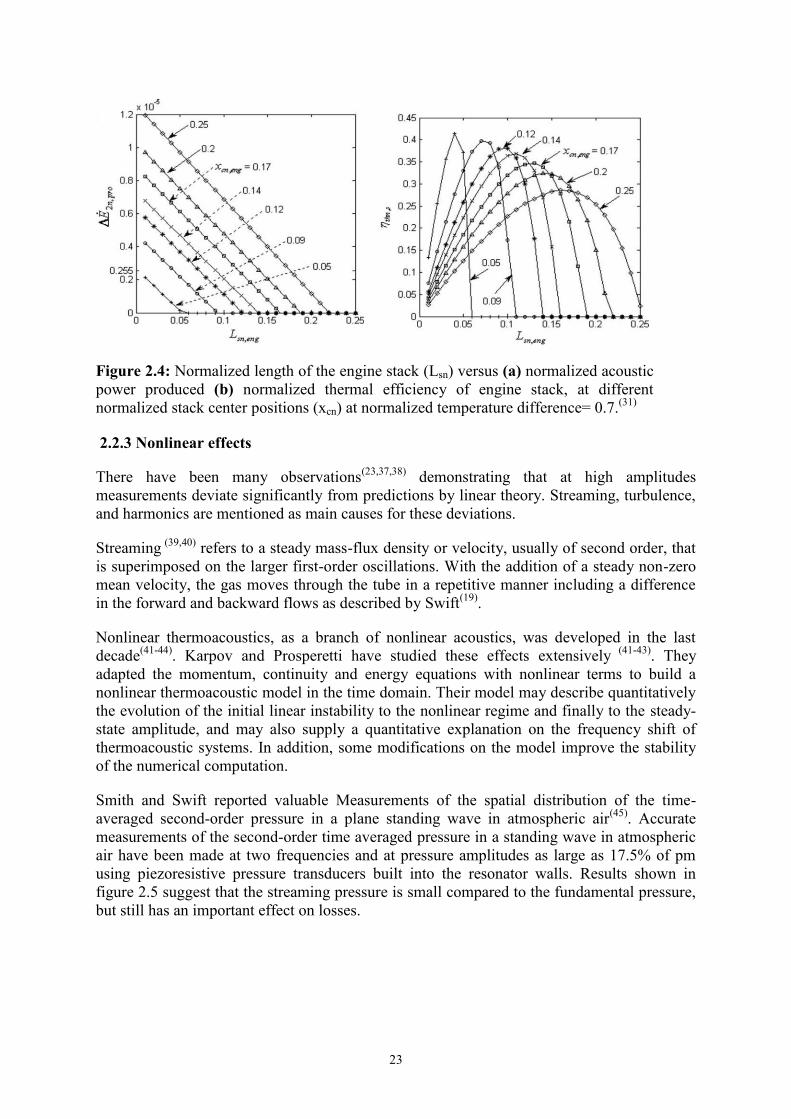
23
Figure 2.4: Normalized length of the engine stack (Lsn) versus (a) normalized acoustic
power produced (b) normalized thermal efficiency of engine stack, at different
normalized stack center positions (xcn) at normalized temperature difference= 0.7.(31)
2.2.3 Nonlinear effects
There have been many observations(23,37,38)
demonstrating that at high amplitudes
measurements deviate significantly from predictions by linear theory. Streaming, turbulence,
and harmonics are mentioned as main causes for these deviations.
Streaming (39,40)
refers to a steady mass-flux density or velocity, usually of second order, that
is superimposed on the larger first-order oscillations. With the addition of a steady non-zero
mean velocity, the gas moves through the tube in a repetitive manner including a difference
in the forward and backward flows as described by Swift(19)
.
Nonlinear thermoacoustics, as a branch of nonlinear acoustics, was developed in the last
decade(41-44)
. Karpov and Prosperetti have studied these effects extensively (41-43)
. They
adapted the momentum, continuity and energy equations with nonlinear terms to build a
nonlinear thermoacoustic model in the time domain. Their model may describe quantitatively
the evolution of the initial linear instability to the nonlinear regime and finally to the steady-
state amplitude, and may also supply a quantitative explanation on the frequency shift of
thermoacoustic systems. In addition, some modifications on the model improve the stability
of the numerical computation.
Smith and Swift reported valuable Measurements of the spatial distribution of the time-
averaged second-order pressure in a plane standing wave in atmospheric air(45)
. Accurate
measurements of the second-order time averaged pressure in a standing wave in atmospheric
air have been made at two frequencies and at pressure amplitudes as large as 17.5% of pm
using piezoresistive pressure transducers built into the resonator walls. Results shown in
figure 2.5 suggest that the streaming pressure is small compared to the fundamental pressure,
but still has an important effect on losses.

24
Figure 2.5: Measurements of the fundamental pressure and the streaming time
averaged pressure in a 70 Hz standing wave by Smith and Swift(45)
.
Higher harmonics oscillate at integer multiples of the fundamental frequency, and can
become quite important at high amplitudes. Atchley et al.(46)
, noticed experimentally that the
generation of higher harmonics can cause highly nonlinear waveforms that degrade the
performance significantly. The impact of the harmonics is greatest when excited near
resonance, but Gaitan and Atchley(47)
suggested that this can be suppressed by careful tuning
of the resonator. A complete numerical extension would require going up to fourth order in
the asymptotic expansion(48)
.
Swift(23)
investigated a way to suppress the losses that dissipate with the harmonics of the
fundamental. He inserted some objects at positions where the amplitude of the first harmonics
is high. The result, plotted in figure 2.6, showed a constant relationship between the first
harmonic amplitude versus the square of the fundamental amplitude, both normalized by the
mean pressure. The constant of the linear relationship decreased when the inserts were used.
Swift(23)
also noticed that inserting blockage in the way of the thermoacoustic wave can affect
its harmonic content. The blockage suppressed the first harmonic when it was put in a point
of the system where the first harmonic has maximum gas-particle velocity. However, Swift
did not discuss the geometry of the insert or its effect on the acoustic-power output of the
system.
Turbulence arises at high Reynolds numbers, where the assumption of laminar flow is no
longer valid. Turbulence may also arise due to abrupt changes in the shape or direction of the
channels, which leads to the shedding of vortices(49,50)
and can cause significant losses.
Gardner et al.(51)
gave some suggestions on how to include turbulence into the modeling, but
they are by no means complete. The available literature suggests therefore that it is still a
challenge to include the effects of turbulence, hysteresis and higher harmonics systematically
into the analysis.
Ibrahim et al.(52)
experimentally investigated the excitation of higher harmonics. They
observed that operating the engine at a temperature just above the onset temperature
generates an acoustic wave at the fundamental mode with no harmonics observed but with
relatively low dynamic pressure amplitude. When they operated the engine at higher

25
temperature differences across the stack, up to 30 % of the generated acoustic power was
contained in the first mode, in their range of operation.
Figure 2.6: Effect of inserts on the first harmonic normalized amplitude vs the square
of the normalized fundamental amplitude(23)
.
2.3 Applications
As a result of more than two decades of attempts, thermoacoustic conversion efficiencies
have been improved to levels that rival what can be obtained from internal combustion
engines(53)
. Some thermoacoustic devices have been successfully applied on space shuttles
and navy warships, but more extensive commercial applications are still restricted by the
power density and actual efficiency (54)
.
In the 1980s, Los Alamos Natioal Laboratory started to develop thermoacoustic devices
including a standing wave thermoacoustic engine build and studied by Swift(23)
. The length
and inner diameter of its resonant tube is 4320 mm and 127 mm, respectively. The system
was charged with gas helium of 13.8 bar. The acoustic power of 630 W was obtained from a
heat input of 7 kW, i.e. its efficiency reached 9%.
Due to the low energy density of thermoacoustic devices, the priority was given to inspecting
their potential to be driven by waste heat or solar energy.
In 1998, the first solar energy powered standing wave thermoacoustic engine (shown in
figure 2.7) was built by Chen and Garrett(14)
. Sunlight was focused, by a 3-feet-diameter lens,
to one end of a ceramic stack, which was located inside resonant tube of 40 cm in length.
This ¼ wavelength resonant can emit sound at 420 Hz, with an intensity of 120 dB at a point

26
1 m distance from the open end of the tube. The onset for the quarter-wavelength mode
occurred at 35 W. This demonstrative prototype proved the feasibility of thermoacoustic
engines driven by solar energy, which is clean and environmentally friendly. The promising
project accords with the global policy of sustainable development and energy saving.
Adeff and Hofler(15)
built and tested a prototype of a thermoacoustically-driven
thermoacoustic refrigerator that operates by solar energy. Chen(16)
constructed a solar
powered thermoacoustic cooler which was heated by a parabolic dish collector. The operating
gas was a mixture of 18% argon and 82% helium at a pressure of six bar absolutes. However,
the cooler just achieved 1.5 oC temperature span due to gas leakage and thermal losses. Shen
et al.(17)
investigated the performance of a solar-powered thermoacoustic engine working with
different gases under different solar tilt angles. Efforts have been made to explore the
possibility of using thermoacoustic engines in waste heat management.
A wide variety of standing-wave engines has been built making use of Rott’s Theory.
Hatazawa et al.(11)
designed a thermoacoustically-driven thermoacoustic heat pump that uses
waste heat from a gasoline engine. The performance of the engine is almost equal to the use
of an electric-heater at a thermal input of 300 W, which corresponds to slightly more than
1% of the heat quantity of exhaust gas provided under typical automobile engine working
conditions. Babaei et al.(12)
proposed a similar system to use in a gas turbine trigeneration
system, operating with the gas turbine waste heat. They proposed system including a
standing-wave engine that drives a standing-wave refrigerator. Preliminary results show that
the thermoacoustic refrigeration system is capable of achieving an overall theoretical
efficiency of 36%. The trigeneration system overall efficiency was enhanced by 5% after the
introduction of the thermoacoustic device. Zoontjens et al.(13)
investigated the feasibility of
using the automotive motor waste heat to power a thermoacoustic air conditioner to replace
the fuel-consuming conventional system. They argue that this proposed system has a strong
potential to replace the conventional automotive air conditioning systems. Symko et al.(10)
proposed a small, high-frequency thermoacoustic refrigerator that is driven by a
thermoacoustic engine that uses the waste heat of microelectronic components to pump heat
or produce spot cooling. They suggest that devices like that can be operated in the range of
ultrasonic frequencies thus working on high power densities.
2.4 scope of the present study
This work aims at developing a thermoacoustic engine, to characterize the engine
performance using different gases and to improve the engine performance by inserting
specially-designed inserts of different blockage area, shapes, thicknesses, and at different
positions inside the resonator. These inserts are designed to suppress the excitation of
harmonics. This is partly a continuation of the work of Swift(23)
in order to study the effect of
these inserts on the harmonic suppression.

27
3. Experimental Setup and Procedure
The experimental setup consists of an iso-diameter resonator filled with a gas mixture. It
contains a thermoacoustic stack and hot and cold heat exchangers. Measurement devices
included pressure, temperature are used and connected to sensors to measure signal
conditions and data acquisition. Data is manipulated and analyzed using codes written using
MATLAB programming language. Detailed description of the apparatus, methods,
measurement procedures, data manipulation and analysis is included in this chapter.
3.1 Standing wave thermoacoustic engine
The used engine is described in figure 3.1. It consists of a resonator with a length of 0.95 m
and a uniform inner diameter of 0.127 m. A stack of length 0.04 m is positions at a center
position of 0.05 m measured from the blind flange. Heat is provided to the system by an
electric heater, connected through a variable resistance, at the stack end closer to the blind
flange. A finned tube heat exchanger is attached to the other side of the stack to absorb the
rejected heat load and to maintain the temperature gradient along the stack. The components
of the apparatus, shown in figure 3.2, and the procedures of measurements and operation are
detailed in the sections of this chapter.
Figure 3.1: A schematic drawing of the engine and measurement instrumentation
3.1.1 Resonator
The resonator is responsible for housing the working gas, the stack, and the hot and cold heat
exchangers. The resonator used is made of a stainless steel tube of 0.950m in length and
0.127m (5 in) in diameter. The resonator shape and dimensions determine the characteristics

28
of the wave. The modes of the wave depend on the boundary conditions at the resonator ends.
For the case of an iso-diameter resonator with blind flanges in both sides, the wave
fundamental mode will be in the form of half a wave length, and its harmonics (n * λ/2,
where n is an integer).
The resonator is filled with the working gas. The low diameter to length ratio (0.13)
guarantees the validity of the one-dimensional assumptions used in DELTAEC.
Figure 3.2: The apparatus of the engine in the lab showing the resonator and the
measurement instrumentation.
3.1.2 Thermoacoustic Stack
The stack which consists of many parallel passes for the air of specially selected dimensions
keeps the operating gas in an effective thermal contact with the walls. The gas carries heat
from adjacent pore walls and transfers it along the stack. Stacks as in figure 3.3 in the used
apparatus have square pores of different sizes detailed in table 3.1.

29
Figure 3.3: Cell geometry of rectangular stack cross section.
The stack is made of celcor. This material shows a high mechanical strength at high operating
temperature, thermal stability and a uniform porosity. This material has a wide range of
applications in many areas such as diesel filter panticulates(55)
. It was supplied by companies
that produce them for this purpose. Celcor has a thermal conductivity k of 2.5 W/K m and its
specific heat cp is 896 J/Kg K(55)
.
The used stacks are cut into pieces of 0.05 m in length and of diameter close to the inner
diameter of the system (0.127 m) using a center lathe and wrapped in a layer of insulating
cloth to decrease the heat transfer between the stack and the conductive resonator body and to
provide good sealing between the stack and the resonator body. Table 3.1 lists the parameters
of resonator and the available stack used throughout the experiments.
3.1.3 Heat exchangers
The heat exchangers are one of the main components of any thermoacoustic device. Energy
input and rejection from the device are vital to keep the temperature gradient along the stack
higher than the critical temperature gradient needed to maintain the thermoacoustic effect. In
a thermoacoustic heat exchanger, thermoacoustic oscillations are the main motion of the gas
that enhances heat transfer(4)
. Swift recommends that the dimension of the heat exchanger
parallel to the wave propagation direction, i.e. its length, should be equal to one peak-to-peak
gas displacement (2 ). Where TD is the gas parcel displacement through half a
cycle, and is the thermal penetration depth(4)
.
In contrast to a steady-flow device, heat transfer cannot be enhanced by lengthening the
traditional heat exchanger passages more than one peak-to-peak gas displacement because
some of the gas in the heat exchanger will never contact the end of the regenerator to deliver
heat where it is required. Instead, the effective way to increase the heat transfer depends on
increasing the number of passages in which the gas flows(57)
. Each passage must be
hermetically sealed from the external fluid passage. The higher the number of passages, the
higher the probability of failure and the cost of fabrication become. In steady-flow devices,
Cel
l
half
th
ick
nes
s
Wall
half
th
ick
nes
s

30
the heat exchangers can be well separated by piping runs, but the small gas displacement also
forces the heat exchangers to be located close together. The compact size and high heat flux
of traditional oscillating-flow heat exchangers often leads to high thermal gradients and high
thermal stresses that promote failure.
Table 3.1: Resonator and stack dimensions
Main Dimensions
Resonator length 92.5 cm Hot duct length 12.5 cm
Resonator diameter 12.7 cm Cold duct length 80 cm
Stack center position 15 cm Stack length 5 cm
Hot heat exchanger
length 1 cm Cold heat exchanger length 1 cm
Dimensions of used stacks
CPSI 200-CPSI 400-CPSI 600-CPSI
Plate spacing (µm) 771 559 481
Plate thickness
(µm) 127 76 38
Porosity 73.7% 77.5% 85.8%
The heat exchanger used in the apparatus is shown in figure 3.4. It consists of 11 parallel
vertical copper tubes of 1 cm diameter. Circular copper rings of 1 mm thickness are attached
around each tube at spacing of 1mm. The heat exchanger width (in direction of resonator
axis) should be selected equal to the particle displacement which is around 2mm in this
case(19)
. However, due to the simple manufacturing techniques used, the width of 1cm is used.
The extra width does not help as heat transfer surface area, but it allows for wider tubes and
minimizes cooling water flow resistance.
3.1.4 Working gas
Working gas is selected upon the working case conditions. For a certain frequency and mean
pressure and temperature, every gas has its thermal and viscous penetration depths. The
selection of stack pore dimension depends on these depths.
The power densities that can be transferred in a gas depend on its density and molecular
weight. This suggests that for a certain level of output power required, a gas of proper density
will be needed. Practical thermoacoustic devices use high pressure gases as mean gas
pressure can alter the density, but it increases the weight, viscosity, and leakage probability of
the gas.

31
Figure 3.4: The finned tube heat exchanger inside the resonator developed specially for this
study.
No certain mixture is known to give the best performance in thermoacoustic devices.
Mixtures of low Prandtl number is suggested to give higher performance, but the best
performance are not necessarily obtained by using the mixture of lowest Prandtl number. The
engine efficiency increase is a consequence of two effects:
i. The Prandtl number decrease.
ii. the output power is proportional to the acoustic velocity u and thus inversely proportional
to the product of the density and velocity of sound ρa (in a standing wave: u ∼ p/ρa).
Lowest Prandtl number usually occurs in mixtures of binary gases. As the gases are not of
the same density, the mixture with the lowest Prandtl number is not the mixture with lowest
possible density, and the best performance is obtained by using a gas mixture that achieves
the needed compromise between density and Prandtl number(8)
.
In this study, air, helium and argon are used at atmospheric mean pressure. Atmospheric
pressure minimizes leakage, preventing the change of gas-mixture composition during
experiments. Air is readily available, which minimizes the cost of this component. Helium
and helium-argon mixtures will provide the ability to vary the properties of the mixture
including Prandtl number.
3.1.5 Harmonic suppression inserts
The inserts used in this apparatus were made of three different gas areas: 0.75, 0.5, 0.25 of
the resonator area. The insert with half resonator gas area was made of 2 different
thicknesses: 1 cm and 3 cm which are small enough compared with wave length which is

32
about 1.8m. The insert open area was in form of an open ring or a circle full of holes. The
different inserts used are shown in figure 3.5.
Figure 3.5: Shapes of inserts used in this experiment
Every experiment is named as XYZ-N, where X is the gas area as a percentage of the
resonator area, Y is the shape code: either A which is a hollow ring or C which is multiple
holes, Z is the thickness of the insert in cm, and N is the distance in cm between the insert
center and the hot-side blind flange. For example, The experiment 50C3-60 was done using a
stack which contains multiple holes, the stack open area is half the area of the resonator area,
the stack thickness is 3 cm, and the insert is placed 60 cm away from the blind flange.
25C 25A
50C 50A
75C 75A

33
3.2 Measurement system
The measurements done on the system include pressure, temperature, and electric current and
voltage. The collected data is used to calculate important parameters such as acoustic power
and efficiency.
3.2.1 Pressure measurements
The pressure of the gas in the system is an important parameter of the performance,
indicating power, blockage, and harmonic content. Measurement of pressure waves in two
different points in the system with reasonable accuracy provides information about the
acoustic power flux in this region. The value of the pressure in the system will indicate the
mode and the blockage in the resonator. Analyzing the complex shape of the pressure waves
indicates the harmonic content which causes a nonlinear loss in the system.
The pressure microphones used are piezo-resistive Meggitt microphones (Model 8510B-2,
range 0-2 psi gage, individually calibrated, sensitivity of about 20 mV/kPa, resonance
frequency of 70 kHz and high stability over temperature transients). The signals from the
pressure transducer are fed into a three-channel, 200 kHz bandwidth, programmable-gain DC
amplifier model 136. Both the sensor and the amplifier are shown in figure 3.6. The signal is
also visualized and saved using the oscilloscope as shown in figure 3.7. The programming
code is used then to calculate the wave frequency and analyze the wave into its different
modes and to obtain the acoustic power.
Figure 3.6: The power sensor model 8510B-2, and the amplifier model 136 used in pressure
signal detection and processing.
The Pressure consists of two components: a mean value and a dynamic value. The dynamic
part of the wave is the result of the fundamental of the wave and the addition of the different
harmonics of the wave. The dynamic pressures at different axial locations 14.5 cm, 30.5 cm,
59.5 cm and 93 cm) inside the engine are measured using pressure microphones. The axial
locations where the microphones are positioned correspond to 0.78 %, 1.64 % and 3.2 %,
respectively of the wave length. The determination of the pressure magnitude and phase of
each mode at each microphone location allows estimation of the average acoustic power
between any two microphones(56)
for the fundamental mode and the first harmonic. The two
microphone method is limited by the fact that phase mismatch between the two measuring
microphones can introduce significant error. It is suggested that the microphones should be
placed such that there is at least one degree in phase difference between the two pressure
signals(56)
.
34
3.2.2 Temperature Measurements
The temperature of the stack sides is an important parameter of the system performance.
Temperature of the gas mixture within the system also determines the thermal and viscous
properties of the gas which is used to evaluate other performance characteristics such as the
power and the efficiency.
The temperatures at the hot and cold sides of the stack are measured with thermocouples
(type K, 147 μm in diameter, supplied by Omega Engineering). The data is fed to the system
using the data acquisition device USB-6343. The programing software Labview then
processes the signal and uses its predefined calibration characteristics to evaluate the
temperature various locations in in the system.
Figure 3.7: Oscillations at three different locations visualized simultaneously on the
oscilloscope screen. The figure includes 3 waves obtained from 3 different
microphones.
The pressure measurement data is acquired in two ways: For the long full-run experiments, it
is delivered directly to the data acquisition system. For the pressure wave data analysis, a
pressure wave is visualized and saved (in column data form .ascii) using the oscilloscope.
Both types of data is then processed by programming codes to obtain information about the
pressure wave during the run. Pressure and temperature data during full runs of the engine
was recorded. The data included the pressure wave with a rate of 1000 scan per second,
which is more than 5 times the wave frequency to avoid aliasing errors.

35
3.3 Measurement Procedure
i. Data acquisition
Both temperature and pressure signals are acquired simultaneously using a USB data
acquisition board (Omega model OMB-DAQ-3005, 16-bit, 16differential channels, 1-MHz
band width, with programmable gain).
ii. Gas mixture preparation
The components of the mixture that fills the engine are determined by totally evacuating the
engine before filling using a vacuum pump. The engine is then filled with the gas with the
larger partial pressure until the pressure in the engine reaches the value of the needed partial
pressure. After that, the other gas is added until the pressure reaches the required value of 1
bar of absolute pressure.
iii. Engine start-up
The engine, filled with the operating gas, is then started up by connecting the required
voltage to the heater rod. The hot and cold stack side temperatures start to increase above the
room temperature. When the temperature difference between the sides of the stack reaches
the onset temperature difference, pressure waves are detected by the microphones along the
resonator. Heater voltage is kept constant during the process.
iv. Steady state
The measured temperature and pressures are monitored during the experiment. The system is
operated at a steady state to record steady-state operation data.
v. Shut-off
To record data during the shut-off process, the voltage on the heater rod is turned off
completely. The pressure waves starts to decrease in amplitude. Temperatures and pressures
are recorded until the hot and cold temperature come down to the atmospheric state.
3.4 Data analysis
The collected data is analyzed using programing codes to obtain information about the
performance of the engine. In this section, theoretical background for the analysis is
presented.
3.4.1 Onset temperature
To calculate the onset temperature of the experiment, the amplitude of the wave is calculated
throughout the experiment as an average for every one second. The mean pressure Pm and
fundamental amplitude P0 are calculated by the equations:
( )
Eq. 3.1a

36
√ ( )
Eq. 3.1b
Where n is the number of samples in one second, typically 1000. The amplitude is calculated
as a constant multiplied by the root mean square of the signal. The square root of two is used
assuming that the wave is dominated by a single frequency sine wave. An example for the
amplitude during a full run of the system is shown in figure 3.8.
The onset temperature is defined as the temperature difference across the stack sides at which
the working gas starts to oscillate thermoacoustically. The experiment starts at cold state
where the temperatures of the cold and hot sides of the stack are both at room temperature.
As the temperature increases, a sudden increase in amplitude is detected when the wave is
initiated. The temperature difference calculated at the moment when the wave starts is used
as the onset temperature difference.
Figure 3.8: The pressure amplitude versus time during a full run of the engine including
startup, steady oscillations, and shut-down.
3.4.2 Acoustic power
The acoustic power of the wave is an important measure of the effectiveness of the system. It
is measured using the two microphone method formulated by Biwa(65)
. This method
determines the acoustic intensity of a gas in a wide duct from measurements of pressure.
Simple formulae for the method are based on boundary layer approximation. This method
uses the relationships of standing wave complex pressure P and velocity V , which
determines the intensity I in the form:
Eq. 3.2
where ( ) ( ) Eq. 3.2b

37
The two microphone intensity measurements have a clear advantage to the direct methods
that requires measurement of velocity. Pressure measurements are much simpler and easier
than the LDV and PIV methods that require seeding particles and transparent ducts.
However, the measurements are sensitive to the measured phase angle between the two
pressures(56)
. The method requires the determination of the pressure amplitudes and phases at
two known locations in the wave.
The intensity is formulated by Biwa et al.(56)
as:
(| | | | ) ( )| || |
Eq. 3.3
Where
is the phase lead of pA relative to PB
Complex variable H is evaluated through:
( ) (
)
Eq. 3.3b
The complex variable k in its general form is obtained through:
√ (
√
)
( √
)
√
( )
( √
)
( √
)
Eq. 3.3c
and the other complex variable, F, is obtained as:
( √
)
( √
) (
√
)
Eq. 3.3d
If the boundary layer approximation is used, these variables will turn into the following
simpler forms:
{
(
√ )} and
Eq. 3.4
A MATLAB code is used to import the data from the files saved by oscilloscope, calculate
pressure amplitudes and phases, plot and save the wave harmonics, and calculate the power in
the duct knowing its diameter. The code is included in the appendices.
3.4.3 First and second law efficiencies
Knowing the power output, the thermal to acoustic first law efficiency of the engine is
defined as

38
Eq. 3.5
where is the calculated average acoustic power passing in the region between the two
microphones used for the two microphone method measurements. is the heat power input
delivered to the engine. This power input is calculated as
Eq. 3.6
where is the value of the resistance of the used heater coil. It is assumed to be constant
during the experiment and does not depend on the temperature.
The second law efficiency is a measure of the quality of the system and is calculated using
the limit of Carnot efficiency as a reference. Knowing the temperatures on both sides of the
stack, Th and Tc, Carnot efficiency is calculated as:
Eq. 3.7
and then the second law efficiency is
Eq. 3.8
3.4.4 Harmonic content and frequency calculation
The measured frequency is used in the calculation of the acoustic power and other
characteristics of the system. Angular frequency is a value used as a reference parameter in
dimensionless analysis. The frequency spectrum of the wave is obtained by a MATLAB code
that handles the data saved by oscilloscope. An example is shown in figure 3.9.
The information about frequency content is obtained using Fast Fourier Transform analysis
(FFT). The exact value of the fundamental frequency is obtained from the regression of the
wave to a function of the form:
∑ ( )
Eq. 3.9
Where Pn , , are the amplitude, angular frequency, and phase of the nth
harmonic. The
regression was performed by a code that used the sum of eight terms, producing the
amplitudes and phases of the fundamental and the first seven harmonic components. The
code, that is included in the appendices, produces high regression factors (R2) of more than
0.99. Early attempts also showed that in our iso-diameter resonator, the harmonics are usually
of a frequency that is a integer multiple of the fundamental frequency. The fundamental
frequency that comes out as a result from regression was in good agreement with the
oscilloscope and FFT values.

39
Figure 3.9: Thermoacoustic wave in time and frequency domain.
3.5 DELTAEC model
DELTAEC, or Design Environment for Low-Amplitude Thermoacoustic Energy Conversion,
is a computer program that can calculate details of how thermoacoustic equipment performs.
These calculations can help the user to design equipment to achieve desired performance.
Input data can be modified or entered via a user interface or by using any text editor. Results
can be examined via the user interface, built-in graphics displays, the operating system text
utilities, or any spreadsheet or graphics software.
DELTAEC numerically integrates the single-frequency wave equation and other equations
such as the energy equation, in a gas (or a very compressible, thermodynamically active
liquid), in a geometry given by the user as a sequence of segments such as ducts,
compliances, transducers, and thermoacoustic stacks or regenerators. With its multi-
parameter shooting method to satisfy a variety of mixed boundary conditions, DELTAEC
gives the user considerable freedom in choosing which variables are computed as solutions.
For example, in a simple acoustic resonator, DELTAEC can compute the input impedance as
a function of frequency, or the resonance frequency for a given geometry and gas, or the
length required to give a desired resonance frequency, or even the concentration in a binary
gas mixture required to give a desired resonance frequency in a given geometry.
The latest version of DELTAEC is freely available for noncommercial, educational, and
evaluation use from www.lanl.gov/thermoacoustics. DELTAEC is under continual
development, so regular users should update their copies occasionally. A full description of
DELTAEC, tutorials for its use, derivation of its theoretical background is available in its
user guide which is downloaded with it.

40
In this work, the thermoacoustic engine is modeled using the DELTAEC segment. The model
is verified by comparing the calculated results from the model with the results from the
measurements. The model of the system gets the input voltage to the heaters and the
geometry as inputs. DELTAEC then calculates output acoustic power, thermal to acoustic
efficiencies, and resonance frequency. The model in the DELTAEC code consists of 20
segments. The model starts from the cold end flange. Begin segment (number 0) defines the
mean temperature at the start, the frequency, the mean pressure, and the used gas. It also
states that the velocity is zero as a boundary condition of the flange. Segments 1,6,8,10,18 are
duct segments of 5” diameter representing the resonator parts. Segment 2 is the insert: a duct
with lower gas area. Segments 14, 17 represent the cold heat exchanger and the heater as heat
exchangers of constant surface temperature. Segment 19 is a boundary condition of infinity
acoustic resistance, to represent a flange where no gas velocity can occur. The remaining
segments are RPN segments, a type of segments with no physical existence. These segments
contain calculations of the important parameters such as pressures, powers, temperature
differences, and efficiencies.

41
4. Results and Discussion
4.1 Stable engine performance
This section describes the performance of the prototype of the thermoacoustic engine. The
section presents and compares the numerical and experimental results when the engine was
operated with air at 1 bar and a 600-CPSI stack. The engine was driven with heat supplied by
an electric heater of heating power up to 1680 W.
First, the engine is modeled using DELTAEC. Figure 4.1 shows the DELTAEC schematic of
the engine. The model includes surfaces at the location of microphones to be able to read the
simulated dynamic pressures at these locations to compare with the measurements.
4.1.1 Wave characteristics
Using air at 1 bar, the DELTAEC model predicts that at input heat of 1680 W, the 600-CPSI
stack produces a standing wave in the resonator. The standing wave, whose components are
shown in figures (4.2a) and (4.2b), has dynamic pressure anti-nodes at the two blind flanges
of the resonator.
Figure 4.1: DELTAEC schematic of the engine.
The dynamic pressure amplitude reaches 10753 Pa at the hot-side flange and 10570 Pa at the
cold-side flange. The pressure at the center of the stack is 10128 Pa. Using a heat input of
1680 W, the model shows that the engine produces a pressure ratio of 10.1% at the center of
the stack, which is high enough to suffer non-linearities.
The volumetric velocity is found to be lagging the dynamic pressure by 90o as the imaginary
part is dominant, whereas the real pressure is dominant in the dynamic pressure. The
volumetric velocity has an anti-node in the middle of the resonator and two nodes at the two
blind flanges of the resonator, which corresponds to a half wavelength mode of operation.
The maximum amplitude of the volumetric velocity simulated by the DELTAEC model is
found to be 0.35 m3/s.
Figure 4.3 shows the flow of acoustic and total power inside the resonator. The acoustic
power produced at the stack flows to both sides of the resonator to make up for the viscous
losses due to viscosity of the air. At these conditions, DELTAEC predicts that the stack
produces about 36 W of acoustic power. This power is used to sustain the wave against the
viscous losses which are distributed as follows: 10 W at the hot heat exchanger, 2 W at the
hot duct, 10 W at the cold heat exchanger, and 14 W at the cold duct. The engine contains no
acoustic-to-electric power converters. Thus, all the acoustic energy generated by the stack is
consumed in the form of viscous dissipation.

42
Figure 4.2: (a) Real and imaginary components of dynamic pressure inside the
resonator as predicted by DELTAEC using air at 1 bar and 600-CPSI stack. (b) Real
and imaginary components of volumetric velocity inside the resonator as predicted by
DELTAEC using air at 1 bar and 600-CPSI stack.
Because DELTAEC can model certain features of the thermoacoustic engine, including the
output acoustic power, the onset temperature difference, the operating frequency and the
dynamic pressure amplitude, it is of interest to compare these modeled features with their
measured counterparts. Figures 4.4, 4.5 and 4.6 present these comparisons for the effect of
input heat on output acoustic power, pressure ratio, and frequency respectively.
-15000
-10000
-5000
0
5000
10000
15000
0 0.2 0.4 0.6 0.8 1
Dy
nam
ic p
ress
ure
(P
a)
Distance from cold side blind flange (m)
Real part
Imaginary part
-0.4
-0.35
-0.3
-0.25
-0.2
-0.15
-0.1
-0.05
0
0.05
0 0.2 0.4 0.6 0.8 1
Vo
lum
etri
c v
elo
city
(m
3/s
)
Distance from cold side blind flange (m)
Real part
Imaginary part

43
Figure 4.3: The acoustic and total power flows inside the resonator as predicted by
DELTAEC. Negative values refer to flow in the –x direction. 1:cold duct, 2: cold heat
exchanger, 3:stack, 4:hot heat exchanger, 5:hot duct
4.1.2 Acoustic power output
In figure 4.4, the measured acoustic power increases with the increase of input heat power to
the engine. The results of the DELTAEC model showed good agreement with the
experimental data. However, the measured output acoustic power is less than the DELTAEC
model results by 65%. The reasons may include that DELTAEC does not model non-
linearities, such as harmonic generation. It also does not account for minor losses. Moreover,
heat losses to the surroundings are not accounted for.
-30
-20
-10
0
10
20
0 0.2 0.4 0.6 0.8 1
Po
wer
flo
w (
W)
Distance from cold-side blind flange (m)
Acoustic power flow
-20
-15
-10
-5
0
5
0 0.2 0.4 0.6 0.8 1
Po
wer
flo
w (
W)
Distance from cold-side blind flange (m)
Total power flow
1 3
2 4 5
x1e3

44
Figure 4.4: Effect of input heat power on acoustic power output of the engine for air at
1 bar using a 600-CPSI stack.
4.1.3 Dynamic pressure amplitude
In figure 4.5, the square of the pressure ratio, where the pressure ratio is defined as the
dynamic pressure amplitude divided by the mean pressure, is shown to increase linearly with
the input heat power as predicted by the linear theory. This indicates that the nonlinearities in
the model are not dominant. The model calculates the pressure trend to be increasing linearly,
but fails in predicting the amplitude of the dynamic pressure correctly. The calculated
pressure amplitude is 108% higher than the measured value.
Figure 4.5: Effect of input heat power on the square of the normalized fundamental
frequency for air at 1 bar using a 600-CPSI stack.
0.0
2.0
4.0
6.0
8.0
10.0
12.0
0.0 500.0 1000.0 1500.0 2000.0
Eo
ut (
W)
Qin (W)
0
0.0005
0.001
0.0015
0.002
0.0025
0.003
0.0035
0 500 1000 1500 2000
(P0 /
Pm
)2
Qin (W)

45
4.1.4 Frequency
The frequency of the fundamental mode of the standing wave in the resonator in DELTAEC
simulation shows a little change with input heat, ranging from 193.1 Hz at 500 W of input
heat to 193.5 Hz at 1680 W of input heat. It should be noted that the modeled and measured
frequencies increase slightly with the increase of input heat due to the increased mean air
temperature, affecting the speed of sound, hence the frequency of operation. In addition, the
measured values are less than the modeled values, as shown in figure 4.6, since DELTAEC
does not account for many losses in the system.
The experimental results show a good agreement with the trend of the results of DELTAEC.
The measured acoustic power, dynamic pressure amplitude and working frequency are less
than DELTAEC results due to the losses that are not accounted for as mentioned above.
Figure 4.6: Effect of input heat power on the frequency of the fundamental acoustic wave for
air at 1 bar using a 600-CPSI stack.
4.2 Sustainability of operation
An important issue in designing and operating thermoacoustic engines is the ability to sustain
the temperature gradient across the stack, which in turn sustains the generation of the acoustic
wave. This is mainly a function of the thermal conductivity of the stack, the working gas, the
resonator holding the stack material and, more importantly, how well the cold heat exchanger
removes heat from the cold stack side. Figure 4.7 shows the thermal network inside the stack.
The heat leakage through the stack flows through the stainless-steel resonator wall, the stack
solid, and the gas inside the pores of the stack.
For the case of a 600-CPSI stack filled with gas at mean temperature of 400K. The resonator
outer diameter is 6”. The expected resistances when filled with air and helium are shown in
table 4.1. The low values of the resistance of the resonator wall show that the leakage through
it is dominant. The change of gas properties made no significant change in the total
resistance. The stack thermal resistance is also small compared to the gas resistances in both
cases.
175
180
185
190
195
200
0 500 1000 1500 2000
f (H
z)
Qin (W)

46
Figure 4.7: The thermal network for the resonator walls, the 600-CPSI stack and the gas
filling it. Rres is the resonator wall thermal resistance, Rstk is the stack walls thermal
resistance, and Rgas is the gas thermal resistance.
At the hot and cold heat exchangers, the gas side heat transfer coefficient depends on the
oscillations of the gas. Garrett(32)
suggest that an approximate estimation of the convective
heat transfer coefficient (h) between gas and solid wall of thermoacoustic heat exchangers
can be achieved on the basis of a simple “boundary layer conduction heat transfer” model.
The convective coefficient h should be roughly equal to:
√
Eq. 4.1
Table 4.1: Thermal resistance components in a 600-CPSI stack
Air Helium
Rres 0.556 KW-1
Rstk 10.5 KW-1
Rgas 137 KW-1
24.7 KW-1
Rtotal 0.526 KW-1
0.516 KW-1
Simple calculations show that for air at atmospheric pressure oscillating at 190 Hz, the heat
transfer coefficient h is found to be 93 W/m2K, while helium at the same pressure result in a
better heat transfer process with h = 185 W/m2K. Compared with the higher heat transfer of
internal water flow in a finned tube heat exchanger (h ~ 750W/m2K), it is clear that
improvements should be done to increase the heat transfer coefficient and area at the gas side.
The increase in pressure gives better heat transfer coefficient. At 20 bars, air gives a heat
transfer coefficient h = 415 W/m2K, while helium gives h = 827 W/m
2K. This shows that
improvements at the water side become effective in increasing the effectiveness of the heat
exchanger.
Full runs of the engine show that the engine works at a stable condition for long periods of
time (7200 s). In figure 4.8, the hot heat exchanger raises the hot-side temperature to 685oC
in 2000 s. This starts with a rapid increase in temperature from 30 to 600oC during the time
from 0 to 500 s. The cold heat exchanger takes a similar trend. It starts at 30oC then reaches
90oC at 500 s and finally reaches 111
oC at 2000 s.
Rres
Rstk
Rgas
Resonator walls
Gas (85%)
Stack (15%)
Cold
sid
e
Hot
sid
e

47
Figure 4.8: Performance of the thermoacoustic engine using air at 1 bar and a 600-CPSI
stack during a 7200 s run. (a) Temperature of air at the hot and cold sides of the stack and
temperature difference across the stack. (b) Dynamic pressure amplitude of the fundamental
wave measured at 14.5 cm from the hot side blind flange during the experiment.
The hot and the cold side temperatures stay stable at 685oC and 111
oC during the rest of the
run until the engine is turned off. The pressure wave starts to exist when the temperature
difference on the side of the stack reaches the onset value of 309oC after 200 s from the start
of the run.
The pressure wave starts with a high increase in amplitude, taking a time of 374 s from the
onset to reach its maximum of 2220 Pa. The dynamic pressure amplitude then decreases until
it reaches its stable value of 1757 Pa after 2000 s from the start of experiment. The stable
temperature difference of 574oC, resulting from the input heat of 1680 W, causes the dynamic
pressure amplitude to stay stable at 1757 Pa until the shutoff of the engine.
Figure 4.9 shows the dynamic pressure amplitude versus the temperature difference across
the stack during one full run. This particular representation omits time in favor of
demonstrating the hysteresis. The curve takes two different curves during startup and
shutdown process.
Sustainable operation for 7200 s

48
Figure 4.9: Dynamic pressure amplitude of the fundamental wave versus the temperature
difference across the stack during a full run of 7200 seconds. The engine uses air at 1 bar and
a 600-CPSI stack. Dynamic pressure is measured at 14.5 cm from the hot side blind flange.
4.3 Transient operation and hysteresis
Due to the time-dependent development of the gradient across the stack during long cycles,
hysteresis is observed during startup and shutdown. In this section, the full-cycle performance
of the engine is investigated, using several gas mixtures, stacks with different pore sizes,
different start-up conditions, and different operating times of the engine.
4.3.1 Hysteresis characteristics for cycles of different running times
In this experiment, the engine is operated for several cycles starting from the same initial
conditions. Each cycle consists of a start-up stage, a steady-state stage, and a shut-down
stage. Every cycle has its different operation time. The engine is started each time from cold
state, where hot and cold sides of the stack are at the same temperature and the engine has not
been operated before the experiment for time enough to guarantee that the whole stack and
resonator temperatures are homogenous. The objective of this set of experiments is to
demonstrate the effect of the operating time which affects the development of the stack
temperature gradient on the size of the system’s loop.
In figure 4.10, temperatures of hot and cold sides and dynamic pressure amplitudes versus
time are presented, and the dynamic pressure amplitude is shown versus the temperature
difference across the stack. Cycles of 300 and 500 seconds show continuously increasing
dynamic pressure amplitude till shut down. Starting from the cycle of 1700 seconds, the cycle
shows a peak in the dynamic pressure amplitude that is followed by a mild decrease in
pressure.
Start-up
Turn-off
Steady-state operation
A B
C

49
Figure 4.10a: Full cycles of engine operating for different times of 300,500, 1700
seconds, showing transient path of temperature and dynamic pressure amplitude, and
the hysteresis loop of dynamic pressure amplitude with temperature difference.
Further increase in the operating time shows steady-state operation at an operation time of
7200 s as shown in the bottom set of graphs of figure 4.9b.
4.3.2 Hysteresis characteristics for cycles of different starting conditions
Two cycles with operation time of 3000 second with different starting conditions are
presented to clarify the effect of starting at hot versus cold conditions. One of the cycles starts
from cold state, while the other starts just after the engine was turned-off from a previous
experiment. The performance of the engine during these two runs is shown in figure 4.11.
The two cycles of the same operating time, 3000 seconds, showed that for the cycle that
started with stack at room temperature, the peak amplitude is much higher than the one that
started at hotter stack temperature (2223 Pa and 1912 Pa respectively) , while the steady
temperature reached after that is nearly the same (582 oC). This implies that the different
mean temperature of the stack during start-up has a significant effect on the hysteresis
characteristics of the dynamic pressure of the engine.

50
Figure 4.10b: Full cycles of engine operating for different times of 3000 seconds, and
7200 seconds, showing transient path of temperature and dynamic pressure amplitude,
and the hysteresis loop of dynamic pressure amplitude with temperature difference.
4.3.3 Hysteresis in onset temperature
For all cycles, it is noticed that the wave starts at a temperature difference across the stack
during the start-up process (about 305 K at point A in figures 4.9, 4.10 and 4.11) and stops at
a lower temperature difference across the stack during the shut-off stack ( about 270 K at
point B in figures 4.9, 4.10 and 4.11). Both temperature differences are higher than the
theoretical temperature difference suggested by DELTAEC which is 173 K. This behavior
demonstrates that the onset process has hysteresis characteristics. When the wave already
exists, it is easier to sustain it than to start its existence. This behavior is related to the change
in the parameters that control the onset temperature difference which are the mean
temperature Tm, gas heat capacity ratio γ and thermal expansion coefficient β.
An inspection of the cold-side stack temperature in figures 4.10 and 4.11 shows that when the
engine is turned-off, the temperatures of the cold side increases, although the heat input to the
engine is turned-off. The increase takes place over a period of approximately five minutes,
before it starts to cool down and approach the ambient temperature. This observation is
important for the design of the cold-side heat exchanger because it suggests that the resultant
wave actually helps in cooling the cold-stack side. This implies that at these operational
conditions, the rate of cooling on the cold stack side by the convection in oscillating flow
conditions is higher than the rate of heating by conduction. At the hot stack side, the rate of
cooling caused by the oscillating wave is negligible compared to the heat generation rate by
the heater. Therefore, upon the spontaneous shut down of the engine, the hot stack side does
not experience a similar phenomenon.

51
Figure 4.11: Full cycle of the engine operating for 3000 s starting from hot condition
(upper row) and cold conditions (lower row) showing transient path of temperature
and dynamic pressure amplitude, and the hysteresis loop of dynamic pressure
amplitude with temperature difference.
Figure 4.11 also shows that the cycles with operating time of 3000 seconds or more starting
from cold condition have approximately the same hysteresis size of hysteresis loop. The
dynamic pressure amplitude starts to increase with a high pressure to temperature difference
rate at a temperature difference of 310 K. The rate of pressure increase then decreases a little
and stays constant for temperature differences between 350 and 500 K. At that point, the
dynamic pressure amplitude reaches it maximum value of 2214 Pa. The dynamic pressure
amplitude then starts to decrease until it reaches its steady state value of 1790Pa.
At a temperature difference of about 400 K during shutdown, the system dynamic pressure
amplitude and temperature difference stays constant for a short period of time. This behavior
is not related modifications to the hardware of the system. It may be due to a transition in
heat transfer mode which causes a decrease in heat transfer efficiency due to lower oscillation
amplitude. After this short time, the dynamic pressure amplitude decreases in a different rate,
not equal to the increase rate, but much lower. Therefore, the dynamic pressure amplitude
reaches zero at a temperature difference lower that the onset temperature difference measure
at the start-up.
The different rates of cooling agree with the observations of De Waele on the numerical
simulation of transient effects in the engine during shut-down. De waele argues that when the
hot-side temperature decreases, the wave production decreases as well until the oscillations
become weak enough that the heat transfer coefficient is decreased so that the hot-side
temperature decreases at a lower rate and the rate of the decrease of oscillations also
decreases (58)
.

52
4.3.4 Hysteresis characteristics for different gas mixtures
The hysteresis characteristics of the engine when operated using different gas mixtures is
investigated. Runs in this section, shown in figure 4.12, are performed using a 600-CPSI
stack. The mixtures used are air and mixtures of air and helium with air molar fractions of
80%, 70% and 50%. All experiments were operated for more than 1000 seconds.
Figure 4.12: Full cycles of engine operating for different gas mixtures of air and
Helium, showing transient path of temperature and dynamic pressure amplitude, and the
hysteresis loop of dynamic pressure amplitude with temperature difference. Red and
blue dashed lines are hot and cold temperatures, while green continuous line is the
temperature difference.

53
As shown in figure 4.12, it is observed that the difference in onset temperature between start-
up and shut-down discussed in the previous section 4.3.1 is present. In all cases, the onset
temperature during start-up is higher than the temperature at which oscillations stop during
shut-down. The change in rate of amplitude decrease while shutting down is noticed at about
the same temperature difference of about 350 K in all experiments.
Due to properties changes of the operating mixture, major changes occur in hysteresis
characteristics. First, the onset temperature at start-up and shut-down is different for every
mixture. For start-up, it is 306 K for air, 250 K for 80% air, 300 K for 70% air, 329 K for
50% air. Shutdown onset temperature difference is 266 K for air, 222 K for 80% air, 279 K
for 70% air, 302 K for 50% air. This suggests that the mixture of 80% air and 20% Helium
molar fractions is favorable because:
i) it gives lower onset temperature, this allows it to be used with lower quality heat sources
that would otherwise be wasted, and
ii) as the onset temperature of the fundamental mode decreases, the onset temperatures of
higher modes are reduced as well. Then, operating TAE at a hot-end temperature much
higher than the onset temperature of the fundamental mode excites the higher harmonics.
Figure 4.12 also shows the dynamic pressure amplitude versus time where the dynamic
pressure amplitude increases after the onset and experiences an overshoot before it settles to a
lower quasi-steady value. The results indicate that as the helium fraction increases, the
overshoot decreases until it disappears at high helium fraction.
The right column in figure 6 shows the hysteresis loop plotted as the variation between the
dynamic pressure amplitude versus the temperature difference across the stack. This reflects
evidence of hysteresis where the onset temperature difference at start-up is always higher
than at shut down, and the size of the hysteresis loop clearly decreases as the helium molar
fraction increases. Figure 4.12 shows that the dynamic pressure amplitude reaches a peak
then decreases to the steady value for the 100% air and the 80% air – 20% He mixtures. The
difference between the peak and the steady amplitude is higher for 100% air than the 80%
air-20% He mixture. For mixtures with higher Helium content, the peak is not recorded at all.
This may be due to the higher thermal conductivity of Helium. The non-uniform distribution
of temperature gradient contributes in this phenomenon, and the higher thermal conductivity
of Helium helps transferring temperature along the stack in a higher rate. Although this is
regarded a loss in potential driving input, it may be of use to reach the steady state in a faster
manner that does not allow the dynamic pressure amplitude to increase then decrease again.
The steady dynamic pressure amplitudes are different for every mixture. The amplitude
stabilizes at 2059 Pa for air, 2170 Pa for 80% air, 1191 Pa for 70% air, and 1102 Pa for 50%
air. This supports the suggestion that the mixture of 80% air and 20% Helium molar fractions
is favorable.
4.3.5 Hysteresis characteristics for different pore sizes
The hysteresis characteristics of the engine when operated using stacks of different pore sizes
is investigated. This is done by recording two nuns with 600-CPSI and 400-CPSI stacks. The
two experiments use pure air as an operating fluid as it is seen that it has more obvious
hysteresis paths. All experiments are operated for 4000 seconds, which is enough.
Figure 4.13 shows two runs that show the same behavior in the ascending and descending
rates. They also have the same phenomena that result in higher onset temperature in start-up

54
than in shut-down. For the 600cpsi stack which has lower hydraulic radius, the peak pressure
reaches 2229 Pa and the steady state pressure is 1804 Pa with a ratio of 1.236. For the
400cpsi stack, the peak pressure is 2419 Pa and the steady state pressure is 2085 Pa with a
ratio of 1.16. This suggests that the hydraulic radius of the 400cpsi stack is favorable for the
air mixture at the experiment temperature and pressure.
The run with 600cpsi stack also experiences a longer period of stability while the pressure is
decreasing (at 395 K of temperature difference) before the dynamic pressure amplitude
continues to decrease at a lower rate. The run with 400cpsi stack has no stop at the point
where the rate changes while the pressure is decreasing (at a lower temperature difference of
345 K).
Figure 4.13: Full cycles of engine operating for different gas mixtures of air and
Helium, showing transient path of temperature and dynamic pressure amplitude, and the
hysteresis loop of dynamic pressure amplitude with temperature difference. Red and
blue dashed lines are hot and cold temperatures, while green continuous line is the
temperature difference.
The onset temperature at start-up and shut down are not significantly different. At start-up, it
is 307 K for the 600cpsi stack, and 304 K for the 400cpsi stack. At shutdown, it is 259 K for
the 600cpsi stack and 262 K for the 400cpsi stack. This implies that the components of the
operating gas are the main factor affecting the onset temperature.
C
B A
C
B A

55
4.3.6 Wave characteristics during a full run
The characteristics of the resulting wave from the engine have a high importance when it
comes to energy harvesting. The power production technologies available use single
frequency and other higher frequencies are regarded as a loss. Therefore, the frequency
content of the wave is described in detail here.
A) Th= 340oC
Tc= 105oC
Th-Tc = 235 oC
B) Th= 432oC
Tc= 90oC
Th-Tc = 342 oC
C) Th= 530oC
Tc= 79oC
Th-Tc = 451 oC
D) Th= 648oC
Tc= 81oC
Th-Tc = 567 oC
Figure 4.14: AC-coupled pressure waves in the time domain at different temperature
differences across the stack at three different axial locations along the resonator
Figure 4.14 shows the resulting dynamic AC-coupled pressure waves in a range of hot-end
temperature from 340 oC to 648
oC for the first, second and third microphones. Looking at the
pressure data presented in case (A), where the engine is operating at a temperature difference
of 235 oC, just 6% above its onset temperature difference of 221 K, it is observed that the
wave measured with the first microphone, the nearest to the pressure antinode, indicates a

56
pure sine wave with an amplitude of 328 Pa and a frequency of 190.4 Hz. At the same
operating conditions but further along the axis of the resonator, the amplitude reduces and the
wave is more and more distorted. For example, the third microphone located the farthest from
the pressure antinode reads an amplitude of 150.6 Pa and its harmonic analysis show two
frequencies, namely190.4 Hz and 380.9 Hz.
A) Th= 340oC
Tc= 105oC
Th-Tc = 235 oC
B) Th= 432oC
Tc= 90oC
Th-Tc = 342 oC
C) Th= 530oC
Tc= 79oC
Th-Tc = 451 oC
D) Th= 648oC
Tc= 81oC
Th-Tc = 567 oC
Figure 4.15: AC-coupled pressure waves in the time domain at different temperature
differences across the stack at three different axial locations along the resonator
The reduction of dynamic pressure amplitude along the resonator axis is because of the nature
of pressure distribution along the resonaotor axis for different modes. The increase in the
harmonic content in the third microphone with respect to the first microphine is because the
first harmonic has its pressure antinode at the resonator middle, as opposed to the
fundamental mode which has its pressure antinodes at the resonator ends. Therefore, around
the middle of the resopnator the first harmonic dominates over the fundamental mode which
2.9E5 1.0E4
5.2 14000
3636
37
5.2
1.1E5 3607
5.8E4 1.3E4
5960
3070
1370
45
1.2E5
9E5
884
9E5
1258
1.68E5
721
2.3E5
5.7E5
124
37
1.1E5
131
57
explains the increase in the wave distortation as the pressure measurements approach the
middle of the resonator.
As the hot-end temperature increases, the pressure wave measured by the first microphone
experiences more distortions, indicating higher excitation of the harmonics. The pressure
wave captured by the second and third microphones always shows more distortion than that
measured by the first microphone, as explained above.
Comparison between cases (A) and (D) in figure 4.14 shows that as the temperature
difference across the stack increases from 235oC
to 567
oC, the pressure magnitude of the
fundamental component P0 increases from 301 Pa to 2577 Pa, while the pressure magnitude
P1 of the first harmonic component increases from 13 Pa to 972 Pa. The P1/ P0 ratio indicates
the relative strength of the first harmonic to the fundamental mode increases by an order of
magnitude, from 0.04 to 0.38. Similarly, the ratio of the pressure magnitude of the third
harmonic to that of the fundamental (P3/P0) increases by more than an order of magnitude
from 0.2% to 3%. This illustrates how the increase in the operating temperature causes an
increase in the dynamic pressure of the resulting pressure wave but also causes increased
excitation of the harmonics.
The data presented in the time domain in figure 4.14 is further analysed in the frequency
domain and the results plotted in figure 4.15. In this analysis, a set of 2048 data points are
used for each case with a sampling rate of 5 kS/s, yielding a frequency resolution of 2.4 Hz.
In figure 4, a vertical logarithmic scale is used extending from 1 to 2E6 to showing the large
range of the spectral density of the components of the pressure wave, particularly at high
temperatures. The results show the frequency of the fundamental mode (190.4 Hz) and the
frequency of the higher harmonics (382.6 Hz, 574.2 Hz and 770.8 Hz). The progression of
the harmonics with the increase of hot-end temperature is demonstrated.
4.4 Steady state operation using different gases and gas mixtures
The working gas used in thermoacoustic devices is the main component of the device. No
certain mixture will give what can be described as a best engine performance. This is because
the performance is characterized by several features, including the available power density,
the first and second-law conversion efficiencies, the required onset temperature and the
corresponding limitation on the available heat sources, the frequency of operation, and the
degree of complexity required to solve sealing issues.
An ideal working gas(59)
should [1] have high speed of sound, a, since the power density of
the device is proportional to the speed of sound. It should be noted that for fixed engine
geometry and operating conditions, the working frequency is proportional to the square root
of the sound speed of the working gas; [2] have low thermal conductivity, k, to reduce the
heat transfer from the hot side of the stack to the cold side across the working gas. A large
thermal conductivity, however, increases the thermal penetration depth, which facilitates the
manufacturing of the stack; [3] have a specific-heat ratio γ close to one to retain low onset
temperature; [4] have low Prandtl number, to allow thick thermal penetration depth (to
increase the thermal interactions between the gas and the stack) together with a thin viscous
penetration depth (to reduce viscous losses by shear in the viscous penetration depth); [5] be
leak tight. Light gases are more difficult to seal than heavy gases and this difficulty increases
as the mean pressure increases and should not be underestimated in the design and assembly
of the different resonator modules, or during the welding of heat exchangers or flanges or
thorough the fittings of the engine accessories.

58
Figure 4.16: Density, speed of sound, Prandtl number and thermal conductivity for
air/helium gas mixtures.
These contradicting requirements indicate that the optimum mixture of gases in a
thermoacoustic engine should be selected according to the particular design objective (for
example, the engine should have high first-law conversion efficiency η or low onset
temperature) with careful consideration of the temperature of the available heat source.
Helium, for example, is a commonly-used working gas in thermoacoustic engines and
refrigerators, thanks to its large sonic speed but its high specific-heat ratio requires large
onset temperature difference which eliminates several potential heat sources, its high thermal
conductivity increases the conduction heat losses and makes it more difficult to maintain the
temperature gradient across the stack, its small molecule is harder to seal than other inert
gases and its low density makes the power density very low unless operating at high mean
gas pressure. Figure 4.16 shows how a gas mixture of two gases (air and helium in this case)
enjoys a wide range of speeds of sound, thermal conductivity, density and a minimum Prandtl
number at a certain mixture composition.
Gases and gas mixtures used in this study are:
pure air
80% air - 20% He
70% air - 30% He
60% air - 40% He
40% air – 60% He
Argon
Appendix A lists the thermal properties of the air and Helium mixtures used in experiments.
In this section, the results of the experiments done to investigate effect of gas mixture
composition and the stack pore size on the engine performance and harmonic content are
presented.
0
0.2
0.4
0.6
0.8
1
1.2
1.4
0 0.2 0.4 0.6 0.8 1
Pro
per
ties
of
mix
ture
Air molar fraction
Pr
ρ (Kg/m3)
10-3 a (m/s), at 450K
K (W/m.K)
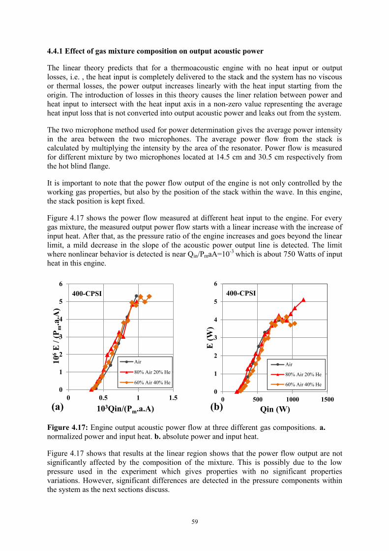
59
4.4.1 Effect of gas mixture composition on output acoustic power
The linear theory predicts that for a thermoacoustic engine with no heat input or output
losses, i.e. , the heat input is completely delivered to the stack and the system has no viscous
or thermal losses, the power output increases linearly with the heat input starting from the
origin. The introduction of losses in this theory causes the liner relation between power and
heat input to intersect with the heat input axis in a non-zero value representing the average
heat input loss that is not converted into output acoustic power and leaks out from the system.
The two microphone method used for power determination gives the average power intensity
in the area between the two microphones. The average power flow from the stack is
calculated by multiplying the intensity by the area of the resonator. Power flow is measured
for different mixture by two microphones located at 14.5 cm and 30.5 cm respectively from
the hot blind flange.
It is important to note that the power flow output of the engine is not only controlled by the
working gas properties, but also by the position of the stack within the wave. In this engine,
the stack position is kept fixed.
Figure 4.17 shows the power flow measured at different heat input to the engine. For every
gas mixture, the measured output power flow starts with a linear increase with the increase of
input heat. After that, as the pressure ratio of the engine increases and goes beyond the linear
limit, a mild decrease in the slope of the acoustic power output line is detected. The limit
where nonlinear behavior is detected is near Qin/PmaA=10-3
which is about 750 Watts of input
heat in this engine.
Figure 4.17: Engine output acoustic power flow at three different gas compositions. a.
normalized power and input heat. b. absolute power and input heat.
Figure 4.17 shows that results at the linear region shows that the power flow output are not
significantly affected by the composition of the mixture. This is possibly due to the low
pressure used in the experiment which gives properties with no significant properties
variations. However, significant differences are detected in the pressure components within
the system as the next sections discuss.
0
1
2
3
4
5
6
0 0.5 1 1.5
10
6 E
/ (
Pm
.a.A
)
103Qin/(Pm.a.A)
Air
80% Air 20% He
60% Air 40% He
400-CPSI
(a)
0
1
2
3
4
5
6
0 500 1000 1500
E (
W)
Qin (W)
Air
80% Air 20% He
60% Air 40% He
400-CPSI
(b)
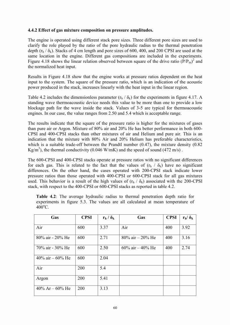
60
4.4.2 Effect of gas mixture composition on pressure amplitudes.
The engine is operated using different stack pore sizes. Three different pore sizes are used to
clarify the role played by the ratio of the pore hydraulic radius to the thermal penetration
depth (rh / δk). Stacks of 4 cm length and pore sizes of 600, 400, and 200 CPSI are used at the
same location in the engine. Different gas compositions are included in the experiments.
Figure 4.18 shows the linear relation observed between square of the drive ratio (P/Pm)2 and
the normalized heat input.
Results in Figure 4.18 show that the engine works at pressure ratios dependent on the heat
input to the system. The square of the pressure ratio, which is an indication of the acoustic
power produced in the stack, increases linearly with the heat input in the linear region.
Table 4.2 includes the dimensionless parameter (rh / δk) for the experiments in figure 4.17. A
standing wave thermoacoustic device needs this value to be more than one to provide a low
blockage path for the wave inside the stack. Values of 3-5 are typical for thermoacoustic
engines. In our case, the value ranges from 2.50 and 5.4 which is acceptable range.
The results indicate that the square of the pressure ratio is higher for the mixtures of gases
than pure air or Argon. Mixture of 80% air and 20% He has better performance in both 600-
CPSI and 400-CPSI stacks than other mixtures of air and Helium and pure air. This is an
indication that the mixture with 80% Air and 20% Helium has preferable characteristics,
which is a suitable trade-off between the Prandtl number (0.47), the mixture density (0.82
Kg/m3), the thermal conductivity (0.046 W/mK) and the speed of sound (472 m/s) .
The 600-CPSI and 400-CPSI stacks operate at pressure ratios with no significant differences
for each gas. This is related to the fact that the values of (rh / δk) have no significant
differences. On the other hand, the cases operated with 200-CPSI stack indicate lower
pressure ratios than those operated with 400-CPSI or 600-CPSI stack for all gas mixtures
used. This behavior is a result of the high values of (rh / δk) associated with the 200-CPSI
stack, with respect to the 400-CPSI or 600-CPSI stacks as reported in table 4.2.
Table 4.2: The average hydraulic radius to thermal penetration depth ratio for
experiments in figure 5.3. The values are all calculated at mean temperature of
400oC.
Gas CPSI rh / δk Gas CPSI rh/ δk
Air 600 3.37 Air 400 3.92
80% air - 20% He 600 2.71 80% air – 20% He 400 3.16
70% air - 30% He 600 2.50 60% air – 40% He 400 2.74
40% air – 60% He 600 2.04
Air 200 5.4
Argon 200 5.41
40% Ar – 60% He 200 3.13
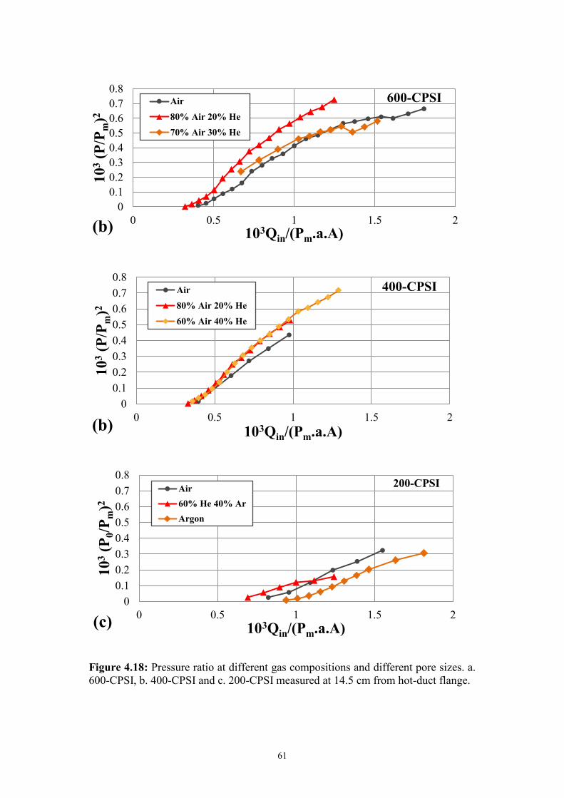
61
Figure 4.18: Pressure ratio at different gas compositions and different pore sizes. a.
600-CPSI, b. 400-CPSI and c. 200-CPSI measured at 14.5 cm from hot-duct flange.
0
0.1
0.2
0.3
0.4
0.5
0.6
0.7
0.8
0 0.5 1 1.5 2
10
3 (
P/P
m)2
103Qin/(Pm.a.A)
Air
80% Air 20% He
70% Air 30% He
600-CPSI
(b)
0
0.1
0.2
0.3
0.4
0.5
0.6
0.7
0.8
0 0.5 1 1.5 2
10
3 (
P/P
m)2
103Qin/(Pm.a.A)
Air
80% Air 20% He
60% Air 40% He
400-CPSI
(b)
0
0.1
0.2
0.3
0.4
0.5
0.6
0.7
0.8
0 0.5 1 1.5 2
10
3 (
P0/P
m)2
103Qin/(Pm.a.A)
Air
60% He 40% Ar
Argon
200-CPSI
(c)

62
4.4.3 Effect of gas mixture composition on harmonic distortion
The wave produced by the engine is a result of the addition of the fundamental wave to its
harmonics. The energy collection from the engine is usually through a single frequency
device. Therefore, the harmonics is regarded as a loss for the output acoustic power.
Figure 4.19: Normalized first harmonic amplitude versus normalized squared
fundamental amplitude at different gas compositions and different pore sizes. a. 600-
CPSI, b. 400-CPSI and c. 200-CPSI
0
0.2
0.4
0.6
0.8
0 2 4 6 8 10
10
3 (
P1/P
m)
103 (P0/Pm)2
Air, 600cpsi
80% Air 20% He, 600cpsi
70% Air 30% He, 600cpsi
a) 600-CPSI
(a)
0
0.2
0.4
0.6
0.8
0 2 4 6 8 10
10
3 (
P1/P
m)
103 (P0/Pm)2
Air, 400cpsi
80% Air 20% He, 400cpsi
60% Air 40% He, 400cpsi
b) 400-CPSI
(b)
0
0.2
0.4
0.6
0.8
0 2 4 6 8 10
10
3 (
P1/P
m)
103 (P0/Pm)2
Air, 200cpsi
60% He 40% Ar, 200cpsi
Argon, 200cpsi
c) 200-CPSI
(c)

63
The harmonic content is the most obvious nonlinear effect present in the present system. For
example, at the highest power recorded using 600-CPSI stack with air mixture, the amplitude
of the first harmonic P1 is 972 Pa, which is 0.378 of the amplitude of the fundamental of this
case, both measured using the same transducer at 14.5 cm from the hot-duct flange.
Figure 4.20 shows the relationship between the first harmonic pressure ratio to the square of
the fundamental pressure ratio for the same experiments in figure 4.19. Remarkably, the
results show that the relationship between the first harmonic and fundamental pressure ratios
is linear. The linear relationship for all experiments has nearly the same slope. The different
lines for different gas compositions and stack pore sizes start from the origin.
It can be concluded that the relationship is neither related significantly with the gas
composition nor the stack pore size. Whatever the source of P1 is, it is present and large. Its
thermoacoustic effect should be accounted for. It causes a DC flow and transports heat along
the stack. This requires a higher temperature difference between the two sides of the stack for
the same output acoustic power.
Figure 4.20: The linear behavior normalized first harmonic amplitude versus
normalized squared fundamental amplitude at different gas compositions and different
pore sizes.
Swift also suggests that the excess heat flow carried by P1 is expected to be nearly
proportional to P12
, and hence to P04, so that the excess acoustic power absorbed from the
fundamental must share this proportionality. The excess temperature difference needed
should therefore be proportional to P12, which is proportional to the input heat flow.
0
0.1
0.2
0.3
0.4
0.5
0.6
0.7
0.8
0.9
1
0 2 4 6 8 10
10
3 (
P1/P
m)
103 (P0/Pm)2
Air, 600cpsi 70% Air 30% He, 600cpsi Air, 400cpsi
80% Air 20% He, 400cpsi 60% Air 40% He, 400cpsi Air, 200cpsi
60% He 40% Ar, 200cpsi Argon, 200cpsi

64
This dependence is visible in figure 4.21. It shows that, while DELTAEC calculations show
that temperature difference increase is very low, the measurements showed a higher linear
increase in temperature difference, indicating that the excess temperature difference is
directly proportional to the input heat flow.
Figure 4.21: Temperature difference between the two sides of the stack versus the
heat input for different gas compositions and different pore sizes. a. 600-CPSI, b. 400-
CPSI and c. 200-CPSI compared to DELTAEC calculations for 100% air.
0
200
400
600
800
1000
0 200 400 600 800 1000 1200 1400
Td
iff (K
)
Qin (W)
Air, DeltaEC Air90% Air 10% He 80% Air 20% He70% Air 30% He
600-CPSI
(a)
0
200
400
600
800
1000
0 200 400 600 800 1000 1200 1400
Td
iff (K
)
Qin (W)
Air, DeltaEC 90% Air 10% He
80% Air 20% He 60% Air 40% He
400-CPSI
(b)
0
200
400
600
800
1000
0 200 400 600 800 1000 1200 1400
Td
iff (K
)
Qin (W)
Air, DeltaEC Air
60% He 40% Ar Argon
200-CPSI
(c)

65
4.5 Harmonic suppression
Despite its high environmental and simplicity advantages, the built thermoacoustic engine
presented in this work suffers high losses. One of the most obvious losses in the current
engine is the existence of harmonics.
Harmonic distortion of the resulting acoustic wave in a thermoacoustic engine is regarded a
loss. This is due to the fact that power generating devices from thermoacoustic engines, such
as linear alternator, work at a single frequency. Moreover, devices that can use the resulting
wave energy directly, such as in a thermoacoustically-driven thermoacoustic refrigerator, also
need to receive a single frequency. The power carried by higher order harmonics is therefore
lost as viscous heating in the air. Figure 4.22 shows that the power carried by the harmonic in
the system reaches 38.8% of the power carried by the fundamental wave which is rather a
significant loss.
Swift investigated the effect of adding inserts in the resonator on the first harmonic amplitude
(24). Placing an insert with lower flow area than the resonator at the velocity antinode of the
first harmonic resulted in decreasing its ratio to the fundamental amplitude. However, Swift
discussed neither the shape nor the blockage area or the thickness of these inserts.
The inserts are described in section 4.1.4. Every experiment is named as XYZ-N, where X is
the open insert area ratio (gas area/total resonator area), Y is the shape code: either A which
is a hollow ring, C which is multiple holes, or D which corresponds to DELTAEC
calculations. Z is the thickness of the insert in cm and N is the distance in cm between the
insert center and the hot-side blind flange. For example, the experiment 50C3-60 was done
using a stack which contains multiple holes, a stack open area of half the area of the resonator
area, a stack thickness of 3 cm, and the insert is placed 60 cm away from the blind flange.
Figure 4.22: power carried by the fundamental wave and the first harmonic for the 400-
CPSI stack operated with air as working fluid. Power measured using 2 microphones at
14.5cm and 59.5 cm from the hot-side blind flange.
4.5.1 Inserts effect on power and wave components
In this series of experiments, Inserts with various shapes and blockage areas are tested in the
resonator. All experiments are done with a 400-CPSI stack with air as working fluid. The
0
0.5
1
1.5
2
2.5
0 200 400 600 800 1000 1200 1400
Po
wer
(W
)
Qin (W)
Fundamental wave
First harmonic

66
stack center is placed at 5 cm away from the hot side flange. For every insert, the wave
components are studied and the acoustic power output is calculated. Calculations were done
using DELTAEC, modeling inserts as a duct which length is the stack thickness and has a
smaller area. This duct was placed in various places in the model. The model results indicate
the expected power, the expected frequency, and the fundamental dynamic pressure at the
same measurement location. As DELTAEC works at a single frequency, it is not possible to
obtain information about the harmonic content.
For every insert at a certain position, the voltage input to the heater is varied from 220V to
60V, which is equal to heat input ranging from 1680W to 125W. Figures 4.23 and 4.24 show
some notable results of the experiments. The first graph shows the acoustic power output
from the experiment sorted from higher to lower power output for different insert
configurations. The other graphs sort the columns according to the same order.
Figure 4.23: Power and frequency for multiple inserts with various shapes and positions. Solid
columns are measurements, hollow columns are DELTAEC calculations.
The results show the complexity of the parameters that control the power output. The
experiment named 0-0 is carried out with no insert placed in the resonator. It is seen that all
inserts of 50% and 75% open area resulted in power increase than the case with no insert.
DELTAEC predicted that inserts with 25% open area would result in higher power output.
This is due to that fact that DELTAEC does not take the non-linear losses of vortices and
flow restriction into account.
0
5
10
15
20
25D
1-6
2
50D
3-6
0
50D
3-6
2
50D
1-6
0
50D
1-6
2
75D
1-6
2
50C
3-6
0
50C
3-5
0
50C
1-6
2
50A
3-6
0
50C
3-6
2
50A
1-6
0
50C
1-6
0
50C
3-7
0
50A
1-6
2
50A
3-6
2
75A
1-6
2
50C
3-8
0
0-0
25A
1-6
2
25C
1-6
2
Po
wer
ma
x (
W)
a
175
180
185
190
195
200
25D
1-6
2
50D
3-6
0
50D
3-6
2
50D
1-6
0
50D
1-6
2
75D
1-6
2
50C
3-6
0
50C
3-5
0
50C
1-6
2
50A
3-6
0
50C
3-6
2
50A
1-6
0
50C
1-6
0
50C
3-7
0
50A
1-6
2
50A
3-6
2
75A
1-6
2
50C
3-8
0
0-0
25A
1-6
2
25C
1-6
2
Fre
qu
ency
(H
z)
b

67
The increase in the acoustic power that occurs in DELTAEC model results shows that the
insert does not only save the power lost in harmonics, but it also changes the acoustic
impedance of the resonator. The effect of this change in impedance on frequency is clearly
noticed in figure 4.23b. When frequency changes, the stack position in the wave changes and
the power output changes accordingly. DELTAEC results show that acoustic power output is
lower for the experiments with higher operating frequencies. This suggests that the change in
frequency changes the relative position of the fixed stack with respect to the acoustic wave,
resulting in a higher acoustic power output for the cases with lower frequencies.
Measurements confirms that result as the experiment with the highest operating frequency,
50C3-80, produced low acoustic power output compared to the same experiments that used
the 50C3 insert. Figure 5.24a shows the values of the fundamental pressure at the position of
the first microphone, 14.5 cm away from the hot side flange. This value is related to the
blockage that is present in the system due to the insert addition. For DELTAEC calculations,
the fundamental pressure at this location did not change significantly, ranging only from 5369
Pa to 5319 Pa.
Figure 4.24: Fundamental amplitude, and normalized ratio (Pm.P1/P02) for multiple inserts with
various shapes and positions. Solid columns are measurements, hollow columns are DELTAEC
calculations.
The measurements show that all the inserts caused the fundamental pressure to decrease due
to blockage, but the output acoustic power increased for some cases.
0
1000
2000
3000
4000
5000
6000
25D
1-6
2
50D
3-6
0
50D
3-6
2
50D
1-6
0
50D
1-6
2
75D
1-6
2
50C
3-6
0
50C
3-5
0
50C
1-6
2
50A
3-6
0
50C
3-6
2
50A
1-6
0
50C
1-6
0
50C
3-7
0
50A
1-6
2
50A
3-6
2
75A
1-6
2
50C
3-8
0
0-0
25A
1-6
2
25C
1-6
2
P0
,ma
x, m
ic1
(P
a)
a
0
1000
2000
3000
4000
5000
6000
50C
3-6
0
50C
3-5
0
50C
1-6
2
50A
3-6
0
50C
3-6
2
50A
1-6
0
50C
1-6
0
50C
3-7
0
50A
1-6
2
50A
3-6
2
75A
1-6
2
50C
3-8
0
0-0
25A
1-6
2
25C
1-6
2
(Pm
.P1/P
02)
b

68
Results shown in figure 4.24b present the ratio of the amplitude of the first harmonic and the
squared amplitude of the fundamental wave. Results show that it is maximum for the case of
no insert in the resonator. Cases that produce higher power output have a very low harmonic
content compared to the case with no insert. For example, the case that produced the highest
output power, 50C3-60, had a value for the quantity (Pm*P1/P02) of only 10% of the no-insert
case. The lowest harmonic content was 3.6% of the no insert case which was measured at the
50C3-50 case.
Figure 4.25: Power output and thermal to acoustic efficiency versus heat input to the system
with no insert in the resonator.
Figure 4.26: Power output and thermal to acoustic efficiency versus heat input to the system
with 50C3 is placed in the resonator 60 cm away from the hot-side flange.
The position of the insert 50C3 is changed inside the resonator. At every position, the heater
input is varied and the power and efficiency are calculated at every point. Figures 4.25 and
4.26 show the effect of varying the heat input to the system on efficiency and the acoustic
0
0.05
0.1
0.15
0.2
0.25
0.3
0.35
0.4
0.45
0.5
0.0
1.0
2.0
3.0
4.0
5.0
6.0
7.0
8.0
0.0 500.0 1000.0 1500.0 2000.0
Eff
icie
ncy
(%
)
pow
ero
ut (W
)
Qin (W)
Power_out
Efficiency
0.00
0.05
0.10
0.15
0.20
0.25
0.30
0.35
0.40
0.45
0.50
0.0
1.0
2.0
3.0
4.0
5.0
6.0
7.0
8.0
0.0 500.0 1000.0 1500.0 2000.0
Eff
icie
ncy
(%
)
po
wer
ou
t (W
)
Qin (W)
Power_out
Efficiency
50C3-60
No insert

69
power output values for the case of no insert and the case with the insert 50C3 located at 60
cm from the hot-side flange. The results also include the wave components which indicate the
fundamental and harmonic amplitudes. Power increases almost linearly with power input,
while efficiency has a maximum value of about 0.25% for no insert, and 0.46% for 50C3-60.
The relatively low efficiencies reported here are because the working gas is air at 1 bar.
Gases with larger sonic speed at higher pressures, like helium at 20 bars are typical in devices
of reasonable efficiencies, but related leakage problems arise.
4.5.2 Effect of insert position
The effect of the position, normalized with the wavelength, is shown in figure 4.27.
DELTAEC calculations, green points in figure 4.27a, show that the power output of the
system has a maximum value that occurs when the insert is located at about 0.32 of the
wavelength calculated from the hot-side flange. Measurements confirm these results, taking
the same trend but the powers are all scaled down about 40% due to non-linear losses that are
not accounted for on DELTAEC.
The fundamental pressure amplitude at the highest measured input power, 1680W, is shown
in figure 4.27b. Green dots show that fundamental pressure amplitude is not much affected by
the position of the insert in DELTAEC calculations, while measurements showed that the
pressure amplitude is less affected by blockage when the insert is closer to the cold side blind
flange. This suggests that the insertion of the flange nearer to the velocity antinode where the
velocity is meant to increase causes more vorticity and dissipates more energy.
Calculations of frequency using DELTAEC included in figure 5.17c, show that there is a
point with minimum frequency. These point are the same points that gave the model’s highest
power output, confirming the previously suggestions that the acoustic impedance changes and
makes the position of the stack closer to the optimum case in those positions in the linear
modeling. Measurements did not take the same trend. Measured frequency increases as the
distance from the hot-side flange increases.
Figure 4.27d shows the effect of the insert when placed at 62 cm from the hot-side flange on
the axial distribution of the first harmonic amplitude. It shows that the axial distribution
doesn’t change a lot when the insert is introduced. The location of the velocity antinode for
the first harmonic without the insert is at 62 cm from the hot-side flange. When the insert is
introduced, the position was not affected by this change.
The use of the DELTAEC model showed that the increase in power is not related only to
harmonic content reasons, but also occurs due to a change in the thermoacoustic
characteristics of the system.

70
Figure 4.27: Effect of normalized position of insert on selected parameters with 400cpsi stack. a)
Output power b) Fundamental pressure amplitude at 14.5 cm from hot-side blind flange c)
Frequency d) First harmonic amplitude along the resonator with and without the insert. Position
is the distance from hot-side flange.
0.0
2.0
4.0
6.0
8.0
10.0
12.0
14.0
0.25 0.30 0.35 0.40 0.45 0.50
Po
wer
ou
t (
W)
Insert position / wavelength
50C3
DeltaEC
a
0
1000
2000
3000
4000
5000
6000
0.25 0.30 0.35 0.40 0.45 0.50P
0 (
Pa
) Insert position / wavelength
50C3
DeltaEC
b
182
184
186
188
190
192
194
196
0.25 0.30 0.35 0.40 0.45 0.50
f (H
z)
Insert position / wavelength
50C3
DeltaEC
c
0
200
400
600
800
1000
1200
15 35 55 75
P (
Pa
)
Distance from Blind flange (cm)
50C3 at 62 cm
no insert
d

71
5. Conclusions and Suggestions for Future Work
5.1 Introduction
The present study aims to experimentally investigate the performance characteristics of a
thermoacoustic engine. A prototype of a standing-wave thermoacoustic engine was built in
the labs of the department of physics at The American University in Cairo. The engine was
operated using several gases and gas mixtures, stacks with different CPSI and different
operating conditions. Full runs of different running time were performed and data of
temperatures and dynamic pressure was collected to characterize the thermoacoustic engine
transient performance and to analyze the hysteresis of the acoustic power output. The
harmonic content of the wave is analyzed using a MATLAB code and related to the
temperature difference between the stack sides.
The engine was also operated at different constant heat inputs to analyze the steady state
performance and study the effect of gas mixture composition, stack CPSI, and heat input on
the operating frequency, acoustic power output and fundamental pressure amplitude of the
acoustic wave.
A numerical model of the engine is built using the DELTAEC software. The experimental
data is used to validate the results of the model. The model predicted the dynamic pressure
amplitude, volumetric velocity and the power flow inside the resonator. The code was also
used to investigate the performance of the engine at steady state. The predictions of the code
were significantly higher than the measurements.
The harmonic content of the output acoustic wave was analyzed at different heat input
different for several gases and gas mixtures. The effect of adding a flow semi-blocking insert
inside the resonator was investigated. Several inserts of different blockage areas and different
holes pattern were placed around the velocity antinode of the first harmonic to suppress it.
The effect of the insert on the losses related to the harmonic content is studied. The effect of
the insert thickness, position, shape and blockage area on the engine acoustic power output,
operating frequency, fundamental pressure amplitude, and suppression of the first harmonic
pressure amplitude is presented.
5.2 Conclusions of the present work
In view of what has been presented the following conclusions are drawn:
The prototype of the thermoacoustic engine produced a half-wavelength standing wave.
Measurements show that the acoustic power output increase linearly with the heat input for
low heat input. Working with air at atmospheric pressure using a 600-CPSI stack gives low
power density and therefore low efficiency. Higher acoustic power outputs can be obtained
by using mixtures of air and helium. A mixture of 80% air and 20% helium gives the highest
acoustic power and dynamic pressure at atmospheric pressure.
The numerical model of the engine gives accepted results for the resonance frequency.
However, the model calculations of the pressure and power agree only in trend with the
measured values. This may indicate that the model is not accurate for applications at
atmospheric mean pressure.

72
The mean temperature of the working gas filling the resonator is the critical parameter for the
hysteresis characteristics of the engine. At the same temperature difference, the dynamic
pressure amplitude during start-up and shut-down differs significantly for a longer running
time, lower helium content, lower starting temperature, or a stack of smaller pores.
Several inserts were used to suppress harmonics. All inserts of open area of 50% and 75% of
the resonator area increased the acoustic power output, while inserts with open area of 25%
of the resonator area caused high blockage and high losses and produced lower acoustic
power output. The insert with several holes with open area of 50% of the resonator area gave
the highest acoustic power output when placed at 0.32λ from the hot blind flange.
DELTAEC predicted that the thickness and the open area of the insert have a significant
effect on the acoustic power output. This suggests that the change is not only related to the
non-linear effect of the first harmonic which is not taken into account by DELTAEC, but also
due to the change of the wave shape inside the resonator. Specific inserts cause the stack to
be in a better position inside the resonator.
The position of the insert significantly affected the acoustic power output, the operating
frequency, and the fundamental pressure amplitude. An optimum position is at 0.32 of the
wavelength away from the hot-side blind flange.
5.3 Recommendations
More efforts are needed to reach a better understanding of the performance of thermoacoustic
engines. Further analysis of the hysteresis paths is needed to explain the main factors that
affect the phenomena. Harmonic content of the output acoustic wave need to be further
analysed.

73
References
(1) N. Rott, Thermoacoustics, Adv. Appl. Mech., 20:135-175 (1980).
(2) K.T. Feldman, Review of the literature on Rijke thermoacoustic phenomena, J. Sound
Vib. 7:83 (1968).
(3) N. Rott, Damped and thermally driven acoustic oscillations in wide and narrow tubes,
Zeitschrift für Angewandte Mathematik und Physik. 20:230 (1969).
(4) G.W. Swift, Thermoacoustic engines, J. Acoust. Soc. Am. 84:1146 (1988).
(5) N. Rott, Thermally driven acoustic oscillations, part II: Stability limit for helium, Z.
Angew. Math. Phys, 24:54 (1973)
(6) N. Rott, Thermally driven acoustic oscillations, part III: Second-order heat flux, Z.
Angew. Math. Phys., 26:43 (1975).
(7) N. Rott, Thermoacoustic heating at the closed end of an oscillating gas column, Fluid
Mech., 145:1(1984).
(8) M.E.H. Tijani, Loudspeaker-driven thermo-acoustic refrigeration, Ph.D. Thesis,
Technische Universiteit Eindhoven, (2001)
(9) H. Babaei and K Siddiqui, Design optimization of an automotive thermoacoustic air
refrigeration system, Acoustique Canadienne, 35:166-167 (2007).
(10) O. G. Symko, E. Abdel-Rahman, Y. S. Kwon, M. Emmi and R. Behunin, Design and
development of high-frequency thermoacoustic engines for thermal management of
microelectronics. Microelectron J. 35:185-191 (2004).
(11) M. Hatazawa , H. Sugita , T. Ogawa and Y. Seo, Performance of a thermoacoustic
sound wave generator driven with waste heat of automobile gasoline engine. Trans. Jpn.
Soc. Mech. Eng., 70:292-299 (2004).
(12) H. Babaei , K. Siddiqui and W. A. Chishty, Sustainable thermoacoustic refrigeration
system for gas turbine power plants, 17th symposium of industrial application of gas
turbines (IGAT); Banff, Canada (2007).
(13) L. Zoontjens, C. Howard, A. Zander and B. Cazzolate, Feasibility study of an
automotive thermoacoustic refrigerator. Proceedings of acoustics, Busselton, Australia,
(2005).
(14) R. L. Chen and S. L. Garrett, Solar/heat-driven thermoacoustic engine, J. Acoust. Soc.
Am., 103(5):2841 (1998).
(15) J. A. Adeff and T. J. Hofler, Design and construction of a solar powered
thermoacoustically driven thermoacoustic refrigerator, J. Acoust. Soc. Am., 107(6):L37-
42 (2000).
(16) R. Chen, Design, construction, and measurement of a larger Solar powered
thermoacoustic cooler, Pennsylvania State University (2001).

74
(17) C. Shen, Y. He , Y. Li, H. Ke, D. Zhang and Y. Liu, Performance of solar powered
thermoacoustic engine at different tilted angles, Applied Thermal Engineering, 29:2745-
2756 (2009).
(18) P. Merkli and H. Thomann, Thermoacoustic effect in a resonance tube, J. Fluid Mech.,
70:161 (1975).
(19) G.W. Swift, A unifying perspective for some engines and refrigerators, Acoustical
Society of America, Melville, (2002).
(20) N. M. Arafa, A. H. Ibrahim, K.Addas and Ehab Abdel-Rahman, Design considerations
for thermoacoustic engines for low onset temperature and efficient operation, Forum
Acusticum, Aalborg, Denmark (2011)
(21) J.R. Olson and G.W. Swift, Similitude in thermoacoustics, J. Acoust. Soc. Am.,
95:1405-1412 (1994).
(22) T. Jin, B. Zhang, K. Tang, R. Bao and G. Chen, Experimental observation on a small-
scale thermoacoustic prime mover. Journal of Zhejiang University, 8(2):205-209 (2007).
(23) G.W. Swift, Analysis and performance of a large thermoacoustic engine, J. Acoust. Soc.
Am. 92:1551-1563 (1992).
(24) A. H. Ibrahim and E. Abdel-Rahman, Innovative Solar-Energy-Driven Power
Converter: Efficient Operation of Thermo-acoustic Engines, The 2nd International
Conference on Renewable Energy: Generation and Applications, AlAin, UAE, 4 - 7
March, (2012).
(25) J. R. Belcher, W. V. Slaton, R. Raspet, H. E. Bass and J. Lightfoot Working gases in
thermo acoustic engines, J. Acoust. Soc. Am. 105 (5):2677-2684 (1999).
(26) W. C. Ward and G. W. Swift , Design environment for low-amplitude thermoacoustic
engines, J. Acoust. Soc. Am., 95(6):3671-3672 (1994).
(27) G. W. Swift, and W. C. Ward, Simple harmonic analysis of regenerators, J.
Thermophysics and Heat Transfer, 10:652-662 (1996).
(28) D. L. Gardner and G. W. Swift, A cascade thermoacoustic engine, J. Acoust. Soc. Am.
114(4):1905-1919 (2003).
(29) A. H. Ibrahim, N. M. Arafa and E. E. Khalil, Geometrical optimization of
thermoacoustic heat engines. 49th AIAA Aerospace Sciences Meeting. AIAA 2011-129,
Orlando, Florida (2011).
(30) N. M. Arafa, A. H. Ibrahim and E.E. Khalil, Sensitivity analysis of a standing-wave
thermoacoustic engine, 9th Annual International Energy Conversion Engineering
Conference, AIAA 2011, San Diego, California, (2011).
(31) H. Babaei and K. Siddiqui, Design and optimization of thermoacoustic devices, Energy
Conversion and Management, 49:3585-3598 (2008).
(32) M. Wetzel, Experimental investigation of a single plate thermoacoustic refrigerators,
Ph.D. thesis, Johns Hopkins University (1998).

75
(33) E. Besnoin, Numerical study of thermoacoustic heat exchangers, Ph.D. thesis, Johns
Hopkins University (2001).
(34) L. Zoontjens, C.Q. Howard, A.C. Zander and B.S. Cazzolato, Modeling and optimization
of acoustic inertance segments for thermoacoustic devices, Proceedings of Acoustics,
435-441 (2006).
(35) Y. Ueda, T. Biwa, U. Mizutani and T. Yazaki, Experimental studies of a thermoacoustic
Stirling prime mover and its application to a cooler, J. Acoust. Soc. Am., 72 (3):1134-
1141 (2003).
(36) M.E.H. Tijani, J.C.H. Zeegers and A.T.A.M. de Waele, Design of thermoacoustic
refrigerators, Cryogenics 42:49-57 (2002).
(37) S. Backhaus and G.W. Swift, A thermoacoustic stirling heat engine: detailed study, J.
Acoust. Soc. Am.,107:3148-3166 (2000).
(38) M.E. Poesse and S.L. Garrett, Performance measurements on a thermoacoustic
refrigerator driven at high amplitudes, J. Acoust. Soc. Am., 107:2480-2486 (2000).
(39) J. Lighthill, Acoustic streaming, J. Sound and Vibration 61:391-418 (1978).
(40) W.L.M. Nyborg, Physical Acoustics, Vol. IIB, New York, (1965).
(41) M. Watanabe, A. Prosperetti and H. Yuan, A simple model for linear and nonlinear
processes in thermoacoustic prime movers, Part I: Model and linear theory, J. Acoust.
Soc. Am., 102(6):3484-3496 (1997).
(42) H. Yuan, S. Karpov and A. Prosperetti, A simple model for linear and nonlinear
processes in thermoacoustic prime movers, Part II: Nonlinear oscillations, J. Acoust.
Soc. Am., 102(6):3497-3506 (1997).
(43) S. Karpov, A. Prosperetti, Nonlinear saturation of the thermoacoustic instability, J.
Acoust. Soc. Am., 107(6):3130-3147 (2000).
(44) M. F. Hamilton, Y. A. Ilinski and F. A. Zabolotskaya, Nonlinear two-dimensional model
for thermoacoustic engines, J. Acoust. Soc. Am., 111(5): 2076-2086 (2002).
(45) B. L. Smith and G. W. Swift, Measuring second-order time-average pressure, J. Acoust.
Soc. Am., 110:717-723 (2001).
(46) A.A. Atchley, H.E. Bass, and T. Hofler, Frontiers of nonlinear acoustics, Elsevier
Science Publishers, London, 603-608 (1990).
(47) D.F. Gaitan and A. Atchley, Finite amplitude standing waves in harmonic and
anharmonic tubes, J. Acoust. Soc. Am. 93:2489–2495 (1993).
(48) P.H.M.W Panhuis, Mathematical aspects of thermoacoustics. Eindhoven: TUE:
Department of Mathematics and Computer Science (2009).
(49) P.C.H. Aben, P.R. Bloemen, and J.C.H. Zeegers, 2-D PIV measurements of oscillatory
flow around parallel plates, Experiments in Fluids (2008).
76
(50) P. Merkli and H. Thomann, Transition to turbulence in oscillating pipe-flow, J. of Fluid
Mechanics, 68:567–575 (1975).
(51) D.L. Gardner, J.R. Olson, and G.W. Swift, Turbulent losses in thermoacoustic
resonators, J. Acoust. Soc. Am., 98:2961 (1995).
(52) A. H. Ibrahim, A. Elbeltagy, M. Emam and E. Abdel-Rahman, Development and
analysis of non-linearity in the pressure waves resulting from thermoacoustic heat
engines, Acoustics 2012, Nantes, France, (2012).
(53) S. Backhaus and G. W. Swift, A thermoacoustic Stirling heat engine. Nature; 399:335–
338 (1999).
(54) S. L. Garrett and S. Backhaus, The power of sound, American scientist, 88:516 (2000).
(55) T. Valdes-Solis, G. Marban and A.B. Fuertes, Preparation of microporous carbon-
ceramic cellular monoliths, Microporous and Mesoporous Materials, 113-126 43(2001).
(56) T. Biwa, Y. Tashiro, H. Nomura, Y. Ueda, and T. Yazaki, Experimental verification of
two-sensor acoustic intensity measurements in lossy ducts, J. Acoust. Soc. Am.,
124(3):1584-1590 (2008).
(57) S. Backhaus, G. W. Swift, and R. S. Reid, High-temperature self-circulating
thermoacoustic heat exchanger, Applied Physics Letters, 87 (2005).
(58) A. T. A. M. De Waele, Basic treatment of onset conditions and transient effects in
thermoacoustic Stirling engines, Journal of Sound and Vibration, 325(4):974-988 (2009).
(59) A.H. Ibrahim, M. Emam, Hosny Omar, K. Addas and E. Abdel-Rahman, Performance
evaluation of thermoacoustic engine using different gases, Proceedings of ICSV19,
Vilnius, Lithuania (2012).

77
Appendix A: Properties of working gas mixture
Table A : Thermal properties of air-He mixtures used in experiments
Air
Fraction
Mixture
Density
Kinematic
Viscosity
Thermal
Conductivity
Heat
Capacity
Prandtl
number Gamma Mole
Kg/m3 m
2/s J.m
-1K
-1s
-1 J.Kg
-1K
-1 Kg/Kmole
1.0 0.993 2.11E-05 0.030 1014 0.711 1.394 29
0.9 0.908 2.34E-05 0.036 1070 0.642 1.411 26.5
0.8 0.822 2.61E-05 0.042 1154 0.589 1.429 24
0.6 0.651 3.40E-05 0.058 1367 0.518 1.471 19
0.4 0.480 4.73E-05 0.081 1732 0.485 1.521 14
0.2 0.309 7.45E-05 0.115 2503 0.501 1.585 9
0.0 0.138 1.59E-04 0.170 5193 0.667 1.667 4

Appendix B: DELTAEC code
ENGINE 5 inch.out
!Created with DeltaEC version 6.3b11.12!under win32,
using Win 6.1.7601 (Service Pack 1) under Python DeltaEC.
!--------------------------------- 0 ---------------------------------
BEGIN Global Variables
1.0000E+05 a Mean P Pa
202.50 b Freq Hz G
325.00 c TBeg K
1.8005E+04 d |p| Pa G
0.0000 e Ph(p) deg
0.0000 f |U| m^3/s
0.0000 g Ph(U) deg
air Gas type
!--------------------------------- 1 ---------------------------------
DUCT Resonator
1.2661E-02 a Area m^2 Mstr 5362.4 A |p| Pa
0.39888 b Perim m 1a 0.96877 B Ph(p) deg
0.3600 c Length m 0.56247 C |U| m^3/s
5.0000E-02 d Srough -90.009 D Ph(U) deg
0.0000 E Htot W
ideal Solid type -25.732 F Edot W
!--------------------------------- 2 ---------------------------------
DUCT Insert
1.2661E-02 a Area m^2 Mstr 3513.8 A |p| Pa
0.39888 b Perim m 2a 1.5561 B Ph(p) deg
3.0000E-02 c Length m 0.57782 C |U| m^3/s
5.0000E-04 d Srough -89.979 D Ph(U) deg
0.0000 E Htot W
ideal Solid type -27.19 F Edot W
!--------------------------------- 3 ---------------------------------
DUCT Resonator
1.2661E-02 a Area m^2 Mstr 4040.9 A |p| Pa
0.39888 b Perim m 3a 177.90 B Ph(p) deg
0.1200 c Length m 0.57414 C |U| m^3/s
5.0000E-02 d Srough -89.806 D Ph(U) deg
0.0000 E Htot W
ideal Solid type -46.521 F Edot W
!--------------------------------- 4 ---------------------------------
SURFACE MIC 2
0.0000 a Area m^2 4040.9 A |p| Pa

177.90 B Ph(p) deg
0.57414 C |U| m^3/s
-89.806 D Ph(U) deg
0.0000 E Htot W
ideal Solid type -46.521 F Edot W
!--------------------------------- 5 ---------------------------------
DUCT between mics
1.2661E-02 a Area m^2 Mstr 1.2785E+04 A |p| Pa
0.39888 b Perim m 5a 179.32 B Ph(p) deg
0.1600 c Length m 0.41453 C |U| m^3/s
5.0000E-02 d Srough -89.249 D Ph(U) deg
0.0000 E Htot W
ideal Solid type -66.256 F Edot W
!--------------------------------- 6 ---------------------------------
SURFACE MIC 1
0.0000 a Area m^2 1.2785E+04 A |p| Pa
179.32 B Ph(p) deg
0.41453 C |U| m^3/s
-89.249 D Ph(U) deg
0.0000 E Htot W
ideal Solid type -66.256 F Edot W
!--------------------------------- 7 ---------------------------------
DUCT before mic 1
1.2661E-02 a Area m^2 Mstr 1.7072E+04 A |p| Pa
0.39888 b Perim m 7a 179.74 B Ph(p) deg
0.1300 c Length m 0.1869 C |U| m^3/s
5.0000E-02 d Srough -87.631 D Ph(U) deg
0.0000 E Htot W
ideal Solid type -73.283 F Edot W
!--------------------------------- 8 ---------------------------------
HX Ambient HX
1.2661E-02 a Area m^2 1.7320E+04 A |p| Pa
0.9000 b GasA/A 179.61 B Ph(p) deg
1.0000E-02 c Length m 0.16772 C |U| m^3/s
sameas 10d d y0 m -86.799 D Ph(U) deg
-1680.0 e HeatIn W -1680.0 E Htot W
500.00 f SolidT K -91.106 F Edot W
325.00 G GasT K
copper Solid type 274.05 H SolidT K
!--------------------------------- 9 ---------------------------------
RPN ChangeMe
0.0000 a G or T 1680.0 A ChngeMe
8e ~

!--------------------------------- 10 ---------------------------------
STKRECT Ceramic stack
1.2661E-02 a Area m^2 1.7936E+04 A |p| Pa
0.85866 b GasA/A 10def 178.62 B Ph(p) deg
3.0000E-02 c Length m 0.1259 C |U| m^3/s
4.8000E-04 d aa m Mstr -92.751 D Ph(U) deg
3.8000E-05 e Lplate m Mstr -1680.0 E Htot W
sameas 10d f bb m Mstr 26.956 F Edot W
325.00 G TBeg K
celcor Solid type 499.37 H TEnd K
!--------------------------------- 11 ---------------------------------
HX Hot Hex
1.2661E-02 a Area m^2 1.8042E+04 A |p| Pa
0.9000 b GasA/A 178.49 B Ph(p) deg
1.0000E-02 c Length m 0.10471 C |U| m^3/s
sameas 10d d y0 m -91.621 D Ph(U) deg
sameas 9A e HeatIn W 0.0000 E Htot W
300.00 f SolidT K 1.8243 F Edot W
499.37 G GasT K
copper Solid type 552.13 H SolidT K
!--------------------------------- 12 ---------------------------------
DUCT Change Me
sameas 7a a Area m^2 1.8227E+04 A |p| Pa
0.39888 b Perim m 178.49 B Ph(p) deg
5.0000E-02 c Length m 3.2732E-12 C |U| m^3/s
5.0000E-04 d Srough 69.359 D Ph(U) deg
0.0000 E Htot W
ideal Solid type -9.7738E-09 F Edot W
!--------------------------------- 13 ---------------------------------
HARDEND target this to seal the end
0.0000 a R(1/z) =13G 1.8227E+04 A |p| Pa
0.0000 b I(1/z) =13H 178.49 B Ph(p) deg
0.0000 c Htot W 3.2732E-12 C |U| m^3/s
69.359 D Ph(U) deg
0.0000 E Htot W
-9.7738E-09 F Edot W
-1.4524E-12 G R(1/z)
-4.1879E-12 H I(1/z)
!--------------------------------- 14 ---------------------------------
RPN Effeciency Calculations
0.0000 a G or T 4.3621E-02 A etaI
0.34918 B EtaC
0.12493 C etaII

3.1913 D 2y/dk
174.37 E Tdiff
10H 10G - 10d 2 * dk / 7F ~ 11e / 10H 10G - 10H / / 10H 10G - 10H / 7F ~
11e /
! The restart information below was generated by a previous run
! and will be used by DeltaEC the next time it opens this file.
guessz 0b 0d
xprecn 3.3414E-03 1.8656E-02
targs 13a 13b
mstr-slave 6 1 -2 2 -2 3 -2 5 -2 7 -2 10 -1
! Plot start, end, and step values. May be edited if you wish.
! Outer Loop: | Inner Loop

دراسات عملية حول أداء المحركات الحرارية الصوتية ذات األمواج الموقوفة
إعداد
محمود محمد إمام رجب مهندس/
كليــة الهندســة ، جامعــة القاهــرة
الجيـزة ، جمهوريـة مصـر العربيــة
3102
رسالة مقدمة إلى كلية الهندسة، جامعة القاهرة
كجزء من متطلبات الحصول على درجة
الماجستير
في هندسة القوى الميكانيكية

دراسات عملية حول أداء المحركات الحرارية الصوتية ذات األمواج الموقوفة
إعداد
محمود محمد إمام رجب مهندس/
تحت إشـــراف
كليــة الهندســة ، جامعــة القاهــرة
الجيـزة ، جمهوريـة مصـر العربيــة
0231
رسالة مقدمة إلى كلية الهندسة، جامعة القاهرة
الحصول على درجةكجزء من متطلبات
الماجستير
في هندسة القوى الميكانيكية
محمود أحمد فؤاداألستاذ الدكتور/
قسم القوى الميكذنيكيةب تساذ األ
جذمعة القذهرةكلية الهندتسة،
إيهاب عبدالرحمنالدكتور/
الفيزيذء بقسمالمسذعد تساذ األ
كلية العلوم والهندتسة، الجذمعة األمريكية بذلقذهرة
عبدالماجد ابراهيم العيسويالدكتور/
المدرس بقسم القوى الميكذنيكية
جذمعة القذهرة كلية الهندتسة،

دراسات عملية حول أداء المحركات الحرارية الصوتية ذات األمواج الموقوفة
إعداد
محمود محمد إمام رجب مهندس/
محمود عبدالفتاح القاضي/ األتساذ الدكاور عضو
عصام الدين خليل حسن األتساذ الدكاور/ عضو
مشرف ، و عضو
اللجنة فؤادمحمود أحمد / األتساذ الدكاور
كليــة الهندســة ، جامعــة القاهــرة
الجيـزة ، جمهوريـة مصـر العربيــة
0231
القاهرةرسالة مقدمة إلى كلية الهندسة، جامعة
كجزء من متطلبات الحصول على درجة
الماجستير
في هندسة القوى الميكانيكية
:يعتمد من لجنة الممتحنين

محمود محمد إمذم رجب االسم:
10/10/0191 : تاريخ الميالد
مصري الجنسية:
[email protected] البريد االلكتروني:
01111238133 التليفون:
القنذطر الخيرية، القليوبية، مصر العنوان:
2010/ 10/ 01 تاريخ التسجيل:
/ / تاريخ منح الدرجة:
مذجساير العلوم الهندتسية الدرجة:
هندتسة القوى الميكذنيكية القسم:
المشرفين: )المشرف الرئيسي( أ.د. محمود أحمد فؤاد
عبدالرحمند. إيهذب
د. عبدالمذجد ابراهيم عيسوي
الممتحنين:
)مماحن خذرجي( أ.د. محمود عبدالفاذح القذضي
)مماحن داخلي( عصذم الدين خليل حسن خليل أ.د.
)عن المشرفين( أ.د. محمود أحمد فؤاد
الصوتية ذات األمواج الموقوفةدراسات عملية حول أداء المحركات الحرارية عنوان الرسالة:
محركذت حرارية صوت طذقة قدرة ماجددة غذزات نبيلة تبذين تردد :الكلمات المفتاحية
الملخص:
تساهدف هذه الدراتسة الاعرف على بعض مالمح أداء المرحذت الصوتية الحرارية بذتساخدام غذزات
فة. يام دراتسة األداء خالل الاشغيل مخالفة وعنذصر مصدرة للصوت ات فاحذت مربعة بمقذتسذت مخال
فذعلية اضذفة عوائق في وتفحص الدراتسة المسامر الثذبت، وأثنذء الدورات الكذملة من تشغيل وإطفذء.
مسذر الموجة لاقليل الفقد في الطذقة في الارددات العذلية. تظهر الناذئج أن مزيجذ من الهواء والهليوم
ط الجوي. وتاضح ظذهرة الابذينية في الدورات الطويلة وتظهر يعطي ناذئج أفضل من الهواء في الضغ
الناذئج اعامذدهذ على نوعية الغذز ووقت الاشغيل ونوع العنصر المصدر للصوت. تظهر الدراتسة
فذعلية العوائق في تقليل الفقد في الطذقة الذي تسببه الارددات المخالفة عن الاردد الرئيسي.

ملخص البحث
المحركات الحرارية الصوتية من النظم الحديثة لتحويل طاقة الحرارة إلى شغل مفيد على هيئة
أمواج صوتية. يستهدف هذا العمل البحثي توضيح بعض الخصائص التي تظهر في أثناء التشغيل
مختلفة وتحت الضغط الجوي، في حالتي المستمر لمحرك حراري صوتي ذي موجة موقوفة بغازات
التشغيل المنتظم، ودورات التشغيل الكاملة؛ التي تشمل قيام المحرك وانتظام حالته ثم إيقافه. تظهر
النتائج أن أداء المحرك يتأثر بطريقة كبيرة بنوعية الغاز المستخدم، ونفاذية المكون الفعال، وكمية
شغيل المنتظم، تظهر آثار هذه العوامل على الطاقة الصوتية الناتجة، الحرارة النافذة إلى المحرك. في الت
وعلى الضغط الديناميكي التي تحمله الموجة الصوتية الموقوفة الناتجة، وعلى التشوه الهرموني الذي
يظهر في األمواج. ويظهر تأثير العوامل سابقة الذكر في أثناء دورات التشغيل الكاملة على تطور
التي تظهر تغير Hysteresis ترددي للموجة مع تغير درجة الحرارة، وعلى ظاهرة التباينيةالمحتوى ال
مسارات الضغط في أثناء تزايد درجة الحرارة عنها أثناء تناقصها. يستهدف العمل أيضا التحقق من
يل فاعلية وضع عوائق خاصة في مسار األمواج الصوتية الموقوفة لتحسين محتواها الهرموني وتقل
تشوهه لتقليل فقد الطاقة. وتدرس النتائج تأثير مكان وشكل ومساحة العوائق على األداء. تظهر النتائج
فاعلية كبيرة لهذه الطريقة التي ضاعفت الطاقة الصوتية الناتجة في بعض الحاالت رغم تقليل نسبة
ون نتاجا خالصا لتحسن الضغط الديناميكي الناتجة، إال أن النتائج توضح أن هذا التحسن قد ال يك
الخصائص الهرمونية للموجة، وإنما قد تكون العوائق تسببت في تغييرات في التردد والمكان النسبي
في مسار الموجة الموقوفة. Stackللمكون المنتج للطاقة