Excel 2007 PivotTables - dbmanagement.infodbmanagement.info/Books/Others/Excel_2007_PivotTables_Recipes.pdf · Excel 2007 PivotTables Recipes: A Problem-Solution Approach ... Preparing

Debra Dalgleish

Excel 2007 PivotTables RecipesA Problem-Solution Approach

Excel 2007 PivotTables Recipes: A Problem-Solution Approach

Copyright © 2007 by Debra Dalgleish

All rights reserved. No part of this work may be reproduced or transmitted in any form or by any means,electronic or mechanical, including photocopying, recording, or by any information storage or retrievalsystem, without the prior written permission of the copyright owner and the publisher.

ISBN-13 (pbk): 978-1-59059-920-4

ISBN-10 (pbk): 1-59059-920-9

Printed and bound in the United States of America 9 8 7 6 5 4 3 2 1

Trademarked names may appear in this book. Rather than use a trademark symbol with every occurrenceof a trademarked name, we use the names only in an editorial fashion and to the benefit of the trademarkowner, with no intention of infringement of the trademark.

Lead Editor: Tom WelshTechnical Reviewer: Roger GovierEditorial Board: Steve Anglin, Ewan Buckingham, Tony Campbell, Gary Cornell, Jonathan Gennick,

Jason Gilmore, Kevin Goff, Jonathan Hassell, Matthew Moodie, Joseph Ottinger, Jeffrey Pepper, Ben Renow-Clarke, Dominic Shakeshaft, Matt Wade, Tom Welsh

Project Manager: Beth ChristmasCopy Editor: Marcia BakerAssociate Production Director: Kari Brooks-CoponyProduction Editor: Katie StenceCompositor: Linda Weidemann, Wolf Creek PressProofreader: Liz WelchIndexer: Brenda MillerArtist: April MilneCover Designer: Kurt KramesManufacturing Director: Tom Debolski

Distributed to the book trade worldwide by Springer-Verlag New York, Inc., 233 Spring Street, 6th Floor,New York, NY 10013. Phone 1-800-SPRINGER, fax 201-348-4505, e-mail [email protected],or visit http://www.springeronline.com.

For information on translations, please contact Apress directly at 2855 Telegraph Avenue, Suite 600,Berkeley, CA 94705. Phone 510-549-5930, fax 510-549-5939, e-mail [email protected], or visithttp://www.apress.com.

The information in this book is distributed on an “as is” basis, without warranty. Although every pre-caution has been taken in the preparation of this work, neither the author(s) nor Apress shall have anyliability to any person or entity with respect to any loss or damage caused or alleged to be caused directlyor indirectly by the information contained in this work.

The source code for this book is available to readers at http://www.apress.com.

Contents at a Glance

About the Author . . . . . . . . . . . . . . . . . . . . . . . . . . . . . . . . . . . . . . . . . . . . . . . . . . . . . . . . . . . . . . . . . xiii

About the Technical Reviewer. . . . . . . . . . . . . . . . . . . . . . . . . . . . . . . . . . . . . . . . . . . . . . . . . . . . . . . xv

Acknowledgments . . . . . . . . . . . . . . . . . . . . . . . . . . . . . . . . . . . . . . . . . . . . . . . . . . . . . . . . . . . . . . . xvii

Introduction. . . . . . . . . . . . . . . . . . . . . . . . . . . . . . . . . . . . . . . . . . . . . . . . . . . . . . . . . . . . . . . . . . . . . . xix

■CHAPTER 1 Creating a Pivot Table . . . . . . . . . . . . . . . . . . . . . . . . . . . . . . . . . . . . . . . . . . 1

■CHAPTER 2 Sorting and Filtering Pivot Table Data . . . . . . . . . . . . . . . . . . . . . . . . . . 21

■CHAPTER 3 Calculations in a Pivot Table . . . . . . . . . . . . . . . . . . . . . . . . . . . . . . . . . . . 41

■CHAPTER 4 Formatting a Pivot Table . . . . . . . . . . . . . . . . . . . . . . . . . . . . . . . . . . . . . . . 71

■CHAPTER 5 Grouping and Totaling Pivot Table Data. . . . . . . . . . . . . . . . . . . . . . . . 101

■CHAPTER 6 Modifying a Pivot Table . . . . . . . . . . . . . . . . . . . . . . . . . . . . . . . . . . . . . . . 123

■CHAPTER 7 Updating a Pivot Table . . . . . . . . . . . . . . . . . . . . . . . . . . . . . . . . . . . . . . . . 139

■CHAPTER 8 Pivot Table Security, Limits, and Performance . . . . . . . . . . . . . . . . . 155

■CHAPTER 9 Printing and Extracting Pivot Table Data . . . . . . . . . . . . . . . . . . . . . . . 167

■CHAPTER 10 Pivot Charts . . . . . . . . . . . . . . . . . . . . . . . . . . . . . . . . . . . . . . . . . . . . . . . . . . 189

■CHAPTER 11 Programming a Pivot Table . . . . . . . . . . . . . . . . . . . . . . . . . . . . . . . . . . . 205

■INDEX . . . . . . . . . . . . . . . . . . . . . . . . . . . . . . . . . . . . . . . . . . . . . . . . . . . . . . . . . . . . . . . . . . . . . . . 237

iii

Contents

About the Author . . . . . . . . . . . . . . . . . . . . . . . . . . . . . . . . . . . . . . . . . . . . . . . . . . . . . . . . . . . . . . . . . xiii

About the Technical Reviewer. . . . . . . . . . . . . . . . . . . . . . . . . . . . . . . . . . . . . . . . . . . . . . . . . . . . . . . xv

Acknowledgments . . . . . . . . . . . . . . . . . . . . . . . . . . . . . . . . . . . . . . . . . . . . . . . . . . . . . . . . . . . . . . . xvii

Introduction. . . . . . . . . . . . . . . . . . . . . . . . . . . . . . . . . . . . . . . . . . . . . . . . . . . . . . . . . . . . . . . . . . . . . . xix

■CHAPTER 1 Creating a Pivot Table . . . . . . . . . . . . . . . . . . . . . . . . . . . . . . . . . . . . . . . 1

1.1. Planning a Pivot Table: Getting Started . . . . . . . . . . . . . . . . . . . . . 1

1.2. Planning a Shared Pivot Table. . . . . . . . . . . . . . . . . . . . . . . . . . . . . 2

1.3. Preparing the Source Data: Using Excel Data. . . . . . . . . . . . . . . . 4

1.4. Preparing the Source Data: Creating an Excel Table. . . . . . . . . . 6

1.5. Preparing the Source Data: Excel Field Names Not Valid . . . . . . 8

1.6. Preparing the Source Data: Using Filtered Excel Data . . . . . . . . 8

1.7. Preparing the Source Data: Using an Excel Table with Monthly Columns . . . . . . . . . . . . . . . . . . . . . . . . . . . . . . . . . . . . . 9

1.8. Preparing the Source Data: Using an Access Query . . . . . . . . . 13

1.9. Preparing the Source Data: Using a Text File . . . . . . . . . . . . . . . 14

1.10. Preparing the Source Data: Using an OLAP Cube . . . . . . . . . . 14

1.11. Creating the Pivot Table: Using Excel Data as the Source . . . . . . . . . . . . . . . . . . . . . . . . . . . . . . . . . . . . . . . . . . . . . 15

1.12. Creating the Pivot Table: Using Excel Data on Separate Sheets . . . . . . . . . . . . . . . . . . . . . . . . . . . . . . . . . . . . . . . . 15

1.13. Creating the Pivot Table: Using the PivotTable Field List. . . . . . . . . . . . . . . . . . . . . . . . . . . . . . . . . . . . . . . . . . . . . . . . 18

1.14. Creating the Pivot Table: Changing the Field List Order . . . . . . . . . . . . . . . . . . . . . . . . . . . . . . . . . . . . . . . . . . . . . . . 20

■CHAPTER 2 Sorting and Filtering Pivot Table Data . . . . . . . . . . . . . . . . . . . . . 21

2.1. Sorting a Pivot Field: Sorting Row Labels . . . . . . . . . . . . . . . . . . 21

2.2. Sorting a Pivot Field: New Items Out of Order . . . . . . . . . . . . . . 23

2.3. Sorting a Pivot Field: Sorting Items Left to Right . . . . . . . . . . . 24

2.4. Sorting a Pivot Field: Sorting Items in a Custom Order . . . . . . . 25

2.5. Sorting a Pivot Field: Items Won’t Sort Correctly . . . . . . . . . . . . 27

2.6. Filtering a Pivot Field: Filtering Row Label Text. . . . . . . . . . . . . . 28v

2.7. Filtering a Pivot Field: Applying Multiple Filters to a Field . . . . 29

2.8. Filtering a Pivot Field: Filtering Row Label Dates . . . . . . . . . . . . 31

2.9. Filtering a Pivot Field: Filtering Values for Row Fields. . . . . . . . 32

2.10. Filtering a Pivot Field: Filtering for Nonconsecutive Dates . . . . . . . . . . . . . . . . . . . . . . . . . . . . . . . . . . . . 33

2.11. Filtering a Pivot Field: Including New Items in a Manual Filter . . . . . . . . . . . . . . . . . . . . . . . . . . . . . . . . . . . . . . . . . . . . 34

2.12. Filtering a Pivot Field: Filtering by Selection. . . . . . . . . . . . . . . 35

2.13. Filtering a Pivot Field: Filtering for Top Items . . . . . . . . . . . . . . 36

2.14. Using Report Filters: Hiding Report Filter Items . . . . . . . . . . . . 37

2.15. Using Report Filters: Filtering for a Date Range . . . . . . . . . . . . 38

2.16. Using Report Filters: Filtering for Future Dates . . . . . . . . . . . . 38

■CHAPTER 3 Calculations in a Pivot Table . . . . . . . . . . . . . . . . . . . . . . . . . . . . . . . 41

3.1. Using Summary Functions: Defaulting to Sum or Count. . . . . . 41

3.2. Using Summary Functions: Counting Blank Cells . . . . . . . . . . . 45

3.3. Using Custom Calculations: Difference From . . . . . . . . . . . . . . . 46

3.4. Using Custom Calculations: % Of . . . . . . . . . . . . . . . . . . . . . . . . 48

3.5. Using Custom Calculations: % Difference From . . . . . . . . . . . . 49

3.6. Using Custom Calculations: Running Total . . . . . . . . . . . . . . . . . 50

3.7. Using Custom Calculations: % of Row. . . . . . . . . . . . . . . . . . . . . 52

3.8. Using Custom Calculations: % of Column . . . . . . . . . . . . . . . . . . 53

3.9. Using Custom Calculations: % of Total . . . . . . . . . . . . . . . . . . . . 54

3.10. Using Custom Calculations: Index . . . . . . . . . . . . . . . . . . . . . . . 55

3.11. Using Formulas: Calculated Field vs. Calculated Item . . . . . . 56

3.12. Using Formulas: Adding Items With a Calculated Item . . . . . . 57

3.13. Using Formulas: Modifying a Calculated Item . . . . . . . . . . . . . 58

3.14. Using Formulas: Removing a Calculated Item . . . . . . . . . . . . . 59

3.15. Using Formulas: Using Index Numbers in a Calculated Item . . . . . . . . . . . . . . . . . . . . . . . . . . . . . . . . . . . . . . . . . . 59

3.16. Using Formulas: Modifying a Calculated Item Formula in Cell . . . . . . . . . . . . . . . . . . . . . . . . . . . . . . . . . . . . . . . . . . . . . . . . . . 60

3.17. Using Formulas: Creating a Calculated Field . . . . . . . . . . . . . . 61

3.18. Using Formulas: Modifying a Calculated Field . . . . . . . . . . . . . 62

3.19. Using Formulas: Removing a Calculated Field . . . . . . . . . . . . . 63

3.20. Using Formulas: Determining the Type of Formula . . . . . . . . . 63

3.21. Using Formulas: Adding a Calculated Item to a Field with Grouped Items . . . . . . . . . . . . . . . . . . . . . . . . . . . . . . . . . . . . . . 64

3.22. Using Formulas: Calculating the Difference Between Amounts. . . . . . . . . . . . . . . . . . . . . . . . . . . . . . . . . . . . . . . . 64

■CONTENTSvi

3.23. Using Formulas: Correcting the Grand Total for a Calculated Field . . . . . . . . . . . . . . . . . . . . . . . . . . . . . . . . . . . . . . . . . 65

3.24. Using Formulas: Calculated Field—Count of Unique Items . . . . . . . . . . . . . . . . . . . . . . . . . . . . . . . . . . . . . . . . . . . . 66

3.25. Using Formulas: Correcting Results in a Calculated Field . . . . . . . . . . . . . . . . . . . . . . . . . . . . . . . . . . . . . . . . . 67

3.26. Using Formulas: Listing All Formulas. . . . . . . . . . . . . . . . . . . . . 67

3.27. Using Formulas: Accidentally Creating a Calculated Item . . . . . . . . . . . . . . . . . . . . . . . . . . . . . . . . . . . . . . . . . . 67

3.28. Using Formulas: Solve Order . . . . . . . . . . . . . . . . . . . . . . . . . . . . 68

■CHAPTER 4 Formatting a Pivot Table . . . . . . . . . . . . . . . . . . . . . . . . . . . . . . . . . . . 71

4.1. Using PivotTable Styles: Applying a Predefined Format . . . . . . 71

4.2. Using PivotTable Styles: Removing a PivotTable Style . . . . . . . 73

4.3. Using PivotTable Styles: Changing the Default Style . . . . . . . . 74

4.4. Using PivotTable Styles: Creating a Custom Style . . . . . . . . . . 74

4.5. Using PivotTable Styles: Copying a Custom Style to a Different Workbook . . . . . . . . . . . . . . . . . . . . . . . . . . . . . . . . . . . . . . 76

4.6. Using Themes: Impacting PivotTable Styles . . . . . . . . . . . . . . . . 77

4.7. Using the Enable Selection Option . . . . . . . . . . . . . . . . . . . . . . . . 78

4.8. Losing Formatting When Refreshing the Pivot Table . . . . . . . . 79

4.9. Hiding Error Values on Worksheet . . . . . . . . . . . . . . . . . . . . . . . . 79

4.10. Showing Zero in Empty Values Cells . . . . . . . . . . . . . . . . . . . . . 80

4.11. Hiding Buttons and Labels . . . . . . . . . . . . . . . . . . . . . . . . . . . . . . 81

4.12. Applying Conditional Formatting: Using a Color Scale . . . . . . 81

4.13. Applying Conditional Formatting: Using an Icon Set . . . . . . . . 82

4.14. Applying Conditional Formatting: Using Bottom 10 Items . . . . . . . . . . . . . . . . . . . . . . . . . . . . . . . . . . . . . . . . . . . . . . . . 84

4.15. Applying Conditional Formatting: Formatting Cells Between Two Values . . . . . . . . . . . . . . . . . . . . . . . . . . . . . . . . . . . . . 85

4.16. Applying Conditional Formatting: Formatting Labels in a Date Period . . . . . . . . . . . . . . . . . . . . . . . . . . . . . . . . . . . . . . . . . 86

4.17. Applying Conditional Formatting: Using Data Bars . . . . . . . . . 87

4.18. Applying Conditional Formatting: Changing the Data Range . . . . . . . . . . . . . . . . . . . . . . . . . . . . . . . . . . . . . . . . . . . . . 89

4.19. Applying Conditional Formatting: Changing the Order of Rules . . . . . . . . . . . . . . . . . . . . . . . . . . . . . . . . . . . . . . . . . . . 91

4.20. Removing Conditional Formatting . . . . . . . . . . . . . . . . . . . . . . . 92

4.21. Creating Custom Number Formats in the Source Data. . . . . . 92

4.22. Changing the Report Layout . . . . . . . . . . . . . . . . . . . . . . . . . . . . 93

■CONTENTS vii

4.23. Increasing the Row Labels Indentation . . . . . . . . . . . . . . . . . . . 94

4.24. Repeating Row Labels . . . . . . . . . . . . . . . . . . . . . . . . . . . . . . . . . 95

4.25. Separating Field Items with Blank Rows. . . . . . . . . . . . . . . . . . 96

4.26. Centering Field Labels Vertically. . . . . . . . . . . . . . . . . . . . . . . . . 96

4.27. Changing Alignment for Merged Labels . . . . . . . . . . . . . . . . . . 97

4.28. Displaying Line Breaks in Pivot Table Cells . . . . . . . . . . . . . . . 97

4.29. Freezing Heading Rows . . . . . . . . . . . . . . . . . . . . . . . . . . . . . . . . 98

4.30. Applying Number Formatting to Report Filter Fields . . . . . . . . 98

4.31. Displaying Hyperlinks . . . . . . . . . . . . . . . . . . . . . . . . . . . . . . . . . . 98

4.32. Changing Subtotal Label Text . . . . . . . . . . . . . . . . . . . . . . . . . . 99

4.33. Formatting Date Field Subtotal Labels. . . . . . . . . . . . . . . . . . . . 99

4.34. Changing the Grand Total Label Text . . . . . . . . . . . . . . . . . . . 100

■CHAPTER 5 Grouping and Totaling Pivot Table Data . . . . . . . . . . . . . . . . . . 101

5.1. Grouping: Error Message When Grouping Dates . . . . . . . . . . . 101

5.2. Grouping: Error Message When Grouping Numbers . . . . . . . . 102

5.3. Grouping the Items in a Report Filter . . . . . . . . . . . . . . . . . . . . . 104

5.4. Grouping: Error Message About Calculated Items . . . . . . . . . . 105

5.5. Grouping Text Items . . . . . . . . . . . . . . . . . . . . . . . . . . . . . . . . . . . 106

5.6. Grouping Dates by Month. . . . . . . . . . . . . . . . . . . . . . . . . . . . . . . 107

5.7. Grouping Dates Using the Starting Date . . . . . . . . . . . . . . . . . . 107

5.8. Grouping Dates by Fiscal Quarter . . . . . . . . . . . . . . . . . . . . . . . . 108

5.9. Grouping Dates by Week . . . . . . . . . . . . . . . . . . . . . . . . . . . . . . . 108

5.10. Grouping Dates by Months and Weeks . . . . . . . . . . . . . . . . . . 110

5.11. Grouping Dates in One Pivot Table Affects Another Pivot Table . . . . . . . . . . . . . . . . . . . . . . . . . . . . . . . . . . . . . . . . . . . . . 110

5.12. Grouping Dates Outside the Range . . . . . . . . . . . . . . . . . . . . . 112

5.13. Summarizing Formatted Dates . . . . . . . . . . . . . . . . . . . . . . . . . 112

5.14. Creating Multiple Values for a Field . . . . . . . . . . . . . . . . . . . . . 113

5.15. Displaying Multiple Value Fields Vertically . . . . . . . . . . . . . . . 114

5.16. Displaying Subtotals at the Bottom of a Group. . . . . . . . . . . . 115

5.17. Preventing Subtotals from Appearing . . . . . . . . . . . . . . . . . . . 116

5.18. Creating Multiple Subtotals . . . . . . . . . . . . . . . . . . . . . . . . . . . 117

5.19. Showing Subtotals for Inner Row Labels. . . . . . . . . . . . . . . . . 118

5.20. Simulating an Additional Grand Total . . . . . . . . . . . . . . . . . . . 119

5.21. Hiding Specific Grand Totals . . . . . . . . . . . . . . . . . . . . . . . . . . 120

5.22. Totaling Hours in a Time Field. . . . . . . . . . . . . . . . . . . . . . . . . . 121

5.23. Displaying Hundredths of Seconds. . . . . . . . . . . . . . . . . . . . . . 121

■CONTENTSviii

■CHAPTER 6 Modifying a Pivot Table . . . . . . . . . . . . . . . . . . . . . . . . . . . . . . . . . . . 123

6.1. Using Report Filters: Shifting Up When Adding Report Filters . . . . . . . . . . . . . . . . . . . . . . . . . . . . . . . . . . . . . . . . . . . 123

6.2. Using Report Filters: Arranging Fields Horizontally . . . . . . . . . 124

6.3. Using Values Fields: Changing Content in the Values Area . . . . . . . . . . . . . . . . . . . . . . . . . . . . . . . . . . . . . . . . . . . . 126

6.4. Using Values Fields: Renaming Fields . . . . . . . . . . . . . . . . . . . . 127

6.5. Using Values Fields: Arranging Vertically. . . . . . . . . . . . . . . . . . 127

6.6. Using Values Fields: Fixing Source Data Number Fields. . . . . 128

6.7. Using Values Fields: Showing Text in the Values Area . . . . . . 128

6.8. Using Pivot Fields: Adding Comments to Pivot Table Cells . . . . . . . . . . . . . . . . . . . . . . . . . . . . . . . . . . . . . . . . . . . . . 129

6.9. Using Pivot Fields: Collapsing Row Labels . . . . . . . . . . . . . . . . 130

6.10. Using Pivot Fields: Collapsing All Items in the Selected Field . . . . . . . . . . . . . . . . . . . . . . . . . . . . . . . . . . . . . . . . . . 131

6.11. Using Pivot Fields: Changing Field Names in the Source Data . . . . . . . . . . . . . . . . . . . . . . . . . . . . . . . . . . . . . . . . . . . . 132

6.12. Using Pivot Fields: Clearing Old Items from Filter Lists . . . . 132

6.13. Using Pivot Fields: Changing (Blank) Row and Column Labels . . . . . . . . . . . . . . . . . . . . . . . . . . . . . . . . . . . . . . . . . 133

6.14. Using Pivot Items: Showing All Months for Grouped Dates . . . . . . . . . . . . . . . . . . . . . . . . . . . . . . . . . . . . . . . . . 134

6.15. Using Pivot Items: Showing All Field Items . . . . . . . . . . . . . . . 134

6.16. Using Pivot Items: Hiding Items with No Data . . . . . . . . . . . . 135

6.17. Using Pivot Items: Ignoring Trailing Spaces When Summarizing Data . . . . . . . . . . . . . . . . . . . . . . . . . . . . . . . . . . . . . . 136

6.18. Using a Pivot Table: Allowing Drag-and-Drop . . . . . . . . . . . . 137

6.19. Using a Pivot Table: Deleting the Entire Table . . . . . . . . . . . . 137

■CHAPTER 7 Updating a Pivot Table. . . . . . . . . . . . . . . . . . . . . . . . . . . . . . . . . . . . . 139

7.1. Using Source Data: Locating the Source Excel Table . . . . . . . 139

7.2. Using Source Data: Automatically Including New Data . . . . . 141

7.3. Using Source Data: Automatically Including New Data in an External Data Range. . . . . . . . . . . . . . . . . . . . . . . . . . . . . . . . 143

7.4. Using Source Data: Moving the Source Excel Table . . . . . . . . 144

7.5. Using Source Data: Changing the Source Excel Table . . . . . . 145

7.6. Using Source Data: Locating the Source Access File . . . . . . . 146

7.7. Using Source Data: Changing the Source Access File . . . . . . 146

7.8. Using Source Data: Changing the Source CSV File . . . . . . . . . 147

■CONTENTS ix

7.9. Refreshing When a File Opens . . . . . . . . . . . . . . . . . . . . . . . . . . 149

7.10. Preventing a Refresh When a File Opens . . . . . . . . . . . . . . . . 149

7.11. Refreshing Every 30 Minutes . . . . . . . . . . . . . . . . . . . . . . . . . . 150

7.12. Refreshing All Pivot Tables in a Workbook . . . . . . . . . . . . . . . 151

7.13. Stopping a Refresh in Progress. . . . . . . . . . . . . . . . . . . . . . . . . 151

7.14. Creating an OLAP-Based Pivot Table Causes Client Safety Options Error Message . . . . . . . . . . . . . . . . . . . . . . . . . . . . 152

7.15. Refreshing a Pivot Table on a Protected Sheet . . . . . . . . . . . 152

7.16. Refreshing When Two Tables Overlap . . . . . . . . . . . . . . . . . . 153

7.17. Refreshing Pivot Tables After Queries Have Been Executed . . . . . . . . . . . . . . . . . . . . . . . . . . . . . . . . . . . . . . . . . 153

7.18. Refreshing Pivot Tables: Defer Layout Update . . . . . . . . . . . . 154

■CHAPTER 8 Pivot Table Security, Limits, and Performance . . . . . . . . . . 155

8.1. Security: Storing a Database Password. . . . . . . . . . . . . . . . . . . 155

8.2. Security: Enabling Data Connections . . . . . . . . . . . . . . . . . . . . . 156

8.3. Protection: Preventing Changes to a Pivot Table . . . . . . . . . . . 157

8.4. Protection: Disabling Show Report Filter Pages . . . . . . . . . . . 160

8.5. Privacy: Preventing Viewing of Others’ Data . . . . . . . . . . . . . . 160

8.6. Understanding Limits: 16,384 Items in the Column Area. . . . 162

8.7. Understanding Limits: Number of Records in the Source Data . . . . . . . . . . . . . . . . . . . . . . . . . . . . . . . . . . . . . . . . . . . . 162

8.8. Improving Performance When Changing Layout . . . . . . . . . . . 163

8.9. Reducing File Size: Excel Data Source. . . . . . . . . . . . . . . . . . . . 164

■CHAPTER 9 Printing and Extracting Pivot Table Data . . . . . . . . . . . . . . . . . 167

9.1. Repeating Pivot Table Headings . . . . . . . . . . . . . . . . . . . . . . . . . 167

9.2. Setting the Print Area to Fit the Pivot Table . . . . . . . . . . . . . . . 170

9.3. Printing the Pivot Table for Each Report Filter Item . . . . . . . . 170

9.4. Printing Field Items: Starting Each Item on a New Page . . . . 172

9.5. Printing in Black and White . . . . . . . . . . . . . . . . . . . . . . . . . . . . . 173

9.6. Extracting Underlying Data for a Value Cell. . . . . . . . . . . . . . . . 173

9.7. Re-creating the Source Data Table . . . . . . . . . . . . . . . . . . . . . . 174

9.8. Formatting the Extracted Data. . . . . . . . . . . . . . . . . . . . . . . . . . . 175

9.9. Deleting Sheets Created by Extracted Data . . . . . . . . . . . . . . . 176

9.10. Using GetPivotData: Automatically Inserting a Formula. . . . . . . . . . . . . . . . . . . . . . . . . . . . . . . . . . . . . . . . . . . . . . 176

9.11. Using GetPivotData: Turning Off Automatic Insertion of Formulas . . . . . . . . . . . . . . . . . . . . . . . . . . . . . . . . . . . . . . . . . . . . 178

■CONTENTSx

9.12. Using GetPivotData: Referencing Pivot Tables in Other Workbooks . . . . . . . . . . . . . . . . . . . . . . . . . . . . . . . . . . . . . . . 179

9.13. Using GetPivotData: Using Cell References Instead of Text Strings . . . . . . . . . . . . . . . . . . . . . . . . . . . . . . . . . . . . . . . . . . . . 179

9.14. Using GetPivotData: Using Cell References in an OLAP-Based Pivot Table . . . . . . . . . . . . . . . . . . . . . . . . . . . . . . . . . 180

9.15. Using GetPivotData: Using Cell References for Value Fields . . . . . . . . . . . . . . . . . . . . . . . . . . . . . . . . . . . . . . . . . . . . 181

9.16. Using GetPivotData: Extracting Data for Blank Field Items . . . . . . . . . . . . . . . . . . . . . . . . . . . . . . . . . . . . . . . . . . . . . 182

9.17. Using GetPivotData: Preventing Errors for Missing Items . . . . . . . . . . . . . . . . . . . . . . . . . . . . . . . . . . . . . . . . . . 182

9.18. Using GetPivotData: Preventing Errors for Custom Subtotals . . . . . . . . . . . . . . . . . . . . . . . . . . . . . . . . . . . . . . . 183

9.19. Using GetPivotData: Preventing Errors for Date References . . . . . . . . . . . . . . . . . . . . . . . . . . . . . . . . . . . . . . . . 185

9.20. Using GetPivotData: Referring to a Pivot Table . . . . . . . . . . . 186

9.21. Creating Customized Pivot Table Copies. . . . . . . . . . . . . . . . . 187

■CHAPTER 10 Pivot Charts . . . . . . . . . . . . . . . . . . . . . . . . . . . . . . . . . . . . . . . . . . . . . . . . 189

10.1. Planning and Creating a Pivot Chart. . . . . . . . . . . . . . . . . . . . . 189

10.2. Quickly Creating a Pivot Chart. . . . . . . . . . . . . . . . . . . . . . . . . . 192

10.3. Creating a Normal Chart from Pivot Table Data . . . . . . . . . . . 194

10.4. Filtering the Pivot Chart . . . . . . . . . . . . . . . . . . . . . . . . . . . . . . . 195

10.5. Changing the Series Order. . . . . . . . . . . . . . . . . . . . . . . . . . . . . 197

10.6. Changing Pivot Chart Layout Affects Pivot Table . . . . . . . . . 197

10.7. Changing Number Format in Pivot Table Affects Pivot Chart . . . . . . . . . . . . . . . . . . . . . . . . . . . . . . . . . . . . . . . . . . . . . 198

10.8. Formatting the Data Table . . . . . . . . . . . . . . . . . . . . . . . . . . . . . 198

10.9. Including Grand Totals in a Pivot Chart . . . . . . . . . . . . . . . . . 198

10.10. Converting a Pivot Chart to a Static Chart. . . . . . . . . . . . . . . 199

10.11. Showing Field Names on the Pivot Chart . . . . . . . . . . . . . . . 199

10.12. Refreshing the Pivot Chart . . . . . . . . . . . . . . . . . . . . . . . . . . . 201

10.13. Creating Multiple Series for Years . . . . . . . . . . . . . . . . . . . . . 201

10.14. Locating the Source Pivot Table . . . . . . . . . . . . . . . . . . . . . . . 202

10.15. Creating a Combination Pivot Chart . . . . . . . . . . . . . . . . . . . . 203

10.16. Moving a Pivot Chart from a Chart Sheet . . . . . . . . . . . . . . . 203

10.17. Removing a Pivot Chart . . . . . . . . . . . . . . . . . . . . . . . . . . . . . . 204

■CONTENTS xi

■CHAPTER 11 Programming a Pivot Table . . . . . . . . . . . . . . . . . . . . . . . . . . . . . . . 205

11.1. Using Sample Code. . . . . . . . . . . . . . . . . . . . . . . . . . . . . . . . . . . 205

11.2. Recording a Macro While Printing a Pivot Table . . . . . . . . . . 208

11.3. Modifying Recorded Code . . . . . . . . . . . . . . . . . . . . . . . . . . . . . 212

11.4. Changing the Summary Function for All Value Fields . . . . . . 213

11.5. Naming and Formatting the Show Details Sheet . . . . . . . . . . 214

11.6. Automatically Deleting Worksheets When Closing a Workbook . . . . . . . . . . . . . . . . . . . . . . . . . . . . . . . . . . . . . . . . . . . . 216

11.7. Changing the Report Filter Selection in Related Tables . . . . . . . . . . . . . . . . . . . . . . . . . . . . . . . . . . . . . . . . . 218

11.8. Removing Filters in a Pivot Field. . . . . . . . . . . . . . . . . . . . . . . . 220

11.9. Changing Content in the Values Area. . . . . . . . . . . . . . . . . . . . 222

11.10. Identifying a Pivot Table’s Pivot Cache . . . . . . . . . . . . . . . . . 223

11.11. Changing a Pivot Table’s Pivot Cache . . . . . . . . . . . . . . . . . . 224

11.12. Refreshing a Pivot Table on a Protected Sheet . . . . . . . . . . 225

11.13. Refreshing Automatically When Source Data Changes . . . . . . . . . . . . . . . . . . . . . . . . . . . . . . . . . . . . . . . . . . 226

11.14. Setting a Minimum Width for Data Bars . . . . . . . . . . . . . . . . 226

11.15. Preventing Selection of (All) in a Report Filter . . . . . . . . . . . 227

11.16. Disabling Pivot Field Drop-Downs . . . . . . . . . . . . . . . . . . . . . 228

11.17. Preventing Layout Changes in a Pivot Table . . . . . . . . . . . . 229

11.18. Resetting the Print Area to Include the Entire Pivot Table . . . . . . . . . . . . . . . . . . . . . . . . . . . . . . . . . . . . . . . . . . . . 231

11.19. Printing the Pivot Table for Each Report Filter Field . . . . . . 232

11.20. Scrolling Through Report Filter Items on a Pivot Chart . . . . . . . . . . . . . . . . . . . . . . . . . . . . . . . . . . . . . . . . . . . . . 233

■INDEX . . . . . . . . . . . . . . . . . . . . . . . . . . . . . . . . . . . . . . . . . . . . . . . . . . . . . . . . . . . . . . . . . . . . . . . 237

■CONTENTSxii

About the Author

■DEBRA DALGLEISH is a computer consultant in Mississauga, Ontario,Canada, serving local and international clients. Self-employed since1985, she has extensive experience in designing complex Microsoft Exceland Microsoft Access applications, as well as sophisticated MicrosoftWord forms and documents. Debra has led hundreds of Microsoft Officecorporate training sessions, from beginner to advanced level.

In recognition of her contributions to the Excel newsgroups,Debra has been awarded a Microsoft Office Excel MVP each year since

2001. You can find a wide variety of Excel tips and tutorials, and sample files, on her Contex-tures web site at www.contextures.com/tiptech.html.

xiii

About the Technical Reviewer

■ROGER GOVIER is an independent IT consultant based in the UK, wherehe specializes in developing solutions for clients utilizing Excel worksheetfunctions and VBA programming.

Following an Honours B.Sc. in Agricultural Economics and BusinessManagement, Roger gained considerable hands-on management experienceby running companies both for himself, and for other private and publiccompanies. During this time Roger developed many accounting skills andfocused on control through the better utilization of company data.

Roger has been involved with computing from 1980 and, since 1997, most of his work hascentered on Excel. Microsoft recently awarded Roger the prestigious Most Valuable Professional(MVP) status as recognition of his Excel skills and help to the community through newsgroups.

xv

Acknowledgments

Many people helped me as I worked on this book. Above all, love and thanks to Keith, whoconvinced me I could do it again, and to Jason, Sarah, Neven, and Dylan for providing a fewhours of diversion from the task at hand.

Thanks to the wonderful people at Apress: Dominic Shakeshaft, who helped develop theoriginal book’s concept and who edited a few chapters; my editor, Tom Welsh, whose input andsupport was much appreciated; and project manager Beth Christmas, who kept us all on track.Special thanks to Roger Govier, for his insightful comments and excellent suggestions duringthe technical review, and to Mandy and Jack for their generosity in sharing such a valuableresource (again). Thanks to my copy editor, Marcia Baker, who polished the text, and to produc-tion editor, Katie Stence, who made sure everything looked just right on the printed page.

Many thanks to Dave Peterson, from whom I’ve learned much about Excel programming,and who graciously commented on some of the code for this book. Thanks to Jon Peltier, whoconvinced me to start writing about pivot tables, and who is always willing to exchange ideasand humor. Thanks also to Ron Coderre and Tom Ogilvy, who generously shared their creativecode. Thanks to all those who ask questions and provide answers in the Microsoft Excel news-groups, and who were the inspiration for many of the recipes in this book.

Thanks to my clients, who remained patient as I juggled projects and writing, and whocontinue to challenge me with interesting assignments, especially when pivot tables are partof the solution.

Finally, thanks to my parents, Doug and Shirley McConnell, and my sister, Nancy Nelson,for their continued love and support. And thanks also to Brad, Robert, and Jeffrey Nelson forchecking all those bookstores.

xvii

Introduction

Excel’s pivot tables are a powerful tool for analyzing data. With only a few minutes of work,a new user can create an attractively formatted table that summarizes thousands of rows ofdata. This book assumes you know the basics of Excel 2007 and pivot tables, and it providestroubleshooting tips and techniques, as well as programming examples.

Who This Book Is ForThis book is for anyone who uses pivot tables, and who only reads the manual when all elsefails. It’s designed to help you understand the advanced features and options that are avail-able, as you need them. If you’re familiar with pivot tables in previous versions of Excel, thisbook may help you apply the new features introduced in Excel 2007.

Experiment with pivot tables, and if you get stuck, search for the problem in this book.With luck, you’ll find a solution, a workaround, or, occasionally, confirmation that pivottables can’t do what you want them to do.

How This Book Is StructuredChapters 1 to 10 contain manual solutions to common pivot table problems, and they alertyou to the situations where no known solution exists. Chapter 11 has sample code, for thosewho prefer a programming solution to their pivot table problems, and for the settings that canonly be adjusted programmatically. The following is a brief summary of the material con-tained in each chapter.

• Chapter 1, Creating a Pivot Table:

Issues you should consider when planning a pivot table and preparing the source data.Using data from multiple worksheets. Creating an Excel Table from the source data andunderstanding the new PivotTable Field List.

• Chapter 2, Sorting and Filtering Pivot Table Data:

Understanding how data sorts in a pivot table, creating custom sort orders, and ensur-ing new items sort correctly. Filtering labels for text, dates, and values; applyingmultiple filters to a field; filtering for top items; and applying dynamic filters.

• Chapter 3, Calculations in a Pivot Table:

Using the summary functions and custom calculations, creating calculated items andcalculated fields to expand the built-in capabilities, modifying formulas, listing all for-mulas, and adjusting the solve order.

xix

• Chapter 4, Formatting a Pivot Table:

Applying and customizing PivotTable Styles, retaining formatting, applying Report Lay-outs, and formatting numbers. Applying conditional formatting, such as data bars, iconsets, and color scales.

• Chapter 5, Grouping and Totaling Pivot Table Data:

Grouping dates, to compare results by year, quarter, month, or week. Grouping numbersor text labels, to summarize data. Preventing errors when grouping dates or numbers,creating multiple subtotals, and displaying multiple values for a field.

• Chapter 6, Modifying a Pivot Table:

Changing the pivot table layout, showing all items for a field, clearing old items fromthe field drop-downs, hiding items with no data, and allowing drag-and-drop in theworksheet layout.

• Chapter 7, Updating a Pivot Table:

Refreshing the pivot table, refreshing automatically, reconnecting to the source data,locating and changing the source data, and deferring a layout update.

• Chapter 8, Pivot Table Security, Limits, and Performance:

Preventing users from changing the pivot table layout, connecting to a password-protected data source, using security features, addressing privacy issues, andunderstanding pivot table limits.

• Chapter 9, Printing and Extracting Pivot Table Data:

Printing headings on every page, adjusting the print area, and starting each item ona new page. Using the Show Details feature to extract underlying records, using theGetPivotData worksheet function to extract pivot table data, turning off theGetPivotData feature, and using cell references in GetPivotData formulas.

• Chapter 10, Pivot Charts:

Planning and creating a pivot chart, creating normal charts from pivot table data,creating multiple series for years, creating a combination chart, and locating thesource pivot table.

• Chapter 11, Programming a Pivot Table:

Recording and using macros, modifying recorded code. Sample code for automaticallydeleting created sheets, changing report filters in related pivot tables, preventing layoutchanges, refreshing automatically when source data changes, and identifying andchanging the pivot cache.

■INTRODUCTIONxx

PrerequisitesThe solutions in this book are written for Microsoft Excel 2007. A working knowledge ofExcel 2007 is assumed, as is familiarity with pivot table basics. Sample code is provided inChapter 11, and some programming experience may be required to adjust the code to con-form to your workbook setup.

For an introduction to pivot tables in Excel 2007, see Beginning Pivot Tables in Excel 2007,by Debra Dalgleish; Apress, 2007.

Downloading the CodeSample workbooks and code are available for download from the Apress web site atwww.apress.com.

Contacting the AuthorYou can send comments to the author at [email protected] and visit herContextures web site at www.contextures.com.

■INTRODUCTION xxi

Creating a Pivot Table

Even though you’ve likely created many pivot tables in Microsoft Excel, you sometimesencounter problems while setting them up. You may be familiar with creating pivot tables inExcel 2003, but you have upgraded to Excel 2007, and you can’t find all the familiar commandsand option settings. After you create a pivot table, perhaps its layout isn’t as flexible as you’dlike, or perhaps you have trouble connecting to the data source you want to use. This chapterdiscusses the issues you can consider as you plan the pivot table, set up the source data, andconnect to the source. Other topics include working with data on separate worksheets, andusing the PivotTable Field List.

1.1. Planning a Pivot Table: Getting Started

ProblemYou’ve been asked to create a pivot table to summarize your company’s sales data, and youaren’t sure what issues to consider before you create it. You’ve created pivot tables before, butthis one will be used in an executive presentation, and you want to ensure that the pivot tableis going to work smoothly and be problem-free.

SolutionIf you spend some time planning, you can create a pivot table that is easier to maintain andthat clearly delivers the information your customers need. When planning a pivot table, youshould consider several things, as the following outlines.

Where Is the Source Data Stored?

Many pivot tables are created from a single Excel Table, usually in the same workbook as thepivot table. Others are created from an external source, such as a database query, or onlineanalytical processing (OLAP) cube.

To create a meaningful pivot table, you need current, accurate data. Is the source data inyour workbook updated by you on a regular basis? Or is the source data stored elsewhere?

If others are using the pivot table, and the data is not stored in the workbook, will theyhave access to the source data when they want to refresh the pivot table? If the source datais password protected, will all users know the password?

1

C H A P T E R 1

How Frequently Will the Source Data Be Updated?

If the source data will be updated frequently, you may want a routine that automaticallyrefreshes the pivot table when the workbook is opened. If the data is stored outside the work-book, and updated occasionally, will you be notified that the data has changed and that youneed to refresh the pivot table?

Does the Source Data Include All the Information You Need?

The source data may contain all the information that you want in the pivot table. However,you may need to report on other fields. For example, if variance from actual to budget isrequired in the pivot table, is variance a field in the source data? If not, you’ll need to calcu-late that in the pivot table, or add variance to the fields in the source data.

If fields are missing from the source data, can they be calculated at the source, or willthey be calculated in the pivot table? Adding calculations to a large pivot table may cause anyupdates to be very slow, and they may have different results than doing line calculations inthe source data.

1.2. Planning a Shared Pivot Table

ProblemAs part of the annual budget process, you’ve been asked to create a pivot table that sum-marizes the previous year’s sales data and make the results available to other employees.Although you’ve made several pivot tables for your own use, you aren’t sure what to considerwhen making a pivot table for wider distribution.

SolutionIf a pivot table is to be shared with others, here are some things to consider.

Will All Users Need the Same Level of Detail?

Some users may require a top-level summary of the data. For example, the senior executivesmay want to see a total per region for annual sales. Other users may require greater detail.The regional directors may want to see the data totaled by district, or by sales representative.Sales representatives may need the data totaled by customer, or by product number.

If the requirements are varied, you may want to create multiple pivot tables, each onefocused on the needs of a particular user group. If that’s not possible, you’ll want to createa pivot table that’s easy to navigate, and adaptable for each user group’s needs.

Is the Information Sensitive?

Often, a pivot table is based on sensitive data. For example, the source data may contain salesresults and commission figures for all the sales representatives. If you create a pivot table fromthe data, assume that anyone who can open the workbook will be able to view all the data.Even if you protect the worksheet and the workbook, the data won’t be secure. Some pass-words can be easily cracked, allowing the protection to be bypassed. This weakness isdescribed in Excel’s Help files, under the heading, “Protect worksheet or workbook elements.”

CHAPTER 1 ■ CREATING A PIVOT TABLE2

It includes the warning, “Element protection cannot protect a workbook from users who havemalicious intent.”

When requiring a password to open the workbook, use a strong password, as described inthe Microsoft article “Strong Passwords: How to Create and Use Them,” at www.microsoft.com/protect/yourself/password/create.mspx.

■Note A strong password contains a mixture of upper- and lowercase letters, numbers, and special char-acters (such as $ and %), and is at least six characters long.

For sensitive and confidential data, the pivot table should only be based on the data thateach user is entitled to view. You can create multiple Excel Tables, in separate workbooks, andcreate individual pivot tables from those. It requires more time to set these up, but it is worth-while to ensure that privacy concerns are addressed. You can use macros and naming conven-tions to standardize the source data and the pivot tables, and to minimize the work requiredto create the individual copies.

Another option is to use secured network folders to store the workbook, where onlyauthorized users can access the data. Also available in Excel 2007 is Information RightsManagement, a file-protection technology that enables you to assign permissions to usersor groups. For example, some users can have Read permission only and won’t be able toedit, copy, or print the file contents. Other users, with Change permission, can edit and savechanges. You can also set expiry dates for the permissions to limit access to a specific timeperiod. To learn more about Information Rights Management, see Excel’s Help files, andcheck out “Information Rights Management in the 2007 Microsoft Office system” atwww.microsoft.com/office/editions/prodinfo/technologies/irm.mspx. The Security forthe 2007 Office System article discusses the security technologies available in Excel, aswell as other Office programs, in the downloadable Word file available at http://go.microsoft.com/fwlink/?LinkID=85671.

Will the Information Be Shared in Printed or Electronic Format?

If the information will be shared in printed format only, the security issues are minimized.You can control what’s printed and issued to each recipient. If the information is to be sharedelectronically, it’s crucial that confidential data not be included in any pivot table that’s beingdistributed to multiple users.

Will the Pivot Table Be in a Shared Workbook?

Many features are unavailable in a shared workbook, including creating or changing a pivottable or pivot chart. Users will be able to view your pivot table, but they won’t be able torearrange the fields or select different items from the drop-down lists.

If the workbook contains a formatted Excel Table, it cannot be shared, so you wouldn’tbe able to use this feature as a source for your pivot table. As described in Section 1.4, a for-matted Excel Table offers many benefits, such as automatically expanding to include newrows. In a shared workbook, you would need another method of ensuring that all new datais included in the pivot table’s source data.

CHAPTER 1 ■ CREATING A PIVOT TABLE 3

Also, protection can’t be changed in a shared workbook, so you can’t run macros thatunprotect the worksheet, make changes, and then reprotect the worksheet.

Will Users Enable Macros in Your Workbook?

If your pivot table requires macros for some functionality, will users have the ability to enablemacros? In some environments, they may not be able to use macros. Will that have a seriousimpact on the value of your pivot table?

1.3. Preparing the Source Data: Using Excel Data

ProblemThe sales manager sent you an Excel workbook that contains last year’s sales orders, andwants you to create a pivot table to summarize the data. You had problems with the last pivottable you created and couldn’t get the totals you wanted. To avoid similar problems this time,before creating the pivot table, you want to ensure the data is set up correctly. This problem isbased on the sample file named ProductSales.xlsx.

SolutionProbably the most common data source for a pivot table is Excel data, in the same workbookas the pivot table. The data may be contained in only a few rows of records or there may bethousands of rows. No matter how much data there is, some common requirements existwhen preparing to create a pivot table from the Excel data.

Organizing the Data in Rows and Columns

The Excel data should be organized in a table of rows and columns, as shown in Figure 1-1.This shows the first few rows of data from the sample file named ProductSales.xlsx.

Figure 1-1. Data organized in a table of rows and columns

• Each column in the source data must have a heading. You will be unable to create apivot table if any of the heading cells are blank.

• No completely blank rows should be within the source data.


• No completely blank columns can be within the source data. Each column must con-tain at least an entry in the heading cell. If you need the column to appear blank, youcan type a heading, such as Blank1, and format the font with a color that matches thecell fill color.

■Tip Select a cell in the source data, and then while holding down the Ctrl key, press the A key to selectthe current region. If all the source data isn’t selected, blank rows or columns are probably within the data.Locate and delete them, or enter data in them.

• Each column should contain the same type of data. In Figure 1-1, Column G containssales amounts in currency. Column C contains region names in text. Column A con-tains order dates.

• Create a separate column for each type of data that you want to analyze in the pivottable. For example, put City and State in separate columns, instead of storing City andState together, in one column. This lets you view totals by either city or state in thepivot table.

• The source data should be separated from any other data on the worksheet, with atleast one blank row, and one blank column between it and the other data. Ideally, haveonly the source data on the worksheet, and move other data to a separate worksheet.

• If rows or columns within the source data are manually hidden, you can leave themhidden. The pivot table will be based on all rows and columns, whether they’re hiddenor visible.

■Tip If columns are hidden, check that they contain data in the heading cells, or you won’t be able to cre-ate a pivot table from the source data.

Removing Totals and Subtotals

• Remove any total calculations at the top or bottom of the source data, or separate thecalculations from the data by inserting one or more blank rows.

• If the Subtotal feature is turned on in the source data, remove the subtotals. If yoursource data has automatic subtotals, you’ll get an error message when you try to createthe pivot table. The Subtotal command is on the Ribbon’s Data tab.

• Remove any manually entered subtotals within the source data, to prevent inaccuratetotals in the pivot table.

• If the source data has a filter applied, you can leave it on. The pivot table will be basedon all data, whether it’s hidden or visible.


Creating an Excel Table from the Worksheet Data

• As a final step in preparing the Excel source data, you should format the worksheet dataas an Excel Table, to activate special features in the source data, such as the capabilityto automatically extend formulas as new rows are added to the end of the existing data.Instructions for creating an Excel Table are in Section 1.4.

1.4. Preparing the Source Data: Creating an Excel Table

ProblemYou’ve just upgraded from Excel 2003, where you used the Excel List feature to prepare yourdata for use as pivot table source data. You’ve discovered that the List feature is no longeravailable, and you want to find an equivalent feature in Excel 2007. This problem is based onthe sample file named ProductSales.xlsx.

SolutionIn Excel 2007, you can create a formatted Excel Table from the data. This replaces the ExcelList feature found in Excel 2003, and it includes many new features that will make pivot tablecreation and updating easier.

To create the Excel Table, organize your data in rows and columns, as described inSection 1.3. Then follow these steps to create the Excel Table.

1. Select a cell in the source data, and on the Ribbon, click the Insert tab.

2. In the Tables group, click the Table command (see Figure 1-2).

Figure 1-2. The Table command on the Insert tab of the Ribbon

3. In the Create Table dialog box, confirm that the correct range is shown for the table,and then select a different range if necessary.

4. Leave the check mark in the box for My Table Has Headers, and then click OK.

When it’s created, the Excel Table is given a default name, such as Table1. You can renamethe formatted Excel Table, so it will be easy to identify each table if multiple Excel Tables are inthe workbook. This helps to ensure that you select the correct source data when you’re creat-ing pivot tables. To name the Excel Table, follow these instructions.


1. Select a cell in the formatted Excel Table, and on the Ribbon, click the Design tab.

2. At the left end of the Ribbon, in the Properties group, type a one-word name, such asSalesData, in the Table Name box (see Figure 1-3).

Figure 1-3. Table Name in the Properties group

How It WorksUsing the Excel Table feature makes it easier to maintain the source data for a pivot table.In an Excel Table, if you add rows or columns, the new data is automatically included whenyou update the pivot table. If you base a pivot table on unformatted source data, new rows orcolumns may not be detected, and you would have to manually adjust the source data rangeeach time new data is added, or create a dynamic range in the Name Manager. Or, you mightforget to adjust the source data range to include the new data, and the pivot table could thenshow inaccurate results.

If you add columns to an Excel Table, column headings, such as Column1, are automati-cally added for you. This feature ensures you won’t see errors caused by blank heading cells ifyou try to create or update a pivot table based on the Excel Table. You can change the defaultcolumn headings to something more descriptive, if you prefer.

Another advantage of using a formatted Excel Table is this: the column headings remainvisible when you scroll down the worksheet. This makes identifying the columns easier as youwork in a large Excel Table. When the heading row is no longer visible on the worksheet, thecolumn headings are displayed in the column buttons at the top of the worksheet.

An Excel Table’s heading cells contain drop-down lists that let you quickly and easilysort and filter the data in the table. This feature can help you review the data before creatinga pivot table or when troubleshooting a pivot table. For example, you can sort the values, toquickly spot the highest and lowest amounts in the table, or you can filter the data to viewone region’s sales records.

■Note The drop-down filter lists are only available when the heading row of the Excel Table is visible.Press Ctrl+Home to return to the top-left cell.


1.5. Preparing the Source Data: Excel Field Names Not Valid

ProblemYou entered your company’s sales order data on an Excel worksheet, and you want to createa pivot table from that data. On the Ribbon’s Insert tab, you clicked the PivotTable command,and selected a source range in the Create PivotTable dialog box. When you clicked the OK but-ton, a confusing error message appeared: “The PivotTable field name is not valid. To create aPivotTable report, you must use data that is organized as a list with labeled columns. If you arechanging the name of a PivotTable field, you must type a new name for the field.” You haven’tnamed any fields, and you aren’t sure what the message means. This problem is based on thesample file named FieldNames.xlsx.

SolutionOne or more of the heading cells in the source data may be blank and, to create a pivot table,you need a heading for each column. To locate the problem, try the following:

• In the Create PivotTable dialog box, check the Table/Range selection carefully to ensureyou haven’t selected extra columns that are blank.

• Check for hidden columns within the source data range, as they may have blank head-ing cells.

• Select each heading cell and view its contents in the formula bar; text from one headingmay overlap a blank cell beside it.

• Unmerge any merged cells in the heading row.

■Tip If you create a formatted Excel Table from your Excel data, as described in Section 1.4, column head-ings are automatically entered for columns where there are blank heading cells.

1.6. Preparing the Source Data: Using Filtered Excel Data

ProblemThe district manager for the Central district asked you to create a pivot table with the data forthat district only. You filtered the sales order data, so only the records for the Central region arevisible on the worksheet. When you created the pivot table, using the filtered range as thesource, all the regions’ records were included, instead of just the visible records for the Centralregion. This problem is based on the sample file named Filter.xlsx.


SolutionA pivot table includes all the items from the source data, even if the data has an AutoFilter orAdvanced Filter applied, or if rows or columns have been manually hidden. Instead of filteringthe list in place, you could use an Advanced Filter to extract specific records to another work-book, and then base the pivot table on the extracted data.

1.7. Preparing the Source Data: Using an Excel Table with Monthly Columns

ProblemThe district managers sent you their year-end sales data, and you copied it from the separateworkbooks into one sheet in a new workbook, so you can create a pivot table to summarizeall the data. The worksheet has a column for each month (see Figure 1-4), and you’re havingtrouble creating a flexible pivot table from this source data. Each month becomes a separatefield in the PivotTable Field List, and getting the layout you want in the pivot table and creat-ing annual totals is difficult. Figure 1-4 shows the data from the sample file namedMonthlyData.xlsx.

Figure 1-4. Data organized in monthly columns

SolutionWhen organizing your source data, decide how you want to summarize the data in the pivottable. What headings would you like to show at the left, as Row Labels? What headings shouldappear across the top of the pivot table, as Column Labels? What numbers do you want tosum?

Using the data shown in Figure 1-4, you might want to summarize the data for each prod-uct, for each month, and create an annual total. The products’ names are listed in Column A,with the column heading Product. Product will become a field name when you create a pivottable, and the product names will be items in the Product field. In the pivot table, you couldadd the Product field to the Row Labels area, and the product names would be listed there.

However, the columns with month names as headings, such as Jan and Feb, will causeproblems when you create the pivot table. Each month will be a separate field, and the valuesin its column will be the items in that field. If each month is a separate field, the pivot tablewill not automatically create a total for the year; you would have to create a calculation for theannual total.


You should rearrange the data, using actual dates (if available) or month names, in a sin-gle column, with the sales amounts all in one column (see Figure 1-5). Instead of 13 columns(Product and one for each of the 12 months), the revised list will have three columns: Prod-uct, Month, and Quantity. This will normalize the data and allow you to create a more flexiblepivot table.

Figure 1-5. Normalized data with month names in one column

Normalization is a process of organizing data to remove redundant elements, such asmultiple columns for similar data. For information on normalization, you can read theMicrosoft Knowledge Base article “Description of the Database Normalization Basics” athttp://support.microsoft.com/kb/283878. Although the article refers to Microsoft Access,it is relevant when organizing your data for use in a pivot table. The same principles apply,because you want the ability to summarize your data by specific fields, or to sort and filterthe items in a pivot table, just as you would in an Access database.

The following technique automates the normalization process for you. It creates a pivottable from the existing list, and combines all the Month columns into one field. Then, theShow Details feature is used to extract the source data in its one-column format. The originaldata is not affected.

Adding the PivotTable and PivotChart Wizard

To use this technique, you need the PivotTable and PivotChart Wizard, which was used to cre-ate pivot tables in Excel 2003 and earlier versions. This is not on the Ribbon, but you can add itto the Quick Access Toolbar (QAT).

■Tip You can also open the PivotTable and PivotChart Wizard by using the keyboard shortcut Alt+D, P.

1. Right-click the QAT, and click Customize Quick Access Toolbar.

2. In the Choose Commands From drop-down list, choose Commands Not in the Ribbon.

3. Scroll down the alphabetical list of commands, and then click PivotTable andPivotChart Wizard.

4. Click the Add button to add the command to the QAT.

5. Click OK to close the Excel Options dialog box.


Normalizing the Data for a Single Text Column

Assuming you have a simple list, as in the sample file MonthlyData.xlsx, with one column oftext (product names) and twelve columns of monthly sales figures, follow these steps:

1. Select a cell in the list, and then click the PivotTable and PivotChart Wizard commandon the QAT (or press Alt+D, P).

2. In Step 1, select Multiple Consolidation Ranges, select PivotTable as the kind of report,and then click Next.

3. In Step 2a, select the I Will Create The Page Fields option, and then click Next.

4. In Step 2b, click in the Range box, and then select your worksheet list, including theheadings, and then click the Add button.

5. Leave the other settings at their defaults, and then click the Finish button.

6. A pivot table appears on a new worksheet in the workbook, with a PivotTable Field Listthat contains only three fields: Row, Column, and Value.

7. In the PivotTable Field List, remove the check marks from the Row and Column fields,to remove them from the pivot table layout.

8. In the pivot table that was created, double-click the cell below the Count of Valueheading. Double-clicking is the shortcut for the Show Details feature and it createsa list of underlying data on a new worksheet.

■Tip You can filter the Value column in the table that was created, to remove any rows with blank Valuecells. From the drop-down list in the Value column, choose (Blanks). Delete the filtered rows, and then fromthe drop-down list in the Value column, choose Clear Filter from Value.

9. In the resulting table of data, rename the heading cells as Product, Month, andAmount.

■Tip This normalized list will be used as the source for your new pivot table. Make a backup copy of thefile, and then you can delete the original list and its pivot table. You can also delete the sheet that containsthe pivot table used in Step 9.

10. Create a pivot table from the normalized list, with Product in the Row Labels area,Month in the Column Labels area, and Amount in the Values area. Because there’s onlyone value field, the Row Grand Total will automatically sum the Months. In the old ver-sion of the pivot table, with 12-month fields, you had to create a calculated field to sumthe months.


Normalizing the Data For Multiple Text Columns

If you have two or more text columns, you should concatenate them before using the normal-ization technique. For example, if you have columns for Name and Region, as in the samplefile MonthlyDataReg.xlsx, follow these steps:

1. Insert a blank column after Region, with the heading NameRegion.

2. In cell C2, enter the following formula, which combines the Name and the Region, witha dollar sign between them. Later, the dollar sign is used to separate the Name andRegion into two columns.

=A2 & "$" & B2

3. Copy the formula down to the last row of data.

4. Follow Steps 1 to 9 in the previous “Normalizing the Data instructions,” using columnsC:O as the source range for the pivot table.

5. In the resulting list of data, rename the heading cells as NameRegion, Month, andAmount.

6. Select Column A (NameRegion), and move it to the right of the other columns. Thisprevents it from overwriting the other columns when you separate Name and Regionin the next step.

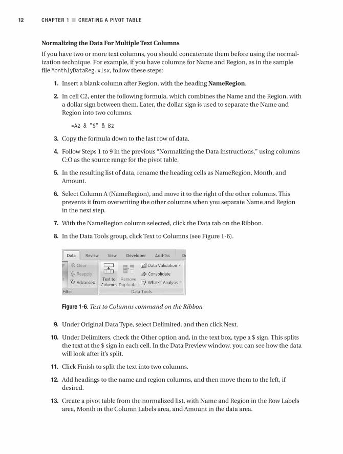
7. With the NameRegion column selected, click the Data tab on the Ribbon.

8. In the Data Tools group, click Text to Columns (see Figure 1-6).

Figure 1-6. Text to Columns command on the Ribbon

9. Under Original Data Type, select Delimited, and then click Next.

10. Under Delimiters, check the Other option and, in the text box, type a $ sign. This splitsthe text at the $ sign in each cell. In the Data Preview window, you can see how the datawill look after it’s split.

11. Click Finish to split the text into two columns.

12. Add headings to the name and region columns, and then move them to the left, ifdesired.

13. Create a pivot table from the normalized list, with Name and Region in the Row Labelsarea, Month in the Column Labels area, and Amount in the data area.


1.8. Preparing the Source Data: Using an Access Query

ProblemThe sales manager has asked you to create a pivot table from sales orders stored in a MicrosoftAccess database. You will create reports that summarize the sales orders by product and color,or by customer location, and show the total quantities and total dollars. The person who man-ages the database will create a query in the database for you to use as the data source. Thisperson has asked what fields you want to include in the query.

SolutionIn the Access query, include all the fields you want in the pivot table, and create calculatedfields if required, as the following describes.

• Include any lookup tables in the query, and add the descriptive field names to the queryoutput, instead of using ID numbers or codes. For example, suppose an OrderDetailtable includes a product number. Another table (Products) in the database contains theinformation about each product number, such as the product name and color. In thequery, add both tables, and then join the Product number field in the two tables. In thequery grid, include fields from the OrderDetail table, such as Quantity; and from theProducts table, include descriptive fields, such as Product Name and Color.

• In the Access query, create calculated fields for any line calculations you want summa-rized in the pivot table, such as LineTotal:UnitsSold*UnitPrice. Unless all productshave the same unit price, this type of calculation cannot be done in the pivot table; itmust be done in the source data.

• Do not include user-defined functions or functions specific to Microsoft Access.Although they’re permissible within Microsoft Access, user-defined functions and somebuilt-in Access functions, such as NZ, create an error (for example, “Undefined function‘NZ’ in expression”) when used outside Access. For more information on the Jet SQLexpressions used to return the data to Excel, see “Microsoft Jet SQL Reference” athttp://office.microsoft.com/en-ca/assistance/CH062526881033.aspx.

• Do not include parameters in the Microsoft Access query. In Access, you can useparameters instead of specific criteria in a query, and you are then prompted to enterthe criteria when the query runs. However, you can’t create a pivot table that’s directlybased on a parameter query or, in the pivot table, you will get the error message“[Microsoft][ODBC Microsoft Access Driver] Too few parameters. Expected 1.” Instead,create a query without parameters and, in the pivot table, you can use filters to limit thedata that’s summarized.

For more information on Access queries, see “Queries” at http://office.microsoft.com/en-us/access/CH100645771033.aspx.


1.9. Preparing the Source Data: Using a Text File

ProblemThe accounting department can provide you with a text file of the year-to-date transactions,which you can use as a data source for your pivot table. They’ve asked how you want the fileset up, and you aren’t sure what to tell them.

SolutionYou can use a delimited or fixed-width text file as the data source for a pivot table, but it’s usu-ally easier to work with a delimited file because it requires only one setting to separate thefields. If using a fixed-width file, you have to specify the start position and length of each field.

If possible, include field headings in the first row (see Figure 1-7), or you will have to addthe headings before using the file as the source for your pivot table. Also, ensure a line-breakcharacter is at the end of each record. Figure 1-7 shows the first few rows of comma-delimiteddata in the sample file ProductSales.txt.

Figure 1-7. Comma-delimited text file with headings

1.10. Preparing the Source Data: Using an OLAP Cube

ProblemYou want to base your pivot table on an OLAP cube that contains your company’s sales data,but you aren’t sure what to consider when creating the cube. You want to ensure the cube isdesigned to make the most of Excel’s pivot table features.

SolutionA whitepaper is available for download on the Microsoft web site that can guide you or theperson who is creating your OLAP cube: Excel 2007 Document: Designing SQL Server 2005Analysis Services Cubes for Excel 2007 PivotTables www.microsoft.com/downloads/details.aspx?Familyid=2D779CD5-EEB2-43E9-BDFA-641ED89EDB6C.

Although the whitepaper refers to SQL Server 2005 Analysis Services, the information willbe useful to anyone creating an OLAP cube, from any source.


1.11. Creating the Pivot Table: Using Excel Data as the Source

ProblemYou’re familiar with creating pivot tables in Excel 2003, but you can’t find the PivotTableWizard on the Ribbon in Excel 2007. You want to create a pivot table from Excel data.

SolutionBefore you create the pivot table, you should create an Excel Table from the data. This is areplacement for Excel Lists in Excel 2003, and it has many features that can make pivot tablecreation and updating easier. You can find instructions for doing this in Section 1.4. Then,follow these steps to create the pivot table.

1. Select a cell in the Excel Table and, on the Ribbon, under the Table Tools tab, click theDesign tab.

2. In the Tools group, click Summarize with PivotTable, to open the Create PivotTabledialog box.

3. Under Choose the Data That You Want to Analyze, the option Select a Table or Rangeis selected, and the name of the Excel Table should appear in the Table/Range box.

4. Select the location for your PivotTable report—either a New Worksheet, or an ExistingWorksheet—and then click OK.

5. An empty pivot table appears on the worksheet, at the location you selected. Add fieldsto the pivot table layout by checking the fields in the PivotTable Field List. The checkedfields appear in the pivot table layout on the worksheet, and in the Areas section of thePivotTable Field List.

1.12. Creating the Pivot Table: Using Excel Data on Separate Sheets

ProblemYou have an Excel Table with each region’s sales on separate sheets in your workbook, and youwant to combine all the data into one pivot table. All the sheets are set up identically, but eachcontains data for just one region. In the Create PivotTable dialog box, you can only select thedata on one worksheet, so you can’t create the pivot table from all the data.

SolutionAlthough you can create a pivot table from data on separate worksheets, the pivot table willhave limited functionality, as described in the following “Notes” section. If possible, combineall the data on one worksheet, and then create the pivot table from that source data. To createa pivot table from data on separate worksheets, you must use the PivotTable and PivotChart


Wizard, which was used to create pivot tables in Excel 2003 and earlier versions. This is not onthe Ribbon, but you can open it with a keyboard shortcut, or add it to the QAT, as described inSection 1.7.

Follow these steps to create the pivot table from data on separate worksheets, as in thesample file named MultiConsolSales.xlsx.

1. On the keyboard, press Alt+D, P, or, on the QAT, click the PivotTable and PivotChartWizard.

2. In Step 1 of the PivotTable and PivotChart Wizard, select Multiple ConsolidationRanges, and then click Next.

3. In Step 2a, select one of the page options, and then click Next. For more informationon the page options, see the following “Notes” section.

4. In Step 2b, click the Range box, select the first range, and then click Add, to add it tothe All Ranges list.

5. Repeat Step 4 for each of the remaining ranges, to add it to the list.

6. If you chose “I Will Create The Page Fields,” you can select each range, and assign fieldnames, as described in the following “Notes” section.

7. Click Next and, in Step 3, select a location for the pivot table, and then click Finish.

8. If you created page fields, you can rename them on the worksheet, where they appearin the Report Filter area. For example, select the cell that contains the label Page1, andtype Salesperson.

9. In the Column Labels drop-down list, hide any columns that contain meaninglessdata, such as Customer, which is a text field.

NotesCreating a pivot table from multiple consolidation ranges enables you to create a pivot tablefrom data in two or more separate Excel Tables. However, the result is not the same as a pivottable created from a single Excel Table. The first field is placed in the Row Labels area, theremaining field names are placed in the Column Labels area, and the values in those columnsappear in the Values area. All the Values use the same summary function, such as Sum orCount.

You can hide or show the column items, and you can use the Report Filters to filter thedata. However, there’s no setting you can change that will make a pivot table created frommultiple consolidation ranges look like a regular pivot table.


To get the best results when creating a pivot table from multiple consolidation ranges,ensure that all the ranges being used are identical in setup. Each Excel Table should have thesame column headings, in the same order, and contain the same type of data. The ranges cancontain different numbers of rows.

The first column will be used as Row Labels in the pivot table, so move the most impor-tant field to that position. In the MultiConsolSales.xlsx sample file, the Product field is in thefirst position, so the data is summarized by product.

In the PivotTable and PivotChart Wizard, after you select Multiple Consolidation Rangesas the data source, Step 2a asks, “How many page fields do you want?” You can let Excel createone page field, or you can create the page fields yourself. These appear as Report Filters in thepivot table.

Choosing Create a Single Page Field for Me

If you select this option, one page field is created automatically. In Step 2b of the PivotTableand PivotChart Wizard, you aren’t presented with any options for creating the page fields. Inthe completed pivot table, there’s one page field, and each range in the multiple consolidationranges is represented as a numbered item—for example, Item1, Item2, and Item3.

This makes it difficult to determine which data you’re viewing when you select one of theitems from the drop-down list. However, if you’re more interested in the total amounts than inthe individual ranges, this is a quick way to create the page field.

Choosing I Will Create the Page Fields

If you select this option, you can create the page fields in Step 2b of the PivotTable and Piv-otChart Wizard. To create the page fields, follow these steps:

1. In Step 2b, select each range, and add it to the All Ranges list.

2. Select the number of page fields you want to create (zero to four). In this example,there will be two page fields.

3. In the All Ranges list, select the first range.

4. You’ll use the first page field to show the salesperson names. In the drop-down list forField One, type the name of the person whose range you have highlighted in the list.

5. Each salesperson works in one of your sales regions, and you’ll use the second pagefield to show the region names. In the drop-down list for Field Two, type the regionname for the person whose range you have highlighted in the list, as shown inFigure 1-8.


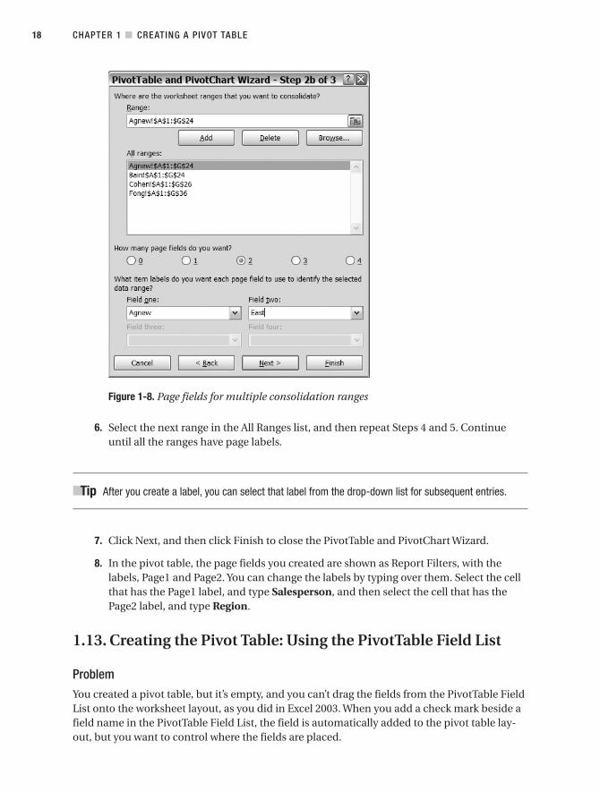
Figure 1-8. Page fields for multiple consolidation ranges

6. Select the next range in the All Ranges list, and then repeat Steps 4 and 5. Continueuntil all the ranges have page labels.

■Tip After you create a label, you can select that label from the drop-down list for subsequent entries.

7. Click Next, and then click Finish to close the PivotTable and PivotChart Wizard.

8. In the pivot table, the page fields you created are shown as Report Filters, with thelabels, Page1 and Page2. You can change the labels by typing over them. Select the cellthat has the Page1 label, and type Salesperson, and then select the cell that has thePage2 label, and type Region.

1.13. Creating the Pivot Table: Using the PivotTable Field List

ProblemYou created a pivot table, but it’s empty, and you can’t drag the fields from the PivotTable FieldList onto the worksheet layout, as you did in Excel 2003. When you add a check mark beside afield name in the PivotTable Field List, the field is automatically added to the pivot table lay-out, but you want to control where the fields are placed.


SolutionThe PivotTable Field List lists all the fields available for the pivot table, and enables you toplace the fields in specific areas of the pivot table. At the top of the PivotTable Field List is a listof the fields in your source data, in the same order they appear in the source data. At the bot-tom of the PivotTable Field List is the Areas section, with a box for each area of the pivot tablelayout; the Row Labels, the Column Labels, the Values, and the Report Filters.

When you add a check mark beside a field name in the PivotTable Field List, the field isautomatically added to a default area of the pivot table layout, but you can move the fields to adifferent area if you choose. For example, to move a field from the Row Labels area to the Col-umn Labels area, follow these steps.

1. In the PivotTable Field List, point to a field in Row Labels area.

2. When the pointer changes to a four-headed arrow, drag the field to the Column Labelsarea.

■Tip If you prefer to drag the fields onto the worksheet layout, as you did in earlier versions of Excel, youcan change a pivot table option. Right-click a cell in the pivot table, and in the context menu, click PivotTableOptions. In the PivotTable Options dialog box, click the Display tab, and add a check mark to Classic Pivot-Table Layout.

Another way to place a field in a specific area is to right-click the field name in the Pivot-Table Field List, and then select an area from the context menu (see Figure 1-9).

Figure 1-9. PivotTable Field List context menu

■Tip To remove a field from the pivot table layout, you can remove the check mark from its name in theField List section, or drag it out of the Areas section in the PivotTable Field List.


How It WorksIf you add a check mark to a numeric field in the PivotTable Field List, it is added to the Valuesarea. If you add a check mark to a nonnumeric field, it is added to the Row Labels area. Whenchecked, OLAP date and time hierarchies are automatically added to the Column Labels area.

You can add multiple copies of a field to the pivot table layout. One copy can be in theRow Labels, Column Labels, or Report Filters area, and one or more copies can be placed inthe Values area. For example, you can add the Region field to the Row Labels area, and anothercopy of the Region field to the Values area, where it would become Count of Region.

If a field is already in a Row Labels, Column Labels, or Report Filters area, and you addthat field to the area it’s currently in, it will change to the new location. If you add that field toa different one of those areas, it moves to the different area. For example, if the Region field isthe first of three fields in the Row Labels area, and you add it to the Row Labels area again, itwill move to the third position in the Row Labels area. If you add the Region field to the Col-umn Labels area, it will move from the Row Labels area to the Column Labels area.

For OLAP fields, you can only move hierarchies, attributes, and named sets to the RowLabels, Column Labels, and Report Filters areas. Measures, calculated measures, and KeyPerformance Indicators (KPIs) can only be moved to the Values area.

1.14. Creating the Pivot Table: Changing the Field List Order

ProblemMany fields are in the source data for your pivot table, and the PivotTable Field List shows thefields in the same order they appear in the source data. To make it easier to locate the fields inthe long list, you would like the field list in alphabetical order.

SolutionYou can change a pivot table option, to make the PivotTable Field List show the fields in alpha-betical order.

1. Right-click a cell in the pivot table, and in the context menu, click PivotTable Options.

2. In the PivotTable Options dialog box, click the Display tab.

3. In the Field List section, select Sort A to Z, and then click OK (see Figure 1-10).

Figure 1-10. Field List sort order

■Tip To return the field list to its original order, select Sort in Data Source Order in the PivotTable OptionsDisplay tab.


Sorting and Filtering Pivot Table Data

As you analyze data in a pivot table, you may want to rearrange the items in the Row Labelsand Column Labels areas, or sort the summarized values, to focus on products that are sellingthe best, or districts that are doing poorly. Sorting the labels or the values lets you move themost important information to the top. You can also filter the labels or the values to limit thedata summarized in the pivot table.

Unless otherwise noted, the problems in this chapter are based on data in the sample filenamed FoodSales.xlsx.

2.1. Sorting a Pivot Field: Sorting Row Labels

ProblemThree fields are in the Row Labels area of your pivot table: District, City, and Category, asshown in Figure 2-1. District, the first row field, is sorted alphabetically, and you want to sortthe districts in ascending order by their total sales. The TotalSale field is in the Values area.

Sorting the row labels alphabetically or by values is simple when only one field is in theRow Labels area, but you sometimes have problems when multiple fields exist. This problemis based on the sample file FoodSales.xlsx.

■Note If a pivot table has more than one field in the Row Labels area, the field that’s last in the list is theinner field. All the remaining row fields are outer fields. In Figure 2-1, District and City are the outer rowfields, and Category is the inner row field.

21

C H A P T E R 2

Figure 2-1. District and City are the outer row fields and Category is the inner row field.

SolutionWhen a single field is in the Row Labels area, you can select any row label or value cell, andclick the A-Z button on the Ribbon’s Data tab to sort the labels. With multiple fields, the key tosuccess lies in selecting an appropriate cell before sorting.

Sorting by Labels

To sort a field alphabetically, follow these steps:

1. Right-click a row label for the field you want to sort. For example, to sort the Districtfield’s labels, right-click the East label.

2. Click Sort, and then click Sort A to Z.

Sorting by Values

If the values or subtotals are visible, follow these steps to sort a field’s row labels by theirvalues:

1. Right-click a value cell or subtotal for the field you want to sort. For example, to sortthe District field’s values, right-click the subtotal for the Central district.

2. Click Sort, and then click Sort Largest to Smallest.

Only the row labels for the selected field will be sorted. For example, if you sort the districtlabels by their values, the city and category labels are unaffected. Also, the values are sortedwithin their group. For example, if you sort the categories by value, the categories listed undereach city are sorted by value. As a result, the categories may appear in a different order undereach city.

Sorting by Values with Hidden Subtotals

For an outer field in the Row Labels area, subtotals may be hidden. If the subtotals are not visi-ble, additional steps are required to sort the row labels by their values. Follow these steps tosort a field’s row labels by their values, in ascending order:

CHAPTER 2 ■ SORTING AND FILTERING PIVOT TABLE DATA22

1. Right-click a row label for the field you want to sort. For example, to sort the City field’slabels, right-click Boston.

2. Click Sort, and then click More Sort Options.

3. Under Sort Options, select Ascending (A to Z) by.

4. From the drop-down list, select the value field by which you want to sort. In this exam-ple, Sum of TotalSale would be the value field selected.

5. Click OK to close the Sort dialog box.

How It WorksIn a pivot table, when you do an ascending sort, values are sorted in the following order:

1. Numbers (including dates, which Excel stores as numbers).

2. Text, in the following order: 0 1 2 3 4 5 6 7 8 9 (space) ! “ # $ % & ( ) * , . / : ; ? @ [ \ ] ^ _ ` { |} ~ + < = > A B C D E F G H I J K L M N O P Q R S T U V W X Y Z.

Hyphens and apostrophes are ignored, except where two items are the same except fora hyphen. In that case, in an ascending sort, the item with the hyphen is sorted afterthe similar items without the hyphen. For example, Arrowroot would be listed before-Arrowroot.

3. Logical values (FALSE comes before TRUE).

4. Error values, such as #N/A and #NAME?. Unlike a worksheet sort, where error valuesare treated equally, error values in a pivot table are sorted alphabetically.

5. Blank cells.

2.2. Sorting a Pivot Field: New Items Out of Order

ProblemYour company has just started to sell binders, in addition to its existing products, and thismorning you entered the first order for binders in your pivot table source data. The Productfield is in the Row Labels area of the pivot table, and Quantity is in the Values area.

When you refreshed the pivot table, Binders appeared at the bottom of the Product list,instead of the top. It’s also at the bottom of the drop-down filter list for the row labels. Thismakes finding the new product in the list difficult, and you’d like it sorted alphabetically withthe other products. This problem is based on the sample file NewProduct.xlsx.

SolutionIf a field’s sort setting is set for Manual sort, new items will appear at the end of the drop-downlist. This sort setting can occur if you manually rearrange the items in the Row Labels area.Follow these steps to sort the field in ascending order:

CHAPTER 2 ■ SORTING AND FILTERING PIVOT TABLE DATA 23

1. Right-click a cell in the Product field. For example, right-click the Envelopes cell.

2. Click Sort, and then click Sort A to Z.

When you sort the field, its sort setting changes from Manual to Sort Ascending or SortDescending. This also sorts the drop-down list, and makes it easier for users to find the itemsthey need.

2.3. Sorting a Pivot Field: Sorting Items Left to Right

ProblemIn your pivot table, the City field is in the Column Labels area, the Product field is in the RowLabels area, and TotalSale is in the Values area. The city names in the column headings aresorted alphabetically.

You’re planning a new marketing campaign for bran bars, and you want to focus on thecities with the highest sales for this product. You’d like to sort the values in the Bran row fromleft to right, so the city with the highest sales for bran bars is at the left. This problem is basedon the sample file FoodSales.xlsx.

SolutionYou can sort a row label by its values, left to right. In this example, the Bran product will besorted by its TotalSale amounts. The column heading for the city with largest amount sold willbe at the left.

1. In the pivot table, right-click a value cell in the Bran row.

2. Click Sort, and then click More Sort Options, to open the Sort By Value dialog box.

3. Under Sort Options, select Largest to Smallest.

4. Under Sort direction, select Left to Right. In the Summary section, you can see adescription of the sort settings (see Figure 2-2).

5. Click OK to close the dialog box.

The TotalSale values for the Bran product are sorted largest to smallest, from left to right. TheCity column order has changed, and New York, which has the highest Bran sales, is at the left.Rows for other products may not be in descending order, because the column order has beenset by the Bran product.


Figure 2-2. Sort By Value dialog box

2.4. Sorting a Pivot Field: Sorting Items in a Custom Order

ProblemIn your pivot table, the City field is in the Row Labels area, and you would like the cities listedgeographically instead of alphabetically. You can manually rearrange the city labels, but youwould prefer to have them sorted automatically. This problem is based on the sample fileFoodSales.xlsx.

SolutionIn Excel, you can create custom lists, like the built-in lists of weekdays and months. For exam-ple, you could create a custom list of districts, department names, or reporting categories, andthen use the custom lists to sort the items in your pivot table. This enables you to createreports that are tailored to your needs, quickly and easily.

Creating a Custom List

The entries for the custom list can be imported from a worksheet list, or typed in the CustomLists dialog box. In this example, the list of cities is typed.

1. Click the Microsoft Office button, and at the bottom right, click Excel Options.

2. In the list of categories, click Popular, and in the Top Options for Working with Excelsection, click Edit Custom Lists.

3. In the Custom Lists dialog box, under Custom Lists, select NEW LIST.


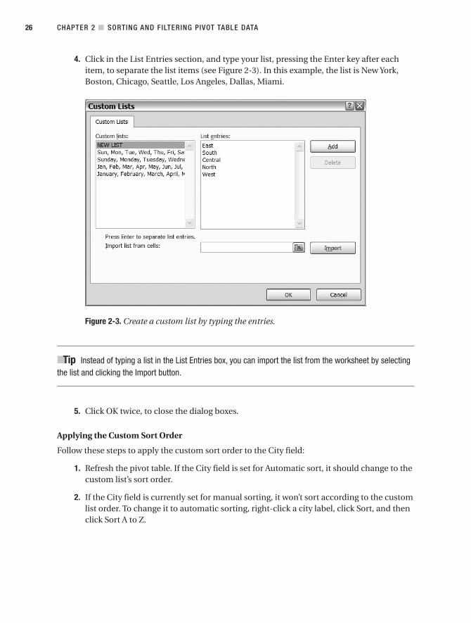
4. Click in the List Entries section, and type your list, pressing the Enter key after eachitem, to separate the list items (see Figure 2-3). In this example, the list is New York,Boston, Chicago, Seattle, Los Angeles, Dallas, Miami.

Figure 2-3. Create a custom list by typing the entries.

■Tip Instead of typing a list in the List Entries box, you can import the list from the worksheet by selectingthe list and clicking the Import button.

5. Click OK twice, to close the dialog boxes.

Applying the Custom Sort Order

Follow these steps to apply the custom sort order to the City field:

1. Refresh the pivot table. If the City field is set for Automatic sort, it should change to thecustom list’s sort order.

2. If the City field is currently set for manual sorting, it won’t sort according to the customlist order. To change it to automatic sorting, right-click a city label, click Sort, and thenclick Sort A to Z.


2.5. Sorting a Pivot Field: Items Won’t Sort Correctly

ProblemOne of your salespeople is named Jan, and her name always appears at the top of the SalesRepitems, ahead of the names that precede it alphabetically. You can manually drag her name tothe correct position in the row labels, but you’d like to know why her name is out of order, andhow you can fix the problem. This problem is based on the sample file SalesNames.xlsx.

SolutionJan goes to the top of the list because Excel assumes Jan means January, and is an item in oneof Excel’s built-in custom lists. Other names, such as May or June, would also go to the top ofthe list, because they’re also in the custom list for months. Other words may not sort asexpected if you have created other custom lists on your computer, as described in Section 2.4.For example, you may have created custom lists of districts or departments, and those liststake precedence when sorting labels in a pivot table.

If you don’t want to use custom lists when sorting in a pivot table, you can change a pivottable setting, to block their use.

■Note Changing the Use Custom Lists When Sorting setting affects all fields in the active pivot table, notjust a specific field.

1. Right-click a cell in the pivot table, and click PivotTable Options.

2. In the PivotTable Options dialog box, click the Totals & Filters tab.

3. In the Sorting section, remove the check mark from Use Custom Lists When Sorting(see Figure 2-4), and then click OK.

Figure 2-4. Use Custom Lists When Sorting.


Any custom sort orders in the pivot table are removed, and for fields that are set to auto-matic sorting, the labels are sorted in alphabetical or numerical order. To change a field toautomatic sorting, right-click a label for the field, click Sort, and then click Sort A to Z.

2.6. Filtering a Pivot Field: Filtering Row Label Text

ProblemYou’re reviewing the sales of your company’s mid-priced products and, in your pivot table,UnitCost and Product are in the Row Labels area, District is in the Column Labels area andTotalSale is in the Values area. You’d like to view only the data for the products with a unit costbetween $0.40 and $0.70, but you don’t want to uncheck all the other items in the UnitCostfield’s filter list. This problem is based on the sample file FoodSales.xlsx.

SolutionTo limit what’s displayed in the pivot table, you can filter the row labels. In this example, youfilter to show only the unit costs within a specific range. To apply the filter, follow these steps:

1. Click the drop-down arrow in the Row Labels heading, and in the Select Field drop-down list, select UnitCost.

■Tip If you select a UnitCost row label before clicking the arrow, that field name will be the default selec-tion in the drop-down list.

2. Click Label Filters, and then click Between.

3. In the Label Filter dialog box, leave the drop-down box with the selection Is Between.In the text box where the cursor is flashing, type .4, which is the minimum unit costyou want included.

4. In the second text box, type .7, which is the maximum unit cost you want included,and then click OK.

The filter is applied to the labels, and UnitCost labels between $0.40 and $0.70 are visible.A filter icon appears in the Row Labels drop-down arrow. Another filter icon appears to theright of the UnitCost field in the PivotTable Field List.

■Note The minimum and maximum values are included when the Between filter is used, so values of$0.40 and $0.70 are shown in the filtered results for this example.


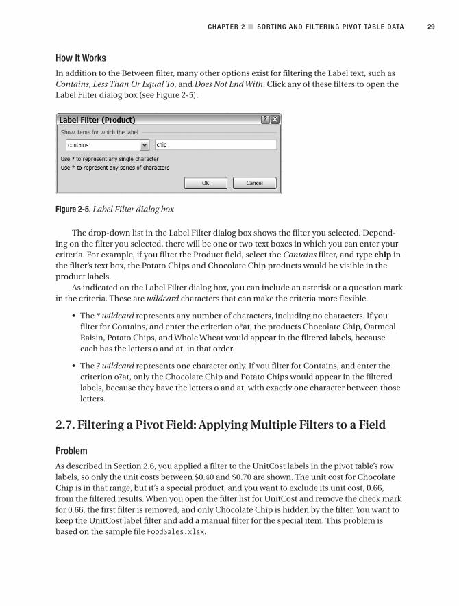
How It WorksIn addition to the Between filter, many other options exist for filtering the Label text, such asContains, Less Than Or Equal To, and Does Not End With. Click any of these filters to open theLabel Filter dialog box (see Figure 2-5).

Figure 2-5. Label Filter dialog box

The drop-down list in the Label Filter dialog box shows the filter you selected. Depend-ing on the filter you selected, there will be one or two text boxes in which you can enter yourcriteria. For example, if you filter the Product field, select the Contains filter, and type chip inthe filter’s text box, the Potato Chips and Chocolate Chip products would be visible in theproduct labels.

As indicated on the Label Filter dialog box, you can include an asterisk or a question markin the criteria. These are wildcard characters that can make the criteria more flexible.

• The * wildcard represents any number of characters, including no characters. If youfilter for Contains, and enter the criterion o*at, the products Chocolate Chip, OatmealRaisin, Potato Chips, and Whole Wheat would appear in the filtered labels, becauseeach has the letters o and at, in that order.

• The ? wildcard represents one character only. If you filter for Contains, and enter thecriterion o?at, only the Chocolate Chip and Potato Chips would appear in the filteredlabels, because they have the letters o and at, with exactly one character between thoseletters.

2.7. Filtering a Pivot Field: Applying Multiple Filters to a Field

ProblemAs described in Section 2.6, you applied a filter to the UnitCost labels in the pivot table’s rowlabels, so only the unit costs between $0.40 and $0.70 are shown. The unit cost for ChocolateChip is in that range, but it’s a special product, and you want to exclude its unit cost, 0.66,from the filtered results. When you open the filter list for UnitCost and remove the check markfor 0.66, the first filter is removed, and only Chocolate Chip is hidden by the filter. You want tokeep the UnitCost label filter and add a manual filter for the special item. This problem isbased on the sample file FoodSales.xlsx.


SolutionWhen a pivot table is created, its default setting is to allow only one filter at a time on eachfield. You applied a label filter to the UnitCost field, and it was automatically removed whenyou applied a manual filter on the same field. To allow more than one filter, you can change asetting in the pivot table options:

1. Right-click a cell in the pivot table, and then click PivotTable Options.

2. On the Totals & Filters tab, add a check mark to Allow Multiple Filters Per Field (seeFigure 2-6), and then click OK.

Figure 2-6. Allow multiple filters per field.

You can now click the drop-down arrow on the Row Labels heading and remove the checkmark from the special product’s unit cost. The label filter will be retained, and the manual fil-ter will be added.

How It WorksThree types of filters can be applied to the row labels and column labels: label (or date) filters,value filters, and manual filters. If the Allow Multiple Filters Per Field setting is turned off, onlyone type of filter can be applied to a field. As soon as you apply a different type of filter, thefirst filter is automatically removed, without warning.

■Note Only one of each type of filter can be applied to a field. For example, even if the Allow MultipleFilters Per Field setting is turned on, you can only apply one label filter to the Product field.

If the Allow Multiple Filters Per Field setting is turned on, one of each type of filter can beapplied to a field. You can filter the labels for a date range, or for specific text. Then, you canapply a manual filter, to exclude other items from the filtered results. Finally, you can filter thefield based on its values, to show only the items with a row or column total over a specificamount, or in a set range.

To see the filters and sort options that were applied in the pivot table, you can point to thedrop-down button on the Row Labels or Column Labels heading cell. In the pivot table shownin Figure 2-7, the UnitCost field has three filters applied, the City field has two filters applied,and the District field is sorted in ascending order.


Figure 2-7. Viewing the filter and sort details

2.8. Filtering a Pivot Field: Filtering Row Label Dates

ProblemIn your pivot table, you have sales results for all your sales districts, with District and Sales-Week fields in the Row Labels area and TotalSale in the Values area. At the beginning of eachmonth, you have to prepare a report to summarize the data from the previous month. You’dlike to find a quick way to select the SalesWeek items you need, so it’s easier to create thereport. This problem is based on the sample file FoodSales.xlsx.

SolutionWhen a date field is in the Row Labels or Column Labels area, you can filter the labels to showonly the dates in a specific range, such as next week, or last month. To apply the filter, followthese steps:

1. Click the drop-down arrow in the Row Labels heading.

2. In the Select Field drop-down list, select the SalesWeek field.

3. Click Date Filters, and then click Last Month.

The filter is applied to the labels, and the pivot table now shows a summary of sales in theprevious month. A filter icon appears in the Row Labels drop-down arrow, and another filtericon appears to the right of the SalesWeek field in the PivotTable Field List.

■Tip In the PivotTable Options dialog box, on the Data tab, add a check mark to Refresh Data When Open-ing the File, to ensure the dynamic date range is up-to-date.


How It WorksThere are two types of date filters—specific date range, and dynamic date range. When the fil-ter criteria can change automatically, such as Last Week, or Next Month, it is called a dynamicfilter. For other date filters, you use a comparison operator, such as Equals, or Between, andrefer to a specific date or dates in the criteria (see Figure 2-8). When a comparison operator(Equals, Greater Than, Less Than, or Between) is used in a filter, it is called a common filter.

Figure 2-8. Filter for a specific date range

2.9. Filtering a Pivot Field: Filtering Values for Row Fields

ProblemIn your pivot table, you have sales results for all your districts, with District in the ColumnLabels area, SalesWeek in the Row Labels area, and TotalSale in the Values area. You haveremoved all the filters from the pivot table, and now you’d like to view all the weeks in whichthe total sales are between $2000 and $5000. This problem is based on the sample file Food-Sales.xlsx.

SolutionYou can filter the row grand total values, to show only the rows that meet the criteria.

■Note The Grand Total for rows does not have to be visible to use the Row Labels Value filters.

1. In the pivot table, click the arrow on the Row Labels heading.

2. Click Value Filters, and then click Between.


3. In the third box, enter 2000 as the minimum dollar amount and, in the fourth box,enter 5000 as the maximum dollar amount. The values entered in the minimum andmaximum boxes will be included in the filter results. In this example, any weeks withtotal sales from 2000, up to and including 5000, will be shown.

■Note The values must be typed into the Value Filter dialog box. You can’t use a cell reference to providethe criteria for a value filter.

4. Click OK, to apply the filter.

Only the weeks with total sales between the minimum value and maximum value (inclusive)remain visible.

NotesThe Row Labels Value filters can only be applied on the grand total for the row. Other values inthe row cannot be filtered. For example, in the pivot table shown in Figure 2-9, you can’t filterfor SalesWeeks with a value greater than $1000 in the South District. You can only filter forSalesWeeks where the grand total value meets your criteria.

Figure 2-9. Filter for grand total values only

If you want to filter for values in a specific district, you can hide all the other districts, sothe grand total reflects only the values for the visible district. Then, apply a filter, and it willshow the results for the visible district.

2.10. Filtering a Pivot Field: Filtering for Nonconsecutive Dates

ProblemIn your pivot table, the WorkDate field is in the Row Labels area and LbrHrs is in the Valuesarea. You want to see the data from three nonconsecutive dates, when the service departmentwas short-staffed. When you use the row label date filters, you can only select a consecutivedate range, or one specific date. You can’t select the three dates you need. This problem isbased on the sample file Service.xlsx.


SolutionInstead of using the date filter options, you can manually select or deselect the items in theRow Labels drop-down list. You can use this manual filter option if you want to select specificitems that can’t be filtered by using a common or dynamic filter. To manually filter dates in theRow Labels filter list, follow these steps:

1. In the pivot table, click the arrow on the Row Labels heading.

2. In the list of dates, remove the check mark from Select All, to remove all the checkmarks from the list.

3. Add check marks to the dates you want to see, and then click OK.

The pivot table now shows results for work done on the selected dates, and you can focus onthat data.

■Note A manual filter is retained if a filtered field is moved to the Report Filter area, but a label or valuefilter is removed.

2.11. Filtering a Pivot Field: Including New Items in a Manual Filter

ProblemIn your pivot table, WorkDate is in the Row Labels area and LbrHrs is in the Values area. Youmanually applied a filter to the WorkDate field in the Row Labels area of your pivot table.When you updated the pivot table, some new dates appeared in the pivot table, even thoughthey were not the dates selected in the manual filter. This problem is based on the sample fileService.xlsx.

SolutionYou can change a setting in the WorkDate field, to specify if new items are included or not,when the field is manually filtered. To change the setting, and prevent new items from beingincluded, follow these steps:

1. In the pivot table, right-click a cell in the WorkDate Row Labels, and click Field Set-tings.

2. On the Subtotals & Filters tab, in the Filter section, remove the check mark fromInclude New Items in Manual Filter, and then click OK (see Figure 2-10).


Figure 2-10. Clear the Include New Items in Manual Filter check box.

■Tip You can turn this setting on if you want to ensure that you notice new records when they’re added,and you can manually deselect them after they appear.

2.12. Filtering a Pivot Field: Filtering by Selection

ProblemIn your pivot table, the Product field is in the Row Labels area and UnitsSold is in the Valuesarea. Frequently, you want to view a summary for two or three of the products, and you’d like aquick way to hide the other products. This problem is based on the sample fileFoodSales.xlsx.

SolutionTo quickly filter the labels in a pivot table, you can select one or more labels, and then use theselection to filter the pivot table. To filter for three of the Product labels, follow these steps:

1. Click a cell that contains one of the Product row labels you want to filter, to select thatlabel.

2. Hold the Ctrl key on the keyboard, and click two other Product row labels, to selectthem.

3. Right-click one of the selected labels.

4. In the context menu, click Filter, and then click Keep Only Selected Items.

■Note At least one row label must remain visible.

Only the three selected products are visible, and all the other data is hidden. This is like man-ual filtering; if you look at the list of dates in the Row Labels drop-down, the three selecteddates have check marks, and all the other dates have their check marks cleared.


Sometimes, you may want to hide a few selected items, and leave all the other items visi-ble. Follow these steps to hide some items:

1. Select one label cell, or select a single block of label cells.

2. Right-click one of the selected cells.

3. In the context menu, click Filter, and then click Hide Selected Items.

This leaves all the labels visible, except the selected items.

2.13. Filtering a Pivot Field: Filtering for Top Items

ProblemIn your pivot table, the Product field is in the Row Labels area, the District field is in the Col-umn Labels area, and the UnitsSold field is in the Values area. The sales manager is preparinga forecast for next year, and he has asked you for a report that shows only the three productswith the highest number of units sold. This problem is based on the sample fileFoodSales.xlsx.

SolutionYou can use the Top 10 Filter for the Product row labels, to filter the values. Follow these stepsto apply the filter.

1. Right-click a cell that contains a Product row label, and in the context menu, clickFilter, and then click Top 10.

2. In the Top 10 Filter dialog box, select Top from the first drop-down list, and in the sec-ond box, enter a 3.

3. From the third box, select Items, and in the last box, select Sum of UnitsSold, and thenclick OK.

The pivot table shows only the three products with the highest number of units sold, basedon the grand total for each row.

■Note If a tie occurs in the number of units sold, more than three products may be shown.

How It WorksAlthough the filter feature is called Top 10, you can use it to filter for the highest or lowest val-ues, and you can choose a number other than 10. In the first drop-down list in the Top 10Filter dialog box, you can choose Top or Bottom, to see either the highest or lowest values. Inthe second box, you can type any number, to limit the records that will be visible in the filteredpivot table. In the third drop-down list, you can select Items, Percent, or Sum. In the fourthdrop-down list, you can choose one of the Value fields in the pivot table.


Filtering for Items

If you select Items in the third drop-down list, a specific number of items, with the highest orlowest grand total amounts, is displayed when you apply the filter. This number may beexceeded if ties are in the grand totals. For example, if you filter for the Top 2 Items, and threegrand totals are tied for second highest, all three, plus the highest value, would be filtered.

Filtering for Percent

If you select Percent in the third drop-down list, items with the highest or lowest grand totalamounts, that comprise the specified percent of the overall grand total, will be displayed whenyou apply the filter.

In the FoodSales.xlsx example, the pivot table has a grand total of 256,941 units sold.If you select to show the Bottom 20 Percent, you can see the products with the lowest grandtotals for units sold, that combine to total at least 20 percent of that overall grand total, orapproximately 51,000 units sold. The bottom six products have a total of only 42,517 units,which is less than 20 percent, so the bottom seven products are returned in the filter.

You could use this feature to determine where to focus your improvement efforts. Onlya few clients or products may contribute to the top 10 or 20 percent of your sales, and severalhundred comprise the remaining percent of sales. Using a top or bottom filter can help youidentify those clients or products.

Filtering for Sum

If you select Sum in the third drop-down list, items with the highest or lowest grand totalamounts, that total at least the specified sum, are displayed when you apply the filter.

In the FoodSales.xlsx example, if you selected to show the Top 100,000 Sum, when youapply the filter, you can see the products with the highest grand totals for units sold, that com-bine to total at least 100,000 units sold. Only two products, Potato Chips and Saltines, arereturned in the filter, because these two have combined sales of 123,458.

2.14. Using Report Filters: Hiding Report Filter Items

ProblemThe Product field is in the Report Filter area of your pivot table, and (All) has been selectedfrom its drop-down list. The sales manager would like you to exclude the Cheese and Branproducts from the report, and summarize all the other products. You don’t see any way to hidesome of the products in the Report Filter. Unlike the row and column labels, the Report Filter’sdrop-down list doesn’t have check boxes to indicate which items to show and which to hide.This problem is based on the sample file FoodSales.xlsx.

SolutionYou can change a setting in the Report Filter so it enables you to select items to show or hide.Follow these steps to change the setting:


1. Click the drop-down arrow for the Product Report Filter, and at the bottom of the itemlist, add a check mark to Select Multiple Items.

2. Remove check marks for the items you want to hide, and then click the OK button toclose the list. At least one item must be selected, or the OK button won’t be enabled.

The Report Filter will show (Multiple Items) instead of (All), if the Select Multiple Itemsoption is turned on, and not all items are selected.

2.15. Using Report Filters: Filtering for a Date Range

ProblemThe sales manager has asked for a report on the total sales for October. The SalesWeek field isin the Report Filter area of your pivot table, but you don’t want to manually hide all the datesthat aren’t in October. The Filter Date feature isn’t available when the SalesWeek field is in theReport Filter area. This problem is based on the sample file FoodSales.xlsx.

WorkaroundIf this is a one-time requirement, it might be quickest to remove the check mark from the (All)item in the Report Filter, and then check the October dates.

If you’ll need frequent reports for a month’s data, you could group the SalesWeek field,and then filter for a specific month, instead of individual dates. Follow these steps to groupthe dates:

1. Temporarily move the SalesWeek field to the Row Labels area. You can’t group the dateswhile the field is in the Report Filter area.

2. Right-click one of the cells that contains a SalesWeek label, and then click Group.

3. In the Grouping dialog box, the earliest and latest dates in the SalesWeek field shouldautomatically appear in the Starting at and Ending at date boxes.

4. In the By list, click Months, to select it. If other options are highlighted, click them, todeselect them. This groups all the data for each month, across multiple years. If youneed to report on the years separately, also select Years in the By list.

5. Click OK to close the Grouping dialog box.

6. Move the SalesWeek field back to the Report Filter area, and then filter for October.

2.16. Using Report Filters: Filtering for Future Dates

ProblemThe warehouse manager has asked you for a report that shows the product quantities fororders with future ship dates. In your pivot table, ShipDate is in the Report Filter area, Productis in the Row Labels area, and Units is in the Values area.


The date filters aren’t available in the Report Filter, and you don’t want to manually hideall the past dates in the ShipDate Report Filter. This problem is based on the sample fileShipped.xlsx.

WorkaroundFor some filtering problems, the best solution is to add a column to the source data. In thenew column, you can enter a formula or a value, and use that data in the pivot table. In thiscase, a column can be added, with a formula to test if the ship date is later than the currentdate.

1. In the source data table, add a column with the heading ShipLater.

2. In the first data row of the new column, enter a formula that refers to the ShipDate inthat row—for example, =A2 > TODAY().

3. Copy the formula down to the last row of data. If the source data has been formattedas an Excel Table, the formula should automatically copy down to the last row in thetable.

4. Refresh the pivot table, and add the ShipLater field to the Report Filter area.

5. From the ShipLater Report Filter drop-down list, select TRUE.

■Note Refresh the pivot table each day to see the current calculations for the ShipLater field. In the PivotTable Options dialog box, on the Data tab, you can add a check mark to Refresh Data When Openingthe File.


Calculations in a Pivot Table

In a pivot table, you can use functions like Sum, Count, or Average to summarize the fieldsyou place in the Values area. You can also use custom calculations, such as Difference From,and Running Total, to show a different perspective on the data. For even greater flexibility, youcan write your own formulas to create calculated fields and calculated items in the pivot table.

3.1. Using Summary Functions: Defaulting to Sum or Count

ProblemThe sales manager sent you a workbook with sales data, and she asked you to create a pivottable from the data. You added the Product field to the Row Labels area, the District field to theReport Filter area, and Units and TotalSales to the Values area.

When you added the Units field to the Values area, it automatically used the Sum func-tion, but when you added the TotalSales field to the Values area, it used the Count function.You’re not sure why different functions were used for two fields that both contain numbers.This problem is based on the OfficeSales.xlsx sample file.

SolutionPerhaps blank cells were in the source data for the TotalSales field. If you add a number field tothe Values area, the default summary function is Sum. However, if blank cells, or nonnumericdata, such as text or errors, are in the field, the Count function is used as a default.

■Note You cannot change the default summary function in a pivot table. Either Sum or Count will be used,depending on the field’s contents.

After a field has been added to the Values area, you can change its summary function,unless the field is a calculated field, or the pivot table is based on an OLAP data source:

1. Right-click a cell in the field you want to change, and click Summarize Data By.

2. Click one of the functions in the menu (see Figure 3-1).

41

C H A P T E R 3

Figure 3-1. Select a summary function.

3. If the function you want is not visible, click More Options. Click a function in the Sum-marize Value Field By list, and then click OK (see Figure 3-2).

Figure 3-2. The Value Field Settings dialog box with a list of summary functions

■Tip You can add two copies of a field to the pivot table’s Values area, and use a different summary func-tion for each copy. For example, show the Sum of Units and the Average of Units.

How It WorksWhen you add a field to the pivot table’s Values area, a list of 11 functions (listed as follows) isavailable to summarize the data. Only these functions are available when summarizing thepivot table data; other functions, such as Median, Mode, and Percentile, can be calculatedfrom the source data, outside the pivot table.

The summary functions in a pivot table are similar to the worksheet functions with thesame names, with a few differences as noted in the descriptions that follow.

Sum

Sum is the default summary function for numerical fields added to the pivot table’s Valuesarea, and it totals all the underlying values in the Values area. The result is the same as usingthe SUM function on the worksheet to total the values.

CHAPTER 3 ■ CALCULATIONS IN A P IVOT TABLE42

Count

Count is the default summary function when fields with nonnumeric or blank cells are addedto the Values area. Like the COUNTA worksheet function, the pivot table Count function countstext, numbers, and errors. Blank cells are not counted.

Average

The Average function totals all the underlying values in the Values area, and it divides by thenumber of values. The result is the same as using the AVERAGE function on the worksheet tocalculate the average (mean) of the values.

Max

The Max summary function shows the maximum value from the underlying values in theValues area. The result is the same as using the MAX function on the worksheet to calculatethe maximum of the values.

Min

The Min summary function shows the minimum value from the underlying values in theValues area. The result is the same as using the MIN function on the worksheet to calculatethe minimum of the values.

Product

The Product summary function shows the result of multiplying all the underlying values inthe Values area. The result is the same as using the PRODUCT function on the worksheet tocalculate the product of the values. The results of this function may be very large numbersand default to a Scientific number format. Excel only stores and calculates with 15 significantdigits of precision, so after the 15th character you’ll only see zeros.

Count Numbers

The Count Numbers summary function counts all the underlying numbers in the Values area.The result is the same as using the COUNT function on the worksheet. Blank cells, errors, andtext are not counted.

StDev

Like the STDEV worksheet function, the StDev summary function calculates the standarddeviation for the underlying data in the Values area.

If the count of items is one, a #DIV/0! error is displayed, because one is subtracted fromthe count when calculating the standard deviation.

There may be differences between the worksheet results and the pivot table results,because the worksheet function was improved in Excel 2003, but the pivot table function wasnot changed. For more information, see the Microsoft Knowledge Base article “Description ofImprovements in the Statistical Functions in Excel 2003 and in Excel 2004 for Mac,” at http://support.microsoft.com/default.aspx?kbid=828888.

CHAPTER 3 ■ CALCULATIONS IN A P IVOT TABLE 43

StDevp

Like the STDEVP worksheet function, the StDevp summary function calculates the standarddeviation for the entire population for the underlying data in the Values area. In Excel 2003,improvements were made to several statistical functions, including STDEV and STDEVP. Seethe previous “StDev” section for more information.

Var

Like the VAR worksheet function, the Var summary function calculates the variance for theunderlying data in the Values area, and is the square of the standard deviation.

If the count of items is one, a #DIV/0! error is displayed, because one is subtracted fromthe count when calculating the standard deviation.

In Excel 2003, improvements were made to several statistical functions, including VARand VARP. The Var and Varp summary functions have been improved when used in the interiorof the PivotTable report, but not for grand totals for rows or columns. For more information,see the Microsoft Knowledge Base article “Excel Statistical Functions: VAR and VARP Improve-ments and Pivot Tables,” at http://support.microsoft.com/default.aspx?kbid=829250.

Varp

The Varp summary function calculates the variance for the entire population for the under-lying data in the Values area. In Excel 2003, improvements were made to several statisticalfunctions, including VAR and VARP. See the previous “Var” section for more information.

Errors in the Source Data

The Count and Count Numbers functions handle errors as outlined earlier. For other sum-mary functions, if errors are in the source data field, the first error encountered is displayed inthe pivot table, and the total is not calculated. If subtotals, or row and column totals, are dis-played, affected totals and subtotals display the error.

For example, the source data shown in Figure 3-3, from the sample fileOfficeSalesError.xlsx, has two errors for West Binder data—a #REF! error and an #N/A error.

Figure 3-3. Errors in the sample source data

The first error, #REF!, appears in the pivot table, when West Binder TotalSales are summed(see Figure 3-4). If the dates in the source Excel table were sorted in descending order, the#N/A error would be listed first, and would appear in the pivot table.


Figure 3-4. The first error in the source Excel table appears in the pivot table.

3.2. Using Summary Functions: Counting Blank Cells

ProblemThe sales manager sent you a workbook with sales data, and blank cells are in the District col-umn for some records. You want to show a count of the blank District cells in the pivot table,so you can let the sales manager know how many records are incomplete.

You added the District field to the pivot table’s Row Labels area, and another copy of theDistrict field in the Values area, as Count of District. However, no count is showing for theblank districts (see Figure 3-5). This problem is based on the OfficeSales.xlsx sample file.

Figure 3-5. Blank cells are not counted in the Values area.

SolutionThe Count function doesn’t count blank cells, so when you add the District field to the Valuesarea, it has nothing to count for those blank records. Add a different field to the Values area,and use it for the count. For example, if the Units column in the source data has a value inevery row, add Count of Units to the Values area (see Figure 3-6). With District in the RowLabels area, the count of blank Districts is calculated.

Figure 3-6. Use a different field to count blank cells.


3.3. Using Custom Calculations: Difference From

ProblemEvery morning, you download the regional sales data from your sales system. You’d like to usethe pivot table to calculate each day’s change from the previous day, to obtain the daily salesfigures for each region.

In your pivot table, Date is in the Row Labels area, Region is in the Column Labels area,and Sum of Units is in the Values area, as shown in Figure 3-7. The example shown is from theRegionCalcs.xlsx workbook.

Figure 3-7. The pivot table shows units sold to date for each region.

SolutionTo supplement the summary functions, custom calculations are available when summarizingdata in a pivot table. In addition to the default normal calculation, custom calculations pro-vide eight different ways of viewing the summary results. For this problem, use the DifferenceFrom custom calculation to compare each day’s total to the previous day’s total.

■Tip Custom calculations are only available for pivot tables based on non-OLAP sources.

1. Right-click a cell in the Values area, and then click Value Field Settings.

2. On the Show Values As tab, from the drop-down list for Show Values As, select Differ-ence From.

3. You want to compare the results from one date to another, so for the base field, selectDate.

■Caution If you select a base field that isn’t in the Row or Column Labels area, all the results show an#N/A error.

4. You want to compare each date’s results to the previous date’s results, so for the Baseitem, select (previous) (see Figure 3-8), and then click OK.


Figure 3-8. Difference From settings

The values in the pivot table change, to show the difference in values, from each date tothe previous date. The row for the first date is empty, because there’s no previous date withwhich to compare it. The remaining rows show the change from the previous day in units soldfor each region (see Figure 3-9).

Figure 3-9. The custom calculation Difference From compares daily sales totals.

How It WorksThe Difference From custom calculation compares each item in the field to another item inthe same field. In this example, (previous) was selected, so each day’s total is compared to theprevious day’s total. If days are missing or hidden, the comparison is made to the previous vis-ible day.

Instead of (previous), you could select (next) to compare each day to the next visible day’stotals, or select a specific date to compare all days to the sales for the selected date.

Using the same sample data, you could select Region as the Base Field, and Central as theBase Item, to compare each region’s sales to sales in the Central Region (see Figure 3-10).

Figure 3-10. The custom calculation Difference From, with Region as a base field


3.4. Using Custom Calculations: % Of

ProblemYou have monthly sales figures for each region, and would like to compare average sales foreach region to the average sales in your strongest region.

In your pivot table, Date is in the Row Labels area, grouped by Month; Region is in theColumn Labels area; and Sum of Units is in the Values area (see Figure 3-11). The exampleshown is from the RegionWeeks.xlsx workbook.

Figure 3-11. Sum of Units per Month per Region

SolutionWhile using the custom calculations, you can use different summary functions for the data.For this problem, instead of Sum, you can use Average and the % Of custom calculation.


2. On the Summarize By tab, select Average as the type of calculation.

3. Click the Show Values As tab, and from the drop-down list for Show Values As, select % Of.

4. You want to compare the results from one region to another, so for the Base field,select Region.

5. You want to compare the results for each region to East, which has the strongest sales,so for the Base item, select East.

6. To reduce the number of decimal places, click Number Format, and format withPercentage, and the number of decimal places you want.


The pivot table values change, to show each value as a percent of the East’s sales. The columnfor the East region shows 100%, because it’s being compared to itself. The remaining columnsshow the percent of their average units per sale, compared to the East region’s average unitsper sale (see Figure 3-12).


Figure 3-12. The custom calculation % Of, with Region as a base field

3.5. Using Custom Calculations: % Difference From

ProblemYou have monthly sales figures and forecasts for each product, and you would like to compareactual sales to forecast sales for each product per month.

In your pivot table, Date (grouped by Month) and Product are in the Row Labels area, Sta-tus (Actual or Forecast) is in the Column Labels area, and Sum of Units is in the Values area(see Figure 3-13). The example shown is from the ProductSales.xlsx workbook.

Figure 3-13. Actual and Forecast values per month

SolutionUse the % Difference From custom calculation to compare the Actual to Forecast items in theStatus field. You can leave the original copy of the Sum of Units field, so you can see the Unitsquantity, as well as the % Difference From calculation.

1. Add another copy of the Units field to the Values area, where it will become Sum ofUnits2. Select a cell that contains the Sum of Units2 label, and then type a moredescriptive name, for example, % Diff.

2. Right-click one of the % Diff cells in the Values area, and click Value Field Settings.

3. Click the Show Values As tab, and from the drop-down list for Show Values As, select % Difference From.

4. You want to compare the Status field values, so for the Base field, select Status.


5. The Actual values will be compared to the Forecast values, so for the Base item, selectForecast.

6. To reduce the number of decimal places, click the Number Format button, and formatwith Percentage, and the number of decimal places you want.


8. In the PivotTable Field List, move the Status field below the ∑Values field in the Col-umn Labels area. This changes the order of the columns, so the Units are together, andthe % Diff columns are together (see Figure 3-14).

Figure 3-14. The % Difference between Actual and Forecast

The Forecast column is empty in the % Diff field, because it won’t be compared to itself.The Actual column shows the % Difference From calculation from the forecast in units sold,for each product for each month.

3.6. Using Custom Calculations: Running Total

ProblemYou have monthly sales figures for each product, and the sales manager has asked for a run-ning total of units sold by month. In your pivot table, Date (grouped by Month) is in the RowLabels area, Product is in the Column Labels area, and Sum of Units is in the Values area (seeFigure 3-15). Status is in the Report Filter area, with Actual selected. The example shown isfrom the ProductSales.xlsx workbook.

Figure 3-15. Actual product sales per month


SolutionUse a running total in a custom calculation to accumulate the sales amounts per product,down through the list of months.


2. Click the Show Values As tab, and from the drop-down list for Show Values As, selectRunning Total In.

3. You want to see the running total by month, so for the Base field, select Date, and thenclick OK. No base item is required for a running total calculation.

■Caution If you select a base field that isn’t in the Row or Column Labels area, all the results will showan #N/A error. Also, if an error exists in any month’s results, it will carry down through the remaining months.

With Date as the base field, each Product column shows a running total for the year, bymonth (see Figure 3-16). The Grand Total column shows the overall running total.

Figure 3-16. Running total by month per product

NotesIf dates in a pivot table are grouped by year and month, the running total will stop at the endof each year, and then begin again at the start of the next year. There is no setting you canadjust to change this behavior.

In the sample file ProductYear.xlsx, product sales dates range from October 2008 toMarch 2009, and they are grouped by year and month in the pivot table. Product is in theColumn Labels area, Years and Date are in the Row Labels area, and Units is in the Values area.

If you calculate a running total with Date as the base field:

• The subtotals for Years are automatically hidden when the running total is applied.

• The total for each product accumulates from October to December of 2008, and beginsagain in January 2009.


If you calculate a running total with Years as the base field:

• The subtotals for Years display the running total for each product, from one year tothe next.

• The months display the sales per month, not a running total.

To create a running total that continues from December 2008 to January 2009, you canfollow these steps to create a field in the source data, and then use it as the base for the run-ning total:

1. Add a column to the source data, with the heading YearMonth.

2. Enter a formula to return the year and month of the date in each row. For example, use this formula if the date is in Column A:

=TEXT(A2, "yyyy-mm")

3. Refresh the pivot table, add the YearMonth field to the Row Labels area, and thenremove the Date and Year fields.

4. Create a running total with YearMonth as the base field.

3.7. Using Custom Calculations: % of RowYou have monthly sales figures for each Sales Manager, and you would like to see what percentof their total sales came from each product category. In your pivot table, Sales Manager is inthe Row Labels area, Category is in the Column Labels area, and Sum of Units is in the Valuesarea (see the table at the left in Figure 3-17). The example shown is from theManagerSales.xlsx workbook.

SolutionBecause the category sales for each manager are listed across a row, you can use the % of Rowcustom calculation to show the percent per category for each Sales Manager’s sales.


2. Click the Show Values As tab, and from the drop-down list for Show Values As, select %of Row, and then click OK.

■Note There’s no option to select a base field or base item with this custom calculation.

In the row for each Sales Manager, you can see the percent of the total sold in each cate-gory (see the table at the right in Figure 3-17).

■Tip You can hide the Grand Total for Rows, because it will always equal 100 percent.


Figure 3-17. The % of Row custom calculation shows category sales percentages.

3.8. Using Custom Calculations: % of Column

ProblemYou have monthly sales figures for each product Category, and you would like to see whatpercent of their total sales were attributed to each sales manager. In your pivot table, SalesManager is in the Row Labels area, Category is in the Column Labels area, and Units is in theValues area (see the table at the left in Figure 3-18). The example shown is from theManagerSales.xlsx workbook.

SolutionBecause the sales in each category are listed down a column, you can use the % of Columncustom calculation to show the percent of sales from each Sales Manager.


2. Click the Show Values As tab, and from the drop-down list for Show Values As, select %of Column, and then click OK.

In the column for each Category, you can see the percent of the total for each sales manager(see the table at the right in Figure 3-18).

Figure 3-18. The % of Column custom calculation shows sales manager percentages.

NotesUnfortunately, there’s no % of Subtotal custom calculation option, but you can modify thepivot table layout to achieve a similar result, using % of Row or % of Column.


For example, if Category and SalesMgr are both in the Row labels area, there’s no customcalculation that shows what percent of Bar sales were by Parent. With that layout, if you usethe % of Column custom calculation, it shows the percent of the grand total for each salesmanager for each product.

Change the layout so Category is in the Columns area, as shown in the table at the right inFigure 3-18, and apply a % of Column custom calculation, to see the percent sold by eachmanager in each category.

3.9. Using Custom Calculations: % of Total

ProblemYou have monthly insurance policy counts for your regional offices. You’d like to see what per-centage of the existing policies are in each region, for auto policies and property policies. Inyour pivot table, Region is in the Row Labels area, PolicyType is in the Column Labels area,and the Sum of Policies field is in the Values area. Status is in the Report Filters area, and Exist-ing is selected (see the table at the left in Figure 3-19). The example shown is from thePolicies.xlsx workbook.

SolutionTo see the percent that each policy type per region contributes to the overall total, you can usethe % of Total custom calculation.


2. Click the Show Values As tab, and from the drop-down list for Show Values As, select % of Total, and then click OK.

In each cell, you can see the percent of the total sold in each region for each policy type (seethe table at the right in Figure 3-19). The grand total column shows the percent of total poli-cies in each region, and the grand total row shows the percent of policies in each policy type.

Figure 3-19. The % of Total custom calculation shows percentage policy type by region.


3.10. Using Custom Calculations: Index

ProblemYou have monthly insurance policy counts for your regional offices. You’d like to compare can-celed policies in each region, for both auto policies and property policies. In your pivot table,Region is in the Row Labels area, PolicyType is in the Column Labels area, and Sum of Policiesis in the Values area. Status is in the Report Filters area, and Cancel has been selected (see thetable at the left in Figure 3-20). The example shown is from the Policies.xlsx workbook.

SolutionUse the Index option to show the relative weight of each cell when compared to its row total,its column total, and the grand total.


2. Click the Show Values As tab, and from the drop-down list for Show Values As, selectIndex.

3. To reduce the number of decimal places, click Number Format, and format with Num-ber, and the number of decimal places you want.


In each cell, you can see its index (see the table at the right in Figure 3-20).

Figure 3-20. The Index custom calculation shows an index of the canceled policy type by Region.

How It WorksUsing the Index custom calculation gives you a picture of each value’s importance in its rowand column context. If all values in the pivot table were equal, each value would have an indexof 1. If an index is less than 1, it’s of less importance in its row and column, and if an index isgreater than 1, it’s of greater importance in its row and column.

The index formula is

((value in cell) ✕ (Grand Total of Grand Totals)) / ((Grand Row Total) ✕ (Grand Column Total))


Two cells with a similar number of canceled policies may have a different index. A value of1000 has a higher index if it’s the highest value in its row and column, but the same valuewould have a lower index if it’s the lowest value in its row and column.

For example, in the West region, the values for Auto and Prop are almost equal, but theindex for the Auto is 1.02 and Prop is 0.98.

Because the grand total is higher for the Prop column, the Grand Column Total in theIndex formula is larger. The West Prop amount is divided by this larger number, and its result-ing index is smaller.

3.11. Using Formulas: Calculated Field vs. Calculated Item In addition to the built-in summary functions and custom calculations, you can write yourown formulas in a pivot table to create calculated fields and calculated items.

■Note Formulas are available only in non-OLAP-based pivot tables.

ProblemYou want to add custom formulas to your pivot table, but you’re not sure when to use a calcu-lated field and when to use a calculated item. The example shown is from theOrderStatus.xlsx workbook.

SolutionYou can create calculated items in a field to perform calculations on other items in that field.For example, if your pivot table contains an Order Status field, you could create a calculateditem named Sold, that sums the orders with a status of Shipped, Pending, or Backorder, butdoesn’t include Canceled orders.

You can create calculated fields to perform calculations on other fields in the pivot table.For example, you may have agreed to pay sales representatives a 3 percent bonus on any prod-ucts for which they sold more than 100 units. The calculated field would display the bonusamount using values in the Units and Total fields.

■Caution If you create a calculated item in a field, you will be unable to move the field to the Report Fil-ters area and you will be unable to add multiple copies of a field to the Values area.

How It WorksA calculated item becomes an item in a pivot field. Its calculation can use the sum of otheritems in the same field. A calculated field becomes a new field in the pivot table, and its calcu-lation can use the sum of other fields.


Calculated items and calculated fields are calculated differently. For calculated items, theindividual records in the source data are calculated, and then the results are summed. Forexample, if you create a Tax item that multiplies the Shipped Total by 7 percent, the value ineach record is multiplied by 7 percent, and then the individual tax amounts are summed forthe Grand Total.

For calculated fields, the individual amounts are summed, and then the calculation isperformed on the total amount.

■Note You can’t create formulas that refer to the pivot table totals or subtotals. Also, the calculated itemand calculated field formulas can’t refer to worksheet cells by address or by name.

3.12. Using Formulas: Adding Items With a Calculated Item

ProblemYour pivot table contains an Order Status field in the Row Labels area, and you’d like to createa Sold item that sums the orders with a status of Shipped, Pending, or Backorder, but doesn’tinclude Canceled orders. The example shown is from the OrderStatus.xlsx workbook.

SolutionFollow these steps to create a calculated item that adds the Shipped, Pending, and Backorderitems.

1. In the pivot table, select a cell in the Row Labels area that contains an Order Statusitem. For example, select cell A5, that contains the Backorder item. This step is neces-sary; otherwise, the Calculated Item command won’t be available.

2. On the Ribbon’s Options tab, in the Tools group, click Formulas, and then click Calcu-lated Item.

3. Type a name for the Calculated Item, for example, Sold, and then press the Tab key tomove to the Formula box.

4. In the Fields list, select Order Status, and in the Items list, double-click Shipped, andthen type a plus sign (+).

5. Double-click Pending, type a plus sign, and then double-click Backorder. The com-plete formula is =Shipped+Pending+Backorder.

■Note If the formula includes spaces after the plus signs, you can remove the spaces or leave them in theformula. They do not affect the formula result.


6. Click OK, to save the calculated item, and to close the dialog box.

7. In the pivot table, hide the Shipped, Pending, and Backorder items to see the correctGrand Totals (see Figure 3-21).

Figure 3-21. Hide items after you create a Calculated Item.

3.13. Using Formulas: Modifying a Calculated Item

ProblemYou created a calculated item named Sold, in the Order Status field, that sums the orders witha status of Shipped, Pending, or Backorder. You want to change the formula, so it doesn’tinclude the Backorder items. The example shown is from the OrderStatus.xlsx workbook.

SolutionYou can go back into the Insert Calculated Item dialog box and modify the calculated item.

1. In the pivot table, select a cell in the Row Labels area that contains an Order Statusitem. For example, select the cell containing the Canceled item. This step is necessary;otherwise, the Calculated Item command won’t be available.

2. On the Ribbon’s Options tab, in the Tools group, click Formulas, and then clickCalculated Item.

3. From the Name drop-down list, select Sold, which is the name of the calculated itemyou want to modify.

4. In the Formula box, change the formula, to remove the +Backorder. The revised for-mula is =Shipped+Pending.

5. Click Modify, to save the change, and then click OK to close the dialog box.


3.14. Using Formulas: Removing a Calculated Item

ProblemYou created a calculated item, named Sold, in the Order Status field, that sums the orders witha status of Shipped, Pending, or Backorder. You no longer need the calculation in the pivottable, and you want to remove it. The example shown is from the OrderStatus.xlsx workbook.

SolutionYou can temporarily hide a calculated item, and then show it again later, or you can perma-nently remove the calculated item from the pivot table.

To temporarily remove a calculated item, follow these steps:

1. Click the drop-down arrow in the calculated item’s Row Labels cell.

2. Remove the check mark from the calculated item, and then click OK.

■Tip The calculated item is removed from the pivot table layout, but it remains in the pivot field’s list ofitems. To add the item to the layout later, click the arrow on the Row Labels cell, and then add a check markto the item in the pivot field’s list of items.

To permanently remove a calculated item, follow these steps:

1. In the pivot table, select a cell in the Row Labels area that contains an Order Statusitem. For example, select the cell containing the Sold item. This step is necessary; oth-erwise, the Calculated Item command won’t be available.

2. In the Tools group, click Formulas, and then click Calculated Item.

3. From the Name drop-down list, select the name of the calculated item you want todelete.

4. Click the Delete button, and then click OK to close the dialog box.

3.15. Using Formulas: Using Index Numbers in a Calculated Item

ProblemYou download a new data source file for your pivot table every month, so the dates in the sourcedata change frequently. You’d like to create a calculated item in which you refer to the items inthe OrderDate field by number in the formulas, instead of by name. For example, instead of cre-ating a calculated item that sums August 1 and August 15, it would sum the first OrderDate andthe fifteenth OrderDate. The example shown is from the DateCalc.xlsx workbook.


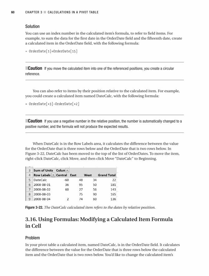
SolutionYou can use an index number in the calculated item’s formula, to refer to field items. Forexample, to sum the data for the first date in the OrderDate field and the fifteenth date, createa calculated item in the OrderDate field, with the following formula:

= OrderDate[1]+OrderDate[15]

■Caution If you move the calculated item into one of the referenced positions, you create a circularreference.

You can also refer to items by their position relative to the calculated item. For example,you could create a calculated item named DateCalc, with the following formula:

= OrderDate[+3]-OrderDate[+2]

■Caution If you use a negative number in the relative position, the number is automatically changed to apositive number, and the formula will not produce the expected results.

When DateCalc is in the Row Labels area, it calculates the difference between the valuefor the OrderDate that is three rows below and the OrderDate that is two rows below. InFigure 3-22, DateCalc has been moved to the top of the list of OrderDates. To move the item,right-click DateCalc, click Move, and then click Move “DateCalc” to Beginning.

Figure 3-22. The DateCalc calculated item refers to the dates by relative position.

3.16. Using Formulas: Modifying a Calculated Item Formula in Cell

ProblemIn your pivot table a calculated item, named DateCalc, is in the OrderDate field. It calculatesthe difference between the value for the OrderDate that is three rows below the calculateditem and the OrderDate that is two rows below. You’d like to change the calculated item’s


formula for one region, because it has missing data on one of the OrderDates. The exampleshown is from the DateCalc.xlsx workbook.

SolutionYou can modify the formula for an individual cell that contains a calculated item. For example,in the DateCalc calculated item, the index number was used to calculate the differencebetween two of the dates:

=OrderDate[+3]-OrderDate[+2]

If one of the columns has a blank cell for the date that is offset by 3, you can modify the for-mula to refer to the date that is offset by 4:

=OrderDate[+4]-OrderDate[+2]

To make the change, select the cell, and modify the formula in the formula bar (see Figure 3-23).

Figure 3-23. The calculated item’s formula is modified for one cell.

■Caution The Undo feature is not available after making this change, and the original formula will not berestored when the pivot table is updated. The modified cell’s formula will not be changed if the calculateditem’s formula is changed.

3.17. Using Formulas: Creating a Calculated Field

ProblemIn your pivot table, Rep and Product are in the Row Labels area. In the Values area, the Totalfield shows the total sales for each sales representative per product, and the Units field sum-marizes the number of units sold. You’d like to calculate a 3 percent bonus payable if a salesrepresentative has sold more than 100 units of any product. The example shown is from theOrderStatus.xlsx workbook.

SolutionTo calculate the bonus, you can create a calculated field. In a calculated field’s formula, youcan refer to other fields in the pivot table. In this example, you’ll test the Units field, to see ifmore than 100 units were sold, and multiply by the Total field.


1. Select any cell in the pivot table, and on the Ribbon, under the PivotTable Tools tab,click the Options tab.

2. In the Tools group, click Formulas, and then click Calculated Field.

3. Type a name for the calculated field, for example, Bonus.

4. In the Formula box, type =IF(Units>100,Total*3%,0).

5. Click OK to save the calculated field, and to close the dialog box. The Bonus fieldappears in the Values area of the pivot table, and in the field list in the PivotTable FieldList (see Figure 3-24).

Figure 3-24. The calculated field appears in the Values area.

■Note You can’t change the summary function for a calculated field. Sum is the only function available forthese fields.

3.18. Using Formulas: Modifying a Calculated Field

ProblemYou created a calculated field, and you’d like to change it. For example, in Section 3.17, abonus of 3 percent was calculated. Your company has increased the bonus to 5 percent, andyou need to calculate the new amounts. The example shown is from the OrderStatus.xlsxworkbook.

SolutionYou can go back into the Insert Calculated Field dialog box, and modify the settings.

1. In the pivot table, select any cell, and on the Ribbon, under the PivotTable Tools tab,click the Options tab.


3. From the Name drop-down list, select the name of the calculated field you want tomodify. In this example, the calculated field is named Bonus.


4. In the Formula box, change the formula. To increase the bonus percent, change the3 percent to 5 percent.

5. Click Modify, and then click OK to close the dialog box.

3.19. Using Formulas: Removing a Calculated Field

ProblemYou created a calculated field, and now you’d like to remove it from the pivot table layout.In this example, the calculated field is named Bonus. The example shown is from theOrderStatus.xlsx workbook.

SolutionYou can temporarily hide a calculated field, and then show it again later, or you can perma-nently remove the calculated field from the pivot table.

To temporarily remove a calculated field, follow these steps:

1. In the pivot table, right-click a cell in the calculated field.

2. Click Remove “Sum of Bonus.”

■Tip The calculated field is removed from the pivot table layout, but remains in the PivotTable Field List. Toadd the field to the layout later, add a check mark to the field in the PivotTable Field List.

To permanently remove a calculated field, follow these steps:

1. In the pivot table, select any cell, and on the Ribbon, under the PivotTable Tools tab,click the Options tab.


3. From the Name drop-down list, select the name of the calculated field you want todelete. In this example, the calculated field named Bonus is selected.

4. Click Delete, and then click OK to close the dialog box.

3.20. Using Formulas: Determining the Type of Formula

ProblemYour pivot table is complex, with many fields in the Row and Column Labels areas, and severalfields in the Values area. You can’t tell if a formula is a calculated item or a calculated field.


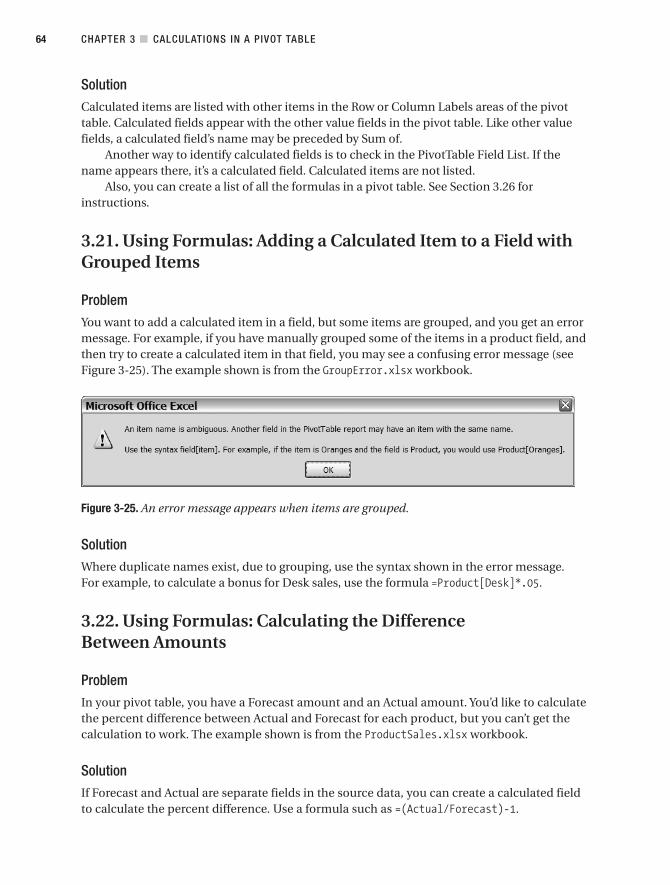
SolutionCalculated items are listed with other items in the Row or Column Labels areas of the pivottable. Calculated fields appear with the other value fields in the pivot table. Like other valuefields, a calculated field’s name may be preceded by Sum of.

Another way to identify calculated fields is to check in the PivotTable Field List. If thename appears there, it’s a calculated field. Calculated items are not listed.

Also, you can create a list of all the formulas in a pivot table. See Section 3.26 forinstructions.

3.21. Using Formulas: Adding a Calculated Item to a Field withGrouped Items

ProblemYou want to add a calculated item in a field, but some items are grouped, and you get an errormessage. For example, if you have manually grouped some of the items in a product field, andthen try to create a calculated item in that field, you may see a confusing error message (seeFigure 3-25). The example shown is from the GroupError.xlsx workbook.

Figure 3-25. An error message appears when items are grouped.

SolutionWhere duplicate names exist, due to grouping, use the syntax shown in the error message.For example, to calculate a bonus for Desk sales, use the formula =Product[Desk]*.05.

3.22. Using Formulas: Calculating the Difference Between Amounts

ProblemIn your pivot table, you have a Forecast amount and an Actual amount. You’d like to calculatethe percent difference between Actual and Forecast for each product, but you can’t get thecalculation to work. The example shown is from the ProductSales.xlsx workbook.

SolutionIf Forecast and Actual are separate fields in the source data, you can create a calculated fieldto calculate the percent difference. Use a formula such as =(Actual/Forecast)-1.


In the ProductSales.xlsx workbook, Forecast and Actual are items in the same field, so youcan use the % Difference From custom calculation. In Figure 3-26, Forecast and Actual are itemsin the Status field, and Sum of Units in the Values area shows the amount for each item. A secondcopy of the Units field was added to the Values area, and set to show the % Difference From, asdescribed in Section 3.5. For this calculation, Status is the base field, and Forecast is the base item.

Figure 3-26. Calculating the difference between amounts

3.23. Using Formulas: Correcting the Grand Total for aCalculated Field

ProblemYou have a calculated field that calculates a bonus based on each product’s orders:

=IF(Units>100,Total*5%,0)

You assume the grand total would be a sum of the bonus amounts, but it performs the samebonus calculation in the grand total row, creating the wrong total. The example shown is fromthe OrderStatus.xlsx workbook.

WorkaroundThe grand total for a calculated field performs the same calculation that’s defined in the calcu-lated field. As a workaround, you could use formulas outside the pivot table to extract the linetotals, and then sum those amounts (see Figure 3-27).

Finally, hide the pivot table column that contains the Bonus calculations, so only the col-umn with the correct Grand Total is visible.

Figure 3-27. The pivot table Grand Total is incorrect for the calculated field.


Or, if the pivot table layout won’t change, you could hide the Grand Total row, and thencreate formulas below the pivot table to total the columns.

3.24. Using Formulas: Calculated Field—Count of Unique Items

ProblemIn your pivot table, you want a count of unique products that have been ordered, but the Val-ues area only shows a count of orders. Some products appear in several orders, so the count oforders doesn’t tell you how many unique products were ordered. The example shown is fromthe ProdCount.xlsx workbook.

WorkaroundA pivot table won’t calculate a unique count. You could add a column to the source data, andthen add that field to the pivot table. For example, add a column in the source data, with theheading ProdCount. To count unique products in Column E, enter the following formula inrow 2 of the ProdCount column:

=IF(COUNTIF($E$1:E2,E2)=1,1,0)

Copy this formula down to the last row of data, and then add the ProdCount field to the pivottable Values area using the Sum function (see Figure 3-28).

Figure 3-28. Creating a unique count of products

How It WorksThe COUNTIF formula checks the range E1:E2 and counts the instances of the product nameentered in cell E2.

For the first occurrence of the name, the count is one. The IF formula checks the result ofthe COUNTIF formula, and if the count is one, the IF formula returns a one.

For the next occurrence of the product name, the COUNTIF formula would return a two.Because that is not equal to one, the IF formula would return a zero.

When you copy the formula down the column on the worksheet, only the first occurrenceof each product returns a one, so the sum of this column is the number of unique products.

In the formula, the reference to cell E1 is absolute ($E$1), so that reference does notchange as the formula is copied down the column in the source data. The other references, toE2, are relative, and change in each row, to refer to the cells in that row. The formula alwaysstarts its count in cell E1, and counts down to the row that contains the formula.


3.25. Using Formulas: Correcting Results in a Calculated Field

ProblemIn your source data, you have columns for cost and units, but the results are incorrect whenyou use a calculated field in the pivot table to multiply cost by units. The example shown isfrom the OrderStatus.xlsx workbook.

SolutionWhen you use a calculated field in the pivot table, the result is the Sum of Cost multiplied bySum of Units, and the result is inflated, except where the total number of units in a row is one.

Instead of using a calculated field, calculate the total cost (cost ✕ units) for each row inthe source data table. Then, add that field to the pivot table’s Values area to get the correcttotals.

3.26. Using Formulas: Listing All Formulas

ProblemYou’re documenting your workbook, and you would like to create a list of all the formulas forcalculated fields and calculated items you created in the pivot table.

Solution1. Select any cell in the pivot table, and then on the Ribbon, click the Options tab.

2. In the Tools group, click Formulas, and then click List Formulas.

A new sheet is inserted in the workbook, with a list of calculated items and a list of calculatedfields.

3.27. Using Formulas: Accidentally Creating a Calculated Item

ProblemYour pivot table contains a calculated item named Formula1, but you didn’t create one andaren’t sure how it got there. You’d like to delete the calculated item, and prevent it from hap-pening again. The example shown is from the CalcItem.xlsx workbook.

SolutionIt’s possible to accidentally create a calculated item if you select a cell that contains a Row orColumn label, and drag the fill handle, at the bottom right of the selected cell. Follow thesesteps to remove the formula:

1. Select the cell that contains the label for the Formula1 calculated item.

2. On the Ribbon, under the PivotTable Tools tab, click the Options tab.


3. In the Tools group, click Formulas, and then click Calculated Item.

4. From the drop-down list of formulas, select the formula you want to delete.

5. Click the Delete button, and then click the Close button.

3.28. Using Formulas: Solve Order

ProblemIn your pivot table, there are two calculated items:

CancelRate: = Cancel/(Cancel+Existing)All: East+West

In the pivot table, grand totals are hidden and the calculated items are shown (see the table atthe left in Figure 3-29). The example shown is from the SolveOrder.xlsx workbook. However,the CancelRate for All is incorrect. It’s a sum of the CancelRate for the individual regions(3.3%+2.5%), instead of a calculation of the CancelRate (3.2/(3.2+111.5)), based on the Alltotals.

You’d prefer to have the CancelRate for All be calculated like the CancelRate for the indi-vidual regions.

Figure 3-29. The pivot table, with two calculated items

SolutionYou can change the Solve Order for the calculated items to get the result you want:

1. Select a cell in the pivot table, and then on the Ribbon, click the Options tab.

2. In the Tools group, click Formulas, and then click Solve Order.

3. Select the All formula, and then click the Move Up button. Click Close.

The All CancelRate is adjusted and shows the All cancel ratio, instead of the sum of regionratios (see the table at the right in Figure 3-29).

■Note When you change the Solve Order, it affects all calculated items in the pivot table.


How It WorksCalculated items are added to the Solve Order list in the order in which they’re created. Forany result affected by two or more calculated items, the last calculation listed is the one thatdetermines its value.

In this example, the CancelRate calculated item was created first, and then the All calcu-lated item. The bottom-right cell in the pivot table is affected by both calculated items.

In the original Solve Order, the All calculated item is last in the Solve Order, so thebottom-right cell shows the result of that formula: East+West.

In the revised Solve Order, the CancelRate calculated item is last in the Solve Order, sothe bottom-right cell shows the result of that formula: Cancel/(Cancel+Existing).


Formatting a Pivot Table

New formatting features were introduced for pivot tables in Excel 2007, including PivotTableStyles, Document Themes, Conditional Formatting, and Report Layouts, which add manyexciting options for enhancing the look of your pivot tables. Questions about these new fea-tures are addressed in this chapter. Common problems with pivot table formatting includeloss of formatting when the pivot table is changed or refreshed, showing or hiding subtotalsand grand totals, and retaining formats applied in the source data.

Unless otherwise noted, the problems in this chapter are based on data in the sample filenamed Regions.xlsx.

4.1. Using PivotTable Styles: Applying a Predefined Format

ProblemYou create several pivot tables each week. Each pivot table has default formatting applied,and you spend time changing the colors and borders to match your company’s specifica-tions. You’d like a quick way to format your pivot table, so it easily coordinates with yourcompany’s other documents. This example is based on the Regions.xlsx workbook.

SolutionInstead of manually formatting a pivot table, you can apply one of the built-in PivotTablestyles, also called quick styles. Quick styles may affect the color and font formatting, andthey may add borders and row or column shading. Some styles include horizontal bordersor shading, which can make the rows easier to follow in a wide pivot table. Some styles havedramatic or dark colors that may be best suited for presentations or online viewing, ratherthan printing.

Follow these steps to apply a PivotTable style:

1. Select a cell in the pivot table, and on the Ribbon, click the Design tab. In the Pivot-Table Styles group, you can see one of the styles is selected, and it has a border aroundit. This is the style currently applied to your pivot table.

2. Point to one of the PivotTable styles, and the pivot table on the worksheet will show apreview of that style. Also, the style’s name should appear below the Ribbon, in aScreenTip (see Figure 4-1), unless you turned off the Screen Tips feature.

71

C H A P T E R 4

Figure 4-1. PivotTable styles

■Tip If the preview doesn’t show, you may have this feature turned off in the Excel Options. To turn thefeature on, click the Microsoft Office Button, click Excel Options, and in the Popular features, add a checkmark to Enable Live Preview.

3. To see other rows of PivotTable styles, click the up or down arrow at the right end of thePivotTable Styles group, or to open the full gallery of PivotTable styles, click the Morebutton, at the right end of the PivotTable Styles group (shown in Figure 4-1). In thegallery, you can drag the scroll bar up and down to see the PivotTable styles, whichare grouped as Light, Medium, and Dark.

■Tip If you change your mind, and don’t want to apply a style, press Esc on the keyboard, or click outsidethe Style gallery, and it will close without applying a style.

4. When you find a PivotTable style you like, click it, to apply that style to your pivot table.

■Tip To apply the selected style and remove any formatting manually applied to the pivot table, right-clickthe style, and then click Apply and Clear Formatting (this does not remove conditional formatting). If youdon’t use this option, the manual formatting is retained.

How It WorksWhen you select one of the PivotTable styles, it applies specific cell formatting to differentparts of the pivot table. For example, all the row subtotals may be changed to bold Calibri font,with blue fill color in the cell. If you change the pivot table layout, the formatting is retainedand adjusts to the new layout.

CHAPTER 4 ■ FORMATTING A PIVOT TABLE72

You can quickly modify the appearance of a built-in style by using the PivotTable StyleOptions. With these, you turn on or off the special formatting for the headers, rows, and col-umns. The Row Headers and Column Headers options apply or remove special fonts and fillcolors in the headers. The Banded Rows and Banded Columns apply or remove the shadingfrom rows and columns.

1. Select a cell in the pivot table, and on the Ribbon, click the Design tab.

2. In the PivotTable Style Options group, add or remove the check marks from the styleoptions (see Figure 4-2).

Figure 4-2. PivotTable Style Options

4.2. Using PivotTable Styles: Removing a PivotTable Style

ProblemYou applied a PivotTable style to a pivot table, and you would like to remove it. You would pre-fer to have a pivot table with no fill color or header formatting. This example is based on theRegions.xlsx workbook.

SolutionIn the PivotTable Styles gallery, you can apply a special style that removes the existing style,or you can use a command to clear the existing style. Follow these steps to clear a PivotTablestyle:


2. In the PivotTable Styles gallery, the first style, at the top left of the Light styles, is namedNone (see Figure 4-3). Click this style, and the existing style is removed. A thin borderremains around sections of the pivot table, and the gridlines, if displayed, are not visi-ble within the pivot table.

Figure 4-3. PivotTable style named None

CHAPTER 4 ■ FORMATTING A PIVOT TABLE 73

■Note When no PivotTable style is applied, the preview function won’t work when you point to a differentstyle in the PivotTable Styles gallery.

A different way to remove the PivotTable style is to click Clear, at the bottom left of thePivotTable Styles gallery (see Figure 4-4).

Figure 4-4. Clear a PivotTable style.

4.3. Using PivotTable Styles: Changing the Default Style

ProblemYou prefer one of the Dark PivotTable styles, and you apply it to almost every pivot table youcreate. You’d like to change the default PivotTable style, to save time when you create newpivot tables. This example is based on the Regions.xlsx workbook.

SolutionYou can change the default PivotTable style to one you prefer. Follow these steps to change thedefault:

1. Select a cell in the pivot table, and then on the Ribbon, click the Design tab.

2. In the PivotTable Styles gallery, right-click the style you want to set as the default, andin the context menu, click Set As Default.

This technique sets the default PivotTable style for the active workbook. If you want to makethis the default style for new workbooks, save the workbook as a template. Then, base newworkbooks on this template, and your default PivotTable style will be available.

4.4. Using PivotTable Styles: Creating a Custom Style

ProblemNone of the existing PivotTable styles has the exact formatting you need. You’d like to createyour own PivotTable style, with colors, borders, and fonts that match your company’s docu-ment specifications. This example is based on the Regions.xlsx workbook.


SolutionYou can create a custom PivotTable style with the formatting you require. If you find a Pivot-Table style close to what you need, you can duplicate that style, and modify the duplicate.

Follow these steps to create a custom style, based on an existing style:

1. Select a cell in the pivot table, and then on the Ribbon, click the Design tab.

2. In the PivotTable Styles gallery, right-click the style you want to duplicate.

3. In the context menu, click Duplicate. In this example, Pivot Style Medium 8 wasduplicated.

■Note If you don’t want to duplicate any style, click New PivotTable Style, at the bottom of the PivotTableStyles gallery, and then follow the next steps to name and modify the new style.

4. In the Modify PivotTable Quick Style dialog box, type a name for the new PivotTablestyle (see Figure 4-5). In this example, the name is My Gray Style.

Figure 4-5. Modify PivotTable Quick Style dialog box

■Tip Click a formatted Table Element, to view a description of its formatting in the Element Formattingsection of the Modify PivotTable Quick Style dialog box.


5. In the Table Element list, elements in bold font have formatting applied. You can mod-ify these, or clear their formatting. You can also select unformatted elements andformat them to meet your requirements. To modify an element’s formatting, click itto select it, and then click the Format button.

6. In the Format Cells dialog box, select the Font, Border, and Fill settings you want forthe selected element.

7. Click OK, to return to the Modify PivotTable Quick Style dialog box, where the format-ted element is listed with a bold font.

8. Repeat Steps 5 to 7, if required, to format other elements.

9. If you want your custom style to be the default PivotTable style, add a check mark toSet As Default PivotTable Quick Style For This Document.

10. Click OK, to close the Modify PivotTable Quick Style dialog box.

■Note The new PivotTable style is not automatically applied to the active pivot table.

The custom PivotTable Style you created is added to a Custom section of the PivotTableStyles gallery (see Figure 4-6). You can click the custom style there, to apply it to the activepivot table.

Figure 4-6. The Custom PivotTable styles on the Ribbon

4.5. Using PivotTable Styles: Copying a Custom Style toa Different Workbook

ProblemYou created several custom PivotTable Styles in a workbook, and you would like to copy thosestyles to other workbooks. You can’t find any command that will let you copy the styles from oneworkbook to another. This example is based on the Custom.xlsx and Regions.xlsx workbooks.

SolutionTo copy a custom PivotTable style to another workbook, you can apply that custom style to apivot table, and then temporarily copy that pivot table to a different workbook. Follow thesesteps to copy from the Custom.xlsx workbook to the Regions.xlsx workbook:


1. Select all the cells in a pivot table that has the custom style applied, and then on theRibbon’s Home tab, click Copy.

2. Switch to the workbook where you want the copy of the custom style, and then pastethe pivot table.

3. Delete the pasted copy of the pivot table.

The custom PivotTable style now appears in the PivotTable Styles gallery, and it can beapplied to any pivot table in the workbook.

4.6. Using Themes: Impacting PivotTable Styles

ProblemYou selected a different Document Theme in your workbook, and it changed the appear-ance of the worksheets and the styles in the PivotTable Styles gallery. You don’t understandhow Themes work, or why they affect the PivotTable styles. This example is based on theThemes.xlsx workbook.

SolutionEach Document Theme is a collection of colors, fonts, and visual effects you can share betweenExcel and other Office applications. You can use the existing themes, create new themes, ormodify the built-in themes.

To see what theme is currently applied, and what its settings are, you can view the Themeinformation on the Ribbon. Activate a worksheet that contains a pivot table, so you can seethe effect of theme changes.

1. On the Ribbon, click the Page Layout tab.

2. In the Themes group, point to the Themes command, and the tooltip then shows thename of the current theme.

3. To view the color palette for the current theme, in the Themes group, click Colors, toopen the color list. The current theme’s colors are surrounded by a thin border, to showthey are selected. If you point to a different theme’s colors, you can see the preview col-ors in your pivot table change.

4. A theme has two fonts: one for headings and one for body text. To view the fonts asso-ciated with the current theme, in the Themes group, click the Fonts command, to openthe list of fonts. The current theme’s fonts are selected, and show the Headings fontand the Body font. If you point to a different theme’s fonts, you can see the previewfonts in your pivot table change.

5. Finally, a theme also has effects that are used in charts and shapes, so if you createa PivotChart, its appearance will be affected by the current theme’s effects. To viewthe effects associated with the current theme, in the Themes group, click the Effectscommand, to open the list of effects. The current theme’s effects are selected, and theyshow the line thickness, fill type, and beveling that would be used for charts andshapes.


If you apply a different theme in your workbook, or modify the current theme, your pivottable’s appearance and PivotTable styles may be affected. The theme colors and fonts willoverride the settings in the PivotTable styles, and they could affect the way the pivot tableappears.

To apply a different theme, follow these steps:

1. On the Ribbon, click the Page Layout tab.

2. In the Themes group, click Themes, and then in the Themes gallery, click the themeyou want to apply.

The colors and fonts in your file will change, and your pivot table and Excel Table may bewider or narrower, if the fonts are much different. In the Themes group on the Page Layouttab, the icons have changed, to reflect the colors, fonts, and effects of the current theme. In thePivotTable Styles gallery, the styles use the colors from the new theme. Even the font in therow and column buttons changes to the Body font for the current theme.

4.7. Using the Enable Selection Option

ProblemIn your pivot table, the Region and City fields are in the Row Labels area. You want to use adifferent font size for the Region subtotals, and you’d like to select and format all the subto-tals at the same time, instead of formatting each one separately. This example is based on theRegions.xlsx workbook.

SolutionIf the subtotals are at the bottom of the group, in either the Row Labels area or the ColumnLabels area, you can select them all, and then format them together. To select them, you mayhave to activate the Enable Selection option.

1. Select a cell in the pivot table, and on the Ribbon, click the Options tab.

2. In the Actions group, click Select, and then check to see if Enable Selection is activated(see Figure 4-7).

Figure 4-7. The Enable Selection option turned on

3. If Enable Selection isn’t activated, click it to activate the feature. If it is activated, clickthe worksheet, to close the menu without making a selection.

4. To select subtotals for a Row Labels field, point to the left edge of a cell that contains asubtotal label, and when the pointer changes to a black arrow shape (see Figure 4-8),click to select all the subtotals for that field.


Figure 4-8. The black arrow pointer at the left of the subtotal in Row 8

5. If the subtotals are for a Column Labels field, point to the top edge of a cell that con-tains a subtotal label, and when the pointer changes to a black arrow shape, click toselect all the subtotals for that field.

6. Format the selected subtotals, using the commands on the Ribbon’s Home tab.

4.8. Losing Formatting When Refreshing the Pivot Table

ProblemYou manually adjusted the column widths and applied formatting to the cells in your pivottable. However, your pivot table formatting is lost when you refresh the pivot table or changethe pivot table layout. Even changing the report filter causes the formatting to be lost. Thisexample is based on the LoseFormat.xlsx workbook.

SolutionMost formatting can be preserved if you change the Format options in the PivotTable Optionsdialog box.

1. Right-click a cell in the pivot table, and then choose PivotTable Options.

2. On the Layout & Format tab, in the Format options, remove the check mark fromAutofit Column Widths on Update. This prevents the column width from changing,if you have manually adjusted it.

3. Add a check mark to Preserve Cell Formatting on Update, and then click OK.

Then, when you apply formatting, do the following:

1. Ensure that Enable Selection is turned on (as shown in Figure 4-7).

2. Unless you want to format a single cell, use the pivot table selection technique to selectthe elements you want to format (point to the top or left edge of the element, and thenclick when the black arrow appears).

4.9. Hiding Error Values on Worksheet

ProblemErrors, such as #N/A, are in the Excel Table on which the pivot table is based, and you’d like tohide them in the pivot table. This example is based on the Errors.xlsx workbook.


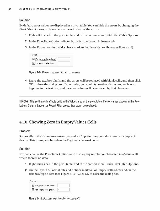
SolutionBy default, error values are displayed in a pivot table. You can hide the errors by changing thePivotTable Options, so blank cells appear instead of the errors:


2. In the PivotTable Options dialog box, click the Layout & Format tab.

3. In the Format section, add a check mark to For Error Values Show (see Figure 4-9).

Figure 4-9. Format option for error values

4. Leave the text box blank, and the errors will be replaced with blank cells, and then clickOK to close the dialog box. If you prefer, you could type other characters, such as ahyphen, in the text box, and the error values will be replaced by that character.

■Note This setting only affects cells in the Values area of the pivot table. If error values appear in the RowLabels, Column Labels, or Report Filter areas, they won’t be replaced.

4.10. Showing Zero in Empty Values Cells

ProblemSome cells in the Values area are empty, and you’d prefer they contain a zero or a couple ofdashes. This example is based on the Regions.xlsx workbook.

SolutionYou can change the PivotTable Options and display any number or character, in a Values cellwhere there is no data:


2. On the Layout & Format tab, add a check mark to For Empty Cells, Show and, in thetext box, type a zero (see Figure 4-10). Click OK to close the dialog box.

Figure 4-10. Format option for empty cells


4.11. Hiding Buttons and Labels

ProblemYou’re sending your pivot table to a colleague, and you want to hide some of the buttons andfilter drop-downs in the pivot table before you send it. Your colleague isn’t too familiar withpivot tables, and you want to make it look as simple and uncluttered as possible. This exampleis based on the Regions.xlsx workbook.

SolutionYou can change the Pivot Table Options to hide some of the buttons and captions in the pivottable. Follow these steps to hide some of the features:

1. Right-click a cell in the pivot table and, in the context menu, click PivotTable Options.

2. On the Display tab, remove the check mark from Show Expand/Collapse Buttons. Thishides the buttons to the left of the outer Row Labels and Column Labels.

3. Also remove the check mark from Display Field Captions and Filter Drop Downs. Thishides the filter buttons, as well as the Row Labels and Column Labels captions.

4. Click OK to close the PivotTable Options dialog box.

4.12. Applying Conditional Formatting: Using a Color Scale

ProblemYou’ve created a pivot table report to send to the store managers. Your pivot table is a denseblock of numbers, with the Product field in the Row Labels area, the Store field in the ColumnLabels area, and the TotalPrice field in the Values area. You’d like to color the Values cells, tohighlight the highest and lowest values.

Instead of reading all the numbers, the store managers could quickly identify the prod-ucts and stores with the strongest sales because cells that contain those values would becolored green. The products and stores with the weakest sales would have values in red cells—a signal for trouble! The reasons for those low sales could be investigated. This example isbased on the Stores.xlsx workbook.

SolutionYou can use conditional formatting to add visual impact to the data in a pivot table, just aswith other cells in the workbook. To quickly format the cells in a pivot table, you can use oneof the built-in color scales.

Follow these instructions to add a conditional formatting color scale to a pivot table witha single block of cells to format.


1. In the pivot table Values area, select the cells you want to color. In the sample file,select cells B5:E15.

■Caution Do not include the Grand Total rows or columns, or they will be colored as the highest values.

2. On the Ribbon, click the Home tab, and in the Styles group, click ConditionalFormatting.

3. In the list of conditional formatting options, click Color Scales, and then click the firstoption—Green-Yellow-Red Color Scale.

■Tip In the Color Scales menu, point to any of the color scale options to see a preview of the formatting onthe selected cells.

How It WorksIn a three-color scale, the cells with the lowest, median, and highest values are a solid color,and cells with values in between have a graduated color. In the Green-Yellow-Red color scale,the cell with the highest value is solid green, the cell with the median value is solid yellow, andthe cell with the lowest value is solid red.

Two-color scales, which use one color for the cell with the highest number, and a secondcolor for the cell with the lowest number, are also available. Cells with values between thehighest and lowest are shaded in a graduated color scale.

■Note Cells with no data will not be formatted.

4.13. Applying Conditional Formatting: Using an Icon Set

ProblemYour pivot table has a list of sales totals for each product, and instead of numbers, you’d like toshow traffic lights, to indicate the high, low, and middle results. This can create a simple reportyou can share with employees, without disclosing all the numbers. This example is based onthe Products.xlsx workbook.


SolutionYou can use conditional formatting icon sets to illustrate the data. These small pictures useshapes and colors to mark the values. There is a wide variety of icon sets, including trafficlights, with red for low, yellow for middle, and green for high results.

1. In the pivot table, select the cells where you want to add icons. In the sample file,select cells B4:B14.

2. On the Ribbon, click the Home tab, and in the Styles group, click ConditionalFormatting.

3. In the list of conditional formatting options, click Icon Sets, and then click one of thetraffic light options. For example, click the 3 Traffic Lights (Unrimmed) option.

■Tip Point to any of the icon-set options to see a preview of the formatting on the selected cells.

The icon set is added to the cell, to the left of the numbers. To remove the numbers fromthe cells, so only the icons are visible, you can adjust the settings for the conditional format-ting you applied. Follow these instructions to remove the numbers from the cells:

1. In the pivot table, select the cells that contain the icon set, and on the Ribbon, click theHome tab, and then in the Styles group, click Conditional Formatting.

2. In the list of conditional formatting options, click Icon Sets, and then click More Rules,at the bottom of the list of Icon Sets.

3. In the New Formatting Rule dialog box, the current settings for the icon set are dis-played. At the bottom right, add a check mark to Show Icon Only, and then click OK(see Figure 4-11). You can use the Alignment options on the Ribbon’s Home tab to cen-ter the icons in the cells.

Figure 4-11. Show Icon Only


■Tip In the New Formatting Rule dialog box, you can also adjust the settings for the icons, to control whichpercent of values have one of the icons. You can also check the Reverse Icon Order option, to change theorder in which the icons are applied. This option is useful if high numbers indicate a poor result, and youwant them red, instead of green.

4.14. Applying Conditional Formatting: Using Bottom 10 Items

ProblemYou’re preparing a report for a sales meeting, and you’d like to highlight only the bottomtwo results in a list of product sales. You don’t want to use a color scale that will color all theselected cells, because you want the discussion to focus on only the lowest results. This exam-ple is based on the Bottom.xlsx workbook.

SolutionTo highlight just the lowest results, you can use the Bottom 10 Items conditional formattingoption. The other options in the Top/Bottom Rules list work similarly, and you can select theseto highlight the top or bottom items or percent, or cells with above or below average values.

Follow these instructions to highlight the bottom two results in the selected cells, usinga custom format:

1. In the pivot table, select the cells you want to format, and on the Ribbon, click theHome tab, and then in the Styles group, click Conditional Formatting.

2. In the list of conditional formatting options, click Top/Bottom Rules, and thenclick Bottom 10 Items. The Bottom 10 Items dialog box opens, with ten as the set-ting in the scroll box at the left. The default formatting option, Light Red Fill withDark Red Text, is selected in the drop-down list at the right. The selected cells showa preview of this formatting, and you can change either of the settings to meet yourrequirements.

3. In the scroll box, change the number of items to two.

You can select a formatting option from the drop-down list or create a customformat.

4. Click the drop-down arrow to open the formatting list, and then click Custom Format,to open the Format Cells dialog box.

5. In the Format Cells dialog box, select the Number, Font, Border, and Fill options youwant for the highlighted cells.


■Note Some formatting options, such as font size or thick borders, are unavailable, because conditionalformatting doesn’t allow settings that could affect the cell size.

6. Click OK, to close the Format Cells dialog box, and then click OK to close the Bottom10 Items dialog box.

■Note In the case of a tie, more than the specified number of cells may be formatted.

4.15. Applying Conditional Formatting: Formatting CellsBetween Two Values

ProblemThe sales manager wants to run a promotion at stores with sales between 500 and 1000. Inyour pivot table report, you’d like any cell that contains a value in this range to be coloredgreen, to stand out from the other amounts. Next week, the target values may change, so you’dlike it to be easy to change the formatting criteria. This example is based on the Between.xlsxworkbook.

SolutionTo highlight cells within a specific range of values, you can use the Highlight Cell Rulesconditional formatting option. To make this formatting more flexible, you can type theminimum and maximum amounts on the worksheet, and refer to those cells in the condi-tional formatting.

1. In an empty cell in the workbook, type the minimum amount for the conditional for-matting, and in another cell, type the maximum amount. In the sample workbook, thevalues are typed in cells E1 and F1.

2. In the pivot table, select the cells you want to format, and on the Ribbon, click theHome tab, and then in the Styles group, click Conditional Formatting.

3. In the list of conditional formatting options, click Highlight Cells Rules, and then clickBetween.

4. Delete the default value in the minimum box, and click the cell that contains the mini-mum value you typed. Delete the default value in the maximum box, and click the cellthat contains the minimum value you typed on the worksheet (see Figure 4-12).


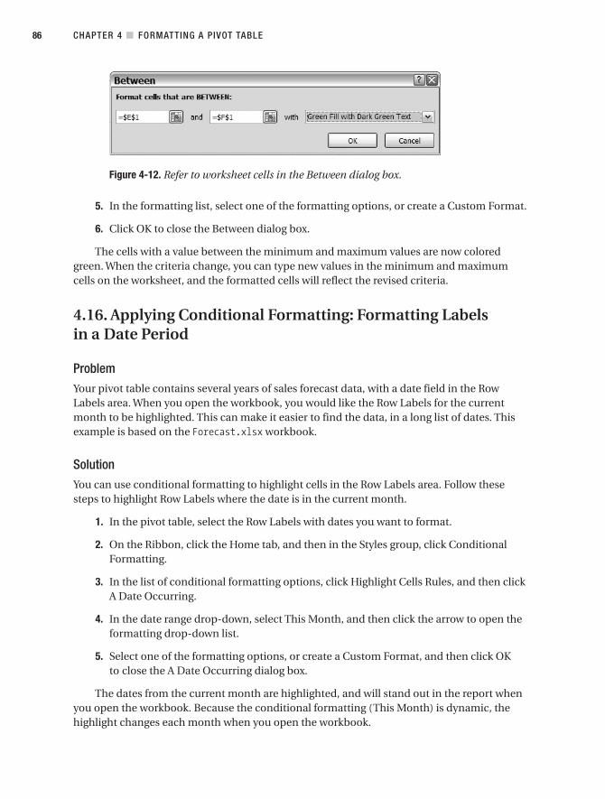
Figure 4-12. Refer to worksheet cells in the Between dialog box.

5. In the formatting list, select one of the formatting options, or create a Custom Format.

6. Click OK to close the Between dialog box.

The cells with a value between the minimum and maximum values are now coloredgreen. When the criteria change, you can type new values in the minimum and maximumcells on the worksheet, and the formatted cells will reflect the revised criteria.

4.16. Applying Conditional Formatting: Formatting Labelsin a Date Period

ProblemYour pivot table contains several years of sales forecast data, with a date field in the RowLabels area. When you open the workbook, you would like the Row Labels for the currentmonth to be highlighted. This can make it easier to find the data, in a long list of dates. Thisexample is based on the Forecast.xlsx workbook.

SolutionYou can use conditional formatting to highlight cells in the Row Labels area. Follow thesesteps to highlight Row Labels where the date is in the current month.

1. In the pivot table, select the Row Labels with dates you want to format.

2. On the Ribbon, click the Home tab, and then in the Styles group, click ConditionalFormatting.

3. In the list of conditional formatting options, click Highlight Cells Rules, and then clickA Date Occurring.

4. In the date range drop-down, select This Month, and then click the arrow to open theformatting drop-down list.

5. Select one of the formatting options, or create a Custom Format, and then click OKto close the A Date Occurring dialog box.

The dates from the current month are highlighted, and will stand out in the report whenyou open the workbook. Because the conditional formatting (This Month) is dynamic, thehighlight changes each month when you open the workbook.


4.17. Applying Conditional Formatting: Using Data Bars

ProblemYou’ve created a pivot table to summarize sales for the past two years. The Date field is in theRow Labels area, grouped by Month, and the Sales field is in the Values area. The pivot tablewill be used in a slide presentation, and you’d like to make it easy to visually compare the totalsales for each month. This example is based on the DataBars.xlsx workbook.

SolutionIn a list of values, you can use conditional formatting to add data bars to the value cells. Thiscan make it easy to visually compare the list of numbers, to see which months have the small-est numbers, and which months have the largest. Follow these instructions to add data bars tothe pivot table.

■Tip Color scales, icon sets, and data bars can all be applied simultaneously to the cells. However, usingmore than one of the conditional formatting options may add confusion to the pivot table, rather than helpillustrate the data, and using a single type is best in most cases.

1. In the pivot table, select the value cells you want to format. Don’t include the GrandTotal value, because you only want to compare the individual months. In the samplefile, select cells B4:B9.

2. On the Ribbon, click the Home tab, and then in the Styles group, click ConditionalFormatting.

3. In the list of conditional formatting options, click Data Bars, and then click one of theData Bar options. The Data Bar options are identical, except for the color.

■Tip If you find it difficult to see where the bars end, because of the graduated coloring in the data bars,you can apply a dark fill color to the cells, and then change the font to a light color.

How It WorksThe conditional formatting data bars aren’t exactly like using a bar chart. The data bars are notzero-based; the shortest data bar represents the lowest value in the formatted data, and thelongest bar represents the highest value in the formatted data.

If the lowest value is zero, and the highest value is 50, the data bars might look thesame as the data bars for data with values that ranged from 500 to 3000, or values from-3000 to -500 (see Figure 4-13). Even if the lowest value is zero, or a negative number, itis represented by a small data bar.


Figure 4-13. Data bars appear the same for different sets of values.

In this example, the lowest month is June, with 621 sales, and the highest month is Janu-ary, with 1277 (see Figure 4-14). Although the lowest number is approximately one half of thehighest number, its bar appears to be about one tenth the length of the longest bar. This exag-gerates the difference between the values.

Figure 4-14. Data bars and numbers

You can modify the conditional formatting, to fix the scale of the data bars.

1. In the pivot table, select the cells that contain the formatted value cells.

2. On the Ribbon, click the Home tab, and in the Styles group, click Conditional Format-ting, and then click Manage Rules.

3. The Conditional Formatting Rules Manager dialog box opens, where you can see theData Bar rule, and any other conditional formatting rules in the pivot table. In the listof rules, click your Data Bar rule.

4. Click the Edit Rule button, to open the Edit Formatting Rule dialog box.

The first section of the Edit Formatting Rule dialog box shows where the rule is applied.The second section shows the type of rule that was applied. In the third section, Edit the RuleDescription, you can see the current settings for the Data Bar rule, and this is where you editthe rule. No changes are required in the first or second section.

You want to ensure the amounts are accurately represented in the data bars, so youchange the settings for the Shortest Bar. Instead of using the lowest value in the range of cells,you use zero as the setting for the Shortest Bar.


1. Click the arrow for the Type drop-down list, under Shortest Bar (see Figure 4-15).

Figure 4-15. Type options for Shortest Bar

2. Click Number, and a zero automatically appears in the Value box, for the Shortest Bar.This is the setting you want, so leave the Value as zero.


The data bars now use a scale from zero to the highest number, to show a more accuraterepresentation of the numbers.

4.18. Applying Conditional Formatting: Changing theData Range

ProblemIn your pivot table, Date is in the Row Labels area, Territory is in the Column Labels area, andSales is in the Values area. You applied Above Average conditional formatting to the Valuescells, and it is working as expected. The sales manager has asked for a last-minute change tothe pivot table layout, and he would like you to show the product sales for each date.

You added the Product field to the Column Labels area, and moved Territory to the RowLabels area, above the Date field. Now the Grand Totals column is formatted, as well as theValues cells. The sales meeting will start soon, and you need to fix the problem. This exampleis based on the Territory.xlsx workbook.

SolutionWhen you select a block of cells in the pivot table, and then apply conditional formatting, theformatting rule is applied to those cells. If you change the pivot table layout, the formattingrule may adjust correctly and continue to format the cells as intended. However, after somelayout changes, the rule may be applied to the wrong cells, especially if additional fields areadded to the layout. Follow these instructions to change the conditional formatting range fora rule.


1. Select a cell in the pivot table, and on the Ribbon, click the Home tab.

2. In the Styles group, click Conditional Formatting, and then click Manage Rules. TheConditional Formatting Rules Manager dialog box opens, where you can see the rulesthat exist for the active pivot table. For each rule, the list shows where the conditionalformatting is applied. You can change this setting, to ensure the conditional formattingcontinues to work as expected, if the pivot table layout changes.

3. In the list of rules, click the Above Average rule.

4. Click the Edit Rule button, to open the Edit Formatting Rule dialog box. In the ApplyRule To section at the top, there are three options, and the Selected Cells option is cur-rently selected. The current range of cells where the formatting is applied is shown(see Figure 4-16).

Figure 4-16. Apply Rule To options in the Edit Formatting Rule dialog box

• The Selected cells option works in many cases, but when you rearrange the pivottable, the conditional formatting may not adjust correctly. In your pivot table,incorrect cells may be formatted because they are within the range of cells towhich the rule is applied.

• In this example, the second option, All Cells Showing “Sum of Sales” Values, mightalso include too many cells, such as subtotals, and Grand Totals.

• The third option, All Cells Showing “Sum of Sales” Values for “Date” and “Product,”is the best option for this pivot table. It restricts the formatting to cells where theDate and Product values appear, and it excludes the subtotals and the Grand Totals.

5. Select the third option, All Cells Showing “Sum of Sales” Values for “Date” and“Product.”

6. Click OK, twice, to close the two dialog boxes.

The conditional formatting is now applied correctly, to the individual value cells. TheGrand Total cells are not formatted, and their values are not included in the average calcula-tion. You can send the modified report to the sales manager, and go for a well-earned lunchbreak before the meeting starts.


4.19. Applying Conditional Formatting: Changing the Orderof Rules

ProblemIn your pivot table, you created a conditional formatting rule to color the top three salesamounts, using bold font and green fill color. You also created a conditional formatting rule tocolor the above-average sales, using yellow fill color. Now, the top three sales amounts havebold font, but the cells are yellow, instead of green. This example is based on the Order.xlsxworkbook.

SolutionConditional formatting rules are applied in a specified order, and if a cell meets the criteria formultiple conflicting rules, it uses the formatting from the last rule. You can control the rulesorder, and move rules up or down in the list. Follow these instructions to change the rulesorder, so the Top 3 rule is applied last.


2. In the Styles group, click Conditional Formatting, and then click Manage Rules.

The Conditional Formatting Rules Manager dialog box opens, where you can see the tworules you created (see Figure 4-17).

Figure 4-17. Two rules in the Conditional Formatting Rules Manager dialog box

When you create a new rule, it goes to the top of the rules list, and has precedence overthe other rules. If a formatting conflict occurs, the formatting for the rule with precedence isapplied.

You created the Top 3 rule first, so it’s at the bottom of the list. When you created theAbove Average rule, it was added to the top of the list, taking precedence over the Top 3 rule.Because the Top 3 cells are also Above Average, they are affected by both rules, and the AboveAverage rule, which has precedence, is applied last, so the cells are colored yellow. No conflictis in the font formatting, however, so the bold formatting remains visible.

You can change the order of the rules, so the Top 3 rule has precedence, and then thegreen fill color is applied to the Top 3 cells.


1. In the list of rules, click the Top 3 rule.

2. Click the Move Up button (to the right of the Delete Rule button), to move the Top 3rule above the Above Average rule.

3. Click OK, to close the Conditional Formatting Rules Manager dialog box.

Because you changed the order of the rules, the Top 3 rule now has precedence, and theTop 3 cells are colored green, with bold font.

4.20. Removing Conditional Formatting

ProblemYou applied conditional formatting to the cells in your pivot table, and now the sales man-ager has asked you to remove it. You’d like to remove the conditional formatting, withoutaffecting any of the other formatting in the pivot table. This example is based on theOrder.xlsx workbook.

SolutionAfter applying conditional formatting, you can remove it if it’s no longer required. You canchoose to remove it from the selected cells, the entire sheet, or the active pivot table. Followthese steps to remove all the conditional formatting from the active pivot table:


2. In the Styles group, click Conditional Formatting.

3. Click Clear Rules, and then click Clear Rules from This PivotTable.

■Note If you want to remove conditional formatting from only specific cells, select those cells, and thenuse the Clear Rules from Selected Cells command.

4.21. Creating Custom Number Formats in the Source Data

ProblemThe lab sent you a workbook with test results, and you created a pivot table to summarize thedata by week. Some numbers in the data have a symbol—for example, <0.1—and those num-bers aren’t showing up in the pivot table. This example is based on the TestResults.xlsxworkbook.

SolutionIf symbols such as < (less than) and > (greater than) are typed in the source data, they changethe numbers into text. In the pivot table, text is displayed as zero in the Values area.


You could create a custom number format, and then apply that format to the source data,instead of using typed symbols, and the values would be totaled correctly in the pivot table.

1. In the source data, enter the actual values, instead of <0.1.

2. Select the cells you want to format, right-click one of the selected cells, and in the con-text menu, click Format Cells.

3. On the Number tab, select the Custom category.

4. In the Type box, type [<0.1] <0.1";General (see Figure 4-18). The custom number for-mat has two sections, separated by a semicolon. In the first section, [<0.1] is thecondition to use to test the numbers. In this case, numbers less than 0.1 receive specialformatting. The text in quotation marks, <0.1", is the formatting the qualifying num-bers receive. In the second section, General specifies how any other numbers will beformatted.

Figure 4-18. Enter a Custom Format Type.

5. Click OK, to close the dialog box.

6. To have this format appear in the pivot table, you can apply the custom number for-mat to the values.

4.22. Changing the Report Layout

ProblemYou’d like to change the pivot table layout so it looks like a pivot table from earlier versionsof Excel, with each Row Label field in a separate column. You prefer this format, and you’dlike to see the Row Label field names at the top of each column. This example is based onthe RegionFood.xlsx workbook.

SolutionInstead of the default Compact Form, you can apply a different Report Layout, and the pivottable will have the same structure it had in earlier versions of Excel.


2. In the Layout group, click Report Layout, and then click either Show in Outline Form orShow in Tabular Form.


How It WorksIn Outline Form, each Row Label item is on a separate row, and each Row Label field is ina separate column. The labels for the outer fields are always above the labels for the relatedinner fields, and the subtotals can be at the top or the bottom of the group.

In Tabular Form, each Row Label field is in a separate column. The labels for the outerfields are on the same row as the first label for the related inner fields, and the subtotals canonly be shown at the bottom of the group (see Figure 4-19).

■Note Your pivot table may have different borders or fill color, depending on the PivotTable style youapplied. To hide some lines within the pivot table in Tabular layout, turn off Gridlines, on the Ribbon’s View tab.

Figure 4-19. Comparing Outline Form (left) and Tabular Form (right)

4.23. Increasing the Row Labels Indentation

ProblemYour pivot table is in the default Compact Form report layout. When you add fields to theRow Labels area, each additional field is indented from the field above it. You would like toslightly increase the indentation, to make the labels easier to read. This example is based onthe Regions.xlsx workbook.

SolutionYou can change a pivot table option, to increase the number of characters in the indentation.


2. On the Layout & Format tab, in the Layout section, increase the number of charactersin the setting—When in Compact Form Indent Row Labels 1 Character(s). You can setthe indent for up to 127 characters, but with that setting, it’s not really a compact form!



4.24. Repeating Row Labels

ProblemWhen you apply the Outline Form or Tabular Form layout to your pivot table, the Row Labelsonly appear in the first row for each Region. You would like a label to appear in each row, soyou can export the pivot table data for use with other programs (see Figure 4-20). This exam-ple is based on the RegionFood.xlsx workbook.

Figure 4-20. Row Labels in first row only (left) and repeating (right)

WorkaroundThe row labels show only once in a pivot table, and there’s no setting you can change to forcethem to repeat. If you need to export a copy of the pivot table with a heading in each row, youcan make a copy of the pivot table and repeat the headings there.

In the following steps, you copy the pivot table, select the blank cells, and then create aformula to copy the value from the row above. Finally, you can change the formulas to values.

1. With the pivot table in Tabular Form Layout, select all the cells in the pivot table, andon the Ribbon’s Home tab, click Copy.

2. Right-click the cell where you want to paste the copy, and in the context menu, clickPaste Special, then click Values, and then click OK.

3. In the copied pivot table, select the cells that contain the Row Labels, and the blankcells below them, where you want the labels repeated.

4. On the Ribbon, click the Home tab, and in the Editing group, click Find & Select, andthen click Go To Special.

5. Select Blanks, and then click OK.

6. Type an equal sign, and then press the up arrow on the keyboard—this enters a refer-ence to the cell above.

7. Press Ctrl+Enter—this enters the formula in all selected cells.

If you plan to sort the data, follow these steps to change the formulas to values. This pre-vents the formula results from changing if the cells move.


1. In the copied pivot table, select all the row labels, and then copy them.

2. On the Ribbon, click the Home tab, click the lower section of the Paste command, andthen click Paste Values.

■Caution Use Paste Special Values with caution if other cells are in the range that contain formulas.

4.25. Separating Field Items with Blank Rows

ProblemTo make the pivot table easier to read, you’d like each outer row field item to be followed by ablank row. When you try to insert rows in the pivot table, you get an error message that saysyou cannot insert rows. This example is based on the Regions.xlsx workbook.

SolutionIn any of the Report Layouts, you can format the outer row fields, so each item has a blank rowafter it. All the outer row fields will be affected by this setting.


2. In the Layout group, click Blank Rows, and then click Insert Blank Line After Each Item.

■Tip You can’t enter text in the blank row, but you can manually format the row—for example, add a fillcolor to visually separate the items, or you can format the blank rows as part of a PivotTable Style.

4.26. Centering Field Labels Vertically

ProblemYour pivot table is in the Tabular Form layout, and you’d like to center the field labels verticallyfor the outer fields in the Row Labels area of the pivot table. This example is based on theRegions.xlsx workbook.

Solution1. Right-click a cell in the pivot table, and then choose PivotTable Options.

2. On the Layout & Format tab, in the Layout section, add a check mark to Merge andCenter Cells with Labels.



This setting automatically centers the Row Labels vertically and horizontally. The subto-tals for the Row Labels, and the Grand Total row label are also centered vertically andhorizontally.

4.27. Changing Alignment for Merged Labels

ProblemYour pivot table is in Tabular Form layout, and you turned on the Merge and Center Cells withLabels option in the PivotTable Options dialog box. All the row labels are vertically and hori-zontally center-aligned, but you’d prefer them to be left-aligned. When you select a label celland try to change the alignment, you get an error message. This example is based on theRegions.xlsx workbook.

SolutionEnsure that Enable Selection is turned on, and click at the top of a column of Row Labels, toselect all the labels for that field. Click the Align Text Left button on the Home tab of the Rib-bon, to change the alignment for all the selected labels.

■Note When the pivot table is refreshed or changed, the merged labels return to center alignment andhave to be reformatted.

4.28. Displaying Line Breaks in Pivot Table Cells

ProblemSome fields in your source data have line breaks (Alt+Enter). In the pivot table, these appearas a small square and question mark, instead of a line break. This example is based on theLineBreak.xlsx workbook.

SolutionIn the pivot table, format the cells with Wrap Text, to show the line break character:

1. In the pivot table, select the labels you want to have line breaks. In the sample file,select the City Row Labels.

2. On the Ribbon, click the Home tab, and in the Alignment group, click Wrap Text.


4.29. Freezing Heading Rows

ProblemYour pivot table is quite large and you want to keep the row and column headings visible asyou work. This example is based on the Long.xlsx workbook.

SolutionYou can freeze the cells at the top and left of the window, to keep those cells always in view.

1. Select the cell below and to the right of the cells you want to freeze. For example, tofreeze rows 1:5, and columns A:B, select cell C6. The selected cell can be inside yourpivot table.

2. On the Ribbon, click the View tab, and in the Window group, click Freeze Panes, andthen click Freeze Panes.

4.30. Applying Number Formatting to Report Filter Fields

ProblemYou want to change the date format of a field in the Report Filter area. When you right-click the date field label in the Report Filter area, and choose Field Settings, the NumberFormat button isn’t visible in the Field Settings dialog box. This example is based on theFilterFormat.xlsx workbook.

SolutionIf a numeric field in the source data contains blank cells, or cells with text, then the NumberFormat button won’t be displayed in the Field Settings dialog box for the pivot table field,except in the Values area. Fill the blank cells in the source data and remove any text, thenrefresh the pivot table, and then you’ll be able to format the pivot table field.

4.31. Displaying Hyperlinks

ProblemHyperlinks are in your source data, but when you add these fields to the pivot table, the hyper-links don’t appear. This example is based on the Hyperlinks.xlsx file.

WorkaroundThe pivot table can’t show hyperlinks from the source data, and you can’t add hyperlinks tothe pivot table. You could add a formula outside the pivot table, to create a hyperlink:

=IF(LEFT(A4,3)="www",HYPERLINK("http://"&A4),"")

but these formulas could be lost if the pivot table layout changes.


4.32. Changing Subtotal Label Text

ProblemThe Product field is the Row Labels area of your pivot table. You want to change the text insome of the Product subtotal labels to make them more descriptive, but when you type a newlabel, all the Product subtotal labels change to the same text. This example is based on theLabels.xlsx workbook.

SolutionIf you select a cell that contains a subtotal label and type a new label that doesn’t contain theitem name, each item subtotal in the field displays that same text in its label. For example, ifyou change a subtotal label from Bran Total to Grain Subtotal, every Product will have GrainSubtotal as its subtotal label.

However, if you include the item name in the revised label, then each item subtotalretains its unique identifier. For example, you can change the bran subtotal label from BranTotal to Subtotal—Bran. The subtotal for all other products shows the product name, pre-ceded by Subtotal.

■Caution These changes will not be undone if you reset the pivot table captions. You can type the originalversion of the subtotal text if you want to restore it.

4.33. Formatting Date Field Subtotal Labels

ProblemIn your pivot table, the OrderDate field is in the Row Labels area. You selected the date cells,and formatted them as dd-mmm-yy. When you added the Product field to the Row Labelsarea, the OrderDate subtotals used the mmm-yy date format, like the dates in the source datatable. You want the subtotals to use the dd-mmm-yy format. This example is based on theSubtotals.xlsx workbook.

SolutionWhen you format fields in the Row Labels area, change the formatting in the Field Settingsdialog box instead of selecting cells and changing the format.

1. Right-click one of the date field labels, and in the context menu, click Field Settings.

2. Click the Number Format button, and select the date formatting option you want.



4.34. Changing the Grand Total Label Text

ProblemOne field is in the pivot table’s Values area, and you would like to change the text in the GrandTotal labels. This example is based on the Labels.xlsx workbook.

SolutionYou can change all or part of the Row Grand Total text or the Column Grand Total text by typ-ing over the cell or editing in the cell or formula bar.

■Note If you change the label for either of these Grand Totals, the other automatically displays the revisedtext.

You can’t change the Row Grand Total text if multiple Values fields are arranged horizon-tally. You can’t change the Column Grand Total text if multiple Values fields are arrangedvertically.


Grouping and Totaling Pivot Table Data

When you add date fields to a pivot table, you can show the dates individually, or groupthem into larger units, such as years, quarters, or months. This adds flexibility to the pivottable, and enables you to do things like comparing the results from one year to another, orcreating a running total by quarter.

You can also group numeric fields, when you add them to the Row Labels or ColumnLabels area of the pivot table. By using this feature, you can group the numbers into largerchunks, such as groups of 10 or 25. If comparing test scores, or results by age, you can lookat larger segments of the population, instead of individual scores or ages.

It’s also possible to manually group text items in the Row Labels and Column Labelsareas, so you can group cities into a region, or employees into teams, and summarize thedata for the group.

Most of the time, grouping goes smoothly, but you may hit snags, or see error messageswhen you try to group the data in your pivot table. This chapter addresses those problems,and provides solutions or workarounds for the issues you might encounter.

This chapter also covers problems that may arise when summarizing pivot table resultsin subtotals and grand totals, and when summarizing fields in the Values area.

Except where noted, the problems in this chapter are based on the Stores.xlsx sampleworkbook.

5.1. Grouping: Error Message When Grouping Dates

ProblemYou created a pivot table with Category in the Column Labels area, Quantity in the Values area,and OrderDate in the Row Labels area. The sales manager would like the dates grouped bymonth, instead of seeing quantities for the individual dates.

This seemed like a simple request, but you get an error message, “Cannot group thatselection” (see Figure 5-1), when you right-click a date cell, and then click Group. This prob-lem is based on the GroupError.xlsx sample workbook.

101

C H A P T E R 5

Figure 5-1. This is the error message you see when items in a field can’t be grouped.

SolutionThis error occurs if there are cells that contain text, instead of dates, in the source data’sOrderDate field. For example, you may have entered text, such as N/A, if a date was not avail-able when the data was being entered. To correct the problem, you can do the following:

1. If any of the rows contain text, such as N/A, delete the text, or replace it with a date.

■Caution A blank cell does not cause problems with grouping, but use the Delete key to remove the text.Don’t type a space character.

2. Refresh the pivot table, and try to group the items in the date field.

3. If you’re still unable to group the dates, remove the date field from the pivot table lay-out, refresh the pivot table, and then add the date field to the pivot table again.

■Tip In the PivotTable Options dialog box, on the Data tab, if Number of Items to Retain Per Field is set toNone, you should be able to group the date field without following Step 3.

5.2. Grouping: Error Message When Grouping Numbers

ProblemThe logistics manager has asked for a report on the quantities per order. You created a reportwith Quantity in the Row Labels area, Category in the Column Labels area, and OrderDate inthe Values area, as Count of OrderDate. To simplify the report, you would like to show thequantities in groups of ten, such as 1–10, and 11–20, and show the number of orders in eachgrouping.

However, you get an error message that says, “Cannot group that selection,” when you tryto group the numbers. You checked the source data, and no text entries are in the Quantityfield. This problem is based on the GroupErrorNum.xlsx sample workbook.

CHAPTER 5 ■ GROUPING AND TOTALING PIVOT TABLE DATA102

SolutionSometimes, entries that look like numbers are not recognized as real numbers by Excel. Thenumbers may have been copied or imported from another program, and they are text valuesinstead of real numbers.

A quick way to test if the numbers are being recognized is to select two or more cells thatcontain numbers. Then, look in the status bar, at the bottom of the Excel window, to see if thenumbers show a Sum (see Figure 5-2). If only the Count is displayed in the status bar, thenumbers are stored as text.

Figure 5-2. The sum of selected cells shows in the status bar.

To correct the problem, you can do the following:

1. In the source data, convert the text to numbers, using one of the techniques describedin the following “How It Works” section.

2. After converting the text to numbers, refresh the pivot table, and then try to group thenumbers in the pivot table.

3. If you’re still unable to group the numbers, remove the number field from the pivottable layout, refresh the pivot table, and then add the number field to the pivot tableagain.

■Tip In the PivotTable Options dialog box, on the Data tab, if Number of Items to Retain Per Field is set toNone, you should be able to group the numbers without following Step 3.

How It WorksYou can convert text “numbers” to real numbers in several ways. For example, you can use thePaste Special command.

1. Select a blank cell in the workbook, and then copy it.

2. In the source data, select the cells that contain the text “numbers.”

CHAPTER 5 ■ GROUPING AND TOTALING PIVOT TABLE DATA 103

3. On the Ribbon, click the Home tab, and in the Clipboard group, click the lower sectionof the Paste command, and then click Paste Special (see Figure 5-3).

Figure 5-3. Paste Special command on the Ribbon

4. In the Paste Special dialog box, in the Operation section, select Add, and then click OK.

Another method for converting text numbers to real numbers is to use the Text toColumns feature.

1. Select the cells that contain the numbers you want to convert.

2. On the Ribbon’s Data tab, in the Data Tools group, click Text to Columns.

3. In the Convert Text to Columns Wizard, in Step 1, click Finish.

5.3. Grouping the Items in a Report Filter

ProblemYou added the OrderDate field to the Report Filter area, and a long list of dates is in the drop-down list. The sales manager frequently asks for a report for a specific month, so you wouldlike to group the dates by month, to make it easier to filter the report.

However, when you select the cell that contains the OrderDate drop-down list, the GroupField command on the Ribbon’s Options tab isn’t available. This problem is based on theStores.xlsx sample workbook.

WorkaroundYou can’t group the items in a field located in the Report Filter area. Temporarily move theOrderDate field to the Row Labels or Column Labels area and group the dates, and then movethe OrderDate field back to the Report Filter area.


5.4. Grouping: Error Message About Calculated Items

ProblemYou’re trying to group the dates in the OrderDate field, and you’re getting an error messagethat says, “You cannot add a calculated item to a grouped field” (see Figure 5-4). The Order-Date field doesn’t have any calculated items.

The only field with a calculated item is the Category field, and it’s not in the pivot tablelayout. This problem is based on the GroupErrorCalc.xlsx sample workbook.

Figure 5-4. Error message about calculated items

WorkaroundAlthough the OrderDate field has no calculated items, another field in the pivot table has acalculated item, and that’s preventing the grouping. Even though the other field is not visiblein the pivot table, it can still prevent the grouping.

■Tip When troubleshooting pivot table problems, it may help if you know what formulas are in the pivottable. To create a list of calculated items and calculated fields, select a cell in the pivot table, and on theRibbon’s Options tab, click Formulas, and then click List Formulas.

You can use one of the following workarounds:

• Delete the calculated item in the Category field, and then group the dates in the Order-Date field.

• Add a new field in the source data, with a formula to do the calculation, instead of usinga calculated item in the pivot table. Then, add the new field to the pivot table, anddelete the calculated item.

• Add a new field with formulas in the source data to create date groups. For example,add a new column with the heading “YearMonth” and use the following formula toshow the year and month, for a date in cell A2:

=TEXT(A2,"yyyy-mm")

Then, refresh the pivot table, and add the YearMonth field to the Row Labels area,instead of using the OrderDate field.


5.5. Grouping Text Items

ProblemThree new stores opened last year and the sales manager asked you for a report that comparesquantities sold in the new stores to sales in the older stores. You added the Store field to theRow Labels area of your pivot table, and you’d like to divide the stores into Old and New groups.The three lowest numbers are the older stores, and the three highest are the newer stores.

However, when you select a label in the Store field, the Group Field command on theRibbon’s Options tab isn’t available, so you aren’t sure how to create the groups. This problemis based on the Stores.xlsx sample workbook.

SolutionThe Group Field command is only available for date and number fields in the Row Labels orColumn Labels area of the pivot table. Because the store numbers are entered as text, andthat’s how you want them to remain, you can use the following method to group the stores.

1. Manually select the stores you want in the first group. To select nonadjacent stores,hold the Ctrl key, and then click the store numbers. In the sample file, select stores3000, 3036, and 3062.

2. On the Ribbon’s Options tab, click Group Selection (see Figure 5-5).

Figure 5-5. Group Selection command

This creates a group named Group1, with the selected stores listed under that heading(see Figure 5-6). For each of the remaining stores, a heading is created, with its storenumber.

Figure 5-6. Group1 created in the Row Labels area

3. Select the Group1 heading, and then type a name for the group, such as Old.

4. Select the remaining stores, and click the Group Selection command to group them.Name the second group as New.


■Tip To select the remaining stores, drag down through the list of store numbers in the Row Labels area.You can include the store number headings that were created.

As an alternative to grouping the stores in the pivot table, you could add a StoreTypefield to the source data, and then enter Old or New for each record. Add the StoreType fieldas the first field in the Row Labels area and the stores will appear under the correct Store-Type heading.

5.6. Grouping Dates by Month

ProblemYour pivot table is based on two years of sales data. When you group the order dates in yourpivot table by month, the January data from both years is lumped together. You’d like to keepthe data from different years separated, so you can compare the monthly data between years.This problem is based on the GroupMonth.xlsx sample workbook.

SolutionWhen you group the dates, select both Year and Month in the Group By list. With this type ofgrouping, data from each year is grouped, and within each year, the data for each month isgrouped.

A Years field is automatically added to the PivotTable Field List, and you can move it to adifferent area of the pivot table. For example, you could move Years to the Report Filter area,and leave the OrderDate field, showing Months, in the Row Labels area.

5.7. Grouping Dates Using the Starting Date

ProblemYou want to group the order dates into four-week periods that coincide with your sales calen-dar. You successfully group the dates, but the date ranges are a couple of days off, startingmidweek instead of on a Monday. This problem is based on the GroupStart.xlsx sampleworkbook.

SolutionWhen you group the dates, select to group by days, and set the number of days to 28. As astarting date, Excel automatically selects the first date in your source data, but you can enter adifferent date, to get the starting date you need.

For example, if the default starting date is Thursday, January 3, 2008, you could enterDecember 31, 2007 as the starting date for your grouping (see Figure 5-7). This forces all thegroupings to start on a Monday, and it matches the company’s sales periods.


Figure 5-7. Changing the starting date

5.8. Grouping Dates by Fiscal Quarter

ProblemYou added the OrderDate field to the Row Labels area of your pivot table, and you were able togroup the dates by year and quarter. However, you want to group the dates by your company’sfiscal quarter, which starts in July, instead of using the calendar quarter available in theGrouping dialog box. This problem is based on the GroupQtr.xlsx sample workbook.

WorkaroundThere’s no built-in option to group by fiscal quarter. In the source data, you can add a col-umn with a formula that calculates the fiscal quarter, and then add that field to the pivottable. For example, if your fiscal year starts in July, use the following formula to calculate thefiscal quarter:

=CHOOSE(MONTH(A2),3,3,3,4,4,4,1,1,1,2,2,2)

In the Choose formula, the first argument, Month(A2), returns the month of the date in cell A2.It uses that number to select the appropriate fiscal quarter number from the numbers that fol-low. For example, if the month is April, the month number is 4. In the Choose formula, thefourth number is 4, so that is the fiscal quarter in which April falls.

In another column, you can also calculate the fiscal year. For example, if fiscal year 2009starts in July 2008:

=YEAR(A2)+(MONTH(A2)>=7)

Refresh the pivot table, and then ungroup and remove the OrderDate field. Add the fiscal yearand fiscal quarter fields to the Row Labels area.

5.9. Grouping Dates by Week

ProblemYou added the OrderDate field to the Row Labels area, and you want to group dates by week,but that option isn’t available in the Grouping dialog box. You could create a formula in thesource data, to calculate the week number, but you’d prefer to group the dates in the pivottable. This problem is based on the GroupWeek.xlsx sample workbook.


SolutionIn the Grouping dialog box, select Days, and set the Number of Days to seven (see Figure 5-8).You can also change the starting date, so the first day is a Sunday or Monday, or whateverweekday you would prefer for your grouping.

Figure 5-8. Group dates by week in the Grouping dialog box.

This creates groups in the Row Labels area, with the dates formatted using the short datesetting defined in the Windows Control Panel, Regional and Language Options dialog box (seeFigure 5-9).

Figure 5-9. Row labels grouped by week

■Note The date format may not be exactly the same as the short date format you defined in the Regionaland Language Options dialog box, but the year, month, and date should be in the same order, and the dateseparator you specified should be used. However, if the defined short date format includes a text monthname, that is replaced by numbers in the grouped dates.


5.10. Grouping Dates by Months and Weeks

ProblemYou wanted to show sales data by week, so you grouped the OrderDate field in seven-dayintervals. This successfully grouped the days by week, and the date ranges were displayed inthe pivot table.

Later, the sales manager asked you to add month to the date grouping, to summarize thedata by month, and by week. When you selected Month in the Grouping dialog box, the daysbecame ungrouped, but you’d like to use months and weeks together when grouping. Thisproblem is based on the GroupWeekNumxlsx sample workbook.

WorkaroundIn the pivot table, there’s no way to group by both weeks and months. You could create a col-umn in the source data, and then calculate one of the grouping levels there. Then, you couldadd that field to the pivot table.

For example, add a column in the source data, with the heading WeekNum, and use thefollowing formula to calculate the week number: =WEEKNUM(A2).

With the OrderDate field in the Row Labels area, group the dates by years and months.In the Row Labels area, add the WeekNum field below the OrderDate field, to summarize thedata by month and week number (see Figure 5-10).

■Note If a week starts in one month and ends in another, then it appears under each month.

Figure 5-10. Row labels grouped by month and week number

5.11. Grouping Dates in One Pivot Table Affects AnotherPivot Table

ProblemYou have two pivot tables based on the same Excel Table. In one pivot table, the order datesare grouped by month, and in the other, you’d like to group the dates by quarters. However,when you change the grouping in one pivot table, the same grouping appears in the other


pivot table. You’d like to change one pivot table without affecting the other pivot table. Thisproblem is based on the GroupTwoTables.xlsx sample workbook.

SolutionBecause the two pivot tables use the same pivot cache, the grouped items are the same in bothtables. If you need different groups in the pivot tables, you can create a named range based onthe Excel Table, and use that name as the source for the second pivot table.

For example, on Sheet1 is an Excel Table named Sales_Data. Follow these steps to create anew range named SalesDataNew.

1. On the Ribbon’s Formulas tab, in the Defined Names group, click Define Name.

2. In the New Name dialog box, type SalesDataNew in the Name box.

3. In the Refers To box, type an OFFSET formula, that refers to the OrderDate header cellin the Sales_Data table, and offsets zero rows and zero columns from that cell (seeFigure 5-11).

=OFFSET(Sales_Data[[#Headers],[OrderDate]],0,0,COUNTA(Sales_Data[OrderDate])+2,COUNTA(Sheet1!$1:$1))

The COUNTA functions count the number of rows in the Sales_Data table and the cells withdata in Row 1 on Sheet1. The size of the new range is based on those counts. Two extra rows(+2) are added to the size of the range, to make it slightly different from the original table’srange.

Figure 5-11. Create a new named range.

4. Click OK, to close the New Name dialog box.

5. Select a cell in the second pivot table, and on the Ribbon’s Options tab, click ChangeData Source.

6. In the Change PivotTable Data Source dialog box, change the Table/Range to Sales-DataNew, and then click OK.

7. In the second pivot table, change the grouping for the OrderDates to Quarters. Becausea blank row was intentionally included in the SalesDataNew range, a (blank) itemappears in the list of order dates. You can hide that item in the OrderDate filter list.


Because you based the second pivot table on the new range, you created a second pivotcache, and grouping the dates or numbers in one pivot table does not affect the other pivottable.

5.12. Grouping Dates Outside the Range

ProblemWhen you group by date, and set a start or end date, Excel automatically creates groups for alldates before the start date and after the end date, even though those dates don’t exist in thedata (see Figure 5-12). You’d like to prevent this from happening. This problem is based on theStores.xlsx sample workbook.

Figure 5-12. Groups are created for dates outside the range.

WorkaroundThere’s no setting you can change to prevent this from happening. However, because norecords are in this date range, the groups before and after the date range won’t normallyappear in the pivot table. The only place you can see these groups is in the filter list.

If you change the field setting for the date field, to show items with no data, these itemswould be listed with the other dates. In this situation, you can uncheck these groups in thedate field’s filter list to prevent them from appearing in the pivot table.

5.13. Summarizing Formatted Dates

ProblemIn your source data, you formatted the order dates to show as year and month (yyyy-mm).When you add the OrderDate field to the Row Labels area of your pivot table, several instancesof each year-month occur instead of just one (see the table at the left in Figure 5-13). You wantall the orders for each month summarized under one row label. This problem is based on theDateFormat.xlsx sample workbook.


Figure 5-13. Individual dates appear in the OrderDate field in the pivot table at the left; theYrMth field summarizes data in the pivot table at the right.

SolutionFormatting the source data doesn’t change the underlying dates, so each date is listed separatelyin the pivot table Row Labels area. If you click a date in the Row Labels, you see the underlyingdate in the formula bar. Because the dates are different, each date is listed individually.

Instead of formatting, you can use the pivot table’s grouping feature to combine the databy month and year.

1. Right-click an OrderDate row label, and then in the context menu, click Group.

2. In the Grouping dialog box, in the By list, select Months and Years, and then click OK.

You may not want to group the dates, however, so you can use calculated items in thepivot table, or for other reasons. Another option is to add a new column to the source data,and use a formula there to convert the dates to text. With OrderDates in Column A, withheadings in Row 1, follow these steps.

1. Add a blank column to the source data table, with the heading YrMth.

2. In the cell below the heading, type the formula =TEXT(A2,"yyyy-mm").

3. Copy this formula down to the last row of data. If your data is in an Excel Table, theformula should copy down automatically.

4. Refresh the pivot table, and then add the YrMth field to the pivot table Row Labels area.Then, remove the OrderDate field (see the table at the right in Figure 5-13).

5.14. Creating Multiple Values for a Field

ProblemYou added the Quantity field to the Values area, where it is displayed as Sum of Quantity. You’dlike to keep the Sum of Quantity in the pivot table, but you’d also like to show the averagequantity per order. This problem is based on the Stores.xlsx sample workbook.


SolutionYou can add a field to the pivot table multiple times; for example, you could add the Quantityfield to the Row Labels area, and then add it to the Values area, as Count of Quantity. You canalso add multiple copies of a field to the Values area, by following these steps:

■Note You cannot add a field more than once if any field has calculated items.

1. In the PivotTable Field List, drag the Quantity field from the Field section to the Valuesarea. This creates a field named Sum of Quantity2 in the Values area of the PivotTableField List, and in the pivot table.

2. In the pivot table, right-click a value in the Sum of Quantity2 column, click SummarizeData By, and then click Average. Format the values as a number with the number ofdecimal places you prefer.

3. To make the heading easier to read, select the heading cell for the Average of Quantity2field, and then type a shorter heading, such as Avg Qty. You can use any heading thatisn’t the name of a field from the source data.

5.15. Displaying Multiple Value Fields Vertically

ProblemYou have two fields in the Values area of your pivot table, and each field is listed in a separatecolumn (see the table at the left in Figure 5-14), with headings shown horizontally, in the Col-umn Labels area. The report is getting too wide, and you would prefer the values be listedvertically, in one column. This problem is based on the Stores.xlsx sample workbook.

Figure 5-14. Value fields displayed horizontally (at left), and vertically (at right)


SolutionBy default, the Values are added to the Column Labels area, but you can move them to the RowLabels area. This changes the Values from being displayed horizontally in the pivot table, to avertical list, in the Row Labels area.

To move the Values fields, in the PivotTable Field List, drag the ∑Values from the ColumnLabels area to the Row Labels area, below the existing fields. The Values headings move to theRow Labels area, and the values are displayed in a single column (see the table at the right inFigure 5-14).

5.16. Displaying Subtotals at the Bottom of a Group

ProblemYou added the Region and City fields to the Row Labels area, and the subtotals are automati-cally shown at the top of each group of items. Instead, you’d like the subtotals to appear at thebottom of each group. This problem is based on the Stores.xlsx sample workbook.

SolutionIn the default report layout, Compact Form, subtotals are at the top, and you can move themto the bottom of the group. To move the subtotals, follow these steps.


2. In the Layout group, click Subtotals, and then click Show All Subtotals at Bottom ofGroup.

■Note Although you can display subtotals at the top or bottom, you can’t change the Grand Total positionin the pivot table. If displayed, the Row Grand Total is always at the bottom of the pivot table, and the ColumnGrand Total is always at the right.

How It WorksThe position of the subtotals is also affected by the Report Layout applied to the pivot table. Tochange the Report Layout, follow these steps:

1. Select a cell in the pivot table.

2. On the Ribbon’s Design tab, in the Layout group, click Report Layout, and then clickone of the layout options.

In Compact Form and Outline Form, you can show the subtotals at the top or bottom ofthe group. The labels for the outer Row fields are always above the labels for the related innerfields, even when the subtotals are at the bottom of the group.


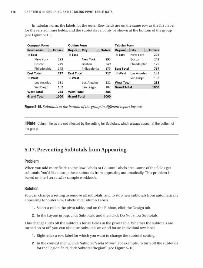
In Tabular Form, the labels for the outer Row fields are on the same row as the first labelfor the related inner fields, and the subtotals can only be shown at the bottom of the group(see Figure 5-15).

Figure 5-15. Subtotals at the bottom of the group in different report layouts

■Note Column fields are not affected by the setting for Subtotals, which always appear at the bottom ofthe group.

5.17. Preventing Subtotals from Appearing

ProblemWhen you add more fields to the Row Labels or Column Labels area, some of the fields getsubtotals. You’d like to stop these subtotals from appearing automatically. This problem isbased on the Stores.xlsx sample workbook.

SolutionYou can change a setting to remove all subtotals, and to stop new subtotals from automaticallyappearing for outer Row Labels and Column Labels.


2. In the Layout group, click Subtotals, and then click Do Not Show Subtotals.

This change turns off the subtotals for all fields in the pivot table. Whether the subtotals areturned on or off, you can also turn subtotals on or off for an individual row label.

1. Right-click a row label for which you want to change the subtotal setting.

2. In the context menu, click Subtotal “Field Name”. For example, to turn off the subtotalsfor the Region field, click Subtotal “Region” (see Figure 5-16).


Figure 5-16. Turn Subtotal on or off for an individual row label.

Using this command toggles the Subtotal setting—if the Subtotal setting was on, it isturned off. The subtotal for the selected field appears in the position that was last specified forthe pivot table. For example, if subtotals were at the top of the group, and then you turned offsubtotals, the field’s subtotals appear at the top of its group.

5.18. Creating Multiple Subtotals

ProblemRegion and City fields are in the Row Labels area in your pivot table. Two fields are in the Val-ues area: Sum of Quantity (Qty) shows the total quantity for each city, and Count of OrderDateis displayed with the heading Orders. A subtotal row exists for each region, which shows thetotal quantity and total order count for each region. You’d like another row of subtotals foreach region, to show the average quantity and order count. This problem is based on theSubtotalsMulti.xlsx sample workbook.

SolutionYou can change the field settings for the Region field and it will show more subtotal rows:

1. Right-click one of the Region row labels, and in the context menu, click Field Settings.

2. In the Field Settings dialog box, click the Subtotals & Filters tab, and then in the Subto-tals section, click Custom.

■Note When you select Custom, the Automatic subtotal is removed.

3. In the list of functions, click each function you want to use as a subtotal, and then clickOK. In this example, click Sum and Average.

4. Format the subtotal values with the number of decimal places you prefer.

■Note When you select multiple Custom subtotals, the subtotals are displayed at the bottom of the group,even if you set the option to show subtotals at the top of the group.


How It WorksWhen multiple fields are in the Row Labels area or the Column Labels area, the last field in thelist is the inner field, and all the other fields are outer fields. In the pivot table, each outer fieldautomatically displays subtotals, unless you turned off that feature.

By default, the subtotals are set as Automatic, and they use the same summary functionas each field in the Values area (see Figure 5-17, in the table at the left).

Figure 5-17. Automatic Subtotals (left) and Custom Subtotals (right)

When you use Custom subtotals, all fields in the Values area use the same custom subto-tal function (see Figure 5-17, the table at the right). This is not a problem if all the Value fieldsuse the Sum function, but if other summary functions are used, the results may not be satis-factory. For example, in the example show at the right in Figure 5-17, the OrderDate field wasused to create a count of records. The count looks correct for each city, but the subtotal rowsuse the date’s numeric value, and the sum and average are based on those numbers, not onthe count of records.

If you use Custom Subtotals, be cautious if you’re using summary functions other thanSum in the Values fields.

5.19. Showing Subtotals for Inner Row Labels

ProblemIn your pivot table, Region and City are in the Row Labels area. You created custom subtotalsfor the Region field, to show the Sum and the Count. You want to show Sum and Count subto-tals for the City field, too, but subtotals aren’t showing for the City field. This problem is basedon the SubtotalsInner.xlsx sample workbook.

SolutionWhen added to the pivot table, the innermost fields in the Row Labels and Column Labelsareas don’t automatically display subtotals. You can format them to show subtotals.


1. Right-click one of the row labels for the City field, and in the context menu, click FieldSettings.

2. On the Subtotals & filters tab, in the Subtotals section, select Custom.

3. In the list of functions, click each function you want to use as a subtotal, and then clickOK. In the sample file, click the Sum and Count functions.

■Note All the subtotals for the innermost field appear after the last item, listed in the sort order for theinnermost field.

5.20. Simulating an Additional Grand Total

ProblemIn your pivot table, Category is in the Row Labels area, Region is in the Column Labels area,and Quantity is in the Values area, as Sum of Quantity. The Grand Total shows the Sum ofQuantity, and you’d like to show another Grand Total, with the Average of Quantity for eachRegion. When you try to change the summary function for the Grand Total, it changes thefunction for all the Values. This problem is based on the GrandAdd.xlsx sample workbook.

WorkaroundYou can’t change the summary function for the Grand Total row or column. To simulate anadditional grand total, you could use one of the following techniques:

• Add another copy of the Quantity field to the Values area, and set its summary functionto Average.

• Create a copy of the pivot table, and remove the Category field from the Row Labelsarea, to show just the heading rows and grand total. Then, change the grand total, so itsummarizes by Average (see Figure 5-18).

Figure 5-18. A copy of the pivot table shows heading and grand total only.

• If you don’t want another field in the Values area, and you just want the average at thebottom of the pivot table, you can use the following technique:

a. Add a new column in the source data with the heading Avg.

b. In the new column, enter the same value for all record, such as a 1 or a space char-acter, or leave all the cells blank.


c. Refresh the pivot table, and then add the Avg field as the first field in the RowLabels area.

d. You can type a new caption for the Avg field’s item. For example, if you left the cellsin the source data blank, replace the (blank) caption with a space character, or AllCategories.

e. Right-click the Avg row label, and in the context menu, click Field Settings.

f. In the Field Settings dialog box, select the Subtotals & Filters tab.

g. In the Subtotals section, select Custom, select the Average function, and then clickOK.

h. On the Ribbon, click the Design tab.

i. In the Layout group, click Subtotals, and then click Show All Subtotals at Bottom ofGroup.

The pivot table shows each Region’s average quantity just above the Grand Total row (seeFigure 5-19).

Figure 5-19. Region Averages created with a special subtotal

5.21. Hiding Specific Grand Totals

ProblemIn the Values area of your pivot table, you have Sum of Quantity and Quantity as % of Row.You’d like to hide the Grand Total for % of Row, because every row is 100%. You don’t want toremove the grand total for Sum of Quantity. This problem is based on the GrandHide.xlsxsample workbook.

WorkaroundYou can’t hide specific grand totals within the pivot table. However, you could use one of thefollowing workarounds:

• Manually hide the worksheet column that contains the % of Row totals.

• Change the font and fill color to white for the % of Row grand total. The columnappears empty, and the results stay hidden, even if you change the pivot table layout.


5.22. Totaling Hours in a Time Field

ProblemIn your source data, you record the hours you worked on different projects. In the pivot table,you want the total hours per project, but the results are shown as time rather than total hours.For example, you worked for 25 hours on Project C: 10 hours+10 hours+5 hours. However, inthe pivot table the sum of 10:00+10:00+5:00 is shown as 1:00 A.M. instead of 25:00 hours. Thisproblem is based on the TotalHours.xlsx sample workbook.

SolutionIn the pivot table, format the cells that contain total times with the number format [h]:mm:ss,and they’ll total correctly. To apply this format, do the following:

1. Right-click a value cell in the TimeSpent field.

2. Click Number Format.

3. In the Format Cells dialog box, in the Category list, click Time.

4. In the Type list, click 37:30:55, and then click OK.

■Note With some regional settings, the 37:30:55 time format is not listed. You can create a custom format[h]:mm:ss;@. This time format totals the hours, instead of calculating the time from the hours.

5.23. Displaying Hundredths of Seconds

ProblemIn your source data there are times, with a custom format of m:ss.00. The times show correctlyin the worksheet—for example, 5:15.25—but they are rounded in the pivot table, with all thehundredths showing as zero—for example, 5:15.00. This problem is based on theTime100th.xlsx sample workbook.

WorkaroundTo correctly display the times in the pivot table, you can use the following workaround:

1. In the source data, add a column, TimeCalc, with a formula that refers to the time col-umn—for example, =B2.

2. Format this column as General instead of Time.

3. Add the TimeCalc field to the pivot table, replacing the original time field, and format itwith the custom number format of m:ss.00.


Modifying a Pivot Table

In this chapter, you’ll find solutions for problems you encounter as you make changes to yourpivot tables. One of the greatest benefits of using pivot tables is this: after you create a pivottable, you can easily modify it. You can move the fields to a different area of the pivot table,add or remove fields, show or hide items, and make other changes to the layout.

You may encounter problems as you change the layout, with fields that don’t behave asexpected, or features that are unavailable after you move a field. You may want to alter thelabels or values in the pivot table, and have unexpected results when you try to make thechanges. Except where noted, the problems in this chapter are based on the Sales_06.xlsxsample workbook.

6.1. Using Report Filters: Shifting Up When AddingReport Filters

ProblemIn cell A1, above your pivot table’s Report Filter, you entered heading text for the worksheet. Inthe PivotTable Field List, you dragged another field to the Report Filters area, below the exist-ing Report Filter. When you release the mouse button, you get a warning about replacing thecontents of the destination cells (see Figure 6-1). If you click OK, the Report Filters move upand remove the heading in cell A1.

You’d prefer the Report Filters move down when they’re added, so they don’t delete theworksheet heading you created. This problem is based on the RptFilters.xlsx sampleworkbook.

Figure 6-1. Adding a Report Filter deletes text in cells above the pivot table.

123

C H A P T E R 6

WorkaroundWhen you add fields to the Report Filters area, Excel tries to keep the main section of the pivottable in its current position. Existing Report Filters are pushed up to prevent the main sectionfrom moving down. There isn’t a setting you can change to prevent this, but one of the follow-ing workarounds may help:

• Instead of arranging the Report Filters vertically, change them to a horizontal layout, asdescribed in the following section.

• If you have headings on the worksheet, above the pivot table, leave a few blank rowsbetween them and the pivot table. If necessary, insert blank rows before adding fieldsto the Report Filters area.

• If the heading information is only required for printing, move the heading text to theHeader, where it won’t be affected by changes to the pivot table layout. To insert aHeader, on the Ribbon, click the Insert tab, and then click Header & Footer in the Textgroup.

6.2. Using Report Filters: Arranging Fields Horizontally

ProblemYou have added several fields to the Report Filters area, and they’re pushing the pivot tabledown on the worksheet. You’d like to arrange the report filters horizontally, but when youselect a report filter cell on the worksheet, and drag it to the right, you get a lengthy messagethat says you cannot move a part of a PivotTable report. This problem is based on theHorizontal.xlsx sample workbook.

SolutionBy default, the Report Filters are arranged vertically above the body of the pivot table. You canarrange the Report Filters horizontally by changing the PivotTable Options:


2. On the Layout & Format tab, click the arrow in the drop-down list beside Display Fieldsin Report Filter Area, and then click Over, Then Down (see Figure 6-2).

Figure 6-2. Set the Layout options for report filters.

3. Because you selected Over, Then Down, the following drop-down list is labeled “ReportFilter Fields per Row.” Select three as the number of report filters you want across eachrow, before the next row of report filters starts.


CHAPTER 6 ■ MODIFYING A PIVOT TABLE124

How It WorksIf your pivot table has many report filters, you can arrange the filters to make the most effi-cient use of the worksheet space. The report filters should be easily accessible, not spread outtoo far across the worksheet. Avoid a long column of filters above the pivot table, pushing thepivot table body far down the worksheet.

By using the Display Fields in Report Filter Area option, you can find the best balance ofheight and width for the report filter layout. The report filters can be arranged in a single col-umn, a single row, columns of a set number of filters, or rows of a set number of filters. Forcolumn arrangements, use the Down, Then Over option, and for row arrangements, use theOver, Then Down option.

Down, Then Over

When a pivot table is created, the Down, Then Over option is selected by default, and theReport Filter Fields per Column setting is zero. With these settings, the report filters are dis-played vertically, in a single column, with no limit to the number of filters in the column.The zero acts as a “No Limit” setting.

To limit the number of report filters in each column, change the setting from zero toanother number. For example, if you select 2, the report filters are limited to two per column(see Figure 6-3). Once the column limit is reached, the filters move over, to start a new column.

Figure 6-3. Report filters arranged Down, Then Over, two per column

Over, Then Down

If you select the Over, Then Down option, the report filters are arranged in a row. In theReport Filter Fields per Row option, select the number of report filters you want across eachrow, before the next row of report filters starts. For example, if you select two, the report fil-ters are limited to two per row (see Figure 6-4). Once the row limit is reached, the filters movedown, to start a new row.

■Note If the Report Filter Fields per Row option is set at zero, the filters are arranged in a single row.

Figure 6-4. Report filters arranged Over, Then Down, two per row

CHAPTER 6 ■ MODIFYING A PIVOT TABLE 125

6.3. Using Values Fields: Changing Content in the Values Area

ProblemYou use a pivot table to keep track of product samples from each category that were sent toeach sales region. You’d like to enter the sample quantities in the Values area of the pivot table,instead of creating records in the source data. When you try to type in a cell in the Values area,you see the error message “Cannot change this part of a PivotTable report.”

In the pivot table, the Region field is in the Row Labels area, Category is in the ColumnLabels area, and Quantity is in the Values area. This problem is based on theChangeValues.xlsx sample workbook.

WorkaroundYou can’t type in cells in the Values area, with the exception of cells that contain calculateditems. For this example, you could create a calculated item with the name Samples, and aformula of =0. Follow these steps to create a calculated item in the Category field:

1. Select one of the label cells for the Category field. If you don’t select one of these cells,you won’t be able to create the calculated item.

2. On the Ribbon’s Options tab, in the Tools group, click Formulas, and then click Calcu-lated Item.

3. Type Sample as the name for the calculated item.

4. Leave the default formula of =0, and then click OK.

In the pivot table, select one of the calculated item cells and type the number of samplesyou sent to that region (see Figure 6-5).

Figure 6-5. Type a number in a calculated item’s cell.

■Caution If you clear a calculated item’s cell, you won’t be able to make any further changes to that cell.Type a zero instead of pressing the Delete key, and you will be able to edit the cell again later.

For other cells in the Values area, unless the PivotTable settings are changed programmat-ically, you can’t make any changes to the PivotTable values. Even if you programmaticallychange a setting to allow edits to the pivot table values, the original values are restored whenthe pivot table is changed or refreshed.


6.4. Using Values Fields: Renaming Fields

ProblemWhen you add the Quantity field to the pivot table Values area, it’s automatically given the cus-tom name Sum of Quantity. You’d like to change the custom name to Quantity, so it’s easier toread and makes the column narrower. When you select the cell and type Quantity, you get anerror message: “PivotTable field name already exists.” This problem is based on theRename.xlsx sample workbook.

SolutionIf you try to create a custom name that’s the same as a field name in the source data, you seethe error message “PivotTable field name already exists.” In this example, because one of thefields in the source data is named Quantity, you can’t use Quantity as a custom name in thepivot table.

However, you can avoid this problem, by adding a space character to the end of the cus-tom name (see Figure 6-6), and it will be accepted.

Figure 6-6. Add a space character at the end of a custom name.

■Tip Adding a space character is a subtle change to the custom name, and would not be noticed by mostusers. To help those who’ll maintain the pivot table after you’re promoted, create an Admin_Notes sheet inthe workbook. There, you can document custom name changes, calculated items, calculated fields, andother helpful details.

6.5. Using Values Fields: Arranging Vertically

ProblemYou added two fields to the Values area, and the Values fields are listed horizontally with theColumn Labels fields. You want the Values fields arranged vertically, under the Row Labels.This will make the report narrower, and you’ll be able to print it vertically on the page. Thisproblem is based on the Values.xlsx sample workbook.


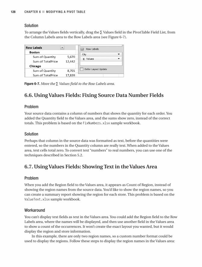
SolutionTo arrange the Values fields vertically, drag the ∑Values field in the PivotTable Field List, fromthe Column Labels area to the Row Labels area (see Figure 6-7).

Figure 6-7. Move the ∑Values field to the Row Labels area.

6.6. Using Values Fields: Fixing Source Data Number Fields

ProblemYour source data contains a column of numbers that shows the quantity for each order. Youadded the Quantity field to the Values area, and the sums show zero, instead of the correcttotals. This problem is based on the FixNumbers.xlsx sample workbook.

SolutionPerhaps that column in the source data was formatted as text, before the quantities wereentered, so the numbers in the Quantity column are really text. When added to the Valuesarea, text cells total zero. To convert text “numbers” to real numbers, you can use one of thetechniques described in Section 5.2.

6.7. Using Values Fields: Showing Text in the Values Area

ProblemWhen you add the Region field to the Values area, it appears as Count of Region, instead ofshowing the region names from the source data. You’d like to show the region names, so youcan create a summary report showing the region for each store. This problem is based on theValueText.xlsx sample workbook.

WorkaroundYou can’t display text fields as text in the Values area. You could add the Region field to the RowLabels area, where the names will be displayed, and then use another field in the Values areato show a count of the occurrences. It won’t create the exact layout you wanted, but it woulddisplay the region and store information.

In this example, there are only two region names, so a custom number format could beused to display the regions. Follow these steps to display the region names in the Values area:


1. In the source data, add a new column with the heading RegNum. Enter a region num-ber of 1 or 2 in this column—1 for East region orders and 2 for North region orders.

2. Refresh the pivot table, and add the RegNum field to the Values area, and then summa-rize by Max.

3. To apply a custom number format to display the region names, right-click a cell in theValues area in the pivot table, and in the context menu, click Number Format.

4. In the Category list, select the Custom category.

5. In the Type box, enter [=1]"East";[=2]"North";General.

6. Click OK.

NotesYou can also display a limited amount of text in the Values area by setting the pivot table’soptions to show text instead of empty cells:


2. On the Layout & Format tab, add a check mark to the For Empty Cells Show option,and in the text box, type N/A (see Figure 6-8), and then click OK.

Figure 6-8. Specifying text to display in empty cells

6.8. Using Pivot Fields: Adding Comments to Pivot Table Cells

ProblemYou’d like to add comments to some of the pivot table cells, so users understand what thefields mean, or to explain why certain values are so low. When you add the comments, theydon’t display when you point to the cell in the pivot table. This problem is based on theNoteLink.xlsx sample workbook.

WorkaroundYou can add comments to cells in the pivot table, but the comments are attached to theworksheet cell, rather than to the pivot item’s cell. If you change the pivot table layout, thecomments won’t move with the item, and they may create confusion for users instead ofhelping them.

As another deterrent to using comments in the pivot table, if contextual tooltips areenabled for the pivot table, the tooltips, instead of the comment, appear when a user points toa pivot table cell. If you decide to add comments, you need to turn off the tooltips, and depriveusers of that feature. To turn off the tooltips, follow these steps:



2. In the PivotTable Options dialog box, on the Display tab, remove the check mark fromShow Contextual Tooltips (see Figure 6-9), and then click OK. Users can now see thecomment when they point to a cell, but they can no longer see the contextual tooltipsthat show information about the pivot table.

Figure 6-9. Turning off the Show Contextual Tooltips option

Instead of inserting comments in the pivot table, you could add a column to the sourcedata, and enter brief comments there. A user who has a question about the data in the pivottable could use the Show Details feature to extract the source data and read any notes entered.

Another way to add documentation or comments to the pivot table would be to insert anew worksheet with the name Notes. To help users navigate between the pivot table work-sheet and the Notes sheet, add a hyperlink in a frozen section at the top of each sheet. Followthese instructions to create the links:

1. On the pivot table’s worksheet, in cell D1, type Notes.

2. Select cell D1, and on the Ribbon’s Insert tab, in the Links group, click Hyperlink.

3. In the Link To list at the left, click Place in This Document.

4. In the list of places in the document, click Notes, and then click OK. This creates ahyperlink to cell A1 in the Notes sheet.

5. Click the hyperlink in cell D1, and the Notes sheet is then activated, with cell A1selected.

6. Add a link in Row 1 on the Notes sheet, to return to the pivot table worksheet.

7. To freeze the top row, on the Ribbon’s View tab, in the Window group, click FreezePanes, and then click Freeze Top Row.

6.9. Using Pivot Fields: Collapsing Row Labels

ProblemIn your pivot table, Region, Category, and Store fields are in the Row Labels area. If you col-lapse the East region, the North region is not affected. However, when you collapse the Barscategory in the East region, the Bars category in both regions is collapsed (see Figure 6-10).You only want to collapse Bars in the East region. This problem is based on the Collapse.xlsxsample workbook.


Figure 6-10. Collapsing Row Labels

WorkaroundCollapse and Expand affect all occurrences of a Row Label. Because there’s only one instanceof the East region, in the outermost field, it is the only item that’s collapsed. However, there aremultiple instances of the Bars category, and they all are collapsed. You can’t change this fea-ture to expand or collapse the selected Row Label only.

As a temporary workaround, you could manually hide the worksheet rows that containthe items.

6.10. Using Pivot Fields: Collapsing All Items in theSelected Field

ProblemIn your pivot table, Region, Category, and Store fields are in the Row Labels area. To hide thedetails for a Region or Category item, you can click the Collapse/Expand indicator, at the leftof the region or category label. Occasionally, you want to see the region totals only, withoutthe category and store detail, and you’d like to collapse all the regions at once, instead of col-lapsing each region individually. This problem is based on the Collapse.xlsx sampleworkbook.

SolutionInstead of using the Collapse/Expand indicators, use a command on the context menu, asdescribed in the following steps:

1. Right-click a Row Label for one of the Regions.

2. In the context menu, click Expand/Collapse, and then click Collapse Entire Field.


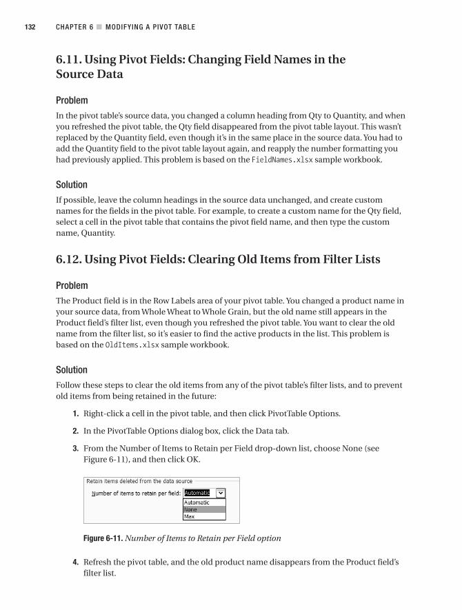
6.11. Using Pivot Fields: Changing Field Names in theSource Data

ProblemIn the pivot table’s source data, you changed a column heading from Qty to Quantity, and whenyou refreshed the pivot table, the Qty field disappeared from the pivot table layout. This wasn’treplaced by the Quantity field, even though it’s in the same place in the source data. You had toadd the Quantity field to the pivot table layout again, and reapply the number formatting youhad previously applied. This problem is based on the FieldNames.xlsx sample workbook.

SolutionIf possible, leave the column headings in the source data unchanged, and create customnames for the fields in the pivot table. For example, to create a custom name for the Qty field,select a cell in the pivot table that contains the pivot field name, and then type the customname, Quantity.

6.12. Using Pivot Fields: Clearing Old Items from Filter Lists

ProblemThe Product field is in the Row Labels area of your pivot table. You changed a product name inyour source data, from Whole Wheat to Whole Grain, but the old name still appears in theProduct field’s filter list, even though you refreshed the pivot table. You want to clear the oldname from the filter list, so it’s easier to find the active products in the list. This problem isbased on the OldItems.xlsx sample workbook.

SolutionFollow these steps to clear the old items from any of the pivot table’s filter lists, and to preventold items from being retained in the future:


2. In the PivotTable Options dialog box, click the Data tab.

3. From the Number of Items to Retain per Field drop-down list, choose None (seeFigure 6-11), and then click OK.

Figure 6-11. Number of Items to Retain per Field option

4. Refresh the pivot table, and the old product name disappears from the Product field’sfilter list.


How It WorksThe default setting in a pivot table is to store deleted items in the pivot table’s pivot cache, aslong as the field is in the pivot table layout. In the Number of Items to Retain per Field, youcan select Automatic, None, or Max from the drop-down list of settings. You can also type aspecific number of items to retain. For example, if you type 2 as the number to retain, the firsttwo old product names would be retained in the filter list. Any additional old names would bedropped from the filter list.

■Note If you remove the field from the pivot table, and refresh the pivot table, the old items are thenremoved, no matter what setting you made for Number of Items to Retain per Field.

6.13. Using Pivot Fields: Changing (Blank) Row andColumn Labels

ProblemIn the source data, a few of the sales orders don’t have a Store number entered. You want blankcells in the Row Labels area and Column Labels area to contain the text “N/A.” In the Pivot-Table Options dialog box, you entered N/A as the text to display in empty cells. However, theempty cells appear as (blank) in the Row and Column Labels areas (see Figure 6-12). Thisproblem is based on the Blanks.xlsx sample workbook.

Figure 6-12. (Blank) items in the Row Labels area

SolutionIn the PivotTable Options dialog box, the setting for empty cells affects cells in the Values area,but not the Row or Column Labels areas. You can manually change the (blank) labels in theRow or Column Labels areas by typing over them in the pivot table. You can type any text toreplace the (blank) entry, but you can’t clear the cell and leave it empty:

1. Select one of the Row or Column Labels that contains the text (blank).

2. Type N/A in the cell, and then press the Enter key.

■Note All other (blank) items in that field will change to display the same text, N/A in this example.


6.14. Using Pivot Items: Showing All Months for Grouped Dates

ProblemIn your pivot table, you added the OrderDate field to the Row Labels area, and grouped thedates by months. To keep the report consistent throughout the year, you want to show all 12month names in your pivot table, even though you only have sales data for the first 3 months.This problem is based on the Months.xlsx sample workbook.

SolutionYou can set the OrderDate field to show all possible items:

1. In the pivot table, right-click one of the OrderDate labels, and then click Field Settings.

2. On the Layout & Print tab, add a check mark to the Show Items With No Data option,and then click OK.

If extra date items, such as <2008-01-01, appear in the Row Labels area, use the OrderDate fil-ter list to hide them.

■Note If the date field is not grouped, no additional dates are displayed in the pivot table, but all dates inthe source data are listed under each subtotal heading.

6.15. Using Pivot Items: Showing All Field Items

ProblemIn your pivot table, the Product and Store fields are in the Row Labels area. Some storeshaven’t ordered every product, but you’d like to see a complete list of stores under each prod-uct. That can make it easier to identify which stores have not ordered one of the products.

A new store has just opened, and you’d also like it included in the list. This problem isbased on the Stores.xlsx sample workbook.

SolutionTo ensure that all the stores appear below each product, you can set the Store field to show allitems:

1. In the pivot table, right-click one of the Store labels, and then click Field Settings.

2. On the Layout & Print tab, add a check mark to the Show Items With No Data option,and then click OK.


However, the new store won’t be included automatically in the list of stores. To have a newstore appear in the pivot table, before any orders are processed, add at least one record to thedata source with the store’s name in the Store field. After real records are added for the store,you can delete the dummy record.

6.16. Using Pivot Items: Hiding Items with No Data

ProblemIn your pivot table, Region and City fields are in the Row Labels area. You created a calculateditem (NewCat) in the Category field, and every City now appears under each Region (seeFigure 6-13). You only want the City names to appear under the region in which they’relocated. This problem is based on the NewCat.xlsx sample workbook.

Figure 6-13. All Cities are listed in each Region, due to the NewCat calculated item.

Workaround When your pivot table includes a calculated item, all the items are listed for fields that inter-sect the calculated item. It’s irritating, it can slow down a large pivot table, and there’s no wayto turn off this behavior. The calculated item generates a Cartesian product, which is a resultwhere every possible combination of items is created in the NewCat calculation.

In the pivot table shown in Figure 6-13, the NewCat value is calculated for each City, foreach Region, and shows a zero result where no data is available.

■Tip If possible, avoid the problem by creating calculations in the source data, instead of using calculateditems in the pivot table.

You can filter the City field, to hide the rows that have a zero in the Grand Total column, asdescribed in the following steps.


1. Right-click a cell that contains a City row label, and in the context menu, click Filter,and then click Value Filters.

2. In the Value Filter dialog box, from the first drop-down list, select Sum of Quantity,which is the Values field you want to check.

3. In the second drop-down list, select Does Not Equal, and in the third box, type 0 (zero),and then click OK (see Figure 6-14).

Figure 6-14. Value Filter dialog box

The rows where the grand total is zero are hidden, and the wayward city names disappearfrom each region.

6.17. Using Pivot Items: Ignoring Trailing Spaces WhenSummarizing Data

ProblemWhen you receive the data for your pivot table, some fields occasionally contain extra spacecharacters at the end of the entry, due to sloppy data entry. In your source data Excel Table,when you apply a filter on the City column, items with differing trailing spaces—such as“Boston” and “Boston ”—show as one entry in the column heading’s filter list. When you addthe City field to the pivot table, “Boston” and “Boston ” show up separately, but you’d like themtreated as one item. This problem is based on the Spaces.xlsx sample workbook.

WorkaroundA pivot table doesn’t ignore trailing spaces, the way an Excel Table’s filter does. You could addanother column to the source table, and use the TRIM worksheet function to remove the extraspaces. For example, do the following if city names are in Column C:

1. Create a new column in the source data, with the heading CityName.

2. In Row 2 of the new column, enter the formula =TRIM(C2).

3. Copy the formula down to the last row of data in the source table. If the source data isstored in an Excel Table, the formula should copy down automatically.

4. Refresh the pivot table, and then add the CityName field to replace the City field in thepivot table.


6.18. Using a Pivot Table: Allowing Drag-and-Drop

ProblemIn previous versions of Excel, you were able to drag fields from the PivotTable Field List ontothe pivot table layout. In Excel 2007, you can only move the fields within the areas in the Pivot-Table Field List. You’d like to move fields onto the worksheet layout, as you did before. Thisproblem is based on the Sales_06.xlsx sample workbook.

SolutionIf you prefer to drag the fields onto the worksheet layout, you can change a pivot table option.


2. Click the Display tab, and add a check mark to Classic PivotTable Layout.

3. Click OK, to close the PivotTable Options dialog box.

4. Point to a field label, such as Region, in the pivot table layout, and when the pointerchanges to a four-headed arrow, drag the field label to a different area (see Figure 6-15). Or, drag fields into the pivot table layout from the PivotTable Field List,or drag field labels out of the pivot table layout.

Figure 6-15. Dragging fields in Classic PivotTable layout

When you enable the Classic PivotTable layout option, the pivot table’s report layoutautomatically changes to Tabular form. You can use this layout, or the Outline form, with theClassic PivotTable layout. If you change the layout to Compact form, the blue outlines of thepivot table areas are still visible on the worksheet when the pivot table is active. However, youwon’t be able to drag-and-drop the fields within the pivot table layout on the worksheet.

6.19. Using a Pivot Table: Deleting the Entire Table

ProblemYou want to remove the pivot table from your workbook, but you can’t delete the entire work-sheet because it contains other data. This problem is based on the Sales_06.xlsx sampleworkbook.


SolutionFollow these instructions, to select the pivot table and delete it:


2. In the Actions group, click Select, and then click Entire PivotTable.

3. On the keyboard, press the Delete key.

This removes the pivot table, and its PivotTable Style formatting, from the worksheet.


Updating a Pivot Table

Most pivot tables are based on source data that continues to change; new records or fieldsmay be added to the source data, existing records are modified, or the source data file ismoved to a new location. You want to ensure that your pivot table contains the latest availabledata and is correctly connected to the source data.

To reproduce the environment in which they were created, sample files must be storedin a C:\_Work folder, for testing. If a different folder is used, the connections will be broken.Create this folder on your computer’s C: drive, and then copy all the sample files to it.Depending on your security settings, you may see a security warning when opening somesample files. To work with the file, you can enable the data connections.

Except where noted, the problems in this chapter are based on the Sales_07.xlsx sampleworkbook.

7.1. Using Source Data: Locating the Source Excel Table

ProblemYou’ve been asked to make changes to the pivot table on the ProductSales worksheet, andyou’d like to find the Excel Table used as its source data. Several Excel Tables are in the work-book, and you aren’t sure which one was used. This problem is based on the Sales07.xlsxsample workbook.

SolutionYou can locate the Excel Table that contains the source data by following these steps:


2. In the Data group, click the upper section of the Change Data Source command.

3. In the Change PivotTable Data Source dialog box, you can see the source table or rangein the Table/Range box. This may be a table name, such as

Sales_East

or a worksheet reference, such as

Sales_East!$A$1:$O$500

139

C H A P T E R 7

4. On the worksheet, you can see the source range, surrounded by a moving border.

5. Click OK, or Cancel, to close the dialog box.

How It WorksIn most cases, the source range is visible, and surrounded by a moving border. If the sourcerange is not activated, it may be on a hidden worksheet. Follow these steps to unhide the sheet:

1. Right-click any worksheet tab, and then click Unhide.

2. In the Unhide Sheet list, select the sheet you want to make visible, and then click OK.

■Tip If the sheet name is not on the list of hidden sheets, it may have been hidden programmatically orremoved from the workbook.

If a range name appears in the Table/Range box and the range is not selected, you cancheck the name definition, to find its location, and to see if there are any problems with thename definition:

1. On the Ribbon, click the Formulas tab, and in the Defined Names group, click NameManager.

2. In the Name Manager, the Excel Tables and defined names are listed (see Figure 7-1).Select a name in the list, and in the Refers To box, you’ll see the worksheet name onwhich the range is located.

Figure 7-1. Name Manager dialog box

CHAPTER 7 ■ UPDATING A PIVOT TABLE140

■Tip If the Refers To formula for a defined name contains #REF! errors, the worksheet, or some of its cells,may have been deleted.

3. If errors are in the formula for a defined name, correct them if possible, or delete theproblem name, and then select a new source for the pivot table.

■Note The formulas for Excel Tables cannot be changed in the Name Manager. Close the Name Manager,and then make the changes on the worksheet where the Excel Table is located. To add rows or columns,drag the resize handle at the bottom right of the last cell in the Excel Table.

7.2. Using Source Data: Automatically Including New Data

ProblemYour pivot table is based on data in the same Excel file, and you frequently add new records tothe source data. Each time you add records, you have to change the source range for the pivottable, to include the new rows.

You would like the source data range to automatically expand to include any new rowsand columns. This problem is based on the NewData.xlsx sample workbook.

SolutionWhen creating a pivot table from Excel data, the best solution is to create a formatted ExcelTable from the data, as described in Section 1.4. Then, use the name of the Excel Table as thesource for the pivot table. The Excel Table automatically adjusts if records are added ordeleted, and the pivot table includes the latest data when it’s refreshed.

If you don’t want to use a formatted Excel Table, you can use a dynamic range as the pivottable’s source. The dynamic range automatically expands to include the new rows andcolumns. Follow these steps to create a dynamic range, in the sample file:

1. On the Orders sheet, select cell A1, which is the top-left cell in the source range.This step isn’t necessary, but it helps you by inserting the cell reference in the namedefinition.

2. On the Ribbon, click the Formulas tab, and then in the Defined Names group, clickDefine Name, to open the New Name dialog box.

3. In the Name box, type a name for the dynamic range, for example, PivotSource.

4. Leave the Scope setting as Workbook, and add a comment (optional), to describe thename or its purpose.

CHAPTER 7 ■ UPDATING A PIVOT TABLE 141

5. In the Refers To box, type an OFFSET formula that references the selected cell

=OFFSET(Orders!$A$1,0,0,COUNTA(Orders!$A:$A),COUNTA(Orders!$1:$1))

or you can use a nonvolatile formula, which may be more efficient in larger work-books, where calculation speed is an issue:

= Orders!$A$1:INDEX(Orders!$1:$10000, COUNTA(Orders!$A:$A),COUNTA(Orders!$1:$1))

The formula is set to a limit of 10,000 rows, which can be increased if required.

6. Click the OK button.

■Caution These formulas do not work correctly if other items are in Row 1 or Column A of the Ordersworksheet. Those items would be included in the count, and would falsely increase the size of the sourcerange, or they could cause an error when the pivot table is refreshed. Blank cells within the data in the rowor column being counted would also cause a problem, reducing the size of the source range. Count a columnand row where there is always a value.

After you create the named range, change the pivot table’s source to the dynamic range:


2. In the Data group, click Change Data Source.

3. In the Table/Range box, type the name of the dynamic range, PivotSource in thisexample, and then click OK.

■Tip While in the Table/Range box, delete the existing table or range. Then, to see a list of defined names,press the F3 key. Click a name in the Paste Name dialog box, to select it, and then click OK.

How It WorksThe OFFSET function returns a range reference of a specific size, offset from the starting rangeby a specified number of rows and columns. The function has three required arguments(shown in bold font), and two optional arguments:

=OFFSET(reference,rows,columns,height,width)

In our example

=OFFSET(Orders!$A$1,0,0,COUNTA(Orders!$A:$A),COUNTA(Orders!$1:$1))


the returned range starts in cell A1 on the worksheet named Orders. It is offset zero rows andzero columns. The height of the range is determined by counting the cells that contain datain Column A of the Orders worksheet:

COUNTA(Orders!$A:$A)

■Note If Column A contains any blank cells within the data range, use a column that does not containblank cells. Blank cells reduce the count and result in a range that is too small.

The width of the range is determined by counting the cells that contain data in Row 1 ofthe Orders worksheet:

COUNTA(Orders!$1:$1)

This creates a dynamic range, because if rows or columns are added, the size of the range inthe defined name increases.

The INDEX formula is similar, but it creates a range that starts in Cell A1 on the Orderssheet, and ends at the cell referenced by the INDEX function.

= Orders!$A$1:INDEX(Orders!$1:$10000,COUNTA(Orders!$A:$A),COUNTA(Orders!$1:$1))

7.3. Using Source Data: Automatically Including New Data in an External Data Range

ProblemIn your workbook, you imported a text file that contains billing data, on to the BillingDataworksheet. This created an external data range that has a connection to the text file. If newbilling records are added to the external file, they appear in the external data range when it’srefreshed. However, the pivot table is based on the imported data, but when you refresh thepivot table, the new records don’t appear.

You can’t create a formatted Excel Table from the external data range, or the connectionto the external data will be lost.

This problem is based on the Billing.xlsx sample workbook. Depending on your secu-rity settings, you may see a security warning when opening the sample file. To work with thefile, you can enable the data connections.

SolutionWhen you import external data to an Excel worksheet, using the commands in the Get Exter-nal Data group on the Data tab of the Ribbon, a named External Data Range is created for theimported data. If you base the pivot table on this named range, it expands automatically asnew records are added, and the pivot table contains all the data.


When you created a pivot table from the external data, you may have used a reference torange of cells, such as BillingData!$A$1:$J$19, instead of using the external data range’s name.If data is added to the external data file, the new data appears in the Excel workbook, when theexternal data range is refreshed. However, the pivot table continues to use the original range,and the new data is not included in the pivot table when it’s refreshed.

Follow these steps to change the pivot table’s data source, so it uses the external datarange name:

1. To see the name of the external data range, right-click a cell in the external data range,and then click Data Range Properties. The range name is shown at the top of the Exter-nal Data Range Properties dialog box. Click OK to close the dialog box.

2. To base the pivot table on this range, select a cell in the pivot table, and then click theOptions tab on the Ribbon.


4. Type the external data range’s sheet name and table name in the Table/Range box. Forexample, if the sheet name is BillingData and the external data range name is Billing_1:

BillingData!Billing_1

5. Click OK.

7.4. Using Source Data: Moving the Source Excel Table

ProblemYour pivot table is based on a named range in another workbook. Using Windows Explorer,you copied the two workbooks to your laptop, so you could work at home, but when you triedto refresh the pivot table, you got an error message: “Cannot open PivotTable source file....”This problem is based on the SalesData.xlsx and SalesPivot.xlsx sample workbooks.

SolutionYou can reconnect the pivot table to the named range, in its new location:

1. Open both files—the file with the pivot table, and the file that contains the source data.

2. Activate the file that contains the pivot table, and then select a cell in the pivot table.

3. On the Ribbon, click the Options tab, and in the Data group, click Change Data Source.

4. While the Change PivotTable Data Source dialog box is open, on the Ribbon, click theView tab. Click Switch Windows, and select the workbook that contains the source data.

5. Select the table that contains the source data, and then click OK.

■Note When you copy the files back to your desktop computer, you’ll have to follow the same steps toreconnect them.


How It WorksWhen you create a pivot table that’s based on data in another workbook, and that workbook isin a different folder, the folder path is stored as part of the source range. When you copy thefiles to a different computer, or move the data source file to a different folder, the pivot tablecan’t connect to it.

To prevent this problem, create and save the pivot table file in the same folder as the datasource file. Then, you can move the two files to any other location, keeping the two files together,and when refreshing, the pivot table looks for the data source file in its current folder.

7.5. Using Source Data: Changing the Source Excel Table

ProblemYour pivot table is based on an Excel Table in the same workbook as the pivot table. Youwant to change the source to a table in another workbook. This problem is based on theCentral.xlsx and East.xlsx sample workbooks.

SolutionFollow these steps to change the source for the pivot table in the Central.xlsx workbook tothe Excel Table in the East.xlsx workbook:

1. Open both workbooks—the file with the pivot table (Central.xlsx), and the file thatcontains the new source data (East.xlsx).

2. Select a cell in the pivot table, and then on the Ribbon, click the Options tab.


4. While the Change PivotTable Data Source is open, on the Ribbon, click the View tab.Click Switch Windows, and then select the workbook that contains the new sourcedata.

5. Select the range for the source data, and the Range reference is created, including theworkbook name, for example:

[East.xlsx]Sales_East!$A$1:$G$21

6. If you select an Excel Table or named range in the other workbook, the name won’t beshown in the Range reference, so you can modify the reference to include it. For exam-ple, if the workbook contains an Excel Table named EastData, you’d type

[East.xlsx]Sales_East!EastData

For a workbook-level range named PivotRange, you’d remove the square brackets and thesheet reference, and then type

East.xlsx!EastData

7. Click OK.


■Note The workbook that contains the source data can be open or closed when you’re using or refreshingthe pivot table. However, if the reference is to an Excel Table, or to a dynamic range in the other workbook,that workbook must be open to refresh the pivot table.

7.6. Using Source Data: Locating the Source Access File

ProblemYou inherited a pivot table that’s based on a Microsoft Access query. When you click theChange Data Source command, you can see the connection name in the Change PivotTableData Source dialog box. However, you can’t see the name of the Access file, or tell which querywas used to create the pivot table. You’d like to find out which database and query were used,so you can make a change to the query. This problem is based on the Shipments.xlsx andShipments.accdb sample files.

SolutionYou can view the connection properties to find the Access file name and path:

1. In the Shipments.xlsx file, select a cell in the pivot table, and then on the Ribbon, clickthe Data tab.

2. In the Connections group, click Properties.

3. In the Connection Properties dialog box, you can see the Connection name at the top.Click the Definition tab.

4. In the Connection File box, you can see the name and path of the database. In theCommand Text box is the name of the Access query.

5. Click Cancel to close the Connection Properties dialog box.

7.7. Using Source Data: Changing the Source Access File

ProblemYou created a pivot table from an Access query, and the Access file was moved to a differentdirectory. When you tried to refresh the pivot table, you got the error message “Could notfind file ‘C:\_Work\Shipments.accdb’.” When you clicked OK, a dialog box appeared with theheading, “Please Enter Microsoft Office Access Database Engine OLE DB Initialization Infor-mation.” Just reading that heading makes you tired, and you’d like to find a simple way toreconnect the pivot table to the database. This problem is based on the Shipments.xlsx andShipments.accdb sample files.


SolutionIf the source database has moved, you can change the connection in the workbook:

1. In the Shipments.xlsx file, select a cell in the pivot table, and on the Ribbon, click Data,and then in the Connections group, click Properties.

2. On the Definition tab, click Browse.

3. In the Select Data Source dialog box, locate and select the database you want to use asthe source, and then click Open.

4. In the Select Table dialog box, select a table or query, and then click OK.

5. Click OK to close the Connection Properties dialog box.

7.8. Using Source Data: Changing the Source CSV File

ProblemYou created a pivot table from a CSV file with the Central region’s data, and you want tochange the source to a different CSV file, that contains the South region’s data.

You tried to change the connection, but the Text Import Wizard opens, instead of con-necting to the new file. You’ve already spent time formatting the pivot table, and you’d rathernot start from scratch.

This problem is based on the PivotCSV.xlsx, South.csv, and Central.csv sample files.

SolutionYou can edit the existing connection, or create a connection to the new CSV file, and then usethat connection for the existing pivot table. To edit the existing connection, you’ll type thepath and the query information. Creating a connection requires more steps, but you canselect the path and query, instead of typing.

Edit the Existing Connection

You can view the connection properties, and then change the information that tells Excelwhere the source file is and which information to use from that source file. Follow these stepsto edit the existing connection:

1. In the PivotCSV.xls file, select a cell in the pivot table.

2. On the Ribbon’s Data tab, in the Connections group, click Properties.

3. Click the Definition tab, where you can see the Connection String and Command Text(see Figure 7-2).


Figure 7-2. Connection string and command text

4. At the beginning of the connection string is the location of the current connection’s fileand the default directory, which you can edit if the new file is in a different folder:

DBQ=C:\_WORK;DefaultDir=C:\_WORK;

5. In the command text, change the file name references to the new file name. For exam-ple, change Central to South. If you want all the fields from the source file, use theasterisk, instead of listing the fields individually:

SELECT South.* FROM South.csv South

6. Click OK, to close the Connection Properties dialog box.

Create a New Connection

The other option is to create a new connection, and use it as the pivot table’s data source.The long list of steps may look daunting, but the entire process should only take a coupleof minutes:

1. Select an empty cell in the workbook that contains the pivot table.

2. On the Ribbon’s Data tab, in the Get External Data group, click From Other Sources,and then click From Microsoft Query. Depending on your security settings, you maysee a security warning.

3. In the Choose Data Source dialog box, on the Databases tab, select <New DataSource>, and then click OK.

4. Name the data source, such as MyCSV_New, and from the drop-down list of drivers,select Microsoft Text Driver (*.txt,*.csv).

5. Click Connect, and leave the check mark for Use Current Directory, because you wantto connect to the South.csv file in the C:\_Work directory.

6. To connect to a file in a different directory, remove the check mark, click Select Direc-tory, select a different directory, and then click OK.

7. Click OK, to close the ODBC Text Setup dialog box.

8. For the default table, select the South.csv file, and then click OK, twice.


9. In the Query Wizard, select the South.csv file as the table, and then click the arrow but-ton to move all its fields into the query.

10. Click Next, three times, to reach the last step in the Query Wizard, and then click Finish.

11. In the Import Data dialog box, select PivotTable Report, and select a location for thistemporary pivot table, and then click OK.

12. Delete the temporary pivot table, which isn’t needed now that the connection is estab-lished.

13. Select a cell in the original pivot table, and on the Ribbon’s Options tab, click ChangeData Source, and then click Choose Connection.

14. Select the new connection, Query from MyCSV_New, in the list, click Open, and thenclick OK.

■Note After you delete the temporary pivot table, you must use the new connection before closing the file,or the connection is automatically deleted.

7.9. Refreshing When a File Opens

ProblemYour pivot table is based on a csv file that is updated every evening, and you want to ensurethe pivot table is updated as soon as the file that contains the pivot table opens. This problemis based on the PivotCSV.xlsx sample file.

SolutionYou can set a pivot table option to refresh the pivot table automatically, as the file opens. Thissetting can be used for pivot tables with an external data source, and for pivot tables based ondata in the same Excel file as the pivot table.


2. On the Data tab, add a check mark to Refresh Data When Opening the File.


7.10. Preventing a Refresh When a File Opens

ProblemIn the Trust Center, you have enabled all data connections, and your pivot table is set torefresh when the file opens. This works well, and ensures that the pivot table is automaticallyupdated each morning, when you open the workbook. However, you occasionally want to


open the file without having the pivot table refresh, so you can review the previous day’s databefore moving forward. This problem is based on the Refresh.xlsx sample workbook.

WorkaroundAlthough you can’t override the Refresh Data When Opening the File setting, you can undo therefresh, after the file has opened, and before you perform any other tasks.

Click the arrow on the Undo button, on the Quick Access Toolbar, and then click to undoany of the listed PivotTable Refresh actions (see Figure 7-3).

Figure 7-3. Undo PivotTable Refresh

■Tip To stop a long refresh in progress, press the Esc key as the file opens.

7.11. Refreshing Every 30 Minutes

ProblemThe database to which your pivot table is connected is updated frequently throughout the day,and you would like the pivot table to refresh automatically every 30 minutes. However, whenyou right-click the pivot table and choose PivotTable Options, you only see an option to RefreshData When Opening the File. This problem is based on the Shipments.xlsx sample workbook.

SolutionThe Refresh Every n Minutes option is in the Connection Properties dialog box. To change thesetting, follow these steps:

1. Select a cell in the pivot table, and then on the Ribbon’s Data tab, in the Connectionsgroup, click Properties.

2. On the Usage tab, add a check mark to Refresh Every 60 Minutes.

3. Change the number of minutes to 30, and then click OK.

■Note This option is only available for pivot tables with an external data source. For pivot tables based onan Excel Table in the same workbook, you can use programming to automatically refresh the pivot tablewhen the source data changes, as described in Chapter 11.


7.12. Refreshing All Pivot Tables in a Workbook

ProblemSeveral pivot tables are in your workbook, based on different Excel Tables. You want to refreshall of them at the same time, instead of refreshing each pivot table individually. This can saveyou several minutes each day, if you don’t have to go to each worksheet and update the pivottables one at a time. This problem is based on the Sales07.xlsx sample workbook.

SolutionTo refresh all the pivot tables in the active workbook at the same time, on the Ribbon’s Data tab,in the Connections group, click the upper section of the Refresh All command (see Figure 7-4).

Figure 7-4. Refresh All command

■Note Using the Refresh All command also refreshes all external data ranges in the active workbook, andit affects both visible and hidden worksheets.

7.13. Stopping a Refresh in Progress

ProblemYou clicked the Refresh button to update your pivot table. The refresh is taking a long time torun, and you want to stop it, so you can work on something else in the workbook, and thenrun the refresh later. This problem is based on the Shipments.xlsx sample workbook.

SolutionTo stop a long refresh, press the Esc key on the keyboard.

If a refresh is running as a background query, you can double-click the Refresh indicatoron the status bar (see Figure 7-5). In the External Data Refresh Status dialog box, click the StopRefresh button, and then close the dialog box.

Figure 7-5. Refresh indicator on the status bar


■Note When you refresh the pivot table, the entire pivot table is affected. You can’t refresh only part of apivot table, or just add the new data to the pivot cache.

7.14. Creating an OLAP-Based Pivot Table Causes Client SafetyOptions Error Message

ProblemWhen you try to create an OLAP-based pivot table, you get the error message “Client Safetyoptions do not allow pass through statements to be issued to the data source.” There is nosample file for this problem, but you may encounter this error as you work with your own files.

SolutionThis error occurs if you have an OLAP cube in which you opted to rebuild the cube every timethe report is opened. To stop the message from appearing when the file opens, you can add anew setting to the Windows Registry.

The steps for this are outlined in the Microsoft Knowledge Base article “You Receive anError When You Create an OLAP Cube-Based PivotTable in Excel,” at http://support.microsoft.com/default.aspx?id=887297.

■Caution If you decide to modify the Windows Registry, as described in the Knowledge Base article,follow the instructions carefully, and observe the warnings to back up the Registry before changing it, aswell as the security cautions.

7.15. Refreshing a Pivot Table on a Protected Sheet

ProblemYou protected the worksheet that contains your pivot table, and under the Allow All Users ofThis Worksheet To list, you added a check mark to Use Pivot Table Reports. However, when youright-click a cell in the pivot table, the Refresh command is disabled, and you can’t refresh thepivot table. This problem is based on the Protect.xlsx sample workbook.

SolutionThe worksheet must be unprotected before you can refresh the pivot table. You can do thismanually or use programming to unprotect the sheet, refresh the pivot table, and then protectthe sheet. A programming example is in Chapter 11.


■Note If pivot tables on different sheets use the same pivot cache, the worksheets for all the related pivottables must be unprotected before any of the pivot tables can be refreshed.

7.16. Refreshing When Two Tables Overlap

ProblemYou have two pivot tables on the same worksheet, and sometimes when you modify one of thepivot tables, you get an error message “A PivotTable report cannot overlap another PivotTablereport.” You want to view them side by side, but would like the second pivot table to move tothe right if necessary, instead of creating the error message. This problem is based on theOverlap.xlsx sample workbook.

WorkaroundIf the pivot table being modified will expand, and if it needs space that’s occupied by the otherpivot table, you’ll see that message. There’s no setting you can change that will move the otherpivot table, to accommodate the first pivot table.

You could store each pivot table on a separate worksheet, and use multiple windows inthe workbook to view them simultaneously:

1. To create a new window in the active workbook, on the Ribbon’s View tab, in theWindow group, click New Window. The title bar shows a number at the end of the filename, to indicate which window is active.

2. To view both windows simultaneously, on the Ribbon’s View tab, in the Window group,click Arrange All.

3. Select Tiled, and add a check mark to Windows of Active Workbook, and then click OK.

4. In each window, activate one of the worksheets that contain a pivot table. With thisarrangement you can see the pivot tables side by side, but they won’t overlap if one ofthe pivot tables is modified.

7.17. Refreshing Pivot Tables After Queries Have Been Executed

ProblemWhen you use the Refresh All command on the Ribbon’s Data tab, your pivot tables arerefreshed before your queries for external data have run. You want to pause the pivot cacherefresh until after the queries are executed, to ensure all the current data is displayed in thepivot table. This problem is based on the Refresh.xlsx sample workbook.


SolutionYou can change a setting for the external data range’s connection:

1. On the Ribbon’s Data tab, click Connections.

2. In the list of connections, select the one you want to change, and then click Properties.

3. On the Usage tab, remove the check mark from Enable Background Refresh, click OK,and then click Close.

With the Enable Background Refresh option off, other processes will wait while Excelrefreshes the query for the external data source.

7.18. Refreshing Pivot Tables: Defer Layout Update

ProblemYou frequently make changes to the pivot table layout, moving several of the fields to a differ-ent area, and then adding and removing fields from the layout. The pivot table updates aftereach change, and this slows things down. You’d prefer to make all the changes, and thenupdate the pivot table. This problem is based on the Sales07.xlsx sample workbook.

SolutionTo prevent the updates from occurring as you make the changes, you can change a setting inthe PivotTable Field List:


2. In the PivotTable Field List, add a check mark to Defer Layout Update.

3. Make the layout changes to the pivot table, and then click Update (see Figure 7-6).

Figure 7-6. Defer Layout Update option and Update button

4. When you finish changing the layout and updating the pivot table, remove the checkmark from Defer Layout Update.

■Note While the Defer Layout Update option is checked, some features of the pivot table, such as RowLabels filters, are disabled.


Pivot Table Security, Limits,and Performance

If other people have access to your pivot table, you may want to disable some of the features,address privacy concerns, monitor access to protected data sources, or prevent users frommaking some changes. Some pivot table security settings require programming, and are dis-cussed in Chapter 11. Other settings can be made manually, and are explained here.

When a pivot table is based on external data, Excel’s security settings can affect your abilityto update the pivot table. You can change the security settings, to control the security warningsdisplayed when you connect to the file. The external data source may have a password you’dlike to store in your Excel file, to make it easier to connect.

Pivot tables can summarize large amounts of data, but a few limits exist to what can gointo different areas of the pivot table layout. When you’re working with very large databases,performance can suffer, and creating or refreshing a pivot table can be extremely slow. Thischapter outlines some of the limits and discusses ways to optimize pivot table performance.

8.1. Security: Storing a Database Password

ProblemYour pivot table is based on a query in an Access database that is password protected, and youwant to use the pivot table without entering the password. Currently, when you open the Excelfile and refresh the pivot table, a Database Password dialog box appears, in which you have toenter the password AjPze$nZ. This password is hard to remember, and there isn’t room at theedge of your monitor for another sticky note. This problem is based on the PivotPwd.xlsxsample file that is connected to a query in the HardwarePwd.accdb database, which is stored ina C:\_Work folder. If a different folder is used, the connections will be broken. Depending onyour security settings, you may see a security warning when opening some sample files. Towork with the file, you can enable the data connections.

SolutionIn the Excel file that contains the pivot table, you can change the connection properties, andstore the password in the connection string:

155

C H A P T E R 8

1. Open the PivotPwd.xlsx file, and refresh the pivot table, entering the password whenprompted.

2. Select a cell in the pivot table, and on the Ribbon, click the Data tab.

3. In the Connections group, click Properties.

4. On the Definition tab, add a check mark to Save Password.

5. In the alert message that appears, you are warned that the password is saved withoutencryption in the Excel file, making your data less secure. To save the password, clickYes. The password is now visible in the connection string (see Figure 8-1).

Figure 8-1. Database password visible in connection string

6. Click OK, to close the Connection Properties dialog box.

■Tip With the database password saved in the connection string, you won’t be prompted for the passwordwhen you open the file and refresh the pivot table. However, the database password is visible in the connec-tion string, so you should store the Excel file in a secure folder on the network.

8.2. Security: Enabling Data Connections

ProblemYou created a workbook with a pivot table connected to an Access database, and when youopen the workbook, you see a security warning in the message bar, above the formula bar (seeFigure 8-2). When you refresh the pivot table, a security notice is displayed, warning thatMicrosoft Office has identified a potential security concern.

Figure 8-2. Security warning in the message bar

You trust the data source, and you would like to work with the pivot table file without see-ing the warnings. This problem is based on the PivotShipment.xlsx sample file that is

CHAPTER 8 ■ PIVOT TABLE SECURITY, L IMITS, AND PERFORMANCE156

connected to a query in the Shipment.accdb database, which is stored in a C:\_Work folder. If adifferent folder is used, the connections will be broken.

SolutionYou can change the data connection settings in Excel’s Trust Center, to hide the message bar,and to allow data connections. These are application level settings, and they affect all work-books you open.

1. Click the Microsoft Office button, and then click Excel Options.

2. Click the Trust Center category, and then click Trust Center Settings.

3. To hide the message bar, click the Message Bar category, and then click Never ShowInformation About Blocked Content.

4. To change the connection settings, click the External Content category.

5. In the Security Settings for Data Connections section, click Enable All Data Connec-tions.

6. Click OK, to close the Trust Center, and then click OK to close Excel Options.

■Note If you prefer not to enable all data connections, you could click Prompt User about Data Connec-tions, in the Security Settings for Data Connections section. Then, refresh the pivot table by using a macrothat runs automatically when the workbook opens, and the warning will not appear. See Chapter 11 forsample code to refresh a pivot table.

8.3. Protection: Preventing Changes to a Pivot Table

ProblemYou want to prevent users from making any changes to the pivot table. They should be ableto view the pivot table, but not change the selected items, type over any of the field names,or rearrange the layout. However, you want users to be able to make changes to data andformulas in other areas of the worksheet. This problem is based on the PivotProtect.xlsxsample file.

SolutionIf you protect the worksheet without enabling pivot table use, users won’t be able to modifythe pivot table.

Preparing the Worksheet

When protecting a worksheet, prepare the sheet first by unlocking cells where changes can bemade. Then, turn on the worksheet protection.

CHAPTER 8 ■ PIVOT TABLE SECURITY, L IMITS, AND PERFORMANCE 157

To prepare the sheet, follow these steps:

1. Select any cells in which users are allowed to make changes. In the sample file, userscan make changes to cell E2.

2. On the Ribbon, click the Home tab.

3. In the Cells group, click Format. The Lock Cell command is enabled if the active cell islocked (see Figure 8-3). To unlock the cells, click Lock Cell.

Figure 8-3. The Lock Cell command is enabled.

Protecting the Worksheet

After you prepare the worksheet, follow these steps to protect the worksheet:

1. On the Ribbon, click the Review tab, and then in the Changes section, click ProtectSheet.

2. If desired, enter a password. If you don’t enter a password, the worksheet will be pro-tected, but it can be unprotected simply by clicking Unprotect Sheet on the Review tabon the Ribbon.

3. Remove the check mark from Use PivotTable Reports, and then check the items youwant enabled on the protected worksheet (see Figure 8-4).

Figure 8-4. Select items to enable on a protected worksheet.

4. Click OK and confirm the password, if one was entered.


How It WorksWhen you protect the worksheet, you can allow or disallow Use PivotTable Reports. Witheither choice, if the worksheet is protected, use of the pivot table is affected.

Not Allowing Use PivotTable Reports

If the worksheet is protected, and Use PivotTable Reports was not selected in the Protect Sheetdialog box, users won’t be able to make any changes to the pivot tables on the worksheet. Forexample, they won’t be able to open the drop-down lists on the pivot field buttons, movefields, remove fields, or add fields. The PivotTable Field List will be hidden.

You can create a pivot chart from a pivot table on the protected sheet, but you won’t beable to change the pivot chart layout or use the PivotChart filter. You can change the pivot chartformatting, chart type, and chart options. If you allow users to Edit Objects on the protectedsheet, a pivot chart can be inserted on the protected sheet. If Edit Objects was not checked, youcan create an empty chart on an unprotected sheet, and change its source to the pivot table.

Other pivot tables, based on the same Excel Table as the pivot tables on a protected sheet,will have some features disabled, such as Refresh.

■Tip If you use worksheet protection to disable the pivot table, many other features of the worksheet arealso disabled, such as AutoSum, Spelling, Subtotals, and Creating or refreshing a pivot table. If these fea-tures are required on the worksheet, you may prefer to use programming to protect the pivot table, whileleaving the worksheet unprotected.

Allowing Use PivotTable Reports

If you enable pivot table use when protecting the worksheet, users can open the drop-downlists on the pivot field buttons, move the fields, remove fields, and add fields. The PivotTableField List can be shown. Users can work with existing pivot tables, but they can’t create a newpivot table on the protected sheet or refresh existing pivot tables.

■Note When enabling PivotTable report use, you can’t control which pivot table features are allowed. If youwant to enable some features, such as selecting items from the Pivot field drop-down lists, and disable otherfeatures, such as changing the layout, you can use programming, as described in Chapter 11.

Even with the Use PivotTable Reports setting turned on, many commands are disabled ifthe worksheet is protected, including the following:

• Report Layout

• Refresh

• Group and Ungroup


• PivotTable Options

• Show Report Filter Pages

• Calculated Field

• Calculated Item

• Enable Selection

• PivotTable Styles

■Tip To refresh the pivot table, the worksheet owner can temporarily unprotect the worksheet, refresh thepivot table, and then protect the sheet.

8.4. Protection: Disabling Show Report Filter Pages

ProblemTo reduce the number of sheets in the workbook, you want to prevent users from using theShow Report Filter Pages feature. Using this feature adds sheets to the workbook, which usersforget to delete, and the workbook size is getting too big. This problem is based on thePivotProtect.xlsx sample file.

SolutionYou can protect the workbook structure, and users won’t be able to add new sheets.

1. On the Ribbon, click the Review tab, and then click Protect Workbook.

2. Add a check mark to Structure, and if desired, enter a password.

3. Click OK to close the dialog box, and if prompted, confirm the password.

With the workbook protected, if users try to use the Show Report Filter Pages feature,they’ll see an error message, “Workbook is protected and cannot be changed.”

You can also use programming to add a prefix to the sheet names as they are created, andthen delete the sheets automatically as the workbook closes. See Chapter 11 for sample code.

8.5. Privacy: Preventing Viewing of Others’ Data

ProblemYour pivot table contains sales data for several departments. You deleted the worksheet thatcontains the source data. Now, you want to send each department a copy of the pivot table withtheir department selected in the Report Filter, and prevent users from seeing data for depart-ments other than their own. This problem is based on the PivotProtect.xlsx sample file.


WorkaroundYou can protect the worksheet without allowing pivot table use, to prevent users from select-ing a different department in the Report Filter. However, users may be able to circumventExcel’s security features, and remove the worksheet protection. Then, they could select a dif-ferent department from the Report Filter, or double-click a cell in the Values area, and use theShow Details feature to re-create the source data.

■Caution Excel worksheet protection can be easily circumvented. If you don’t want users to view theunderlying data, don’t include the data in the pivot table source.

To protect the data, you could create a separate data source for each department and baseits pivot table on that source, with each pivot table in a separate, password-protected work-book. That would provide each department with a fully functioning pivot table, whilemaintaining each department’s privacy.

Or, if users need to see the results, but they do not need to change the pivot table layout,you can create a copy of the pivot table for each department.

1. Select a department name from the report filter.

2. Select the pivot table, right-click a selected cell, and then click Copy.

3. In another workbook, right-click a cell where you would like to create a copy of thepivot table.

4. In the context menu, click Paste Special.

5. Click Values, and then click OK.

6. Format the copied pivot table.

How It WorksIn Excel, you can protect a file with a password when saving it. You can also password-protecta workbook’s structure and windows, as well as its worksheet contents.

Applying Excel security features can help prevent accidental errors or deletions, but maynot thwart a determined malicious attack. A knowledgeable user can circumvent worksheet-and workbook-structure protection by using tools, such as password crackers, that are readilyavailable on the Internet. A strong password on the Excel file, or storing the file in a secure net-work folder can provide better protection.

The “Security Policies and Settings in the 2007 Office System” article provides detailedcoverage of the security settings and privacy options available in Excel, as well as other Officeprograms: http://technet2.microsoft.com/Office/en-us/library/03d787aa-598d-40a9-87ec-31a8ea80e0371033.mspx?pf=true. The “What’s New and What’s Changed” section, on Page 14,outlines the Trust Center, message bar, and documentation-protection features that are in theuser interface in Excel 2007.


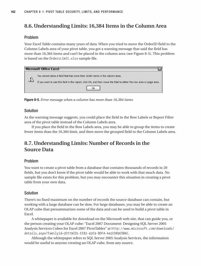
8.6. Understanding Limits: 16,384 Items in the Column Area

ProblemYour Excel Table contains many years of data. When you tried to move the OrderID field to theColumn Labels area of your pivot table, you got a warning message that said the field hasmore than 16,384 items and can’t be placed in the column area (see Figure 8-5). This problemis based on the OrdersLimit.xlsx sample file.

Figure 8-5. Error message when a column has more than 16,384 items

SolutionAs the warning message suggests, you could place the field in the Row Labels or Report Filterarea of the pivot table instead of the Column Labels area.

If you place the field in the Row Labels area, you may be able to group the items to createfewer items than the 16,384 limit, and then move the grouped field to the Column Labels area.

8.7. Understanding Limits: Number of Records in theSource Data

ProblemYou want to create a pivot table from a database that contains thousands of records in 20fields, but you don’t know if the pivot table would be able to work with that much data. Nosample file exists for this problem, but you may encounter this situation in creating a pivottable from your own data.

SolutionThere’s no fixed maximum on the number of records the source database can contain, butworking with a large database can be slow. For large databases, you may be able to create anOLAP cube that presummarizes some of the data and can be used to build a pivot table inExcel.

A whitepaper is available for download on the Microsoft web site, that can guide you, orthe person creating your OLAP cube: “Excel 2007 Document: Designing SQL Server 2005Analysis Services Cubes for Excel 2007 PivotTables” at http://www.microsoft.com/downloads/details.aspx?familyid=2D779CD5-EEB2-43E9-BDFA-641ED89EDB6C.

Although the whitepaper refers to SQL Server 2005 Analysis Services, the informationwould be useful to anyone creating an OLAP cube, from any source.


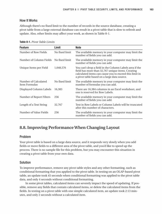
How It WorksAlthough there’s no fixed limit to the number of records in the source database, creating apivot table from a large external database can result in a pivot table that is slow to refresh andupdate. Also, other limits may affect your work, as shown in Table 8-1.

Table 8-1. Pivot Table Limits

Feature Limit Note

Number of Row Fields No fixed limit The available memory in your computer may limit thenumber of fields you can add.

Number of Column Fields No fixed limit The available memory in your computer may limit thenumber of fields you can add.

Unique Items per Field 1,048,576 You can’t drop a field in the Column Labels area if thefield has more than 32,767 unique items. Creatingcalculated items can cause you to exceed this limit ina pivot table based on a large data source.

Number of Calculated No fixed limit The available memory in your computer may limit the Item Formulas number of formulas you can add.

Displayed Column Labels 16,383 There are 16,384 columns in an Excel worksheet, andone is reserved for Row Labels.

Number of Report Filters 256 The available memory in your computer may limit thenumber of fields you can add.

Length of a Text String 32,767 Text in Row Labels or Column Labels will be truncatedafter this number of characters.

Number of Value Fields 256 The available memory in your computer may limit thenumber of fields you can add.

8.8. Improving Performance When Changing Layout

ProblemYour pivot table is based on a large data source, and it responds very slowly when you addfields or move fields to a different area of the pivot table, and you’d like to speed up theprocess. There is no sample file for this problem, but you may encounter this situation increating a pivot table from your own data.

SolutionTo improve performance, remove any pivot table styles and any other formatting, such asconditional formatting that you applied to the pivot table. In testing on an OLAP-based pivottable, an update took 45 seconds when conditional formatting was applied to the pivot tabledata, and only 4 seconds without conditional formatting.

In some pivot tables, calculated items can severely impact the speed of updating. If pos-sible, remove any fields that contain calculated items, or delete the calculated items from thefields. In testing on a pivot table with one simple calculated item, an update took 2:13 min-utes, and only 2 seconds without a calculated item.


If you plan to add or move more than one field, add a check mark to the Defer LayoutUpdate box in the PivotTable Field List (see Figure 8-6).

Figure 8-6. Defer Layout Update option

Then, move or add the fields, and click the Update button, to the right of the Defer LayoutUpdate check box. This reduces the time required, because the fields are all added or moved,and then the pivot table is recalculated once. If this box is not checked, the pivot table is recal-culated after each field is added or moved.

When you finish changing the layout, remove the check mark from the Defer LayoutUpdate check box, to restore full functionality to the pivot table. Some features, such as filter-ing and grouping, are not available when Defer Layout Update is activated.

8.9. Reducing File Size: Excel Data Source

ProblemYour workbook contains a few pivot tables, and it has almost doubled in size, even thoughyou only added a few rows to the Excel Table that’s the pivot table source. Every time you adda pivot table, the size goes up a few megabytes. You’d like to make the file smaller. There is nosample file for this problem, but you may encounter this situation in creating a pivot tablefrom your own data.

SolutionTo reduce the file size, try one of the following options.

Changing the Pivot Table Layout

The pivot table layout can have a dramatic effect on the file size. If the pivot table layout islarge, the used range is larger, and this can increase the file size. If file size is a concern, movemost fields to the Report Filter area before closing the workbook to minimize the used range.

Turn off Save Data with Table Layout

To make the file smaller when saving, you can change a pivot table option so the data isn’tsaved when the workbook is closed:


2. On the Data tab, remove the check mark from Save Source Data With File.



When the data isn’t saved with the layout, the file size is smaller because the pivot cacheisn’t being saved, and it reduces the time required to save the workbook. When you open theworkbook, you have to refresh the pivot table to rebuild the pivot cache when you want to usethe pivot table. This is slower than refreshing a pivot table with a saved cache.

Storing the Excel Table in a Separate Workbook

The Excel Table on which the pivot tables are based can be stored in a separate workbook.This reduces the size of the workbook that contains the pivot tables. The Excel Table workbookcan remain closed when working with the pivot table file, which reduces the amount of mem-ory used.

Save in Excel Workbook Format

If you created the workbook in an older version of Excel, you may be using the workbook inCompatibility mode. Or, if you’re sending the workbook to others who are working in an olderversion of Excel, you may have saved the file in Excel 97–2003 format. Saving the file in thisformat can make the size much larger.

Remove Shapes and Pictures

If any unnecessary shapes or pictures are in the workbook, remove them. These can increasethe file size and slow the performance.

Use an Excel Table As the Source

If your data is stored in Excel, create an Excel Table from the source data, and use that format-ted table as the source. To create the table, select a cell in the source data, and on the Ribbon’sInsert tab, click Insert Table. Some users include many blank rows in the source data range, toensure that new data will be included when the pivot table is refreshed. An Excel Table auto-matically expands to include new data, so you won’t need an artificially big source data range,which could increase the file size.

After creating the table, press Ctrl+End, to go to the last cell in the worksheet’s used range.Delete any unused rows and columns between this cell and the Excel Table.


Printing and ExtractingPivot Table Data

One of the strengths of pivot tables is the capability to change the layout and analyze datafrom different perspectives. Sometimes, though, you want a static picture from the pivot tableand need to print the data. For the most part, pivot tables print the same as other data on aworksheet, but you can apply a few special settings to a pivot table. Some printing issues, suchas printing a copy of the pivot table for each item in the Report Filter field, can be solved byprogramming, and examples are given in Chapter 11.

After you create a pivot table, you may want to extract some of the summarized data foruse in other parts of the workbook. The GetPivotData worksheet function can be used forretrieving specific data from the pivot table. Another way to extract data is to use the ShowDetails feature, which returns records from the source data for the selected pivot table cell.Finally, the Show Report Filter Pages feature can be used to create copies of the pivot table onnewly inserted worksheets.

Except where noted, the RegionSales_09.xlsx workbook is used as the sample file for theproblems in this chapter.

9.1. Repeating Pivot Table Headings

ProblemYour pivot table spans several printed pages and the report filter, row labels, and columnlabels only print on the first page. You want the heading rows and labels on every page, soreaders can understand the report. In your pivot table, the Product and OrderDate fields are inthe Row Labels area, Region is in the Column Labels area, Category is in the Report Filter area,and Sum of TotalPrice is in the Values area. This problem is based on the RegionSales_09.xlsxworkbook.

SolutionYou can set options for the pivot table to make the heading rows and labels appear on everypage when you print the pivot table. There are two settings to change:

167

C H A P T E R 9

• The print titles option determines if the heading rows and columns appear at the topand left on each printed page.

• The row labels option determines if row labels are repeated if their items continue onanother page.

Setting Print Titles

Before you turn on this option, clear any entries for row and column print titles on the work-sheet, as described in the following steps. If either of these boxes contains an entry, the SetPrint Titles option won’t be applied for the pivot table.

1. On the Ribbon, click the Page Layout tab, and in the Page Setup group, click PrintTitles. The Page Setup dialog box opens with the Sheet tab activated.

2. Under Print titles, clear the Rows to Repeat at Top and Columns to Repeat at Leftboxes, and then click OK.


4. On the Printing tab, add a check mark to Set Print Titles, and then click OK.

Repeating Row Labels

You can change a pivot table option so the labels appear on each page. This option has noeffect if the pivot table is in the Compact Form layout, so if one of the other report layouts isn’talready applied, the first step is to select one of them.

■Note This setting will have no effect if the pivot table is in the Tabular Form layout and the option forMerge Labels is turned on.

1. Select a cell in the pivot table, and on the Ribbon’s Design tab, in the Layout group,click Report Layout.

2. Click Show in Outline Form, or click Show in Tabular Form. The pivot table layoutchanges to show each field in the Row Labels area in a separate column, instead of allfields in a single column.


4. On the Printing tab, add a check mark to Repeat Row Labels on Each Printed Page, andthen click OK.

5. Click the Microsoft Office Button, and then point to Print, and click Print Preview, tosee the changes to the report setup. Headings repeat on all pages, and the row labelsrepeat if their items continue on another page. In Figure 9-1, the Banana label isrepeated at the top of Page 2.

CHAPTER 9 ■ PRINTING AND EXTRACTING PIVOT TABLE DATA168

■Note If you zoom in or out in Print Preview, the repeated row labels may disappear temporarily.

Figure 9-1. Headings and row labels repeat in print preview.

How It WorksWhen you turn on the Set Print Titles option, it adds settings to the Print Titles boxes in thePage Setup dialog box, on the Sheet tab. To see the settings, on the Ribbon’s Page Layout tab,in the Page Setup group, click Print Titles.

■Caution If you clear the Print Titles settings in the Page Setup dialog box after turning on the Set PrintTitles option, you have to turn the Set Print Titles option off, and then turn it back on, for it to take effect.

Only one pivot table per worksheet can have the Set Print Titles option selected. If the set-ting is turned on in one pivot table, the option is unavailable in the PivotTable Options dialogbox for other pivot tables (see Figure 9-2).

Figure 9-2. The Set Print Titles option is unavailable.

When the Set Print Titles option is selected, the report filter, row labels, and column labelsprint on every page. If multiple pivot tables are on the worksheet, or other data, the pivot tableheadings also print with those.

CHAPTER 9 ■ PRINTING AND EXTRACTING PIVOT TABLE DATA 169

9.2. Setting the Print Area to Fit the Pivot Table

ProblemYour pivot table frequently changes size, and you have to reset the print area every time youwant to print it. You would like the print area to adjust automatically, so you don’t waste paper,or print only part of the pivot table. This problem is based on the PrintArea.xlsx workbook.

SolutionDon’t set a print area on the sheet with the pivot table, and the entire pivot table will print, nomatter what its size, although it may span several printed pages. To remove an existing printarea, on the Ribbon’s Page Layout tab, in the Page Setup group, click Print Area, and then clickClear Print Area.

If you’re setting a print area because other items are on the sheet that you don’t want toprint, move those items to another sheet, if possible, so you can print the pivot table separately.

If the items must remain on the same sheet as the pivot table, use the following techniqueto quickly set a print area that encompasses the entire pivot table:

1. Select a cell in the pivot table, and on the Ribbon’s Options tab, in the Actions group,click Select, and then click Entire PivotTable.

2. On the Ribbon’s Page Layout tab, in the Page Setup group, click Print Area, and thenclick Set Print Area.

■Tip You can add Select Entire PivotTable and Set Print Area buttons to the Quick Access Toolbar.

9.3. Printing the Pivot Table for Each Report Filter Item

ProblemSeveral stores carry your products, and you were asked to send each store manager a printedcopy of the pivot table, customized to show their sales results. You added the Store field tothe Report Filter area, and you can select a store in the report filter, to show its totals in thepivot table, and then print the worksheet. However, you’d like to find a more efficient way toprint the reports, because you’ll have to do this each week. This problem is based on theRegionSales_09.xlsx workbook.

SolutionYou can use the Show Report Filter Pages feature to create a worksheet for each item in theStore report filter field. Then, you can group the worksheets and print them:


■Tip Before using the Show Report Filter Pages command, select (All) from the Store report filter. If a storeis selected, a worksheet will not be created for that store.

1. Select a cell in the pivot table, and on the Ribbon’s Options tab, in the PivotTable group,click the arrow for Options, and then click Show Report Filter Pages (see Figure 9-3).

Figure 9-3. Show Report Filter Pages command

2. In the Show Report Filter Pages dialog box, select the Store field, and then click OK. Aworksheet with a copy of the pivot table is then created for each store, with the store’sname on the sheet tab, and that store is selected in the report filter.

3. To select all the worksheets created, click the sheet tab for the first store sheet at theleft, and then scroll to see the last store’s sheet tab. Hold the Shift key, and click the laststore’s sheet tab.

■Caution While the sheets are grouped, any changes you make to the active sheet are also made to theother sheets in the group.

4. While the sheets are grouped, you can set the Page Setup options, if desired. On theRibbon’s Page Layout tab, in the Page Setup group, click the commands to set the mar-gins, orientation, or other options. To open the Page Setup dialog box, click the dialoglauncher at the bottom right of the Page Setup group (see Figure 9-4).

Figure 9-4. Page Setup dialog launcher


5. To print the grouped sheets, click the Microsoft Office Button, and then click Print.

6. After printing, you can delete the Store sheets that were created, or close the workbookwithout saving the changes.

9.4. Printing Field Items: Starting Each Item on a New Page

ProblemYour pivot table has Store and Product in the Row Labels area, and when you print your pivottable, you want each store’s data to start on a new page. This enables you to print the entirereport, and send each store its own section. This problem is based on the RegionSales_09.xlsxworkbook.

SolutionYou can change a setting in the Store field, so each item starts on a new page in the printedreport:

1. Right-click one of the Store labels in the pivot table, and then click Field Settings.

2. In the Field Settings dialog box, on the Layout & Print tab, add a check mark to InsertPage Break After Each Item.


■Tip When starting each item on a new page, your pivot table may be easier to understand if you set thepivot table print titles, as described in Section 9.1. This repeats the pivot table headings on each page, sothey’re visible with each store’s data.

NotesUsing the Insert Page Break After Each Item setting won’t ensure all items for a field fit on onepage. It only ensures the next item will start on a new page. For fields with many items, two ormore pages may be required.

If several of the fields have a short list of items, your printed report could end up using anexcessive amount of paper with this setting. You may prefer to turn the setting off and manu-ally adjust the page breaks in Page Break Preview. On the Ribbon’s View tab, in the WorkbookViews group, click Page Break Preview. Dashed lines indicate an automatic page break andsolid lines are manual page breaks. To move a page break, point to it, and drag up or down onthe page.

■Note You can’t move or delete the page breaks created by the Insert Page Break After Each Item setting.


9.5. Printing in Black and White

ProblemYou applied the PivotTable Style Medium 16, which has a blue fill color in the cells, and it hasblack headings with white text. This style is attractive on the worksheet, but it’s difficult to readwhen you print it on your black and white printer. You’d like to print the worksheet without allthe shading, so it’s easy to read and uses less toner or printer ink. This problem is based on theRegionSales_09.xlsx workbook.

SolutionYou can change a page setup option, so the shading is removed when printing:

1. On the Ribbon’s Page Layout tab, click the dialog launcher at the bottom right of thePage Setup group.

2. In the Page Setup dialog box, on the Sheet tab, add a check mark to Black and White.

3. Click OK, to close the dialog box, or click Print Preview, to see the revised coloring. Allthe text is in black font, and all the fill color is removed from the cells.

9.6. Extracting Underlying Data for a Value Cell

ProblemYour pivot table summarizes discount amounts per store, for each category. The Category fieldis in the Column Labels area, Store is in the Row Labels area, and Discount is in the Values area,as Sum of Discount. One store shows a very high discount total for the Cookies category, andyou’d like to see more detail on those orders. None of the other stores is close to this amount,and you wonder if an error occurred in the data, or if there’s another cause for the high amount.This problem is based on the RegionSales_09.xlsx workbook.

SolutionFor pivot tables based on non-OLAP source data, you can use the pivot table’s Show Detailsfeature to extract the source data. For this example, in the pivot table, simply double-click thecell that contains the high discount total.

The Show Details feature extracts the records that contribute to the summarized data, andsends the records to a new sheet in the active workbook. On that sheet, you can examine therecords to see if a problem exists.

■Tip Instead of double-clicking a cell, you can right-click a cell in the Values area of the pivot table, andthen, in the context menu, click Show Details.


If you double-click a cell in the pivot table, you may see an error message that says,“Cannot change this part of a PivotTable report.” The Show Details feature may be turned offin the PivotTable Options dialog box. To turn it on, follow these steps:


2. On the Data tab, add a check mark to Enable Show Details, and then click OK to closethe PivotTable Options dialog box.

How It WorksThe Show Details feature uses the information stored in the pivot table’s pivot cache to createa new sheet that shows the related records from the original source data. It’s a good way toinvestigate anomalies in the summarized data.

The extracted records are copies of the original records in the source data for the pivottable. They are not connected to the original records or to the pivot table.

■Note If you make changes in the exported records, this will have no effect on the pivot table, and thechanges will not be reflected in the original records.

If Show Details is used in a pivot table, all columns from the source data are shown, notjust the fields currently in the pivot table layout.

A new worksheet is automatically created for the extracted records; you can’t change asetting to control where the extracted records are placed.

9.7. Re-creating the Source Data Table

ProblemSomeone accidentally deleted the worksheet that contained the source data for your pivottable, and you would like to re-create it. (Yes, you know you should have kept a backup copy!)This problem is based on the SourceData.xlsx workbook.

SolutionYou may be able to use the pivot table’s Show Details feature to re-create the source data:

1. Ensure that none of the items in the visible fields are hidden. Each report filter fieldshould have (All) selected, and the (Select All) item should be checked in each of therow and column fields. To clear all the filters, on the Ribbon’s Options tab, in theActions group, click Clear, and then click Clear Filters.

■Tip You don’t need to include all fields in the pivot table to see them in the Show Details output. A pivottable with just one field in the Values area, and nothing in the Row Labels, Column Labels, or Report Filterareas, can output all the source data when the grand total cell is double-clicked.


2. On the Ribbon’s Design tab, in the Layout group, click Grand Totals, and then click OnFor Rows and Columns.

3. Double-click the grand total cell at the bottom right of the pivot table.

This should create a new sheet with all the records from the original source data. If thesource table contained formulas, then you have to re-create them, as the Show Details featureexports the data only. If the Show Details feature doesn’t work, check that the Show Detailsfeature is enabled, as described in Section 9.6.

The original records can’t be re-created if the source data was not saved with the file. Thisoption is set in the PivotTable Options dialog box, on the Data tab.

How It WorksThe Show Details feature, where available, creates a new worksheet with the records from thesource data included in the amount shown in the double-clicked cell. The columns are in thesame order as those in the source data, and the list is formatted with the default Table style forthe workbook.

The records exported in the Show Details process are from the current pivot cache. If youhad made changes to the source data, but you hadn’t yet updated the pivot table, thosechanges wouldn’t be reflected in the exported records.

To see the name of the new Excel Table, select a cell in the Excel Table. On the Ribbon’sDesign tab, the Table Name is visible in the Properties group, at the far left. You can changethat name to the same name as the Excel Table that originally held the source data, and thepivot cache may automatically connect to the new source data. If not, you can connect to thenew source range:

1. Select a cell in the pivot table, and on the Ribbon’s Options tab, click Change DataSource. In the Table/Range box, you can see the name of the original source table.

2. Select the new Excel Table, or type the name of the new Excel Table, and then click OK.

■Tip If your pivot table is based on a named range, you may have to redefine the named range if the origi-nal range was deleted.

9.8. Formatting the Extracted Data

ProblemWhen you use the Show Details feature, the underlying data is exported to a table in a newworksheet. You don’t like the blue formatting that’s used on the new table, and you have tospend time formatting each set of records you extract. You’d like the table formatted auto-matically, using a different table style. This problem is based on the RegionSales_09.xlsxworkbook.


SolutionThe extracted records are formatted with the default Table Style for the workbook. To changeto a different default style, follow these steps:

1. Select a cell in one of the Excel Tables in the workbook.

2. On the Ribbon’s Design tab, in the Table Styles group, click the More button, to openthe Table Styles gallery.

3. Right-click a style you like, and then click Set As Default.

Now, when you use the Show Details feature, the extracted records are stored in an ExcelTable that uses the new default table style.

Changing the default table style does not affect the number and date formatting in theextracted records. All the fields in the extracted data use the General number format, or the ShortDate format. There’s no way to control the format of the data exported during a Show Detailsoperation. After the data is exported, you can format the results.

To manually format the data, use the Format Painter button on the Ribbon’s Home tabto copy the formatting from the source Excel Table and apply it to the new table.

9.9. Deleting Sheets Created by Extracted Data

ProblemWhen you use the Show Details feature, data is exported to a new worksheet. This creates extrawork for you, as you have to delete all the created sheets before closing the workbook. You’dlike a quick way to delete the sheets, so they don’t clutter the workbook. This problem is basedon the RegionSales_09.xlsx workbook.

SolutionSave the workbook just before you use the Show Details feature. Then, close the workbookwithout saving the changes, after viewing the additional sheets created by the Show Detailsfeature. Or, save the workbook with a new name to preserve the original workbook without theextra worksheets.

■Note A new worksheet is automatically created for the extracted records; you can’t control where theextracted records are placed.

9.10. Using GetPivotData: Automatically Inserting a Formula

ProblemYou want to refer to a pivot table cell in one of your worksheet formulas, so you can performcalculations using the summarized data. When you type an equal sign, and then click a cell inthe pivot table, Excel inserts a GetPivotData formula:


=GETPIVOTDATA("TotalPrice",$A$3,"Product","Arrowroot")

When you try to copy the formula down the worksheet, the results are the same in every row.You would prefer a simple cell reference, like =B4. This problem is based on the Insert.xlsxworkbook.

SolutionInstead of typing an equal sign, and then clicking a cell in the pivot table, you can type the cellreference yourself. For example, type =B4 instead of clicking Cell B4 to create the reference.

How It WorksThe GetPivotData worksheet function extracts data from the pivot table for a specific pivotfield and pivot item. By default, a GetPivotData formula is automatically created when yourefer to a pivot table cell in a worksheet formula. You can turn this feature on or off.

Although the GetPivotData formula looks complex, and you’re more comfortable usinga simple cell reference, you may get more reliable results by using the GetPivotData function,especially if you plan to add items to the pivot table source.

If you refer to a cell in the pivot table by using a cell reference, the result is whatever iscurrently in that cell. Today, Cell B15 might contain the Grand Total for Sum of TotalPrice but,tomorrow, it may contain the Count of Orders for Cookies in the East Region. If you use aGetPivotData formula, it returns the result from the correct location in the table, as long asthe referenced fields are still in the pivot table. If the referenced fields aren’t visible in thepivot table, then the formula returns an error instead of incorrect data.

■Tip To ensure the referenced fields and items remain visible, you could create a pivot table that is acopy of the main pivot table and stored on a hidden sheet. In your GetPivotData formulas, refer to this hid-den pivot table. Users can change the layout of the main pivot table, and it won’t affect your GetPivotDataformula results.

The GetPivotData function requires two arguments:

=GETPIVOTDATA(data_field,pivot_table)

For example, the formula

=GETPIVOTDATA("TotalPrice",$A$3)

would return the grand total for the TotalPrice values in the pivot table located at Cell A3.

■Tip For non-OLAP-based pivot tables, the data_field argument can be the displayed name, for example,Sum of TotalPrice, or the field name, TotalPrice. For an OLAP-based pivot table, use the name as displayedin the Pivot Field list, for example, Sum of TotalPrice.


Also, you can include up to 126 pairs of pivot fields and pivot items in the GetPivotDatafunction, after the pivot_table argument:

=GETPIVOTDATA("TotalPrice",$A$3,field1,item1,...)

■Tip The field/item pairs can be in any order, following the data_field and pivot_table arguments, but therelated field and item must be listed together, with the field name followed by the item name.

Using the optional field/item pairs enables you to extract specific details from the pivottable. For example, adding one field/item pair, as shown here


would return the total TotalPrice for the Arrowroot product. Product is a pivot field, andArrowroot is an item in the Product field.

Expanding the previous formula with two field/item pairs, as shown here

=GETPIVOTDATA("TotalPrice",$A$3,"Product","Arrowroot","Region","East")

would return the total TotalPrice for the Arrowroot product in the East region. Region is a pivotfield, and East is an item in the Region field.

■Note Because a GetPivotData formula can only display visible data from the pivot table, it’s best suited toa pivot table that has the referenced fields in the Row Labels or Column Labels areas, and limited layoutchanges for the fields used in the GetPivotData formula.

9.11. Using GetPivotData: Turning Off Automatic Insertionof Formulas

ProblemExcel inserts a GetPivotData formula every time you try to link to a cell in the pivot table. Youwant to turn off this feature, so it’s easier to create a simple link to the cells in the pivot table,such as =B4. This problem is based on the Insert.xlsx workbook.

SolutionYou can use a command on the Ribbon to toggle this feature on and off:

1. Select a cell in the pivot table, and then click the Ribbon’s Options tab.

2. In the PivotTable group, click the arrow on the Options command.

3. Click Generate GetPivotData to toggle this feature on and off (see Figure 9-5).


Figure 9-5. The Generate GetPivotData command

9.12. Using GetPivotData: Referencing Pivot Tables inOther Workbooks

ProblemYour GetPivotData formula refers to a pivot table in another workbook. When you open theworkbook and update the links, you get a #REF! error in the GetPivotData formulas. Thisproblem is based on the Linked.xlsx workbook, which has references to the Insert.xlsxworkbook, stored in the C:\_Work folder.

SolutionThe GetPivotData function, like some other Excel functions, only returns data for referencesin the same file, or another open file. To see the results of the GetPivotData formula, open theInsert.xlsx workbook that contains the referenced pivot table.

Or, create the GetPivotData formula in the Insert.xlsx workbook that contains the pivottable, perhaps on a hidden worksheet. Then, in the Linked.xlsx workbook, link to the cell thatcontains the GetPivotData formula in the Insert.xlsx workbook.

9.13. Using GetPivotData: Using Cell References Instead ofText Strings

ProblemYou frequently change the text strings in the GetPivotData formula when you want to see theresults for a different product in your pivot table. It’s time-consuming to modify the formula,and it’s easy to make a mistake as you edit the product names in the formula. This problem isbased on the Reference.xlsx workbook.

SolutionYou can replace the text strings in the GetPivotData formula with references to cells that con-tain the text you want to extract. For example, instead of a formula that contains a productname, like this one,


type the product name in Cell F1, and then change the formula to

=GETPIVOTDATA("TotalPrice",$A$3,"Product",F1)


■Tip Use the Generate GetPivotData feature to create the formula by clicking a cell in the pivot table. Then,in the formula, highlight a text string and its enclosing quotation marks, and click the cell you want to use asa reference for this text.

Type a different product name in the referenced cell, and the formula will show the resultsfor the new name (see Figure 9-6). This is much quicker and easier than adjusting a small partof the formula.

Figure 9-6. Using a cell reference in a GetPivotData formula

■Note The referenced cell should contain only the text, not the double quotes that surround the text inthe formula.

9.14. Using GetPivotData: Using Cell References in anOLAP-Based Pivot Table

ProblemYou want to replace some of the text strings in the GetPivotData formulas that refer to yourOLAP-based pivot table. You’re having trouble getting the syntax right, and the formulas arereturning #REF! errors. This problem is based on the PivotOLAP.xlsx HardwareSales.cub file.

SolutionBecause the OLAP data is in levels, those levels are included in the GetPivotData arguments.When you link to a cell in an OLAP-based pivot table, that starts in Cell A1, the resulting for-mula may look similar to this:

=GETPIVOTDATA("[Measures].[Sum Of Qty]",$A$1,"[Region]","[Region].[All].[West]")


In the sample file, this would return a value of 7010, which is the Sum of Qty for the West region.If you type West in Cell H3, you can replace that part of the formula with a cell reference:

=GETPIVOTDATA("[Measures].[Sum Of Qty]",$A$1,"[Region]","[Region].[All].[" & H3 & "]")

■Note The square brackets in the field and item names mark the start and end of the level names. Whenreplacing text with a cell reference, do not delete the square brackets from the formula, or the formula willreturn an error.

With West in Cell H3, the formula returns the same result, 7010. Type East in Cell H3, and the formula result changes to 10349, which is the Sum of Qty for the East region (see Figure 9-7).

Figure 9-7. Using a cell reference for an OLAP-based pivot table

9.15. Using GetPivotData: Using Cell References for Value Fields

ProblemIn your pivot table, the Quantity and TotalPrice fields are in the Values area, and Product is inthe Row Labels area. When you link to a cell in the pivot table, a GetPivotData formula is auto-matically created, and shows “TotalPrice” as the first argument:


You’d like to make the formula more flexible, so you type TotalPrice in Cell E1, andchange the formula to refer to that cell:

=GETPIVOTDATA(E1,$A$3,"Product","Arrowroot")

The formula returns a #REF! error, even though Cell E1 contains the correctly typed fieldname, “TotalPrice”. This problem is based on the Insert.xlsx workbook.


SolutionTo use a cell reference for the value field, concatenate an empty string at the start or end of thereference. For example, you could use

=GETPIVOTDATA("" & E1,$A$3,"Product","Arrowroot")

or

=GETPIVOTDATA(E1 & "",$A$3,"Product","Arrowroot")

9.16. Using GetPivotData: Extracting Data for Blank Field Items

ProblemIn the source data, some of the orders do not have a store number entered. In the pivot table,the Store field is in the Row Labels area, and a (blank) item is listed. You want to extract thetotal for this item using a GetPivotData formula. This problem is based on theGetPivotData.xlsx workbook.

SolutionIn the formula, leave an empty reference where the item name argument would appear. Forexample, the formula to return the total quantity for store 3000 is

=GETPIVOTDATA("Sum of Quantity",$A$3,"Store","3000")

and for the (blank) store item

=GETPIVOTDATA("Sum of Quantity",$A$3,"Store",)

If you’re using cell references in the formula, the referenced cell should contain the text(blank). For example, if Cell H2 contains (blank), the following formula will return the totalQuantity for the (blank) store item:

=GETPIVOTDATA("Sum of Quantity",$A$3,"Store",H2)

9.17. Using GetPivotData: Preventing Errors for Missing Items

ProblemIn your pivot table, Product is in the Row Labels area, Region is in the Column Labels area, andQuantity is in the Values area. You use a GetPivotData formula to return the total quantity soldfor each product. With the OrderDate field in the Report Filter area, you can select an orderdate and see the quantity sold for the selected date.

Some products may have no sales for the selected date, and they don’t appear when thefilter is applied. If you refer to these products in a GetPivotData formula, this results in #REF!errors being returned. You would like the formula to return a zero, instead of an error. Thisproblem is based on the Missing.xlsx workbook.


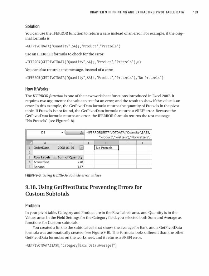
SolutionYou can use the IFERROR function to return a zero instead of an error. For example, if the orig-inal formula is

=GETPIVOTDATA("Quantity",$A$3,"Product","Pretzels")

use an IFERROR formula to check for the error:

=IFERROR(GETPIVOTDATA("Quantity",$A$3,"Product","Pretzels"),0)

You can also return a text message, instead of a zero:

=IFERROR(GETPIVOTDATA("Quantity",$A$3,"Product","Pretzels"),"No Pretzels")

How It WorksThe IFERROR function is one of the new worksheet functions introduced in Excel 2007. Itrequires two arguments: the value to test for an error, and the result to show if the value is anerror. In this example, the GetPivotData formula returns the quantity of Pretzels in the pivottable. If Pretzels is not found, the GetPivotData formula returns a #REF! error. Because theGetPivotData formula returns an error, the IFERROR formula returns the text message,“No Pretzels” (see Figure 9-8).

Figure 9-8. Using IFERROR to hide error values

9.18. Using GetPivotData: Preventing Errors forCustom Subtotals

ProblemIn your pivot table, Category and Product are in the Row Labels area, and Quantity is in theValues area. In the Field Settings for the Category field, you selected both Sum and Average asfunctions for Custom subtotals.

You created a link to the subtotal cell that shows the average for Bars, and a GetPivotDataformula was automatically created (see Figure 9-9). This formula looks different than the otherGetPivotData formulas on the worksheet, and it returns a #REF! error:

=GETPIVOTDATA($A$3,"Category[Bars;Data,Average]")


Figure 9-9. GetPivotData formula for custom subtotal

You’d like to fix the GetPivotData formula so it returns the correct result. This problem isbased on the Subtotals.xlsx workbook.

SolutionWhen linking to custom subtotals at the bottom of a group, the automatically generatedGetPivotData formulas return a #REF! error. This is a bug that has existed in Excel for severalversions, but the formula can be easily corrected.

To fix the formula so it calculates correctly, remove the “Data,” from the formula. Thecorrected formula for this example is

=GETPIVOTDATA($A$3,"Category[Bars;Average]")

How It WorksIf subtotals are shown at the top of the group when the GetPivotData formula is created fora custom subtotal, a normal GetPivotData formula is inserted. If subtotals are at the bottom,a GetPivotData formula with a Data reference is created.

■Note If there are multiple subtotals for a field, the subtotals cannot be shown at the top of the group.

If you move subtotals to the top, after creating a GetPivotData formula with a Data refer-ence, the formula may return incorrect results in some circumstances. Follow these steps tosee an example:

1. Clear the existing pivot table, and create a pivot table layout with Category, Region,and City fields in the Row Labels area, and Quantity in the Values area.

2. On the Ribbon’s Design tab, in the Layout group, click Subtotals, and then click ShowAll Subtotals at Bottom of Group.

3. To create a custom subtotal, right-click a label the Region field, such as East, and thenclick Field Settings.

4. On the Subtotals & Filters tab, click Custom, click Count, and then click OK. In thepivot table, Bars, for the East region, shows a subtotal of 118.


5. Select a cell outside of the pivot table, type an equal sign, and then click the subtotalcell for Bars East. Press the Enter key to complete the formula. The formula in the cellcontains the Data reference and returns a #REF! error:

=GETPIVOTDATA($A$3,"Bars Region[East;Data,Count]")

6. On the Ribbon’s Design tab, change the subtotals to show at the top of the group. Theformula now works correctly, and returns 118 as the result.

7. Remove the City field from the Row Labels area. The GetPivotData formula nowreturns 35314, which is the Sum of Quantity for bars sold in the East, not the count ofbars sold in the East region (see Figure 9-10).

Figure 9-10. GetPivotData formula shows an incorrect result.

If you plan to use the GetPivotData function with custom subtotals, show the subtotals atthe bottom of the group, if possible, or be alert for possible errors.

9.19. Using GetPivotData: Preventing Errors for Date References

ProblemIn your pivot table, OrderDate is in the Row Labels area, and Quantity is in the Values area. Youcreated a GetPivotData formula to extract the total quantity for a specific date. Although thatdate is visible in the pivot table, the formula is returning an error:

=GETPIVOTDATA("Quantity",$A$3,"OrderDate","1/1/08")

This problem is based on the Dates.xlsx workbook.

SolutionIf the date is in the pivot table, but formatted differently, the GetPivotData formula will pro-duce a #REF! error. Instead of entering the date as a text string, you can use either the DATE orDATEVALUE function. For example,

=GETPIVOTDATA("Quantity",$A$3,"OrderDate",DATE(2008,1,1))

or

=GETPIVOTDATA("Quantity",$A$3,"OrderDate",DATEVALUE("1/1/08"))


Both functions return a serial number that represents a date. The arguments of the DATEfunction are Year, Month, and Day. The DATEVALUE function requires a text string as itsargument.

Or, you can enter a valid date in a worksheet cell, and then refer to that cell in theGetPivotData formula:

=GETPIVOTDATA("Quantity",$A$3,"OrderDate",D3)

where Cell D3 contains a valid date, in any format recognized as a date by Excel.

9.20. Using GetPivotData: Referring to a Pivot Table

ProblemTwo pivot tables are on your worksheet, with each one summarizing data for a differentregion. When you create a GetPivotData formula, it includes a reference to a cell in the pivottable as the second argument. In this example, the pivot table is located at Cell A3:

=GETPIVOTDATA("TotalPrice",$A$3)

You’d like to type a cell address on the worksheet, and have the GetPivotData formulareturn the total from the pivot table located at that cell. For example, you want to type H3 inCell E1, and see the total from the pivot table that starts in Column H.

When you refer to Cell E1 in the formula, it returns a #REF! error. This problem is basedon the TwoPivots.xlsx workbook.

SolutionYou can use the INDIRECT function in the GetPivotData function to create a range referencebased on the text in Cell E1. For example:

=GETPIVOTDATA("TotalPrice",INDIRECT(E1))

If you type A3 in Cell E1, the formula returns the total from the first pivot table, and if you typeH3 in Cell E1, the formula returns the total from the second pivot table.

How It WorksThe INDIRECT function requires one argument

=INDIRECT(ref_text)

and returns the range specified by the reference text argument. For example, if Cell E1 con-tains the text A3, the following formula would return the value from Cell A3:

=INDIRECT(E1)


9.21. Creating Customized Pivot Table Copies

ProblemYou’d like to create a separate copy of the pivot table for each store to make it easier for thestore managers to focus on their individual sales results. This problem is based on the Region-Sales_09.xlsx workbook.

SolutionThe Show Report Filter Pages feature creates a copy of the pivot table on a separate worksheetfor each item in the selected report filter field. This is a quick way to create multiple versionsof the pivot table for viewing or printing.

Follow these steps to create the copies:

1. Move the Store field to the pivot table Report Filter area, and then select (All) from itsfilter list.

■Note If an individual item is selected in the filter list, instead of (All), a separate worksheet is not createdfor the selected item.

2. Select a cell in the pivot table, and then click the Ribbon’s Options tab.

3. At the far left, in the PivotTable group, click the arrow for the Options command, andthen click Show Report Filter Pages.

4. In the Show Report Filter Pages window, select the Report Filter field for which youwant to create the pages, and then click OK.

■Tip If a Report Filter field is the active cell on the worksheet, when the Show Report Filter Pages windowopens, that field is selected in the list of Report Filter fields. Otherwise, the first Report Filter field on theworksheet is selected in the list.

How It WorksA copy of the pivot table, on a new worksheet, is created for each item in the field you selectin the Show Report Filter Pages window. In this example, a new sheet is created for each store.The new sheet is named the same as the field item, and that item is selected in the ReportFilter field.


■Note A copy of the pivot table is not created for the (All) item, or the (Multiple Items) selection.

If the pivot table’s options are set to preserve cell formatting on update, and to autofitcolumn widths on update, most formatting from the original pivot table should be retained,including the PivotTable style. Conditional formatting will be lost.

Each copy is based on the original pivot table, and uses the same pivot cache, so this tech-nique may have a minimal impact on the file size, if the layout doesn’t include too many rowsand columns.

Only the pivot table is copied; other data on the same sheet as the original pivot table isnot copied, and neither are page settings, such as footers and margins. If you want to includeother data, such as formulas in cells adjacent to the pivot table, you can create a copy of theworksheet, instead of using the Show Report Filter Pages command.

When the sheets are created, normal sheet name rules are followed.

• The following characters can’t be used in a sheet name:

: \ / ? * [ ]

• If an item name contains one of those characters, a generic name, for example, Sheet5,is used for that item’s sheet.

• The maximum number of characters allowed in a sheet name is 31. Only the first 26characters of the item name are used.

• If a sheet already exists with the item name, or the first 26 characters of the item’s name,a new sheet is created with “(2)” appended to the name.


Pivot Charts

After you create a pivot table, you can create a pivot chart, based on one of the pivot tables inyour workbook. A pivot chart can’t be created on its own; it must be based on a pivot table.Pivot charts are similar to normal Excel charts, but they have some differences and limitations,as described in this chapter. Except where noted, the problems in this chapter are based on theSales10.xlsx sample file.

10.1. Planning and Creating a Pivot Chart

ProblemThe sales manager is preparing for a budget meeting in the East region, and she asked you tocreate a pivot chart, to show the sales for each food category at each store.

You created a pivot table on the Region Pivot worksheet, with Store and Category in theRow Labels area, and Quantity in the Values area. Region is in the Report Filters area, with Eastselected from the drop-down list.

You aren’t sure which type of chart will work best, and you’re having trouble arranging thefields so the chart looks right. The meeting is tomorrow, and you’re running out of time. Thisproblem is based on the Budget.xlsx sample file.

SolutionWhen you create a pivot chart, it will use the same layout as the pivot table on which it’sbased.

• Fields in the pivot table’s Row Labels area become the fields on the pivot chart’scategory axis—the horizontal axis across the bottom of a column or line chart.

• Fields in the pivot table’s Column Labels area become legend fields (series) in the pivotchart—the lines or columns.

• Fields in the pivot table’s Values area become the values in the pivot chart, and theydetermine the height of a column, or the position of the point on a line.

• Fields in the pivot table’s Report Filters area continue to act as filters in a pivot chart.

When planning a pivot chart, consider how you want the fields arranged in the chart. If nofields are in the Column Labels area, the chart will have only one series, representing the fieldsin the Row Labels area. In this example, with Store and Category fields in the Row Labels area,

189

C H A P T E R 1 0

a column chart would have one column for each store’s sales in each category. All the columnswould be the same color.

If you move the Store field to the Column Labels area and create a pivot chart, each storewould be a series, with a different colored column for each store. You could compare the salesof each category, to see which store had the best or worst sales.

If, instead, you move the Category field to the Column Labels area and create a pivotchart, each category would be a series, with a different colored column for each category. Youcould compare the sales at each store, to see which category had the best or worst sales.

In this example, the presentation is to the store managers, who may be interested in howwell their stores are performing, compared to the other stores.

1. In the pivot table, move the Store field to the Column Labels area, and leave theCategory field in the Row Labels area.

2. To create a pivot chart, select a cell in the pivot table, and on the Ribbon, click theOptions tab.

3. In the Tools group, click PivotChart.

4. The Insert Chart dialog box opens, where you can select a chart type and subtype. Forthis chart, select a Column chart type, and a Clustered Column subtype, and then clickOK. A column chart is a good choice if you are comparing sets of numbers, as in thiscase, where you want to compare the total sales for each category at each store.

This creates a pivot chart on the same worksheet as the pivot table (see Figure 10-1). Eachstore is represented by a different color column, with the colors and store numbers shown inthe chart’s legend. The category names appear on the horizontal axis at the bottom of the chart,and you can see which store had the best or worst sales for each category. The height of eachbar represents the quantity sold in each store, for each category. Because the pivot table is fil-tered to show the East region’s sales, the pivot chart is also filtered.

Figure 10-1. The pivot chart shows sales per category.

It may take some experimentation, moving the fields to different areas of the pivot chart,but try to create a chart that presents a limited amount of data, in a clean and simple chartlayout. To see the different layouts available with the Store, Category, and Quantity fields, trythe following:

CHAPTER 10 ■ PIVOT CHARTS190

1. With the pivot chart selected, move Store to the Axis Fields (Categories) area, belowCategory. This creates one series, with the legend entry of Total. All the columns areblue, and two sets of labels are on the horizontal axis. The category names are theouter labels on the axis, and store numbers are the inner labels. This layout lets youcompare the sales for all categories at all stores, but the horizontal axis is crowded,and the single color makes the chart difficult to read at a glance.

2. Move Store above Category in the Axis Fields (Categories) area. This creates one series,with blue columns, and the legend entry of Total. The store numbers are the outerlabels on the horizontal axis, and category names are the inner labels. This layout letsyou compare the sales for all stores and all categories, but the horizontal axis iscrowded, and the labels are hard to read.

3. Move Category to the Legend Fields (Series) area. This creates a different colored seriesfor each category. The store numbers are labels on the horizontal axis, and you cancompare how well the categories sold, within each store.

4. Move Store to the Legend Fields (Series) area, above Category. This creates a differentcolored series for each store’s sales of each category. The legend contains a lengthy listof store and category names, and the chart is crowded and difficult to read.

How It WorksThe Insert Chart Type dialog box shows a list of chart types at the left. At the right are the sub-types available for each chart type. You can point to a subtype and see its name in a tooltip.

Selecting a Chart Type

Unless you changed the setting, the default chart type in Excel is a clustered column chart.Several chart types are available in Excel:

• Column and bar charts are almost the same, except bars are displayed horizontallyacross the chart and columns are vertical. Both of these chart types work well for com-paring specific values, as you’re doing in your chart.

• Line charts and area charts connect the points that represent values and are good forillustrating changes over time. The charts are the same, except the area charts are filledwith color.

• Pie charts and doughnut charts show the percentage each value comprises in the overalltotal. The pie chart type works well when there is a single series and value, such as totalquantity per region. A doughnut chart can show multiple series.

• Surface charts and radar charts are specialized chart types you can use to show differ-ences in the data or aggregated data.

■Note Although they are available in the list of chart types, you cannot use the X Y (Scatter), Bubble, orStock chart types when creating a pivot chart.

CHAPTER 10 ■ PIVOT CHARTS 191

Selecting a Chart Subtype

After you select a chart type in the Insert Chart Type dialog box, its default chart subtype isautomatically selected. You can select a different subtype, to meet the requirements of yourcurrent chart. The following are a few of the options:

• Clustered column and bar subtypes are useful if you want to compare the individualvalues in a series. In the current example, a clustered column lets you compare the cat-egory sales at each store, side-by-side.

• Stacked column and bar subtypes combine individual values in a single column or bar,and they let you compare totals. For example, if you select Stacked Column as the sub-type for the current chart, with Store in the Axis Fields (Categories) area, and Categoryin the Legend Fields (Series) area, the chart will have a single column for each store.Each category is represented by a different color.

• The 100 percent Stacked column and bar subtypes combine individual values in asingle column or bar that represents 100 percent of each item’s value. This lets youcompare percentages within each item. For example, if you select 100 percent StackedColumn as the subtype for the current chart, with Store in the Axis Fields (Categories)area, and Category in the Legend Fields (Series) area, the chart will have a single col-umn for each store. All the columns are the same height, and within each column, eachcategory’s color shows its percentage of the store’s sales.

• Line charts and area charts also have stacked and 100 percent stacked subtypes similarto those for the column and bar charts.

• The remaining chart types have subtypes you can test on your pivot charts. Most ofthese, such as Line with Markers or Exploded Pie, are simply a different format, ratherthan a different layout of the data.

■Tip Avoid using the 3-D chart subtypes, because they distort the representation of the data in your charts.

10.2. Quickly Creating a Pivot Chart

ProblemYou frequently create pivot charts using the clustered column chart type, and you would like aquick way to create one on a chart sheet. You’re tired of navigating through the Ribbon’s tabs,and performing so many steps, just to create a simple chart. This problem is based on theRegions.xlsx sample file.


SolutionYou can press one key on the keyboard, to create a pivot chart on a new chart sheet:


2. On the keyboard, press the F11 key.

A pivot chart is created, on a new chart sheet, in the default chart type and subtype. Youcan format the pivot chart, or change its layout, if required.

How It WorksIf you have not changed the setting, the default chart type is a clustered column chart. If youusually select a different chart type, you can set that type as the default. You can also createyour own chart templates, and set one of those as the default.

Setting the Default Chart Type

Follow these steps to change the default chart type:

1. Select an empty cell on any worksheet.

2. On the Ribbon’s Insert tab, click the dialog launcher at the bottom right of the Chartsgroup.

3. In the Insert Chart dialog box, select the chart type and chart subtype you want to setas the default type. For example, click Line as the chart type, and then click the Linesubtype (see Figure 10-2).

Figure 10-2. Select a chart type and subtype.

■Note The X Y (Scatter), Bubble, and Stock chart types are unavailable when creating a pivot chart. If youselect one of these as the default chart type, you will be unable to create a pivot chart with the F11 shortcut.

4. Click Set as Default Chart, and then click Cancel, to close the dialog box without creat-ing a chart.


Creating a Chart Template

You can create a chart template that stores all the settings you would like to apply to othercharts. For example, if you frequently create a clustered column chart, change the columns togreen, and then add a title and other formatting, you could save a GreenCluster template. Fol-low these steps to create a chart template:

1. Create a chart with the chart type, formatting, and layout you want to save as a tem-plate. The chart can be located on a chart sheet, or on a worksheet.

2. Select the chart, and on the Ribbon’s Design tab, in the Type group, click Save AsTemplate.

3. In the Save Chart Template dialog box, type a file name for the template, such asGreenCluster. The file extension, crtx, is automatically added to the file name when itis saved. Leave the Save In folder unchanged, and your template is saved in the defaultfolder for chart templates.

4. Click Save, to save the template.

To make the template the default chart type, follow these steps:

1. Select an empty cell in the workbook, and on the Ribbon’s Insert tab, click the dialoglauncher at the bottom right of the Charts group.

2. In the list of chart types, click Templates, and then click your template.

3. Click Set As Default Chart, and then click Cancel, to close the dialog box.

4. If you created a chart as a model for the template, you can delete it—click the chart,and then press the Delete key.

10.3. Creating a Normal Chart from Pivot Table Data

ProblemThe sales manager asked you for a pivot chart that shows the number of days customers waitfor service in the East region. You summarized the data from your company’s service workorders, with Wait days in the Row Labels area, District in the Report Filters area, and Count ofWO (work orders) in the Values area.

The best chart type for this would be an X Y (Scatter) chart, because the chart will havenumbers on both axes—the number of wait days and the count of work orders. However,when you try to create the chart, you get an error message that says, “You cannot use an X Y(Scatter), Bubble, or Stock chart type with a chart that has been created from PivotTabledata. Please select a different chart type.” This problem is based on the WaitDays.xlsxsample workbook.

WorkaroundAlthough you can’t create some types of charts from pivot table data, you can link the data toanother worksheet, and then use the linked data as the source for a chart.


1. In the pivot table, select the cells you want to include in the chart. In this example,select cells A4:B21, which contain the wait days and the count of work orders.

2. Right-click one of the selected cells, and then click Copy.

3. Right-click the cell where you would like to paste the linked cells, and then click PasteSpecial. In this example, the data is pasted onto the PivotLink worksheet.

4. In the Paste Special dialog box, click Paste Link. Add headings above the linked data,such as Days and WOs.

5. To create a chart, select a cell in the linked data.

6. On the Ribbon’s Insert tab, click the Scatter command, and then click the first chartsubtype. This creates a scatter chart on the same worksheet as the linked data.

7. Format the chart as desired.

10.4. Filtering the Pivot Chart

ProblemYou created a pivot chart for the sales manager to use at the upcoming budget meeting. Thepivot chart is on its own chart sheet, and when you want to select a different category in theReport Filter, you have to go to the pivot table and make the changes.

You want it to be easy for the sales manager to select a different category or change thechart layout during the meeting, without having to leave the chart sheet. This problem isbased on the Filter.xlsx sample file.

SolutionIf you display the PivotChart Filter pane and the PivotTable Field List pane, you can make thelayout and filter changes while working on the chart. Follow these steps to display thesepanes:

1. Select the pivot chart, and on the Ribbon, click the Analyze tab.

2. In the Show/Hide group, click Field List, to display the PivotTable Field List pane, andthen click PivotChart Filter, to show the PivotChart Filter pane (see Figure 10-3).

Figure 10-3. Field List and PivotChart Filter commands

■Tip Hide the PivotTable Field List pane and the PivotChart Filter pane after you finish modifying the pivotchart. This makes more room to view the chart’s data.


How It WorksThe PivotTable Field List lets you change the pivot chart layout, and the PivotChart Filter panelets you filter the fields in the pivot chart.

Using the PivotTable Field List

The PivotTable Field List can be visible or hidden when a pivot chart is active. Use it to movefields in and out of the chart layout, or to a different area of the pivot chart layout.

When the pivot chart is active, two of the area names change, to match the areas in the chart:

• The Column Labels area changes to the Legend Fields (Series) area.

• The Row Labels area becomes the Axis Fields (Categories) area.

Move fields from one area of the PivotTable Field List to another, or add or remove fieldsfrom the pivot table layout. This changes the chart’s appearance, as well as the pivot table onwhich the pivot chart is based.

Using the PivotChart Filter Pane

The PivotChart Filter pane (see Figure 10-4) enables you to filter the fields in the pivot chart’sReport Filter, Axis Fields (Categories), or Legend Fields (Series) areas. You can also use it tosort the axis fields and legend fields.

Figure 10-4. The PivotChart Filter pane

• At the top right of the PivotChart Filter pane is a button that toggles the PivotTable FieldList from visible to hidden (see Figure 10-4).

• To filter a field, click the arrow in the field’s drop-down list, and then check the itemsyou want to show. These filters work just as they do for the fields in the pivot table. Forthe axis and legend fields, you can also apply Value, Date, and Label filters from the fil-ter drop-down lists.

• To sort the axis or legend fields, click the arrow in the field’s drop-down list, and thenclick one of the sort options.


10.5. Changing the Series Order

ProblemYou created a line chart to show the sales per category over several months. The categories arelisted in the legend, and you would like them sorted alphabetically. This problem is based onthe SalesDate.xlsx sample file.

SolutionWhen you create a pivot chart, the series order is automatically applied, based on the sort set-ting for the field in the pivot table on which the pivot chart is based. To change the sort order,follow these steps:

1. Select the pivot chart, and then display the PivotChart Filter pane.

2. Click the arrow in the drop-down list for the field you want to sort. In this example,click the arrow for the Legend Fields (series), where the Category field is listed.

3. Click Sort A-Z, to sort the categories in ascending order (see Figure 10-5).

Figure 10-5. Sort Options in the PivotChart Filter pane

10.6. Changing Pivot Chart Layout Affects Pivot Table

ProblemWhen you change the pivot chart layout, the related pivot table is also changed. You want thepivot chart and pivot table to work independently. This problem is based on theSalesDate.xlsx sample file.

WorkaroundIf you rearrange the fields in a pivot chart, the same changes are made to the related pivottable. You can create a second pivot table, by copying the first one, and arrange it as you’d like.Then, when you change the pivot chart, only the original pivot table is affected. You can hidethe first pivot table that’s connected to the pivot chart and use the second pivot table for dis-playing or printing.

If you require several charts based on the same pivot table, but with different layouts, cre-ate multiple pivot tables as copies of the original pivot table. Create one pivot chart from eachof the secondary pivot tables, and rearranging one won’t affect the others.


10.7. Changing Number Format in Pivot Table AffectsPivot Chart

ProblemFor the sales manager’s presentation, you’d like the sales amounts on the pivot chart’s axis for-matted as thousands, so the numbers take less room. If you change the number format in thepivot table, the pivot chart’s number format also changes, but you’d like the pivot table toshow the full number. This problem is based on the Numbers.xlsx sample file.

SolutionYou can change a setting in the pivot chart, so the numbers are formatted separately.

1. In the pivot chart, right-click a number in the axis, and then click Format Axis.

2. In the Format Axis dialog box, click Number.

3. Click the Custom category. This automatically removes the check mark from Linked toSource, which disconnects the axis labels from the formatting in the pivot table.

4. In the Format Code box, type a code for the formatting, such as

#,"K";-#,"K"

5. Click Add, to create the custom number format code, and then click Close.

10.8. Formatting the Data Table

ProblemYou spent an hour applying conditional formatting to the data cells in the pivot table, andformatting the numbers as currency. Then you added a data table to the pivot chart, from theRibbon’s Layout tab. The number formatting was displayed correctly, but the conditional for-matting didn’t appear. You’d like to show all the formatting in the data table. This problem isbased on the CondFormat.xlsx sample file.

WorkaroundThe number formatting from the source data will be used in the chart’s data table, but otherformatting won’t be displayed. Instead of displaying a data table, you could place the pivotchart on a worksheet, close to the pivot table, where the formatted data will be visible.

10.9. Including Grand Totals in a Pivot Chart

ProblemThe grand total row is visible in the pivot table, and you want to include the totals in thepivot chart. You can’t find any setting that lets you include them. This problem is based onthe Totals.xlsx sample file.


WorkaroundThe pivot chart is limited to showing the data from the pivot table’s Values area. Other data,such as subtotals, or grand totals or additional series, such as a target line, can’t be added.

You could create a normal chart from the data, as described in Section 10.3, and includethe grand totals in the linked data.

10.10. Converting a Pivot Chart to a Static Chart

ProblemThe sales manager asked you to send each store a copy of the pivot table you created. Beforeyou send them, you want to change the pivot chart to a static chart that isn’t connected to thepivot table. That way, you can send the pivot chart without the underlying detailed data. Thisproblem is based on the Sales10.xlsx sample file.

SolutionTo change a pivot chart to a static chart, you can copy the pivot chart to a different workbook:

1. Right-click the pivot chart’s Chart area, and then in the context menu, click Copy.

2. Activate the workbook into which you want to paste the pivot chart.

3. Right-click the cell where you would like to place the upper-left corner of the chart,and in the context menu, click Paste.

10.11. Showing Field Names on the Pivot Chart

ProblemYou created a pivot chart to show the sales of your low-fat and low-calorie products, and twoof the fields contain Yes/No values. When you add these fields to the pivot chart, the fieldnames aren’t visible, and it’s impossible to tell which fields are represented in the pivot chart.You can see the field names in the PivotChart Report Filter, but that won’t be visible when youprint the chart. You want to display the field names on the pivot chart, so readers can under-stand the data. This problem is based on the YesNo.xlsx sample file.

WorkaroundThere’s no setting you can change that will display the field names in the pivot chart. Todescribe the chart contents, you can add a chart title, and you can add axis titles to clarify theitems on the vertical and horizontal axes. For fields where ambiguity exists, you can add a textbox to the pivot chart, to explain the data that’s displayed.


Adding a Chart Title

Follow these steps to add a chart title:

1. Select the pivot chart, and then on the Ribbon, click the Layout tab.

2. In the Labels group, click Chart Title, and then click Centered Overlay Title or AboveChart.

3. Select the placeholder text in the chart title that was added, and type the text you wantin your title.

Adding Axis Titles

Follow these steps to add an axis title:

1. Select the pivot chart, and then on the Ribbon, click the Layout tab.

2. In the Labels group, click Axis Titles, and then click Primary Horizontal Axis Title or Pri-mary Vertical Axis Title.

3. Click one of the options for the selected axis title.

4. Select the placeholder text in the axis title that was added, and then type the text youwant in the axis title.

Adding a Text Box

Follow these steps to add a text box:

1. Select the pivot chart, and on the Ribbon, click the Layout tab.

2. In the Insert group, click Text Box, and then use the pointer to draw a text box on thepivot chart.

3. In the text box, type the text you want to add to the pivot chart.

Formatting the Titles and Text Boxes

After you add titles or text boxes to the pivot chart, you can format them, using the commandson the Ribbon’s Home tab and the Format tab. Select a title or text box in the chart, and thenuse these commands to change the colors, fonts, and effects.

Creating Dynamic Titles and Text Boxes

To make a title or text box more flexible, you can link it to a worksheet cell. The cell can con-tain text or a formula. For example, if your pivot table has a Report Filter for Region, you couldlink the chart title to the cell that shows the selected region’s name.

Follow these steps to link a chart title to a cell:

1. In the pivot chart, click the chart title to select it.

2. Click in the formula bar, and then type an equal sign.

3. Activate the sheet that contains the pivot table, and then click the cell that contains theregion name.


4. Press the Enter key to complete the link.

5. Select a different region in the PivotChart Filter pane and the chart title will change, toshow the new selection.

■Note If you are linking a text box to a cell, click the border of the text box to select it. The cursor shouldnot be flashing inside the text box.

10.12. Refreshing the Pivot Chart

ProblemYou want to refresh the pivot chart, instead of going to the pivot table and doing the refreshthere. However, when you right-click near the center of the pivot chart, the context menudoesn’t contain a Refresh command. This problem is based on the Sales10.xlsx sample file.

SolutionThe context menus show different commands, based on where the pointer is when you right-click. If you right-click the plot area, you see a short context menu, which has commandsincluding Format Plot Area and Select Data. If you right-click the chart area, which is outsidethe plot area, you see a longer context menu. It includes such commands as Format ChartArea, Assign Macro, and Refresh Data.

To determine where the chart area is, point to part of the pivot chart, and hold the pointerstill. A tooltip shows the name of the chart element (see Figure 10-6).

Figure 10-6. A tooltip shows the name of a chart element.

10.13. Creating Multiple Series for Years

ProblemThe service manager asked for a chart that compares the service data for the past two years.You created a line chart from two years of data, but the chart has a single line, with two yearsof dates on the horizontal axis. You want each year to have a separate line in the chart, so you


can compare the number of work orders for each month (see Figure 10-7). This problem isbased on the Service.xlsx sample file.

Figure 10-7. Compare years with a line chart.

SolutionFollow these steps to group the dates and create a line for each year:

1. In the pivot table, right-click a cell in the date field, and then in the context menu,click Group.

2. In the Grouping dialog box, select Years and Months, and then click OK.

3. In the PivotTable Field List, move the Years field to the Column Labels area.

4. Activate the pivot chart, where the years will each be represented by separate lines.

10.14. Locating the Source Pivot Table

ProblemThe sales manager sent you a workbook that contains multiple pivot charts and pivot tables,and he asked you to make some changes. You aren’t sure which charts are based on whichtables, and you would like to figure it out before you start making changes. This problem isbased on the Source.xlsx sample file.

SolutionYou can use the Ribbon commands to find the pivot table that is the source for a pivot chart.

1. Select a pivot chart, and on the Ribbon, click the Design tab.

2. In the Data group, click Select Data.

3. In the Chart Data Range box, you see a formula that includes the workbook name,sheet name, and range in which the source pivot table is located (see Figure 10-8).Click Cancel to close the dialog box.


Figure 10-8. Find the pivot chart’s source data range.

■Note You can’t change the source table for the pivot chart, but the Select Data Source dialog box canhelp you identify the source table for each pivot chart. If you need to base the pivot chart on a different pivottable, you will have to re-create the pivot chart.

10.15. Creating a Combination Pivot Chart

ProblemYou created a clustered column pivot chart to show the sales per category in each city. You’dlike to change the column for New York to a line, so it stands out from the other cities and actsas a target line. You can’t find any combination chart types, so you aren’t sure how to create theline and column chart you need. This problem is based on the Combo.xlsx sample file.

SolutionAfter you create a pivot chart, you can select a series in the chart and change it to a differentchart type.

1. In the pivot chart, right-click a column in the New York series that you want to change.

2. In the context menu, click Change Series Chart Type.

3. In the Change Chart Type dialog box, click the Line chart type and the chart subtypeyou prefer, and then click OK.

10.16. Moving a Pivot Chart from a Chart Sheet

ProblemWhen you right-click the pivot chart, the Move Chart command isn’t available in the contextmenu. You’d like to use this quick way to move the chart, instead of finding the command onthe Ribbon. This problem is based on the Sales10.xlsx sample file.

SolutionThe context menus show different commands, based on where the pointer is when youright-click. If you right-click the Plot area, you see a short context menu, that has com-mands including Format Plot Area and Select Data. If you right-click the Chart area, which


is outside the Plot area, you see a longer context menu. It includes such commands asFormat Chart Area, Change Chart Type, and Move Chart.

10.17. Removing a Pivot Chart

ProblemYou finished working on the pivot chart, and you would like to remove it from the workbookand create a different pivot chart from the data. This problem is based on the Sales10.xlsxsample file.

SolutionYou can delete a pivot table, to completely remove it from the workbook, or you can clear allthe fields and formatting from the pivot chart layout, and start over.

■Caution Clearing the pivot chart also clears the pivot table on which it is based.

Deleting a Pivot Chart on a Worksheet

If you no longer need a pivot chart that’s on a worksheet, you can delete it.

1. Select the pivot chart.

2. On the keyboard, press the Delete key.

Deleting a Pivot Chart on a Chart Sheet

If you no longer need a pivot chart that’s on a chart sheet, you can delete it.

1. Right-click the sheet tab for the chart sheet, and then click Delete.

2. In the confirmation message, click Delete.

Clearing a Pivot Chart

If you want to start from scratch with a pivot chart layout, you can clear it.

1. Select the pivot chart.

2. On the Ribbon, under the PivotChart Tools tab, click the Analyze tab.

3. In the Data section, click the Clear command, and then click Clear All.

This leaves the pivot chart frame on the worksheet, but it removes all the fields from thepivot chart and pivot table. To rebuild the chart, use the PivotTable Field List.


Programming a Pivot Table

Although you can create complex pivot tables without programming, some pivot table set-tings can only be changed by using programming. As a developer, you can use programmingto limit the ways users can manipulate your pivot tables, or to simplify a complex set of tasks.For example, you can provide a button on the worksheet that users can click to format, refresh,and preview a pivot table before printing.

This chapter addresses programming issues related to pivot tables and provides codeexamples for macros that can’t be recorded. The chapter begins with a brief introduction tousing Excel’s macro recorder and the Visual Basic Editor (VBE), where you can view and editthe code stored in the workbook’s modules. Many excellent books are available with instruc-tions and examples for learning how to program in Excel. Also, extensive documentation is inthe VBE help files and Excel’s help files.

For an overview of the Excel 2007 object model, see “Excel Object Model Reference” onthe Microsoft web site at http://msdn2.microsoft.com/en-us/library/bb332345.aspx.

Except where noted, the problems in this chapter are based on the Sales11.xlsm work-book. The code, in text format, is also available in the file named Code.txt. You can copy thecode from the text file into your own workbooks, or experiment with the code in the sampleworkbooks.

11.1. Using Sample Code

ProblemYou’ve obtained sample code from this chapter, and you would like to use it in your workbook.You aren’t sure where to store the code, or how to run it.

SolutionTo use the code examples in this chapter, you can add them to your workbooks. Some codemay require modification, as described in Section 11.3, to match names and ranges in yourworkbooks. You’d then run the code using one of the methods described here.

■Note When a workbook contains code, it must be saved as an Excel Macro-Enabled Workbook. This typeof file has an xlsm file extension, as you can see in the sample files for this chapter.

205

C H A P T E R 1 1

Storing the Code

Most of the code samples are stored in a regular code module:

1. Download the sample files, and then copy the code you want to use.

2. Open the workbook in which you want to store the code.

3. On the keyboard, hold the Alt key, and then press the F11 key to open the Visual BasicEditor.

4. Click the Insert menu, and then click Module.

5. Right-click where the cursor is flashing, and then click Paste.

■Note If an “Option Explicit” line of code is at the top of the worksheet, position the cursor below that line.

Some code is event code, and it runs automatically when something specific occurs in theworkbook. For example, if you type in a cell and press the Enter key, the worksheet is changed.This could trigger the Worksheet_Change event. Worksheet event code is stored on a work-sheet code module. To add the code to a worksheet, do the following:

1. Download the sample files, and then copy the code you want to use.

2. Select the worksheet in which you want to use the code.

3. Right-click the sheet tab and click View Code to open the Visual Basic Editor.

4. Right-click where the cursor is flashing, and then click Paste.

Running the Code

To run the macros you create, you can store the workbook that contains the macros in atrusted location, or change your macro settings to enable macros. Follow these steps to enableall macros:


2. Click the Trust Center category, and then click Trust Center Settings.

3. Click the Macro Settings category, and in the Macro Settings section, either click Dis-able All Macros with Notification, or click Enable All Macros.

■Note If you click Disable All Macros with Notification, you are asked to enable or disable macros when-ever you open a workbook that contains macros.

4. Click OK, twice, to close the dialog boxes.

CHAPTER 11 ■ PROGRAMMING A PIVOT TABLE206

Macros can be run by using several methods. For example, you can use a shortcut key, a Rib-bon command, or a button on the Quick Access Toolbar (QAT).

Using a Shortcut KeyWhen recording a macro, you can assign a shortcut key, as described in Section 11.2. To runthe macro, press the shortcut key combination.

Using a Ribbon CommandTo run a macro, you can click the Macros command on the Ribbon’s View tab or the Developertab. If the Developer tab is not visible on the Ribbon, follow these steps to display it:


2. Click the Popular category, and in the Top Options For Working With Excel section, adda check mark to Show Developer Tab in the Ribbon (see Figure 11-1).

Figure 11-1. Displaying the Developer tab in the Ribbon

3. Click OK, to close the Excel Options dialog box.

Follow these steps to run a macro from a Ribbon command:

1. On the Ribbon’s Developer tab, in the Code group, click Macros.

■Tip The Macros command is also available on the Ribbon’s View tab.

2. In the center of the Macro dialog box is a drop-down list with the caption, Macros In.From that list, select the location in which you stored your macro.

3. In the list of macros, click your macro, and then click Run.

Using a Quick Access Toolbar (QAT) ButtonTo run a macro, you can add a button to the QAT:

1. At the right end of the QAT, click Customize Quick Access Toolbar, and then click MoreCommands.

2. In the Excel Options dialog box, click the arrow on the Choose Commands From drop-down list, and then click Macros (see Figure 11-2).

CHAPTER 11 ■ PROGRAMMING A PIVOT TABLE 207

Figure 11-2. Selecting a macro to add to the QAT

3. In the list of macros, click the macro you want to add to the QAT.

4. Click the Add button, to move the macro to the QAT.

5. To change the macro’s icon, select the macro in the Customize Quick Access Toolbarlist. Click Modify and select a different icon, and then click OK.

6. Click OK to close the Excel Options dialog box.

7. To run the macro, click the macro’s button on the QAT.

11.2. Recording a Macro While Printing a Pivot Table

ProblemAt the beginning of each work day, you format and print your pivot table, and several steps arein the process. First, you apply a light PivotTable Style that you use when printing, and thenyou refresh the data, and, finally, you preview the report. You’re not really a morning person,so you’d like to create a macro that performs all these steps automatically, to make the processeasier and faster. This problem is based on the OrderDates pivot table in the Sales11.xlsmworkbook.

SolutionExcel programming is done in the Visual Basic for Applications (VBA) language. When manu-ally changing or creating a pivot table, you can use Excel’s macro recorder to create code asyou work. Later, you can run the macro as recorded, or adjust the code to make it more flexi-ble, enabling it to run correctly if the worksheet data or layout changes.

The macro recorder doesn’t create ideal code. It records what you do with the mouse andkeyboard as you manually perform a task but, occasionally, it’s unable to record one or moresteps, so the resulting code is incomplete. The macro recorder also includes many recordedsteps that may be unnecessary in the final code, such as multiple clicks on the scroll bar but-ton to move down the worksheet. However, for simple tasks, or for learning about Excel’sobject model and programming syntax, the macro recorder is a useful tool.

Before You Begin Recording

When creating a macro, you can select a range as the first step in the macro and operate onthat range, or you can record steps that operate on the currently selected range. In this exam-


ple, you want the macro to prepare a specific pivot table, so select a cell outside the pivottable, and then select a different worksheet. In the Sales11.xlsm sample file, you can select theSales Data sheet before you begin recording. You select the OrderDates worksheet and a cell inthe pivot table after you begin recording, so those steps will be part of the recorded code.

Recording a Macro

1. On the Ribbon’s Developer tab, in the Code group, click Record Macro.

■Tip You can also click the Record Macro button at the left side of the Status bar.

2. Type a one-word name for the macro, for example, Prepare_Pivot.

3. If you want to run the macro by using a keyboard shortcut, type an upper- or lowercaseletter in the Shortcut Key box. In this example, uppercase P is used (see Figure 11-3).This setting is optional; there are other ways to run the macro after you create it. To runthe macro later, using the shortcut, press the Ctrl key, and the Shift key, and then tapthe P key. If you use lowercase p as the shortcut, then you press Ctrl and tap the P key,without pressing the Shift key.

Figure 11-3. Ctrl+Shift+P is entered as the macro’s shortcut key.

■Caution Don’t use a shortcut key that’s the same as the Excel shortcuts you like to use. For example,Ctrl+c copies the selection in Excel. If you use Ctrl+c as your macro shortcut, it will overwrite Excel’s copyshortcut while the workbook with the macro shortcut is open. However, the shortcut keys are case-sensitive; you could hold the Shift key, and use an uppercase C as your shortcut, and it won’t overwritethe Copy shortcut.


4. From the Store Macro In drop-down list, select a location in which to save the macro.In this example, the macro is specific to the active workbook, so you would select ThisWorkbook. If it’s a macro you want to use in many workbooks, you could store it inyour Personal Macro Workbook. The third option is to store it in a new workbook.

5. To help you, or other users, understand what the macro does, you can enter a briefmessage about the macro’s purpose in the Description box.

6. Click the OK button to start recording the macro.

7. Perform the steps you want to record. In the Sales11.xlsm example, select the Order-Dates worksheet, where the pivot table named PT1 is located. Then, select a cell at thetop left of the pivot table. On the Ribbon’s Design tab, open the PivotTable Stylesgallery, and then click Pivot Style Light 1. Then, right-click a cell in the pivot table, andclick Refresh. Finally, click the Microsoft Office button, point to Print, click Print Pre-view, and click the Close Print Preview button.

■Note While recording the macro, Live Preview is disabled, so you won’t see a preview when you select adifferent PivotTable Style.

8. After you complete the steps you want to record, click the Stop Recording button at theleft side of the status bar (see Figure 11-4).

Figure 11-4. The Stop Recording button on the status bar

Viewing the Recorded Code

1. On Ribbon’s View tab, at the far right, click the top section of the Macros command, toopen the Macro dialog box.

2. From the Macros In drop-down list, select This Workbook, or the location in which youstored your macro.

3. In the list of macros, select your macro, and then click Edit.

4. This opens the VBE, where you can see the recorded code.

5. At the left, you should see the Project Explorer, which lists the open Excel files. Youractive workbook is in the list, with its modules and Excel objects listed. The recordedcode was stored in a module, which is highlighted in the list (see Figure 11-5).


Figure 11-5. The VBE shows the recorded code.

■Note If the Project Explorer is not visible, on the VBE menu, click View, and then click Project Explorer.

6. In the code window at the right, you can see the recorded code. The code is in a proce-dure, which starts with a line that contains the word “Sub,” followed by the name yougave the macro and a set of parentheses.

7. Following the Sub line are comment lines that start with a single quote mark. The com-ments don’t affect the code, but they can make it easier to understand. Somecomments are added by the macro recorder, and you can add your own comments tothe code. Lines that don’t start with a single quote mark are the lines of code that con-trol what steps are performed when you run the macro.

■Note Although the recorder was on when you closed the Print Preview window, that step was notrecorded. Some actions cannot be captured by the macro recorder.

8. In the code window, you can edit the existing code or type new code. In this example,you leave the code as it is. To make changes later, you can follow the instructions inSection 11.3.

9. To close the VBE and return to Excel, click the File menu, and then click Close andReturn to Microsoft Excel.


Running a Macro

When you’re ready to print the pivot table, you can run your macro to perform the preparationsteps:


2. From the drop-down list for Macros In, select the location in which you stored yourmacro.

3. In the list of macros, select your macro, and then click Run.

Changing a Macro Keyboard Shortcut

After creating a macro that runs from a keyboard shortcut, you may want to change the letterused in the shortcut. Or, if you recorded a macro, and did not assign a keyboard shortcut to it,you can use this technique to add a keyboard shortcut later. To add or change a shortcut, fol-low these steps:


2. From the Macros In drop-down list, select the location in which you stored yourmacro.

3. In the list of macros, select your macro, and then click Options.

4. In the Shortcut key box, type a different uppercase or lowercase character.

5. Click OK to close the Macro Options dialog box.

6. Click Cancel to close the Macro dialog box.

11.3. Modifying Recorded Code

ProblemTo make your morning tasks easier, you followed the steps in Section 11.2—you turned on themacro recorder as you formatted the pivot table, refreshed the data, and previewed the work-sheet. The following code was created in the Sales11.xlsm workbook:

Sub Prepare_Pivot()'' Prepare_Pivot Macro' Format, refresh and Print Preview a pivot table' Keyboard Shortcut: Ctrl+Shift+P'

Sheets("OrderDates").SelectRange("A3").SelectActiveSheet.PivotTables("PT1").TableStyle2="PivotStyleLight1"ActiveSheet.PivotTables("PT1").PivotCache.RefreshActiveWindow.SelectedSheets.PrintPreview

End Sub


Things were going well, and you ran the macro without problems every morning lastweek. However, yesterday you changed the pivot table’s name from PT1 to OrderPivot, andwhen you ran the macro this morning, an error message appeared that said, “Run-time error‘1004’: Unable to get the PivotTables property of the Worksheet class.”

SolutionThe recorded code includes the name of the pivot table at the time of the recording:

ActiveSheet.PivotTables("PT1").PivotCache.Refresh

You can replace the recorded name with the new name, and then the macro will run correctly.

1. To edit the code, open the VBE, as described in Section 11.2.

2. Because the pivot table’s new name is OrderPivot, change all occurrences of therecorded name, PT1, to OrderPivot. For example:

ActiveSheet.PivotTables("OrderPivot").PivotCache.Refresh

3. Click the Save button, and then click the File menu, and click Close and Return toMicrosoft Excel.

11.4. Changing the Summary Function for All Value Fields

ProblemWhen you add fields to the Values area, sometimes they appear as Count of Field instead ofSum of Field. You would like the Sum function to be the default for all Values fields. This prob-lem is based on the Summary.xlsm workbook.

WorkaroundYou can’t change the default settings for the pivot table’s Values fields. If a field in the sourcedata contains blank cells, or cells with text, it defaults to Count; otherwise, it defaults to Sum.After the Values fields are added, you can run a macro to change the summary function. Thefollowing macro changes all the Values fields in the first pivot table on the active sheet to usethe Sum function. Store the code on a regular code module.

Sub SumAllValueFields()Dim pt As PivotTableDim pf As PivotFieldDim ws As Worksheet

Set ws = ActiveSheetSet pt = ws.PivotTables(1)Application.ScreenUpdating = False


pt.ManualUpdate = TrueFor Each pf In pt.DataFieldspf.Function = xlSum

Next pfpt.ManualUpdate = False

Application.ScreenUpdating = True

Set pf = NothingSet pt = NothingSet ws = Nothing

End Sub

To run the code, use one of the methods described in Section 11.1.

How It WorksThe SumAllValueFields procedure changes the Function property for each field in the Valuesarea (pt.DataFields), setting it to xlSum. Because the ws variable is set to the ActiveSheetinstead of a specific worksheet, you can run the code on any worksheet that contains a pivottable. The code refers to the pivot table by index number (1), instead of using a specific name("PT1"), and that also makes it more flexible.

11.5. Naming and Formatting the Show Details Sheet

ProblemThe sales manager frequently opens your workbook to check the results in the OrderDatespivot table. To investigate the records included in a number in the Values area, he oftendouble-clicks a cell, and the underlying records are exported to a new sheet. This can occurseveral times during each session, and you have to clear out all the extra sheets the next timeyou open the workbook.

You’d like to automatically name the sheets created by the Show Details feature, so they’reeasy to identify. This problem is based on the SheetsName.xlsm workbook.

SolutionYou can name the new sheet using an event procedure that runs automatically when a sheet isadded to the workbook.

1. In the VBE, click the Insert menu, and then click Module.

2. At the top of the module, where the cursor is flashing, type the following line ofcode to create a public variable. This variable can be used by other procedures inthe workbook.

Public SheetType As String


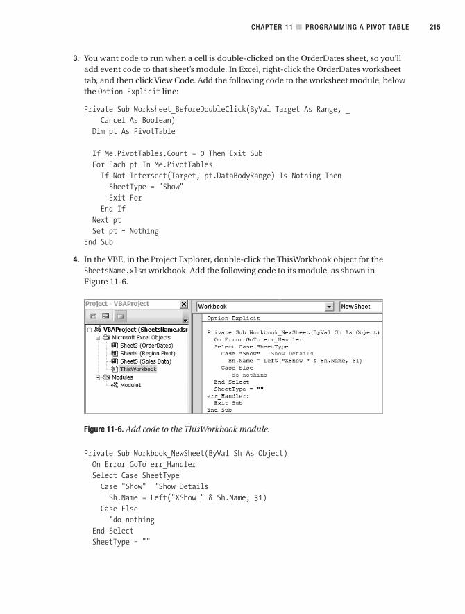
3. You want code to run when a cell is double-clicked on the OrderDates sheet, so you’lladd event code to that sheet’s module. In Excel, right-click the OrderDates worksheettab, and then click View Code. Add the following code to the worksheet module, belowthe Option Explicit line:

Private Sub Worksheet_BeforeDoubleClick(ByVal Target As Range, _Cancel As Boolean)

Dim pt As PivotTable

If Me.PivotTables.Count = 0 Then Exit SubFor Each pt In Me.PivotTablesIf Not Intersect(Target, pt.DataBodyRange) Is Nothing ThenSheetType = "Show"Exit For

End IfNext ptSet pt = Nothing

End Sub

4. In the VBE, in the Project Explorer, double-click the ThisWorkbook object for theSheetsName.xlsm workbook. Add the following code to its module, as shown in Figure 11-6.

Figure 11-6. Add code to the ThisWorkbook module.

Private Sub Workbook_NewSheet(ByVal Sh As Object)On Error GoTo err_HandlerSelect Case SheetTypeCase "Show" 'Show DetailsSh.Name = Left("XShow_" & Sh.Name, 31)

Case Else'do nothing

End SelectSheetType = ""


err_Handler:Exit Sub

End Sub

To run the event code, double-click a cell in the OrderDates pivot table’s Values area. Aworksheet is created with the extracted data, and a sheet name that starts with XShow_.

How It WorksWhen any cell on the pivot table’s sheet is double-clicked, the BeforeDoubleClick event is trig-gered. If no pivot tables are on the worksheet, or if the double-clicked cell is not in the Valuesarea (pt.DataBodyRange) of a pivot table, the procedure is exited. Otherwise, the public vari-able, SheetType, is set to a value of Show. If the double-click creates a new sheet, the workbook’sNewSheet event code runs.

If SheetType is set to the value of Show, the sheet is given a name that starts with XShow_.This makes the sheets easy to identify, and they can be deleted automatically when the work-book closes. See Section 11.6 for sample code to delete the worksheets.

11.6. Automatically Deleting Worksheets When Closinga Workbook

ProblemOnce a week, you send a printed copy of the Region Pivot report to the manager of eachregion. On the Ribbon’s Options tab, in the PivotTable group, you can click the Options drop-down arrow, and then click Show Report Filter Pages, to create a worksheet with a copy of thepivot table for each region in the Report Filter Field.

This command is useful for printing customized copies of the pivot table, but it adds extrasheets to the workbook. You’d like these sheets to be automatically deleted when the work-book is closed to prevent the buildup of sheets. This problem is based on theSheetsDelete.xlsm sample workbook.

SolutionYou can use an event procedure that runs when a sheet is added to the workbook to renamethe new sheets, so they’re easy to identify and delete when the workbook closes.

1. In the ThisWorkbook module, add the following two procedures:

Private Sub Workbook_NewSheet(ByVal Sh As Object)If TypeName(Sh)="Worksheet" ThenIf Sh.PivotTables.Count > 0 ThenIf Sh.PivotTables(1).PageFields.Count > 0 ThenSh.Name = Left("XShow_" & Sh.Name, 31)

End IfEnd If

End If


End Sub'Private Sub Workbook_BeforeClose(Cancel As Boolean)Dim ws As WorksheetDim Resp As LongDim ShowCount As Long

ShowCount = 0For Each ws In ThisWorkbook.WorksheetsIf UCase(Left(ws.Name, 5)) = "XSHOW" ThenShowCount = ShowCount + 1

End IfNext ws

If ShowCount > 0 ThenResp = MsgBox("Delete Show Report Filter Pages sheets?", _

vbYesNo, "Delete Sheets?")If Resp = vbYes ThenApplication.DisplayAlerts = FalseFor Each ws In ThisWorkbook.WorksheetsIf UCase(Left(ws.Name, 5)) = "XSHOW" Thenws.Delete

End IfNext ws

End IfEnd IfSet ws = Nothing

End Sub

2. To run the event code that names the sheets, select a cell in the pivot table and on theRibbon’s Options tab, in the PivotTable group, click the Options drop-down arrow, andthen click Show Report Filter Pages. Select a report filter in the list, and then click OK.

How It WorksIf a new sheet is created, the workbook’s NewSheet event is triggered. If the new sheet containsa pivot table, and that pivot table has a report filter, it’s assumed to be generated by the ShowReport Filter Pages command. The sheet is renamed by the NewSheet code, with XShow_ atthe start of the name.

When the workbook closes, the workbook’s BeforeClose event is triggered. The event codeasks the user if Show Report Filter Pages sheets should be deleted. If the user clicks Yes, thesheets are deleted, and the workbook can be saved without the sheets.

NotesThe ThisWorkbook module can contain only one copy of each event, such as theWorkbook_NewSheet event. To use both the sample code from Section 11.5 and the samplecode in this section, you can combine the Workbook_NewSheet code into one procedure:


Private Sub Workbook_NewSheet(ByVal Sh As Object)On Error GoTo err_HandlerSelect Case SheetTypeCase "Show" 'Show DetailsSh.Name = Left("XShow_" & Sh.Name, 31)

Case Else'do nothing

End SelectSheetType = ""

If TypeName(Sh) = "Worksheet" ThenIf Sh.PivotTables.Count > 0 ThenIf Sh.PivotTables(1).PageFields.Count > 0 ThenSh.Name = Left("XShow_" & Sh.Name, 31)

End IfEnd If

End If

err_Handler:Exit Sub

End Sub

11.7. Changing the Report Filter Selection in Related Tables

ProblemIn your workbook, three pivot tables are based on the same Excel Table, and the Product fieldis in the Report Filter area for each pivot table. When you’re asked for the status of a specificproduct, you select that product from the report filter in each pivot table, and you print allthree pivot tables.

It would be easier if you could change the Product Report Filters in all the pivot tables atthe same time, instead of going to each sheet and changing them individually. This problem isbased on the ChangeTwo.xlsm sample workbook.

SolutionYou can use an event procedure to change the other pivot tables’ report filters when the Prod-uct report filter is changed in the OrderDates pivot table.

1. Right-click the sheet tab for the OrderDates pivot table, and then click View Code.

2. Enter the following line of code in the General Declarations section at the top of themodule (see Figure 11-7). This is a module-level variable:

Dim mstrFilter As Variant


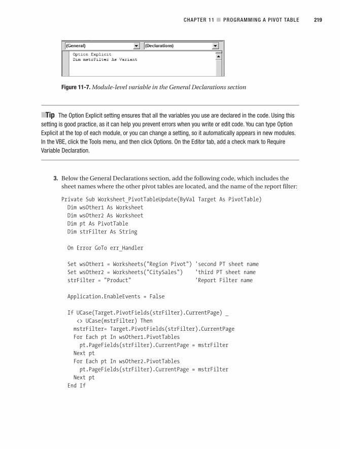
Figure 11-7. Module-level variable in the General Declarations section

■Tip The Option Explicit setting ensures that all the variables you use are declared in the code. Using thissetting is good practice, as it can help you prevent errors when you write or edit code. You can type OptionExplicit at the top of each module, or you can change a setting, so it automatically appears in new modules.In the VBE, click the Tools menu, and then click Options. On the Editor tab, add a check mark to RequireVariable Declaration.

3. Below the General Declarations section, add the following code, which includes thesheet names where the other pivot tables are located, and the name of the report filter:

Private Sub Worksheet_PivotTableUpdate(ByVal Target As PivotTable)Dim wsOther1 As WorksheetDim wsOther2 As WorksheetDim pt As PivotTableDim strFilter As String

On Error GoTo err_Handler

Set wsOther1 = Worksheets("Region Pivot") 'second PT sheet nameSet wsOther2 = Worksheets("CitySales") 'third PT sheet name strFilter = "Product" 'Report Filter name

Application.EnableEvents = False

If UCase(Target.PivotFields(strFilter).CurrentPage) _<> UCase(mstrFilter) ThenmstrFilter= Target.PivotFields(strFilter).CurrentPageFor Each pt In wsOther1.PivotTablespt.PageFields(strFilter).CurrentPage = mstrFilter

Next ptFor Each pt In wsOther2.PivotTablespt.PageFields(strFilter).CurrentPage = mstrFilter

Next ptEnd If


err_Handler:Application.EnableEvents = True

End Sub

To run the event code, change the selection in the OrderDates pivot table’s report filter.

How It WorksA variable within a procedure is stored only as long as the procedure that declared it is run-ning. A module-level variable is used in this example, because it can store the current reportfilter selection while the workbook is open. When the pivot table is updated, the variablenamed mstrFilter is compared to the current selection in the Product Report Filter. If they’redifferent, the new report filter value is stored in the variable, and the report filter in eachrelated pivot table is changed to match the report filter in the main pivot table.

11.8. Removing Filters in a Pivot Field

ProblemWhen you want to remove a filter from a pivot table field, you can manually check the ShowAll box to show all items in that pivot table field. When you record this step, the code shows alist of all the items in the pivot field, instead of using a Show All command. When you run thecode later, it can be very slow, if the list of items is long, such as in an OrderDate field. Also, ifyou add new items to the field and run the macro, the new items aren’t made visible, becausethe macro contains a list of the original items only. This problem is based on the Filters.xlsmsample workbook.

SolutionInstead of using the recorded code, with its long list of items, you can use theClearManualFilter method. For example, the following code shows all items, in all visiblefields, in all tables on the active sheet. Store the code on a regular module.

Sub ClearFilters ()Dim pt As PivotTableDim pf As PivotFieldDim ws As Worksheet

On Error GoTo err_Handler

Set ws = ActiveSheet

Application.ScreenUpdating = FalseApplication.DisplayAlerts = False


For Each pt In ws.PivotTablesFor Each pf In pt.VisibleFieldsOn Error Resume Nextpf.ClearManualFilter

Next pfNext pt

exit_Handler:Application.ScreenUpdating = TrueExit Sub

err_Handler:MsgBox Err.Number & ": " & Err.DescriptionGoTo exit_HandlerSet pf = NothingSet pt = NothingSet ws = Nothing

End Sub

To run the code, use a method described in Section 11.1. The code refers to ActiveSheet, soyou can run the code on any sheet that contains a pivot table.

How It WorksThe ClearFilters code uses For Each...Next loops to clear the manual filters in all visible fields,in all pivot tables on the active worksheet.

■Tip To show only column fields, change pt.VisibleFields to pt.ColumnFields. To show only therow fields, change pt.VisibleFields to pt.RowFields, and to show report filter fields, changept.RowFields to pt.PageFields.

The ClearManualFilter method only clears the manual filters applied to the pivot field.You apply a manual filter by using the check boxes in the filter list, or by right-clicking an item,clicking Filter, and then clicking Hide Selected Items.

In addition to the manual filters, date, value, or label filters may have been applied to therow or column fields.

To clear value or Top 10 filters, you can use the following method:

pf.ClearValueFilters

To clear label or date filters, you can use the following method:

pf.ClearLabelFilters


To clear all filters in the pivot table, you can use the following method:

For Each pt In ws.PivotTablespt.ClearAllFilters

Next pt

■Tip While recording a macro, you can record the ClearAllFilters method. Right-click a filtered field, clickFilter, and then click Clear Filter from FieldName.

11.9. Changing Content in the Values Area

ProblemYou discovered that one of the totals in your OrderDates report is incorrect, but you haven’treceived the corrected source data yet. You need to print the totals for the sales manager, who’sleaving for the airport in 15 minutes. As a temporary fix, you’d like to change the New Yorktotal and the Grand Total in the Values area of the pivot table, so you can print the report.

However, when you try to type over a value, you see the error message “Cannot changethis part of a PivotTable report.” This problem is based on the Change.xlsm sample workbook.

SolutionThe best solution is to add a row in the source data, to adjust the New York total, with a com-ment to explain the entry. Then, refresh the pivot table, to see the updated total. After thecorrected source data is received, another row can be added, to reverse the temporary adjust-ment. This solution would leave an audit trail, explaining the changes.

However, if you change a PivotTable setting programmatically, you can make temporarychanges to the PivotTable values. Store the code in a regular code module.

Sub ChangePTValues()Dim pt As PivotTable

Set pt = ActiveSheet.PivotTables(1)pt.EnableDataValueEditing = TrueSet pt = Nothing

End Sub

■Note When the pivot table is refreshed, the manually entered values are overwritten.

To run the code, use a method described in Section 11.1. The code refers to ActiveSheet,so you can run the code on any sheet that contains a pivot table.


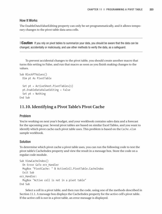
How It WorksThe EnableDataValueEditing property can only be set programmatically, and it allows tempo-rary changes to the pivot table data area cells.

■Caution If you rely on pivot tables to summarize your data, you should be aware that the data can bechanged, accidentally or maliciously, and use other methods to verify the data, as a safeguard.

To prevent accidental changes to the pivot table, you should create another macro thatturns this setting to False, and run that macro as soon as you finish making changes to thevalues.

Sub BlockPTValues()Dim pt As PivotTable

Set pt = ActiveSheet.PivotTables(1)pt.EnableDataValueEditing = FalseSet pt = Nothing

End Sub

11.10. Identifying a Pivot Table’s Pivot Cache

ProblemYou’re working on next year’s budget, and your workbook contains sales data and a forecastfor the upcoming year. Several pivot tables are based on similar Excel Tables, and you want toidentify which pivot cache each pivot table uses. This problem is based on the Cache.xlsmsample workbook.

SolutionTo determine which pivot cache a pivot table uses, you can run the following code to test thepivot table’s CacheIndex property and view the result in a message box. Store the code on aregular code module.

Sub ViewCacheIndex()On Error GoTo err_HandlerMsgBox "PivotCache: " & ActiveCell.PivotTable.CacheIndexExit Sub

err_Handler:MsgBox "Active cell is not in a pivot table"

End Sub

Select a cell in a pivot table, and then run the code, using one of the methods described inSection 11.1. A message box displays the CacheIndex property for the active cell’s pivot table.If the active cell is not in a pivot table, an error message is displayed.


How It WorksWhen pivot caches are created, they are added to the workbook’s PivotCaches collection andgiven an index number. This number is displayed in the macro’s message box. If a pivot tableis based on the same source data as an existing pivot table, it uses the same pivot cache.

11.11. Changing a Pivot Table’s Pivot Cache

ProblemYou used the code from Section 11.10 to identify the pivot cache used by each pivot table inyour workbook. You want to change the pivot cache of the Category pivot table, so it uses thesame cache as the StoreTotals pivot table. This problem is based on the Cache.xlsm sampleworkbook.

SolutionTo change the pivot cache, you can set the pivot table’s CacheIndex property. The followingcode sets the pivot table for the active cell to use pivot cache number 2. Store the code on aregular code module.

Sub SetCache2Index()On Error GoTo err_HandlerActiveCell.PivotTable.CacheIndex = 2Exit Sub

err_Handler:MsgBox "Cache index could not be changed"

End Sub

To run the code, use a method described in Section 11.1. The code refers to ActiveCell, so youcan run the code on any sheet that contains a pivot table.

How It WorksThe SetCache2Index code sets the CacheIndex property for the active cell’s pivot table to 2. If a pivot table cell is not selected, or if there is no CacheIndex 2, an error message is displayed.Instead of setting the CacheIndex property to a specific number, you can obtain an indexnumber in the code, and use that number as the setting. For example:

Sub SetCacheIndex()Dim i As Integeri = Worksheets("StoreTotals").PivotTables(1).CacheIndexOn Error GoTo err_HandlerActiveCell.PivotTable.CacheIndex = iExit Sub

err_Handler:MsgBox "Cache index could not be changed"

End Sub


11.12. Refreshing a Pivot Table on a Protected Sheet

ProblemYou protected the StoreTotals worksheet, so no one is able to change the layout of the pivottable. Now, you want to refresh the StoreTotals pivot table, but the Refresh Data button on thePivotTable toolbar is disabled. This problem is based on the Refresh.xlsm sample workbook.

SolutionYou can record a macro, modify it slightly, and then run that macro when you need to refreshthe pivot table. Before you begin, protect the StoreTotals worksheet, with the password pwd.

1. Record a macro as you unprotect the StoreTotals sheet, refresh the pivot table, andthen protect the worksheet.

2. View the recorded code in the VBE. For example, your code may look similar to thefollowing:

Sub RefreshPivot()ActiveSheet.UnprotectRange("B1").SelectActiveSheet.PivotTables("StorePT").PivotCache.RefreshActiveSheet.Protect DrawingObjects:=True, _Contents:=True, Scenarios:=True

End Sub

3. In the recorded code, you can add a password to the Unprotect and Protect lines. Forexample, if your password is pwd, the revised code would be as follows:

Sub RefreshPivot()ActiveSheet.Unprotect Password:="pwd"Range("B1").SelectActiveSheet.PivotTables("StorePT").PivotCache.RefreshActiveSheet.Protect Password:="pwd", _DrawingObjects:=True, Contents:=True, Scenarios:=True

End Sub

4. Run the macro using one of the methods shown in Section 11.1.

How It WorksThe RefreshPivot macro stores your password, and then uses it when unprotecting and pro-tecting the worksheet. While the worksheet is unprotected, it refreshes the pivot table.


NotesIf you add your password to the macro, it is visible to anyone who can open your workbookproject in the VBE. For information on protecting your code, see the article “Locking YourSolution’s VBA Project,” at http://msdn2.microsoft.com/en-us/library/Aa165442(office.10).aspx.

Although the article refers to Excel 2000, it is still applicable to a VBA project in Excel 2007.

11.13. Refreshing Automatically When Source Data Changes

ProblemYou frequently update the source data that’s in an Excel Table in your workbook, but you for-get to update the pivot table that’s based on it. Hours later, you realize you printed severalreports, all of which contain outdated information. To avoid wasting time and paper, youwant the pivot table to automatically refresh when changes are made in the Excel Table onwhich the pivot table is based. This problem is based on the Update.xlsm sample workbook.

SolutionYou can use an event procedure to automatically update the pivot table if the source datachanges. In this example, the source data is on the Forecast sheet, and the pivot table is on theProduct sheet:

1. Add the following code to the Forecast worksheet module:

Private Sub Worksheet_Change(ByVal Target As Range)Worksheets("Product").PivotTables(1).PivotCache.Refresh

End Sub

2. If you protected the Product worksheet, include code to unprotect the worksheet, andthen protect it again, as shown in Section 11.12.

3. To run the event code, make a change to the data in the Excel Table.

How It WorksWhen a change is made on the Forecast worksheet, that sheet’s Change event is triggered. Inthe Event code, the pivot cache for the Product sheet’s pivot table is refreshed.

11.14. Setting a Minimum Width for Data Bars

ProblemYou created a pivot table to show the quantity of snacks sold each month, and you added con-ditional formatting, using the data bars option. Although zero were sold in March and onlyone sold in April, the data bars for those months are too wide, in proportion to the other bars.You changed the setting for the Lowest Value, as described in Section 4.17, but the bars are stilltoo wide. You’d like to fix the data bars, so the bars that represent zero and one are barely visi-ble. This problem is based on the DataBars.xlsm sample file.


SolutionAlthough you can adjust the Lowest Value setting in the Edit Formatting Rule dialog box, youcan’t change the size of the smallest bar, which will be approximately 10 percent the width ofthe bar for the highest value.

However, the minimum width can be adjusted programmatically. For example, you canchange the minimum width to 1 percent, and the bars for the zero and one will be much nar-rower (see Figure 11-8).

Figure 11-8. The minimum width for data bars is reduced to 1 percent.

In the following code, the minimum width of the data bars that start in cell B6 will bechanged to 1 percent. Also, the Lowest Value will be set as a Number, with zero as the value.You can manually change this setting in the Edit Formatting Rules dialog box, but it isincluded here for convenience.

Sub DataBarWidth()

With Range("B6").FormatConditions(1).MinPoint.Modify _

NewType:=xlConditionValueNumber, NewValue:=0.PercentMin = 1

End With

End Sub

11.15. Preventing Selection of (All) in a Report Filter

ProblemYou’re sending a copy of your workbook to the regional managers. In the OrderDates pivottable, you want the managers to view the sales totals by selecting an order date. GetPivotDataformulas are on the worksheet that will result in an error if (All) is selected, so you want to pre-vent them from choosing (All) in the report filter’s drop-down list. This problem is based onthe BlockAll.xlsm sample workbook.


SolutionYou can’t remove the (All) option from the report filter’s drop-down list, but you can use pro-gramming to prevent users from selecting that option. The following code, stored on theOrderDates sheet’s module, can undo the report filter change, if (All) is selected or if multipleitems are selected in the filter, and displays a message warning:

Private Sub Worksheet_PivotTableUpdate(ByVal Target As PivotTable)Dim pf As PivotFieldOn Error GoTo exit_Handler

Application.EnableEvents = FalseApplication.ScreenUpdating = False

For Each pf In Target.PageFieldsIf pf.CurrentPage = "(All)" Then

Application.UndoMsgBox "Please select a single date."

End IfNext pf

exit_Handler:Set pf = NothingApplication.EnableEvents = TrueApplication.ScreenUpdating = True

End Sub

To run the code, select (All) from the OrderDate report filter’s drop-down list.

How It WorksWhen an item is selected from a report filter’s drop-down list, the PivotTableUpdate event istriggered. If the (All) item was selected, the code undoes the change to the report filter, anddisplays the previously selected item.

11.16. Disabling Pivot Field Drop-Downs

ProblemIn the workbook you’re sending to regional managers, you selected the manager’s region namefrom the report filter on the Region Pivot worksheet, and all the stores in their region are in theRow Labels area. To ensure they’re viewing the correct data, you want to prevent the managersfrom selecting a different item in the report filter or in the Row Labels filters. This problem isbased on the Protect.xlsm sample workbook.


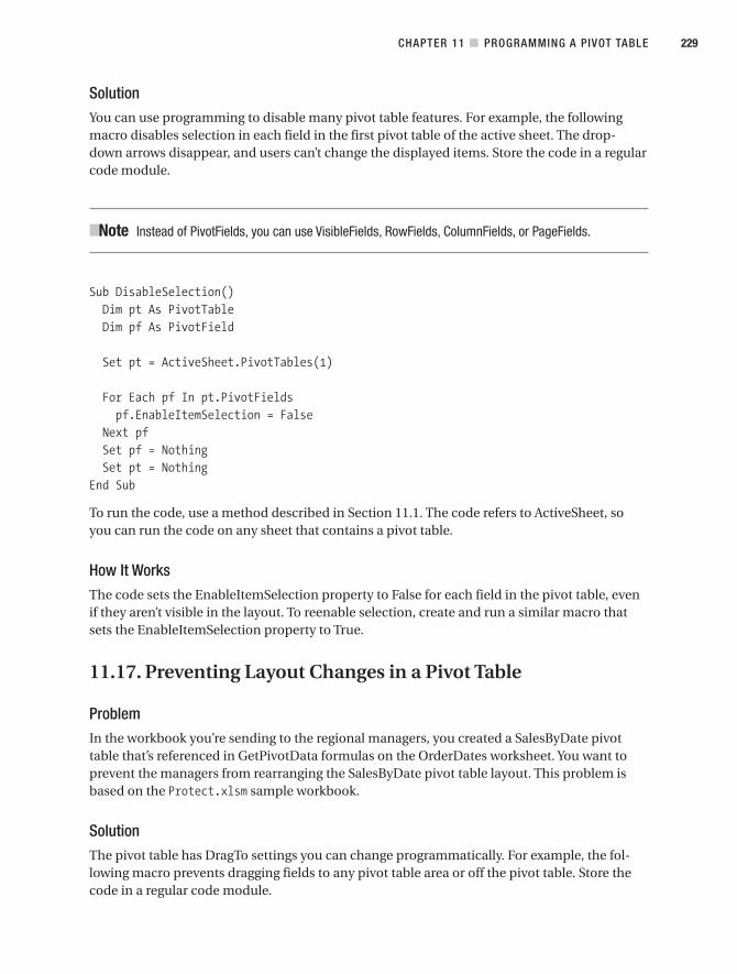
SolutionYou can use programming to disable many pivot table features. For example, the followingmacro disables selection in each field in the first pivot table of the active sheet. The drop-down arrows disappear, and users can’t change the displayed items. Store the code in a regularcode module.

■Note Instead of PivotFields, you can use VisibleFields, RowFields, ColumnFields, or PageFields.

Sub DisableSelection()Dim pt As PivotTableDim pf As PivotField

Set pt = ActiveSheet.PivotTables(1)

For Each pf In pt.PivotFieldspf.EnableItemSelection = False

Next pfSet pf = NothingSet pt = Nothing

End Sub


How It WorksThe code sets the EnableItemSelection property to False for each field in the pivot table, evenif they aren’t visible in the layout. To reenable selection, create and run a similar macro thatsets the EnableItemSelection property to True.

11.17. Preventing Layout Changes in a Pivot Table

ProblemIn the workbook you’re sending to the regional managers, you created a SalesByDate pivottable that’s referenced in GetPivotData formulas on the OrderDates worksheet. You want toprevent the managers from rearranging the SalesByDate pivot table layout. This problem isbased on the Protect.xlsm sample workbook.

SolutionThe pivot table has DragTo settings you can change programmatically. For example, the fol-lowing macro prevents dragging fields to any pivot table area or off the pivot table. Store thecode in a regular code module.


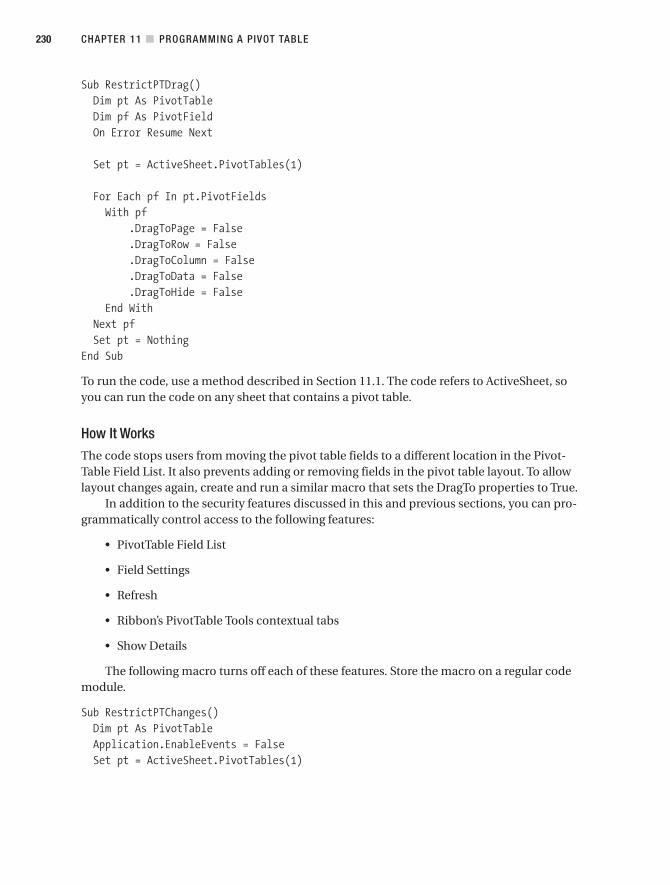
Sub RestrictPTDrag()Dim pt As PivotTableDim pf As PivotFieldOn Error Resume Next

Set pt = ActiveSheet.PivotTables(1)

For Each pf In pt.PivotFieldsWith pf

.DragToPage = False

.DragToRow = False

.DragToColumn = False

.DragToData = False

.DragToHide = FalseEnd With

Next pfSet pt = Nothing

End Sub


How It WorksThe code stops users from moving the pivot table fields to a different location in the Pivot-Table Field List. It also prevents adding or removing fields in the pivot table layout. To allowlayout changes again, create and run a similar macro that sets the DragTo properties to True.

In addition to the security features discussed in this and previous sections, you can pro-grammatically control access to the following features:

• PivotTable Field List

• Field Settings

• Refresh

• Ribbon’s PivotTable Tools contextual tabs

• Show Details

The following macro turns off each of these features. Store the macro on a regular codemodule.

Sub RestrictPTChanges()Dim pt As PivotTableApplication.EnableEvents = FalseSet pt = ActiveSheet.PivotTables(1)


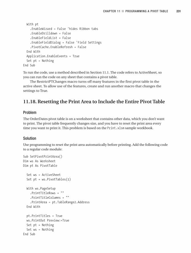
With pt.EnableWizard = False 'hides Ribbon tabs.EnableDrilldown = False.EnableFieldList = False.EnableFieldDialog = False 'Field Settings.PivotCache.EnableRefresh = False

End With Application.EnableEvents = TrueSet pt = Nothing

End Sub


The RestrictPTChanges macro turns off many features in the first pivot table in theactive sheet. To allow use of the features, create and run another macro that changes thesettings to True.

11.18. Resetting the Print Area to Include the Entire Pivot Table

ProblemThe OrderDates pivot table is on a worksheet that contains other data, which you don’t wantto print. The pivot table frequently changes size, and you have to reset the print area everytime you want to print it. This problem is based on the Print.xlsm sample workbook.

SolutionUse programming to reset the print area automatically before printing. Add the following codeto a regular code module:

Sub SetPivotPrintArea()Dim ws As WorksheetDim pt As PivotTable

Set ws = ActiveSheetSet pt = ws.PivotTables(1)

With ws.PageSetup.PrintTitleRows = "".PrintTitleColumns = "".PrintArea = pt.TableRange2.Address

End With

pt.PrintTitles = Truews.PrintOut Preview:=TrueSet pt = NothingSet ws = Nothing

End Sub



How It WorksThe SetPivotPrintArea macro clears the print titles for the active sheet, sets the print areabased on the current layout of the pivot table, turns on the pivot table’s print titles options,and prints the worksheet. In this example, the ws.PrintOut line has Preview set to True, so theworksheet will preview instead of printing. When you finish testing the code, you can changethe setting to False, and the sheet will print when the code runs.

11.19. Printing the Pivot Table for Each Report Filter Field

ProblemYou’re preparing for a sales meeting, and you want to print a copy of the pivot table foreach item in the Category report filter. This problem is based on the PrintCat.xlsm sampleworkbook.

SolutionThe following code prints the pivot table once for each item in the Category report filter.Store the code in a regular code module.

Sub PrintPivotFilters()Dim pt As PivotTableDim pf As PivotFieldDim pi As PivotItemDim ws As WorksheetOn Error Resume Next

Set ws = ActiveSheetSet pt = ws.PivotTables(1)Set pf = pt.PageFields("Category")

For Each pi In pf.PivotItemspf.CurrentPage = pi.Namews.PrintOut Preview:=True

Next pi

Set pf = NothingSet pt = NothingSet ws = Nothing

End Sub



How It WorksThe PrintPivotFilters macro selects each item in the pivot table’s first report filter, and thenprints the worksheet. In this example, the ws.PrintOut line has Preview set to True, so theworksheet will preview instead of printing. When you finish testing the code, you can changethe setting to False, and the sheet will print when the code runs.

NotesThe procedure can be modified slightly to print a copy of a pivot chart on a chart sheet foreach item in the Category report filter. Store the code on a regular code module.

Sub PrintPivotChartFilters()Dim pt As PivotTableDim pf As PivotFieldDim pi As PivotItemDim ch As ChartOn Error Resume Next

Set ch = ActiveChartSet pt = ch.PivotLayout.PivotTableSet pf = pt.PageFields("Category")

For Each pi In pf.PivotItemspf.CurrentPage = pi.Namech.PrintOut Preview:=True

Next pi

Set ch = NothingSet pf = NothingSet pt = Nothing

End Sub

11.20. Scrolling Through Report Filter Items on a Pivot Chart

ProblemOn the OrderDates Chart sheet, you have a list of categories in the Pivot Chart report filter.Instead of selecting the next category from the drop-down list to view its chart, you’d likescrolling buttons on the chart, so you can quickly view each category’s data. This problem isbased on the PrintCat.xlsm sample workbook.

SolutionYou can add arrow shapes to the chart, and assign a macro to each shape, and then click thearrows to select the next or previous report filter item.


1. Add the following two procedures to a regular code module:

Sub PivotPageNext()Dim CountPI As LongDim i As LongDim pt As PivotTableDim pf As PivotFieldDim pi As PivotItem

Set pt = ActiveChart.PivotLayout.PivotTableSet pf = pt.PageFields("Category")CountPI = 1i = 1

For Each pi In pf.PivotItemsIf pf.CurrentPage.Name = "(All)" ThenCountPI = 0Exit For

End IfIf pi.Name = pf.CurrentPage.Name Then

Exit ForEnd IfCountPI = CountPI + 1

Next pi

For i = CountPI + 1 To pf.PivotItems.Count + 1On Error Resume NextIf i = pf.PivotItems.Count + 1 Thenpf.CurrentPage = "(All)"Exit For

End Ifpf.CurrentPage = pf.PivotItems(i).NameIf Err.Number = 0 ThenExit For

End IfNext iSet pf = NothingSet pt = Nothing

End Sub

Sub PivotPagePrev()Dim CountPI As LongDim i As LongDim pt As PivotTableDim pf As PivotFieldDim pi As PivotItem


Set pt = ActiveChart.PivotLayout.PivotTableSet pf = pt.PageFields("Category")CountPI = 1

For Each pi In pf.PivotItemsIf pf.CurrentPage.Name = "(All)" ThenCountPI = pf.PivotItems.Count + 1Exit For

End IfIf pi.Name = pf.CurrentPage.Name Then Exit ForCountPI = CountPI + 1

Next pi

For i = CountPI - 1 To 0 Step -1On Error Resume Nextpf.CurrentPage = pf.PivotItems(i).NameIf Err.Number = 0 Then Exit For

If i = 0 Thenpf.CurrentPage = "(All)"Exit For

End IfNext iSet pf = NothingSet pt = Nothing

End Sub

2. Select the OrderDates Chart sheet, and on the Ribbon’s Insert tab, in the Illustrationsgroup, click Shapes.

3. Click the Left Arrow shape, and then click the chart, to add that shape.

4. On the chart, right-click the Left Arrow shape, and then click Assign Macro.

5. In the list of macros, select PivotPagePrev, and then click OK.

6. Add a Right Arrow shape, and assign it the PivotPageNext macro.

7. To scroll through the report filter items, click the arrows (see Figure 11-9).

Figure 11-9. Scrolling arrows at the top of a pivot chart


How It WorksThe two macros check the current report filter item and calculate its position in the list ofitems. If the Left Arrow shape is clicked, the PivotPagePrev macro runs, and the visible itemwith the next lower number is shown. If the Right Arrow shape is clicked, the PivotPageNextmacro runs, and the visible item with the next higher number is shown.


■symbols% Difference From custom calculation, 49, 65% of Column custom calculation, 53% Of custom calculation, 48% of Row custom calculation, 52% of Total custom calculation, 54< less than symbol, 92> greater than symbol, 92[ ] square brackets, 181* wildcard, 29? wildcard, 29

■AAccess queries

preparing source data and, 13source file and, 146

adding items, with calculated items, 57Advanced Filters, 9amounts, calculating percent difference

between, 64applying PivotTable styles, 72area charts, 191ascending sorts, 22AutoFilters, 9Average summary function, 43AVERAGE worksheet function, 43axis title, 200

■Bbar charts, 191Between filter, 28black-and-white printing, 173blank cells, counting, 45blank rows, as separations for field items, 96Bottom 10 filtering, 36Bottom 10 Items conditional formatting

option, 84Bubble charts, 191, 193buttons

hiding, 81scrolling, for pivot charts, 233

■Ccalculated fields, 56–67

vs. calculated items, 56correcting results in, 67creating, 61count of unique items, 66

grand total, correcting for, 65identifying, 63list of, creating, 67modifying, 62removing, 63

calculated items, 56–69adding to fields with grouped items, 64vs. calculated fields, 56created accidentally, 67errors messages and, 105identifying, 63index numbers, using, 59list of, creating, 67, 105modifying, 58, 60removing, 59with no data, hiding, 135

calculations, 41–69custom, 46–56formulas and, 56–69summary functions and, 41–45

captions, hiding, 81Cartesian products, 135categories, sorting, 21category axis, of pivot charts, 189cell references, 179–182cells

Highlight Cell Rules option and, 85Merge and Center Cells with Labels option

and, 97changing. See editingcharts. See pivot chartschart templates, 194chart title, 199cities, sorting, 21, 24“Client Safety options…” error message, 152Collapse/Expand indicator, 131collapsing

items in selected fields, 131row labels, 130

color scales, 81, 87column charts, 191column headings

freezing, 98repeating across pages, 167

column labels, 9, 16blank, adding N/A to, 133filters for, 30subtotals and, 118

column width, lost formatting and, 79

Index

237

columns% of Column custom calculation and, 53Index custom calculation and, 55monthly, 9new, automatically including with source

data, 141organizing data in, 4

comments, adding to pivot table cells, 129common filters, 32Compact Form, 93conditional formatting, 81–92

between two values, 85bottom 10 items, 84color scale, 81data bars, 87, 226data range, changing, 89date period, 86icon set, 82order of rules, changing, 91pivot charts and, 198removing (clearing), 92

connections, enabling, 156Contains filter, 29contextual tooltips, 129Count Numbers summary function, 43, 44Count summary function, 41, 43, 213

blank cells and, 45source data errors and, 44

COUNT worksheet function, 43COUNTA worksheet function, 43COUNTIF formula, 66Create a Single Page Field for Me option, 17creating

calculated items/calculated fields, 61, 105chart templates, 194custom lists, 25custom PivotTable styles, 74customized copies of pivot tables, 187Excel Tables, 6lists of formulas, 67pivot charts, 189–196, 203pivot tables, 1–20

current month, conditional formatting for, 86custom calculations, 46-56custom lists, 25, 27custom number formats, 92custom order, sorting in, 25

■Ddata

creating pivot tables from, 15extracting, 173–186grouping/totaling, 101–121normalizing 11–12organizing in rows/columns, 4preparing source data and, 4, 8

data bars, 87, 226

data connections, enabling, 156database password, storing in connection

string, 155date filters, 28, 30, 32dates

current month, conditional formatting for,86

data ranges, filtering for, 38errors and, 185filtering data by, 31formatted, summarizing, 112future, filtering for, 38grouping, 101, 104, 107–113, 134nonconsecutive, 33pivot charts and, 201Report Filter formatting and, 98Running Total custom calculation and, 51subtotal labels and, 99

default PivotTable style, changing, 74deleting. See removingdifference between amounts, calculating, 64Difference From custom calculation, 46disabling

pivot table features, 228security features, 230Show Details feature, 230Show Report Filter Pages feature, 160

displayingall field items, 134multiple value fields, 114seconds, hundredths of, 121subtotals, 115, 118

districts, sorting, 8, 21Document Themes, 77Does Not End With filter, 29doughnut charts, 191Down, Then Over option, Report Filters and,

125drag-and-drop functionality, 137drop-downs, disabling, 228dynamic filters, 32

■Eediting

calculated fields, 62calculated item formulas in cells, 60calculated items, 58default PivotTable style, 74grand total label text, 100layouts, 93, 229order of rules, 91pivot tables, 123–138ranges of data, 89Report Layouts, 93source Access file, 146source CSV file, 147source Excel Table, 145

■INDEX238

subtotal date format, 99subtotal label text, 99

electronic format, sharing information and, 3empty cells, showing zero, 80Enable Selection option, 78, 97error values, hiding, 79errors

calculated items and, 105custom subtotals and, 183dates and, 101, 185Excel Field Names Not Valid, 8GetPivotData formulas and, 179GetPivotData function and, 182–186numbers groupings and, 102missing items and, 182OLAP cubes and, 152pivot charts and, 194PivotTable reports and, 222

event code, 206Excel 2007

new functions with, 71, 183object model and, 205

Excel Field Names Not Valid error message, 8Excel Lists (Excel 2003), 6, 15, 18Excel Macro-Enabled Workbooks, 205Excel Tables, 6

preparing source data and, 6, 9source, 139, 144

external ranges of data, 143extracted data

deleting sheets created, 176formatting, 175

extracting data, 173–186extracting underlying data, 173

■Ffield items

blank, extracting data for, 182displaying all, 134printing each on a new page, 172separating with blank rows, 96

field labels, centering vertically, 96field list order, 20field names

showing on pivot charts, 199changing in source data, 132

fieldssource data and, 2using multiple, 113

file size, reducing, 164filter lists, clearing old items from, 132filtered data, preparing source data and, 8filtering

by selection, 35date range, 38nonconsecutive dates, 33pivot charts, 195

pivot tables, 28–37row field values, 32top items, 36

filtersclearing old items from, 132for dates, 32for row labels, 30manual filter, including new items, 34multiple filters, applying, 29removing from pivot fields, 220report filter items, hiding, 37row label text, 28using more than one at a time, 29

fiscal quarter, grouping dates by, 108formatting

extracted data, 175hyperlinks, 98losing when refreshing, 79pivot charts and, 198pivot tables, 71–100

formulas, 56–69automatic insertion for, 176changing Solve Order and, 68creating list of, 67determining type of, 63

freezing column/row headings, 98functions, new with Excel 2007, 183future dates, filtering for, 38

■GGetPivotData function, 167, 176–186

blank field items, 183cell references and, 179–182custom subtotals, 183date references, 185errors and, 182–186missing items, 182referencing other workbooks, 179referring to a pivot table, 186turning off, 178value fields, cell references, 182

grand total valueschanging label text for, 100correcting for calculated field, 65filtering, 32hiding specific, 120simulating an additional, 119

greater than (>), custom number formatsand, 92

Group Selection command, 106grouping

another pivot table affected, 110calculated items, error message, 105data, 101–113dates, 104, 107–113, 134dates by month, 107dates outside the range, 112

■INDEX 239

Finditfasterathttp://superindex.apress.com

/

error message, 101fiscal quarter, 108months and weeks, 110numbers, 102report filter, 104showing all months, 134starting date, 107text items, 106

■Hheading cells, blank, 8heading rows, freezing, 98headings, repeating across pages, 167hiding

buttons, 81error values, 79grand total values, 120items, 16, 36, 37, 135labels/captions, 81

highest valuesdata bars for, 87highlighting, 81

Highlight Cell Rules conditional formattingoption, 85

hours, totaling, 121hyperlinks, formatting, 98

■II Will Create the Page Fields option, 17icon sets, 82, 87IFERROR function, 183indentation, for row labels, 94Index custom calculation, 55INDEX function, 143index numbers, in calculated items, 59INDIRECT function, 186Information Rights Management, 3inner fields, 21innermost fields, row/column label subtotals

and, 118items, 134–136

adding, with calculated items, 57bottom, filtering for, 36grouping, in Report Filters, 104hiding, 16, 36, 37, 135left-to-right sorting for, 24limits on, 162missing, preventing errors for, 182new, sorting for, 23old, clearing from filter lists, 132in selected fields, collapsing, 131top, filtering for, 36, 221troubleshooting sorting of, 27unique, counting, 66with no data, hiding, 135

■Kkeyboard shortcuts, for macros, 209, 212

■Llabel filters, 28, 30, 32labels, 9, 16. See also column labels; row

labelsblank, adding N/A to, 133for grand total values, changing, 100hiding, 81merged, changing alignment for, 97subtotals and, 99, 118vertical centering and, 96

layoutschanging, 93, 229deferred update for, 154pivot charts and, 197pivot table performance improvement

and, 164preventing changes to, 229

left-to-right sorting, 24legend fields, of pivot charts, 189less than (<), custom number formats and,

92Less Than Or Equal To filter, 29limits, 162line breaks, displaying, 97line charts, 191locating

source Access file, 146source data, 1source Excel Table, 139source pivot table, 202

lowest valuesdata bars for, 87highlighting, 81, 84

■Mmacro recorder, 205, 208macros, 4

changing recorded code and, 212keyboard shortcuts for, 209, 212modifying recorded code, 212recording, 208–213running, 206, 212

manual filters, 30, 34Manual sorts, 23MAX worksheet function, 43Max summary function, 43Median function, 42Merge and Center Cells with Labels option,

97Microsoft Access queries

preparing source data and, 13source file and, 146

Min summary function, 43

■INDEX240

MIN worksheet function, 43Mode function, 42modifying. See also editing

calculated fields, 62calculated item formulas in cells, 60calculated items, 58pivot tables, 123–138

monthly columns, 9months

current, conditional formatting for, 86grouping, 107, 110, 134

movingpivot charts, 203source Excel Table, 144

Multiple Consolidation Ranges, 11, 16multiple fields, sorting and, 21multiple filters, 29multiple text columns, normalizing data and,

12multiple values for a field, 113multiple value fields, displaying vertically,

114

■NN/A, adding as text to blank row/column

labels, 133naming

Excel Tables, 6worksheets, 188

new items out of order, 23nonconsecutive dates, 33normalizing data, 10

multiple text columns and, 12single text columns and, 11

numbers. See also datescustom number formats and, 92grouping, 102pivot charts and, 198Report Filter formatting and, 98

■OOFFSET function, 142OLAP cubes

“Client Safety options…” error messageand, 152

preparing source data and, 14OLAP-based pivot tables, cell references in,

180order dates, 105, 112order of rules, changing for conditional

formatting, 91OrderDate field, 101–113, 118outer fields, 21Outline Form, 94Over, Then Down option, Report Filters and,

125

■Ppage fields, 16-18page labels, 16passwords, 2

database, 155workbook protection and, 161worksheet protection and, 225

Paste Special Values, caution for, 96percent

% Difference From custom calculationand, 49, 65

% of Column custom calculation and, 53% Of custom calculation and, 48% of Row custom calculation and, 52% of Total custom calculation and, 54filtering for, 37

Percentile function, 42performance, ways to improve, 163permissions, 3pie charts, 191pivot caches, 111, 223, 224PivotChart Field List, 196PivotChart Filter Pane, 196pivot charts, 189–204

adding text boxes to, 200combination pivot chart, 203converting to static charts, 199chart title, 199chart subtype, selecting, 191chart type, selecting, 191column charts, 191creating, 189–196, 203data table, formatting, 198default chart type, 193field names, showing, 199filtering, 195grand totals, 198keyboard shortcut, 193layout affects pivot table, 197moving, 203normal chart from pivot table data, 194number format, 198planning, 189refreshing, 201removing, 204scrolling buttons for, 233series order, 197sorting, 197source pivot table, locating, 202static chart, converting to, 199subtypes of, 192templates, 194types of, 191years, multiple series, 201

pivot fields, modifying, 129–133

■INDEX 241


/

pivot itemshiding items with no data, 135showing all field items, 134trailing spaces, 136

pivot tablescreating, 1–20customized copies of, 187deferred layout update for, 154deleting, 137disabling features for, 228drag-and-drop, allowing, 137filtering, 28–37formatting, 71–100grouping dates and, 110lost formatting when refreshing, 79modifying, 123–138new features with Excel 2007, 71overlapping, refreshes and, 153pivot charts created from, 189–204printing, 167–173, 208, 231privacy and, 160programming, 205–236referenced in other workbooks by

GetPivotData formula, 179referring from one to another, 186refreshing, 149–154security/protection and, 155, 161sharing, 2sorting, 21–28source for pivot chart, locating, 202styles for. See PivotTable stylesupdating, 139–154, 226

PivotChart Filter pane, 195PivotTable and PivotChart wizard, 10, 15PivotTable Field List, 18, 195PivotTable styles, 71–77

applying/canceling, 72copying to a different workbook, 76custom, 7, 74default, changing, 74how they work, 72removing (clearing), 73themes, impacting, 77

PivotTable wizard, 10, 15planning a pivot table, 1-4preparing source data, 4–14previewing styles, 71print area

resetting automatically, 231adjusting automatically, 170

printed format, sharing information and, 3printing pivot tables 167–173

black and white, 173for each report filter item, 170, 232recording macros and, 208resetting print area and, 231starting each item on a new page, 172

privacy, 160Product summary function, 43PRODUCT worksheet function, 43programming pivot tables, 205–236

changing recorded code and, 212pivot cache and, 223

protection, 157–161preventing changes to pivot tables and,

157protected worksheets, refreshing pivot

tables and, 152, 225Show Report Filter Pages feature and, 160

■QQAT (Quick Access Toolbar), 10quick styles. See PivotTable styles

■Rradar charts, 191ranges of data

changing, 89external, 143formatting, 85outside-of-range dates and, 112

records, limits and, 162re-creating source data, 174reducing file size, 164refreshing

after queries have been executed, 153all pivot tables in a workbook, 151automatically when source data changes,

226defer layout update, 154losing formatting, 79every 30 minutes, 150pivot charts, 201pivot tables, 149–154, 225, 230protected sheet, 152stopping refreshes and, 150two tables overlap, 153when a file opens, 149

removingcalculated fields, 63calculated items, 59conditional formatting, 92filters, from pivot fields, 220formulas, from accidentally created

calculated items, 67pivot charts, 204pivot tables, 137PivotTable styles, 73

renaming Values fields, 127repeating

headings, across pages, 167report filters, across pages, 167row labels, 95, 167

■INDEX242

report filters, 18, 37arranging, 124changing selection in related tables, 218grouping items and, 104lost formatting and, 79number format and, 98pivot table printing and, 232preventing selection of (All) in, 227repeating across pages, 167scrolling through items and, 233shifts when adding, 123worksheet printing and, 170

Report Layouts. See layoutsresources for further reading

Excel 2007 object model, 205Information Rights Management, 3Microsoft Access queries, 13normalization, 10OLAP cube error message, 152OLAP cubes, 14, 162programming Excel, 205security/privacy, 161statistical function improvements in Excel,

43VAR/VARP improvements, 44

Reverse Icon Order option, 84row headings, freezing, 98row labels, 9, 16

blank, adding N/A to, 133centering vertically, 96collapsing, 130, 131filtering, 28grand total value filtering and, 32indentation for, 94merged, changing alignment, 97repeating, 95, 167selection filtering and, 35sorting, 21subtotals and, 118

rows% of Row custom calculation and, 52Index custom calculation and, 55new, automatically including with source

data, 141organizing data in, 4

rulesData Bar, 88order of, changing for conditional

formatting, 91ranges of data, conditional formatting

and, 89running macros, 206Running Total custom calculation, 50

■Ssales data

OLAP cubes and, 14by region, 15summarizing, 1, 9

sales order data, 8by district, 8Microsoft Access and, 13summarizing, 4

sample code, using, 205sample files, folder for, 139Scatter charts, 191, 193Screen Tip feature, 71seconds, displaying hundredths of, 121secured network folders, 3security, 3, 155–157

disabling security features and, 230resources for additional reading and, 161

Selection, Enable, 78sensitive data, 2separate sheets, using Excel data on, 15series order, pivot charts and, 197sharing pivot tables, 2Shortest Bar, data bars and, 88Show Details feature, 173–176

disabling, 230naming/formatting, 214

Show Report Filter Pages feature, disabling,160

single text columns, normalizing data and, 11Solve Order, changing, 68sorting

custom order, 25left-to-right, 24new items out of order, 23pivot charts, 197pivot tables, 21–28row labels, 21troubleshooting for, 27values, 22

source Access file, 146source CSV file, 147source data

automatically including new data with,141, 143

changing the source Access file, 146changing the source CSV file, 147changing the source Excel Table, 145custom number formats and, 92errors in, 44extracting, 173field names in, changing, 132filtered Excel data, 8locating the source Access file, 146locating the source Excel Table, 139location of, 1

■INDEX 243


/

moving the source Excel Table, 144number fields in, 128number of records and, 162preparing, 4–14re-creating, 174update frequency of, 2updating pivot tables and, 139–149, 226

source Excel Table, 139, 144spaces, ignoring when summarizing data,

136square brackets [ ], in field/item names, 181starting date, grouping dates and, 107, 109static charts, converting pivot charts to, 199StDev summary function, 43STDEV worksheet function, 43StDevp summary function, 44Stock charts, 191, 193strong passwords, 3styles. See PivotTable Styles.subtotals 115–119

creating multiple, 117custom, errors and, 183data format for, changing, 99displaying, at bottom of group, 115formatting, Enable Selection option and,

78label text for, changing, 99preventing from appearing, 116removing from source data, 5sorting and, 22

sum, filtering for, 37Sum summary function, 41, 213summarizing

data, ignoring trailing spaces and, 136formatted dates, 112

summary functions, 41–45, 213changing for all value fields, 213counting blank cells, 45defaulting to Sum or Count, 41errors in the source data, 44

surface charts, 191

■Ttable. See Excel TablesTabular Form, 94templates, for pivot charts, 194text

for grand total labels, changing, 100pivot charts and, 200replacing with cell references, 179for subtotal labels, changing, 99in Values area, displaying, 128

text files, preparing source data and, 14text items, grouping, 106themes, 77time field, totaling hours, 121time formats, 121

tooltips, 129Top 10 filtering, 36, 221Top/Bottom Rules list, 84totals. See also grand total values

% of Total custom calculation and, 54for data, 101, 119–121for hours, 121Index custom calculation and, 55removing from source data, 5Running Total custom calculation and, 50

trailing spaces, ignoring when summarizingdata, 136

troubleshooting item sorting, 27

■Uunique count of items, 66update frequency for source data, 2updating pivot tables, 139–154

refreshing and, 149–154OLAP-based pivot tables and, 152source data and, 139–149

■Vvalue filters, 30values. See also grand total values

formatting specific range of, 85value fields and, 113

Values areachanging content in, 126, 222displaying text in, 128empty cells, showing zero/character in, 80

Values fieldsarranging vertically, 127changing summary function for, 213modifying, 126–129multiple value fields, displaying vertically,

114renaming, 127text, showing, 128using cell references for, 181

Var summary function, 44VAR worksheet function, 44Varp summary function, 44VARP worksheet function, 44VBA (Visual Basic for Applications), 208VBE (Visual Basic Editor), 205visual impact, adding to data via conditional

formatting, 81–92

■Wweek number, 110weeks, grouping dates by, 108, 110wildcard characters, 29wizards

PivotChart, 10, 15PivotTable, 10, 15

■INDEX244

workbookscustom styles, copying to, 76deleting worksheets automatically upon

closing, 216pivot charts, removing from, 204pivot table performance improvement

and, 165refreshing all pivot tables in, 151sharing pivot tables and, 3

worksheetsautomatic deletion of when closing

workbooks, 216copying, 188created by extracted data, deleting, 176creating pivot tables and, 15

deleting pivot tables from, 137event code and, 206formatting data as Excel Table and, 6protected, refreshing pivot tables and, 152,

225Show Details feature and, 214

■X.xlsm files, 205

■Yyear-to-date transactions, 14

■Zzero, displaying in empty Values cells, 80

■INDEX 245


/

Documents

Excel 2007 PivotTables - dbmanagement.infodbmanagement.info/Books/Others/Excel_2007_PivotTables_Recipes.pdf · Excel 2007 PivotTables Recipes: A Problem-Solution Approach ... Preparing