PivotTables and PivotChartsstarlighteducation.com/files/Excel 2010 PivotTables_PivotCharts Ref... · Microsoft Excel 2010 SPivotTables and PivotCharts TARLIGHT EDUCATION 3 | P a g

PIVOTTABLES AND PIVOTCHARTS Training Handout and Quick Reference Guide

Starlight Education For Educational Purposes

Abstract PivotTables and PivotCharts allow users to analyze and summarize a million rows of data in Excel 2010 without entering a single formula. This guide, prepared by Starlight Education trainers, will guide the user through the steps to create and format PivotTable reports and PivotCharts. The guide includes exercises, tips, and a quick reference guide.

Microsoft Excel 2010 PivotTables and PivotCharts STARLIGHT EDUCATION

1 | P a g e

CONTENTS

PIVOTTABLES & PIVOTTABLE CHARTS ...........................................................................................................................2

CREATING A PIVOTTABLE ...........................................................................................................................................3

FILTERING OR SORTING DATA IN A PIVOTTABLE ...............................................................................................................4

SLICERS ..................................................................................................................................................................6

DESIGNING PIVOTTABLE REPORTS ................................................................................................................................7

PIVOTTABLE DESIGN TOOLS ........................................................................................................................................8

CREATING A BASIC PIVOTCHART ..................................................................................................................................9

TO ADD A PIVOTCHART ........................................................................................................................................................................ 9

APPENDIX ............................................................................................................................................................ 10

QUICK REFERENCE GUIDE ......................................................................................................................................... 10

BASIC CONCEPTS: TERMINOLOGY USED IN PIVOTTABLES ........................................................................................................................... 10 HOW TO CREATE A PIVOTTABLE ........................................................................................................................................................... 10 PIVOTTABLE CAPABILITIES ................................................................................................................................................................... 11 THINGS TO NOTE ABOUT PIVOTTABLES .................................................................................................................................................. 11 REFRESHING DATA ............................................................................................................................................................................. 12 GROUPING A DATE FIELD .................................................................................................................................................................... 12 SORTING ITEMS ................................................................................................................................................................................. 13 INSERTING A CALCULATED FIELD ........................................................................................................................................................... 13 INSERTING FIELDS TO CALCULATE % AND MORE ...................................................................................................................................... 13 INSERTING A CHART FROM PIVOTTABLE DATA ......................................................................................................................................... 14


2 | P a g e

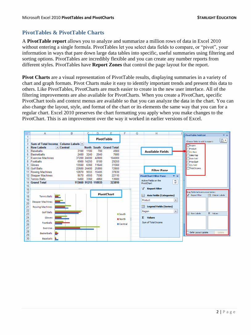
PivotTables & PivotTable Charts

A PivotTable report allows you to analyze and summarize a million rows of data in Excel 2010

without entering a single formula. PivotTables let you select data fields to compare, or “pivot”, your

information in ways that pare down large data tables into specific, useful summaries using filtering and

sorting options. PivotTables are incredibly flexible and you can create any number reports from

different styles. PivotTables have Report Zones that control the page layout for the report.

Pivot Charts are a visual representation of PivotTable results, displaying summaries in a variety of

chart and graph formats. Pivot Charts make it easy to identify important trends and present this data to

others. Like PivotTables, PivotCharts are much easier to create in the new user interface. All of the

filtering improvements are also available for PivotCharts. When you create a PivotChart, specific

PivotChart tools and context menus are available so that you can analyze the data in the chart. You can

also change the layout, style, and format of the chart or its elements the same way that you can for a

regular chart. Excel 2010 preserves the chart formatting you apply when you make changes to the

PivotChart. This is an improvement over the way it worked in earlier versions of Excel.

PivotTable

Available Fields

Filter Pane

PivotChart


3 | P a g e

Creating a PivotTable

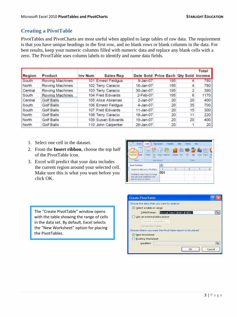
PivotTables and PivotCharts are most useful when applied to large tables of raw data. The requirement

is that you have unique headings in the first row, and no blank rows or blank columns in the data. For

best results, keep your numeric columns filled with numeric data and replace any blank cells with a

zero. The PivotTable uses column labels to identify and name data fields.

1. Select one cell in the dataset.

2. From the Insert ribbon, choose the top half

of the PivotTable icon.

3. Excel will predict that your data includes

the current region around your selected cell.

Make sure this is what you want before you

click OK.

The “Create PivotTable” window opens with the table showing the range of cells in the data set. By default, Excel selects the “New Worksheet” option for placing the PivotTables.


4 | P a g e

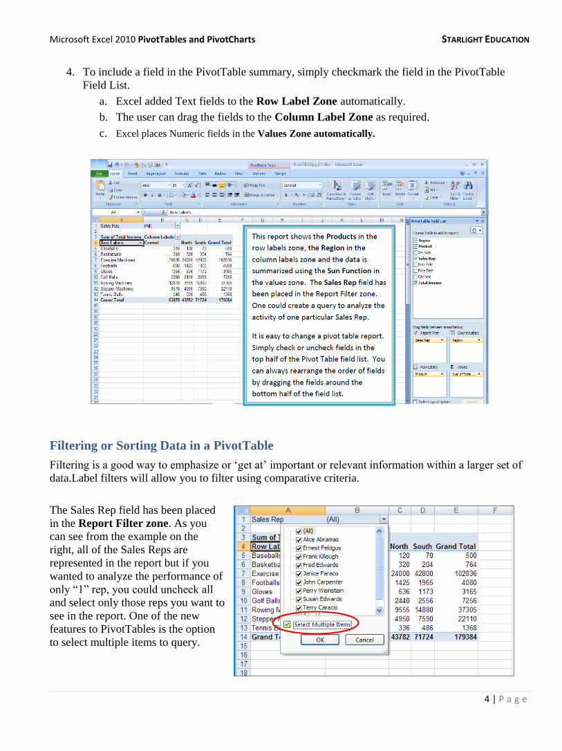
4. To include a field in the PivotTable summary, simply checkmark the field in the PivotTable

Field List.

a. Excel added Text fields to the Row Label Zone automatically.

b. The user can drag the fields to the Column Label Zone as required.

c. Excel places Numeric fields in the Values Zone automatically.

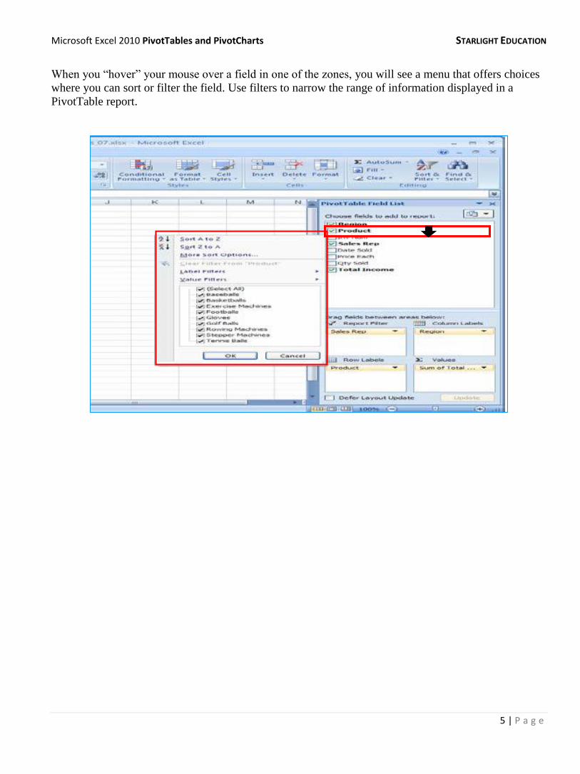
Filtering or Sorting Data in a PivotTable

Filtering is a good way to emphasize or ‘get at’ important or relevant information within a larger set of

data.Label filters will allow you to filter using comparative criteria.

The Sales Rep field has been placed

in the Report Filter zone. As you

can see from the example on the

right, all of the Sales Reps are

represented in the report but if you

wanted to analyze the performance of

only “1” rep, you could uncheck all

and select only those reps you want to

see in the report. One of the new

features to PivotTables is the option

to select multiple items to query.


5 | P a g e

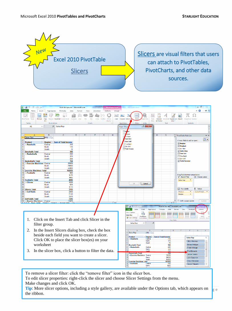
When you “hover” your mouse over a field in one of the zones, you will see a menu that offers choices

where you can sort or filter the field. Use filters to narrow the range of information displayed in a

PivotTable report.


6 | P a g e

Excel 2010 PivotTable

Slicers

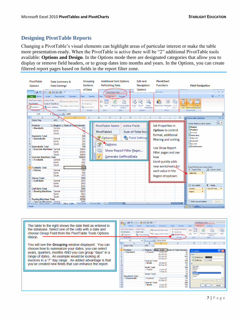
Slicers are visual filters that users

can attach to PivotTables,

PivotCharts, and other data

sources.

1. Click on the Insert Tab and click Slicer in the

filter group.

2. In the Insert Slicers dialog box, check the box

beside each field you want to create a slicer.

Click OK to place the slicer box(es) on your

worksheet

3. In the slicer box, click a button to filter the data.

To remove a slicer filter: click the “remove filter” icon in the slicer box.

To edit slicer properties: right-click the slicer and choose Slicer Settings from the menu.

Make changes and click OK.

Tip: More slicer options, including a style gallery, are available under the Options tab, which appears on

the ribbon.


7 | P a g e

Designing PivotTable Reports

Changing a PivotTable’s visual elements can highlight areas of particular interest or make the table

more presentation-ready. When the PivotTable is active there will be “2” additional PivotTable tools

available: Options and Design. In the Options mode there are designated categories that allow you to

display or remove field headers, or to group dates into months and years. In the Options, you can create

filtered report pages based on fields in the report filter zone.


8 | P a g e

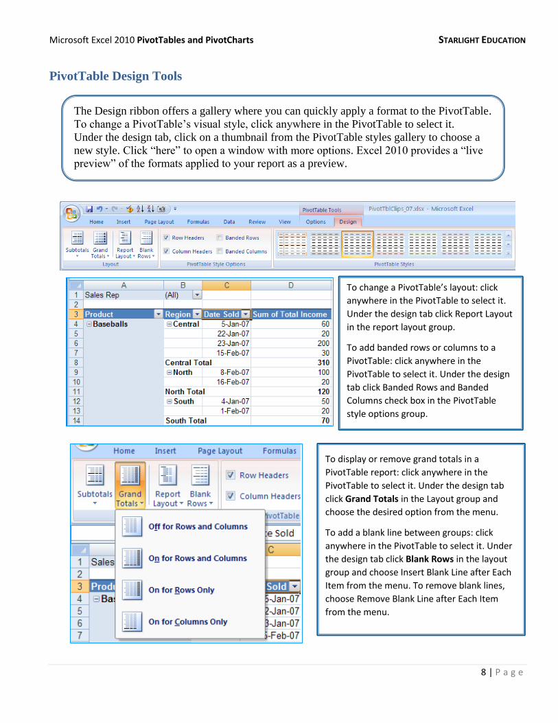
PivotTable Design Tools

The Design ribbon offers a gallery where you can quickly apply a format to the PivotTable.

To change a PivotTable’s visual style, click anywhere in the PivotTable to select it.

Under the design tab, click on a thumbnail from the PivotTable styles gallery to choose a

new style. Click “here” to open a window with more options. Excel 2010 provides a “live

preview” of the formats applied to your report as a preview.

To change a PivotTable’s layout: click

anywhere in the PivotTable to select it.

Under the design tab click Report Layout

in the report layout group.

To add banded rows or columns to a

PivotTable: click anywhere in the

PivotTable to select it. Under the design

tab click Banded Rows and Banded

Columns check box in the PivotTable

style options group.

To display or remove grand totals in a

PivotTable report: click anywhere in the

PivotTable to select it. Under the design tab

click Grand Totals in the Layout group and

choose the desired option from the menu.

To add a blank line between groups: click

anywhere in the PivotTable to select it. Under

the design tab click Blank Rows in the layout

group and choose Insert Blank Line after Each

Item from the menu. To remove blank lines,

choose Remove Blank Line after Each Item

from the menu.


9 | P a g e

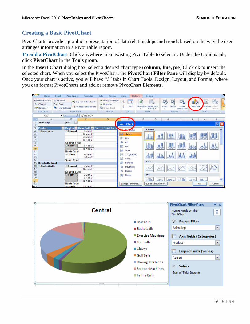
Creating a Basic PivotChart

PivotCharts provide a graphic representation of data relationships and trends based on the way the user

arranges information in a PivotTable report.

To add a PivotChart: Click anywhere in an existing PivotTable to select it. Under the Options tab,

click PivotChart in the Tools group.

In the Insert Chart dialog box, select a desired chart type (column, line, pie).Click ok to insert the

selected chart. When you select the PivotChart, the PivotChart Filter Pane will display by default.

Once your chart is active, you will have “3” tabs in Chart Tools; Design, Layout, and Format, where

you can format PivotCharts and add or remove PivotChart Elements.


10 | P a g e

Appendix

Quick Reference Guide

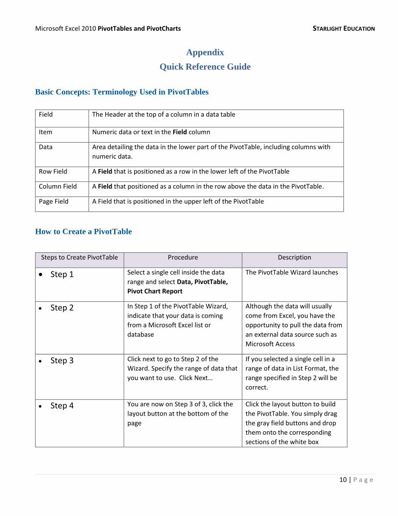
Basic Concepts: Terminology Used in PivotTables

Field The Header at the top of a column in a data table

Item Numeric data or text in the Field column

Data Area detailing the data in the lower part of the PivotTable, including columns with

numeric data.

Row Field A Field that is positioned as a row in the lower left of the PivotTable

Column Field A Field that positioned as a column in the row above the data in the PivotTable.

Page Field A Field that is positioned in the upper left of the PivotTable

How to Create a PivotTable

Steps to Create PivotTable Procedure Description

Step 1 Select a single cell inside the data

range and select Data, PivotTable,

Pivot Chart Report

The PivotTable Wizard launches

Step 2 In Step 1 of the PivotTable Wizard,

indicate that your data is coming

from a Microsoft Excel list or

database

Although the data will usually

come from Excel, you have the

opportunity to pull the data from

an external data source such as

Microsoft Access

Step 3 Click next to go to Step 2 of the

Wizard. Specify the range of data that

you want to use. Click Next…

If you selected a single cell in a

range of data in List Format, the

range specified in Step 2 will be

correct.

Step 4 You are now on Step 3 of 3, click the

layout button at the bottom of the

page

Click the layout button to build

the PivotTable. You simply drag

the gray field buttons and drop

them onto the corresponding

sections of the white box


11 | P a g e

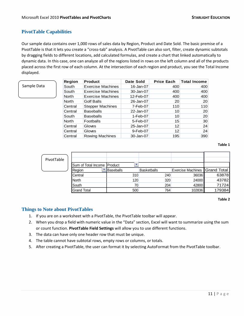
PivotTable Capabilities

Our sample data contains over 1,000 rows of sales data by Region, Product and Date Sold. The basic premise of a

PivotTable is that it lets you create a “cross-tab” analysis. A PivotTable can also sort, filter, create dynamic subtotals

by dragging fields to different locations, add calculated formulas, and create a chart that linked automatically to

dynamic data. In this case, one can analyze all of the regions listed in rows on the left column and all of the products

placed across the first row of each column. At the intersection of each region and product, you see the Total Income

displayed.

Region Product Date Sold Price Each Total Income

South Exercise Machines 16-Jan-07 400 400

South Exercise Machines 30-Jan-07 400 400

North Exercise Machines 12-Feb-07 400 400

North Golf Balls 26-Jan-07 20 20

Central Stepper Machines 7-Feb-07 110 110

Central Baseballs 22-Jan-07 10 20

South Baseballs 1-Feb-07 10 20

North Footballs 5-Feb-07 15 30

Central Gloves 25-Jan-07 12 24

Central Gloves 9-Feb-07 12 24

Central Rowing Machines 30-Jan-07 195 390

Table 1

Sum of Total Income Product

Region Baseballs Basketballs Exercise Machines

Central 310 240 36036

North 120 320 24000

South 70 204 42800

Grand Total 500 764 102836

Grand Total

63878

43782

71724

179384

Table 2

Things to Note about PivotTables

1. If you are on a worksheet with a PivotTable, the PivotTable toolbar will appear.

2. When you drop a field with numeric value in the “Data” section, Excel will want to summarize using the sum

or count function. PivotTable Field Settings will allow you to use different functions.

3. The data can have only one header row that must be unique.

4. The table cannot have subtotal rows, empty rows or columns, or totals.

5. After creating a PivotTable, the user can format it by selecting AutoFormat from the PivotTable toolbar.

Sample Data

PivotTable


12 | P a g e

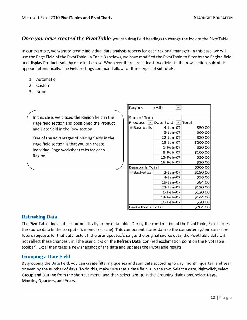
Once you have created the PivotTable, you can drag field headings to change the look of the PivotTable.

In our example, we want to create individual data analysis reports for each regional manager. In this case, we will

use the Page Field of the PivotTable. In Table 3 (below), we have modified the PivotTable to filter by the Region field

and display Products sold by date in the row. Whenever there are at least two fields in the row section, subtotals

appear automatically. The Field settings command allow for three types of subtotals:

1. Automatic

2. Custom

3. None

Region (All)

Sum of Total Income

Product Date Sold Total

Baseballs 4-Jan-07 $50.00

5-Jan-07 $60.00

22-Jan-07 $20.00

23-Jan-07 $200.00

1-Feb-07 $20.00

8-Feb-07 $100.00

15-Feb-07 $30.00

16-Feb-07 $20.00

Baseballs Total $500.00

Basketballs 2-Jan-07 $180.00

4-Jan-07 $96.00

19-Jan-07 $84.00

22-Jan-07 $120.00

6-Feb-07 $120.00

14-Feb-07 $144.00

16-Feb-07 $20.00

Basketballs Total $764.00

Refreshing Data

The PivotTable does not link automatically to the data table. During the construction of the PivotTable, Excel stores

the source data in the computer’s memory (cache). This component stores data so the computer system can serve

future requests for that data faster. If the user updates/changes the original source data, the PivotTable data will

not reflect these changes until the user clicks on the Refresh Data icon (red exclamation point on the PivotTable

toolbar). Excel then takes a new snapshot of the data and updates the PivotTable results.

Grouping a Date Field

By grouping the Date field, you can create filtering queries and sum data according to day, month, quarter, and year

or even by the number of days. To do this, make sure that a date field is in the row. Select a date, right-click, select

Group and Outline from the shortcut menu, and then select Group. In the Grouping dialog box, select Days,

Months, Quarters, and Years.

In this case, we placed the Region field in the

Page field section and positioned the Product

and Date Sold in the Row section.

One of the advantages of placing fields in the

Page field section is that you can create

individual Page worksheet tabs for each

Region.


13 | P a g e

Sorting Items

You can sort PivotTable items according to a selected field, according to Excel’s sorting rules. Select an item in the

Row field. Click the Sort Ascending or Sort Descending icon, or from the Data menu, select Sort.

Inserting a Calculated Field

Calculated fields are fields with formulas. The dynamic formulas you insert into the PivotTable will allow you to

perform calculations between fields or in a single field.

1. Select one of the cells in the data area of the PivotTable.

2. On the PivotTable toolbar, select PivotTable, Formulas, Calculated Field.

3. In the Name box, type the name of the formula. This name will be the name of the calculated field and Excel

will save the formula with the new field name.

4. In the Fields box, select the value field, which will be part of the formula…

Example: Create a formula named Discount. In the formula field, type =Total Income * . 02

In the PivotTable, the Discount field would appear to the right of the Total Income column.

Inserting Fields to Calculate % and More

Insert various additional calculated fields by using the Options button in the PivotTable Fields dialog box. You can

choose to view the Show data as options:

Regular

Difference From

% Of

% Difference From

Running Total In

% of Row

% of Column

% of Total

Index


14 | P a g e

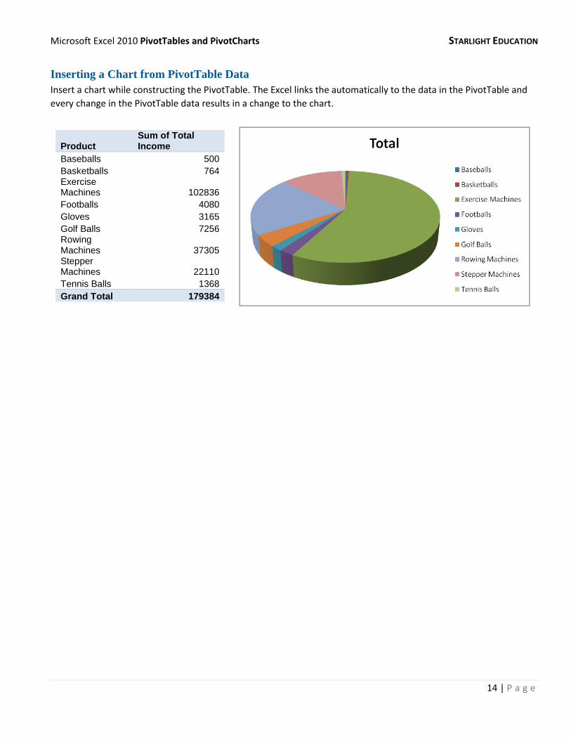
Inserting a Chart from PivotTable Data

Insert a chart while constructing the PivotTable. The Excel links the automatically to the data in the PivotTable and

every change in the PivotTable data results in a change to the chart.

Product Sum of Total Income

Baseballs 500

Basketballs 764 Exercise Machines 102836

Footballs 4080

Gloves 3165

Golf Balls 7256 Rowing Machines 37305 Stepper Machines 22110

Tennis Balls 1368

Grand Total 179384

Documents

PivotTables and PivotChartsstarlighteducation.com/files/Excel 2010 PivotTables_PivotCharts Ref... · Microsoft Excel 2010 SPivotTables and PivotCharts TARLIGHT EDUCATION 3 | P a g