Easily Master Microsoft® Excel® PivotTables

N A M E

E V E N T N U M B E R / D A T E

800-556-2998

pryor.com

SEMINAR WORKBOOK

Easily Master Microsoft® Excel® PivotTables

Microsoft, Windows, Excel, Access, Project, SharePoint, OneDrive, Word, PowerPoint, and Visio are all registered trademarks of Microsoft Corporation.

DISCLAIMER: The principles and suggestions in this workbook and seminar are presented to apply to diverse personal and company situations. These materials and the overall seminar are for general informational and educational purposes only. The materials and the seminar, in general, are presented with the understanding that Pryor Learning is not engaged in rendering legal advice. You should always consult an attorney with any legal issues.

©2020 Pryor Learning, Inc. Registered U.S. Patent & Trademark Office and Canadian Trade-Marks office. Except for the inclusion of brief quotations in a review, no part of this book may be reproduced or utilized in any form or by any means, electronic or mechanical, including photocopying, recording or by any information storage and retrieval system, without permission in writing from Pryor Learning, Inc.

https://www.pryor.com

©Pryor Learning, Inc. • WE32007ES-DL

1

1. What Is a PivotTable? . . . . . . . . . . . . . . . . . . . . . . . . . . . . .1

2. Prepare the Worksheet Data . . . . . . . . . . . . . . . . . . . . . .1

3. Insert a PivotTable . . . . . . . . . . . . . . . . . . . . . . . . . . . . . . . .1

4. Change the Design of the PivotTable . . . . . . . . . . . . . .3

5. Analyze the Data . . . . . . . . . . . . . . . . . . . . . . . . . . . . . . . . .4

6. Add a PivotChart to the PivotTable . . . . . . . . . . . . . . . .9

Appendix . . . . . . . . . . . . . . . . . . . . . . . . . . . . . . . . . . . . . . . . . 15

Table of Contents

i

©Pryor Learning, Inc. • WE32007ES-DL 1

What Is a PivotTable?Analyzing raw data can, at the best of times, turn into a nightmare if you have to deal with hundreds and thousands of records . Excel offers a powerful data analysis tool, called a PivotTable .

A PivotTable enables you to analyze complex data or large data sets into a summarized report . Once you create the PivotTable, you can then pivot the data, edit it, format it, perform calculations etc .

By creating a PivotTable report, you are able to view:

• a breakdown of customers by sales, or customers by product, or sales by city and so on

• a breakdown of sales by year, month, days or quarters

• perform calculations such as Sum, Average, Count

• perform custom calculations

• a combination of all of the above

Prepare the Worksheet DataBefore you create a PivotTable, here are some things to consider about the data source:

• Do not include blank columns/rows in the data .

• Avoid blank cells with no values; use a zero value instead of a blank .

• Avoid the temptation to merge cells, especially on the header rows .

• Remove total rows .

• Unhide any hidden columns/rows .

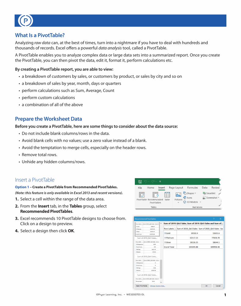
Insert a PivotTableOption 1 – Create a PivotTable from Recommended PivotTables.

(Note: this feature is only available in Excel 2013 and recent versions).

1. Select a cell within the range of the data area .

2. From the Insert tab, in the Tables group, selectRecommended PivotTables .

3. Excel recommends 10 PivotTable designs to choose from . Click on a design to preview .

4. Select a design then click OK .

©Pryor Learning, Inc. • WE32007ES-DL2

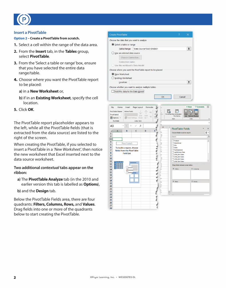
Insert a PivotTableOption 2 – Create a PivotTable from scratch.

1. Select a cell within the range of the data area .

2. From the Insert tab, in the Tables group,select PivotTable .

3. From the ‘Select a table or range’ box, ensurethat you have selected the entire datarange/table .

4. Choose where you want the PivotTable reportto be placed:

a) in a New Worksheet or,

b) if in an Existing Worksheet, specify the celllocation .

5. Click OK .

The PivotTable report placeholder appears to the left, while all the PivotTable fields (that is extracted from the data source) are listed to the right of the screen .

When creating the PivotTable, if you selected to insert a PivotTable in a ‘New Worksheet’, then notice the new worksheet that Excel inserted next to the data source worksheet .

Two additional contextual tabs appear on the ribbon:

a) The PivotTable Analyze tab (in the 2010 andearlier version this tab is labelled as Options),

b) and the Design tab .

Below the PivotTable Fields area, there are four quadrants: Filters, Columns, Rows, and Values . Drag fields into one or more of the quadrants below to start creating the PivotTable .


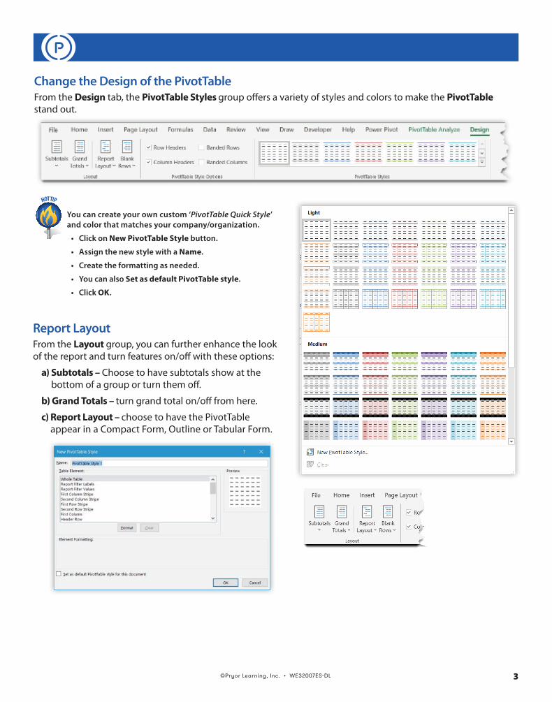
Change the Design of the PivotTableFrom the Design tab, the PivotTable Styles group offers a variety of styles and colors to make the PivotTable stand out .

You can create your own custom ‘PivotTable Quick Style’ and color that matches your company/organization.

• Click on New PivotTable Style button.

• Assign the new style with a Name.

• Create the formatting as needed.

• You can also Set as default PivotTable style.

• Click OK.

Report LayoutFrom the Layout group, you can further enhance the look of the report and turn features on/off with these options:

a) Subtotals – Choose to have subtotals show at thebottom of a group or turn them off .

b) Grand Totals – turn grand total on/off from here .

c) Report Layout – choose to have the PivotTableappear in a Compact Form, Outline or Tabular Form .


Analyze the Data

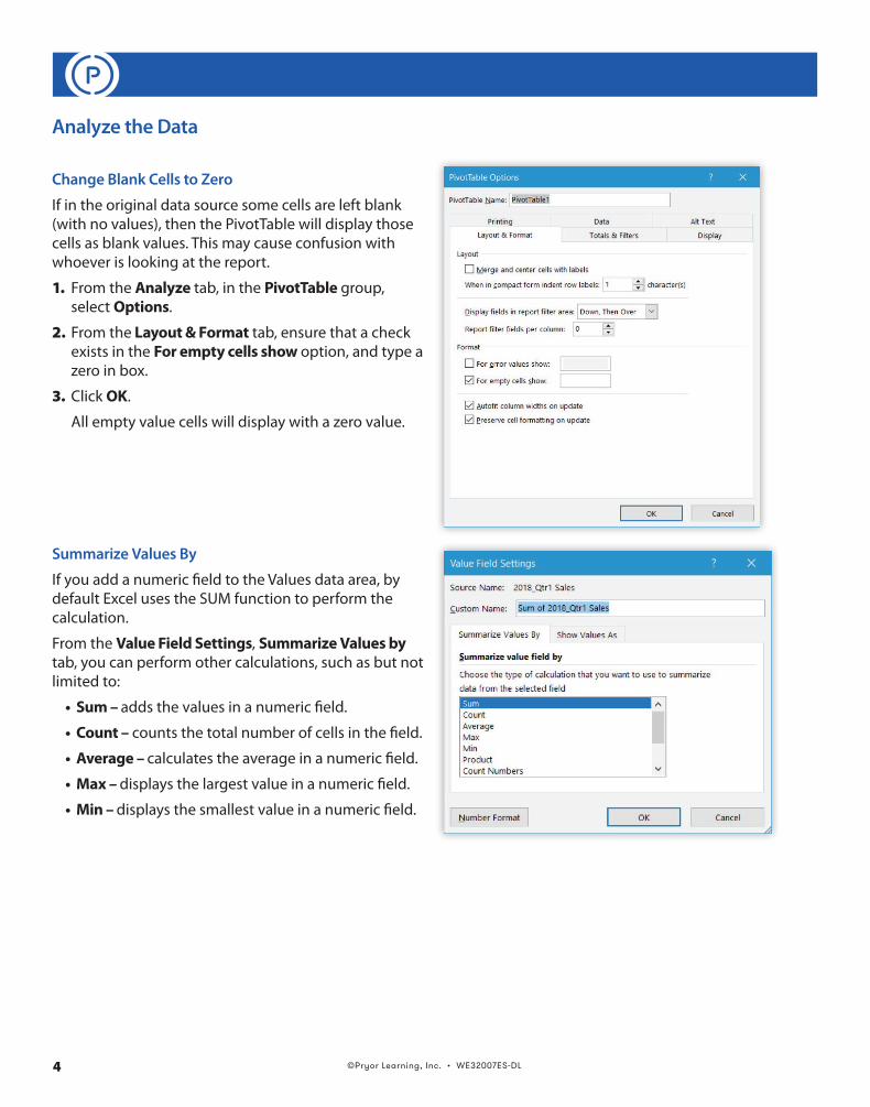
Change Blank Cells to Zero

If in the original data source some cells are left blank (with no values), then the PivotTable will display those cells as blank values . This may cause confusion with whoever is looking at the report .

1. From the Analyze tab, in the PivotTable group,select Options .

2. From the Layout & Format tab, ensure that a checkexists in the For empty cells show option, and type azero in box .

3. Click OK .

All empty value cells will display with a zero value .

Summarize Values By

If you add a numeric field to the Values data area, by default Excel uses the SUM function to perform the calculation .

From the Value Field Settings, Summarize Values by tab, you can perform other calculations, such as but not limited to:

• Sum – adds the values in a numeric field .

• Count – counts the total number of cells in the field .

• Average – calculates the average in a numeric field .

• Max – displays the largest value in a numeric field .

• Min – displays the smallest value in a numeric field .


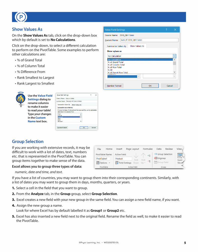
Show Values AsOn the Show Values As tab, click on the drop-down box which by default is set to No Calculations .

Click on the drop-down, to select a different calculation to perform on the PivotTable . Some examples to perform other calculations are:

• % of Grand Total

• % of Column Total

• % Difference From

• Rank Smallest to Largest

• Rank Largest to Smallest

Group SelectionIf you are working with extensive records, it may be difficult to work with a lot of dates, text, numbers etc . that is represented in the PivotTable . You can group items together to make sense of the data .

Excel allows you to group three types of data:

numeric, date and time, and text.

If you have a list of countries, you may want to group them into their corresponding continents . Similarly, with a list of dates you may want to group them in days, months, quarters, or years .

1. Select a cell in the field that you want to group .

2. From the Analyze tab, in the Group group, select Group Selection .

3. Excel creates a new field with your new group in the same field . You can assign a new field name, if you want .

4. Assign the new group a name . Look for where Excel has by default labelled it as Group1 or Group2 etc .

5. Excel has also inserted a new field next to the original field . Rename the field as well, to make it easier to readthe PivotTable .

Use the Value Field Settings dialog to rename columns to make it easier to read your table! Type your changes in the Custom Name text box.


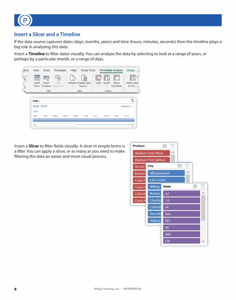
Insert a Slicer and a TimelineIf the data source captures dates (days, months, years) and time (hours, minutes, seconds) then the timeline plays a big role in analyzing this data .

Insert a Timeline to filter dates visually . You can analyze the data by selecting to look at a range of years, or perhaps by a particular month, or a range of days .

Insert a Slicer to filter fields visually . A slicer in simple terms is a filter . You can apply a slicer, or as many as you need to make filtering the data an easier and more visual process .


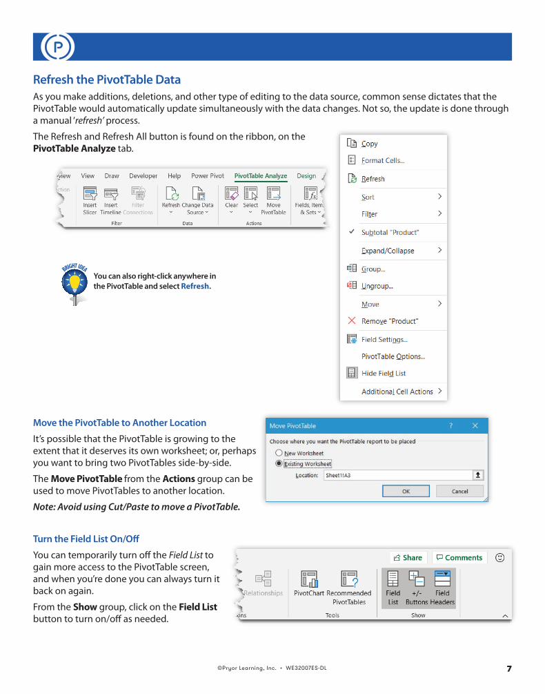
Refresh the PivotTable DataAs you make additions, deletions, and other type of editing to the data source, common sense dictates that the PivotTable would automatically update simultaneously with the data changes . Not so, the update is done through a manual ‘refresh’ process .

The Refresh and Refresh All button is found on the ribbon, on the PivotTable Analyze tab .

Move the PivotTable to Another Location

It’s possible that the PivotTable is growing to the extent that it deserves its own worksheet; or, perhaps you want to bring two PivotTables side-by-side .

The Move PivotTable from the Actions group can be used to move PivotTables to another location .

Note: Avoid using Cut/Paste to move a PivotTable.

Turn the Field List On/Off

You can temporarily turn off the Field List to gain more access to the PivotTable screen, and when you’re done you can always turn it back on again .

From the Show group, click on the Field List button to turn on/off as needed .

You can also right-click anywhere in the PivotTable and select Refresh.

ADVANCED USER

BRIGHT IDEAHOT TIP


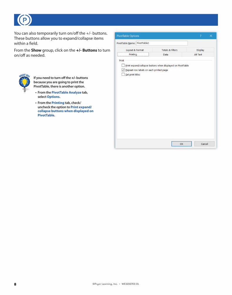
You can also temporarily turn on/off the +/- buttons . These buttons allow you to expand/collapse items within a field .

From the Show group, click on the +/- Buttons to turn on/off as needed .

If you need to turn off the +/- buttons because you are going to print the PivotTable, there is another option.

• From the PivotTable Analyze tab,select Options.

• From the Printing tab, check/uncheck the option to Print expand/collapse buttons when displayed on PivotTable.

ADVANCEDUSER

BRIGHT IDEAHOT TIP


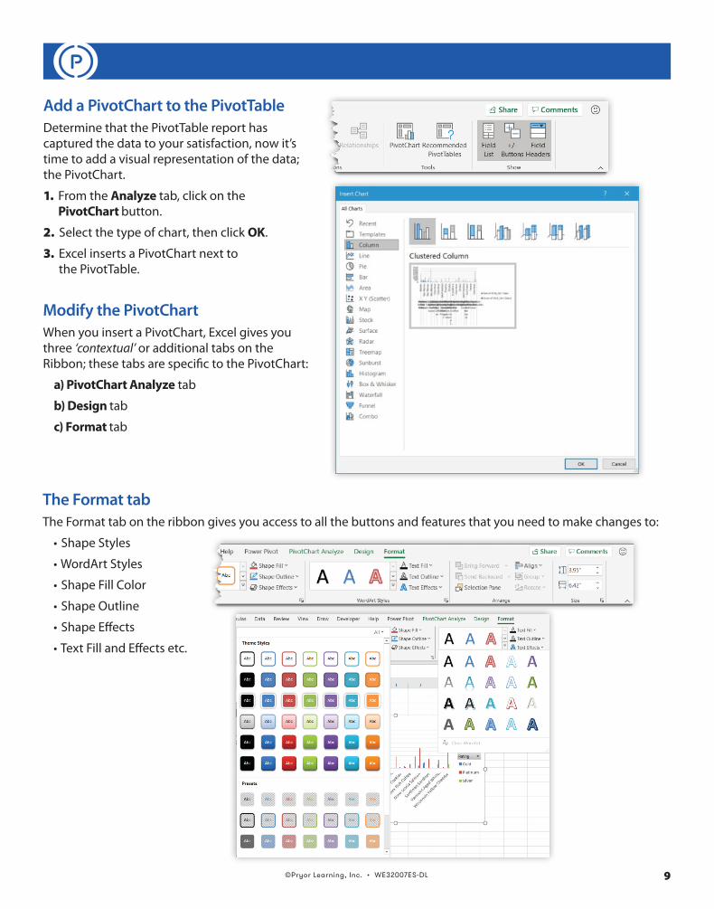
Add a PivotChart to the PivotTableDetermine that the PivotTable report has captured the data to your satisfaction, now it’s time to add a visual representation of the data; the PivotChart .

1. From the Analyze tab, click on thePivotChart button .

2. Select the type of chart, then click OK .

3. Excel inserts a PivotChart next tothe PivotTable .

The Format tabThe Format tab on the ribbon gives you access to all the buttons and features that you need to make changes to:

• Shape Styles

• WordArt Styles

• Shape Fill Color

• Shape Outline

• Shape Effects

• Text Fill and Effects etc .

Modify the PivotChartWhen you insert a PivotChart, Excel gives you three ‘contextual’ or additional tabs on the Ribbon; these tabs are specific to the PivotChart:

a) PivotChart Analyze tab

b) Design tab

c) Format tab


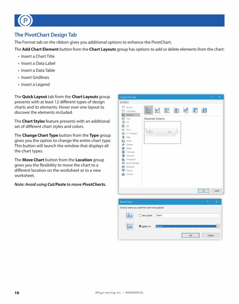
The PivotChart Design TabThe Format tab on the ribbon gives you additional options to enhance the PivotChart .

The Add Chart Element button from the Chart Layouts group has options to add or delete elements from the chart:

• Insert a Chart Title

• Insert a Data Label

• Insert a Data Table

• Insert Gridlines

• Insert a Legend

The Quick Layout tab from the Chart Layouts group presents with at least 12 different types of design charts and its elements . Hover over one layout to discover the elements included .

The Chart Styles feature presents with an additional set of different chart styles and colors .

The Change Chart Type button from the Type group gives you the option to change the entire chart type . This button will launch the window that displays all the chart types .

The Move Chart button from the Location group gives you the flexibility to move the chart to a different location on the worksheet or to a new worksheet .

Note: Avoid using Cut/Paste to move PivotCharts.


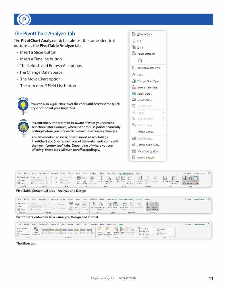
The PivotChart Analyze TabThe PivotChart Analyze tab has almost the same identical buttons as the PivotTable Analyze tab .

• Insert a Slicer button

• Insert a Timeline button

• The Refresh and Refresh All options

• The Change Data Source

• The Move Chart option

• The turn on/off Field List button

It’s extremely important to be aware of what your current selection is (for example, where is the mouse pointer currently resting) before you proceed to make the necessary changes.

You have looked at so far, how to insert a PivotTable, a PivotChart and Slicers. Each one of these elements come with their own ‘contextual’ tabs. Depending of where you are ‘clicking’ these tabs will turn on/off accordingly.

You can also ‘right-click’ over the chart and access some quick style options at your fingertips.

PivotTable Contextual tabs – Analyze and Design

PivotChart Contextual tabs – Analyze, Design and Format

The Slicer tab

ADVANCED USER

BRIGHT IDEAHOT TIP


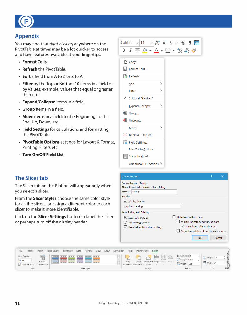
AppendixYou may find that right-clicking anywhere on the PivotTable at times may be a lot quicker to access and have features available at your fingertips .

• Format Cells .

• Refresh the PivotTable .

• Sort a field from A to Z or Z to A .

• Filter by the Top or Bottom 10 items in a field or by Values; example, values that equal or greater than etc .

• Expand/Collapse items in a field .

• Group items in a field .

• Move items in a field; to the Beginning, to the End, Up, Down, etc .

• Field Settings for calculations and formatting the PivotTable .

• PivotTable Options settings for Layout & Format, Printing, Filters etc .

• Turn On/Off Field List .

The Slicer tabThe Slicer tab on the Ribbon will appear only when you select a slicer .

From the Slicer Styles choose the same color style for all the slicers, or assign a different color to each slicer to make it more identifiable .

Click on the Slicer Settings button to label the slicer or perhaps turn off the display header .


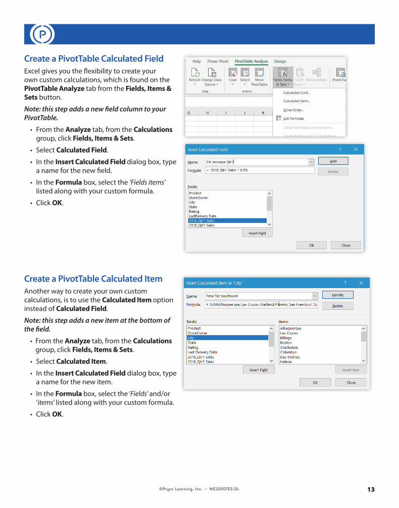
Create a PivotTable Calculated FieldExcel gives you the flexibility to create your own custom calculations, which is found on the PivotTable Analyze tab from the Fields, Items & Sets button .

Note: this step adds a new field column to your PivotTable.

• From the Analyze tab, from the Calculationsgroup, click Fields, Items & Sets .

• Select Calculated Field .

• In the Insert Calculated Field dialog box, typea name for the new field .

• In the Formula box, select the ‘Fields items’listed along with your custom formula .

• Click OK .

Create a PivotTable Calculated ItemAnother way to create your own custom calculations, is to use the Calculated Item option instead of Calculated Field .

Note: this step adds a new item at the bottom of the field.

• From the Analyze tab, from the Calculationsgroup, click Fields, Items & Sets .

• Select Calculated Item .

• In the Insert Calculated Field dialog box, typea name for the new item .

• In the Formula box, select the ‘Fields’ and/or‘items’ listed along with your custom formula .

• Click OK .


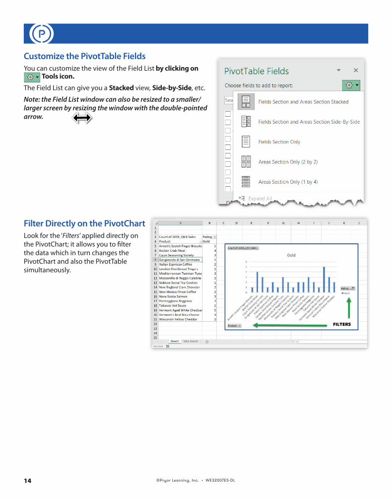
Customize the PivotTable FieldsYou can customize the view of the Field List by clicking on

Tools icon.

The Field List can give you a Stacked view, Side-by-Side, etc .

Note: the Field List window can also be resized to a smaller/larger screen by resizing the window with the double-pointed arrow.

Filter Directly on the PivotChartLook for the ‘Filters’ applied directly on the PivotChart; it allows you to filter the data which in turn changes the PivotChart and also the PivotTable simultaneously .


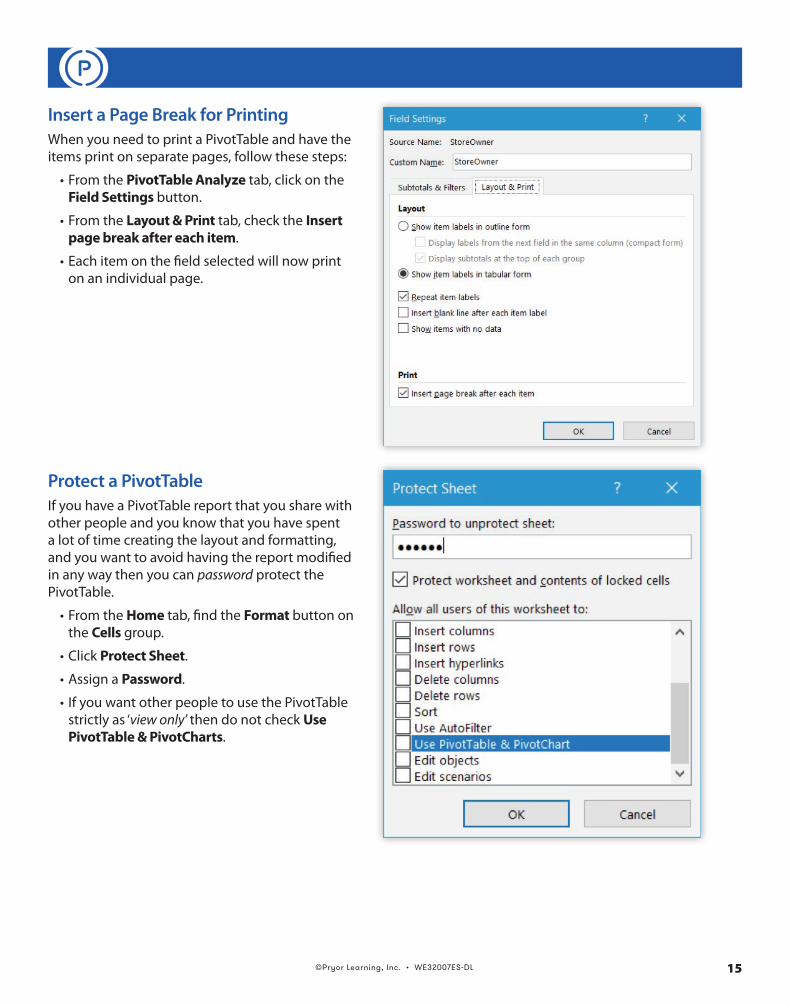
Insert a Page Break for PrintingWhen you need to print a PivotTable and have the items print on separate pages, follow these steps:

• From the PivotTable Analyze tab, click on theField Settings button .

• From the Layout & Print tab, check the Insertpage break after each item .

• Each item on the field selected will now printon an individual page .

Protect a PivotTableIf you have a PivotTable report that you share with other people and you know that you have spent a lot of time creating the layout and formatting, and you want to avoid having the report modified in any way then you can password protect the PivotTable .

• From the Home tab, find the Format button onthe Cells group .

• Click Protect Sheet .

• Assign a Password .

• If you want other people to use the PivotTablestrictly as ‘view only’ then do not check UsePivotTable & PivotCharts .

Documents

Easily Master Microsoft® Excel® PivotTables