Evaluation of three pollutant dispersion models for the ... · The AERMOD model is a linear steady-state plume model. The formulations of the AERMOD program are grounded along the

Global NEST Journal, Vol 19, No 1, pp 37-48 Copyright© 2017 Global NEST

Printed in Greece. All rights reserved

Demirarslan K.O., Çetin Doğruparmak Ş. and Karademir A. (2017), Evaluation of three pollutant dispersion models for the environmental

assessment of a district in Kocaeli, Turkey, Global NEST Journal, 19(1), 37-48.

Evaluation of three pollutant dispersion models for the environmental assessment of a district in Kocaeli, Turkey

Demirarslan K.O.1,*, Çetin Doğruparmak Ş.2 and Karademir A.3

1Department of Environmental Engineering, Artvin Çoruh University 08000 Artvin, Turkey 2Department of Environmental Engineering, Kocaeli University, 41380 Kocaeli, Turkey

3Department of Environmental Engineering, Kocaeli University, 41380 Kocaeli, Turkey

Received: 21/01/2016, Accepted: 18/12/2016, Available online: 15/02/2017

*to whom all correspondence should be addressed:

e-mail: [email protected]

Abstract

Air Quality Modeling is a method used to manage urban air quality. Various pollutant dispersion models are available, and each of these models is characterized by its own advantages and disadvantages. Thus, we aimed to evaluate the advantages and disadvantages of the models and to determine their performance by applying them to a specific district. This study also enabled the determination of the contribution of pollution sources to the total pollution and the current air quality of the study area according to the selected pollutants. In this study, both steady-state models (the American Meteorological Society/Environmental Protection Agency Regulatory Model-AERMOD and the Industrial Source Complex Short Term Model-ISCST-3) and the Lagrangian model (the California Puff Model-CALPUFF) were used as the dispersion models. The Körfez district of Kocaeli was selected as the study area. SO2 and PM10 emissions were observed as pollutants. The statistical methods of mean squared error (MSE) and fractional bias (FB) were employed to evaluate the performance of these models.

The results of the study revealed that the highest concentration varied according to the models and time options. However, when the modeling results for all of the sources were examined, the highest concentration was calculated by ISCST-3. The effect of the line source was less than the other sources (point and area). The contributions of the pollution sources differed according to each modeling program. The results of the statistical methods, which were used for evaluating the performance of the models, varied according to both the pollutant type and the time option. An overall ranking regarding modeling performance is as follows: CALPUFF > AERMOD > ISCST-3 for PM10 and ISCST-3 > CALPUFF > AERMOD for SO2. The MSE/FB results demonstrated that the predicted values were lower than the measured outcomes. Similarly, a comparison of the predicted and measured values with national and international limits revealed that various measures are necessary to reduce SO2 and PM10.

Keywords: AERMOD, CALPUFF, ISCST-3, Körfez district, Pollutant dispersion modeling

1. Introduction

The aim of dispersion modeling is to evaluate the concentrations (at the receptor points) of pollutants released into the atmosphere from any source. A dispersion model represents mathematical or physical relationships, which are established on scientific principles for the concentrations of the released pollutants. Information regarding air quality in a study area can be derived from the modeling results. Modeling results can aid in selecting the location of a new factory and designing the chimney of the factory and can be used to determine the areas that are affected the most by the discharge source and to execute different scenarios in these areas (AQMG, 2010; Silva et al., 2013; Clappier et al., 2015).

Different methods are used to study pollutant dispersion. One method of modeling is the physical method in which the dispersion of pollutants is analyzed by recreating the environmental conditions in the laboratory. Another method involves mathematically modeling the pollutant dispersion (Markiewicz, 2008). Various scientific dispersion models are available, each of which is characterized by its own advantages and disadvantages.

Three different dispersion models, the American Meteorological Society/Environmental Protection Agency Regulatory Model (AERMOD VIEW 6.5.0), the Industrial Source Complex Short Term model (ISCST-3 6.5.0), and the California Puff Model (CALPUFF VIEW 5.8), were used to mathematically model the dispersion of pollutants. The Körfez district in Kocaeli was selected as the study area. SO2 and PM10 emissions were observed as the pollutants. The mean squared error (MSE) and fractional bias (FB) statistical methods were used to evaluate the performance of the selected models.

This study was important for two reasons. Firstly, by evaluating three different dispersion models rather than one, their advantages and disadvantages could be

mailto:[email protected]

38 DEMIRARSLAN et al.

determined. Statistical methods have been widely used in many recent studies. As the number of analysis methods used in any study increases, the accuracy of the obtained results is enhanced (Doğruparmak et al., 2014). Therefore, two different statistical methods were employed in order to evaluate the model performance. Another important point for this study was the evaluation of air quality in the Körfez district, considering the SO2 and PM10 pollutants. Due to the presence of industrial activities, urbanization, ports, docks, railroads and highways, this is one of the most heavily polluted districts in the Kocaeli Province in terms of air quality (Civan and Kara, 2016). Determining the air pollutants, and interpreting and examining their environmental effects will lead to future planning studies. These studies will help predict the future adverse effects and develop measures for adoption. This development is an important step for “Clean Air Action Plans”.

2. Materials and Methods

2.1. Study Area

The Körfez district is located on the west coast of the Kocaeli Province, in the Marmara Region of Turkey. The land area of the district is 398 km2, and the total population of the district was 130,730 in 2009. There are 15 villages, 11 districts and 865 streets and alleys within the boundaries of the district, and there are 14,150 buildings and 29,128 residential homes in the district center. In addition, 3864 workplaces, including industry organizations, are situated in the district. The construction areas and the green areas constitute 60% and 40% of the total study area, respectively. This district is a hub not only for industry but also for ports and piers. Due to the railway, the D-100 highway and the TEM motorway, this district represents a heavily trafficked transition point between Europe, Asia, and the Middle East (Korfez District). A satellite image of the study area is shown in Figure 1.

Figure 1. Satellite image of the study area

2.2. Modeling Methodology

The AERMOD model is a linear steady-state plume model. The formulations of the AERMOD program are grounded along the atmospheric turbulence. As of November 9, 2006, this program was replaced with the ISCST-3 program for near-range forecasts (up to 50 km from the source) and analyses (Mokhter et al., 2014). The AERMOD modeling program, which is a younger generation of the ISCST-3 program, includes a planetary boundary layer algorithm and improved land structure algorithms compared to the ISCST-3 program (Rood, 2014). The program can be applied to many different sources, including point, line, volume, and area sources.

The ISCST-3 model used in this study utilizes a steady-state Gaussian flow equation for high plume point sources (ISCST-3 Tech Guide, 2009). For a variety of pollution sources, the ISCST-3 model offers different options for modeling the dispersion of emissions that correspond to

the sources. This model is suitable for air quality estimates. The accuracy of the estimates depends on obtaining correct measurements of meteorological parameters in the study area and the elaboration and accuracy of emission inventories for all of the sources. The primary advantages of this model are that it is relatively simple to use and the meteorological data file required for the modeling is small compared to other dispersion models. However, data affecting the structure of the atmospheric boundary layer and the corresponding estimates of turbulence dispersion processes are not taken into consideration, which is a limitation of this model (Doğruparmak et al., 2009; Diaz and Zafrilla, 2012).

Gaussian plume models for predicting the downwind pollutant concentrations from point, line and area sources can be described as follows, (Wang et al., 2006)

Where C is the downwind pollutant concentration (g m-3), Qp is the point source pollutant emission rate (g s-1), QL is the line source pollutant emission rate (g m-1 s-1), QA is the

EVALUATION OF THREE POLLUTANT DISPERSION MODELS FOR THE ENVIRONMENTAL ASSESSMENT 39

area source pollutant emission rate (g m-2 s-1), y, z are the Pasquill–Gifford plume spread parameters based on stability class, u is the average wind speed at pollutant release height (m s-1), H is the effective height above ground of emission source (m), V is the vertical term used to describe the vertical distribution of the plume, x is the upwind direction (m), and y is the cross wind direction (m).

For point source

C= Qp

πσyσzu exp (-

y2

2σy2) exp (-

H2

2σz2)

(1)

For line source

C=2QL

√2πσzuexp (-

H2

2σz2) (2)

For area source

C= QA

2πu ∫

V

σyσz

(∫ exp [-1

2 (

y

σy

)

2

]Y

dy)X

dx (3)

CALPUFF is another program used for modeling the air quality of the area. CALPUFF is a Gaussian puff modeling program developed by the "Atmospheric Working Group" (Atmospheric Studies Group) and is used to estimate chemical transformations and the transportation of pollutants depending on varying meteorological conditions

of the region in unstable situations (Abdul-Wahab et al., 2014). This model has been accepted and recommended by the EPA for estimating the effect and long-distance transport of pollutants in meteorologically and geophysically complex cases (Rojas and Venegas, 2010; Macintosh et al., 2010; Cui et al., 2011). The basic equation for the contribution of a puff at a receptor is:

C=Q

2πσyσz

gexp (-da

2

2σx2) exp (-

dc2

2σy2) (4)

g= 2

(2π)1/2σz

∑ exp [ -(He+ 2nh)2/( 2σz2)]

∞

n=-∞

(5)

Where C is the ground-level concentration (g m-3), Q is the

pollutant mass (g) in the puff, x is the standard deviation (m) of the Gaussian distribution in the along-wind

direction, y is the standard deviation (m) of the Gaussian

distribution in the cross-wind direction, z is the standard deviation (m) of the Gaussian distribution in the vertical direction, da is the distance (m) from the puff center to the receptor in the along-wind direction, dc is the distance (m) from the puff center to the receptor in the cross-wind direction, g is the vertical term (m) of the Gaussian equation, H is the effective height (m) above ground of the puff center, and h is the mixed-layer height (m) (Jeong, 2011).

Table 1. Input data used in the dispersion model

Input Data Program

AERMOD ISCST-3 CALPUFF

Land use 40 % rural, 60 % urban 40 % rural, 60 % urban calculated by CALPUFF

In Rural Area;

50 % cultivated land, 50 % grassland

In Rural Area; 50 % cultivated land, 50 %

grassland calculated by CALPUFF

Receptors 1250 uniform cartesian

(50 x 25) 1250 uniform cartesian

(50 x 25) 1250 uniform cartesian

(50 x 25)

Grid size 740 m x740 m 740 m x740 m 740 m x740 m

Surface roughness length 0.62 0.62 calculated by CALPUFF

Albedo 0.2145 0.2145 calculated by CALPUFF

Bowen rate 1.89 1.89 calculated by CALPUFF

Distribution coefficient Urban Urban calculated by CALPUFF

Terrain coefficient Simple+complex Simple+complex calculated by CALPUFF

Time option 24h and annual 24h and annual 24h and annual

Map dwg extension dwg extension dwg extension

Meteorological data 2005-2009 hourly surface

and upper air met data 2005-2009 hourly surface

air met data 2005-2009 hourly surface

and upper air met data

Source data -Point sources -Area sources -Line sources

-Point sources -Area sources -Line sources

-Point sources -Area sources

The input data used for the dispersion models are summarized in Table 1.

The models in this study use annual data that are reported hourly as the meteorological data. The data used in the ISCST-3 are superficial hourly meteorological data. The AERMOD and CALPUFF models use the superficial meteorological data used for the ISCST-3 modeling

program and upper air meteorological data. In these models, meteorological data up to a maximum of 5 years can be used. Five-year data (2005-2009) have been used in the study because more meteorological data enhance the accuracy of the forecast (British Columbia Ministry of Environment, 2008). The hourly meteorological data


recorded by the “Lakes Environmental Software” were used in the models.

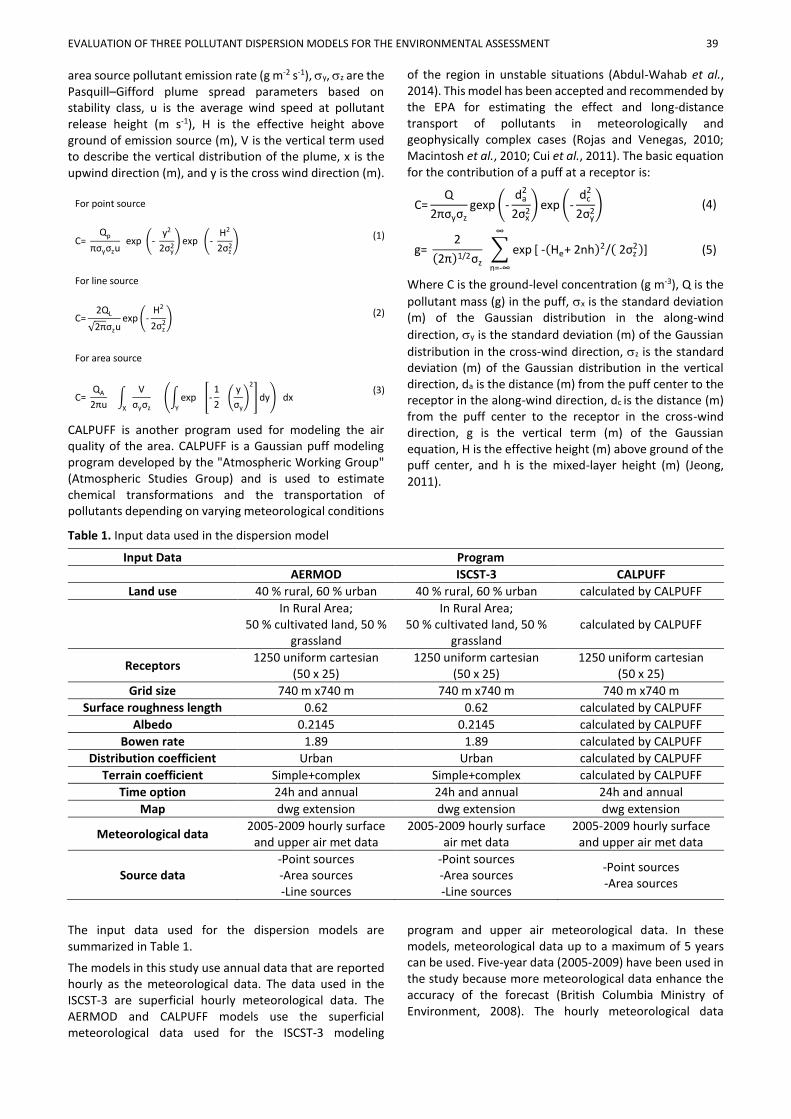
The data used in the ISCST-3 model include hourly temperature, wind velocity, wind direction, air pressure, cloud height, and precipitation measurements per day. The obtained meteorological data were processed using the RAMMET View program, which is a pre-processor of the ISCST-3 modeling program. Since the mixture heights were not evaluated in the meteorological stations, these data

were calculated using the pre-processor RAMMET View program. The wind data were processed using the WRLPLOT, which is also a processor of the ISCST-3 model. The wind rose data obtained by using this program for the years of 2005 to 2009 are shown in Figure 2.

The meteorological data used in CALPUFF and AERMOD were obtained using CALMET (a pre-processor of CALPUFF) and AERMET View (a pre-processor of AERMOD) modeling programs.

Figure 2. The wind rose prepared by WRLPLOT for data from 2005 to 2009

The point sources of SO2 and PM10 emissions were evaluated for 15 and 21 industrial plants, respectively, in the territorial district. The data related to the industrial plants and their emission rates were obtained from the Kocaeli Provincial Directorate of Environment and Urbanization. The data used comprise the number of factory chimneys, the factory chimney height (m), flue gas velocity (m s-1) and temperature (K), inner diameter of the chimney (m), and pollutant concentration (g s-1) (Emissions Report, 2009).

As the area sources, the residential areas of the district were evaluated. The residential areas were divided into 4 different regions because the construction areas constitute 60% and the green areas 40% of the total area. The approximate surface areas of residential regions 1, 2, 3 and 4 as calculated on the map were 1,100,121.7 m2, 2,206,175.5 m2, 893,721.1 m2 and 1,118,526 m2, respectively. The pollutant emission rates from these sources were calculated based on the population and the amounts of different fuels consumed for residential heating in each area according to the mass-based emission factors of the USEPA (USEPA, 1998).

Regarding the line sources of the district, the TEM highway, which is approximately 25 km long, and the D-100 State Road, which is approximately 20 km long, were evaluated. The number of vehicles traveling these roads daily was derived from the existing reports (TDSDD, 2009). Currently,

the three types of fuel used in motor vehicles are petrol, LPG, and diesel. Over the past 20 - 30 years, due to the increasing quality of fuels, the amount of sulfur in fuel has been considerably reduced. Therefore, the rate of SO2 emission during combustion has decreased in line with this trend and is considered negligible. Therefore, this emission was not included in the air pollution dispersion estimates, and the modeling was only conducted for the PM10 emission dispersions. Applying the line sources as the data, the PM emission rate was modeled using the task-based (EMEP/CORINAIR Emission Inventory, 2009) emission factors of CORINAIR.

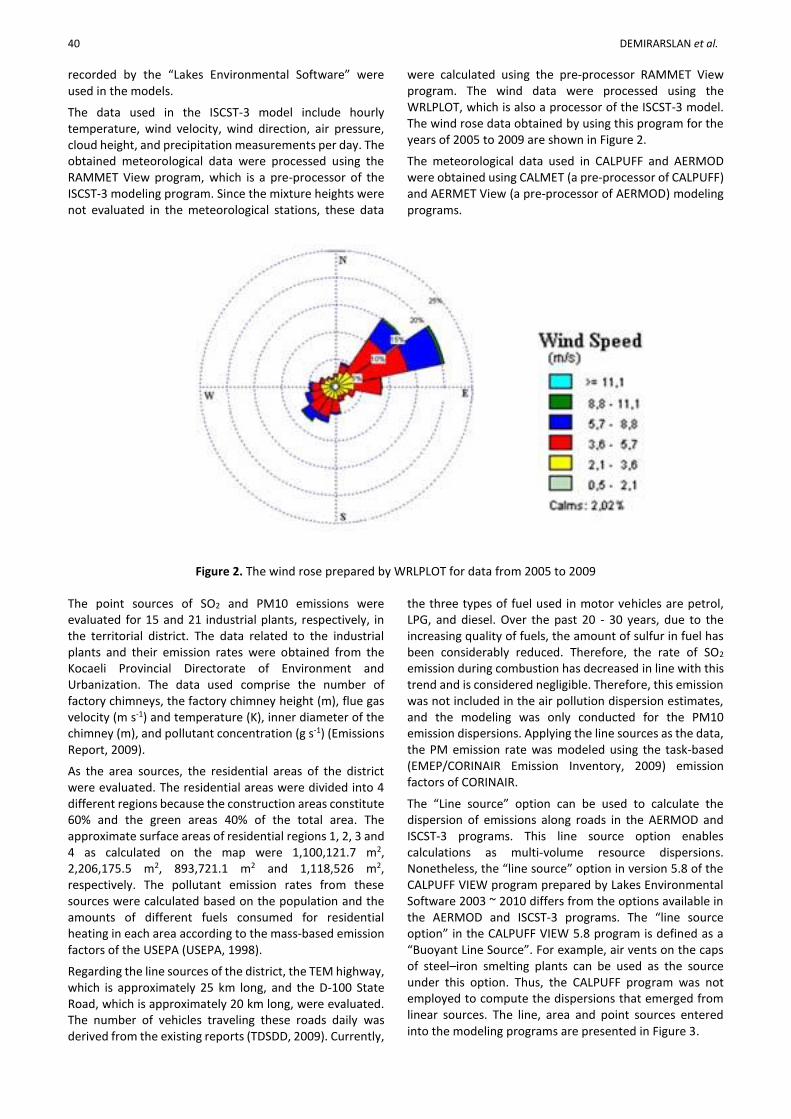
The “Line source” option can be used to calculate the dispersion of emissions along roads in the AERMOD and ISCST-3 programs. This line source option enables calculations as multi-volume resource dispersions. Nonetheless, the “line source” option in version 5.8 of the CALPUFF VIEW program prepared by Lakes Environmental Software 2003 ~ 2010 differs from the options available in the AERMOD and ISCST-3 programs. The “line source option” in the CALPUFF VIEW 5.8 program is defined as a “Buoyant Line Source”. For example, air vents on the caps of steel–iron smelting plants can be used as the source under this option. Thus, the CALPUFF program was not employed to compute the dispersions that emerged from linear sources. The line, area and point sources entered into the modeling programs are presented in Figure 3.


.

Figure 3. Point, area and line sources in the Körfez district

2.3. Ambient Air Quality Data

To evaluate the performance of the models, active measurements of SO2 and PM10 concentrations were obtained using mobile measurement vehicles located within the study area. SO2 and PM10 concentrations obtained from the station were daily averages, and their measurement results were annual. The SO2 measurements were performed using “the Environnement S.A. Model AF21M SO2 Analyzer”, whose measurement method depends on the UV lamp principle and whose measuring range is 0-1144 µg m-3. The PM10 measurements, on the other hand, was carried out via the “Andersen Instruments Model FH62I-N”, whose measurement method depends on the “beta-ray radiometric measurement principle“ and whose measuring range is 0-2400 µg m-3.

2.4. Statistical Methods for Evaluating the Models

To evaluate the predictions, the measured and predicted effects were compared by applying two different statistical methods. For the first method, the mean squared error (MSE) method presented in Equation (6) was used. In this equation, Co is the measured concentration, and Cp is the predictedexpected concentration value. The results of these calculations are dimensionless. This is the most common method for comparing the estimated and measured outcomes. A result less than 0.5 implies that the measured and modeled results are comparable (Ozkurt et al., 2013).

MSE=(Co̅-CP̅)

2

Co̅ CP̅̅̅̅

(6)

The second comparison method used was the fractional bias (FB) method given in Equation 7. The result range for FB must be between –2.00 (over-estimate) and +2.00 (very low estimate) (Botlaguduru, 2009). According to the literature, a suitable model corresponds to an FB value ranging from -0.7 to +0.7 (Demirarslan and Doğruparmak, 2016).

FB= 2 (Co̅-CP̅)

Co̅+CP̅

(7)

An ideal model corresponds to FB and MSE values equaling 0. However, models are not perfect. To identify whether a model is suitable, it is necessary to ascertain that it meets certain standards. For example, if the MSE is less than 0.5 and the FB is between -0.5 and 0.5, then the measured and estimated results overlap by 95% (Botlaguduru, 2009).

3. Results and Discussion

3.1. Modeling Results

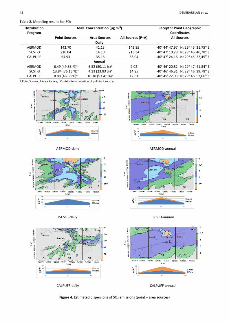
SO2 dispersions. Since the SO2 emissions from line sources were negligible, SO2 emissions from point and area sources were entered into the programs. The models were run using the daily (short term averaging period, 24 hours) and annual time (long term averaging period, 365 days) options separately for each type of source. These daily and annual results are given in Table 2. Table 2 presents the coordinates of the points giving the most intense SO2 emissions. The daily and annual dispersion maps are shown in Figure 4.

After the modeling results were analyzed, it was observed that the highest concentration values calculated by each program were different. The highest concentration was calculated by the ISCST-3 program when the modeling results from all of the sources were analyzed.

The contributions of contaminants to the total pollution (Table 2 and Figure 4) changed according to the modeling program and average time options.

For the SO2 emissions, the area sources were more prevalent according to the AERMOD and CALPUFF programs, and the point sources were more dominant than the area sources according to the ISCST-3 program. According to the dispersion maps (Figure 4), an intense concentration was observed in the field of N2 (the central part of the district) in both the daily and annual dispersion maps.


Table 2. Modeling results for SO2

Distribution Program

Max. Concentration (µg m-3) Receptor Point Geographic Coordinates

Point Sources Area Sources All Sources (P+A) All Sources

Daily

AERMOD 142.70 41.13 142.85 40o 44' 47,97'' N; 29o 45' 31,75'' E ISCST-3 210.04 14.10 213.34 40o 47' 10,28'' N; 29o 46' 40,78'' E

CALPUFF 64.93 35.16 66.04 40o 47' 24,16'' N; 29o 45' 22,45'' E

Annual

AERMOD 6.49 (49.88 %)a 6.52 (50.11 %)a 9.02 40o 46' 20,82'' N; 29o 47' 41,84'' E ISCST-3 13.84 (76.16 %)a 4.33 (23.83 %)a 14.85 40o 46' 46,31'' N; 29o 46' 39,78'' E

CALPUFF 8.88 (46.58 %)a 10.18 (53.41 %)a 12.51 40o 45' 22,03'' N; 29o 46' 52,06'' E

P:Point Source, A:Area Source, a Contribute to pollution of pollutant sources

AERMOD-daily AERMOD-annual

ISCST3-daily ISCST3-annual

CALPUFF-daily CALPUFF-annual

Figure 4. Estimated dispersions of SO2 emissions (point + area sources)

EVALUATION OF THREE POLLUTANT DISPERSION MODELS FOR THE ENVIRONMENTAL ASSESEMENT 43

PM10 dispersions. PM10 dispersion was modeled in two ways: PM10 emissions composed of point, area, and line sources were modeled using the AERMOD and ISCST-3 programs, and PM10 emissions composed of only point and area sources were modeled using the AERMOD, ISCST-

3 and CALPUFF programs. The results and the coordinates of the highest intensity point determined on the dispersion maps of PM10 emissions are given in Table 3. The daily and annual dispersion maps are shown in Figures 5 and 6.

Table 3. Modeling results for PM10

Distribution Program

Max. Concentration (µg m-3)

Receptor Point Geographic Coordinates

Point Sources Area Sources Line Sources All Sources

P+A+L All Sources

P+A All Sources

P+A+L All Sources

P+A

Daily

AERMOD 106.57 86.70 59.49 137.22 137.09 40o 47' 06.45'' N 29o 49' 18.46'' E

40o 47' 06.45'' N; 29o 49' 18.46'' E

ISCST-3 346.02 69.47 13.73 349.93 349.23 40o 47' 06.45'' N 29o 49' 18.46'' E

40o 47' 06.45'' N; 29o 49' 18.46'' E

CALPUFF 148.86 92.21 - - 149.88 - 40o 46' 53.30'' N; 29o 50' 05.27'' E

Annual

AERMOD 18.25

(44.16%)a

17.10 (41.38%)a

5.97 (14.44%)a 20.00 19.53

40o 46' 20.82'' N 29o 47' 41.84'' E

40o 46' 20.82'' N; 29o 47' 41.84'' E

ISCST-3 32.50

(68.87%)a

11.51 (24.39%)a 3.18 (6.73%)a 33.47 33.37

40o 47' 06.45'' N 29o 49' 18.46'' E

40o 47' 06.45'' N; 29o 49' 18.46'' E

CALPUFF 12.47

(31.83%)a 26.7 (68.16%)a - - 29.74 - 40o 46' 36.21'' N; 29o 45' 20.47'' E

P: Point Source, A: Area source, L: Line source aContribute to pollution of pollutant sources

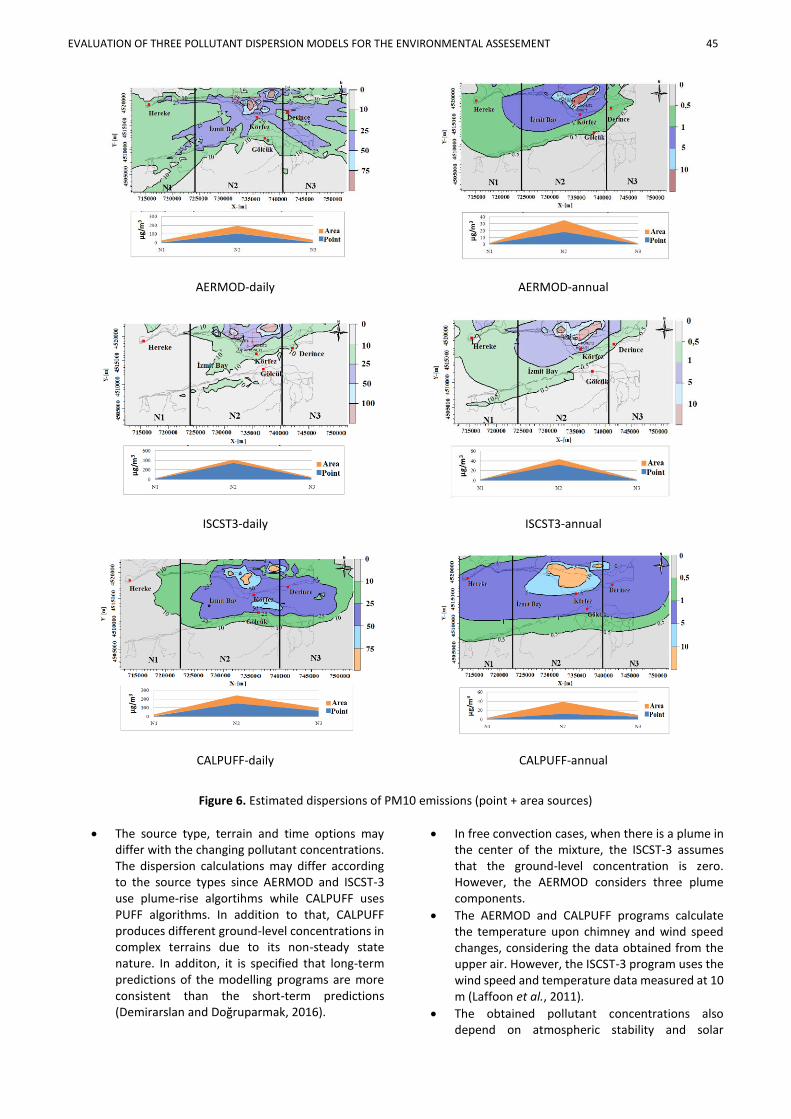
The highest concentration values according to different time options differed for each program (Table 3). The highest concentration was calculated by the ISCST-3 program, in addition to the results of SO2 emissions for all of the sources. The contribution of each pollutant source to the total contribution changed according to the modeling program and the average time used. Using the annual average time options, the point sources were the most polluting ones according to the AERMOD and ISCST-3 programs. However, the area sources were the most polluting source type according to the CALPUFF program for the PM10 emissions. Furthermore, the effect of line sources was less comparable to the other sources.

The daily and annual dispersion maps in Figures 5 and 6 show that an intense concentration was found in the N2 area (the central part of the district). The CALPUFF program could generate a larger dispersion map than the other programs.

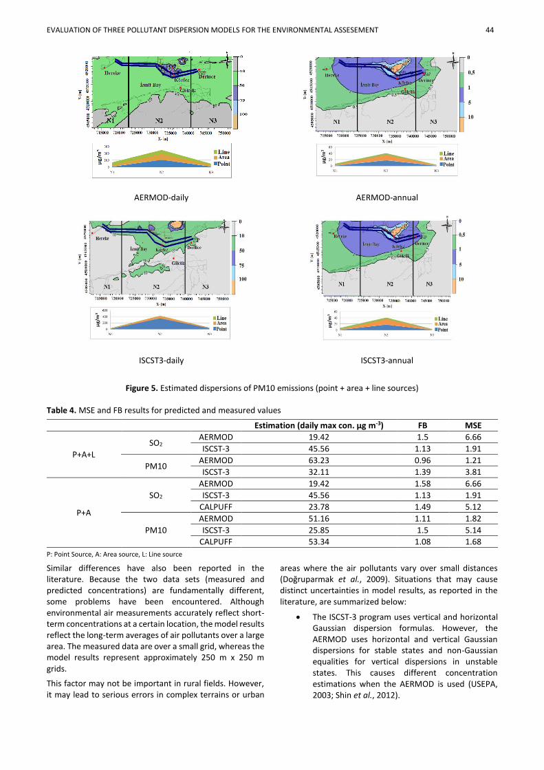
3.2. Evaluation of model performances

The statistical methods of MSE and FB were used to evaluate the performance of the models. The daily maximum concentrations of the measured and predicted results were used in the statistical calculations. In order to specify the predicted concentration for comparison, the

coordinates of the point where the active measurement was performed was determined and the concentration values at receptors (receptor is the 1074th point) corresponding to this coordinate were taken as a basis in the model programs. The obtained results are shown in Table 4.

Table 4 shows that the FB results obtained by modeling the point + area + line sources using the ISCST-3 and AERMOD programs are between +0.96 and +1.39. Values greater than zero indicate that the estimated values are lower than the measured results. Nevertheless, the results of the MSE analysis vary between 1.21 and 6.66, suggesting that the performance for estimating the contaminants is variable. The statistical evaluations of FB and MSE revealed that the results of the models differed for the various contaminants that were studied. In general, the AERMOD for PM10 emissions and the ISCST-3 for SO2 emissions are considered to have the best performance.

Considering the modeling results obtained from the three programs for point and area sources, the FB results vary between +1.08 and +1.58. However, the MSE results vary between 1.68 and 6.66. The performance evaluation of the models ranking from high to low was determined as CALPUFF > AERMOD > ISCST-3 for PM10 and ISCST-3 > CALPUFF > AERMOD for SO2.




Figure 5. Estimated dispersions of PM10 emissions (point + area + line sources)

Table 4. MSE and FB results for predicted and measured values

Estimation (daily max con. µg m-3) FB MSE

P+A+L

SO2 AERMOD 19.42 1.5 6.66

ISCST-3 45.56 1.13 1.91

PM10 AERMOD 63.23 0.96 1.21

ISCST-3 32.11 1.39 3.81

P+A

SO2

AERMOD 19.42 1.58 6.66

ISCST-3 45.56 1.13 1.91

CALPUFF 23.78 1.49 5.12

PM10

AERMOD 51.16 1.11 1.82

ISCST-3 25.85 1.5 5.14

CALPUFF 53.34 1.08 1.68

P: Point Source, A: Area source, L: Line source

Similar differences have also been reported in the literature. Because the two data sets (measured and predicted concentrations) are fundamentally different, some problems have been encountered. Although environmental air measurements accurately reflect short-term concentrations at a certain location, the model results reflect the long-term averages of air pollutants over a large area. The measured data are over a small grid, whereas the model results represent approximately 250 m x 250 m grids.

This factor may not be important in rural fields. However, it may lead to serious errors in complex terrains or urban

areas where the air pollutants vary over small distances (Doğruparmak et al., 2009). Situations that may cause distinct uncertainties in model results, as reported in the literature, are summarized below:

The ISCST-3 program uses vertical and horizontal Gaussian dispersion formulas. However, the AERMOD uses horizontal and vertical Gaussian dispersions for stable states and non-Gaussian equalities for vertical dispersions in unstable states. This causes different concentration estimations when the AERMOD is used (USEPA, 2003; Shin et al., 2012).




CALPUFF-daily CALPUFF-annual

Figure 6. Estimated dispersions of PM10 emissions (point + area sources)

The source type, terrain and time options may differ with the changing pollutant concentrations. The dispersion calculations may differ according to the source types since AERMOD and ISCST-3 use plume-rise algortihms while CALPUFF uses PUFF algorithms. In addition to that, CALPUFF produces different ground-level concentrations in complex terrains due to its non-steady state nature. In additon, it is specified that long-term predictions of the modelling programs are more consistent than the short-term predictions (Demirarslan and Doğruparmak, 2016).

In free convection cases, when there is a plume in the center of the mixture, the ISCST-3 assumes that the ground-level concentration is zero. However, the AERMOD considers three plume components.

The AERMOD and CALPUFF programs calculate the temperature upon chimney and wind speed changes, considering the data obtained from the upper air. However, the ISCST-3 program uses the wind speed and temperature data measured at 10 m (Laffoon et al., 2011).

The obtained pollutant concentrations also depend on atmospheric stability and solar


radiation (Botlaguduru, 2009). It is known that AERMOD and ISCST-3 could not perform dispersion calculations for the stability conditions where wind speed does not exceed 0.5 m s-1, unlike CALPUFF, which is a non-steady state program.

The CALPUFF was developed using observational wind data (wind speed and direction that are measured directly by instrumentation) and terrain on a precise scale, in contrast to the Gaussian plume model, allowing for calculations using this modeling program under calm weather conditions (Abdul-Wahab et al., 2011; Calpuff Dispersion Model, 2012). The elevation and the form of terrain were obtained from the WEBLAKES web site, yielding the coordinates of the modeled area. For the other two programs, these data, used as the receptor points, were entered manually. These two programs used the heights of the receptor points for terrain elevation, which may cause differences in the calculations (Demirarslan and Doğruparmak, 2016).

The observed differences are thought to be caused by the following:

- the lack of statistical data and the difficulty of recovering the available data in Turkey,

- the absence of emission factors for the conditions in Turkey,

- traffic conditions that do not sufficiently reflect their share of emissions (Doğruparmak et al., 2009),

- the undetermined relationship between the behavior of pollutants in the air and meteorological factors (USEPA, 2003),

- simplifications of data resources and limitations of facilities,

- the extrapolation of large areas of meteorological data for the selected regions,

- the simplification of the randomness of natural dispersions in the atmosphere (Calpuff Dispersion Model, 2012),

- the inability of the AERMOD and ISCST-3 programs to calculate receptor points within 1 m of the source when the receptor coincides with area sources (Villalvazo, 2007), and

- the lack of meteorological stations in Turkey, possibly causing region-specific meteorological data based on the satellite observations to be unrepresentative of the true sense of the study area.

3.3. Comparison of the Results with Limit Values

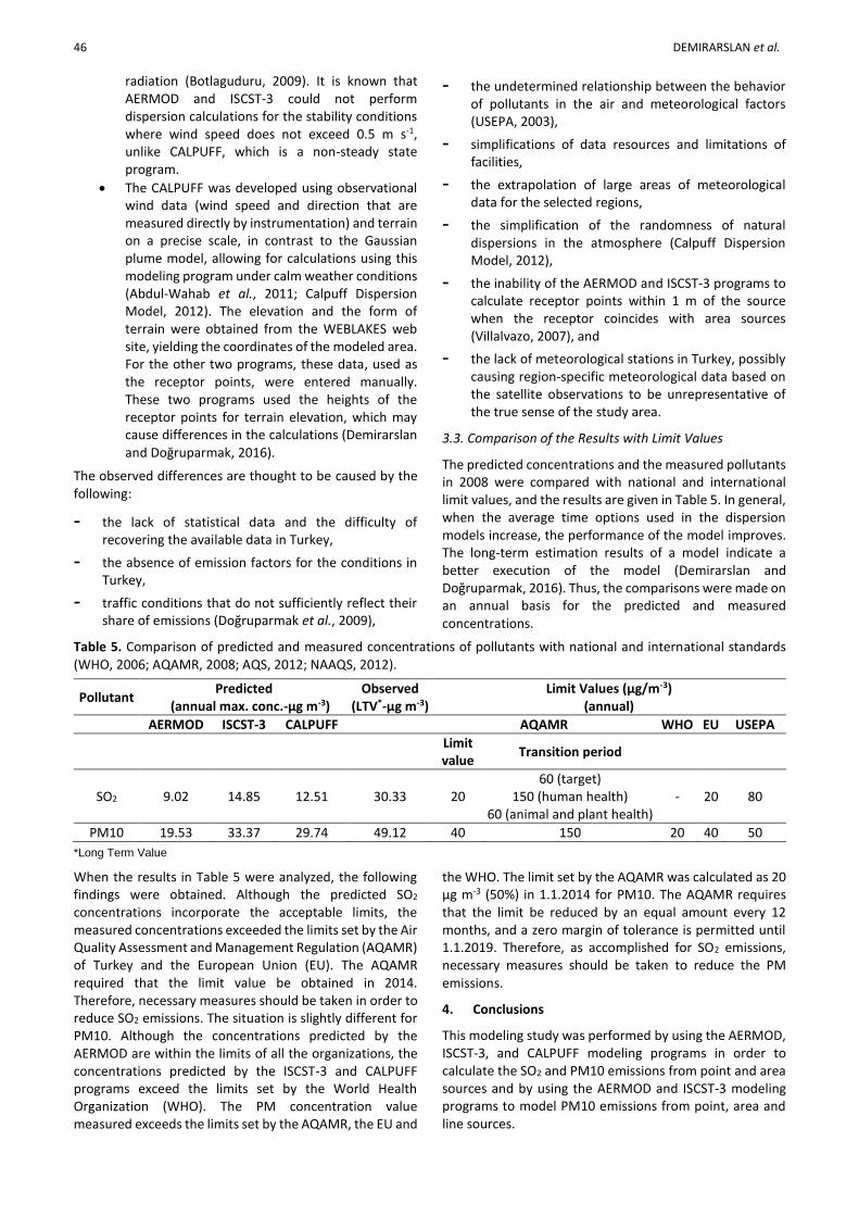
The predicted concentrations and the measured pollutants in 2008 were compared with national and international limit values, and the results are given in Table 5. In general, when the average time options used in the dispersion models increase, the performance of the model improves. The long-term estimation results of a model indicate a better execution of the model (Demirarslan and Doğruparmak, 2016). Thus, the comparisons were made on an annual basis for the predicted and measured concentrations.

Table 5. Comparison of predicted and measured concentrations of pollutants with national and international standards (WHO, 2006; AQAMR, 2008; AQS, 2012; NAAQS, 2012).

Pollutant Predicted

(annual max. conc.-μg m-3) Observed

(LTV*-μg m-3) Limit Values (µg/m-3)

(annual)

AERMOD ISCST-3 CALPUFF AQAMR WHO EU USEPA

Limit value

Transition period

SO2 9.02 14.85 12.51 30.33 20 60 (target)

150 (human health) 60 (animal and plant health)

- 20 80

PM10 19.53 33.37 29.74 49.12 40 150 20 40 50

*Long Term Value

When the results in Table 5 were analyzed, the following findings were obtained. Although the predicted SO2 concentrations incorporate the acceptable limits, the measured concentrations exceeded the limits set by the Air Quality Assessment and Management Regulation (AQAMR) of Turkey and the European Union (EU). The AQAMR required that the limit value be obtained in 2014. Therefore, necessary measures should be taken in order to reduce SO2 emissions. The situation is slightly different for PM10. Although the concentrations predicted by the AERMOD are within the limits of all the organizations, the concentrations predicted by the ISCST-3 and CALPUFF programs exceed the limits set by the World Health Organization (WHO). The PM concentration value measured exceeds the limits set by the AQAMR, the EU and

the WHO. The limit set by the AQAMR was calculated as 20 µg m-3 (50%) in 1.1.2014 for PM10. The AQAMR requires that the limit be reduced by an equal amount every 12 months, and a zero margin of tolerance is permitted until 1.1.2019. Therefore, as accomplished for SO2 emissions, necessary measures should be taken to reduce the PM emissions.

4. Conclusions

This modeling study was performed by using the AERMOD, ISCST-3, and CALPUFF modeling programs in order to calculate the SO2 and PM10 emissions from point and area sources and by using the AERMOD and ISCST-3 modeling programs to model PM10 emissions from point, area and line sources.


As a result of the study; it was seen that the highest concentration was calculated by the ISCST-3 program. When the results obtained by modeling all of the point and area sources by the three programs were investigated, the maximum annual concentrations according to the AERMOD, CALPUFF and ISCST-3 programs were calculated as 9.02, 14.85, and 12.51 µg m-3 for SO2 and 19.53, 33.37, and 29.74 µg m-3 for PM10, respectively. The maximum concentrations of PM10 obtained by modeling all of the point, area and line sources using the AERMOD and ISCST-3 programs were 20.00 and 33.47 µg m-3, respectively. These results clearly indicate that line sources exert less of an effect than the other sources.

Furthermore, when the contributions of the pollutant sources on pollution were evaluated, certain differences were observed. According to individual modeling results were obtained using point and area sources by three programs, the prevalent sources for SO2 pollution are the area sources for the AERMOD and CALPUFF programs, while point sources for the ISCST-3 program. On the other hand, according to the AERMOD and ISCST-3 programs, the point sources were dominant, and according to the CALPUFF, the area sources were dominant for PM10.

The dispersion map of the study area was divided into three regions, and intense concentrations were observed in the central area, particularly in the Körfez district, which may be due to greater amounts of emissions released into the atmosphere.

The fractional bias results (between +1.08 and +1.58) and the mean square error results (between 1.68 and 6.66) for evaluating the performance of the models varied according to both the type of pollutant and the time options. The predicted results were lower than the measured results. In these studies, the accuracy of the model results depends on correct measurements of the meteorological parameters over the study area and elaborate and accurate emission inventories of all the sources (Bhanarkar et al., 2005). The model estimates can be further changed using substantial data for the input parameters (Yegnan et al., 2002). However, difficulties in obtaining actual data are a limitation for this type of study. According to the fractional bias/mean square error results, an overall ranking regarding the modeling performance is as follows: CALPUFF > AERMOD > ISCST-3 for PM10 and ISCST-3 > CALPUFF > AERMOD for SO2.

Finally, when the predicted and measured values were compared with the national and international limit values, it was determined that there were certain measures that would reduce both the SO2 and PM10 emissions. Considering the adverse effects of SO2 and PM10 emissions, monitoring these emissions in the urban air and interpreting the results are very important for preventing such effects. This is an important step for “Clean Air Action Plans”.

Acknowledgments

This research was financially supported by the Scientific Research

Projects Unit of Kocaeli University (Project no. 2009/55)

References

Abdul-Wahab S., Sappurd A. and Al-Damkhi A. (2011), Application

of California puff (CALPUFF) Model: a case study for Oman,

Clean Technologies and Environmental Policy, 13, 177–189.

Abdul-Wahab S., Chan K., Elkamel A. and Ahmadi L. (2014), Effects

of meteorological conditions on the concentration and

dispersion of an accidental release of H2S in Canada,

Atmospheric Environment, 82, 316-326.

AQAMR (Air Quality Assessment and Management Regulation)

(2008), T.C. The Ministry Of Environment and Urban Planning,

R.G.S. 26898 R.G.T. 06.06.2008.

AQMG (Air Quality Model Guideline) (2010),

http://environment.alberta.ca, Accessed 11 December 2010.

AQS (Air Quality Standards) (2012),

http://ec.europa.eu/environment/air/quality/standards.htm

Accessed 11 December 2014.

Bhanarkar A.D., Goyal S.K., Sivacoumar R. and Chalapati Rao C.V.

(2005), Assessment of contribution of SO2 and NO2 from

different sources in Jamshedpur region, India, Atmospheric

Environment, 39(40), 7745-7760.

Botlaguduru V.S.V. (2009), Comparison of AERMOD and ISCST3

models for particulate emissions from ground level sources,

Master of Science, Texas A&M University, Texas USA.

British Columbia Ministry of Environment (2008), Environmental

Protection Division Environmental Quality Branch, Air

Protection Section, Guidelines for Air Quality Dispersion

Modelling in British Columbia.

Calpuff Dispersion Model (2012), Appendix D. Roberts Bank

Container Expansion Project Deltaport Third Berth,

http://www.portmetrovancouver.com, Accessed 21 July

2012.

Civan M.Y. and Kara M. (2016), Risk assessment of PBDEs and

PAHs in house dust in Kocaeli, Turkey: levels and sources,

Environmental Science and Pollution Research, 23, 369-384.

Clappier A., Pisoni E. and Thunis P. (2015), A new approach to

design source a receptor relationships for air quality

modeling, Environmental Model and Software, 74, 66-74.

Cui H., Rentai Y., Xiangjun X., Cuntian X. and Jinming Y. (2011), A

tracer experiment study to evaluate the CALPUFF real time

application in a near-field complex terrain setting.

Atmospheric Environment, 45(39), 7525-7532.

Demirarslan K.O. and Doğruparmak Ş.Ç. (2016), Determination of

performance and application of the steady-state models and

the lagrangian puff model for environmental assessment of

CO and NOX emissions, Polish Journal Environmental Studies,

25(1), 83-96.

Diaz J.C.G. and Zafrilla J.M.G. (2012), Uncertainty and sensitive

analysis of environmental model for risk assessments: an

industrial case study, Reliability Engineering & System Safety,

107, 16-22.

Doğruparmak Ş.Ç., Karademir A. and Ayberk S. (2009), Dispersion

model predictions of NOX emissions: case study from Kocaeli,

Turkey, Fresenius Environmental Bulletin, 18(8), 1497-1502.

Doğruparmak Ş.Ç., Keskin A.G., Yaman S. and Alkan A. (2014),

Using principal component analysis and fuzzy c–means

clustering for the assessment of air quality monitoring,

Atmospheric Pollution Research, 5, 656-663.

EMEP/CORINAIR Emission Inventory (2009),

http://www.eea.europa.eu/publications, Accessed: 12

October 2010.

ISCST-3 Tech Guide (2009), http://www.weblakes.com, Accessed

23 February 2009.

http://ec.europa.eu/environment/air/quality/standards.htm

http://www.eea.europa.eu/publications,%20Accessed:%2012%20October%202010

http://www.eea.europa.eu/publications,%20Accessed:%2012%20October%202010


Jeong S.J. (2011), CALPUFF and AERMOD dispersion models for

estimating odor emissions from industrial complex area

sources, Asian Journal of Atmospheric Environment, 5(1), 1-7.

Korfez District, http://www. körfez.bel.tr/tr/default.aspx,

Accessed: 23 April 2009.

Laffoon C., Rinaudo J., Soule R., Bowie T., Meyers C., Madura R. L.

and Pakunpanya S.P. (2011), Developing state-wide modeling

guidance for the use of AERMOD–a workgroup’s experience,

http://files.abstractsonline.com, Accessed 07 April 2011.

Markiewicz M. (2008), Modelling of the air pollution dispersion,

http://manhaz.cyf.gov.pl, Accessed 25 April 2010.

Macintosh D.L., Stewart J.H., Myatt T.A., Sabato T.E., Flowers G.C.,

Brown K.W., Hlinka, D.J. and Sullivan D.A. (2010), Use of

CALPUFF for exposure assessment in a near-field, complex

terrain setting, Atmospheric Environment, 44(2), 262-270.

Mokhter M.M., Hassim M.H. and Taib R.M. (2014), Health risk

assessment of emissions from a coal-fired power plant using

AERMOD modeling, Process Safety and Environmental

Protection, 92(5), 476-485.

NAAQS (National Ambient Air Quality Standards) (2012), U.S.

Environmental Protection Agency.

Ozkurt N., Sari D., Akalin N. and Hilmioğlu B. (2013), Evaluation of

the impact of SO2 and NO2 emissions on the ambient air-

quality in the Çan–Bayramiç region of northwest Turkey

during 2007–2008, Science of the Total Environment, 456-457,

254-266.

Rojas A.L.P. and Venegas L.E. (2010), Interannual variability of

estimated monthly nitrogen deposition to coastal waters due

to variations of atmospheric variables model input,

Atmospheric Research, 96(1), 80-102.

Rood A.S. (2014), Performance evaluation of AERMOD, CALPUFF

and legacy air dispersion models using the winter validation

tracer study dataset, Atmospheric Environment, 89, 707-720.

Shin H.M., Ryan P.B., Vieira V.M. and Bartell S.M. (2012),

Modeling the air-soil transport pathway of perfluorooctanoic

acid in the Mid-Ohio Valley using linked air dispersion and

vadose zone models, Atmospheric Environment, 51, 67-74.

Silva E.J.G., Tirabassi T., Vilhena M.T. and Buske D. (2013), A puff

model using a three-dimensional analytical solution for the

pollutant diffusion process, Atmospheric Research, 134,

131-136.

TDSDD (The Department of Strategic Development Division of

Transport Cost and Productivity) (2009), The annual average

daily traffic values of highways and state roads transportation

information according to traffic zone in 2008.

USEPA (United States Environmental Protection Agency) (1998),

Technology transfer network clearinghouse for inventories &

emission factors, fifth edition.

USEPA (United States Environmental Protection Agency) (2003),

AERMOD: latest featuresand evaluation results EPA-454/R-

03-003, Research Triangle Park, North Carolina, Office of Air

Quality Planning and Standards Emission, Monitoring and

Analysis Division.

Villalvazo L., Davila E. and Reed G. (2007), Guidance for air

dispersion modeling, San Joaquin Valley Air Pollution Control

District, 01/07 Rev 2.0, 36.

Wang L., Parker D.B., Parnell C.B., Lacey R.E. and Shaw B.W.

(2006), Comparison of CALPUFF and ISCST3 models for

predicting downwind odor and source emission rates,

Atmospheric Environment, 40, 4663-4669.

WHO (World Health Organization) (2006), Air quality guidelines

for particulate matter, ozone, nitrogen dioxide and sulfur

dioxide.

Yegnan A., Williamson D.G. and Graettinger A.J. (2002),

Uncertainty analysis in air dispersion modeling,

Environmental Modelling & Software, 17(7), 639-649.

Documents

Evaluation of three pollutant dispersion models for the ... · The AERMOD model is a linear steady-state plume model. The formulations of the AERMOD program are grounded along the