1

Global Plume-fed Asthenosphere Flow: (1) Motivation and Model Development

Michiko Yamamoto, Jason Phipps Morgan

Institute for the Study of the Continents, EAS Department, Cornell University

(my83@cornell.edu, jp369@cornell.edu)

W. Jason Morgan

EPS Department, Harvard University

ABSTRACT

This study explores a conceptual model for mantle convection in which buoyant

and low viscosity asthenosphere is present beneath the relatively thin lithosphere of ocean

basins and regions of active continental deformation, but is less well developed beneath

thicker-keeled continental cratons. We start by summarizing the concept of a buoyant

plume-fed asthenosphere, the alternative implications this framework has for the roles of

compositional and thermal lithosphere, and the sinks of asthenosphere by forming

compositional lithosphere at ridges, by plate cooling where-ever the thermal boundary

layer extends beneath the compositional lithosphere, and by dragdown of buoyant

asthenosphere along the sides of subducting slabs. We also review the implied origin of

hotspot swell roots by melt-extraction from the hottest portions of upwelling plumes

analogous to the generation of compositional lithosphere by melt-extraction beneath a

spreading center. The plume-fed asthenosphere hypothesis requires an alternative to

‘distinct source reservoirs’ to explain the differing trace element and isotopic

2

characteristics of Ocean Island Basalt (OIB) and Mid-Ocean Ridge Basalt (MORB)

sources; it does so by having the MORB source be the plum-depleted and buoyant

asthenospheric leftovers from progressive melt-extraction within upwelling plumes,

while the preferential melting and melt-extraction of more-enriched plum components is

what makes OIB of a given hotspot typically fall within a tube-like geometric isotope

topology characteristic to that hotspot. Using this conceptional framework, we construct a

thin-spherical-shell finite element model with a ~100-km-scale mesh to explore the

possible structure of global asthenosphere flow. Lubrication theory approximations are

used to solve for the flow profile in the vertical direction. We assess the correlations

between predicted flow and geophysical observations, and conclude by noting current

limitations in the model and the reason why we currently neglect the influence of

subcontinental plume upwelling for global asthenosphere flow.

INTRODUCTION

For the past dozen years we have been actively exploring the consequences of a

conceptual model of mantle convection in which discrete upwelling plumes feed a weak

asthenospheric boundary layer underlying the relatively thin oceanic lithosphere (Fig. 1).

In this scenario of mantle convection (Phipps Morgan and Smith 1992; Phipps Morgan,

Morgan et al. 1995; Phipps Morgan, Morgan et al. 1995; Phipps Morgan 1997; Phipps

Morgan 1998; Phipps Morgan 1999; Phipps Morgan and Morgan 1999), a plume-fed

asthenosphere is viewed as an almost inevitable consequence of the fact that the hottest

and most buoyant mantle will rise as ‘plumes’ (Morgan, 1971) until its ascent is impeded

3

at the base of the lithosphere. At this point plume material will pond and flow laterally

beneath the base of the lithosphere until it: (1) increases in viscosity either by cooling or

by drying out through decompression melting to be transformed into part of the overlying

lithosphere; (2) is entrained and dragged down by a subducting slab.

This conceptual model is not new, the key idea was first presented in 1972 by

Deffeyes (Deffeyes 1972) as an implication of Morgan’s mantle plume hypothesis

(Morgan, 1971). The conceptual model shares many aspects of conventional mantle flow

models. In it, the cooling, growth, and subduction of oceanic lithosphere is the heat

engine that ultimately drives mantle convection (Turcotte and Oxburgh 1967; Elsasser

1971). We also accept and build from the conventional interpretation of seismological

evidence that slabs often subduct deep into the mantle, e.g. this scenario is a variant of

‘whole mantle flow’. However, this scenario differs from the conventional model in its

important roles for plume upwelling, the rheological and density effects of melt

extraction, and the importance of the mantle having a fine-scale marble-cake or plum-

pudding lithologic variation as a byproduct of the geochemical heterogeneity introduced

by the persistent subduction of compositionally distinct sediments, ocean crust, and

lithosphere, and subsequent stirring and stretching of these lithologic heterogeneities

during mantle flow.

This scenario for asthenosphere flow also has some aspects in common with

previous suggestions for a shallow upper mantle ‘counterflow’ from regions of trench

supply of slab inputs to the upper mantle to ridge consumption of upper mantle. Schubert

and Turcotte (1972) presents the basic hypothesis, while Harper (1978), Chase (1979),

and Parmentier and Oliver (1979) developed models based upon this hypothesis to

4

predict the global pattern of asthenosphere counterflow. There is a major similarity

between our preferred model and these previous ones — typically there is counterflow of

asthenosphere away from a subduction zone, although in our scenario is much less.

(Tonga is one place where our models differ in a testable way from these counterflow

models; in our models the predicted asthenosphere flow is nearly trench parallel – as

opposed to the trench-perpendicular prediction of counterflow models – as it heads

southward towards the southern ridge system.) In our scenario, the counterflow is entirely

within the asthenosphere. The material that ‘counterflows’ is the fraction of

asthenosphere that, because of its buoyancy, resists dragdown by the slab descending into

the deeper mantle (i.e. the subducted slab doesn’t counterflow). Contrariwise, in pure

counterflow models, the source of new upper mantle material is the injection of the entire

slab into this upper mantle — an assumption that now seems disproven by tomographic

images of subducting slabs that are conventionally interpreted to subduct through the

upper mantle, and often deep into the lower mantle.

There are several big differences between plume-fed asthenosphere flow and

counterflow models; in the plume-fed flow scenario, slabs remove subducted lithosphere

from the shallow mantle (instead of reinjecting ‘asthenosphere’ into the upper mantle as

in pure counterflow models), and in the plume-fed flow scenario it is upwelling mantle

plumes that provide the supply of ‘new’ asthenosphere to the shallow mantle. For further

discussion of the similarities and differences between these scenarios see Phipps Morgan

and Smith (1992) and Phipps Morgan et al. (1995a).

We realize that readers are likely to be unfamiliar with how this conceptual model

presents a coherent alternative. Thus we will begin this paper with an overview of this

5

scenario and how it involves the reinterpretation of several basic observations on hotspots

and mid-ocean ridge volcanism. In general, we will highlight observations that postdate

a previous paper (Phipps Morgan et al. 1995a) discussing observational evidence that

favors the existence of a plume-fed asthenosphere beneath the ocean basins.

The basic element of the conceptual model is that the mantle’s upward mass-

balance to the downward subduction of cold slabs is by upwelling in mantle plumes

followed by lateral flow in a hot, weak, and buoyant asthenosphere layer. The picture of

focused convective upwelling in mantle plumes is essentially the same as in Morgan’s

original plume hypothesis (Morgan, 1971;1972). Flow in the asthenosphere is necessary

to redistribute the plume-fed asthenosphere from the localized regions of plume

upwelling to the regions where asthenosphere is consumed by lithosphere formation at

mid-ocean ridges (a large concentrated sink), subsequent off-axis lithosphere growth by

surface cooling (a large diffuse sink), and asthenospheric downdragging or entrainment

along the sides of dense subducting slabs (a smaller concentrated sink).

The three main issues of contention for this conceptual model are: (1) Is there a

shallow asthenosphere layer that is hotter than underlying mantle in terms of its potential

temperature, hence weaker and more buoyant?; (2) Is the upwelling plume flux large

enough to counterbalance asthenosphere consumption by plate subduction?; (3) If plumes

feed ridges, then how are the distinct geochemical differences between hotspot (plume)

basalts and mid-ocean ridge basalts created and maintained? Each of these issues has

been discussed and resolved to our provisional satisfaction in previous publications.

However, because these successful resolutions have been published separately, the

potential of the conceptual model to provide a cohesive internal framework for

6

understanding the flow and chemical evolution of the mantle is likely to have been

underappreciated.

Asthenosphere

The existence of a shallow asthenosphere region beneath oceanic plates is central

to our model. Much of the evidence for such a hot, weak, and buoyant asthenosphere is

so familiar that it is perhaps too easily taken for granted. The oldest and strongest

observation is that the seismic low-velocity zone (LVZ) has been used to imply that

lower viscosity mantle is to be found beneath oceanic lithosphere and the thinner regions

of continental lithosphere. (The observation has two parts. The first is the existence of a

seismic low-velocity zone between ~80-300 km depths (Gutenberg, 1959; Dziewonski

and Anderson, 1981) in average 1-D global models that, being a global average, are

biased towards the average velocity structure beneath the 60% of the world lying beneath

oceanic lithosphere. The second part is that the lithosphere beneath Proterozoic and

Archean regions of the continents is seismically fast in the depth-interval of the global

LVZ. Anderson (1989) has a good summary of these well-established seismic

observations.)

Recent observations that highlight these well-known seismic characteristics are

shown in Figures 2 and 3. Figure 2 (Gaherty et al., 1999) shows the average 1-D seismic

velocity structure along transects that cross largely ocean seafloor (Central Pacific in 2a,

Phillipine Sea in 2b) and an Archean Shield province in Australia (Fig. 2c). A region

with lower seismic shear-wavespeeds begins roughly ~90-110 km beneath oceanic

lithosphere, at depths explicable as the thickness an oceanic plate would cool in ~60-100

7

Ma at Earth’s surface. Beneath the Archean part of Australia the seismically fast region

persists to depths of ~250-300 km where a much smaller LVZ is found. Figure 3

(Ekstrom and Dziewonski 1998; Nettles 2005) shows a complementary map of global

seismic shear wavespeed variations as imaged by surface waves in the ~50-200 km

depth-interval. Here the roots of Archean and Proterozoic continental regions are

typically 5% faster (=blue) in comparison to the slower (red) regions beneath oceanic

seafloor and areas of active continental deformation. Even though the lateral averaging

of this map in sub-oceanic regions is >1000km so that only the large-scale oceanic plate

cooling with age is evident within the ocean basins, this figure clearly shows this first-

order difference between subcontinental and suboceanic regions. Note that even the

Australian and Indian continental shields on the rapidly moving Indo-Australian Plate

have fast seismic wavespeeds, which means this is an effect associated with roots/keels

that move with continents, not with possible longlived and deeper mantle structures

associated with the ‘memory effect’ of a Pangea supercontinent. The cartoon structure

that we infer (Fig. 1) for the differences between continental and oceanic lithosphere is

similar to that shown by Gung et al. (2003).

Plume-fed Asthenosphere

We think the likeliest way to form the asthenosphere is for it to be plume-fed, i.e.

fed by naturally occurring buoyant upwellings of hotter than average mantle. In this

conceptual model, we imagine the asthenosphere layer to be hotter than underlying

mantle because it is formed from the most recent upwellings of hotter than average

mantle; buoyant upwellings that have displaced downwards any preexisting cooler and

8

denser asthenosphere as they spread out beneath the base of the lithosphere. Most likely

the asthenosphere is hotter in an absolute sense than its lithospheric lid or mantle base so

that it conductively loses heat through both its top and base. If not hotter in an absolute

sense than underlying mantle, then it remains hotter in terms of its potential temperature

(its temperature relative to the upper mantle adiabatic temperature gradient of ~0.3-

0.4K/km), since downward heat conduction can only cool the asthenosphere to the same

temperature as its underlying mantle and no cooler. Thus the base of the asthenosphere

will be intrinsically buoyant with respect to underlying mantle since its potential density

is lower. Concepts of potential temperature and potential density (density corrected for

variations along an adiabat) are well appreciated in oceanography since oceans typically

exhibit horizontal ‘isopycnal’ flow that occurs in layers stratified by increasing potential

density with increasing depth. However these concepts are uncommon in mantle

convection.

Melt-extraction-induced strengthening of mantle: effects on the generation of a

compositional lithosphere and on forming resite roots to hotspot swells.

Here our thinking has been highly influenced by Shun Karato’s suggestion in

1986 (Karato 1986) that the formation and extraction of a partial melt, because it

dehydrates the residue due to preferential concentration of water into the melt, increases

the viscosity of the residue by more that an order of magnitude. Karato’s logic was since

intracrystalline water has a strong weakening effect on the rheology of mantle olivine,

melt extraction from a peridotite may induce, by preferential extraction of ‘incompatible’

intracrystalline water into the melt phase, an increase in the viscosity of the dehydrated

9

restite left over after melt extraction. Phipps Morgan (1987, p. 1240) suggested that this

effect might lead to the formation of a more viscous (~1021 Pa-s) mantle region from ~10-

70 km depths beneath mid-ocean ridges in which plate-spreading-induced viscous

pressure gradients would be strong enough to focus melt to the spreading axis. Later,

Phipps Morgan (Phipps Morgan 1994; Phipps Morgan 1997) used the term

‘compositional lithosphere’ to distinguish between thermal lithosphere that grows by heat

loss through the seafloor and the stronger-than-asthenosphere ~70km thick restite layer

created by decompression melting and melt extraction at a spreading center (cf. Figure 1).

At that time we also realized that hotspot melting might also lead to the creation

of a similar root underlying a hotspot swell as the peridotites in the hottest central regions

of an upwelling plume melt beneath ‘normal’ oceanic lithosphere (Phipps Morgan et al.

1995b). The rate of subsequent lateral spreading of the Hawaiian swell was used to infer

the viscosity of the restitic swell root to be of order ~3x1020-1021 Pa-s (Phipps Morgan et

al. 1995b). Soon after, Greg Hirth and Dave Kohlstedt wrote an influential paper that

documents and reaffirms the basic plausibility of melt-extraction-linked strengthening of

restitic mantle and then discusses several applications of this idea for the growth and

evolution of oceanic lithosphere (Hirth and Kohlstedt 1996).

The two most important implications of these ideas for asthenosphere flow are:

(1) Mid-ocean ridges are the sites where enough asthenosphere is consumed by

decompression-melting-induced desiccation during plate extension to create a ~60-km-

thick compositional lithosphere underlying the ocean crust. In comparison to lithospheric

growth by conductive heatloss through the seafloor, this effect leads to much more

focused asthenosphere consumption at mid-ocean ridges, and the existence of a large

10

region between mid-ocean ridges and ~50 Ma seafloor where asthenosphere does not

further accrete to the lithosphere, as asthenosphere does not accrete to the cooling plate

until the thermal boundary layer extends beneath the >~60 km thickness of the

compositional lithosphere (Phipps Morgan 1994; Hirth and Kohlstedt, 1996; Phipps

Morgan 1997; Yale and Phipps Morgan 1998; Lee et al., 2005).

(2) The plume-flux ‘estimated’ by the sizes of hotspot swells (Davies 1988; Sleep

1990) is a misestimate. In their scenario (Fig. 4a), the regional uplift of a hotspot swell

reflects the entire upwelling flux of buoyancy plume material – all of the upwelling

plume material is refracted (i.e. bent) and dragged beneath the moving oceanic

lithosphere. (This scenario also supposes that the ambient sub-lithospheric

‘asthenosphere’ is stronger than upwelling plume material so that it is the resistance of

the surrounding ~1020 Pa-s mantle to intrusion by the spreading plume material (Olson

1990) that ultimately limits the lateral spreading of the low-viscosity swell root.)

However, in our preferred conceptual model (Fig. 4b), the swell root is not the

total plume flux. Rather, it reflects only a small fraction of the upwelling plume flux —

the hottest central flux of the upwelling plume. If the hotspot swell root consists of

higher-viscosity restite resulting from sufficient melt-extraction to dry the most heavily

melted peridotite within the upwelling and melting plume, then the size of a hotspot swell

reflects just the fraction of upwelling plume material that melts enough to create a strong

swell root. (In this conceptual model (Fig. 4b), the swell root is more viscous than

surrounding less-melted or unmelted asthenosphere, so that it is the viscosity of the swell

root itself (~3x1020 Pa-s beneath Hawaii) that ultimately limits its spreading – see further

discussion in (Phipps Morgan et al. 1995b)).

11

Note that in this hypothesis for making a swell root, the buoyancy of the swell

root is only due in part to its depleted composition since the swell root is also hotter than

surrounding asthenosphere. Because the swell root is more dehydrated and more viscous

than surrounding asthenosphere, both the thermal and the compositional buoyancy of the

swell root support the relief of the overlying hotspot swell. (Below we will assess in more

detail the question of how buoyancy changes in response to melt extraction.) This aspect

of the restite swell root model has been recently misstated in critiques of the restite swell

root model on page 316 of (Davies, 1999) and page 513 of (Schubert et al. 2001). Both

critiques incorrectly presuppose that all of the buoyancy supporting the hotspot swell in

the resite-swell root model must be due to its depleted composition. In fact, in Phipps

Morgan et al.’s (1995b) more detailed assessment of the amounts of buoyancy generated

by hotspot melting, the conclusion was that the thermal and chemical buoyancy in the

swell root and the chemical buoyancy of the thickened crust should all contribute roughly

equal amounts to the relief of the swell.

For example, the differences between Schubert et al.’s (2001) estimate of

depletion swell-support and ours stems from their use of a much smaller estimate for

Hawaiian volcanic production, and, to a lesser degree, to their assumption of a 33%

larger typical Hawaiian swell. Page 8060 of Phipps Morgan et al. (1995b) presents the

reasoning underlying an estimate of the basalt production rate at Hawaii to be 0.25

km3/yr (Note that this estimate is very similar to Robinson and Eakin’s (2006) more

recent estimate of 0.21 km3/yr), while (Schubert et al., 2001) use the production rate of

0.1 km3/yr that is apparently based on a 1970’s estimate ((BVSP) 1981) of Hawaiian

crustal thickening that was inferred prior to the collection of a good seismic cross-section

12

across the Hawaiian chain. Similarly Schubert et al. (2001) use an estimate by (Sleep

1990) of 8700 kg/s for the ‘buoyancy flux’ associated with the Hawaiian swell that

corresponds to the maximum values estimated by us (crosssections B&C in Table 1 of

Phipps Morgan et al. (1995b)), while the average of profiles A-K in Table 1 of Phipps

Morgan et al. (1995b) implies a swell buoyancy flux of only 6070 kg/s. With our estimate

of 0.25 km3/yr of basalt production linked to the creation of the Hawaiian swell, the

reasoning in Phipps Morgan et al. (1995b) would imply that the swell root’s depletion

buoyancy supports 2285 kg/s and the swell root’s thermal buoyancy supports 2665 kg/s

of the swell buoyancy flux, and off-island basaltic intrusions support the remaining 900

kg/s of the time-averaged Hawaiian swell buoyancy flux. Davies’ (1999) conclusions

ultimately depend upon his use of an estimate for basalt production at Hawaii of 0.03

km3/yr, a factor of 3 lower than that used by (Schubert et al. 2001) and almost a factor of

8 lower than our preferred estimate of 0.25 km3/yr for the recent rate of Hawaiian

volcanism or Robinson and Eakins’ (2006) similar recent estimate of 0.21 km3/yr.

(Somewhat curiously, Davies (1999) refers to (Phipps Morgan et al. 1995) for his 0.03

km3/yr estimate, apparently basing his estimate upon the seamount-chain cross-section

area shown in Table 1 and Figure 2b of (Phipps Morgan et al. 1995) multiplied by the

~0.1m/yr motion of the Pacific Plate over the Hawaiian hotspot. However, Figure 2a of

(Phipps Morgan et al. 1995) shows seismic measurements by (ten Brink and Brocher

1987) that imply that profile D with a topographic cross-sectional area of 343km2, is

actually associated with crustal thickening of ~12km over a width of ~200km, i.e.

associated with a magmatic cross-sectional area of 2400km2 and an implied volcanic

production rate of 0.24 km3/yr instead of 0.03 km3/yr.). If Davies had used Robinson and

13

Eakins’ (2006) or our preferred rates for Hawaiian volcanism and for the buoyancy flux

associated with the Hawaiian swell, then his approach would also have led to our

preferred conclusions.

Finally, a highly viscous swell root should be able to more efficiently excavate the

base of the overlying oceanic lithosphere, which will augment swell buoyancy as it

replaces cooler lithosphere instead of warm asthenosphere by the hot swell root. If 20 km

of lithosphere is being eroded beneath the Hawaiian swell, this effect would augment the

relief above the Hawaiian swell by a further ~20-30%. Lithospheric thinning below a

hotspot swell has been largely discounted on the basis of studies of potential thinning

above a hot low-viscosity plume (Monnereau et al. 1993; Davies 1994) with the possible

exception of more poorly-resolved three-dimensional experiments reported on by Moore

et al. (1999). Interestingly, these latter experiments suggest the potential for greater

lithospheric thinning than seen in 2-D experiments. It is still unclear if the thinning seen

in these experiments is an inadvertant byproduct of insufficient grid resolution to

properly model the erosion of a strongly temperature-dependent lithosphere. [The

experiments used a ~5 km mesh spacing (Bill Moore, personal communication, 2005)].

However, a recent seismic study reports evidence for noticeable ~20-40 km lithospheric

erosion beneath the center of the Hawaiian swell (Li et al. 2004) (see also Laske et al.,

this volume), suggesting that the issue of thermomechanical lithosphere erosion should be

revisited even though this seismic study also implies that lithosphere erosion cannot be

the underlying support of the initial and distal uplift of the swell.

Compositional lithosphere also provides a plausible rationale for why hotspot

swells are not seen on seafloor younger than ~50 Ma — if the thermal lithosphere is

14

significantly thinner than the compositional lithosphere, then the restitic swell root

material will spread along with the base of the layer of similar-viscosity restitic

compositional lithosphere, resulting in much broader-scale lateral flow. In this case, the

same amount of swell root buoyancy will spread beneath a much larger area of seafloor,

inducing a much broader but smaller-amplitude topographic signal. For example, the

‘superswell’ region of the South Pacific (McNutt and Fischer 1987; Adam and

Bonneville 2005) could be a region where several such thin swell root ‘puddles’ have

coalesced beneath <60 Ma off-axis seafloor to form the regional topographic anomaly of

the ‘superswell’. This is also a potential explanation for why the Hawaiian swell largely

disappears after crossing the Mendocino Fracture Zone since the Hawaiian plume always

upwelled beneath ‘young’ <60 Ma seafloor during the time it was forming the Emperor

Seamount Chain (Phipps Morgan et al. 1995b).

Because the total plume flux is not constrained by the size of a hotspot swell in

our preferred model for the formation of hotspot swells, we prefer to estimate plume

fluxes in two different ways: (1) from the relative amounts of hotspot volcanism that they

produce; (2) by the assumption that the net upward plume flux of new asthenosphere is

the same order of magnitude as the net subduction rate of oceanic lithosphere, e.g. the

rate at which sinking slabs are returning former asthenosphere to the deep mantle. The

second estimate assumes that the thickness of the asthenosphere is quasi-steady-state, if

instead there have been periods of higher-than-average plume upwelling such as Larson

has suggested to occur in the Cretaceous (Larson 1991; Larson 1991; Larson and Olson

1991) or periods of faster plate subduction, than the thickness of the asthenosphere would

be expected to vary through time. (These implications are more extensively discussed in

15

Phipps Morgan et al. (1995a) which explores the possibility that feedback can occur if the

sub-oceanic asthenosphere layer becomes sufficiently thin for asthenosphere drag to

become a significant resisting force to plate motions. If plate motions and subduction

rates slow due to thinning of the lubricating asthenosphere layer, then, for a constant rate

of plume resupply, the volume/thickness of the asthenosphere would grow, leading to less

asthenosphere drag and faster plate motions and subduction. (Phipps Morgan et al.

(1995a) also discusses the implication that the relatively small area of subcratonic

lithosphere in Indian and Australia relative to the area of the subducting Indo-Australian

slab in contact with subasthenospheric mantle implies that viscous mantle resistance to

slab subduction, not subcontinental viscous drag, is the dominant factor limiting plate

speeds for plates attached to a subducting slab.)

Recent geophysical observations of oceanic compositional lithosphere and swell

roots.

Three recent geophysical studies appear to be imaging the melt-extraction-

induced transition from asthenosphere to more viscous restite. At 17°S along the

southern EPR, joint EM and seismic observations in the MELT experiments appear to be

imaging the dehydration front at ~60 km that is predicted to be induced by mid-ocean

ridge melting and melt-extraction (Evans et al. 2005). A recent global survey searching

for Ps conversion depths beneath the ocean basins has imaged two similar sharp steps of

~5-10% in the shear seismic velocity structure, one at ~60 km beneath the Central Indian

Ridge which has similar crustal thickness to the EPR [personal communication, Rainer

Kind, 2006], and the other at ~80 km beneath the thicker crust and presumably hotter and

16

more-deeply melting spreading center beneath the Reykjanes peninsula (Kumar et al.

2005). Intriguingly, the same seismic imaging technique has recently found a similar

sharp Ps conversion front at 140 km directly beneath Kileauea, the center of the Hawaiian

plume and swell uplift [personal communication, Rainer Kind]. We think this reflection

may be showing the depth where melt-extraction from the hottest central region of rising

Hawaiian plume material is starting to create a viscous swell root.

Evolution of thermal and depletion buoyancy during progressive melt extraction

The effect that melt-extraction has on the buoyancy of the leftover residue

also plays a crucial role in the development of a buoyant and weak plume-fed

asthenosphere. Mass is conserved during mantle melting, but density is not — both a less

dense melt phase and a less dense residue to melt-extraction will be produced during

typical mid-ocean ridge and plume melting. In the mid-1970s it was recognized that

mantle peridotite becomes more buoyant during decompression melting; progressive

melt-extraction transforms it from denser peridotite to less-dense harzburgite (Boyd and

McCallister 1976; Oxburgh and Parmentier 1977; Jordan 1979).

There are two processes leading to the reduction in peridotite density. The denser

minerals garnet and clinopyroxene are preferentially consumed during partial melting of

peridotite, decreasing their relative abundance in the restite residue to melt-extraction,

hence reducing its density. In addition, in the Fe-Mg solid solutions of typical mantle

minerals, the heavier element Fe preferentially partitions into the melt phase while the

lighter element Mg preferentially partitions into the solid residue. Oxburgh and

Parmentier (Oxburgh and Parmentier, 1977) noted the importance of these effects for the

17

buoyancy of oceanic lithosphere. The effect is smallest for shallow mid-ocean ridge

melting that mostly happens in the ~25-60 km depth interval where spinel peridotite is

the stable peridotite lithology, and the effect is about twice as large for deeper hotspot

melting that occurs mostly at depths greater than ~60km where garnet peridotite is the

stable metamorphic phase assemblage. Oxburgh and Parmentier (1977) parameterized the

effect of progressive melt-extraction on the density of the mantle residue as reducing the

density of a spinel peridotite residue by 0.03!m f and the density of a garnet peridotite

residue by 0.06!m f , where f is the fraction of the melt extracted from the original mantle

(f is also known as the net depletion of the mantle residue). These effects are shown in

Figure 5b, which shows that 10% melt extraction from a garnet peridotite reduces the

density of the residue by an amount equivalent to heating the residue by 200°C. If,

instead, the mantle consists of a plum-pudding mixture of ~80% peridotite and ~20%

eclogite (Phipps Morgan and Morgan, 1999) created by recycling the products of mid-

ocean ridge and hotspot melting back into the mantle by slab subduction (the

geochemical implications of this hypothesis are discussed below), then progressive

preferential melting of lower-solidus temperature eclogite plums is thought to reduce the

density of the aggregate eclogite + peridotite mixture by 0.07!m f " 0.10!m f (see Figure

5). The reduction in density is likely to be even larger than that for melting a garnet

peridotite because the eclogite fraction contains a much large proportion of dense mineral

phases (e.g. garnet) that are consumed during partial melting.

Melting also consumes latent heat, which will reduce the temperature of the

residue that has melted. However, the cooling effect of melting and melt-extraction will

increase the density of the residue by a lesser amount than the compositional depletion-

18

effect of melt-extraction reduces the density of the residue. The latent heat needed to melt

mantle silicates to a liquid phase is equivalent to the heat associated with heating a solid

silicate by ~600°C (for details see discussion in (Hess, 1989; Phipps Morgan, 2001)).

This means that the reduction in thermal buoyancy due to the latent heat consumed by

melting a fraction f is equal to f !m" 600°C( ) , where ! = 3x10"5°C

"1 is the coefficient

of thermal expansion. Thus the combined effect of the temperature and depletion effects

on melting of a spinel peridotite is to reduce its density by !m 0.03"#600°( ) f

= !m 0.03" 0.018( ) f = 0.012!m f . Progressive melt-extraction from a garnet peridotite

will reduce its density by 0.042!m f and progressive melt-extraction that only melts the

eclogite plums of a plum-pudding mantle will reduce its density by

! 0.052!m f " 0.082!m f . In other words, an upwelling mantle plume that is 200°C

hotter than average mantle will, after having its garnet peridotite melt by 5%, have a

buoyancy equivalent to it now being 270°C instead of 200° hotter than average mantle.

Preferential melt-extraction from the eclogite plums of an eclogite-peridotite plum-

pudding will have a 25%-100% larger effect than melt-extraction from a garnet periditite.

This compositional buoyancy effect will encourage the stabilization of a low-

density depleted asthenosphere layer just below the base of the lithosphere. Note that

once a cold subducting slab has returned to the ~80-100km depths where basaltic ocean

crust transforms to denser (garnet-rich) eclogite, then the compositional density of the

eclogite+peridotite slab will tend to be higher than that of ambient asthenosphere because

the OIB-eclogite fraction of the subducting slab is larger than the volume fraction of

eclogite veins in the depleted asthenosphere. Below the asthenosphere layer, the

19

compositional density of an average subducting slab will be roughly that of average

mantle — but the slab will stay denser than surrounding mantle as long as it stays cooler.

Finally, the preferential extraction of eclogite-pyroxenite veins during deep plume

melting is not likely to affect the viscosity of the residue to melt-extraction by nearly as

much as would shallower partial melting that also includes melt-extraction from the

peridotite fraction of the upwelling mantle. The viscosity of the marblecake assemblage

will be dominated by the viscosity of the easiest-to-creep major mineral, olivine, which

forms ½-2/3 of the peridotite matrix. As long as the higher-solidus ‘damp’ (but

nominally anhydrous!) peridotite fraction doesn’t melt enough to ‘dry out’ during deep

plume melting, then the marblecake’s viscosity will remain weak and asthenospheric.

Asthenosphere entrainment by subducting slabs: Implications for asthenospheric

return flow from subduction zones, viscous plate-mantle coupling, and lower mantle

flow.

In our preferred conceptual model, the asthenosphere forms a hot and weak

‘puddle’ that underlies sub-oceanic lithosphere (which is always thin in this context) and

thin regions of subcontinental lithosphere such as much of North America from the

Cordillera westward as has been proposed on the basis of heat-flow observations (Lewis,

Hyndman et al. 2003; Hyndman, Currie et al. 2005).

We propose that only a thin (~15-20 km) sheet of asthenosphere is entrained and

pulled downwards at each side of the subducting slab (Phipps Morgan et al., 2006). This

type of flow-structure has not yet been typically seen in numerical models of global

mantle flow; instead in global flow calculations plume material is efficiently dragged

20

down by plate subduction. We think it has not yet been seen not because it shouldn’t

happen, but instead because current global models have too-poor numerical resolution of

variable viscosity flow to properly capture the dynamics of asthenosphere entrainment by

subducting slabs.

Figure 6a shows an example of a numerical experiment (Hasenclever, 2004;

Phipps Morgan et al., 2006) with a temperature-dependent asthenosphere and mantle

viscosity in which the subduction zone has ~2 km grid-resolution in the region where a

finger of entrained asthenosphere should develop if the asthenosphere is hotter (hotter in

its potential temperature) than underlying mantle. In this relatively well-resolved case, a

roughly ~20 km-wide finger of ~1019 Pa-s asthenosphere is entrained beneath the

subducting slab in an entrainment pattern that can be quantitatively modeled by a simple

boundary layer theory. Because relatively little asthenosphere is entrained by slab

subduction, the bulk of the asthenosphere is not subducted and instead has a simple

counterflow away from the subduction zone in the basic structure predicted by the 1972

channel flow model of Schubert and Turcotte (Schubert and Turcotte, 1972).

In contrast, Figure 6b shows an example of a poorly-resolved numerical

experiment (Hasenclever, 2004; Phipps Morgan et al., 2006) with uniform 30-km grid

resolution typical of some of the best-resolved current global studies. In this case, as a

byproduct of resolution that is too poor to properly model entrainment, much more

asthenosphere is dragged down by slab subduction than should be. We think this

particular computational artifact plays a big role in why current global numerical models

do not exhibit strong hints of our preferred flow scenario (the other reason being that

current computational models also poorly resolve the strength of focused upwelling in hot

21

lower-viscosity plumes.) Our preferred view of asthenosphere entrainment has been

quantified and reproduced in both laboratory tank-experiments with a moving and

subducting plate and in well-resolved numerical experiments. These models and the

boundary layer theory described in Phipps Morgan et al. (2006) (see also Phipps Morgan

and Morgan, 1999) imply that a roughly ~15-25 km-thick finger of ~1019 Pa-s

asthenosphere should be entrained and subducted along with a typical subducting slab,

with the remainder of the asthenosphere flowing laterally back away from the subduction

zone. In the numerical model we develop below to model asthenosphere flow, the

entrainment of asthenosphere by subducting slabs will be treated as one of the several

external boundary conditions on asthenosphere flow. (The numerical model for global

asthenosphere flow and its boundary conditions will be presented after the next section.)

Two-stage melting: Why hotspot and mid-ocean ridge basalts can share the same

mantle plume ‘source’ and yet preserve distinct geochemical signatures.

At first sight, the idea that mantle plumes have brought up and subsequent

asthenosphere flow has laterally redistributed almost all of the material currently melting

beneath mid-ocean ridges may seem difficult to reconcile with the well-known

geochemical differences (e.g. Hofmann (1997; 2002)) between mid-ocean ridge basalts

(MORB) and their ocean island basalt (OIB) cousins. In general, the typical MORB

melts from source material that is less rich in incompatible elements (elements that easily

partition into a melt phase during partial melting) than the source of OIB. The MORB

source is also, on average, more isotopically depleted than the sources of OIB, meaning

22

that this relative depletion in incompatible elements has been relatively ubiquitous and

long-lived.

While the difference between average MORB and OIB chemistry has been

recognized since solid radioisotopic measurements first started to be systematically

collected in the 1960s, it is also important to note that mid-ocean ridges also erupt a

significant amount of E-MORB (Enriched-MORB) similar in incompatible element and

isotopic composition to many OIB [e.g. Donnolly et al., (2004)]. Likewise, in multi-

dimensional isotope plots arrays of basalts from the same hotspot are typically distributed

within a tube-like pattern characteristic to that hotspot (Hart et al., 1992; Phipps Morgan,

1999)— this Hotspot ARray Tube (HART) structure has one end that is usually more

enriched than any MORB or EMORB, while the other more depleted end often verges

towards a depleted and incompatible-element poor composition common to many MORB

(e.g. (Hart et al., 1992; Phipps Morgan, 1999)).

The conventional way to explain these systematics has been to imagine they are

the result of additive ‘pollution’ of the MORB source by mixing in small amounts of

underlying OIB reservoir(s). In the conventional conceptual model MORB comes from a

well-mixed, depleted, and shallow ‘reservoir’ into which a smaller fraction of different

enriched OIB reservoirs is mixed to form OIB and EMORB. (If each individual OIB-

source component comes from its own well-mixed reservoir, then at least 4 different OIB

reservoirs are now needed to explain the EM-1, EM-2, HIMU, and 3He-rich flavors found

to differing degrees in different HARTs). In this conceptual model, the MORB source is

‘normal depleted mantle’ remaining after extraction of the continental crust, while the

OIB source is made from MORB source material that has been ‘polluted’ by addition of

23

smaller amounts of material from several additional enriched OIB-source reservoirs,

depending upon the particular hotspot.

There is an obvious alternative to the idea that the OIB source comes from adding

enriched ‘flavors’ to MORB source material. What if the converse happens instead?

What if the MORB source is made by somehow subtracting enriched ‘flavors’ from the

OIB source? When the subtraction of enriched ‘flavors’ is imperfect, this results in an

EMORB rather than a MORB being formed during mid-ocean ridge melting.

A subtractive method for creating the depleted MORB source fits extremely well

into the worldview where the asthenospheric source for mid-ocean ridge melting is

supplied by upwelling mantle plumes. This subtractive process works when the mantle is

lumpy or lithologically variable, made up of a ‘veined’ mixture of components with

differing bulk compositions and melting solidii; with solidii typically lowest for the most

incompatible-element-enriched and volitle-enriched components. Each lithologic lump

will also have differing concentrations of trace elements and can evolve isotopically

independent of its neighbors in a particular parcel of mantle. In our preferred conceptual

model, subtraction occurs when the easiest-to-melt components of the upwelling plume

material partially melt during ascent to create OIBs associated with hotspot volcanism.

The enriched melts subtracted from upwelling plume mantle are visible as the enriched

OIB basalts observed to be the type-example products of hotspot volcanism. These OIB

partial-melts are, however, only a few percent of the mass of the original upwelling

plume material; the leftovers after OIB melting and extraction from upwelling plumes

still make up more than ~95% by volume of the upwelling plume material. It is this new

asthenosphere, ‘cleansed’ by OIB melt-extraction of most of its easiest-to-melt and most-

24

enriched plums, that makes up the ubiquitous ‘depleted’ MORB source tapped to

decompression melt during upwelling beneath a mid-ocean ridge. Note that the idea of a

subtractive rather than additive origin for MORB has also been recently championed by

Bercovici and Karato (2003), who, however, argue that a water+melt-linked ‘filter’ on

material ascending from the transition zone is the cleansing agent for MORB depletion.

We prefer the interpretation that OIB (and E-MORB) melting is the subtractive filter,

with observed OIB and E-MORB basalts having the correct trace element and isotopic

compositions for them to reflect the earlier stages of progressively melting and stripping

rising plume material of the components that give OIB (and EMORB) its distinctive

geochemical signature. Note that the frequent occurrence of “OIB-like” EMORB is a

natural byproduct of incomplete plume-melting-related removal of lower-solidus plums

containing the OIB “flavors” (a mechanism for this would be low or non-existent plume-

melting of material upwelling at the cooler plume rim). Thus Fitton’s “OIB Paradox” (J.

G. Fitton, “The OIB Paradox”, this volume) is actually supporting evidence for a plume-

fed plum-pudding asthenosphere, as discussed by Phipps Morgan and Morgan (1999).

Further supporting evidence is the existence of depleted components in both the OIB and

MORB sources (e.g., J. G. Fitton, this volume).

We have explored this framework for interpreting the origin of oceanic basalts in

several studies during the last decade, and other workers are also beginning to explore

these ideas (Ito and Mahoney, 2005a; 2005b). Here is first an example summarizing

findings supporting the idea that progressive melt-extraction occurs in the sources of

hotspot basalts, and then an example showing how the same process, on a global scale,

25

can create the observed average differences between MORB and OIB/EMORB source

compositions.

Figure 7 shows an example from Phipps Morgan (1999) in which the observed

isotopic variability in Hawaiian basalts is explained as a byproduct of progressive melt

extraction from a plum-pudding source. Note how the most depleted portion of the

predicted isotopic array of plume basalts is becoming ‘MORB-like’ in isotopic

composition – although it does not project towards the HIMU end of the suite of Pacific

MORB compositions. This conceptual model explains the basic structure of the array of

basalt compositions as reflecting a trajectory of progressive melt-extraction from the

plum-pudding Hawaiian source instead of mixing between enriched and depleted source

materials.

If progressive melt-extraction is the cause of isotopic heterogeneity of Hawaiian

basalts, then the degree of source enrichment of each basalt should roughly correlate with

its depth of melting, with the deepest melts being the most enriched, while melts

produced at shallower depths in the melting column are more depleted because their

source was depleted by prior deeper melt-extraction. However, if the plume’s

temperature is hotter in its center than at its edges as seems likely, then enriched

components will begin to melt at shallower depths in the cooler rim of the plume than

they do in the plume’s hot central core.

Of course, mixing can occur between melts generated at different points along the

melt-extraction trajectory. Furthermore, deeper enriched melts are out of equilibrium

with their surrounding peridotitic wallrock during their ascent to the surface, which will

induce (by their ‘flux’-like behavior) the surrounding wallrock to also partially melt. The

26

addition of wallrock melts will also produce a mixing-like overprint to the isotopic

structure of the Hawaiian melt-extraction trajectory (Phipps Morgan and Connolly,

2004). Local mixing between pairs of source-points along a melt-extraction trajectory

provides a simple explanation for the otherwise confusing finding of many different

apparent Pb-Pb mixing pairs in the sources of Kea Basalts (Abouchami et al., 2004).

Figure 8 shows an example from Phipps Morgan and Morgan (1999) that

illustrates that progressive melt-extraction can create isotopically distinct ‘enriched’

OIB/EMORB and ‘depleted’ MORB sources as a natural byproduct of flow and melting

processes within a plume-fed asthenosphere. Here the average observed OIB and MORB

trace element and isotopic compositions are reproduced by a simple recipe for mantle

evolution that assumes that the MORB source has been a plume-fed asthenosphere during

the entire evolution of the Earth, and that present-day mantle heterogeneities were

generated, to a first approximation, by the continual recycling through plate subduction of

the same basalts and continental erosional byproducts that are being recycled by modern

subduction processes. This simple recipe, with the additional assumption that plate

tectonics has always been Earth’s mode of heat loss, is enough to reproduce the observed

present-day differences between average MORB and OIB. (The corollary to the

assumption that plate tectonics has always been the way the mantle has lost its heat is that

rates of plate creation and recycling should scale with the square of Earth’s heat loss [e.g.

Phipps Morgan (1997)].)

The recipe predicts that the present-day mantle should consist of ~10-20%

eclogitic recycled basalt and sediment-lithology plums dispersed within a matrix of

variably depleted peridotite restites as shown in Figure 9, of which the dominant fraction

27

(~half the mantle) are highly-depleted harzburgites that have melted at least once beneath

a MOR, and maybe 5-15% are relatively primitive peridotites that have experienced only

minor amounts of melt-extraction during their 4.5 Ga residence in the mantle. The

eclogite plums are also predicted to be highly heterogeneous, with only a few percent of

the mantle containing more than 80% of its most-incompatible elements in recycled OIB

and continental sediment lithologies. Note that this mixed plum-pudding lithology is also

consistent with observations of seismic scattering and inferences of bulk mantle

composition (Helffrich and Wood, 2001). In essence, this is just a marblecake or plum-

pudding varient of Ringwood’s pyrolite compositional model of the mantle, but with the

recycled basaltic plums never becoming compositionally rehomogenized with

surrounding harzburgite so they instead become a heterogeneous ‘gneiss-like’ mantle

assemblage dominated in volume by its peridotite fraction. If these heterogeneities are

well-folded into a mantle marblecake (Allegre and Turcotte, 1987) at a <1 km

scalelength, then significant heat can diffuse between lithologies to shape the evolution of

pressure-release melting (Sleep, 1984; Phipps Morgan, 2001).

If preferential melt extraction or convective stirring leads to the development of

an uneven distribution of plum components in the mantle, then there make be density

differences linked to this large-scale chemical heterogeneity with buoyant plume

upwellings preferentially sampling compositionally buoyant regions of the mantle,

however, if only finescale (e.g. <~1 km) heterogeneity persists in the mantle, then

regional temperature variations will dominate the large-scale buoyancy distribution

within the mantle and plumes will preferentially sample from the hotter regions of an

isochemical yet still compositionally heterogeneous mantle.

28

Hydrogen (e.g. water) and perhaps helium can also diffuse to a geochemically

significant degree between neighboring lithologies during gigayears of mantle

convection, yet, unlike heat, not tend to diffuse between neighbors during ten-thousand-

times briefer episodes of pressure-release melting. Some potential effects of heat and

volatile diffusion between components are discussed in more depth in Phipps Morgan

(2001), and potential implications for systematic rare-gas differences between MORB

and OIB/EMORB (Phipps Morgan and Morgan, 2003; 2004) are currently being prepared

for publication. Finally this conceptual model offers a simple explanation for why the

Earth’s Geoid varies by ±100m, yet the ocean basins do not show the ±1-2km of dynamic

topography needed to produce this geoid if stress-support topography at the top surface of

the mantle were to compensate the seismically inferred mass-anomalies via stresses

associated with internal viscous deformation [cf. Thoraval et al., 1990]. If, instead,

dynamic deflections at the base of a buoyant asthenosphere compensate the stresses

associated with deeper flow, than large Geoid variations may be associated with small-

amounts of Geoid-linked dynamic topography (Ravine and Phipps Morgan, 1996; Ravine

1997).

We hope this extended review has given the reader a better feel for the conceptual

model that we wish to further explore in this study, and has also shown how this

alternative conceptual framework may be able to reconcile diverse observations and

conundrums on the structure and evolution of the mantle. Further discussion of the

differences between this conceptual model and other scenarios is found in Phipps Morgan

et al. (2005a).

29

Note that the conceptual model of a buoyant and weak plume-fed asthenosphere

may be right or wrong, but it cannot be ‘half correct’; If the asthenosphere spreads out

everywhere and is more buoyant than underlying mantle which it will tend to displace

downwards, then buoyant plumes must be the only source of the most buoyant, hence

shallowest suboceanic asthenosphere. If the most buoyant asthenosphere does not spread

out more or less evenly, then upwelling at places other than plumes will also be necessary

– with no logical reason for why this passive upwelling would be more buoyant than

typical mantle. Next we will discuss the additional steps to quantitatively determine the

asthenosphere flow predicted for the present day configurations of ridges, trenchs, and

continental cratons.

PHYSICAL MODEL FOR GLOBAL ASTHENOSPHERE FLOW

To model global asthenosphere flow, we have developed a thin-spherical-shell

finite element model based on the lubrication theory paradigm used by Yale and Phipps

Morgan (1998) to explore the effects of regional ridge-hotspot interactions. In the

physical model, suboceanic asthenophere fills a low-viscosity channel bounded above by

very high viscosity lithosphere and below by higher viscosity mesosphere. This

asthenosphere will flow to transport material from its plume sources to where it is

consumed by lithosphere growth and by dragdown at subduction zones. It will also flow

in response to shear drag from above by moving plates. Asthenosphere is assumed to be

brought up by mantle plumes to replenish asthenosphere consumption (sinks) by plate

growth and subduction.

30

Asthenosphere consumption is due to three tectonic activities. One is plate

accretion at mid-ocean ridge, another is drag-down next to subducting plates at trenches

where asthenosphere is entrained downwards by subducting lithosphere, and a third is

attachment to the base of the aging, cooling, and thickening lithosphere. Present-day plate

velocities over a ‘hotspot reference frame’ determine the lithosphere-motion-induced

shear flux within the asthenosphere. (In this study we make the additional simplifying

assumption that the higher viscosity and more slowly moving base of the asthenosphere

has no horizontal motion.) Asthenosphere is continually “used up” by being converted to

lithosphere or dragged down at subduction zones — at mid ocean ridges by melt-

extraction that makes a ~60-km-thick compositional lithosphere layer more viscous than

underlying asthenosphere, by underplating oceanic lithosphere when it cools beyond the

60 km thickness of the compositional lithosphere, and by mechanical down-drag around

subducting plates.

To construct the simplest possible physical model that includes the necessary

complexity that we choose to explore, additional simplifying assumptions are still

needed. Thus we will further assume that the rate of introduction of ‘new’asthenosphere

from mantle plumes is exactly equal to the rate that asthenosphere is being consumed by

lithosphere growth and subduction (Note that this extra simplification of assuming a

system in steady-state is not inherent in the conceptual model. There could be times

where more astheosphere is supplied by upwelling plumes than used up — e.g. mid-

Cretaceous – and times where asthenosphere consumption by lithosphere creation and

subduction exceeds plume resupply, in which case the thickness of the asthenosphere

would wax and wane (Phipps Morgan et al., 1995a)). This assumption provides a strong

31

constraint on the boundary conditions for the physical model, and also strongly shapes

the pattern of global flow. For example, one implication of this scenario is that there is

no broad upwelling deep beneath a mid-ocean ridge, instead all ridge material comes up

at hotspots and flows laterally within the asthenosphere to supply the demand for material

at the spreading ridges.

While hotspots replenish asthenosphere consumed by lithosphere growth and

subduction, plate velocities over the hotspot reference frame shape, by flow induced by

drag of overlying lithosphere, the shear flux within the asthenosphere. When a plate is

stationary with respect to the hotspot reference frame, there is no plate-motion-induced

asthenosphere shear, and lithosphere grows through passive accretion by cooling

asthenosphere directly below the lithosphere. In contrast, when a plate moves over the

hotspot reference frame, its motion induces asthenosphere shear that varies within the

lithosphere-asthenosphere system geographically, requiring dynamic (pressure-driven)

flow to conserve mass (Figure 9). In the plate spreading direction, asthenosphere flow is

due to both pressure-driven flow and shear flow. In the ridge parallel direction, dynamic

flow is required to supply asthenosphere material to growing lithosphere. The changing

thickness of athenosphere/lithosphere at continental margins creates a different type of

asthenosphere sink, as the net horizontal flux within the asthenosphere adjacent to the

moving plate margin must match the horizontal flux of material within the migrating

asthenosphere -lithosphere margin.

The net lithosphere plus asthenosphere flow through each horizontal column is:

totalpressureshear Qxqxq =+ )()( (1)

where the vertically integrated shear flow

32

)(2

1))(()( 0 xhUxhhUxq aas +!= (2)

Here a

U is the absolute plate spreading rate, 0h is the ridge channel thickness,

)(xh is the asthenosphere channel thickness, and ))(( 0 xhh ! is the lithosphere thickness.

Within the asthenosphere, the lubrication theory approximation to the momentum

equation applies:

!P = µ"2u

"z2

(3)

Here, the pressure gradient is expressed in terms of u : the vector velocity field,

z : the distance from the asthenosphere/mesosphere boundary andµ : the asthenosphere

viscosity. This is integrated twice over the thickness of asthenosphere for the pressure

flux,

qpressure = !h3(x)

12µ"P (4)

using equations (1) and (4),

!P = "12µ

h3(x)(Qtotal " qs (x)) (5)

defines the horizontal pressure variation, from which the pressure-driven flux can be

determined using equation (4).

Solution Method

The finite element method is used to solve the above equations. The mesh used in

this study has nodes spaced ~100km apart. (The reason why this grid-resolution was

chosen is that the lubrication theory approximation is only valid at lengthscales greater

33

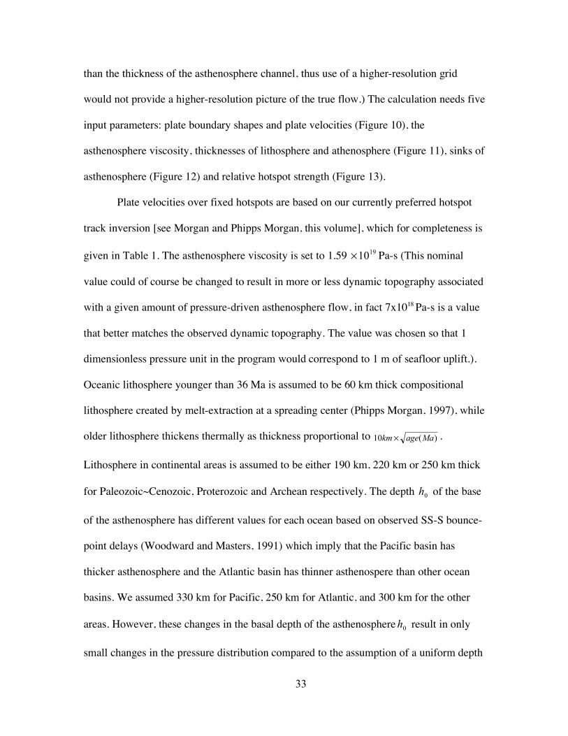
than the thickness of the asthenosphere channel, thus use of a higher-resolution grid

would not provide a higher-resolution picture of the true flow.) The calculation needs five

input parameters: plate boundary shapes and plate velocities (Figure 10), the

asthenosphere viscosity, thicknesses of lithosphere and athenosphere (Figure 11), sinks of

asthenosphere (Figure 12) and relative hotspot strength (Figure 13).

Plate velocities over fixed hotspots are based on our currently preferred hotspot

track inversion [see Morgan and Phipps Morgan, this volume], which for completeness is

given in Table 1. The asthenosphere viscosity is set to 1.59 1910! Pa-s (This nominal

value could of course be changed to result in more or less dynamic topography associated

with a given amount of pressure-driven asthenosphere flow, in fact 7x1018 Pa-s is a value

that better matches the observed dynamic topography. The value was chosen so that 1

dimensionless pressure unit in the program would correspond to 1 m of seafloor uplift.).

Oceanic lithosphere younger than 36 Ma is assumed to be 60 km thick compositional

lithosphere created by melt-extraction at a spreading center (Phipps Morgan, 1997), while

older lithosphere thickens thermally as thickness proportional to )(10 Maagekm ! .

Lithosphere in continental areas is assumed to be either 190 km, 220 km or 250 km thick

for Paleozoic~Cenozoic, Proterozoic and Archean respectively. The depth 0h of the base

of the asthenosphere has different values for each ocean based on observed SS-S bounce-

point delays (Woodward and Masters, 1991) which imply that the Pacific basin has

thicker asthenosphere and the Atlantic basin has thinner asthenospere than other ocean

basins. We assumed 330 km for Pacific, 250 km for Atlantic, and 300 km for the other

areas. However, these changes in the basal depth of the asthenosphere0h result in only

small changes in the pressure distribution compared to the assumption of a uniform depth

34

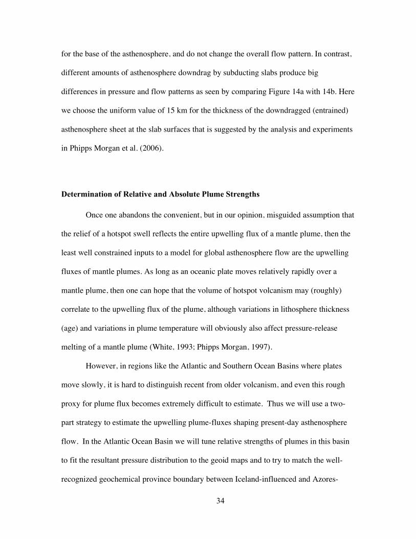
for the base of the asthenosphere, and do not change the overall flow pattern. In contrast,

different amounts of asthenosphere downdrag by subducting slabs produce big

differences in pressure and flow patterns as seen by comparing Figure 14a with 14b. Here

we choose the uniform value of 15 km for the thickness of the downdragged (entrained)

asthenosphere sheet at the slab surfaces that is suggested by the analysis and experiments

in Phipps Morgan et al. (2006).

Determination of Relative and Absolute Plume Strengths

Once one abandons the convenient, but in our opinion, misguided assumption that

the relief of a hotspot swell reflects the entire upwelling flux of a mantle plume, then the

least well constrained inputs to a model for global asthenosphere flow are the upwelling

fluxes of mantle plumes. As long as an oceanic plate moves relatively rapidly over a

mantle plume, then one can hope that the volume of hotspot volcanism may (roughly)

correlate to the upwelling flux of the plume, although variations in lithosphere thickness

(age) and variations in plume temperature will obviously also affect pressure-release

melting of a mantle plume (White, 1993; Phipps Morgan, 1997).

However, in regions like the Atlantic and Southern Ocean Basins where plates

move slowly, it is hard to distinguish recent from older volcanism, and even this rough

proxy for plume flux becomes extremely difficult to estimate. Thus we will use a two-

part strategy to estimate the upwelling plume-fluxes shaping present-day asthenosphere

flow. In the Atlantic Ocean Basin we will tune relative strengths of plumes in this basin

to fit the resultant pressure distribution to the geoid maps and to try to match the well-

recognized geochemical province boundary between Iceland-influenced and Azores-

35

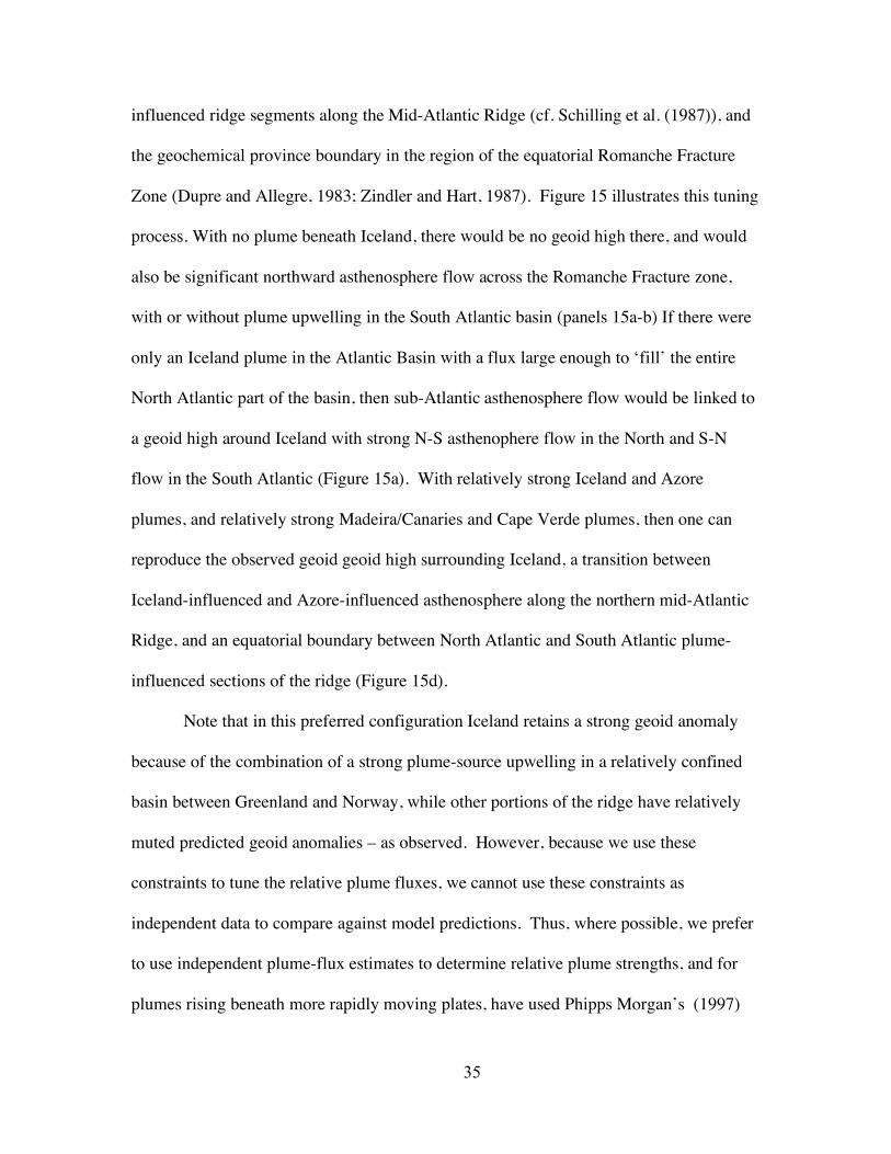
influenced ridge segments along the Mid-Atlantic Ridge (cf. Schilling et al. (1987)), and

the geochemical province boundary in the region of the equatorial Romanche Fracture

Zone (Dupre and Allegre, 1983; Zindler and Hart, 1987). Figure 15 illustrates this tuning

process. With no plume beneath Iceland, there would be no geoid high there, and would

also be significant northward asthenosphere flow across the Romanche Fracture zone,

with or without plume upwelling in the South Atlantic basin (panels 15a-b) If there were

only an Iceland plume in the Atlantic Basin with a flux large enough to ‘fill’ the entire

North Atlantic part of the basin, then sub-Atlantic asthenosphere flow would be linked to

a geoid high around Iceland with strong N-S asthenophere flow in the North and S-N

flow in the South Atlantic (Figure 15a). With relatively strong Iceland and Azore

plumes, and relatively strong Madeira/Canaries and Cape Verde plumes, then one can

reproduce the observed geoid geoid high surrounding Iceland, a transition between

Iceland-influenced and Azore-influenced asthenosphere along the northern mid-Atlantic

Ridge, and an equatorial boundary between North Atlantic and South Atlantic plume-

influenced sections of the ridge (Figure 15d).

Note that in this preferred configuration Iceland retains a strong geoid anomaly

because of the combination of a strong plume-source upwelling in a relatively confined

basin between Greenland and Norway, while other portions of the ridge have relatively

muted predicted geoid anomalies – as observed. However, because we use these

constraints to tune the relative plume fluxes, we cannot use these constraints as

independent data to compare against model predictions. Thus, where possible, we prefer

to use independent plume-flux estimates to determine relative plume strengths, and for

plumes rising beneath more rapidly moving plates, have used Phipps Morgan’s (1997)

36

and White’s (1993) estimates of hotspot magma production in the Pacific and Indian

Ocean Basins as a proxy for the relative strengths of plumes upwelling beneath these

basins. We are able to combine the Atlantic and rest of the world estimates of relative

plume strengths with the additional assumption that the total upwelling plume flux is

equal to the present-day rate of asthenosphere consumption, which we estimated (see

Figure 12) to be 406 km3/yr. Figure 14 and Table 2 show the plume strengths of our

preferred prediction of global asthenosphere flow.

Predicted Asthenosphere Flowfield & Pressure Distribution

Figure 16 shows the resulting global map of predicted asthenosphere flow. Strong

flow occurs beneath the Pacific Basin because of high plate speeds and strong ridgeward

fluxes from the equatorial Pacific ‘superswell’ region (McNutt and Fisher, 1987) and

Hawaii. In contrast, the Atlantic shows rather weaker asthenosphere flow because of its

much slower plate motions, smaller ridge-consumption of asthenosphere, and the

intermediate to weak strengths of its plumes. The Indian Ocean Basin exhibits strong

predicted asthenosphere flow in the Central Indian, with lesser flow rates in the north and

south. Note that the predicted pattern of asthenosphere ‘counterflow’ near subduction

zones ranges from parallel (cf. Tonga or Chile) to perpendicular (cf. NW Pacific

Trenches) to the nearest trench.

37

Tests of the predicted asthenosphere flowfield & pressure distribution

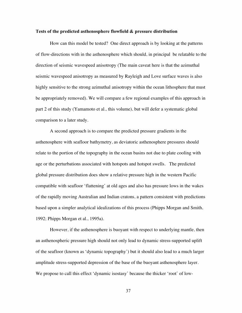
How can this model be tested? One direct approach is by looking at the patterns

of flow-directions with in the asthenosphere which should, in principal be relatable to the

direction of seismic wavespeed anisotropy (The main caveat here is that the azimuthal

seismic wavespeed anisotropy as measured by Rayleigh and Love surface waves is also

highly sensitive to the strong azimuthal anisotropy within the ocean lithosphere that must

be appropriately removed). We will compare a few regional examples of this approach in

part 2 of this study (Yamamoto et al., this volume), but will defer a systematic global

comparison to a later study.

A second approach is to compare the predicted pressure gradients in the

asthenosphere with seafloor bathymetry, as deviatoric asthenosphere pressures should

relate to the portion of the topography in the ocean basins not due to plate cooling with

age or the perturbations associated with hotspots and hotspot swells. The predicted

global pressure distribution does show a relative pressure high in the western Pacific

compatible with seafloor ‘flattening’ at old ages and also has pressure lows in the wakes

of the rapidly moving Australian and Indian cratons, a pattern consistent with predictions

based upon a simpler analytical idealizations of this process (Phipps Morgan and Smith,

1992; Phipps Morgan et al., 1995a).

However, if the asthenosphere is buoyant with respect to underlying mantle, then

an asthenospheric pressure high should not only lead to dynamic stress-supported uplift

of the seafloor (known as ‘dynamic topography’) but it should also lead to a much larger

amplitude stress-supported depression of the base of the buoyant asthenosphere layer.

We propose to call this effect ‘dynamic isostasy’ because the thicker ‘root’ of low-

38

density asthenosphere associated with the downward deflection of the base of the

asthenosphere beneath a region of high dynamic pressure is exactly the magnitude of the

deflection that would be predicted if one assumed that the dynamic seafloor uplift were

isostatically compensated by a thickened root of lower density asthenosphere. This mode

of compensation of a asthenospheric pressure gradient is the mode that maximizes

deformation into the low-viscosity asthenosphere layer while minimizing flow within the

underlying higher-viscosity mantle. The complexity it induces into a determination of

asthenospheric flow is that the depth of the asthenosphere channel becomes a function of

pressure. Since these initial calculations assume a fixed depth for the base of the

asthenosphere, their pressure prediction provide only a qualitative assessment of the

lateral pressure variations associated with asthenospheric flow. Since the asthenosphere’s

resistance to lateral flow depends upon the third power of the thickness of the

asthenospheric channel (eqn. 4), lateral pressure gradients will be reduced at pressure

highs where the asthenosphere is thickened by the effects of dynamic isostasy and will be

increased at pressure lows where the asthenosphere thins due to uplift of its base.

Furthermore, if the base of the buoyant asthenosphere is also compensating relief

associated with the deeper mantle flow associated with the flow-induced part of the

Geoid, then the thickness of the asthenosphere layer thickness should vary from this

effect, too. The calculated flow field is less sensitive to this second-order effect than is

pressure. Because of this, we focus on testing the predicted flow-field in this initial

determination of global asthenospheric flow, and defer a detailed exploration of the

predicted pressure field to a later study where we treat the effects of dynamic isostasy.

39

A third way is that regions of asthenosphere ‘fed’ by each hotspot can be

determined, and the boundaries between these regions should be evident at mid-ocean

ridges as geochemically distinct ‘provinces’ of mid-ocean ridge basalts. This third test is

the simplest to do now, as it takes advantage of the wealth of geochemical data that has

already been collected along the global ridge system. Thus this approach will be the

main focus of the following companion paper to this study (Yamamoto et al., this

volume). In the rest of this paper we will discuss other non-geochemical implications of

the asthenosphere flowfield predicted by this model, and then finish by noting current

limitations in our treatment of sub-continental plumes and the assumption of a steady-

state pattern of asthenosphere flow.

The Easter Island Vortex

One of the most curious features of the predicted pattern of asthenosphere flow

shown in Figure 16 occurs near the fastest-spreading part of the ridge spreading system

near Easter Island. A clear but small ‘vortex’ in the predicted flow pattern forms here as a

byproduct of the pattern of plate-spreading, and strengthened by the presence of the

nearby Foundation plume. (However, a weaker vortex pattern with the same spatial

pattern forms even when we remove the Foundation plume from the model, which shows

that the effect is primarily due to the pattern of plate spreading in this region.)

Two microplates, Easter and Juan Fernandez, are found in this fastest spreading

area. Schouten et al. (1993) proposed a microplate driving hypothesis they called the

“roller bearing” model. They suggested that a microplate rotates as a rigid block between

plates moving in opposite directions and presented analysis to dispute the hypothesis that

40

basal asthenospheric flow-induced shear stresses could be a significant driving force for

the observed internal rotation of microplates. Neves et al. (2003) tested the roller bearing

model with numerical experiments using the lithospheric stress pattern inferred from

observations at Easter microplate, and also concluded that asthenosphere flow could not

force microplate rotation, but instead should act as a resisting torque. They raised the

possibility of an asthenosphere vortex as a possible driving force, but discarded this

possibility on the grounds of its seemingly contrived geometry. However, given that our

predicted asthenosphere flow pattern shows a ‘helpful’ vortex in this region of microplate

activity, we speculate that the vortex may help force microplate rotation to some degree,

or at the very least make asthenosphere drag be much less of a rotation-resisting force.

This pattern also makes us wonder if the persistent creation of microplates may be an

indirect consequence of a persistant asthenosphere flow vortex beneath this region of the

spreading center.

Subcontinental plumes

Subcontinental plumes have been essentially ignored in this study, because we

consider that plume-fed asthenosphere will behave quite differently there than in the

suboceanic case. For example, seismic tomography shows very steep velocity gradients

around continental hotspots and low velocity zones form narrow corridors to points on the

boundary of continent and ocean (Ritsema and Allen, 2003). This suggests to us that a

pipe-like pattern of lateral plume-fed flow exists beneath continental lithosphere instead of

the flow pattern within a sheet of low-viscosity asthenosphere layer that exists beneath

ocean basins. We think the difference in flow pattern is related to the greater thickness of

41

continental lithosphere and the stronger lateral variations in the depth of the base of

continental tectosphere. As long as plume material is surrounded by more viscous mantle,

then its ability to form and flow within a low-viscosity conduit will dominate its flow

pattern. Only when a ‘pond or ‘puddle’ of low-viscosity asthenosphere has formed can

lateral asthenosphere flow be described by the equations discussed in this study. Thus we

imagine the drainage of asthenosphere from beneath continents to occur within ‘drainage’

channels of thinner tectosphere (i.e. beneath the relatively thinner lithosphere of ancient

sutures/failed rifts between cratons such as the Cameroon Line (Ebinger and Sleep, 1998)

For this initial study, we simply neglected the contribution of subcontinental hotspots, and

most regret the loss of a contribution from an Afar plume. In future work we hope to

merge this approach for suboceanic flow with a better characterization of subcontinental

plume-fed asthenosphere drainage through incorporation of the ‘upside-down drainage’

approach used by Sleep and coworkers.

Current limitations and future improvements

The predicted flow pattern shown in Figure 16 is based upon the assumption of

steady state. It assumes that the asthenosphere has had a steady state thickness, that the

plate geometry has not changed over time, that hotspot fluxes have remained constant

through time, and that the suboceanic viscosity is uniform throughout the asthenosphere

layer. We hope in future work to correct the oversimplification of a steady-state plate

geometry to include plate motion evolution, the opening of the continents and the

shrinkage of ocean basins, and to explore what impact secular changes in the thickness of

the asthenosphere have on predicted flow. With an iterative solution technique, one can

42

also improve the current neglect of the effects that ‘dynamic isostasy’ will have in

shaping the depth of the base of the asthenosphere, as discussed in the previous section.

We anticipate that a more realistic parameterization of these boundary conditions will

improve the model’s accuracy, at a cost of even greater model complexity. A further

possibility with this model is to estimate the plume flux distribution using additional

constraints from the observed directions of seismic anisotropy. We remain hopeful that

the asthenosphere flow modelling technique developed in the present study is a useful

tool to further test whether the paradigm of plume-hotspots and lateral flow within a

plume-fed asthenosphere can be reconciled with and provide a framework for

understanding the flow and melting of the upper mantle.

Acknowledgements. We would like to acknowledge Morgan A.L. Crooks, Jörg

Hasenclever, Walter Smith, and Mara Yale for their help during the 12 years of gestation

of this work. We also thank Don Anderson, Gill Foulger, Donna Jurdy, and Lars Rüpke

for helpful reviews.

43

REFERENCES CITED

(BVSP), B.V.S.P., 1981, Basaltic Volcanism on the Terrestrial Planets: New York,

Pergamon Press, 1286 p.

Abouchami, W., Galer, S.J.G., and Hofmann, A.W., 2000, High precision lead isotope

systematics of lavas from the Hawaiian Scientific Drilling Project: Chemical

Geology, v. 169, p. 187-209.

Abouchami, W., Hofmann, A.W., Galer, S.J.G., Frey, F.A., Eisele, J., and Feigenson, M.,

2005, Lead isotopes reveal bilateral asymmetry and vertical continuity in the

Hawaiian mantle plume: Nature, v. 434, p. 851-856.

Adam, C., and Bonneville, A., 2005, Extent of the South Pacific Superswell: J. Geophys.

Res., v. 110, p. doi:10.1029/2004JB3465.

Allegre, C.J., and Turcotte, D.L., 1986, Implications of a two-component marble-cake

mantle: Nature, v. 323, p. 123-127.

Anderson, D.L., 1989, Theory of the Earth, Blackwell Scientific, 366 p.

Bercovici, D., and Karato, S., 2003, Whole-mantle convection and the transition-zone

water filter: Nature, v. 425, p. 39-44.

Boyd, F.R., and McCallister, R.H., 1976, Densities of fertile and sterile garnet

peridotites: Geophys. Res. Lett., v. 3, p. 509-512.

Chase, C.G., 1979, Asthenospheric counterflow: A kinematic model: Geophys. J. R.

Astron. Soc., v. 56, p. 1-18.

Davies, G.F., 1988, Ocean bathymetry and mantle convection, 1, large-scale flow and

hotspots: J. Geophys. Res., v. 93, p. 10,467-10,480.

44

—, 1994, Thermomechanical erosion of the lithosphere by mantle plumes: J. Geophys.

Res., v. 99, p. 15709-15722.

—, 1999, Dynamic Earth, Cambridge University Press, 458 p.

Deffeyes, K.S., 1972, Plume convection with an upper mantle temperature inversion:

Nature, v. 240, p. 539-544.

Dupre, B., and Allegre, C.J., 1983, Pb-Sr isotope variation in Indian Ocean basalts and

mixing phenomena: Nature, v. 303, p. 142-146.

Dziewonski, A.M., and Anderson, D.L., 1981, Preliminary Earth Reference Model:

Physics of the Earth and Planetary Interiors, v. 25, p. 297-356.

Ebinger, C.J., and Sleep, N.H., 1998, Cenozoic magmatism throughout east Africa

resulting from impact of a single plume: Nature, v. 395, p. 788-791.

Ekstrom, G., and Dziewonski, A., 1998, The unique anisotropy of the Pacific upper

mantle: Nature, v. 394, p. 168-172.

Elsasser, W.M., 1971, Sea-floor spreading as thermal convection: J. Geophys. Res., v. 76,

p. 1101-1112.

Evans, R.L., Hirth, G., Baba, K., Forsyth, D.W., Chave, A., and Mackie, R., 2005,

Geophysical evidence from the MELT area for compositional controls on oceanic

plates: Nature, v. 437, p. 249-252.

Gaherty, J.B., Kato, M., and Jordan, T.H., 1999, Seismological structure of the upper

mantle: a regional comparison of seismic layering: Phys. Earth Planet Int., v. 110,

p. 21-41.

Gutenberg, B., 1959, Physics of the Earth's Interior, Academic Press, 240 p.

45

Harper, J.F., 1978, Asthenosphere flow and plate motions: Geophysical Journal Royal

Astronomical Society, v. 55, p. 87-110.

Hart, S.R., Hauri, E.H., Oschmann, L.A., and Whitehead, J.A., 1992, Mantle plumes and

entrainment: isotopic evidence: Science, v. 256, p. 517-520.

Hasenclever, J., 2004, Implications of a weak and buoyant asthenosphere for entrainment

and mantle flow at a subduction zone [Diplom thesis], IfM-GEOMAR, Kiel

University.

Helffrich, G.R., and Wood, B.J., 2001, The Earth's mantle: Nature, v. 412, p. 501-507.

Hess, P.C., 1989, Origins of Igneous Rocks: Cambridge, Harvard University Press, 336 p.

Hirth, G., and Kohlstedt, D.L., 1996, Water in the oceanic upper mantle: implications for

rheology, melt extraction, and the evolution of the lithosphere: Earth Planet. Sci.

Lett., v. 144, p. 93-108.

Hyndman, R.D., Currie, C.A., and Mazzotti, S.P., 2005, Subduction zone backarcs.

mobile belts, and orogenic heat: GSA Today, v. 15, p. 4-10.

Ito, G., and J., M., 2005a, Flow and melting of a heterogeneous mantle

2. Implications for a chemically nonlayered mantle: Earth and Planetary Science Letters,

v. 230, p. 47-63.

—, 2005b, Flow and melting of a heterogeneous mantle: 1. Method and importance to the

geochemistry of ocean island and mid-ocean ridge basalts: Earth and Planetary

Science Letters, v. 230, p. 29-46.

Jordan, T.H., 1979, Mineralogies, Densities, and Seismic Velocities of Garnet Lherzolites

and their Geophysical Implications, in Boyd, F.R., and Meyer, H.O.A., eds., Proc.

2nd Int. Kimberlite Conf., Vol. 2: Washington D. C., Am. Geophys. Union.

46

Karato, S., 1986, Does Partial Melting Reduce the Creep Strength of the Upper Mantle:

Nature, v. 319, p. 309-310.

Kumar, P., Kind, R., Hanka, W., Wylegalla, K., Reigber, C., Yuan, X., Woelnern, I.,

Schwintzer, P., Fleming, K., Dahl-Jensen, T., Larsen, T.B., Schweitzer, J.,

Priestley, K., Gudmundsson, O., and Wolf, D., 2005, The lithosphere-

asthenosphere boundary in the North-West Atlantic region: Earth Planet. Sci.

Lett., v. 236, p. 249-257.

Larson, R.L., 1991a, Geological consequences of super plumes: Geology, v. 19, p. 963-

966.

—, 1991b, Latest pulse of the Earth: Evidence for a mid-Cretaceous super plume:

Geology, v. 19, p. 547-550.

Larson, R.L., and Olson, P., 1991, Mantle plumes control magnetic reversal frequency:

Earth Planet. Sci. Lett., v. 107, p. 437-447.

Lee, C.-T., Lenardic, A., Cooper, C., Niu, F., and A., L., 2005, The role of chemical

boundary layers in regulating the thickness of continental and oceanic thermal

boundary layers: Earth Planet. Sci. Lett., v. 230, p. 379-395.

Lewis, T.J., Hyndman, R.D., and Flueck, P., 2003, Heat flow, heat generation, and crustal

temperatures in the northern Canadian Cordillera: Thermal control of tectonics: J.

Geophys. Res., v. 108, p. doi:10.1029/2002JB002090.

Li, X., Kind, R., Yuan, X., Woelbern, I., and Hanka, W., 2004, Rejuvenation of the

lithosphere by the Hawaiian plume: Nature, v. 427, p. 827-829.

47

McNutt, M.K., and Fischer, K.M., 1987, The South Pacific Superswell, in Keating, B.H.,

Fryer, P., Batiza, R., and Boehlert, G.W., eds., Seamounts, Islands, and Atolls,

Volume Geophysical Monograph #43, American Geophysical Union, p. 25-34.

Monnereau, M., Rabinowicz, M., and Arquis, E., 1993, Mechanical erosion and reheating

of the lithosphere: A numerical model for hotspot swells: J. Geophys. Res., v. 98,

p. 809-823.

Moore, W.B., Schubert, G., and Tackley, P., 1999, The role of rheology in lithospheric

thinning by mantle plumes: Geophys Res. Lett., v. 26, p. 1073-1076.

Morgan, W.J., 1971, Convection Plumes in the Lower Mantle: Nature, v. 230, p. 42.

—, 1972, Plate Motions and Deep Mantle Convection: Geol. Soc. Am. Memoir, v. 132,

p. 7-22.

—, 1981, Hotspot tracks and the opening of the Atlantic and Indian Oceans, in Emiliani,

C., ed., The Oceanic Lithosphere: New York, Wiley, p. 443-487.

Morgan, W.J., and Phipps Morgan, J., in press, Plate Velocities in the Hotspot Reference

Frame, in Foulger, G.R., and Jurdy, D., eds., Plates, Plumes, and Planetary

Processes: Geological Society of America Special Paper ###.

Nettles, M., 2005, Anisotropic velocity structure of the mantle beneath North America

[Ph.D. thesis]: Cambridge, Harvard.

Olson, P., 1990, Hot Spots, Swells, and Mantle Plumes, in Ryan, M.P., ed., Magma

Transport and Storage: New York, John Wiley, p. 33-51.

Oxburgh, E.R., and Parmentier, E.M., 1977, Compositional and Density Stratification in

Oceanic Lithosphere— Causes and Consequences: J. Geol. Soc. London, v. 133,

p. 343-355.

48

Parmentier, E.M., and Oliver, J.E., 1979, A study of shallow mantle flow due to the

accretion and subduction of lithospheric plates: Geophys. J. R. Astron. Soc., v. 57,

p. 1-22.

Phipps Morgan, J., 1987, Melt migration beneath mid-ocean spreading centers: Geophys.

Res. Lett., v. 14, p. 1238-1241.

—, 1994, The effect of mid-ocean ridge melting on subsequent off-axis hotspot upwelling

and melting: EOS Trans. AGU (Spring AGU Meeting Supplement), v. 75, p. 336.

—, 1997, The Generation of a Compositional Lithosphere by Mid-Ocean Ridge Melting

and its Effect on Subsequent Off-Axis Hotspot Upwelling and Melting: Earth

Planet. Sci. Lett., v. 146, p. 213-232.

—, 1998, Thermal and rare gas evolution of the mantle: Chem. Geol., v. 145, p. 431-445.

—, 1999, The isotope topology of individual hotspot basalt arrays: Mixing curves or melt

extraction trajectories?: Geochemistry, Geophysics, Geosystems, v. 1.

—, 2001, The thermodynamics of the pressure-release melting of a veined plum-pudding

mantle: Geochemistry, Geophysics, Geosystems, v. in press.

Phipps Morgan, J., and Connolly, J., 2004, Are MORB and OIB produced by a hybrid

flux-melting process instead of 'pure' pressure-release melting?: EOS Trans.

AGU, v. 85 Fall Meeting Supplement, p. Abstract V22A-08.

Phipps Morgan, J., Hasenclever, J., Hort, M., Rüpke, L., and Parmentier, E.M., 2006, On

subducting slab entrainment of buoyant asthenosphere: Terra Nova, v. in press.

Phipps Morgan, J., and Morgan, W.J., 1999, Two-stage melting and the geochemical

evolution of the mantle: a recipe for mantle plum-pudding: Earth Planet. Sci.

Lett., v. 170, p. 215-239.

49

Phipps Morgan, J., Morgan, W.J., and Price, E., 1995a, Hotspot melting generates both

hotspot volcanism and a hotspot swell?: J. Geophys. Res., v. 100, p. 8045-8062.

Phipps Morgan, J., Morgan, W.J., Zhang, Y.-S., and Smith, W.H.F., 1995b,

Observational hints for a plume-fed sub-oceanic asthenosphere and its role in

mantle convection: J. Geophys. Res., v. 100, p. 12753-12768.

Phipps Morgan, J., and Smith, W.H.F., 1992, Flattening of the seafloor depth-age curve

as a response to asthenospheric flow: Nature, v. 359, p. 524-527.

Ravine, M.A., 1997, Investigations into aspects of mantle viscosity and dynamics [Ph.D.

thesis]: San Diego.

Ravine, M.A., and Phipps Morgan, J., 1996, Inversion for radial mantle viscosity with a

layered constraint: A better fit to dynamic topography?: EOS Trans. AGU, v. 77,

p. F721.

Ritsema, J., and Allen, R., 2003, The elusive mantle plume: Earth Planet Sci. Lett., v.

207, p. 1-12.

Schilling, J.G., 1985, Upper mantle heterogeneities and dynamics: Nature, v. 314, p. 62-

67.

Schouten, H., Klitgord, K.D., and Gallo, D.G., 1993, Edge-driven microplate kinematics:

Journal of Geophysical Research, v. 98, p. 6689-6702.

Schubert, G., and Turcotte, D.L., 1972, One-dimensional model of shallow mantle

convection: J. Geophys. Res., v. 77, p. 945-951.

Schubert, G., Turcotte, D.L., and Olson, P., 2001, Mantle Convection in the Earth and

Planets, Cambridge University Press, 940 p.

50

Schubert, G., Yuen, D., Froidevaux, C., Fleitout, L., and Souriau, M., 1978, Mantle

circulation with partial shallow return flow: Effects on stresses in oceanic plates

and topography of the sea floor: J. Geophys. Res., v. 83, p. 745-758.

Sleep, N.H., 1984, Tapping of magmas from ubiquitous mantle heterogeneities: An

alternative to mantle plumes?: J. Geophys. Res., v. 89, p. 10029-10042.

—, 1990, Hotspots and Mantle Plumes: Some Phenomenology: J. Geophys. Res., v. 95,

p. 6715-6736.

ten Brink, U.S., and Brocher, T.M., 1987, Multichannel Seismic Evidence for a

Subcrustal Intrusive Complex Under Oahu and a Model for Hawaiian Volcanism:

J. Geophys. Res., v. 92, p. 13,687-13,707.

Turcotte, D.L., and Oxburgh, E.R., 1967, Finite amplitude convection cells and

continental drift: J. Fluid Mech., v. 28, p. 29-42.

White, R.S., 1993, Melt production rates in mantle plumes: Phil. Trans. Roy. Soc.

London A, v. 342, p. 137-153.

Yale, M.M., and Phipps Morgan, J., 1998, Asthenosphere flow model of hotspot-ridge

interactions: a comparison of Iceland and Kerguelen: Earth Planet. Sci. Lett., v.

161, p. 45-56.

Yamamoto, M., Phipps Morgan, J., and Morgan, W.J., in press, Global Plume-fed

Asthenosphere Flow: (2) Application to the Geochemical Segmentation of Mid-

Ocean Ridges, in Foulger, G.R., and Jurdy, D., eds., Plates, Plumes, and Planetary

Processes: Geological Society of America Special Paper ###.

Zindler, A., and Hart, S., 1986, Chemical Geodynamics: Annual Review of Earth and

Planetary Sciences, v. 14, p. 493-571.

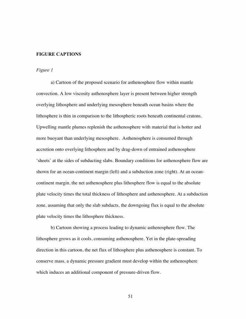
51

FIGURE CAPTIONS

Figure 1

a) Cartoon of the proposed scenario for asthenosphere flow within mantle

convection. A low viscosity asthenosphere layer is present between higher strength

overlying lithosphere and underlying mesosphere beneath ocean basins where the

lithosphere is thin in comparison to the lithospheric roots beneath continental cratons.

Upwelling mantle plumes replenish the asthenosphere with material that is hotter and

more buoyant than underlying mesosphere. Asthenosphere is consumed through

accretion onto overlying lithosphere and by drag-down of entrained asthenosphere

‘sheets’ at the sides of subducting slabs. Boundary conditions for asthenosphere flow are

shown for an ocean-continent margin (left) and a subduction zone (right). At an ocean-

continent margin, the net asthenosphere plus lithosphere flow is equal to the absolute

plate velocity times the total thickness of lithosphere and asthenosphere. At a subduction

zone, assuming that only the slab subducts, the downgoing flux is equal to the absolute

plate velocity times the lithosphere thickness.

b) Cartoon showing a process leading to dynamic asthenosphere flow. The

lithosphere grows as it cools, consuming asthenosphere. Yet in the plate-spreading

direction in this cartoon, the net flux of lithosphere plus asthenosphere is constant. To

conserve mass, a dynamic pressure gradient must develop within the asthenosphere

which induces an additional component of pressure-driven flow.

52

c) The asthenosphere sink due to slab drag-down. Lithosphere subducts dragging

a thin asthenosphere layer into mesosphere. In this study, the thickness d of the dragged

layer is set to 15km, following the boundary layer analysis in Phipps Morgan and Morgan

(1999) and the supporting lab and numerical experiments of Hasenclever (2004) and

Phipps Morgan et al. (2006).

Figure 2

Mean 1-D shear wave velocity structures over paths crossing the subcontinental

Australian craton (path AU3), suboceanic Philippine Sea backarc basin (path PHB3) and

suboceanic Pacific (PA5) upper mantle. Right panel shows the mean shear speeds for

each region, while the left panels show the anisotropic deviations about these means (in

all three cases, the vertical shear wavespeed VSV is slower than the horizontal shear

wavespeed VSH). Inset shows the map locations of the AU3, PHB3, and PA5 travel paths

resulting in each 1-D velocity model. (modified from Figure 4 of Gaherty et al., 1999).

Figure 3

Global shear wavespeed variations determined by M. Nettles using the approach

of Ekstrom and Dziewonski (1998) for depths of 70km, 100km, and150km. Variations in

isotropic shear wavespeed are shown at the top of each pair of maps, with anisotropic

variations from the isotropic average shown at the bottom. The isotropic shear

wavespeeds are shown with respect to the global average at each depth; no average has

been removed from the anisotropy maps (modified from Figure 5.4 of Meridith Nettles

Ph.D. thesis, Harvard, 2005).

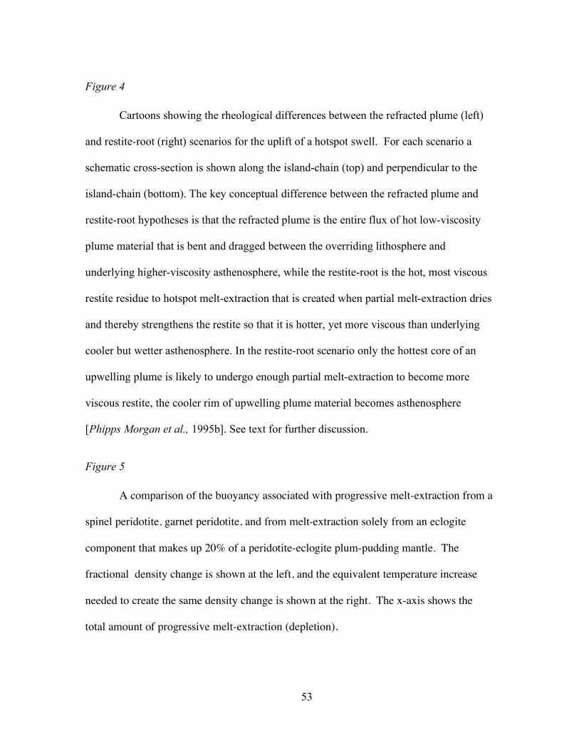
53

Figure 4

Cartoons showing the rheological differences between the refracted plume (left)

and restite-root (right) scenarios for the uplift of a hotspot swell. For each scenario a

schematic cross-section is shown along the island-chain (top) and perpendicular to the

island-chain (bottom). The key conceptual difference between the refracted plume and

restite-root hypotheses is that the refracted plume is the entire flux of hot low-viscosity

plume material that is bent and dragged between the overriding lithosphere and

underlying higher-viscosity asthenosphere, while the restite-root is the hot, most viscous

restite residue to hotspot melt-extraction that is created when partial melt-extraction dries

and thereby strengthens the restite so that it is hotter, yet more viscous than underlying

cooler but wetter asthenosphere. In the restite-root scenario only the hottest core of an

upwelling plume is likely to undergo enough partial melt-extraction to become more

viscous restite, the cooler rim of upwelling plume material becomes asthenosphere

[Phipps Morgan et al., 1995b]. See text for further discussion.

Figure 5

A comparison of the buoyancy associated with progressive melt-extraction from a

spinel peridotite, garnet peridotite, and from melt-extraction solely from an eclogite

component that makes up 20% of a peridotite-eclogite plum-pudding mantle. The

fractional density change is shown at the left, and the equivalent temperature increase

needed to create the same density change is shown at the right. The x-axis shows the

total amount of progressive melt-extraction (depletion).

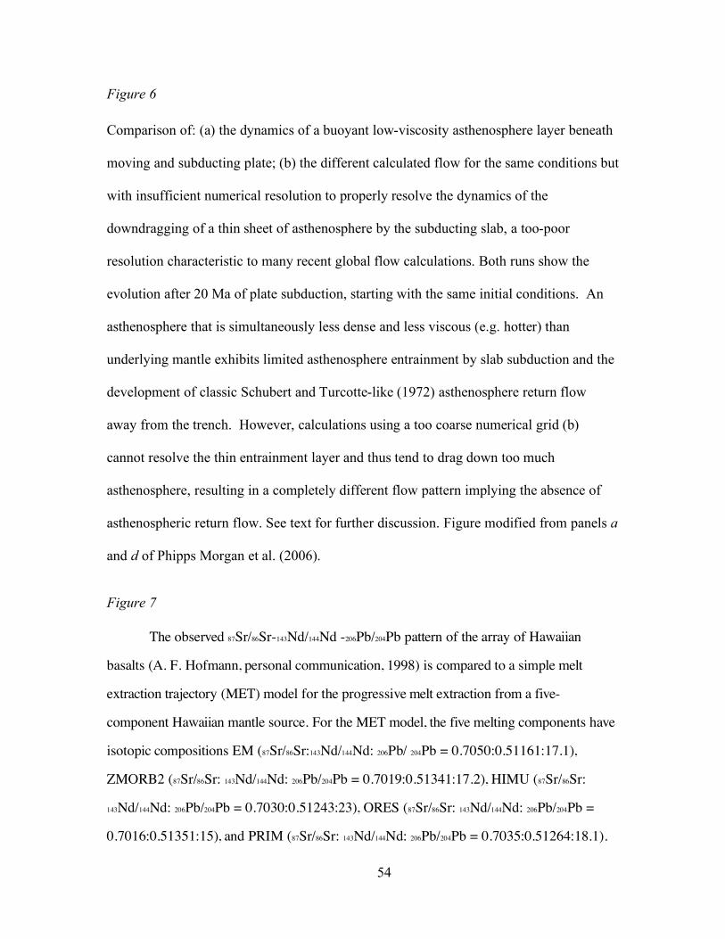
54

Figure 6

Comparison of: (a) the dynamics of a buoyant low-viscosity asthenosphere layer beneath

moving and subducting plate; (b) the different calculated flow for the same conditions but

with insufficient numerical resolution to properly resolve the dynamics of the

downdragging of a thin sheet of asthenosphere by the subducting slab, a too-poor

resolution characteristic to many recent global flow calculations. Both runs show the

evolution after 20 Ma of plate subduction, starting with the same initial conditions. An

asthenosphere that is simultaneously less dense and less viscous (e.g. hotter) than

underlying mantle exhibits limited asthenosphere entrainment by slab subduction and the

development of classic Schubert and Turcotte-like (1972) asthenosphere return flow

away from the trench. However, calculations using a too coarse numerical grid (b)

cannot resolve the thin entrainment layer and thus tend to drag down too much

asthenosphere, resulting in a completely different flow pattern implying the absence of

asthenospheric return flow. See text for further discussion. Figure modified from panels a

and d of Phipps Morgan et al. (2006).

Figure 7

The observed 87Sr/86Sr-143Nd/144Nd -206Pb/204Pb pattern of the array of Hawaiian

basalts (A. F. Hofmann, personal communication, 1998) is compared to a simple melt

extraction trajectory (MET) model for the progressive melt extraction from a five-

component Hawaiian mantle source. For the MET model, the five melting components have

isotopic compositions EM (87Sr/86Sr:143Nd/144Nd: 206Pb/ 204Pb = 0.7050:0.51161:17.1),

ZMORB2 (87Sr/86Sr: 143Nd/144Nd: 206Pb/204Pb = 0.7019:0.51341:17.2), HIMU (87Sr/86Sr:

143Nd/144Nd: 206Pb/204Pb = 0.7030:0.51243:23), ORES (87Sr/86Sr: 143Nd/144Nd: 206Pb/204Pb =

0.7016:0.51351:15), and PRIM (87Sr/86Sr: 143Nd/144Nd: 206Pb/204Pb = 0.7035:0.51264:18.1).

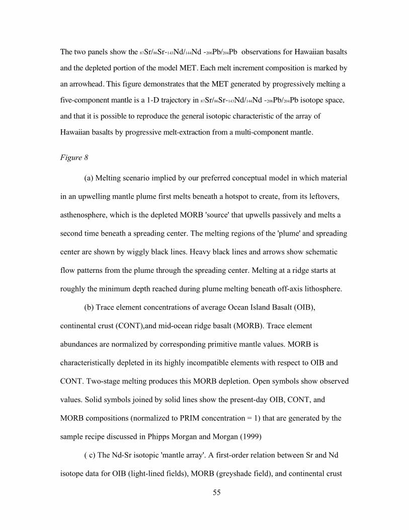
55

The two panels show the 87Sr/86Sr-143Nd/144Nd -206Pb/204Pb observations for Hawaiian basalts

and the depleted portion of the model MET. Each melt increment composition is marked by

an arrowhead. This figure demonstrates that the MET generated by progressively melting a

five-component mantle is a 1-D trajectory in 87Sr/86Sr-143Nd/144Nd -206Pb/204Pb isotope space,

and that it is possible to reproduce the general isotopic characteristic of the array of

Hawaiian basalts by progressive melt-extraction from a multi-component mantle.

Figure 8

(a) Melting scenario implied by our preferred conceptual model in which material

in an upwelling mantle plume first melts beneath a hotspot to create, from its leftovers,

asthenosphere, which is the depleted MORB 'source' that upwells passively and melts a

second time beneath a spreading center. The melting regions of the 'plume' and spreading

center are shown by wiggly black lines. Heavy black lines and arrows show schematic

flow patterns from the plume through the spreading center. Melting at a ridge starts at

roughly the minimum depth reached during plume melting beneath off-axis lithosphere.

(b) Trace element concentrations of average Ocean Island Basalt (OIB),

continental crust (CONT),and mid-ocean ridge basalt (MORB). Trace element

abundances are normalized by corresponding primitive mantle values. MORB is

characteristically depleted in its highly incompatible elements with respect to OIB and

CONT. Two-stage melting produces this MORB depletion. Open symbols show observed

values. Solid symbols joined by solid lines show the present-day OIB, CONT, and

MORB compositions (normalized to PRIM concentration = 1) that are generated by the

sample recipe discussed in Phipps Morgan and Morgan (1999)

( c) The Nd-Sr isotopic 'mantle array'. A first-order relation between Sr and Nd

isotope data for OIB (light-lined fields), MORB (greyshade field), and continental crust

56

(not shown) is that their Sr and Nd isotopic evolution is correlated, consistent with the

MORB coming from an isotopically depleted source. (Bulk-earth evolution is shown by

the PRIM hexagon.) Two stage melting of a plum-pudding mantle also produces

isotopically enriched OIB and isotopically depleted MORB (hexagons show present day

average OIB and MORB compositions that are generated by the recipe of Phipps Morgan

and Morgan (1999).) Figures taken from Phipps Morgan and Morgan (1999), where an

expansive description of this model is presented.

Figure 9

Cartoon showing our preferred view of how a plume-fed asthenosphere layer may

shape the large-scale structure of slab-subduction-driven mantle convection, and how this

flow pattern can be compatible with the observed geochemical differences between

hotspot (OIB) and mid-ocean ridge (MORB) basalts.

Figure 10

The absolute plate velocity model used as the lithosphere motion boundary

condition on asthenosphere flow. Table 1 gives Euler poles describing the absolute

velocity of each plate (The determinination of these absolute plate motions is presented in

Morgan and Phipps Morgan, this volume).

Figure 11

Map of lithosphere thicknesses used in this study. For oceanic lithosphere

younger than 36my a lithosphere thickness of 60 km is adopted, which is appropriate for

compositional lithosphere created by melt extraction at mid-ocean ridges (Phipps

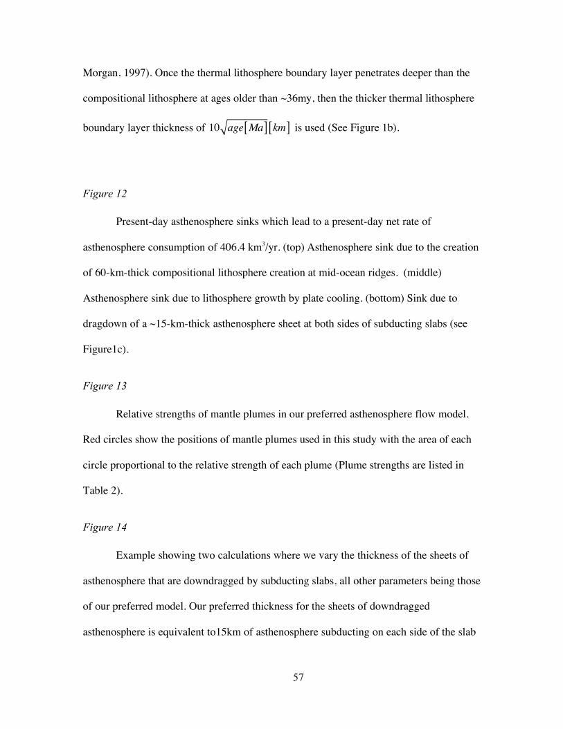
57

Morgan, 1997). Once the thermal lithosphere boundary layer penetrates deeper than the

compositional lithosphere at ages older than ~36my, then the thicker thermal lithosphere

boundary layer thickness of 10 age Ma[ ] km[ ] is used (See Figure 1b).

Figure 12

Present-day asthenosphere sinks which lead to a present-day net rate of

asthenosphere consumption of 406.4 km3/yr. (top) Asthenosphere sink due to the creation

of 60-km-thick compositional lithosphere creation at mid-ocean ridges. (middle)

Asthenosphere sink due to lithosphere growth by plate cooling. (bottom) Sink due to

dragdown of a ~15-km-thick asthenosphere sheet at both sides of subducting slabs (see

Figure1c).

Figure 13

Relative strengths of mantle plumes in our preferred asthenosphere flow model.

Red circles show the positions of mantle plumes used in this study with the area of each

circle proportional to the relative strength of each plume (Plume strengths are listed in

Table 2).

Figure 14

Example showing two calculations where we vary the thickness of the sheets of

asthenosphere that are downdragged by subducting slabs, all other parameters being those

of our preferred model. Our preferred thickness for the sheets of downdragged

asthenosphere is equivalent to15km of asthenosphere subducting on each side of the slab

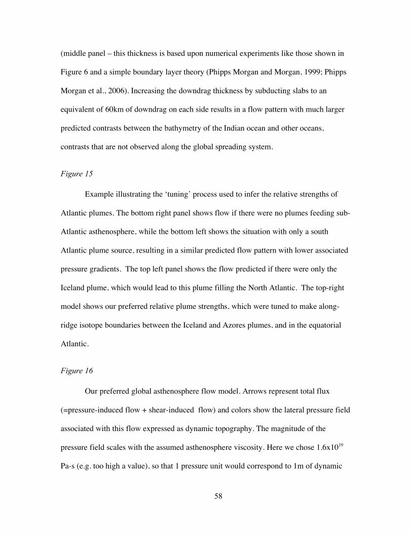
58

(middle panel – this thickness is based upon numerical experiments like those shown in

Figure 6 and a simple boundary layer theory (Phipps Morgan and Morgan, 1999; Phipps

Morgan et al., 2006). Increasing the downdrag thickness by subducting slabs to an

equivalent of 60km of downdrag on each side results in a flow pattern with much larger

predicted contrasts between the bathymetry of the Indian ocean and other oceans,

contrasts that are not observed along the global spreading system.

Figure 15

Example illustrating the ‘tuning’ process used to infer the relative strengths of

Atlantic plumes. The bottom right panel shows flow if there were no plumes feeding sub-

Atlantic asthenosphere, while the bottom left shows the situation with only a south

Atlantic plume source, resulting in a similar predicted flow pattern with lower associated

pressure gradients. The top left panel shows the flow predicted if there were only the

Iceland plume, which would lead to this plume filling the North Atlantic. The top-right

model shows our preferred relative plume strengths, which were tuned to make along-

ridge isotope boundaries between the Iceland and Azores plumes, and in the equatorial

Atlantic.

Figure 16

Our preferred global asthenosphere flow model. Arrows represent total flux

(=pressure-induced flow + shear-induced flow) and colors show the lateral pressure field

associated with this flow expressed as dynamic topography. The magnitude of the

pressure field scales with the assumed asthenosphere viscosity. Here we chose 1.6x1019

Pa-s (e.g. too high a value), so that 1 pressure unit would correspond to 1m of dynamic

59

topography. Our preferred value for the average viscosity of the asthenosphere would be

1/3-1/2 as large, which would produce ~1km of dynamic topography near the subduction

zones in the western Pacific. Note that this dynamic topography would be ‘compensated’

by opposing dynamic relief on the base of the asthenosphere, so that only a small Geoid

anomaly would be associated with this topography. (An example of this type of dynamic

isostasy is seen in the numerical experiment shown in Figure 6a).

TABLE 1. PLATE MOTIONS IN HOTSPOT-FIXED FRAME Plate Latitude

(°N) Longitude

(°E) Angular rate

(°/my) Max speed

(mm/yr) Africa 43.07 -24.56 0.1544 17.16 Antarctica 70.18 82.26 0.0989 10.99 Arabia 31.00 13.06 0.5205 57.83 Australia 20.14 40.28 0.6990 77.67 Caribbean -20.80 -56.84 0.0808 8.98 Cocos 22.32 -116.24 1.3343 148.26 Eurasia 82.54 -125.53 0.0619 6.88 Juan de Fuca -31.32 60.04 0.8540 94.89 Nazca 49.95 -95.74 0.5634 62.60 North America -51.87 -48.70 0.1628 18.08 Pacific -59.33 94.90 0.8028 89.20 Philippine -45.71 -23.83 0.9928 110.31 South America -75.22 100.24 0.1749 19.43

Note: Values from Morgan and Phipps Morgan, this volume

TABLE 2. HOTSPOT/PLUME LOCATIONS & STRENGTHS Hotspot Latitude

(°N) Longitude

(°E) Strength

(see note) Iceland 64.4 -17.3 0.60 Azores 37.9 -26.0 0.40 Bermuda 32.4 -64.0 0.08 Madeira 32.7 -17.0 0.00 Canary 28.2 -18.0 0.15 GreatMeteor 29.4 -29.2 0.05 CapeVerde 14.9 -24.3 0.40 Cameroon -2.0 5.1 0.30 FernandoDoNorono -4.0 -32.3 0.08 Ascension -7.9 -14.3 0.10 StHelena -15.6 -7.0 0.30 MartinVaz -20.5 -28.9 0.08 Vema -32.1 6.3 0.15 TristanDaCunha -37.2 -12.3 0.25 Gough -40.3 -10.0 0.36 Discovery -43.0 -2.7 0.20 Bouvet -51.4 1.1 0.35 Ob-Lena -52.2 40.0 0.40 Marion -46.9 37.6 0.40 Crozet -26.1 50.2 0.40 Kerguelen -49.6 69.0 0.50 Heard -53.1 73.5 0.10 Reunion -21.2 55.7 0.60 Comores -11.5 43.3 0.15 LordHowe -34.7 159.8 0.10 Tasmantid -40.4 155.5 0.15 EasternAustralia -40.8 146.0 0.15 Cocos-Keeling -17.0 94.5 0.05 Caroline 4.8 156.4 0.10 Hawaii 19.1 -155.1 2.00 Samoa -14.6 -168.2 0.80 Marquesas -10.5 -139.0 0.80 Society -17.9 -148.2 0.80 Macdonald -29.0 -140.3 0.20 Line -27.0 -139.0 0.10 Pitcairn -25.2 -129.1 0.10 Louisville -50.9 -138.1 0.25 Foundation -37.0 -113.0 0.35 Easter -26.8 -107.6 0.10 Galapagos -0.4 -91.6 1.30 JuanFernandez -33.9 -81.8 0.40 SanFelix -26.4 -80.1 0.05 Guadalupe 26.8 -112.4 0.10 Cobb 46.2 -130.0 0.10 Bowie 53.3 -135.7 0.10 Scott -68.8 -178.0 0.05 Peter-I -68.8 -90.7 0.01 Gaussberg -66.8 89.3 0.05 Balleny -67.6 164.8 0.05 Note: A plume strength of 1 corresponds to an upwelling plume flux of 29.4km3/yr; implying a total plume upwelling flux

of 406 km3/yr.

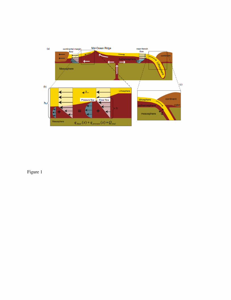
Figure 1

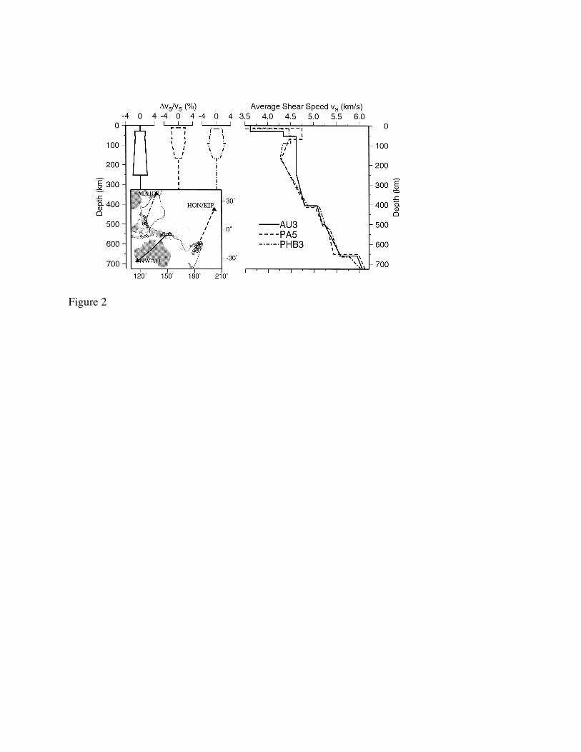
Figure 2

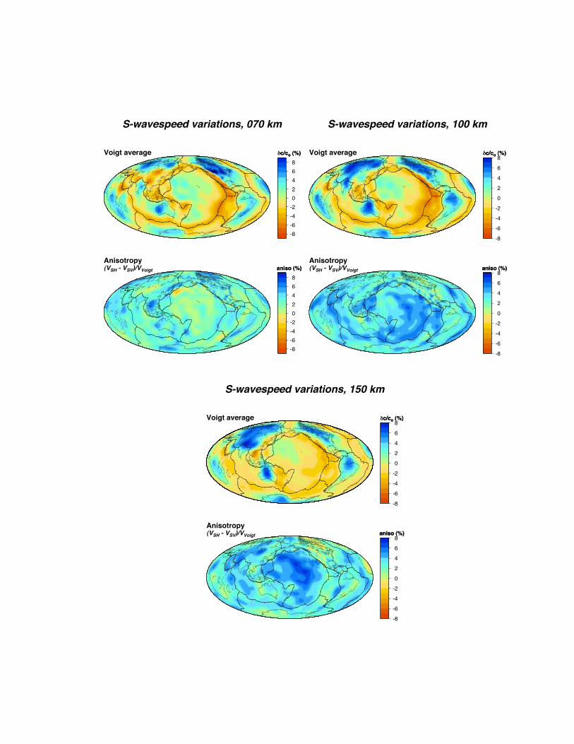
S-wavespeed variations, 070 km

Voigt average

Anisotropy(VSH - VSV)/VVoigt

δc/co (%)δc/co (%)

aniso (%)aniso (%)

-8-6-4-202468

-8-6-4-202468

S-wavespeed variations, 100 km

Voigt average

Anisotropy(VSH - VSV)/VVoigt

δc/co (%)δc/co (%)

aniso (%)aniso (%)

-8

-6

-4

-2

0

2

4

6

8

-8

-6

-4

-2

0

2

4

6

8

S-wavespeed variations, 150 km

Voigt average

Anisotropy(VSH - VSV)/VVoigt

δc/co (%)δc/co (%)

aniso (%)aniso (%)

-8

-6

-4

-2

0

2

4

6

8

-8

-6

-4

-2

0

2

4

6

8

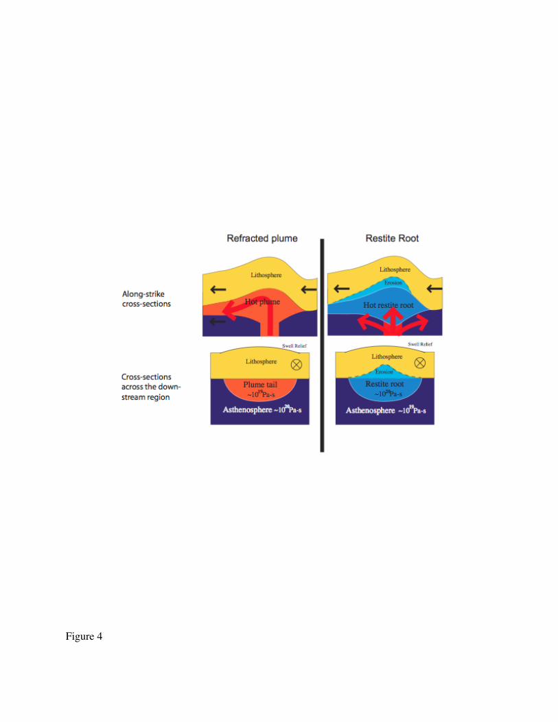
Figure 4

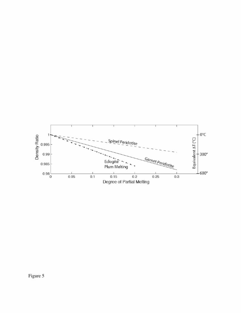
Figure 5

b)

a)

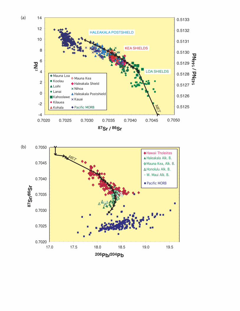
-4

-2

0

2

4

6

8

10

12

14

0.7020 0.7025 0.7030 0.7035 0.7040 0.7045 0.7050

87Sr / 86Sr

KEA SHIELDS

LOA SHIELDS

HALEAKALA POSTSHIELD

Mauna LoaKoolauLoihiLanaiKahoolaweKilaueaKohala

Mauna KeaHaleakala Shield

Pacific MORB

Kauai

NihoaHaleakala Postshield

εNd

0.5125

0.5126

0.5127

0.5128

0.5129

0.5130

0.5131

0.5132

0.5133

143 N

d / 1

44N

d

MET

(a)

(b)

17.5 18.0 18.5 19.0 19.5

Hawaii Tholeiites

Pacific MORB

Haleakala Alk. B.Mauna Kea, Alk. B.Honolulu Alk. B.W. Maui Alk. B.

0.7020

0.7025

0.7030

0.7035

0.7040

0.7045

0.7050

17.0206Pb/204Pb

87Sr

/86Sr

MET

Nd-Sr ‘Mantle Array’(c)(b)

(a) Two-Stage Plume-Ridge Melting

asthenosphereZP

ZR

Restite

Crust

ThermalLithosphere

mesosphere

MeltingZone

MeltingZone

Upwelling Mantle Plume

OIB MORB

Figure 9

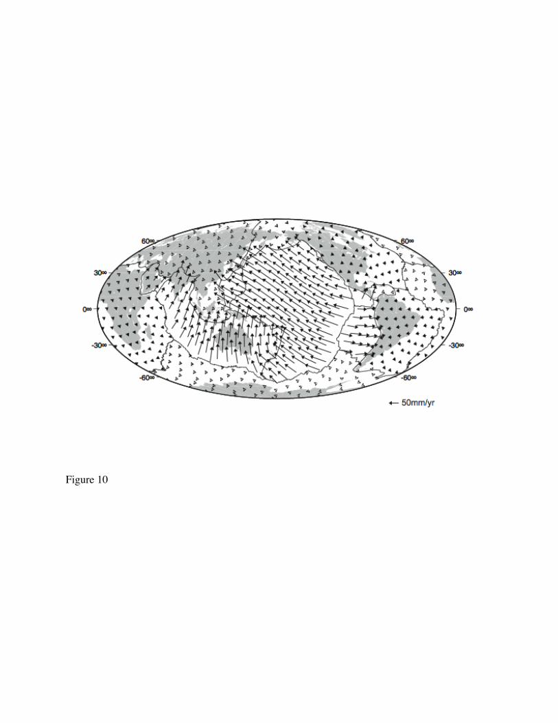
Figure 10

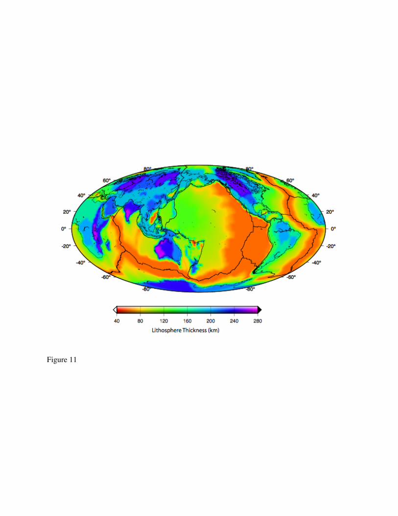
Figure 11

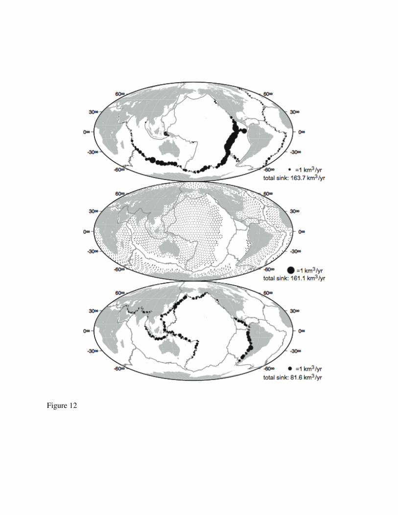
Figure 12

Figure 13

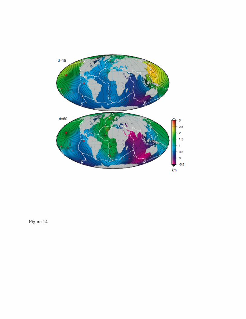
Figure 14

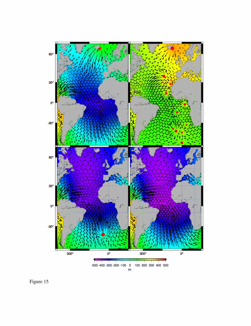
Figure 15

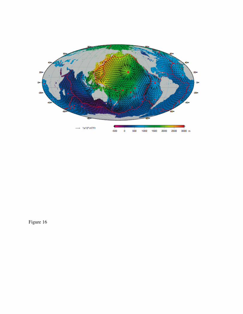
Figure 16