Estimation of Loss Given Default for Low Default Portfolios · 2.4 The mathematical nature of Loss Given Default ... 6.3 Test results ... can be a support for business decisions

Estimation of Loss Given Default for Low Default Portfolios

Fredrik Dahlin Samuel Storkitt Royal Institute of Technology Stockholm, Sweden 2014

Estimation of Loss Given Default for Low Default Portfolios 2014

1

ABSTRACT The Basel framework allows banks to assess their credit risk by using their own estimates of Loss Given Default (LGD).

However, for a Low Default Portfolio (LDP), estimating LGD is difficult due to shortage of default data. This study evaluates

different LGD estimation approaches in an LDP setting by using pooled industry data obtained from a subset of the PECDC

LGD database. Based on the characteristics of a LDP a Workout LGD approach is suggested. Six estimation techniques,

including OLS regression, Ridge regression, two techniques combining logistic regressions with OLS regressions and two tree

models, are tested. All tested models give similar error levels when tested against the data but the tree models might produce

rather different estimates for specific exposures compared to the other models. Using historical averages yield worse results

than the tested models within and out of sample but are not considerably worse out of time.


2

LIST OF FIGURES

Figure 1. Illustration of sample space

Figure 2. Number of observations over time

Figure 3. Empirical LGD distribution Figure 4. Trend component in German long term interest rate

Figure 5. UK 1Y stock market returns

Figure 6. Proportion of nominal LGD equal to zero Figure 7. Regression tree based on original LGD observations

Figure 8. Regression tree based on adjusted LGD observations

Figure 9. F-tree based on original LGD observations

Figure 10. F-tree based on adjusted LGD observations


3

LIST OF TABLES

Table 1. Workout and Market LGD estimation techniques

Table 2. Identification problem remedies

Table 3. Time to resolution Table 4. Country of jurisdiction for financial institutions

Table 5. Subsets for out of time testing

Table 6. Macroeconomic variables in OLS regression Table 7. Bank and non-banks with nominal LGD equal to zero

Table 8. Splitting year into dummy variable

Table 9. OLS regression results

Table 10. Ridge regression results

Table 11. Logistic-OLS Regressions results

Table 12. Trimmed Logistic-OLS Regressions results Table 13. Predictive power for original LGD levels

Table 14. Predictive power for adjusted LGD levels

Table 15. Splitting continuous variables (illustrative graph) Table 16. LGD estimates

Table 17. Exposures in Table 16

Table 18. LGD distribution for example portfolio Table 19. LGD percentiles for example portfolio

Table 20. Correlation matrix of LGD estimates in example portfolio


4

LIST OF ABBREVIATIONS

A-IRB Advanced Internal Rating Based

F-IRB Foundation Internal Rating Based

EAD Exposure At Default EL Expected Loss

IRB Internal Rating Based

LDP Low Default Portfolio LGD Loss Given Default

PD Probability of Default

PIT Point In Time

SDR Standard Deviation Reduction

SME Small and Medium Enterprises

TTC Through The Cycle UL Unexpected Loss

VaR Value at Risk

Models FT F-Tree (introduced in this paper) LR-OLS Logistic-OLS Regressions (introduced in this paper)

OLS Ordinary Least Squares regression

RiR Ridge Regression

RT Regression Tree

TLR-OLS Trimmed Logistic-OLS Regression (introduced in this paper)

Hist Historical average

Model evaluation methods MAE Mean Absolute Error ME Mean Error

R2 R-squared value


5

TABLE OF CONTENTS Abstract ................................................................................................................................................................................................. 1 List of figures ........................................................................................................................................................................................ 2 List of tables ......................................................................................................................................................................................... 3 List of abbreviations ............................................................................................................................................................................. 4 1 Introduction ................................................................................................................................................................................. 6 2 Theoretical background .............................................................................................................................................................. 8

2.1 Definition of default ............................................................................................................................................................... 8 2.2 Definition of Loss Given Default (LGD) ................................................................................................................................ 8 2.3 Definition of Low Default Portfolio (LDP) .............................................................................................................................. 9 2.4 The mathematical nature of Loss Given Default (LGD) ....................................................................................................... 9 2.5 The Low Default Portfolio (LDP) problem ..........................................................................................................................10 2.6 Point in time, through the cycle and downturn estimates ..................................................................................................11 2.7 LGD estimation approaches ...............................................................................................................................................11 2.8 LGD estimation approaches for LDPs ................................................................................................................................13 2.9 What affects LGD? (Risk drivers) .......................................................................................................................................13

3 Models ......................................................................................................................................................................................17 4 Data ..........................................................................................................................................................................................20 5 Model evaluation methods .......................................................................................................................................................23 6 Results ......................................................................................................................................................................................25

6.1 Risk drivers ..........................................................................................................................................................................25 6.2 Final models ........................................................................................................................................................................31 6.3 Test results ..........................................................................................................................................................................34 6.4 Summary of results .............................................................................................................................................................38

7 Concluding remarks..................................................................................................................................................................40 8 References ...............................................................................................................................................................................41


6

1 INTRODUCTION A sound and stable financial system is an essential part of a growing and prosperous society. In contrast, a financial crisis can

severely damage the economic output of a society for an extended period of time, as seen in recent years. In order to reduce

the risk of future crises, banks and other financial institutions are regulated. The outlines of banking regulations are set in the

Basel accords, where banks are deemed to have a certain amount of capital in order to cover potential future losses.

The risks facing banks are multifaceted and therefore divided into several parts, the main ones being credit risk, market risk

and operational risk. In order to assess the credit risk, certain risk parameters must be estimated. These include Probability of

Default (PD), Loss Given Default (LGD) and Exposure At Default (EAD). The Basel framework defines three possible

approaches for assessing the credit risk exposure. The Standardized approach, the Foundation Internal Rating Based approach

(F-IRB) and the Advanced Internal Rating Based approach (A-IRB). Differing to the standardized and F-IRB approach, the A-

IRB approach requires the bank to use its own estimates of LGD and EAD in addition to PD. In the standardized and F-IRB

approach the LGD parameter is given by the regulators. This thesis focuses on the estimation of LGD. Historically, a lot of

focus has been devoted to the estimation of PD while LGD has received less attention and has sometimes been treated as

constant. Das and Hanouna (2008) note that using constant loss estimates might be misleading since losses experience large

variation in reality. According to Moody’s (2005) average recovery rates, defined as 1- LGD, can vary between 8% and 74%

depending on the year and the bond type. For a sophisticated risk management, LGD clearly needs to be assessed in more

detail.

The estimation of LGD is preferably conducted by using historical loss data, but for certain portfolios and counterparties, there

is a shortage of such data due to the high quality of the assets and the low number of historical defaults. Portfolios of this kind

are often referred to as Low Default Portfolios (LDPs). LDPs include portfolios with exposures to e.g. banks, sovereigns and

highly rated corporations. The most extreme examples include covered bonds with very few cases where a loss has occurred.

For LDPs the estimation of credit risk parameters like LGD is problematic and this has led to questions from the industry

concerning how to handle these portfolios.

The purpose of this thesis is to study quantitative models for estimation of LGD and empirically evaluate how these models

work on LDPs in order to find a model that can be used in practice. For the model to be useful in practice it must produce

reasonable and justifiable values despite little default data. While the models are based solely on quantitative factors also

qualitative considerations are taken into account when the models are constructed.

The outcome of the study will constitute of two parts, the first being an overview of the academic progress in this area and the

second an evaluation of models from a practical perspective. The direct beneficiaries of the thesis are banks and financial

institutions with the need to assess their credit risk exposure.

The benefit of a better credit risk assessment is twofold. First it gives banks a better control over the risks they are facing and

can be a support for business decisions. Secondly, internal models typically results in lower risk measures and thereby lower

capital requirements. Since capital is costly, this is a direct benefit for a bank. On a more general level, society as a whole

benefits from sound financial institutions with good credit risk assessments.

The remainder of this report is structured as follows. Chapter 2 presents a theoretical background to LGD and LDPs. In

Chapter 3 the models used in this study are presented. Chapter 4 gives an overview of the data used for this study while


7

Chapter 5 presents the evaluation methods used. In Chapter 6 the results are presented and Chapter 7 contains concluding

remarks.


8

2 THEORETICAL BACKGROUND

2.1 DEFINITION OF DEFAULT The event of default can be defined in many ways and it differs for different purposes and disciplines. A default from a legal

point of view is not necessarily the same as a default from an economic point of view. For the purpose of this paper it is

important that the definition

1) Complies with relevant regulations

2) Is consistent with the definition used to estimate the probability of default parameter (PD)

For these reasons we use the definition communicated in the Basel framework (BIS, 2006, § 452)

A default is considered to have occurred with regard to a particular obligor when either or both of the two following events have taken place.

- The bank considers that the obligor is unlikely to pay its credit obligations to the banking group in full, without recourse by the bank to actions such as realising security (if held).

- The obligor is past due more than 90 days on any material credit obligation to the banking group. Overdrafts will be considered as being past due once the customer has breached an advised limit or been advised of a limit smaller than current outstandings.

When this definition is used a default occurs when the obligor is unlikely to pay or is late with a payment. As the obligor does

not necessarily have to miss a payment for a default to occur it is not impossible that the obligor will actually pay the full

amount on time and the loss be equal to zero.

2.2 DEFINITION OF LOSS GIVEN DEFAULT (LGD) LGD is the economic loss occurring when an obligor defaults. It is expressed in percentage of the defaulted amount. The

defaulted amount is equal to the principal amount and overdue interest payments. This is consistent with the finding of

Andritzky (2005) that the core legal claim consists of the nominal value and is often referred to as the recovery of face value

assumption. In accordance with the Basel framework the LGD estimates are based on the economic loss and include workout

costs arising from collecting the exposure (BIS, 2006, § 460). These costs are included in the modelled LGD since it is believed

that they are affected by the exposure type. Complicated bankruptcy processes might imply a larger use of external lawyers for

instance. Since workout costs are included, the LGD value can be larger than one. However, since this is not believed to occur

frequently, LGD is assumed to be equal to or lower than one and LGD observations and estimates are therefore capped at one.

The cash flows received during the workout process are adjusted with a discount rate equal to the risk free interest rate at the

time of default. The use of the risk free interest rate for calculating the present value of the cash flows is a simplification. In

practice regulators require the discount rate to include an appropriate risk premium (BIS 2005a). However, there is no

consensus among practitioners and banking supervisors regarding what discount rate to apply for different cases (Brady et al

2006). Since the addition of a risk premium is not believed to affect the choice of a model it is not considered in this study.


9

2.3 DEFINITION OF LOW DEFAULT PORTFOLIO (LDP) There is no exact definition of a LDP accepted by the industry (BIS, 2005b). Instead, the Basel Committee Accord

Implementation Group’s Validation Subgroup points out that a bank’s portfolio is not either low default or non-low default but

that there is “a continuum between these extremes” and notes that “a portfolio is closer to the LDP end of this continuum when a

bank’s internal data systems include fewer loss events, which presents challenges for risk quantification and validation” (BIS,

2005b § 1).

The International Swaps and Derivatives Association (ISDA) notes in a joint working paper (2005) that examples of LDPs

include e.g. exposures to sovereigns, banks, large corporates and repurchase agreements (ISDA, 2005).

2.4 THE MATHEMATICAL NATURE OF LOSS GIVEN DEFAULT (LGD) LGD is the loss conditional upon the event of default. The parameter depends therefore crucially on the default definition. While

the definition varies for different purposes and disciplines this paper use the definition from the Basel accords, see Section 2.1.

The definitions of LGD and the default event have two important implications.

1) Only losses of cash flows (principal and overdue interest payments and workout costs) are considered. Losses purely

due to market movements or a changed market price of the underlying are not considered.

2) A loss cannot occur without the event of default since a loss of a principal or interest payment necessarily leads to

the state of default.

Considering a probability space two random variables can be defined:

[ ] .

Loss given default can then be defined as the random variable G .

Furthermore three important outcomes can be identified:

It should be noted that due to the definitions of loss and default the following holds for the loss variable

( )

This leaves the case when .

Equation (1) highlights the importance of a consistent default definition for the PD and LGD parameters since the PD parameter

is in fact part of the LGD random variable. PD is defined as P(D=1) in

Ω A

B C

Figure 1. Illustration of sample space


10

( ) ( ) ( )

( )

( )

( )

The input to the credit risk reporting will be the expected value of the random variable LGD,

[ ]

Contrary to the mathematics derived in this paper regulators require the LGD parameter to be a “downturn G ” reflecting the

LGD in a downturn environment and not the expected value of the random variable. The Basel committee suggests two ways

of deriving a downturn LGD. One could either use a mapping function to extrapolate the normal LGD or one could provide a

separate downturn LGD estimate.

2.5 THE LOW DEFAULT PORTFOLIO (LDP) PROBLEM LDPs are not mentioned explicitly in the Basel II framework (Kofman, 2011) but portfolios of this kind have raised concerns

from the industry, fearing that these portfolios might end up excluded from IRB-treatment. The Basel committee has

acknowledged these concerns and stated in a newsletter in 2005 that LDPs should not automatically be excluded from IRB-

treatment. The committee suggested some remedies for the shortage of data including pooling of loss data and combination of

portfolios with similar characteristics (BIS, 2005b). However, no models or solutions are proposed if the problem persists.

Most studies concerning the estimation problems for LDPs are focusing on the problem of estimating the probability of default

parameter even though the LDP problem may be even more severe for LGD estimation. ISDA (2005) notes that there

sometimes might exist a sufficient amount of defaults to estimate PD but too few observations to estimate LGD. Kofman (2011)

suggests that LDPs may be extended by “near defaults” (called “quasi-defaults”) with a similar financial profile in order to

overcome the issue of too little data. A near default might be identified by a high risk profile or a low/downgraded credit rating.

While this might be helpful for the estimation of PD it seems unlikely that it would improve the LGD estimation since these

observations per definition has a loss of zero. Other proposed ways of estimating PD includes for instance the use of migration

matrices and Markov Chains. In these models migration rates between rating grades are used in order to assess the likelihood

of a highly rated asset to be downgraded and eventually defaulted (Schuermann and Hanson, 2004). This approach requires

default data for lower rating grades and might therefore not be applicable when there are a low number of defaults in the whole

portfolio. Furthermore, even if there is some evidence that rating grades do affect the recovery rates (Altman et al., 2004) it is

hard to see how to extend the data for LGD in the same way as for PD estimations.

Pluto and Tachse (2005) present a model using the “most prudent estimation” principle that does not share the requirement of

defaults for lower rating grades. Their model assumes that the initial ranking is correct and an asset with a lower rating cannot

have a lower probability of default than an asset with a higher rating. They derive confidence intervals for the probability of

default for every rating grade based on the number of defaults and PD parameters are estimated as the upper confidence

bounds. This guarantees that the differences between the credit ratings are preserved. A disadvantage of the model is the

prerequisite of a ranking system. Furthermore, while the use of ratings might be sensible for estimating PD this might not be

appropriate for the estimation of LGD.

While the LDP problem affects all components of the expected loss (PD, LGD and EAD) most focus has so far been on the

estimation of PD. Apart from pooling of data, suggested remedies are unfortunately not applicable on LGD estimation.


11

2.6 POINT IN TIME, THROUGH THE CYCLE AND DOWNTURN ESTIMATES There are two main approaches used when defining parameters for risk estimation, Point in Time (PIT) and Through the Cycle

(TTC). A PIT estimate is constructed to capture the risk at every point in time while a TTC estimate is constructed to capture

the average risk through a business cycle. This study aims to provide a TTC estimate and discuss the inclusion of

macroeconomic variables only as a way of generating the downturn estimate required by regulators.

PECDC (2013a) notes that observations of defaulted banks and financial institutions are typically connected to crises and LGD

estimates for banks and financial institutions are therefore already associated with downturns in the financial markets. It can

therefore be questioned to what degree separate downturn LGD estimates have to be produced for this particular type of

exposures. Looking at the sample in this study, more than half of the data is associated with downturn periods.

2.7 LGD ESTIMATION APPROACHES As CEBS (2006) does not suggest a specific model or approach for LGD estimation but merely concludes that “supervisors do

not require any specific technique for G estimation” (p. 72) the choice of method is an important part of G estimation.

CEBS (2006) lists four main techniques for quantitative estimation of LGD. These are Workout LGD, Market LGD, Implied

Market LGD and Implied Historical LGD. Workout LGD is estimated from cash flows from the workout process and Market LGD

estimates are derived from the prices of defaulted bonds. Implied Market LGD is instead derived from the prices of non-

defaulted bonds or derivatives on said bonds and could thus be used to estimate the LGD without the security actually

defaulting. However, CEBS (2006) points out that Market LGD and Implied Market LGD only can be used in limited

circumstances and probably not for the main part of a loan portfolio. Implied Historical LGD is only allowed for retail exposures

and hence cannot be applied for the purpose in this study.

WORKOUT AND MARKET LGD The choice between Workout and Market LGD is essentially the choice of when to observe the recovery rate. Workout LGD

estimations use ultimate recoveries from the workout process while Market LGD estimations use the trading prices at some

time after default. The advantage of the Workout LGD procedure is that it uses the true values of recoveries while Market LGD,

affected by the supply and demand, risk aversion and liquidity of the post-default market, has been found to systematically

underestimate the true recovery rates (Renault and Scaillet, 2004). A Market LGD estimation also requires that the defaulted

security is actually traded on a public market. However, using Market LGD makes it possible to include defaults that occurred

recently in the model. As a workout processes can last several years (Araten, 2004) this is a considerable advantage when

data is scarce. Table 1 lists possible approaches for the estimation of LGD using observed Workout or Market LGD.


12

Estimation techniques

Parametric:

Ordinary least squares regression (OLS) (e.g. Qi and Zhao, 2012)

Ridge regression (RiR) (Loterman, 2012)

Fractional response regression (Bastos, 2010)

Tobit model (Calabrese, 2012)

Decision tree model (Logistic-OLS Regressions model (LR-OLS)) (Calabrese, 2012)

Transformation regressions:

Inverse Gaussian regression (Qi and Zhao, 2012)

Inverse Gaussian regression with beta transformation (Qi and Zhao, 2012)

Box-Cox transformation/OLS (Loterman, 2012)

Beta transformation/OLS (Loterman, 2012)

Fractional logit transformation & Log transform (Bellotti and Crook, 2008)

Non-parametric:

Regression tree (RT) (Bastos, 2010)

Neural networks (Qi and Zhao, 2012)

Multivariate adaptive regression spline (Loterman, 2012)

Least squares support vector machine (Loterman, 2012)

Semi-parametric:

Joint Beta Additive Model (Calabrese, 2012)

Table 1. Workout and Market LGD estimation techniques

IMPLIED MARKET LGD In order to estimate LGD with market data of non-defaulted securities the theory of pricing debt is used. In theory the price of

defaultable debt is governed by the perceived PD and LGD. Assuming a constant default rate, PD, the value at time of a

defaultable coupon paying bond could, in theory, be expressed as

∑[( ) ]

( ) ∑[ ( )]

( )

where FV is the face value paid at time N in case of no default, is the coupon paid at time t in case of no default, PD is the

default rate per time period, is the discount factor from time t to 0 and LGD is the loss encountered in case of default.

However the price is also, just as in the Market LGD case, affected by liquidity, risk aversion and supply and demand aspects

which are not accommodated in the model.

To be able to extract LGD from this equation the problem of separating the effect of PD and LGD has to be solved, the so

called identification problem. Studies propose different solutions to this. Schläfer and Uhrig-Homburg (2014) and Unal et al.

(2003) suggest the use of debt with different seniority in the same firm. The only difference in prices between these debts

should be the effect of implied LGD as the probability of default is the same for all securities. Other similar approaches using


13

credit default swaps and equity (Das and Hanuona, 2008) as well as credit default swaps and bond spreads (Andritzky, 2006)

and digital default swaps and bonds (Song, 2008) are also proposed in the literature.

Identification problem remedies:

Credit default swaps & Digital default swaps (Berd, 2004)

Credit default swaps & Equity (Das and Hanuona, 2008)

Junior vs Senior debt (Schläfer and Uhrig-Homburg, 2014) (Unal et al., 2003)

Credit default swaps vs Bond spreads (Andritzky, 2006)

Table 2. Identification problem remedies

2.8 LGD ESTIMATION APPROACHES FOR LDPS As previously noted, the LDP remedies suggested for the estimation of PD, e.g. inclusion of “near-defaults” or using migration

matrices (see Section 2.5) are in general not possible to use for the estimation of LGD. The one remedy which has a

substantial effect is to pool data and base the estimation not only on banks’ own LGD observations.

Since the number of historical LGD observations is low, also after pooling, it could be tempting to use an implied market

estimation approach. However, this approach experiences several difficulties, the first one being the identification problem

mentioned earlier. However, also with the identification problem solved some problems persist. In practice the price of

defaultable debt is also affected by the debt’s liquidity and the risk aversion of the market. This problem is even more severe

for a low default portfolio where the effects of PD and LGD on the prices are small. Christensen (2005) concludes that “for firms

of very high credit quality (A-rated companies and above) the default intensity is so low that it is close to impossible to measure

the risk contribution from the stochastic recovery”. Andritzky (2005) states that in order to be able to determine the recovery the

bonds should contain a “considerable default risk”. Otherwise the effect of the recovery rate is too small to be measured

accurately. Since an LDP typically consists of exposures with a very small default probability, implied market LGD estimation

approaches are inappropriate for this type of portfolio.

Workout LGD based on pooled data would be possible to apply on a LDP if enough data is available. Also a Market LGD

estimation approach could be justified to use on a LDP from a theoretical viewpoint since it increases the possible sample with

defaults that occurred recently. However not all securities that might be in a LDP are traded on a market. Furthermore, the

market prices are based on the market’s estimation of the future recovery and the prices are affected by liquidity aspects and

risk aversion.

2.9 WHAT AFFECTS LGD? (RISK DRIVERS) If a Workout or Market estimation approach is used, the set of explanatory variables to include in the models is an important

aspect of the estimation problem. The theoretical progress regarding risk drivers for LGD levels are summarized below. None of

the studies referred to have however used a sample with financial institutions.

MACROECONOMIC ENVIRONMENT Several studies (e.g. Schuermann, 2004 and Khieu et al., 2012) note that recoveries are lower in recessions. The exact

magnitude is uncertain but Frye (2000) indicates that bond and loan recoveries could decrease by 20% during recessions.


14

Since bankruptcy processes can last several years (Araten, 2004) an important aspect when looking at the macroeconomic

environment is the time lag between the event of default and the bankruptcy process where the firm’s assets are sold. While

the macroeconomic conditions at the event of default might influence the probability of default what probably influences the

LGD is the macroeconomic environment during the bankruptcy process. This could potentially explain why some studies (e.g.

Schuermann, 2004) do not find a clear relation between the macroeconomic environment and the LGD levels. Another reason

could be the proxy for the macroeconomic conditions used. Most studies (e.g. Khieu et al., 2012) use GDP growth as such a

proxy but others (e.g. Unal et al., 2001) have proposed to use the interest rate. An interest rate as a proxy has the benefit of

being publically available at every point in time and not reported subsequently as GDP. It could also be argued that interest

rates are to some extent forward looking in a way that GDP growth figures are not and hence would capture the conditions of

the economy during the bankruptcy process in a better way. In addition to determining what measures to use as a proxy for the

state of the economy it needs to be decided what geographic division to use. While a small enterprise might be mostly affected

by the state of the domestic economy a larger multinational enterprise might be more affected by the state of the world

economy than by the state of the economy where its headquarter is incorporated.

Some studies report a positive correlation between the probability of default and the realized levels of LGD (Altman et al., 2004).

However, this is probably linked to the same causality, the macroeconomic environment. During a recession, many companies

default and the realized LGD levels are higher. It is important to note that this is different from saying that a company with a

high probability of default is likely to have a high LGD.

SENIORITY & FACILITY TYPE In theory the Absolute Priority Rule implies that higher seniorities of debt should be repaid in full before lower ranked debt

receives anything. While this could be violated in practice (see e.g. Weiss, 1990), securities with a higher seniority should

experience lower LGD levels in general. This is confirmed by Schuermann (2004) who suggests that seniority is the most

important factor in determining LGD levels. The seniority of the debt is closely linked to the facility type. Loans for instance,

typically experience lower LGD levels than bonds since they typically have a higher seniority (Schuermann, 2004). Few

academic studies use other facility types than bonds and loans but Khieu et al. (2012) find a significant difference in LGD levels

between term loans and revolving credits.

COLLATERAL Many studies conclude that the degree of securitization is one of the most important factors for determining LGD. According to

Dermine and Carvalho (2006) the type of the collateral is also an important aspect. Dermine and Carvalho (2006) distinguish

between real estate, financial and physical collateral but all types of collateral show a positive correlation with recovery rates.

GEOGRAPHIC REGION The country of the borrower is widely used as a risk driver in credit risk modelling. Since legal differences in the bankruptcy

process may affect the LGD, the geographical region has been used by e.g. Gupton (2005) and Araten (2004) in LGD

modelling.


15

INDUSTRY According to Schuermann (2004) the industry of the obligor affects the LGD levels. This is especially important in the case of

industries with a lot of tangible assets, like utilities, which experience lower LGD levels than industries with low levels of

tangible assets like for instance the service industry. This is due to the fact that tangible assets in contrast to intellectual ones

tend to maintain their value in a bankruptcy process.

SIZE OF FIRM & EXPOSURE Some studies propose that the size of the obligor would affect LGD levels. Dermine and Carvalho (2006) argue that banks

would be more reluctant to default a large loan because of “spill-over effects” on other loans to the bank, and that large loans

actually defaulting will be in worse shape. They also empirically find a positive effect of the loan size on bank loans’ realized

LGD. In contrast, Schuermann (2004) reports no effect of loan size on the LGD of bank loans. However, the relationships may

also be rather different between banks and SMEs compared to between financial institutions.

INDUSTRY DISTRESS When assets are industry specific a potential buyer is likely to be a competitor and the state of the industry is then an important

factor for determining LGD levels in addition to the general macroeconomic environment (Acharya et al., 2007).

LEVERAGE The firm’s leverage has often been considered to influence the G levels. A high level of leverage means that the assets of

the firm needs to be shared among more debt holders which should influence the LGD levels positively (Schläfer and Uhrig-

Homburg, 2014). Furthermore, it has been suggested that a high leverage ratio may be associated with a more scattered debt

ownership implying longer and more complicated bankruptcy processes, also increasing the LGD levels (Acharya et al 2007).

However, it has also been proposed that a high leverage may influence the LGD levels negatively since a high leverage may

be followed by an increased monitoring activity (Khieu et al 2012). However, this argument is probably easier to justify for e.g.

SMEs than for financial institutions.

GUARANTEE Several studies report the effect of guarantees on LGD levels, see e.g. Qi (2011) and Dermine (2005). A guarantee should in

theory result in lower realized LGD levels. However, as pointed out in the study by Dermine (2005), guarantees (and

collaterals) may also be an indication of a greater risk since it is usually not requested from “good clients”.

UTILIZATION RATE Since firms sometimes maximize their credit lines in order to avoid default the utilization rate could be a predictor for the LGD

level. It is however doubtful how functional such a variable would be in practice since the utilization rate probably soars just

before the event of default while it is moderate at some earlier point in time. This would be problematic when trying to estimate

LGD levels in practice.


16

DEFAULT YEAR Before the release of the Basel II default definitions (see Section 2.1), most credit risk models used the event of bankruptcy as

the default definition (Hayden, 2003). Since the Basel II definition is much stricter more situations classify as defaults if these

rules are applied. The fact that there is not one single definition of default and the lack of consistency of this definition through

time can be problematic when modelling credit risk since the definition might not be consistent throughout the sample. Because

of this estimated LGD levels might be affected by when the majority of the observations were reported.


17

3 MODELS

Based on the characteristics of the LGD estimation approaches, a Workout LGD estimation approach has been adopted in this

study and six different estimation techniques are tested. The reasons for choosing the following estimation techniques are

simplicity, degree of computational intensiveness and the possibility to apply on a relatively small sample of LGD observations.

All models are purely quantitative and based on a number of quantitative risk drivers. The models are however constructed also

based on qualitative considerations when it comes to parameter selection, see Section 6.1. In practice it is however not

uncommon to include qualitative risk drivers of an exposure, such as management, ownership and the risk culture of the

business, in credit risk modelling (ISDA, 2005).

Out of the many possible estimation techniques based on the Workout LGD approach the ones outlined below have been

chosen for empirical testing. Two new estimation techniques, the Trimmed Logistic-OLS Regressions model and the F-Tree

model are also included. The first four models are all based to some extent on a linear regression while the two final models

are based on tree structures.

Tree models are non-linear and non-parametric models and are therefore more flexible in capturing data characteristics.

Unfortunately, these kinds of models are also much more prone to overfitting. The reason for this is that a larger tree results in

better fit but possibly worse predictions out of sample. It could be noted that the extreme case of just a single observation in

every leaf will result in a perfect fit but probably rather poor out of sample predictions.

When constructing a tree model qualitative considerations regarding which splits to perform could also be included. Qualitative

considerations could include e.g. which splits make sense from a theoretical viewpoint as well as the number of observations

necessary in each node or in the Regression tree case how large the reduction must be in order to be included in the model.

ORDINARY LEAST SQUARES REGRESSION (OLS)

Ordinary least squares regression is the most commonly used regression technique. It is proposed and tested in many

academic studies, although not in a LDP setting, see e.g. Qi and Zhao (2012) and Loterman (2012). OLS minimizes the sum of

squared errors and is the best linear unbiased estimator (Lang, 2012). In order to capture non-linear effects the parameters can

be squared and logged etc. but this is not considered in this study. Several studies (e.g. Khieu et al., 2012; Qi and Zhao, 2012)

suggest however that the OLS method is ill-suited for LGD data due to the bimodal distribution and the bounds at 0 and 1.

Because of the boundary conditions the LGD estimates are truncated to the [0,1] interval afterwards. Since an OLS regression

minimizes squared errors the resulting estimates will be more conservative than if the absolute errors were minimized (Bellotti

and Crook, 2008). This is reasonable for a LDP since the Basel accords encourage conservative estimates when less data is

available (BIS, 2006, § 411).

RIDGE REGRESSION (RIR)

Loterman (2012) proposes the use of a Ridge Regression (or Tikhonov–Miller method, Phillips–Twomey method, constrained

linear inversion, linear regularization) for modelling LGD. It is similar to an OLS regression but tries to regularize ill-posed

problems. A Ridge regression is therefore less sensitive to correlated independent variables. Since the sample in this study is

small and the same default can be reported more than once by different creditors with similar exposures it is not unlikely that

some of the variables in the sample are correlated. In the same way as for the OLS model, the LGD estimates are truncated to

the [0 ,1] interval because of the boundary conditions.


18

RiR seeks to minimize the expression ‖ ‖ ‖ ‖ , including a chosen Tikhonov matrix in addition to the Euclidean

norm. is often set to the identity matrix. An explicit solution to this optimization problem is

( )

where and ’ represent the transpose of matrix respectively matrix . The effect of the regularization may be varied with

the scale of , where gives the unregularized least squares solution.

LOGISTIC-OLS REGRESSIONS (LR-OLS) A model including logistic regressions has been proposed by e.g. Bellotti and Crook (2012). It is based on the idea that special

circumstances could lead to full or none recovery of the exposure. In order to capture this two separate logistic regressions for

the special cases LGD=0 and LGD=1 are performed in addition to an OLS regression for the case 0 < LGD < 1. Logistic

regressions are appropriate to use when the dependent variable is binary and are in this case used to estimate the probability

of LGD=0 and LGD=1. To estimate the parameters a maximum likelihood estimation is performed for each logistic regression.

Bellotti and Crook (2012) and Calabrese (2012) call this model the “Decision Tree model”, however, in order to avoid confusion

the model is here called Logistic-OLS Regressions model since the model differs in nature form the models called tree models

in this study.

Following the approach outlined by Bellotti and Crook (2012) the estimated LGD is calculated as

[ ] ( ) ( ( )) ( ( ) ( ( )) )

( ( )) ( ( ) ( ( )) ) ( )

where is estimated from the OLS regression and ( ) and ( ) are estimated from logistic

regressions.

TRIMMED LOGISTIC-OLS REGRESSIONS (TLR-OLS) As an alternative to the Logistic-OLS Regressions model above we suggest a model based on the idea that while the case of

no recovery might not be fundamentally different from other recovery levels the case of full recovery might bear special

characteristics. This method could also potentially be better suited for small datasets than the Logistic-OLS Regressions model

since the sample is divided into two instead of three parts. This model has been given the name Trimmed Logistic-OLS

Regression model since two of the cases in the Logistic-OLS Regressions model have been merged. To calculate a LGD

estimate the expected value of LGD is calculated as

[ ] ( ) ( ) ( ( )) ( )

where is estimated from the OLS regression and ( ) from a logistic regression.

REGRESSION TREE (RT) Many academic studies have proposed the use of regression tree models, e.g. Qi and Zhao (2012), Bastos (2010) and

Loterman (2012), for the modelling of LGD. Regression trees are non-parametric and non-linear models which are based on a

greedy search algorithm splitting the dataset into smaller and smaller subsets. A greedy search algorithm is an algorithm which

“always takes the best immediate, or local, solution while finding an answer“ (Black, 2005). This type of algorithm will of course


19

not always find the optimal solution but it is much less computationally intensive than to find the globally optimal solution. In this

case the algorithm searches over all possible splits in order to find the split minimizing the intra-variance of the subsets. This is

repeated until a certain stopping criterion is reached. The final subsets are called leaves. Bastos (2010) proposed to measure

the decrease in variance by the “standard deviation reduction” (S R) defined as

( )

( )

( )

where T is the observations in the parent node and T1 and T2 the observations in the two subsets, and are the

arithmetical averages of the sets and σ() is the standard deviation of the given set. The estimated LGDs are the arithmetical

averages of the created final leaves. The risk of overfitting can be mitigated by introducing a minimum amount of observations

required in every node or by introducing a second, shrinking algorithm, reducing the tree. In this study no shrinking algorithm

has been tested but the number of observations in each leaf has been restricted to 7.5 % of the total sample which is used as

a stopping criterion instead of a minimum level of standard deviation reduction.

F-TREE (FT) An alternative way of creating a tree model, to the authors’ knowledge not proposed in academic literature, is to base the

creation on OLS regression results or rather the significance of the independent variables in an OLS regression. When

regressing an independent variable on a dependent one it is easy to calculate a standard error and from there an F-statistic for

the independent variable. The F-statistic can then be used to generate a p-value for the hypothesis that the effect of the

independent variable is zero. That is, that the independent variable does not affect the dependent variable. The F-tree is

created by always splitting on the independent variable with the highest F-statistic (lowest p-value). The F-statistic is calculated

from a regression with only one independent variable present in the model. Contrary to the regression tree, this model can only

utilize dummy variables since it includes no algorithm for determining where to split a continuous variable. However, continuous

variables can be included in the model if they are converted into dummy variables beforehand. In this study this has been done

by testing different possible splits and then comparing the p-values of a linear regression on the dummy variable.

Although the F-tree only creates small leaves if they are significantly different, small leaves can be problematic from a practical

viewpoint. The main problem with small leaves is that a few new observations may substantially change the estimated LGD for

the leaf since the estimated value is just the arithmetical average.

HISTORICAL AVERAGE (HIST) Instead of using a sophisticated model, one could simply use the historical average as a prediction of the future LGD levels.

This method is included in the study as a benchmark.


20

4 DATA As suggested by the Basel committee this study utilizes pooling of data as a remedy for the small amount of observations. The

data was sourced from a member bank of PECDC which has access to a subset of the total database. The PECDC database

is the world’s largest G /EA database and members receive data in return for submitting data of the same type and year of

default. PECDC members consist of 40 banks from Europe, Africa, North America, Asia and Australia (PECDC 2013b). While

this study would have been impossible to conduct without the pooling of data such a procedure does have limitations including

possible inconsistency in definitions and practice between organisations which reduce the comparability of data from different

providers.

The subset of the database consists of around 60 000 observations ranging from 1983 to 2012 but with the vast majority

occurring during the second half of this time span. However, restricting the data to financial institutions leaves a sample of less

than 1 000 observations occurring between 1992 and 2012. It is necessary to do this restriction since the model is supposed to

be suitable for exposures towards these kinds of counterparties and they are likely to differ from other companies. The low

default portfolio problem gets even more severe since the data is incomplete. The low number of defaults for years prior to

2000 reflects the shortage of data during these years.

Due to the low number of observations it would have been beneficial to be able to include unfinished bankruptcy processes but

unfortunately this data has not been available. Including only completed workout processes can potentially lead to a biased

LGD estimation due to the underrepresentation of defaults with a longer process. The problem arises from the positive

correlation between the length of the workout process and the LGD level and is likely to be more severe the shorter the sample

time (Gürtler and Hibbeln, 2013). The problem is sometimes referred to as the resolution bias (PECDC, 2013a). In order to

mitigate the resolution bias, the two most recent years (2011 and 2012) are excluded from the data. Two years has been

deemed a reasonable time period by considering the time to resolution in the sample, see Table 3. In order to determine the

time period to remove, the length of the resolution times for observations with a nominal LGD larger than zero has been

analyzed. Observations with a nominal LGD equal to zero are not considered since some of these observations have a very

short resolution time. The resolution bias might still be present but due to the overall shortage of data, there is a trade-off

between removing recent data and thereby mitigating the resolution bias and keeping a sample big enough to base a model on.

Proportion of observations with time to resolution shorter than

All obs. Obs. with nominal LGD > 0

1 year 35% 25% 2 year 65% 55% 3 year 75% 65% 4 year 85% 80% Table 3. Time to resolution (illustrative figures)

PECDC advises that the data is subject to validation filters as it is input by the banks and also to audits and reasonableness

checks during the aggregation process. However, as with all data it could contain errors and therefore it has been searched for

abnormal entries. In addition to the observations with a default date during 2011 and 2012, observations with a defaulted

amount smaller than 1 EUR and observations with a collateral value more than 5 times more valuable than the defaulted

amount have been excluded. Furthermore, a few observations with percentage guaranteed values below or equal to 1% has


21

been multiplied with 100 since they are believed to be typos. It seems unlikely that someone should guarantee only 1 % or less

of the amount.

In addition, observations with unknown facility type and facility types with less than 5 observations have been excluded. The

model is based on observations of defaulted bonds, loans, revolvers, overdrafts, payment guarantees and derivative or

securities claims and should be applied on exposures of these types only. For exposures of other types, a qualitative

judgement regarding the similarity to these types of exposures must be conducted. Figure 2 shows the number of observations

per year for both the initial data and for the remaining financial institutions only.

The remaining data bears the characteristics of a bimodal distribution with a higher mode for lower LGD rates that is often

reported (Schuermann, 2004), see Figure 3. As mentioned earlier, the sample in this study consists of various exposures to

other financial institutions. Since these companies are typically large and have a very good credit quality it can be classified as

a so called low default portfolio. However, the data set used in this study lacks observations of e.g. defaulted covered bonds

and repos which are often found in LDPs.

The geographical dispersion of the remaining sample is presented in Table 4.


22

Country # obs. Average LGD (%) Germany 200 26.3 Denmark 110 18.5 Unknown 80 61.0 US 46 32.8 Kazakhstan 43 31.4 Iceland 30 65.2 UK 23 9.7 France 20 38.3 Ukraine 17 23.4 Turkmenistan 12 3.1 Norway 6 56.2 Argentina 6 37.1 Indonesia 4 19.4 Netherlands 4 46.4 Russia 4 50.5 Finland 0 - Sweden 0 - Other 71 38.9 676 32.8 Table 4. Country of jurisdiction for financial institutions (illustrative figures)


23

5 MODEL EVALUATION METHODS

WITHIN SAMPLE The within sample testing evaluates the models’ power to predict LGD levels on the same sample as the parameters was

based upon, i.e. the sample with financial institutions presented in Section 4. It can be looked upon as a measure of the

models’ sample fit.

OUT OF SAMPLE The out of sample testing follows the approach outlined by Bastos (2010), a so called kth fold cross-validation. Due to the small

sample a 5th-fold cross validation is employed in this study instead of the 10th-fold cross validation used by Bastos (2010). The

5th-fold cross validation splits the sample into five roughly equal parts and the parameters of the model are estimated based on

four of these five subsets. The ME, MAE and R2 values are then calculated based on predictions on the remaining part. The

procedure is then repeated for the four other subsets and average ME, MAE and R2 values are calculated. The whole

procedure, including splitting the sample, is iterated 100 times in order to receive a more stable estimate.

For the two tree models, the tree structure is treated as constant and the structure estimated from the whole sample is used

also in the out of sample testing.

OUT OF TIME Out of time testing, or back testing, is a common technique for evaluating risk models. In a LDP setting, it has however severe

limitations due to the lack of extensive data. IS A (2005) notes that “for the majority of P models, the results of a back

testing exercise will not provide any appropriate evidence to support the IRB approval process”. Despite the limitations of out of

time testing on a LDP portfolio an out of time evaluation has been conducted. The sample has been into three periods, prior to

2008, 2008 and 2009-2010. The first subset has then been used to estimate a model which predictive power has been tested

on the second subset. The first and second subset has then been used to estimate a model which predictive power has been

tested on the third subset.

Similar to the out of sample testing, the tree structure is treated as constant and the same structure as derived in the within

sample testing is used also in the out of time testing.

Subset Years # obs. 1 1991-2008 400 2 2008 120 3 2009-2010 156

676 Table 5. Subsets for out of time testing (illustrative figures)


24

MEASURES OF PREDICTIVE POWER To evaluate the LGD estimation techniques three measures have been used. For each technique the performance is measured

in mean error (ME), mean absolute error (MAE) and R-squared value (R2). The ME is expressed as

∑

where n is the number of observations, is the estimated value of LGD for the exposure i with a given model and LGDi is

the observed LGD value for exposure i. While the average error gives an indication of whether the model is biased, MAE

shows the size of the errors. MAE is defined as

∑| |

with definitions as above. Finally R2 is defined as

∑ ( )

∑ ( )

where is the average LGD in the sample. Hence R2 measures the percentage of variations that can be explained by the

model. While R2 is bounded between zero and one within sample R2 can become negative if the model is actually worse than

using the average in out of sample and out of time testing (Loterman et al., 2012). To give a measure of how stable the ME,

MAE and R2 values are the standard deviations of the measures are also calculated and displayed in brackets after the values.

LGD DISTRIBUTIONS FOR EXAMPLE PORTFOLIO Finally the models are tested by bootstrapping data and evaluating the LGD levels on an example portfolio consisting of one

exposure of every possible combination, in total 80 different exposures. The bootstrapping is repeated 1 000 times to produce a

distribution of the LGD estimates for each of the tested models. This bootstrapping is also used to calculate the mean, 1st and

99th percentile of the resulting LGD distribution for the example portfolio.

CORRELATION MATRIX OF LGD ESTIMATES In order to given an indication of the similarity of the LGD estimates for different exposures resulting from the different models a

correlation matrix is constructed. The correlation matrix is based on the LGD estimates for the exposures in the example

portfolio defined in the section above. Since the 80 exposures in the example portfolio receives a LGD estimate for each of the

six models the correlations between the LGD estimates are calculated and displayed in a matrix.


25

6 RESULTS

6.1 RISK DRIVERS

The following risk drivers have been considered as explanatory variables. The number of risk drivers in a credit risk model can

vary and sometimes include up to 30-40 inputs when the amount of publically available data is large (ISDA, 2005). Since the

observations in the database are anonymous, it has not been possible to enrich the data with additional borrower information

and the number of risk drivers is rather low. Furthermore, risk drivers without support in the data and in theory have been left

out of the final models. This analysis has been conducted using OLS regressions. Continuous risk drivers have been bounded

to the range 0 to 1 in order to make the contribution to the estimation more clear. The risk drivers included in the final models

are collateral, guarantee, industry, geographic region, default year as well as the facility types overdraft, revolver, payment

guarantee and loan.

MACROECONOMIC ENVIRONMENT Several macroeconomic variables have been tested in the OLS model, see Table 6. Domestic macroeconomic variables are not

considered since it is believed that the state of the global financial market is more important than the state of the domestic

economy for exposures towards financial institutions. The basic idea of incorporating a macroeconomic variable is that it should

capture the effect of higher LGD levels during bad economic times reported in several studies. That would mean a negative

effect on the LGD from the macroeconomic variable. While this makes sense from a theoretical viewpoint the reverse

relationship is counterintuitive and difficult to justify. However, all macroeconomic variables receive a positive parameter in the

OLS model. One explanation for these results is believed to be the downward sloping trend in both the LGD levels and many of

the macroeconomic variables. Also other studies have also experienced problems in capturing the believed relationship

between LGD levels and the macroeconomic environment. A study by PECDC (2013a) did find a negative relationship between

LGD levels and the OECD GDP growth rate but only when the specific timing of the recovery cash flows was taken into

account. Since the timing of these cash flows as well as the future GDP growth is unknown at, and prior to, the event of default

it cannot be included in a model intended for practical usage.


26

With separate linear trend Without separate linear trend

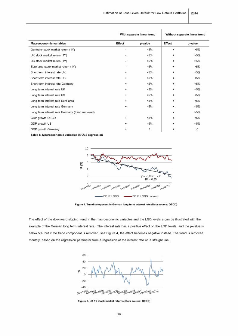
Macroeconomic variables Effect p-value Effect p-value Germany stock market return (1Y) - >5% + >5% UK stock market return (1Y) - <5% + >5% US stock market return (1Y) - >5% + >5% Euro area stock market return (1Y) - >5% + >5% Short term interest rate UK + <5% + <5% Short term interest rate US + >5% + <5% Short term interest rate Germany + <5% + <5% Long term interest rate UK + <5% + <5% Long term interest rate US + >5% + <5% Long term interest rate Euro area + >5% + <5% Long term interest rate Germany + <5% + <5% Long term interest rate Germany (trend removed) - >5% GDP growth OECD + >5% + <5% GDP growth US + >5% + <5% GDP growth Germany + 1 + 0 Table 6. Macroeconomic variables in OLS regression

The effect of the downward sloping trend in the macroeconomic variables and the LGD levels a can be illustrated with the

example of the German long term interest rate. The interest rate has a positive effect on the LGD levels, and the p-value is

below 5%, but if the trend component is removed, see Figure 4, the effect becomes negative instead. The trend is removed

monthly, based on the regression parameter from a regression of the interest rate on a straight line.

Figure 4. Trend component in German long term interest rate (Data source: OECD)

y = -0,02x + 7,2 R² = 0,85

0

2

4

6

8

10

IR (%

)

DE IR LONG DE IR LONG no trend

-40

-20

0

20

40

60

%

Figure 5. UK 1Y stock market returns (Data source: OECD)


27

Instead of removing the trend from the macroeconomic time series one could incorporate a separate linear trend in the

regression in order to capture the decreasing trend in the LGD levels. Such a trend has a significant negative effect on the

estimated LGD levels in an OLS regression. If such a trend is incorporated the stock market return parameters change sign

and have a negative effect on the LGD levels. The other variables still have a positive effect but the p-values increase and

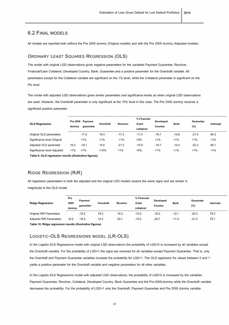
many are now not significant, see Table 6. The most significant stock market return parameter is the UK stock market return.

This time series, showed in Figure 5, bears more characteristics of a business cycle proxy than for example the long term

interest rates in Figure 4. The stock market returns and the interest rates have the advantage of being publically available at

every point in time unlike GDP growth which is only known subsequently. It could also be argued that both stock market return

and interest rate figures are forward looking to some extent which would be a benefit since it is the macroeconomic

environment during the bankruptcy process and not at the default date that is believed to influence the LGD levels.

However, in a practical model, a macroeconomic variable sometimes results in unintuitive splits in the tree models with higher

LGDs during supposed better economic times. Secondly, tree models sometimes create leaves based on very small differences

in the macroeconomic variables which seem unlikely to hold out of sample. Furthermore, as previously mentioned the LGD

used in the report of credit risk must be a so called “ ownturn G ”, i.e. reflecting the G in a downturn environment.

Because of this the effect of the macroeconomic variable needs to be both large enough in magnitude to create a substantial

difference during economic downturns and affect observations of all kinds. The macroeconomic variable introduced here fails to

have a substantial effect in an OLS model and does only affect parts of the tree models since the splits are too far down in the

trees. Due to these reasons no macroeconomic variable was used in the final models.

SENIORITY & FACILITY TYPE Several studies have found the seniority of the claim to be one of the most important determinants of LGD. However, the

seniority parameter failed to prove significant in an OLS regression and actually indicated a positive relationship between LGD

and seniority. It was therefore dropped from the models.

Most academic LGD studies focus on loans and bonds but since also other facility types differ in usage and risk profile, the

facility type can be used as a risk driver. In this sample, the dummy variables for the facility types payment guarantee, overdraft,

and revolver has been found to significantly affect the LGD levels in an OLS regression. However, the dummy variables for the

types bond, loan and derivatives and securities claim failed to prove significant in the sample. In the F-tree model the loan

dummy is once again included since it has been proved significant in subsets of the data.

COLLATERAL According to the academic literature collateral should be an important determiner of the realized LGD. While this effect was

found in the sample the effect was not as significant as for other variables and was sensitive to specifications of the variable. It

is not only the size of the collateral which matters for the realized recovery. While financial collateral usually can be converted

to cash easily, physical collateral can be cumbersome to sell, especially to a fair value, since the number of buyers can be few

and the market illiquid. To mitigate this problem the variable used in the models is the percentage of financial and cash

collateral out of the defaulted amount. Other types of collaterals are not used in the models. The variable is also capped at

100 %, meaning that any collateral worth more than 100 % of the defaulted amount will still only count as 100%.


28

GEOGRAPHIC REGION (DEVELOPED COUNTRY) A model utilizing exposures from all over the world needs to check for systematic differences between geographic regions.

Several ways of grouping countries were tested (including EU, EEA, Euro zone, North America, Scandinavia, OECD, Emerging

markets etc.). The distinction between developed and developing countries was chosen for several reasons. First, it yields two

substantial groups in the sample. Secondly, it is intuitive and there is no need to make judgemental decisions regarding for

instance whether Denmark should be grouped with the Euro countries or not. It also gave reasonable and significant results in

an OLS regression and no residual group with countries not belonging to any group appeared. The variable in the models is a

dummy variable indicating whether the borrower’s country of jurisdiction is a developed country or not. If the country of

jurisdiction is unknown the country of residence is used instead.

INDUSTRY (BANKS) Since this study considers only the financial industry grouping of observations on industry level is not possible. However some

differences regarding the type of borrower can be seen in the data. Since banks face higher regulatory requirements than other

financial institutions it could be supposed that this would influence the realized LGD levels. Another explanation could be that

banks are more likely to be saved when facing default due to their importance to the economy. The data gives some support to

this theory when looking at the proportion of nominal LGDs equalling zero. The variable used in the models is a dummy

variable indicating whether the counterparty is a bank or not.

Banks Non-bank Financial institutions Nominal LGDs =0 60% 42% Table 7. Bank and non-banks with nominal LGD equal to zero (illustrative figures)

SIZE OF FIRM & EXPOSURE Many academic studies use the size of the exposure as an explanatory variable for LGD levels (Bastos, 2010; Khieu et al.,

2012). While this could help explaining LGD for e.g. SMEs, where a company has just one or a few lenders, it is probably not

useful for the case of a low default portfolio with a lot of banks and institutions since these entities typically have many liabilities

to a huge amount of counterparties. The argument that higher default amounts lead to lower recovery rates as banks are

unwilling to push larger loans to default resulting in lower recoveries when loans actually default which has sometimes been

proposed (Khieu et al. 2012) seems unlikely to be valid for the kind of obligors in this data. Since banks and other financial

institutions have a huge amount of creditors and exposures it is usually not up to one single creditor whether to push the

institution to default. Furthermore, including the size of the exposure is also problematic from a practical point of view. It is hard

to justify for business units why two small loans should have a larger (or smaller) expected loss than one big.

The size of the firm has not been tested as an explanatory variable for realized LGD levels since it is in most cases not

reported to the database in order to ensure the anonymity of the data.

INDUSTRY DISTRESS Industry distress as a risk driver is not considered since only the financial industry is included in this study and it is believed

that the state of the economy can serve as a reasonable proxy for the state of the financial industry. The use of

macroeconomic variables as a proxy for the degree of distress in the financial industry can be motivated by the fact that


29

financial crises often lead to severe recessions (Reinhart and Rogoff, 2009). The findings by Cebula et al (2011) indicating a

positive relationship between the growth rate of real GDP and the failure rate of banks further supports the use of this proxy. It

also seems intuitive from a theoretical viewpoint since a stronger economy should result in a stronger performance of bank

loans, reducing the risk of bank failures.

LEVERAGE Similar to firm size, the borrower’s leverage is not included in the database.

GUARANTEE A guarantee from a third party is expected to decrease the LGD levels. This effect has been proved significant in an OLS

regression. The variable in the models is the percentage of the defaulted amount which is guaranteed. The variable is capped

at 100% meaning that observations with a higher percentage guaranteed still receive the value 100%.

UTILISATION RATE A variable capturing the utilization rate at the event of default failed to prove significant in an OLS regression. Since it is also

likely that the utilisation rate soars just before the event of default it is not appropriate to use as a risk driver from a practical

viewpoint. Utilisation rate was therefore dropped from the models.


30

DEFAULT YEAR (PRE-2005 DUMMY) Incorporating a yearly trend in the data can be problematic from a practical point of view since the model would then suggest

that the LGD levels are decreasing in time. If the model is to be used in practice all predictions of future LGDs would be

adjusted downwards with some constant times the number of years in the sample, 20 years in this case. This is problematic for

two reasons. First, in this study the adjustment is rather large in magnitude and may thereby be hard to justify. Secondly the

model would run into problems if the LGD levels start to

increase again and the linear effect disappears. Instead of

using a linear trend throughout the sample period a dummy

variable for early observations can be included. This

approach has several advantages. Firstly it is easier to

justify since the effect is restricted to early observations and

not the whole sample. Secondly the effect will fade away

when more observations are included and no problems will

arise if the linear downward sloping trend in the data

disappears with new observations. Thirdly, a pre-2005

dummy can be justified from a theoretical viewpoint since

this was the year when the Basel default definitions were

released. One could suspect that before these definitions

were effective, the default definitions were stricter and too

few observations with a zero loss were reported as defaults.

This is however not supported by the data in this study. The

number of observations where the nominal LGD equals zero

does not seem to increase over time, see Figure 6. However, the choice of 2005 for the dummy variable still seems reasonable

when looking at the data. Table 8 shows p-values from the OLS model for different choices of year. The year 2005 gives a very

low p-value for the dummy variable and there are still a substantial number of observations after this year.

While it seems reasonable from a mathematical point of view to try to include all observations and capture differences in

reporting habits it can be problematic to justify that the average LGD level in the sample is too high and should be adjusted

downwards. The test results are therefore reported both with and without such an adjustment.

Year p-value year dummy # obs. later than

1991 >10% 676 1992 >10% 674 1993 <1% 670 1995 <1% 660 1996 <1% 657 1997 <1% 655 1998 <1% 652 1999 <10% 530 2000 <10% 504 2001 <10% 485 2002 <1% 460 2003 <1% 420 2004 <1% 392 2005 <1% 365 2006 <1% 340 2007 <1% 310 2008 <1% 276 2009 >10% 156 Table 8. Splitting year into dummy variable (illustrative figure)

1 2 3 4 5

Figure 6. Proportion of nominal LGD equal to zero


31

6.2 FINAL MODELS All models are reported both without the Pre 2005 dummy (Original models) and with the Pre 2005 dummy (Adjusted models).

ORDINARY LEAST SQUARES REGRESSION (OLS) The model with original LGD observations gives negative parameters for the variables Payment Guarantee, Revolver,

Financial/Cash Collateral, Developed Country, Bank, Guarantee and a positive parameter for the Overdraft variable. All

parameters except for the Collateral variable are significant on the 1% level, while the Collateral parameter is significant on the

5% level.

The model with adjusted LGD observations gives similar parameters and significance levels as when original LGD observations

are used. However, the Overdraft parameter is only significant at the 10% level in this case. The Pre 2005 dummy receives a

significant positive parameter.

OLS Regression Pre 2005 dummy

Payment guarantee

Overdraft Revolver % Financial /Cash collateral

Developed Country

Bank Guarantee (%)

Intercept

Original OLS parameters -17.2 19.3 -17.3 -11.0 -19.1 -14.8 -21.4 84.3 Significance level Original <1% <1% <1% <5% <1% <1% <1% <1% Adjusted OLS parameter 16.3 -19.1 14.6 -21.2 -10.8 -19.7 -14.2 -22.3 80.1 Significance level Adjusted <1% <1% <10% <1% <5% <1% <1% <1% <1% Table 9. OLS regression results (illustrative figures)

RIDGE REGRESSION (RIR) All regression parameters in both the adjusted and the original LGD models receive the same signs and are similar in

magnitude to the OLS model.

Ridge Regression Pre 2005 dummy

Payment guarantee


Developed Country

Bank Guarantee (%)

Intercept

Original RiR Parameters -16.2 19.3 -16.3 -10.2 -18.2 -12.1 -20.3 79.3 Adjusted RiR Parameters 16.2 -18.2 14.2 -20.1 -19.2 -20.7 -11.2 -21.3 78.1 Table 10. Ridge regression results (illustrative figures)

LOGISTIC-OLS REGRESSIONS MODEL (LR-OLS) In the Logistic-OLS Regressions model with original LGD observations the probability of LGD=0 is increased by all variables except

the Overdraft variable. For the probability of LGD=1 the signs are reversed for all variables except Payment Guarantee. That is, only

the Overdraft and Payment Guarantee variables increase the probability for LGD=1. The OLS regression for values between 0 and 1

yields a positive parameter for the Overdraft variable and negative parameters for all other variables.

In the Logistic-OLS Regressions model with adjusted LGD observations, the probability of LGD=0 is increased by the variables

Payment Guarantee, Revolver, Collateral, Developed Country, Bank Guarantee and the Pre-2005-dummy while the Overdraft variable

decreases the probability. For the probability of LGD=1 only the Overdraft, Payment Guarantee and Pre 2005 dummy variable


32

increase the probability. The Pre 2005 dummy was expected to receive a negative parameter in the regression for P(LGD=0) as more

observations of no loss is expected to be included in the data set after 2005. This might be an indication that the theoretical reason

for including the Pre 2005 dummy is not supported by the data. The OLS regression shows a positive parameter only for the Pre

2005 dummy variable, all other parameters have negative signs.

Logistic-OLS Regressions model

Pre 2005 dummy

Payment guarantee


Developed Country

Bank Guarantee (%)

Intercept

Original 0 < LGD <1 -8.3 8.5 -9.2 -10.2 -4.6 -9.2 -15.5 61.5 Original P(LGD=0) 3.5 -0.8 2.4 0.5 3.1 2.2 2.6 -7.4 Original P(LGD=1) 0.1 1.4 -0.7 -0.7 -1.1 -0.8 -2.3 -0.1 Adjusted 0 < LGD <1 5.3 -7.3 -0.3 -10.3 -11.1 -2.7 -7.0 -15.1 57.2 Adjusted P(LGD=0) 1.7 4.0 -2.3 2.3 0.5 2.8 1.6 2.5 -8.3 Adjusted P(LGD=1) 2.3 0.7 0.5 -1.0 -1.5 -1.3 -0.7 -2.3 -1.5 Table 11. Logistic-OLS Regressions results (illustrative figures)

TRIMMED LOGISTIC-OLS REGRESSIONS (TLR-OLS) In the Trimmed Logistic-OLS Regressions model the probability of LGD=0 is equal to the probability of LGD=0 in the LR-OLS

model above, that is the regressions are identical. The OLS regression for the original observations gives a positive parameter

for the Overdraft variable and negative parameters for the other variables, just like in the LR-OLS model. In the adjusted model

the Pre 2005 dummy has a positive parameter in the OLS regression. All other effects are in line with the original model but the

positive effect of Overdraft is much lower in the adjusted LGD model. The parameters for all variables apart from the Overdraft

variable receive the same signs in the TLR-OLS model as in the LR-OLS model but most differ in magnitude.

Trimmed Logistic-OLS Regressions model

Pre 2005 dummy

Payment guarantee


Developed Country

Bank Guarantee (%)

Intercept

Original 0 < LGD -5.5 20.7 -13.8 -14.0 -12.9 -13.6 -25.2 79.1 Original P (LGD=0) 3.5 -0.8 2.4 0.5 3.1 2.2 2.6 -7.4 Adjusted 0 < LGD 18.3 -1.2 7.2 -15.2 -15.3 -10.2 -10.8 -26.3 64.4 Adjusted P (LGD=0) 1.7 4.0 -2.3 2.3 0.5 2.8 1.6 2.5 -8.3 Table 12. Trimmed Logistic-OLS Regressions results (illustrative figures)

REGRESSION TREE (RT) The regression tree generated with original LGD observations, Figure 7, starts with splits on the product types Overdraft and

Revolver. If the observation is a revolver the sample is then split upon Developed/Developing Country. If the observation is

neither an overdraft nor a revolver the sample is split upon the level of guarantee. The observations with low guarantee levels

are then split in Payment Guarantees and Non Payment Guarantees.

The regression tree with adjusted LGD observations, Figure 8, starts with the same 4 splits. The observations in the group with

low guarantees are however split in Developed and Developing Countries before splitting on Payment Guarantees.


33

F-TREE (FT) The F-tree in Figure 9 is based on the original LGD values, that is, early observations have not been adjusted. The data is split

into 9 different leaves. The F-tree in Figure 10 has been created based on adjusted LGD values prior to 2005. Here the data is

split into 10 different leaves. Both models include the Loan product type which failed to prove significant in the regression

models. In general the two models are similar apart from an extra split on the guarantee level in the adjusted LGD model.

Both the F-tree and the Regression tree could easily be modified due to qualitative considerations without a large worsening in

the test results. It could also be noted that the F-tree model produces larger trees than the RT model where the minimum leaf

size is set to 7.5% of the sample.

Figure 7. Regression tree based on original LGD observations (illustrative figures)

Financial institutions (676)

1 Overdraft (64)

55% Non overdraft

Revolver

2. Developed Country (62)

20%

3. Developing Country (59)

35%

Non Revolver

Guarantee <48,25%

4. Payment Guarantee (200)

20%

5. Non Payment Guarantee (230)

45%

6. Guarantee >48,25% (61)

17%

Figure 8. Regression tree based on adjusted LGD observations (illustrative figures)

Financial institutions

(676)

1 Overdraft (64)

48% Non overdraft

Revolver

2. Developed Country (62)

17%

3. Developing Country (59)

30%

Non Revolver

Guarantee <48,25%

5. Developing country (80)

52%

Developed Country

6. Payment Guarnatee(160)

9%

7. Non Payment Guarantee(190)

39%

8. Guarantee >48,25% (61)

13%

Figure 10. F-tree based on adjusted LGD observations (illustrative figures)


(676)

Non Payment guarantee

Revolver

Developing country

4 Guar. <70% (25) 13%

5 Guar. >70% (46) 36%

3 Developed country (53)

12%

Non Revolver

Guar. <70%

Bank

Loan

9 Developing country (40)

47%


33%

8 Non loan (109) 49%

7 Non Bank (29) 66%

6 Guar. >70% (30) 15%

Payment guarantee


43%


8%

Figure 9. F-tree based on original LGD observations (illustrative figures)


(676)

Non Payment guarantee

Guar. < 70%

Non Revolver

Bank

Loan


37%


54%

7 No loan (109) 53%

6 Non Bank (29) 68%

Revolver


17%

5 Developing Country (45)

44%

3 Guar.>70% (59) 18%

Payment guarantee


48%


9%


34

6.3 TEST RESULTS

The models have been evaluated based on the statistical techniques outlined in Section 5.

PREDICTIVE POWER The results of the within sample, out of sample and out of time tests are presented in Table 13 and 14. Within sample the LR-

OLS, TLR-OLS, FT and RT models give unbiased estimates while the RiR and OLS models have small positive biases due to

the truncation of estimates to the [0,1] interval. This is true for the estimations based both on original and adjusted LGD

observations for all models except LR-OLS which produces a small negative bias using adjusted LGD levels. In terms of MAE

and R2 the FT model produces the best results within sample. However the differences between the models are not large. All

models produce positive R2 values and substantially lower MAE than using historical average in the within sample test.

The errors increase out of sample but not to a large extent. In the out of sample test the FT model gives the lowest MAE

regardless of whether observations are adjusted or not. In terms of ME all models seem to be close to unbiased. The original

observations result in similar R2 values for all models except for RT which has a substantially lower R2 value. Using adjusted

observations the LR-OLS and TLR-OLS models give higher R2 values than the other models. All models give lower errors and

higher R2 values than using the Historical average approach out of sample.

The F-tree model gives the largest errors out of time, even larger than the historical average approach, both when observations

are adjusted and not. The lowest errors are produced by the LR-OLS and TLR-OLS models when observations prior to 2005

are adjusted. The LR-OLS model is the only model to produce positive R2 values with original observations. In general no

model produces substantially better results than using the Historical average approach in the out of time test. Once again, the

limitations of the out of time test described in Section 5 needs to be taken into account.

Overall, errors are lower when observations prior to 2005 are adjusted.

Within sample Out of sample Out of time ME MAE R2 ME MAE R2 ME MAE R2 OLS 0.5 22.1 0.34 0.3 (4.3) 22.8 (1.6) 0.31 (0.14) 8.2 (11.8) 26.1 (2.8) -0.16 (0.32) RiR 0.3 22.1 0.34 0.2 (5.1) 22.8 (1.5) 0.31 (0.09) 7.8 (11.0) 26.1 (3.3) -0.14 (0.30) LR-OLS 0.0 21.4 0.36 0.1 (3.8) 21.9 (2.0) 0.32 (0.07) 8.3 (9.5) 26.0 (2.8) 0.13 (0.16) TLR-OLS 0.0 21.,3 0.36 0.0 (2.8) 21.7 (2.6) 0.32 (0.07) 7.8 (9.0) 26.0 (3.0) -0.17 (0.32) RT 0.0 24.7 0.23 0.2 (2.7) 24.8 (1.5) 0.24 (0.11) 2.8 (3.2) 25.4 (3.7) -0.11 (0.29) FT 0.0 20.9 0.36 -0.1 (3.2) 21.4 (2.0) 0.32 (0.09) 17.0 (11.5) 30.9 (0.2) -0.61 (0.73) Hist 0.0 28.9 0.00 -0.2 (4.7) 29.0 (1.3) -0.02 (0.04) 1.9 (5.3) 27.4 (6.0) -0.05 (0.08) Standard deviations in brackets Table 13. Predictive power for original LGD levels (illustrative figures)


35

The estimated LGD levels depend of course on the model chosen. Table 16 summarizes LGD estimates for the example

portfolio defined in Section 5 as well as for three specific exposures. The exposures are described in Table 17. The choice of

model clearly influences the estimated LGD levels, especially for specific exposures. On a portfolio with different exposures the

effects net out to some degree and the overall LGD estimate does not differ as much between different models. Since the tree

models group exposures and assign the same LGD to the whole group the reasonability of the grouping needs to be justified

from a theoretical viewpoint. The effect of the grouping on a real portfolio needs to be considered since many exposures might

end up in the same leaf. This is especially important since the LGD estimates differ a lot in magnitude as seen in Table 16.

Furthermore, tree models might fail to distinguish between exposures of rather different nature which could be problematic in

practice.

Description Exposure 1 Unsecured bond exposure towards bank in developed country Exposure 2 Collaterized loan to non-bank financial institution in developing country Exposure 3 Revolver to non-bank financial institution in developed country Table 17. Description of exposures in Table 16

Within sample Out of sample Out of time ME MAE R2 ME MAE R2 ME MAE R2 OLS 0.3 21.9 0.36 0.3 (2.8) 22.4 (1.6) 0.32 (0.12) 3.2 (11.5) 24.1 (3.8) 0.05 (0.17) RiR 0.1 22.0 0.35 1.1 (2.3) 22.4 (1.6) 0.31 (0.11) 2.5 (11.2) 23.8 (4.0) 0.06 (0.15) LR-OLS -0.2 20.8 0.40 0.3 (3.9) 21.5 (2.0) 0.36 (0.07) -0.4 (6.1) 23.7 (4.4) 0.13 (0.07) TLR-OLS 0.0 21.0 0.39 0.0 (2.9) 21.5 (1.0) 0.35 (0.07) -0.1 (15.1) 23.6 (3.8) 0.05 (0.06) RT 0.0 20.5 0.31 0.1 (2.5) 20.5 (1.5) 0.32 (0.10) 3.5 (5.7) 23.6 (3.3) 0.10 (0.11) FT 0.0 19.4 0.35 -0.2 (1.5) 19.9 (0.6) 0.31 (0.12) 11.8 (8.3) 28.7 (0.9) -0.20 (0.47) Hist 0.0 26.6 0.0 0.2 (4.0) 26.6 (1.2) -0.02 (0.06) -1.1 (7.5) 25.8 (6.2) 0.01 (0.04) Standard deviations in brackets Table 14. Predictive power for adjusted LGD levels (illustrative figures)

Example Portfolio Exposure 1 Exposure 2 Exposure 3 OLS 36.6 39.4 67.3 36.9 RiR 35.7 39.2 64.7 35.4 LR-OLS 31.6 39.4 55.9 36.9 TLR-OLS 33.4 41.1 61.1 38.8 RT 35.4 45.7 45.7 18.3 FT 33.8 54.9 70.5 17.0 Hist 32.9 32.9 32.9 32.9 Table 16. LGD estimates (illustrative figures)


36

LGD DISTRIBUTIONS FOR EXAMPLE PORTFOLIO Bootstrapping the original data and recalculating the results for the example portfolio defined in Section 5 yields the distributions of LGD estimates presented in Table 18 and the percentiles presented in Table 19. The models using linear regressions generally results in a larger dispersion than the tree models.

OLS RiR LR-OLS TLR-OLS RT FT

Table 18. LGD distribution for example portfolio (illustrative graphs)

OLS RiR LR-OLS TLR-OLS RT FT 1st Percentile 29.3 28.6 24.4 26.8 28.1 29.0 Mean 36.8 35.9 31.4 35.6 31.8 33.8 99th Percentile 45.0 43.8 39.9 46.1 36.3 39.1 Table 19. LGD percentiles for example portfolio (illustrative figures)

CORRELATION MATRIX OF LGD ESTIMATES A correlation matrix of the LGD estimates produced by the example portfolio is presented in Table 20. As expected there is a

strong positive correlation between the models. The correlation is however stronger between the models based on linear

regression. The correlation between the two tree models is the lowest of all correlations in the matrix, while all correlations

between based on linear regression are close to 1.

USING MODELS IN PRACTICE

A major difference between the tree models, RT and FT models, and the models based on linear regressions (OLS, RiR, LR-

OLS and TLR-OLS) is that linear regressions give rise to an infinite set of possible LGD estimates. As a portfolio might consist

of exposures with characteristics not found in the sample it is difficult to get an overview of the possible outcomes of LGD

estimates. In the tree models all possible outcomes of LGD estimates are stated beforehand. However, consistency in ranking

is not assured in the tree models. It is possible that “better” exposures receive a higher G estimate since they happen to be

grouped with “worse” exposures having high G s. In the models including linear regressions (OLS, RiR, LR-OLS and TLR-

OLS) consistency in ranking is assured since all observations get the same reduction or penalty for a certain characteristic.

OLS RiR LR-OLS TLR-OLS RT FT OLS 1.00 1.00 0.95 0.96 0.60 0.64 RiR 1.00 0.95 0.96 0.62 0.65 LR-OLS 1.00 0.99 0.56 0.71 TLR-OLS 1.00 0.60 0.71 RT 1.00 0.51 FT 1.00 Table 20. Correlation matrix of LGD estimates in example portfolio (illustrative figures)


37

The LGD estimates generated by OLS and RiR might also be higher than 1 or lower than 0 for certain input parameters. Since

these estimates need to be truncated to the [0,1] interval a small bias may occur as seen in the MEs. In the tree models the

only possible outcomes of LGD estimates are stated in the leaves. As each estimate constitutes of an average of actual LGD

observations the estimates are bounded between 0 and 1. Both the LR-OLS and TLR-OLS models can potentially produce

estimates smaller than 0 or larger than 1 but this is not as likely as for the OLS and RiR models since the OLS estimate only

accounts for a part of the estimated value. However, in an LDP setting where only a small amount of default data is available

the LR-OLS and TLR-OLS models produce rather uncertain estimates since the already small sample is divided into smaller

subsets and information is removed when the regression samples are created. In this setting an OLS or RiR model gives

steadier estimates of LGD as the regression uses the full sample. It might also be hard to evaluate the reasonability of the

logistic regression parameters since theory might indicate whether a certain variable should influence the average LGD level

positively or negatively but not whether the specific case of full or no recovery is more or less likely. This problem is potentially

even more severe in a LDP setting since the need for a qualitative check of the reasonability of the parameters is more

important due to the uncertainty resulting from the small sample.

LGD Collateral value / Defaulted amount (%)

100 0.0 0 1.43 10 1.43 0 2.310 10 2.311 80 2.312 50 2.313 5 2.313 0 2.620 0 2.622 30 2.67 0 2.68 0 3.01 0 48 10 72 Table 15. Splitting continuous variables (illustrative figures)

The LDP setting also affects the RT model as the minimum leaf size has to be a rather large percentage of the total sample in

order to include enough observations for a relatively stable estimate. In the FT model the algorithm itself handles this problem

to some extent. If the difference between two groups is statistically significant then a split of the groups is performed. In this

way the model finds an optimal level of splits for a given sample size. However, too small leaves could still be problematic from

a practical point of view since the average LGD could change substantially if an outlier is added. In practice one would not like

the estimates to change too much when new observations are incorporated.

Given that the set of explanatory variables primarily consists of dummy variables the advantage of the RT model being able to

split continuous variables at the optimal place is not used to a large extent in this context. The two continuous variables used in

this study, guarantee and collateral size, also both have a bimodal distribution with many observations close to 0 and 1. This

might result in unintuitive and inexact splitting points as can be seen in Table 15. Even if a certain level of collateral is optimal


38

to split upon from a reduction of standard deviation perspective it might not seem appropriate from a qualitative perspective.

This problem is likely to be more severe in a LDP setting, given the small sample size. An alternative approach is to use a

qualitative opinion to create one or more dummy variables replacing the continuous variable. The potential splitting points could

then be chosen based on an expert opinion and the RT algorithm decides which ones to use.

Both tree models also give the opportunity to include expert opinions in the construction of the models. It is possible to make

small deviations from the algorithms of constructing the tree and instead of using the optimal split using another split if this

seems more appropriate from a qualitative perspective. In this sense the tree models could be preferred above the other

models when it comes to implementing a model in practice. One should bear in mind however, that also the other models can

use expert opinions when deciding e.g. which variables to include in the models and where to cap them.

When assessing the LGD levels one needs to remember the LDP setting and the small amount of data available. The Basel accord states that “the less information a bank has, the more conservative must be its assignments of exposures to borrower and facility grades or pools” (BIS, 2006, § 411).

6.4 SUMMARY OF RESULTS

Some of the risk drivers believed to be suitable to include in the models have been deemed inappropriate to include for

practical or mathematical reasons. The macroeconomic variables have been left out due to the difficulties of finding a variable

giving the expected negative influence on the LGD estimate as well as practical concerns regarding the possibilities to produce

downturn estimates by using such a variable. The seniority of the defaulted facility has, in contrast to most academic studies,

been left out since it failed to prove significant in an OLS regression. This could be the result either of the small sample

available or alternatively a characteristic of exposures towards financial institutions. Many academic studies use the size of the

exposure as a risk driver for LGD. The exposure size has been deemed inappropriate to include partly due to the small size of

the exposure in relation to the total liabilities of a global financial institution and partly due to the practical difficulties in

explaining to a business unit why two small loans should differ from one large in LGD. Furthermore the utilisation rate has been

considered inappropriate since it is likely to soar just before the default event and hence cannot be used to predict future LGD

levels. Industry distress has not been considered since it is believed to be heavily linked to the macroeconomic environment.

From a mathematical viewpoint adjusting the observed values prior to 2005, the year when the Basel default definitions were

publicized, would make the models produce better estimates. This adjustment could however be problematic to justify and

might therefore not be suitable for a practical model. All tested models produce better results than using the historical average in within and out of sample testing, both with and

without adjustment of observations prior to 2005. The FT model produces the best results within sample and out of sample if

the original LGD observations are used. No model produces good results in the out of time testing but the FT model is the

worst and is actually worse than using the Historical average approach. On the other hand, the tree models have some

advantages from a practical viewpoint. The estimates are guaranteed to lie within the [0,1] interval since the estimates are

averages of actual observations and it is easy to include an expert opinion when creating the models. Furthermore, the

bootstrapping exercise indicates that the tree models give more stable LGD estimates for the example portfolio defined in

Section 5. The TLR-OLS and particularly the LR-OLS model might be less suitable in a LDP setting since information is

removed and the already small sample is divided into smaller subsets and separate regressions are performed on these


39

subsets. This might result in more unstable estimates. Since the LR-OLS does not produce better results than the TLR-OLS

model, the TLR-OLS model might be more suitable in a LDP setting as it only divides the sample once. On a portfolio level the

tested models give similar LGD estimates. However the estimates may differ substantially for specific exposures.


40

7 CONCLUDING REMARKS LGD estimates should “reflect the experience and practice of the individual institution as well as the external environment in

which it operates” (BIS, 2006, § 70). This implies that a financial institution cannot simply rely on general industry estimates for

the parameters but need to adjust them in order to account for institution specific factors. While this is done to some extent by

adjusting the LGD estimates based on the proportion of different facility types and collateral etc. the institution in question

would also need to justify that the risk they are facing can be assessed by using pooled industry data, or alternatively make

some adjustment.

The sample used in this study consists of pooled industry data. This means that the same default can be reported several

times by different banks and the actual number of default events might be much smaller than the number of observations.

Unfortunately it is hard to tell which observations belong to the same default event since the data is anonymous. Even though

observations of the same default are not copies of each other they could potentially be similar which reduces the usefulness of

the data set. This reduces the applicability of the out of sample testing since not all observations are independent.

Covered bonds and repos are two types of exposures common in LDPs where the lack of data is particularly severe. For these

kind of exposures, a judgemental model based on expert opinions probably needs to be applied if they are to qualify for IRB

treatment. This is in line with the recommendations by the British Bankers Association, the London Investment Banking

Association and ISDA that no portfolios should be ruled out from IRB treatment but that it cannot be taken as a premise that all

types of exposures will meet the requirements and that business experience can be used to create judgemental models if the

data available is insufficient (ISDA, 2005).


41

8 REFERENCES Acharya, V; Bharath, S; Srinivasan, A (2007), ‘ oes Industry-Wide Distress Affect Defaulted Firms? Evidence from Creditor

Recoveries’, Journal of Financial Economics, 85 pp. 787–821.

Altman, E; Resti, A; Sironi, A (2004). ‘ efault Recovery Rates in Credit Risk Modelling: A Review of the iterature and

Empirical Evidence’, Economic Notes, 33 (2) pp. 183-208.

Andritzky, J (2005), ‘ efault and Recovery Rates of Sovereign Bonds: A Case Study of the Argentine Crisis‘, Journal of Fixed

Income, 15 (2) pp. 97-107

Andritzky, J; Singh, M (2006),’The Pricing of Credit efault Swaps uring istress’, IMF Working Paper, WP/06/254

Araten, M; Jacobs, M Jr; Varshney, P (2004), ‘Measuring G on Commercial oans: An 18-Year Internal Study’, The RMA

Journal, May 2004

Bank for International Settlements (BIS) (2005a), ‘Guidance on Paragraph 468 of the Framework ocument’, (July 2005)

Bank for International Settlements (BIS) (2005b), ‘Validation of low-default portfolios in the Basel II Framework’, Newsletter No.

6 (September 2005)

Bank for International Settlements (BIS) (2006), ‘International Convergence of Capital Measurement and Capital Standards - A

Revised Framework Comprehensive Version’, June 2006

Bastos, J (2010), ‘Forecasting bank loans loss-given-default’, Journal of Banking & Finance, 34 (10) pp. 2510-2517

Bellotti, T; Cook, J (2008), ‘Modelling and estimating Loss Given Default for credit cards’, CRC Working paper 08-1

Berd, A (2005), ‘Recovery Swaps’, Journal of Credit Risk, 1 (3), pp. 61-70

Black, P "greedy algorithm", in Dictionary of Algorithms and Data Structures [online], Vreda Pieterse and Paul E. Black, eds. 2

February 2005. (accessed 2014-03-18) Available from: http://www.nist.gov/dads/HTML/greedyalgo.html

Brady, B; Chang, P; Miu, P; Ozdemir, B; Schwartz, (2006), ‘ iscount Rate for Workout Recoveries: An Empirical Study’,

Working Paper, (accessed 2014-03-25) Available from: http://www.fdic.gov/bank/analytical/cfr/2006/sept/MiuP.pdf

Calabrese, R (2012), ‘Estimating bank loans loss given default by generalized additive Models’, UCD Geary Institute Discussion

Paper Series, WP2012/24

Cebula, R; Koch, J; Fenili, R (2011), ‘The Bank Failure Rate, Economic Conditions and Banking Statutes in the U.S., 1970–

2009’, Atlantic Economic Journal, 39 (1), pp.39-46

Committee of European Banking Supervisors (CEBS) (2006), ‘Guidelines on the implementation, validation and assessment of

Advanced Measurement (AMA) and Internal Ratings Based (IRB) Approaches’ (accessed 2014-03-18) Available from:

https://www.eba.europa.eu/documents/10180/15917/GL10.pdf/de6ea199-6f33-4228-9665-63e08dde767d


42

Christensen, J (2005), ‘Joint Estimation of Default and Recovery Risk: A Simulation Study‘, Working Paper, (accessed 2014-03-

18) Available from: http://www.fdic.gov/bank/analytical/cfr/2006/apr/Christensen_Paper.pdf

as, S and Hanouna, P (2008), ‘Implied Recovery’, FDIC Center for Financial Research Working Paper, 2009-05

ermine, J and Carvalho, C (2005), ‘Bank loan losses-given-default: A case study’, Journal of Banking & Finance, 30 pp. 1219-

1243

Frye, J (2000), ‘ epressing Recoveries’, Risk, 13(11) pp. 108–111.

Gupton, G (2005), ‘Advancing oss Given efault Prediction Models: How the Quiet Have Quickened’, Economic Notes by

Banca Monte dei Paschi di Siena SpA, (34-2) pp. 185–230

Gürtler, M and Hibbeln, M (2013), ‘Improvements in loss given default forecasts for bank loans’, Journal of Banking & Finance,

37 pp. 2354-2366

Hayden, E (2003), ‘Are Credit Scoring Models Sensitive With Respect to Default Definitions? Evidence from the Austrian

Market’. Working paper, February 2003

IS A, IBA, BBA (2005), ‘ ow efault Portfolios - Joint Industry Working Group iscussion Paper’, January 2005, (accessed

2014-03-18). Available from: http://www.isda.org/c_and_a/pdf/ISDA-LIBA-BBALowDefaulPortfolioPaper-January2005.pdf

Khieu, H; Mullineaux, ; Yi, H (2012), ‘The determinants of bank loan recovery rates‘, Journal of Banking & Finance, 36 pp.

923-933

Kofman, J (2011) ‘Overcoming challenges in P / G modelling in the absence of high quality and rich data’, Moody’s Analytics

ang, H (2012), ‘Topics on Applied Mathematical Statistics’, July 2012, version 0.93

Loterman, G; Brown, I; Martens, D; Mues, C; Baesens, B (2012), ‘Benchmarking regression algorithms for loss given default

modeling‘, International Journal of Forecasting, 28(2012) pp. 161-170

Moody’s Analytics New York (2005), ‘ efault and Recovery Rates of Corporate Bond Issuers, 1920-2004’, New York

PECDC (2013a), ‘PEC C ownturn G Study’, 17 ecember 2013 (accessed 2014-03-18). Available from:

http://www.pecdc.org/uploads/PECDC%20Default%20Rate%20Study%202013.pdf

PECDC (2013b), ‘What is PEC C?’, Online, (accessed 2014-04-02), Available from: http://www.pecdc.org

Pluto, K; Tasche, (2005), ‘Estimating Probabilities of efault for ow efault Portfolios’, Working Paper, (accessed 2014-03-

18) Available from: http://ssrn.com/abstract=635301

Qi, M and Zhao, X (2011), ‘Comparison of modeling methods for Loss Given Default’, Journal of Banking & Finance, 35 (2011)

pp. 2842-2855

Reinhart, C and Rogoff, K (2009), ’The aftermath of financial crises’, American Economic Review, 99 (2) pp. 466-472

http://www.fdic.gov/bank/analytical/cfr/2006/apr/Christensen_Paper.pdf

http://www.pecdc.org/uploads/PECDC%20Default%20Rate%20Study%202013.pdf

http://ssrn.com/abstract=635301


43

Renault, O and Scaillet, O (2004), ‘On the way to recovery: A nonparametric bias free estimation of recovery rate densities’,

Journal of Banking & Finance, 28 (2004) pp. 2915-2931

Schläfer. T and Uhrig-Homburg, M (2014), ‘Is Recovery Risk Priced?’, Journal of Banking & Finance, 40 (2014) pp. 257-270

Schuermann, T (2004), ’What o We Know About oss Given efault?’, Working Paper, (accessed 2014-03-18) Available from:

http://ssrn.com/abstract=525702

Schuermann, T and Hanson, S (2004) ‘Estimating Probabilities of efault’, Federal Reserve Bank of New York Staff Reports,

Staff Report no. 190

Song, J (2008), ‘ oss Given efault Implied by Cross-sectional No Arbitrage’, Working Paper (accessed 2014-03-18) Available

from: http://citeseerx.ist.psu.edu/viewdoc/summary?doi=10.1.1.139.2856

Unal , H; Madan, ; Güntay, (2003), ‘Pricing the risk of recovery in default with absolute priority rule violation’, Journal of

Banking and Finance, 27 (2003) pp. 1001-1025

Documents

Estimation of Loss Given Default for Low Default Portfolios · 2.4 The mathematical nature of Loss Given Default ... 6.3 Test results ... can be a support for business decisions