What Drives Loss Given Default? Evidence from Commercial

WORKING PAPER SERIES

What Drives Loss Given Default? Evidence from Commercial Real Estate Loans

at Failed Banks

Emily Johnston-Ross Federal Deposit Insurance Corporation

Lynn Shibut Federal Deposit Insurance Corporation

First Version: October 2014 This Version: March 2015

Forthcoming in The Journal of Real Estate Finance and Economics

FDIC CFR WP 2015-03

fdic.gov/cfr

The Center for Financial Research (CFR) Working Paper Series allows CFR staff and their coauthors to circulate preliminary research findings to stimulate discussion and critical comment. Views and opinions expressed in CFR Working Papers reflect those of the authors and do not necessarily reflect those of the FDIC, the CFPB, or the United States. Comments and suggestions are welcome and should be directed to the authors. References should cite this research as a “FDIC CFR Working Paper” and should note that findings and conclusions in working papers may be preliminary and subject to revision.

What Drives Loss Given Default? Evidence From Commercial Real

Estate Loans at Failed Banks ∗

Emily Johnston Ross† Lynn Shibut ‡

This version: 27 March 2015

Abstract

This paper extends what we know about loss given default (LGD) by examining a newlyavailable dataset on commercial real estate (CRE) loan losses. These data come from 295 failedbanks resolved by the FDIC using loss-share agreements between 2008 and 2013. We examineover 14,000 distressed CRE loans to study the relationship between LGD and loan size, workoutperiod, loan seasoning, asset price changes over the life of the loan, and other factors relatedto losses. We also examine the relationship between LGD and certain bank characteristics.The results inform commercial lenders and regulators about the factors that influence losses ondefaulted loans during periods of distress.

Keywords: loss given default; recovery rates; credit risk; commercial real estateJEL Classification Codes: G21, G32

Opinions expressed in this paper are those of the authors and not necessarily thoseof the FDIC.

∗The authors are very grateful to A.J. Micheli for valuable research assistance. We also thank Rosalind Bennett,Christine Blair, Oscar Mitnik, and Phil Ostromogolsky, as well as seminar participants at the FDIC Center forFinancial Research and the 2014 Federal Regulatory Interagency Risk Quantification Forum. All errors are entirelyour own.†Emily Johnston Ross is a financial economist at the FDIC.‡Corresponding author. Lynn Shibut is a senior economist at the FDIC. Email: [email protected].

1 Introduction

Commercial real estate (CRE) lending is a major source of income—and losses—at commercial

banks. It is also a major contributor to bank failure: over 70 percent of U.S. bank failures during

2008–2011 were CRE lending specialists.1 Therefore, a good understanding of CRE credit risk is

essential for both bankers and bank regulators.

Yet large gaps remain in the accumulated knowledge. In his review on loss given default (LGD),

Schuermann (2004) states: “[M]ost of the published research treats recoveries of bonds rather than

loans for the simple reason that that’s where the data is.”2 In addition, most of the LGD literature

has focused on general commercial lending rather than CRE. The research that is available on CRE

loans relies on data from life insurers, securities or large loans that trade on secondary markets.3

A few studies are based on the commercial loan portfolios of very large banks.4 But how relevant

are these results to the portfolios and performance of smaller CRE loans at smaller banks?

This paper begins to fill that gap by exploiting a newly available dataset on CRE loans held by

295 banks that failed in the recent crisis and were resolved using loss-sharing arrangements between

the FDIC and acquiring institutions. Of course, these banks can hardly be characterized as typical.

The banks failed during the worst downturn in 60 years, and the results cover only this distress

period. Even so, an analysis of a wide variety of CRE loans held by small and mid-sized banks

provides important insights. This is the first available study that focuses on LGD for smaller CRE

loans that were originated and held by small and mid-sized banks. Because the sample includes

loans from so many banks, it also enables us for the first time to analyze the effects of certain bank

characteristics on LGD.

LGD is a key component for expected loss, which is central to credit risk management. The

expected loss (EL) to a portfolio is defined as:

EL =∑i

PDi × LGDi × EADi (1)

1Source: FDIC calculations. The definitions for lending specialty follow FDIC (2012).2Schuermann (2004), 259.3For example, see Ciochetti (1997), Gupton, Gates and Carty (2000), Acharya, Bharath and Srinivasan (2003),

and Altman et al. (2005).4Asarnow and Edwards (1995) examine loans from Citibank. Araten, Jacobs and Varshney (2004) examine loans

from JPMorgan Chase. Both studies include a mix of commercial loan types, including CRE.

1

where PD is the probability of default from obligor i; LGD is the loss given default, expressed as

a proportion of the total exposure that is lost if default occurs; and EAD is the value in dollars

of that exposure at the time of default. LGD is also directly tied to the recovery rate (RR) on a

defaulted loan. The recovery rate is the proportion of bad debt that may be recovered in the event

of default: RR=1-LGD.

LGD affects several areas of bank operations. It influences the economic capital required to

support the loans, as well as the regulatory capital requirement (at least for large banks that are

required to undertake advanced measurement techniques). It affects the management of portfolio

risks, including the development of risk metrics, stress testing, and the estimation of loan-loss

reserves on bank financial statements. Many smaller banks struggle with these calculations because

it is difficult to quantify LGD when the bank does not have many defaulted loans—especially if

there are also difficulties in measuring historical LGD for those loans. The results of this study

provide useful insights and benchmarks for these banks and their regulators.

Theoretically, CRE loans default when two conditions are met: 1) the net operating income of

the property falls below the cost of servicing the debt, and 2) the value of the property falls below

the outstanding loan balance.5 In addition, CRE loans might default if the loan has a balloon

payment at maturity and the borrower is unable to obtain new financing, even if one or both of the

above conditions are not met. The subsequent losses are (or may be) influenced by four primary

factors: origination quality, servicing quality, changes in property prices and market conditions,

and seasoning of the loan at the time of default.

Origination Quality

Origination quality includes a combination of tangible and intangible items. The loan-to-value

ratio (LTV) and the debt-service coverage ratio (DSCR) are probably the most important; others

include the property type, the quality of the borrower, the extent of the relationship between the

borrower and lender, and the usage of covenants or guarantees to enhance loan quality. Seniority

of creditor status and collateral type have consistently been found to be major determinants of

LGD.6 However, authors who focus solely on CRE loans or structured securities generally omit lien

5See Moody’s (2011b) and Kim (2013) for additional discussion. Brown, Ciochetti and Riddiough (2006) presenta more nuanced model. Construction and development loans have additional risks.

6Examples include Acharya, Bharath and Srinivasan (2003), Altman et al. (2005), Schuermann (2004), Araten,

2

status.7 In addition, results of CRE studies can sometimes be inconsistent. For example, Pender-

gast and Jenkins (2003) and Fitch (2012) stratify commercial mortgage-backed securities (CMBS)

recovery rates by property type: Pendergast and Jenkins (2003) find that the retail sector is among

those with the lowest loss severity (31.2%) whereas Fitch (2012) finds retail properties to have the

highest loss severity (56.9%).8

Servicing Quality

Servicing quality is difficult to measure, but practitioners have often emphasized its impor-

tance.9 Proactive identification and management of problem credits can have a major impact on

LGD. Several authors have found that LGD increases with the length of the workout period.10

However, when interpreting results, it can be difficult to separate servicing effects from the quality

of the underwriting on the loan.

Market Conditions

Numerous studies have focused on the effects of changing market conditions on asset prices.

The authors have found a strong relationship between LGD and industry-wide default rates. For

example, Altman et al. (2005) find that supply and demand factors play a large role in this result.

Acharya, Bharath and Srinivasan (2003) find that distress of the borrower industry dominates over

general macroeconomic conditions. Brown, Ciochetti and Riddiough (2006) explore the effects of

market conditions on the interaction between lender and borrower and related decisions to fore-

close or restructure. They demonstrate why foreclosures and long workout periods occur more often

when markets are weak and illiquid.

Loan Seasoning

Loan seasoning matters for LGD because poorly underwritten or poorly managed projects tend

Jacobs and Varshney (2004), and Moody’s (2000). Senior tranches have much lower LGDs. The best collateral typeis marketable securities.

7For example, Ciochetti (1997), Hu and Cantor (2004) and Fitch (2012). No reason for the omission is stated.Junior liens may be rare for large loans.

8Pendergast and Jenkins (2003), 31, and Fitch (2012), 7. Pendergast and Jenkins (2003) report on liquidationsthat occurred from 1998 through 2002; Fitch (2012) reports on losses that occurred in 2010.

9See Bohn (2009), and Cermele, Donato and Mignanelli (2002).10See Acharya, Bharath and Srinivasan (2003) and Esaki, L’Heureax and Snyderman (1999).

3

to default shortly after origination, and because market rents and asset prices generally rise over

time (thus current LTV improves). If a loan defaults near its maturity date, the property’s net

income is likely high enough to support the debt payments, making the LGD relatively modest.

Our empirical methodology in this paper is largely driven by the bimodal nature of the LGD

data: we observe a high frequency of defaulted loans that fully recover, with the remainder of those

loans dispersed across a broad range of losses. To address this characteristic, we use a two-stage

estimation approach that allows the factors that influence cure rates to differ from the factors

that influence loss severity. First, we ask what influences the probability of a loan experiencing

zero versus non-zero losses. Second, conditional on experiencing non-zero losses, we ask what

influences the loss severity. We then combine these two stages to estimate the overall marginal

impact on expected LGD. The two-stage approach provides a better understanding of these factor

relationships with LGD.

We see several contributions of this study to the literature: 1) We examine the behavior of

LGD for CRE loans at small and mid-sized banks—the existing literature on LGD has focused on

very large loans or bonds, and it is not known how applicable those results are for typical loans at

typical banks. 2) Because our sample is comprised of defaulted loans at numerous failed banks, we

are able to look at certain bank-level characteristics and their influence on LGD. To our knowledge,

no other papers have examined bank factors affecting LGD. 3) Our two-stage methodology reveals

additional insights that distinguish influences on the probability of zero versus non-zero losses and

on loss severity. 4) We show new evidence suggesting a relationship between loan seasoning and

LGD. (Existing literature has focused on loan seasoning and probability of default (PD).) 5) We

are the first to empirically explore the relationship between judicial foreclosure and out-of-territory

lending and LGD. 6) We also find a new potential channel that increases losses to the FDIC if

regulators delay the closing of troubled banks.

The rest of this paper is organized as follows: Section 2 describes the LGD data; Section 3

outlines our methodology; Section 4 presents the results of our analysis; and Section 5 concludes.

4

2 Data

In this section, we describe the FDIC loss-share program (our primary data source) and our defi-

nition of LGD. We also discuss relevant characteristics of the data.

2.1 FDIC loss-share program

From 2008 through 2013, the FDIC closed 304 banks under its loss-share program. These banks

held $68 billion in CRE loans at failure.11 Under loss share, the acquiring institution purchases

loans from a failed bank and the FDIC indemnifies in part the subsequent credit losses for those

assets. The FDIC uses a database to manage its associated risk exposure and support program

administration. Our definition of LGD flows from the provisions of the loss share program and

related data availability, and our sample covers losses reported from IV/2008 through II/2014.

Under the program, the FDIC covers the following types of losses:

• Chargeoffs (net of recoveries)

• Loss on sale of asset (loan or owned real estate (ORE))

• Expenses paid to third parties related to the asset, except servicing fees (legal fees, foreclosure

expenses, appraisals, property maintenance costs, etc.)

• Up to 90 days of accrued interest

If the asset goes into foreclosure, the FDIC is entitled to share in any income earned from the

collateral. The full indemnification period is five years. For an additional three years, the acquirer

is required to continue reporting all losses and recoveries, and continues to share recoveries (net of

certain collection expenses) with the FDIC.

Although the FDIC’s share of losses varies by agreement, most of the agreements provide the

acquirers with 80% indemnification for most assets. The FDIC loss coverage may weaken the

incentives of acquirers to work assets effectively. However, the FDIC has taken several actions to

mitigate the potential effects.12 Based on comparisons of these data to other studies, discussions

11Excluding construction and development loans. The FDIC also entered into a loss-sharing agreement withCitibank in 2008. This analysis excludes this agreement.

12Requirements include: a) acquirers must manage the covered assets in the same way that they manage their ownassets; b) acquirers must provide regular standardized reporting, adequate workpapers and evidence that the loans

5

with loss share monitoring staff and program evaluations, we conclude that the mitigation is largely

effective.

Another important provision is that the acquirers only receive FDIC loss-share coverage on bulk

loan sales if the FDIC concurs. Bulk sales of loss share assets have not occurred often because they

generally result in higher LGDs than more active workout strategies. Therefore, for banks that

rely heavily on bulk loan sales to dispose of their problem loans, the results in this paper may not

be very relevant.

2.2 LGD assumptions and details

A loan is assumed to be in default if any of the following events occurred:

• The loan became 90 days or more delinquent

• The loan was placed in non-accrual status

• The loan was classified as being in foreclosure or bankruptcy

• A charge-off was taken on the loan, or any claim was made under the loss-share program

Except as described below, the sample includes all defaulted loans, regardless of whether the ac-

quiring bank filed a claim under the loss-share program.

We calculate the LGD of a defaulted loan as follows:

LGD = 1− {EAD−

∑Tt=1(COt−RECt+LOSALEt)

(1+r)T−∑T

t=1(EXPt(1+r)t + AIt

(1+r)t )

EAD} (2)

The denominator (EAD) is defined as the exposure at default. The numerator is defined as the

discounted net principal recovery minus expenses. Acquirers do not report all cash inflows under

the loss-share program, but they report principal losses and expenses. Therefore, we estimate

principal recovery as the exposure at default minus principal losses (defined as chargeoffs (COt)

net of recoveries (RECt) plus the loss on sale (LOSALEt)). We also assume that the entire net

are being worked effectively; and c) the FDIC performs regular reviews of loss claims and on-site compliance reviewsat least once a year. If the FDIC identifies a problem, the agency may demand program improvements, reverseloss claims or, in the case of a serious contract breach, abrogate the loss share coverage altogether. Acquirers havethe right to contest any FDIC actions. For an example agreement, see https://www.fdic.gov/bank/individual/

failed/oldecypress_p_and_a.pdf.

6

principal recovery occurs when the asset is extinguished.13 Expenses (EXPt) consist of legal fees,

foreclosure expenses, appraisal fees, property preservation costs, property taxes, etc., and AIt is

the unpaid accrued interest on the loan.14 The loan’s interest rate rt is used as the discount rate.15

Loans with LGDs that exceed 100 percent occur relatively often: for example, they occur any

time that a loan is fully charged off (as a result of unpaid accrued interest plus any collection

expenses). A cap at 100 percent appears reasonable but might understate true losses in light of the

uncertainties and costs involved with a problem loan portfolio. After examining the distribution of

LGDs in our sample, we cap LGD at 130 percent of exposure at default.16 If the loan defaults but

no claims are made, we assume a full recovery.

Our definition differs somewhat from the definition of economic loss that is set forth in the

guidance on LGD for the Basel II Advanced Approach models. In addition to the items in our

definition, the Basel II definition includes servicing costs and unpaid fees at the time of default.

Because unpaid fees are usually small, the main difference between our definition and the Basel II

definition for economic loss is the exclusion of servicing costs. Servicing costs can be material yet

are inherently difficult to measure.17

All of the loans in our sample were originated prior to the originating bank’s failure, existed

when the bank failed, and were extinguished after the bank failed. Unlike other studies, most of the

loans in our analysis likely underwent a change in the servicing regime over the life of the loan.18

13An asset is extinguished when it is paid off in full, written off in full, sold, or when it is foreclosed and thecollateral is sold.

14Details on the expenses and offsetting income covered by loss share can be found at www.fdic.gov. An exampleagreement can be found at www.fdic.gov/bank/individual/failed/oldecypress_p_and_a.pdf We use the accruedinterest claim as our estimate for accrued interest costs. In cases where the loan was placed in nonaccrual status priorto bank failure, the acquirer cannot make such a claim, and unpaid accrued interest has probably been capitalizedinto the loan by the failed bank. Our definition excludes capital gains. The loss-share program sets a number ofrestrictions on fees imposed on defaulted loans.

15In a few cases, the interest rate is not available. For these loans, we estimate the interest rate as the rate chargedby the bank for similar loans or, for banks with small portfolios, the average rate charged by all banks for similarloans. Because we lack a full payment history, we assume that borrowers paid no interest after default if the loan didnot cure, and that borrowers repaid all interest due if the loan cured. Cured loans are defined as loans that defaultedbut were extinguished with no loss claims.

16LGDs exceed 130 percent before adjustment for 0.9 percent of the loans in the sample. We are not the firstauthors to report LGDs above 100 percent. See Araten, Jacobs and Varshney (2004).

17The Congressional Oversight Panel noted that special servicers that handle problem loans ”typically earn amanagement fee of 25 to 50 basis points on the outstanding principal balance of a loan in default as well as 75basis points to one percent of the new recovery of funds.” See Congressional Oversight Panel (2010), 44. They werediscussing servicing arrangements under Commercial Mortgage Backed Securities, or CMBS. Banks frequently do nothire special servicers to handle their problem loans, and bank loans are much smaller. Therefore, servicing costs forbank loans might differ substantially from CMBS loans.

18A few loans may not have been funded until after the bank failed. A few acquirers may not have made significantchanges to the servicing for some parts of the portfolio.

7

Because many private sector banks retain and service the CRE loans that they originate, servicing

regime changes are less likely at other banks. Because all of the originating banks failed in our

sample, the quality of the loan servicing during the early period of the loan might be weaker than

average. In addition, the originating banks in our sample might have been slow to recognize losses

or aggressively work out their troubled loans to avoid the associated harm to earnings and capital.

On the other hand, the acquiring bank had good reason to recognize losses and work out troubled

loans promptly so that losses could be realized before the FDIC’s loss share coverage expired.

We exclude from the sample foreign loans and very small loans (under $100 exposure at default).

We also exclude loans with meaningful data quality problems for the dependent or independent

variables, and loans where independent variables are missing. The largest number of exclusions

are made for loans that have not yet been extinguished (right-censored).19 LGDs on loans that

are right-censored are difficult to predict because the loans are active assets with unknown future

losses. Unlike most other LGD studies, our dataset is left-censored as well. This occurs because

loans that defaulted and either cured, modified or were extinguished prior to bank failure are not

reported in the loss share data. Therefore, not all loans that defaulted shortly after origination

are present in the sample. These loans are likely to have had relatively low LGDs. Loans that

defaulted well before failure are also excluded. The net effect of left- and right-censoring on LGD

in the dataset is unclear.20

Our final sample for this study includes 14,225 loans from 295 failed banks.21 The data are not

highly concentrated by bank: the top five banks by number of loans hold less than 20 percent of

the sample. The geographic concentrations are much stronger: 19 percent of the loans are from

Georgia, and 65 percent are located in the top five states by number of loans.22 Mean LGD is

44 percent, and the median is slightly lower at 41 percent. Table 1 presents further details. Like

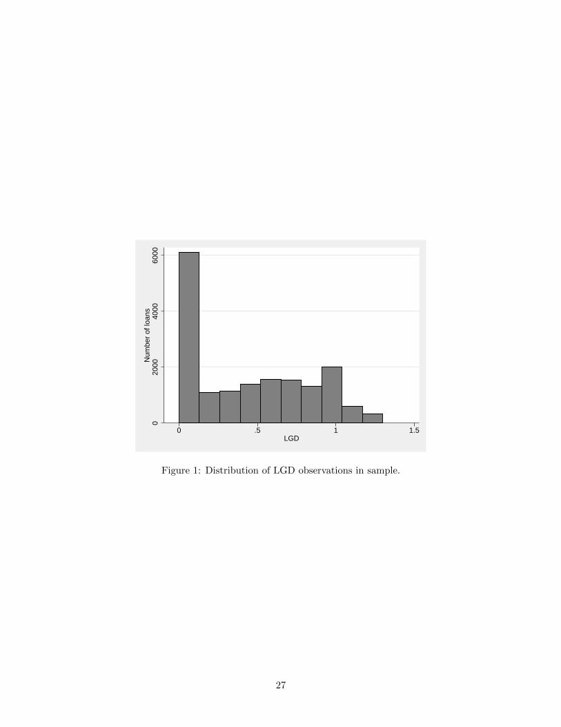
previous authors,23 we find a strong bimodal distribution for LGD, depicted in Figure 1. About 30

19A total number of 18,035 exclusions (56 percent) were made from a starting sample of 32,460 defaulted loanobservations. Of these 18,035 exclusions, 13,592 (75 percent) were made for censoring (most of these were assets thatwere still active). Another 2,691 (15 percent) of the exclusions lacked data for explanatory variables. Other reasonsincluded foreign assets (4 percent), loan size below $100 (4 percent) and data errors (2 percent).

20The nature of this censoring has both dependent and independent variable observations missing. These are notmissing relative to any particular threshold values. They are simply outside the snapshot of losses captured at thetime of loss share reporting. Censored or truncated regression modeling would not be suitable for these data.

21Five banks participated in the loss-share program but had no CRE loans.22The top five states are Florida, Georgia, Illinois, California and Washington.23See Asarnow and Edwards (1995), Araten, Jacobs, and Varshney (2004), and Schuermann (2004).

8

percent of the loans cured, and 10 percent had LGDs that exceeded 100 percent.

Because our sample is drawn from banks that failed during a severe recession, the results

should be interpreted with care.24 Banks rarely fail unless their portfolios have unusually high

default rates. Moreover, bank failures during the recent crisis were concentrated in geographic

regions that experienced higher-than-average economic distress. Of the 353 banks headquartered

in Georgia at year-end 2007, 87 (25 percent) failed by the end of 2013. None of the banks in North

Dakota failed.25 Despite the sample characteristics, our analysis supports the view that the LGDs

are generally comparable to other CRE bank loans during high-stress periods.26

3 Methodology

The approach we take is motivated largely by the empirical distribution of the LGD data. In Figure

1 we observe a large spike in the LGD distribution for defaulted loans with zero losses, after which

the frequency drops off dramatically. The abrupt spike on the far left tail suggests that the loans

with zero losses may behave differently from the rest of the defaulted loans. In his survey of the

LGD literature, Schuermann (2004) makes a similar observation: “Defaults resulting in 100 percent

recovery (0 percent LGD) are probably somewhat special and should be modeled separately. Put

differently, it is likely that there may be different factors driving this process, or that the factors

should be weighted differently.”27

With this in mind, we use a two-stage approach in our analysis. In the first stage we ask: What

factors influence the probability of a defaulted loan incurring losses? We assign LGD observations

into binary categories: loans having zero losses are set equal to 0; and loans that incur losses are set

equal to 1. Then we perform a logit regression on the probability of incurring a loss. In the second

stage we ask: Conditional on a defaulted loan incurring losses, what influences the loss severity?

We isolate the sub-sample of defaulted loans that experience losses and perform a linear regression

using their continuous LGD values. We then combine results from the two stages to examine the

marginal impact on expected LGD. Modeling the combination of loss probability and loss severity

in this way allows us to distinguish between drivers of LGD for defaulted loans that experience full

24Eighty-two percent of the loans in the sample were held by banks that failed in 2009 and 2010.25Source: FDIC.26See Shibut and Singer (2014) for additional discussion.27Schuermann (2004), 270.

9

recoveries and those that do not.

The expected value of LGD in our model is not a simple mean, but is weighted by the probability

of falling into either loss category:

E(LGD) =n∑

i=1

LGDi × πi + 0× (1− πi) (3)

where n is the number of defaulted loan observations, LGDi is the estimate of loss given default,

πi is the probability of loan i incurring a loss, and (1− πi) is the probability of loan i incurring no

loss. The probability πi of incurring a loss on the defaulted loan is computed from the logit model,

and the loss severity LGDi is computed from the linear regression model.28

Stage 1: Logistic regression with full sample

In the first stage, we examine what influences the probability of a defaulted loan in our sample

incurring zero versus non-zero losses. We separate the defaulted loans into two categories: those

with losses and those without losses. We have for outcome variable yi:

yi =

1 if defaulted loan i incurs a loss

0 if defaulted loan i has no loss

Then for yi = {0, 1}, the probability of observing realization yi from random variable Yi is:

Pr{Yi = yi} = πyii (1− πi)1−yi (4)

where πi is the probability that yi takes a value of 1 and (1 − yi) is the probability that it takes

a value of 0. The logit function takes the underlying probabilities for realization {y1, · · · , yn} and

28Leow and Mues (2012) use a similar approach to model LGD for residential mortgage loans. They have aprobability of repossession model to capture the likelihood of an account undergoing repossession given that it hasgone into default, and a haircut model to estimate the discount on the sale price of the repossessed property. Theformer is estimated with a logistic regression; the latter uses Ordinary Least Squares, or OLS.

10

links them to the linear predictor variables:

logit(πi) = log(πi

1− πi) = x′iβ (5)

where xi is the vector of covariates and β is the vector of regression coefficients. Solving for the

underlying probability πi of realization yi gives:

πi =exp{x′iβ}

1 + exp{x′iβ}(6)

The coefficients can be solved for via maximum likelihood.

Stage 2: Linear regression with loss sub-sample

In the second stage, we take the LGD loss sample and perform a linear regression. Conditional

on incurring losses, the LGD associated with defaulted loan i takes the form:

LGDi = β0 + x′iβ + εi (7)

where xi is again the vector of covariates and β is the vector of regression coefficients. This allows us

to examine the relationship between explanatory covariates and the severity of losses on these loans.

To control for bank-level fixed effects in our analysis, we use cluster-robust standard errors in

estimation.

4 Analysis

In this section, we describe the explanatory variables in our regressions and discuss our results.

11

4.1 Explanatory variables and expected effects

4.1.1 Loan characteristics

The defaulted loans in our sample are far smaller in asset size than those examined elsewhere in

the LGD literature. Our sample has a mean loan balance of $929,599 and a median loan balance of

$306,797 at the time of default. For comparison, Esaki et al. (1999) report a mean asset size of $4

million in their sample of CRE loans held by life insurers.29 The smallest loan reported by Gupton

et al. (2000) in their study of U.S. syndicated loans was $60 million.30 Ghent and Valkanov (2014)

report a mean size of $58 million for CMBS loans.31 Because certain collection costs are fixed or

semi-fixed, there is reason to expect that smaller loans would have higher LGDs. We therefore

include ln loan bal, or the log of the asset size at default, in our analysis.

We include several variables related to the seasoning of the loan at the time of default. First,

we include the age of the loan at default, age, to capture the observed tendency for worse quality

loans to default sooner. About 10 percent of the defaulted loans in our sample did so in the first

year, and 43 percent defaulted within the first three years.32 We include the squared term sq age

to allow nonlinear effects of age on LGD. In addition, we include pct remain, the percentage of the

original loan balance remaining unpaid at default. We expect loans that default early, with a high

percentage of the original balance remaining, to have higher LGDs. We also include a dummy for

loans already in default when the bank failed: default at failure. We expect a positive relationship

with LGD because we anticipate that the servicing quality is generally lower at failed banks than

at the acquiring banks and may result in worse recoveries.

A key way that banks differentiate loan quality at origination is through the interest rate

offered to the borrower.33 Because our sample includes loans originated in a variety of interest-rate

environments, we use the difference between the loan’s interest rate and the analogous Treasury

29Esaki et al. (1999), 80.30Their primary source is Moody’s, and their analysis covers commercial loans from 1989 through 2000. In the

appendix, they provide loan level information for defaults that occurred in 1999 and 2000; the $60 million is thesmallest figure reported there.

31They also report a mean size of $23 million for bank CRE loans, but their bank loan sample is not comparableto the sample in this paper because it excludes loans below $2.5 million.

32To check for the possibility that loan age is really capturing effects of loan vintage, we included dummies for yearof loan origination. We found that these were insignificant when added to the regression equation and did not changethe impact of loan age on LGD. It appears that our inclusion of the change in the commercial property price index(CPPI), between origination and extinction, cppi change, appears to effectively control for loan vintage effects.

33In fact, Morgan and Ashcraft (2003) find that interest rates align with asset quality more closely than with bankrisk metrics calculated at origination.

12

rate at origination.34 The mean interest-rate premium rate prem on these loans is 3.32 percent.

We expect LGD to increase as the interest-rate premium increases.

The workout period is an important indicator of both servicing quality (good servicers stay of

top of the assets and move promptly as needed) and origination quality (foreclosure takes time and

occurs more frequently for weaker credits). We include variables for the workout period (wkout),

the squared workout period (sq wkout), and a foreclosure dummy (foreclose). The mean workout

period is 6.12 quarters, and 29 percent of the loans in the sample were foreclosed.

In recognition of the additional costs associated with judicial foreclosure, we include a dummy

indicator for loans where the collateral is located in states that require judicial foreclosures (judi-

cial).35 We expect that judicial foreclosure will increase LGD, both for foreclosed loans (because of

increased expenses) and other loans with losses (because of stronger bargaining power for distressed

borrowers). As a result of potential complications in both the origination and servicing of loans

that are collateralized by assets outside of the bank’s geographic footprint, we include a dummy

indicator for out-of-territory loans (out territory). The definition follows that of the Community

Reinvestment Act, except that we base the designation on the collateral location rather than the

borrower location. We believe our paper is the first paper that provides empirical evidence on the

effect of judicial foreclosure and out-of-territory status on LGD.

We exclude lien status from the core regression on account of missing data for about 3,000

observations. However, we separately report the estimated effect of lien status on LGD in our

results section below. About 10 percent of the remaining loans had junior liens.

We lack data for several relevant items that are related to the origination process and have

been found in prior research to influence LGD. We do not have the original LTV, and thus we

cannot estimate the current LTV. We do not have net operating income for the collateral, and thus

cannot calculate the DSCR. We do not know the type of property (for example, multi-family or

office building); neither do we know the borrower’s industry. We also do not know about the extent

of the relationship between lender and borrower—that is, whether a bank made multiple loans or

provided other services to the borrower.

34For adjustable rate loans, the interest-rate premium is calculated as the loan interest rate at bank failure minusthe 1-year Treasury bill rate at bank failure. For fixed-rate loans, the premium is calculated as the loan interest rateminus the Treasury rate at origination for the Treasury note or bond with a term closest to the loan term.

35For observations where the collateral location is unknown but the borrower location is known, we assume thatthe borrower and the collateral are co-located. We follow the same treatment for all geographic areas.

13

4.1.2 Bank characteristics

Because banks of different sizes may differ in their resources for the origination and servicing of

loans, we include a variable for the log bank size, ln bank size. The mean failed bank size in our

sample is $805 million, and the median is $281 million. In addition, strong asset growth prior to the

demise of a failed bank could harm the origination and servicing capabilities of the bank. To test

for these effects, we include the average annual loan growth rate of the failed bank for the three-

year period leading up to the peak size of the failed bank: peak growth.36 We base this window

on regulator evidence concerning the life cycle of bank failures.37 We expect that both smaller

banks and banks that grew quickly before failure would face challenges in origination and servicing,

and thus would have higher LGDs. We also include the number of quarters that the bank had a

CAMELS rating of 4 or 5 during the period leading up to failure: delay close. Because failed banks

that experience serious distress for a long time are likely to face more serious resource constraints

than those that fail quickly, and because serious resource constraints might harm servicing quality,

we expect a positive coefficient.

We examined several other bank-level variables that were dropped because of insignificance. The

bank’s coverage ratio and its default rate at failure were expected to serve as further indicators of

bank origination and servicing quality. However, we did not find either of these to be significant in

our regressions. Dummy indicators for year of bank failure were also tested but were not significant.

We looked at business lines for the failed banks; however, most of the banks were classified as CRE

lending specialists and exhibited very little variation. We also examined de novo status, which we

found to be highly correlated with bank size and growth rates.

4.1.3 Market conditions

To gauge the overall market condition, we include the year-over-year change in the industry-wide

noncurrent rate for CRE loans at the time of default: industry nc.38 We also capture asset price

changes in commercial real estate from the Commercial Property Price Index (CPPI) published by

36For banks that shrank for a long period prior to failure, we use the growth rate leading up to failure. For veryhigh-growth banks, we cap the growth rate at 1000 percent; 21 banks exceeded the cap. Almost all of them were denovo banks.

37FDIC (1997). The three-year period was the shorter range observed for the bank failure life cycle; we also triedthe longer range of five years and found similar results.

38Source: FDIC calculations.

14

CoStar at the regional level. For this variable, we calculate the log change in the regional CPPI

(based on collateral location) between origination and the date when the asset was extinguished:

cppi change. The mean reduction in asset prices between origination and disposition is 20 percent,

and the median is even higher at 25 percent. Many of these properties suffered from very serious

asset price declines.

We examined several alternative macro-level variables that were not included in the final re-

gression. We looked at quarterly GDP, unemployment and personal income at the state level,

and regional dummy indicators. We examined other variables to capture real estate market condi-

tions, including the Real Estate Investment Trust (REIT) Equity Index, CMBS delinquency rates,

and the quarterly volume and average price of commercial property repeat sales provided by Real

Capital Analytics. Most of these were eventually left out of the regression equation because of

multi-collinearity, but a few (personal income and regional indicators) were dropped because they

lacked statistical significance.

Table 2 presents our explanatory variables in context of the primary factors (origination quality,

servicing quality, changes in property prices and market conditions, and seasoning) described in

the introduction. Table 3 provides their summary details.39

4.2 Regression analysis

Table 4 summarizes our regression findings. Column (1) shows the coefficient estimates from a

simple linear regression using the full LGD sample for comparison. We next categorize LGD as a

binary “loss” variable, where loss=0 for defaulted loans with zero losses and loss=1 for defaulted

loans with losses. We run a logit regression, with the coefficients shown in column (2) and their

marginal effects in column (3).40 In the second stage of the analysis we use a linear regression for

the sub-sample where loss=1. Column (4) shows these coefficients for loss severity. The last column

shows the predicted marginal impact at the mean for a one-unit change in each of the regression

variables. These are calculated by combining results from both logit and linear regression stages

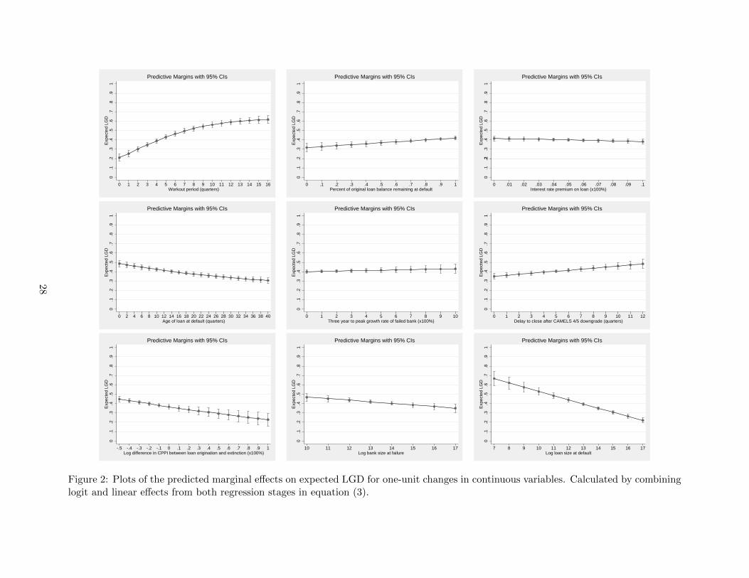
via equation (3). To improve the interpretation of various nonlinear relationships, Figures 2 and

39Variable correlations and variance inflation factors were also considered in determining the final regression spec-ification.

40We also estimate probit and complementary log-log functions as possible alternative linking formulations andfound that the results were not significantly changed.

15

3 provide predictive margins and confidence intervals for selected variables and combinations of

variables. Our findings from the two-stage analysis are largely consistent with the initial linear

regression. However, the two-stage methodology enables a deeper understanding of the covariate

impacts on LGD.

We find that a larger loan size at default is associated with lower losses, aligning with our

intuition regarding the probable effects of fixed or semi-fixed collection costs on smaller loans.

Other explanations for this phenomenon could be that the banks are more actively working the

largest of their defaulted loans for recoveries, or that the larger loans are made to higher-quality

borrowers with better chances for recovery. Other authors have found mixed results regarding

asset size.41 If fixed costs or resource allocation underlie the results, it is logical that the effect

would be stronger for our sample than for other studies that are based on larger assets. Loan size

matters in both the full and loss sample linear regressions, but it is not statistically significant in

the logit regression. This gives us a more nuanced interpretation of loan size effects with respect

to LGD. It does not appear to affect the probability of incurring losses. However, conditional on

loss=1, smaller loans are associated with a higher LGD. The effects are material, especially for

smaller loans: an increase in loan size from $100,000 to $200,000 is associated with a 311 basis

point reduction in LGD; a similar $100,000 increase from $1 million to $1.1 million is associated

with a 42 basis point reduction in LGD.

Consistent with the literature on effects of loan seasoning on the probability of default (PD),

we find evidence that loan seasoning relates to LGD. Loans defaulting soon after origination and

with higher proportions of unpaid balances remaining may be riskier or lower quality credits. This

influences both the likelihood of incurring losses as well as the loss severity. While the relationship

between loan seasoning and PD has been explored elsewhere, to our knowledge ours is the first

paper to show evidence for a relationship between loan seasoning and LGD. At the mean age of

just over four years, a one-quarter increase in the age of the loan at default is associated with a 47

basis point reduction in LGD. The effects are stronger early in the life of the loan: a one-quarter

increase at 1 year of age is associated with a 62 basis point reduction in LGD. The true marginal

effect might be lower than our measurement to the extent that loan seasoning is serving as a proxy

41Acharya, Bharath and Srinivasan (2003) find that size is generally not significant at emergence from bankruptcy,but is often significant for market prices at default. Schuermann (2004) concludes that asset size probably doesn’tmatter. Pendergast and Jenkins (2003) find that size matters for CMBS loans.

16

for origination or servicing quality effects. Loans with lower origination quality are likely to default

sooner. In addition, loans that defaulted before the originating bank failed also have higher losses,

suggesting that the servicing quality for those early defaults may have been weaker.

We also find that a higher percentage of the original loan balance remaining at default is

associated with a higher LGD. This may indicate that amortizing loans provide lenders a little

more safety than comparable balloon loans. The coefficient is significant in the logit regression but

is insignificant in the linear regression for the loss=1 sub-sample. It appears that the relationship

between high loan balances and LGD is driven more by the increased probability of incurring losses

than by the severity of the loss.

We considered—but rejected—the possibility that the loan seasoning variables might be serving

in some way as a channel of the relationship between default rates and LGD. We include the change

in the industry noncurrent ratio (industry nc) was to try to control for these effects.42 We therefore

think that the relationship between LGD and loan seasoning may indeed matter.

The interest rate premium is insignificant in the linear regression for loss severity, but the logit

regression suggests that a higher interest rate premium is associated with a lower probability of

incurring losses. This may reflect more prudent underwriting standards on some of these loans.

However, the effect of the interest rate premium on the probability of incurring a loss is small.

Workout period appears to matter a great deal: longer workout periods are related to higher

losses, indicating that the servicing quality is an important factor for LGD. Origination quality

may be relevant to this result as well, because inherently weaker credits are less likely to cure

quickly and more likely to be foreclosed. The non-linear workout term indicates that increases in

the length of the workout period probably matter most early in the workout process. This implies

that early efforts in the workout process for defaulted loans may be important for reducing losses.

The workout period is highly significant in both the logit regression and the loss sample regression,

affecting both the probability of incurring loss and the severity of loss. At a mean of 6.2 quarters,

a one-quarter increase in the workout period is associated with a 295 basis point increase in LGD.

The marginal effects are considerably stronger for workout periods of less than two years than for

longer workout periods, perhaps because cures generally occur shortly after default. The marginal

effects are weaker for loans in foreclosure. (See Figure 2.)

42We also tried the industry noncurrent ratio in levels and found results to be similar.

17

As expected, materially higher losses occur with foreclosures. The estimated marginal effect

under the two-stage model is a full 20 percentage points. These loans may be associated with

weaker underwriting, higher expenses, weaker markets and longer time lines.

The judicial foreclosure indicator is insignificant in the logit regression, but it is highly significant

for the loss sample. Having collateral in a judicial foreclosure state does not appear to affect the

probability of a full-recovery on the loan. Intuitively, the additional costs associated with foreclosure

would have no effect on loans that are strong enough to avoid losses. However, these additional

costs are associated with a substantially higher loss severity conditional on loss=1. The estimated

effect is an increase of 550 basis points in severity for loans incurring losses, and 392 basis points for

expected LGD when combined with the logit effects of an increased probability of incurring losses.

One might expect that judicial foreclosure influences LGD for loans where the collateral is

foreclosed but not for other troubled loans. To test this hypothesis, we try interacting the judicial

foreclosure indicator with foreclosure status to see whether foreclosed loans in judicial foreclosure

states have higher losses. We find that the coefficient on this interaction term is insignificant.

Borrowers may be able to seek more concessions from lenders in these locations because both

parties are aware of the additional cost and delay associated with judicial foreclosure. This in turn

would increase LGD regardless of whether foreclosure is undertaken.43

Consistent with what we think, loans made out-of-territory are associated with a higher LGD.

This may reflect a greater degree of asymmetric information with out-of-territory lending during

the origination or the servicing process (or both). This effect may also reflect a higher cost of

servicing these loans. The estimated marginal impact on expected LGD for out-of-territory loans

is 312 basis points.

The coefficient for bank size is significant in the logit regression but is insignificant in the loss

sample regression. Bank size is associated with the probability of loss, with smaller banks appearing

to have lower full-recovery rates. This lower rate could be explained in part by better resources at

larger banks for identifying and working problem credits. It may also that some of these smaller

banks accepted more credit risk at origination or lent outside of their core specialization areas in

the lead-up to the crisis. Bank size does not appear to affect the severity of losses, however. Taking

both the logit and linear regression results into account, we estimate that a $100 million marginal

43Judicial foreclosure (or location in a judicial foreclosure state) may also extend the workout period.

18

increase in bank size (at a median bank size of $281 million) is associated with a 51 basis point

reduction in LGD.

The bank’s asset growth prior to its demise is insignificant in our regression. However, there is

some collinearity of asset growth rates with bank size—smaller banks in our sample tend to have

higher growth rates. We also find that the significance of strong asset growth is affected by the age

of the loan as well as the inclusion of default-at-failure and out-of-territory dummy variables. In

other words, banks with higher growth rates appear more likely to have bad loans that defaulted

early, and they are more likely to have higher out-of-territory lending rates. Thus, the effect of

asset growth rates on LGD may already be captured through other aspects of the regression.

The length of time between being downgraded to a 4 or 5 CAMELS rating and bank failure is

not associated with whether losses occur in the logit regression. However, the time element does

have a positive relationship with loss severity for loans with loss=1. The relationship may indicate

a diminished capacity to manage seriously troubled assets, perhaps compounded by a desire to

delay the recognition of loan losses. This result also identifies a potential channel for increased

losses when regulators delay closure of problem banks. We estimate that a one-quarter lengthening

of the failed bank’s distress period at the mean of 4.82 quarters is associated with a 110 basis point

increase in LGD.

The change in the industry noncurrent rate is significant in both the logit and the loss sample

regressions, but their effects move in different directions. An increase in the industry noncurrent

rate is associated with a lower probability of incurring losses, but higher LGDs if losses occur. We

think that this may be a supply-side story—when the supply of defaulted loans is high, the market

may lower its valuation of the underlying collateral and thus greater losses may occur (hence the

positive effect in the loss sample). However, despite the higher incidence of noncurrent loans, many

of the better-quality borrowers may eventually be making good on their loans, resulting in a lower

probability of losses (hence the negative effect in the logit regression).

A decline in the CPPI between origination and the end of the workout period is associated with

higher LGDs. This provides evidence that losses are affected by changes in asset prices relative to

origination. The coefficient is negative and statistically significant in both logit and loss sub-sample

regressions, affecting both the probability of incurring loss and loss severity. The marginal effect is

smaller than one might expect: the predicted marginal effect of a 1 percentage point drop in CPPI

19

on LGD at the mean is 16 basis points.

Previous literature has found seniority status to be important for corporate bonds and larger

bank loans.44 When we include a dummy indicator for junior lien status, we see a significant and

positive relationship to LGD. The logit regression suggests that lien status does not influence the

probability of incurring losses, but the linear regression suggests that it is an important factor for

loss severity: it increases the marginal expected losses by over 800 basis points.

4.3 Robustness considerations

Since we differ from others in the literature by capping LGD at 130 percent rather than at 100

percent, we explore how this might affect our results. Around 10 percent of our sample of defaulted

loans exceeds 100 percent. For comparison, we run the same regressions by imposing a cap of 100

percent and find that our results change very little. It does somewhat lower the impact for some

of the explanatory variables—but not in a statistically significant manner. The mean LGDs only

change by around 1.5 percentage points.

We try dropping our largest failed bank from the sample. We find that the bank size effect

disappears from the full-sample linear regression, but remains significant in the logit regression.

This supports our two-stage conclusion that larger banks have a lower probability of incurring

losses, but do not necessarily appear to differ in the severity of the losses.

Another consideration is loan size. The majority of the loans in our sample are small, with 77

percent below $1 million and 87 percent below $5 million. However, there is a very long right tail

that extends to just over $45 million. Dropping the largest loans in the tail of the loan distribution

produces no significant change in the loan size effects on loss severity. For the logit model, we

observe that loan size is significant in influencing the probability of loss for loans below $1 million,

but is insignificant when loans up to $5 million and above are included. This suggests that loan

size categories or thresholds may have some bearing on LGD behaviors.

We try creating a category for the very smallest loans in our sample. Many of the higher LGDs

come from smaller loans, so we allow for the possibility that these small loans may be driving the

loan size effects on LGD. We include a dummy variable for loans having a balance of $100,000 or

less at default (about 20 percent of the sample). We find this dummy coefficient to be significant,

44See Acharya, Bharath and Srinivasan (2003) and Schuermann (2004), for example.

20

but the coefficient on loan size still matters. We therefore believe that the loan size effect on loss

severity is not being driven solely by high loss percentages on the smallest of the loans.

To test for the influence of regional factors on LGD, we try including regional dummies and find

that the coefficients on regional dummies are insignificant. Despite seeing geographic concentrations

in the data, there is not much unexplained regional variation in the results. The regional CPPI

index variable appears to have adequately captured the regional effects. Alternately, this result

may be partly explained by the broad reach of the recession during this time period, or because all

of the loans came from failed banks.

In addition, around 5.5 percent of our sample are loans from de novo banks. We include a

dummy indicator variable for de novo status, with the hypothesis that it is likely to be associated

with higher LGDs. The dummy is insignificant, but we do find that de novo status is correlated

with bank size and peak growth rates. Dropping these reveals a significant and positive influence

for de novo status in the logit regression. De novo status thus appears to matter for the probability

of incurring loss, but is otherwise captured through bank size and peak growth rate characteristics

in the regression.

5 Conclusion

In this paper we analyze a new dataset of over 14,000 defaulted CRE loans at 295 failed banks

during the recent financial crisis. We see several contributions of this study to the literature: 1)

We examine LGD for loans at small to mid-sized banks. Since the existing literature on LGD has

focused on large loans or bonds, and it is not known how applicable those results are to typical loans

at typical banks. 2) We provide new evidence suggesting a meaningful relationship between loan

seasoning and LGD. (Existing literature has focused on loan seasoning and probability of default

(PD).) 3) We identify certain bank-level characteristics that influence LGD. To our knowledge, no

other papers have examined bank factors affecting LGD. 4) Our two-stage approach reveals insights

that distinguish influences on the probability of loss and loss severity for LGD. 5) We find, as far

as we know for the first time in published research, empirical evidence of a relationship between

LGD and judicial foreclosure and out-of-territory lending. 6) We find a new potential channel that

could increase losses to the FDIC if regulators delay the closing of troubled banks.

21

We find evidence that the key factors that other authors have found to influence LGD for large

CRE loans tend to have similar effects on smaller CRE loans at failed banks. The length of the

workout period has a significant relationship with LGD, as does foreclosure. Lien status has a

strong effect, and changes in commercial property prices are important. Loan size has a stronger

relationship to LGD in our study than other authors—a characteristic possibly related to the effects

of fixed costs on a sample of loans that are much smaller than studied elsewhere. We estimate that

an increase in loan size from $100,000 to $200,000 is associated with a 311 basis point reduction in

LGD, and a $100,000 increase from $1 million to $1.1 million is associated with a 42 basis point

reduction in LGD. The channel appears to be a smaller severity of losses for loans that do not fully

recover (rather than the cure rate).

Although it is well known that loan seasoning influences default rates, the effect of loan seasoning

on LGD for commercial loans has largely been unexplored to date. We find evidence that loan

seasoning has a substantial effect on both the full-recovery rate and the loss severity for uncured

loans. At the mean, a one-quarter increase in the age of the loan at default is associated with a 47

basis point reduction in LGD. The effects appear to be somewhat larger for loans that default shortly

after origination. In addition, the share of the original loan balance that remains outstanding at

default is positively related to loss severity and negatively related to the odds of a full recovery. We

believe that risk measurement and stress testing at banks can be improved by incorporating loan

seasoning into LGD estimation. Supervisors should be aware that loan seasoning influences LGD

as well as PD when considering policies and procedures associated with high loan growth.

We find that CRE loans at small banks tend to have higher LGDs because they experience

lower full-recovery rates than larger banks. At the median, a $100 million increase in bank size

is associated with a 51 basis point reduction in LGD. It is unclear whether this effect relates to

differences in the underwriting or the servicing quality at these banks. It may be that larger banks

are better able to identify problem credits promptly, or small banks face difficulties in maintaining

a high-quality workout staff. This bank size effect could be explained in part by some of these

smaller banks lending beyond their core specializations in the lead-up to the crisis, or by a large

share of small banks being de novo banks with an immature infrastructure.

We are able to isolate the relationship of out-of-territory lending to LGD, and find that out-of-

territory loans tend to have moderately higher LGDs, probably because they present challenges in

22

both the origination and servicing functions. In addition, we find that judicial foreclosure regimes

do not influence the odds of experiencing losses, but are associated with a material increase in LGD

for loans that do experience a loss, regardless of whether foreclosure occurs. It appears that judicial

foreclosure may improve the distressed borrower’s position in negotiating with the lender.

For CRE loans with non-zero losses, we find that loss severity is positively related to the length

of time that banks remain in trouble prior to failure. The effects are material: a one-quarter delay

in bank closure at the mean is associated with a 110 basis point increase in LGD. The result points

toward a previously unexplored channel for increasing losses to the FDIC if the closing of troubled

banks is delayed. Troubled banks might experience increasing difficulties in maintaining servicing

quality as their problems persist. This finding supports prompt corrective action provisions for

troubled banks.

All of our results are based on a censored sample of loans from small and mid-sized banks that

failed in the midst of a major recession. Moreover, the loans are geographically concentrated, and

most of them defaulted in the middle of the recession. Therefore, our results should be interpreted

with care.

References

[1] Acharya, V., S. Bharath and A. Srinivasan, (2003), “Understanding the Recovery Rates of

Defaulted Securities,” CEPR discussion paper series, 2003.

[2] Altman, E., B. Brooks, A. Resti and A. Sironi, (2005), “The Link Between Default and Recovery

Rates: Theory, Empirical Evidence, and Implications,” Journal of Business 78, no. 6:2203–2227.

[3] Altman, E., A. Resti and A. Sironi, (2004), “Default Recovery Rates in Credit Risk Modeling: A

Review of the Literature and Empirical Evidence,” Economic Notes 2: 2004 Review of Banking,

Finance and Monetary Economics.

[4] Araten, M., M. Jacobs Jr. and P. Varshney, (2004), “Measuring LGD on Commercial Loans:

An 18-Year Internal Study,” The RMA Journal May 2004:28–35.

[5] Asarnow E. and D. Edwards, (1995), “Measuring Loss on Defaulted Bank Loans: a 24-Year

Study,” Journal of Commercial Lending March 1995:80–86.

23

[6] Bellotti, T. and J. Crook, (2012), “Loss Given Default Models Incorporating Macroeconomic

Variables for Credit Cards,” International Journal of Forecasting 28, no. 1:171–182.

[7] Bohn, E., (2009), “The Commercial Real Estate Workout: Strategies for Minimizing Losses in

a Troubled Market,” working paper.

[8] Brown, D.T., B.A. Ciochetti and T.J. Riddiough, (2006), “Theory and Evidence on the Reso-

lution of Financial Distress,” The Review of Financial Studies 19, no. 4:1357–1397.

[9] Carey, M. and M. Gordy, (2004), “Measuring Systematic Risk in Recoveries on Defaulted Debt I:

Firm-Level Ultimate LGDs,” FDIC: CFR Spring 2005 Research Conference Paper (Draft Memo).

[10] Cermele, M., M. Donato and A. Mignanelli, (2002), “Good Money from Bad Debt,” The

McKinsey Quarterly 2002, no. 1:103–111.

[11] Ciochetti, B.A., (1997), “Loss Characteristics of Commercial Mortgage Foreclosures,” Real

Estate Finance Spring 1997:53–69.

[12] Congressional Oversight Panel, (2010), “Congressional Oversight Panel February Oversight

Report: Commercial Real Estate Losses and the Risk to Financial Stability,” February 10, 2010.

[13] Esaki, H. and M. Goldman, (2005), “Commercial Mortgage Defaults: 30 Years of History,”

CMBS World Winter 2005:21–29.

[14] Esaki, H., S. L’Heureax and M. Snyderman, (1999), “Commercial Mortgage Defaults: An

Update,” Real Estate Finance Spring 1999:80–86.

[15] FDIC, (1997), History of the Eighties—Lessons for the Future: An Examination of the Banking

Crises of the 1980s and Early 1990s, 2 vols, FDIC.

[16] FDIC, (2012), FDIC Community Banking Study December 2012.

[17] FDIC Office of Inspector General, (2012), Evaluation of the FDIC’s Monitoring of Shared-Loss

Agreements, Office of Audits and Evaluations Report No. EVAL-12-002.

[18] Federal Register, (2007), “Risk-Based Capital Standards: Advanced Capital Adequacy

Framework—Basel II: Final Rule,” December 7, 2007:69287–69445.

24

[19] Felton, A. and J.B. Nichols, (2012), Commercial Real Estate Loan Performance at Failed U.S.

Banks, BIS Papers no. 64.

[20] Fitch, (2012), “CMBS 1.0...2.0...3.0...But Are We Progressing?,” www.fitch.com, January 4,

2012.

[21] Frye, J., (2000), “Depressing Recoveries,” Risk November 2000:108–111.

[22] Ghent, A. and R. Valkanov, (2014), “Comparing Securitized and Balance Sheet Loans: Size

Matters,” working paper.

[23] Gupton, G.M., D. Gates and L.V. Carty, (2000), “Bank-Loan Loss Given Default,” Moody’s,

November 2000:69–92.

[24] Hu, J. and R. Cantor, (2004), “Defaults and Losses Given Default of Structured Finance

Securities,” The Journal of Fixed Income March 2004:5–24.

[25] Hu, Y. and W. Perraudin, (2006), “The Dependence of Recovery Rates and Defaults,” Risk

Control Working Paper 6/1, February 2006.

[26] Kim, Y. (2014), “Modeling of Commercial Real Estate Credit Risks,” Quantitative Finance

13, no. 12:1977–1989.

[27] Leow, M. and C. Mues, (2012), “Predicting Loss Given Default (LGD) for Residential Mortgage

Loans: A Two-Stage Model and Empirical Evidence for UK Bank Data,” International Journal

of Forecasting 28:183–195.

[28] Moody’s, (2011), “Corporate Default and Recovery Rates, 1920-2010,” February 28, 2011.

[29] Moody’s, (2011), “Modeling Commercial Real Estate Loan Credit Risk: An Overview,” May

3, 2011.

[30] Morgan, D.P. and A.B. Ashcraft, (2003), “Using Loan Rates to Measure and Regulate Bank

Risk: Findings and an Immodest Proposal,” Journal of Financial Services Research 24, no.

2/3:181–200.

[31] Pendergast, L. and E. Jenkins, (2003), “CMBS Loss Severity Study: Portfolio Theory Aside,

Size Matters,” CMBS World Spring 2003:30–33,55–59.

25

[32] Shibut, L. and R. Singer, (2014), “Loss Given Default for Commercial Loans at Failed Banks,”

unpublished manuscript.

[33] Schuermann, T., (2004), “What Do We Know About Loss Given Default?” Credit Risk Models

and Management, ed. David Shimko, Risk Books:249–274.

26

020

0040

0060

00N

umbe

r of

loan

s

0 .5 1 1.5LGD

Figure 1: Distribution of LGD observations in sample.

27

.2.3

.4.5

.6.7

10

.1.8

.9E

xpec

ted

LGD

0 1 2 3 4 5 6 7 8 9 10 11 12 13 14 15 16Workout period (quarters)

Predictive Margins with 95% CIs

10

.1.2

.3.4

.5.6

.7.8

.9E

xpec

ted

LGD

0 .1 .2 .3 .4 .5 .6 .7 .8 .9 1Percent of original loan balance remaining at default


.4.3

.5.2

.61

.1.2

.7.8

.90

Exp

ecte

d LG

D

0 .01 .02 .03 .04 .05 .06 .07 .08 .09 .1Interest rate premium on loan (x100%)


01

.1.2

.6.7

.8.9

.3.4

.5E

xpec

ted

LGD

0 2 4 6 8 10 12 14 16 18 20 22 24 26 28 30 32 34 36 38 40Age of loan at default (quarters)


01

.1.2

.3.4

.5.6

.7.8

.9E

xpec

ted

LGD

0 1 2 3 4 5 6 7 8 9 10Three year to peak growth rate of failed bank (x100%)


01

.1.2

.3.4

.5.6

.7.8

.9E

xpec

ted

LGD

0 1 2 3 4 5 6 7 8 9 10 11 12Delay to close after CAMELS 4/5 downgrade (quarters)


.1.2

.3.4

.50

1.9

.8.7

.6E

xpec

ted

LGD

-.5 -.4 -.3 -.2 -.1 0 .1 .2 .3 .4 .5 .6 .7 .8 .9 1Log difference in CPPI between loan origination and extinction (x100%)


10

.1.2

.3.4

.5.6

.7.8

.9E

xpec

ted

LGD

10 11 12 13 14 15 16 17Log bank size at failure


.2.4

.6.8

10

.1.3

.5.7

.9E

xpec

ted

LGD

7 8 9 10 11 12 13 14 15 16 17Log loan size at default


Figure 2: Plots of the predicted marginal effects on expected LGD for one-unit changes in continuous variables. Calculated by combininglogit and linear effects from both regression stages in equation (3).

28

0.2

.4.6

.8E

xpec

ted

LGD


Foreclosure=0 Foreclosure=1


.2.3

.4.5

.6.7

Exp

ecte

d LG

D


Judicial foreclosure state=0 Judicial foreclosure state=1


.2.4

.6.8

Exp

ecte

d LG

D


Default at failure=0 Default at failure=1


.2.3

.4.5

.6.7

Exp

ecte

d LG

D


Out of territory loan=0 Out of territory loan=1


Figure 3: Plots of the predicted marginal effects on expected LGD for a change for dummy variable status xi = 0 to xi = 1. Calculatedby combining logit and linear effects from both regression stages in equation (3). Presented relative to workout period as a baselinetrajectory.

29

Mean LGD 43.78%Median LGD 41.06%Standard deviation of LGD 39.48%

Number of loans 17,116Aggregate loan balance at failure (in millions) $15,911Total number of failed banks 295

Distribution of loan balances at failure25th percentile $114,534Median $306,79775th percentile $869,104Mean $929,599

Concentration by bank (based on asset counts)% from largest bank 6%% from five largest banks 17%

Concentration by bank (based on asset balances)% from largest bank 7%% from five largest banks 25%

Concentration by location% from state with most failures (GA) 19%% from 5 states with most failures (GA,CA,FL,IL,WA) 65%

Table 1: Summary statistics.

30

Origination quality Servicing quality Property prices & Loan seasoningmarket conditions

Loan characteristicsSize of loan at default X XAge of loan at default X XPercent remaining balance at default X X XLoan in default at time of failure X X XInterest rate premium XWorkout period X X XProperty foreclosed X X XCollateral in judicial foreclosure state X XOut-of-territory loan X X

Bank characteristicsSize of bank at failure X XThree-year to peak asset growth rate X XRatings downgrading to failure X

Market conditionsChange in industry noncurrent rate XChange in CPPI XUnemployment rate X

Table 2: Explanatory variable factors influencing LGD within general classification framework.

31

Mean Median Std. Min Max

Loan characteristicsSize of loan at default $952,070 $314,055 $2,261,593 $103 $46,100,000Age of loan at default (in quarters) 16.29 14.18 11.48 0.011 126.91Percent remaining balance at default 0.867 0.954 0.215 0.0001 1.000Loan in default at time of bank failure (dummy) 0.267 0 0.443 0 1Interest rate premium 0.033 0.031 0.247 0 0.232Workout period (in quarters) 6.12 5.22 5.05 0 30.08Property foreclosed (dummy) 0.290 0 0.499 0 1Collateral in judicial foreclosure state (dummy) 0.473 0 0.499 0 1Out-of-territory loan (dummy) 0.316 0 0.465 0 1

Bank characteristics*Size of bank at failure (in thousands) $3,232,931 $896,864 $6,047,738 $18,155 $25,000,000Three-year to peak asset growth rate 1.17 0.657 1.84 -0.635 10.00Rating downgrade to failure (in quarters) 4.82 4.70 2.81 0 19.88

Market conditionsPctg. pt. change in industry noncurrent rate at default 0.846 0.997 1.29 -1.19 2.57Change in CPPI, loan origination to extinction -0.236 -0.287 0.188 -0.558 0.953Unemployment rate at time of default 0.097 0.100 0.017 0.032 0.142

Table 3: Explanatory variable summary statistics. *Calculated across loans in the sample, not across banks.

32

Coefficients Predicted marginLGD OLS-full Logit Logit-mfx OLS-loss (in percentage points)

(1) (2) (3) (4) (5)

ln loan size −0.039*** −0.031 −0.004 −0.064*** −4.42age −0.007*** −0.042*** −0.006*** −0.005*** −0.47

sq age 0.001*** 0.001** 0.001** 0.001pct remain 0.157*** 1.18*** 0.170*** 0.041 0.11default at failure 0.069*** 0.549*** 0.073*** 0.049*** 7.05rate prem −0.260 −6.46 *** −0.936*** 0.134 −0.34wkout 0.064*** 0.485*** 0.070*** 0.017*** 2.95

sq wkout −0.002*** −0.014*** −0.002*** −0.001foreclose 0.137*** 2.98*** 0.305*** 0.046*** 20.41judicial 0.023 0.042 0.006 0.055*** 3.92out territory 0.027** 0.255** 0.036** 0.022* 3.12

ln bank size −0.015*** −0.247*** −0.036*** −0.001 −1.68peak growth 0.004 0.044 0.001 0.01delay close 0.006** −0.012 0.002 0.016*** 1.10

industry nc 0.005 −0.162*** −0.023*** 0.038*** 0.01cppi change −0.189*** −1.55 *** −0.225*** −0.089** −0.16intercept 0.657*** 1.55 1.17***

No. observations 14425 14425 10030R-square .3679 .2282Pseudo R-square .3995Root MSE .3124 .2934

Table 4: Estimation results from (1) full sample linear regression, (2) logit regression estimating probability of nonzero losses, (3) logitregression marginal effects, (4) linear regression for loss severity conditional on nonzero losses and (5) combined marginal effect onexpected LGD from two-stage logit and conditional loss regressions. Marginal impacts for dummies calculated as a change from 0 to 1;all others calculated as a 1 unit change at the mean. For each margin calculation, the remaining variables are held constant at theirmean values. Separate squared-term marginal effects not shown as these are combined within the linear term marginal calculations.

33

Documents

What Drives Loss Given Default? Evidence from Commercial