UCD GEARY INSTITUTE

DISCUSSION PAPER SERIES

Modelling Downturn Loss Given Default

Raffaella Calabrese University of Milano-Bicocca

Geary WP2012/16 November 2012

UCD Geary Institute Discussion Papers often represent preliminary work and are circulated to encourage discussion. Citation of such a paper should account for its provisional character. A revised version may be available directly from the author.

Any opinions expressed here are those of the author(s) and not those of UCD Geary Institute. Research published in this series may include views on policy, but the institute itself takes no institutional policy positions.

Modelling Downturn Loss Given Default

Raffaella Calabresea

a University of Milano-Bicocca, Milan, Italy

Abstract

Basel II requires that the internal estimates of Loss Given Default (LGD)

reflect economic downturn conditions, thus modelling the “downturn LGD”.

In this work we suggest a methodology to estimate the downturn LGD dis-

tribution. Under the assumption that LGD is a mixture of an expansion and

a recession distribution, an accurate parametric model for LGD is proposed

and its parameters are estimated by the EM algorithm. Finally, we apply

the proposed model to empirical data on Italian bank loans.

Keywords: Downturn LGD; Mixed random variable; Mixture; Beta density

1. Introduction

The Basel II Accord (Basel Committee on Banking Supervision (BCBS),

2004, paragraph 286-317) considers the “Loss Given Default”(LGD) as the

loss quota in the case of the borrower’s default. In this framework, banks

adopting the advanced Internal-Rating-Based (IRB) approach are allowed

to use their own estimates of LGDs. Basel II requires that the internal

estimates reflect economic downturn conditions wherever necessary to cap-

ture risk accurately (BCBS, 2004, paragraph 468). Moreover, banks must

∗Corresponding author. Tel.: +39 02 64483193; fax: +39 02 64483105.Email address: raffaella.calabrese1@unimib.it (Raffaella Calabrese)

Preprint submitted to Elsevier November 23, 2012

account for the possibility that the LGD may exceed the weighted average

value when credit losses are higher than average, thus modelling the so-called

“downturn LGD”. In the assessment of capital adequacy the downturn LGD

is also useful for stress testing purposes (BCBS, 2004, paragraph 434). Al-

though the need to estimate the downturn LGD is clearly framed (BCBS,

2005), Basel II does not provide a specific approach that banks must use in

calculating this variable.

The main aim of this paper is to propose an accurate model for LGD

that allows to estimate the distribution function of the downturn LGD. We

consider a dynamic behaviour of LGD over the economic cycle characterized

by two regimes: expansion and recession. We assume that the LGD is a

mixture of an expansion and a recession distribution. Under the assumption

introduced by Calabrese (2012) in the regression framework, the expansion

and the recession distributions of the LGD are assumed to be two mixed

random variables, each of them is given by the mixture of a Bernoulli random

variable and a beta random variable. On the one hand, the Bernoulli random

variable allows to reproduce the high concentration of data on LGDs at total

recovery and total loss (Calabrese and Zenga, 2010; Renault and Scaillet,

2004; Schuermann, 2003). On the other hand, the beta distribution is well

suited to the modelling of LGDs (Gupton et al., 1997; Gupton and Stein,

2002), as it has support [0,1] and, in spite of requiring only two parameters,

is quite flexible.

To estimate the parameters of the LGD distribution, we apply the EM

algorithm. To obtain a finite beta density function, Calabrese and Zenga

(2010)’s parametrization is used. The suggested methodology allows to es-

timate the distribution of the downturn LGD and finally is applied to a

comprehensive survey on loan recovery process of Italian banks.

2

The present paper is organized as follows. The next section presents

the approach, here proposed, to estimate the downturn LGD distribution.

Section 3 describes the dataset of the Bank of Italy and shows the estimation

results by applying the proposed model to these data.

2. A model for downturn LGD

Two different distributions of LGDs are considered to hold over expan-

sion and recession periods, so LGDs can be seen as realization of these two

distributions. By considering two regimes of the economic cycle, expansion

and recession, LGDs are drawn from a mixture of an expansion (E) and a

recession (R) distributions

FLGD(lgd) = πFLGD/E(lgd) + (1− π)FLGD/R(lgd), (1)

where FLGD/S(lgd) is the cumulative distribution function of the LGD over

a given period conditional on the state S (S = E,R) of the economic cycle

and π is the probability of the expansion regime (Filardo, 1994).

Since the incidence of LGDs equal to 0 or 1 is high (Renault and Scaillet,

2004; Schuermann, 2003), to supply accurate estimations for the extreme val-

ues, Calabrese (2012) propose to consider LGD as a mixed random variable,

obtained as the mixture of a Bernoulli random variable and the beta ran-

dom variable B. This means that the distribution function of LGD FLGD/S

conditional on the state S of the economic cycle is defined as

FLGD/S(lgd) =

ps0 lgd = 0

ps0 + [1− ps0 − ps1]FB/S(lgd) lgd ∈ (0, 1)

1 lgd = 1

(2)

3

where FB/S denotes the distribution function of the beta random variable B

conditional on the state S of the economic cycle and psj = P{LGD = j/S}

is the conditional probability that the LGD is equal to j with j = 0, 1 given

the state S of the economic cycle.

The probability density function of the beta random variable B given S

of parametersθs

σs+ 1 and

1− θs

σs+ 1 is

gB/S(lgd; θs, σs) =Γ(θs

σs + 1)

Γ(1−θsσs + 1

)lgd

θs

σs (1− lgd)1−θsσs

Γ(θs

σs + 1, 1−θs

σs + 1) , (3)

where 0 < lgd < 1, 0 < θs < 1 is the mode of the beta density function and

σs > 0 is the dispersion parameter. The parametrization of the beta density

function gB/S(lgd; θs, σs) is applied by Calabrese and Zenga (2010) in the

nonparametric framework. The main advantage of this parametrization is

that the beta density function is finite for all values of θs and σs since the

beta parameters θs

σs + 1 and 1−θsσs + 1 are higher than one.

The beta random variable B given S of parameters θs

σs + 1 and 1−θsσs + 1

has an expected value

E(B/S) =θs + σs

2σs + 1

and variance

V (B/S) =σs[θs − (θs)2 + σs + (σs)2]

(1 + 2σs)2(1 + 3σs). (4)

To understand the influence of the parameter σs, we apply Maclaurin

series to equation (4) obtaining

V (B/S) = σsθs(1− θs) +O[(σs)2],

this means that the variance V (B/S) increases by increasing σs and main-

taining constant θs.

4

Assuming the states S of the economic cycle are unobserved, the prob-

ability π and the parameters (p0,p1,θ,σ) need to be estimated, where

p0 = [pe0, pr0]′, p1 = [pe1, p

r1]′ θ = [θe, θr]′ and σ = [σe, σr]′.

2.1. Calibrating the downturn LGD distribution

We use the Expectation-Maximization (EM) algorithm (Dempster et al.,

1977) to estimate the parameters π and (p0,p1,θ,σ).

In the mixture framework, the observed data lgd = (lgd1, lgd2, ..., lgdn)

is completed with a component-label vector Z = (Z1, Z2, ..., Zn) whose ele-

ments are assumed to be independent and are defined as

zis =

1 if lgdi comes from the state s

0 otherwise.

Under the assumption that LGDi are independent and identically dis-

tributed random variables with cumulative distribution function (1), the

complete-data log-likelihood function is

lc (π,p0,p1,θ,σ) = lnπ

n∑i=1

zie + ln(1− π)

n∑i=1

zir (5)

+

n∑i=1

∑S=e,r

zis ln fLGD/S (lgdi; ps0, p

s1, θ

s, σs) .

The EM algorithm iteratively maximizes the log-likelihood function (5).

Each iteration of the EM algorithm includes the E-step, which computes

the conditional expectation of the complete-data log-likelihood (5) given

the observed data lgd, and the M-step, which obtains the maximum of the

complete-data log-likelihood function (5).

To compute the inital value π(0), analogously to Ji et al. (2005) we as-

sign the smallest 50% of lgdi to the expansion component and the others

5

to the recession component. Maximizing (5), we obtain the initial values

(p(0)0 ,p

(0)1 ,θ(0),σ(0)). The algorithm follows the sequence:

(1) On the (k + 1)-th iteration, the E-step requires the calculation of the

conditional expectation of the complete-data log-likelihood (5). Since

Z is non-observed data, z(k)is is replaced by the conditional expectation

of Zis given the observed data lgd and we consider the parameter

estimates (π(k),p(k)0 ,p

(k)1 ,θ(k),σ(k)) from the k-th iteration of the M-

step

z(k+1)is =

P (k)(S)fLGD/S

(lgdi; p

(k)s0 , p

(k)s1 , θ(k)s, σ(k)s

)fLGD

(lgdi;p

(k)0 ,p

(k)1 ,θ(k),σ(k)

)where P (k)(S) = π(k) for S = R, P (k)(S) = 1− π(k) otherwise.

(2) On the (k + 1)-th iteration, the M-step requires the maximization of

the complete-data log-likelihood function (5) with respect to π, p0,

p1, θ, σ replacing zis by zk+1is . Firstly, the updated estimates π(k+1),

p(k+1)0 , p

(k+1)1 are obtained as

π(k+1) =

n∑i=1

z(k+1)ie

n

p(k+1)sj =

]{LGDi = j/S}P (k+1)(S)

n

where j = 0, 1.

The updated estimates θ(k+1) and σ(k+1) are the solution of the fol-

lowing system ∂lc (π,p0,p1,θ,σ)

∂θ= 0

∂lc (π,p0,p1,θ,σ)

∂σ= 0

6

Since the updated estimates θ(k+1) and σ(k+1) do not have a closed-

form, they are obtained by using a nonlinear optimization algorithm.

The E-step and the M-step are alternatively repeated until the difference

between two consecutive values of the complete-data log-likelihood (5) is

negligible.

3. Empirical analysis

The Bank of Italy conducts a comprehensive survey on the loan recovery

process of Italian banks in the years 2000-2001. By means of a questionnaire,

about 250 banks are surveyed. Since they cover nearly 90% of total domestic

assets of 1999, the sample is representative of the Italian recovery process.

The database comprises 149,378 defaulted borrowers. We highlight that the

data concern individual loans which are privately held and not listed on the

market. In particular, loans are towards Italian resident defaulted borrowers

on the 31/12/1998 and written off by the end of 1999.

The definition of default the Bank of Italy chooses in its survey is tighter

than the one BCBS (2004, paragraph 452) proposes. The difference is given

by the inclusion of transitory non-performing debts.

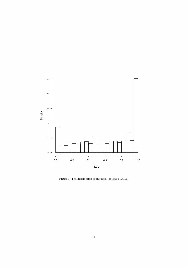
Figure 1 around here

To compute the LGD, we apply the expression proposed by Calabrese

and Zenga (2010). Figure 1 shows the Bank of Italy’s data. Firstly, the

mode of the LGD distribution is the extreme value 1, with 23% of the ob-

servations. Besides, LGD equal to 0 exhibits also a high percentage (7.78%).

The average LGD is 0.7158, the median value is 0.7777 and the standard

7

deviation is 0.3400.

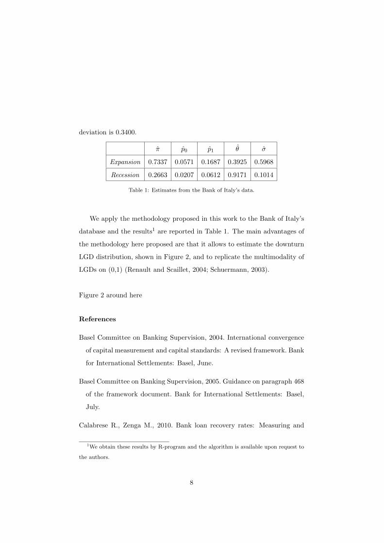
π̂ p̂0 p̂1 θ̂ σ̂

Expansion 0.7337 0.0571 0.1687 0.3925 0.5968

Recession 0.2663 0.0207 0.0612 0.9171 0.1014

Table 1: Estimates from the Bank of Italy’s data.

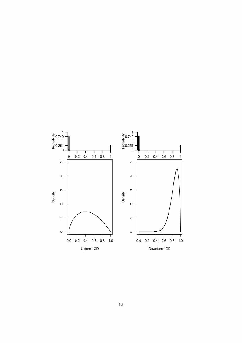
We apply the methodology proposed in this work to the Bank of Italy’s

database and the results1 are reported in Table 1. The main advantages of

the methodology here proposed are that it allows to estimate the downturn

LGD distribution, shown in Figure 2, and to replicate the multimodality of

LGDs on (0,1) (Renault and Scaillet, 2004; Schuermann, 2003).

Figure 2 around here

References

Basel Committee on Banking Supervision, 2004. International convergence

of capital measurement and capital standards: A revised framework. Bank

for International Settlements: Basel, June.

Basel Committee on Banking Supervision, 2005. Guidance on paragraph 468

of the framework document. Bank for International Settlements: Basel,

July.

Calabrese R., Zenga M., 2010. Bank loan recovery rates: Measuring and

1We obtain these results by R-program and the algorithm is available upon request to

the authors.

8

nonparametric density estimation. Journal of Banking and Finance 34(5),

903-911.

Calabrese R., 2012. Predicting bank loan recovery rates with mixed

continuous-discrete model. Applied Stochastic Models in Business and

Industry. To appear

Committee on the Global Financial System, 2005. The role of ratings in

structured finance: Issues and implications. Bank for International Set-

tlements: Basel.

Dempster A.P., Laird N.M., Rubin D.B., 1977. Maximum likelihood from

incomplete data via the EM algorithm (with discussion). Journal of the

Royal Statistical Society B 39(1), 1-38.

Filardo A. J., 1994. Business-cycles phases and their transitional dynamics.

Journal of Business and Economic Statistics 12 (3), 299-308.

Gupton G. M., Finger C. C., Bhatia M., 1997. CreditMetrics. Technical

document, J. P. Morgan.

Gupton G. M., Stein R. M., 2002. LosscalcTM : Model for predicting Loss

Given Default (LGD). Moody’s Investors Service.

Ji, Y. and Wu, C. and Liu, P. and Wang, J. and Coombes, K.R., 2005.

Applications of beta-mixture models in bioinformatics. Bioinformatics,

21(9), 2118-2122.

Renault O., Scaillet O., 2004. On the way to recovery: A nonparametric bias

free estimation of recovery rate densities. Journal of Banking and Finance

28, 2915-2931.

9

Schuermann T., 2003. What do we know about loss given default? Recovery

risk. Working paper, Federal Reserve Bank of New York.

10

LGD

Density

0.0 0.2 0.4 0.6 0.8 1.0

01

23

45

Figure 1: The distribution of the Bank of Italy’s LGDs.

11

0.0 0.2 0.4 0.6 0.8 1.0

01

23

45

Upturn LGD

Density

Probability

0 0.2 0.4 0.6 0.8 1

00.251

0.7491

0.0 0.2 0.4 0.6 0.8 1.0

01

23

45

Downturn LGD

Density

Probability

0 0.2 0.4 0.6 0.8 1

00.251

0.7491

12