Paper 141-2012 Building Loss Given Default Scorecard …support.sas.com/resources/papers/proceedings12/141-2012.pdf · Building Loss Given Default Scorecard Using Weight of ... We

1

Paper 141-2012

Building Loss Given Default Scorecard Using Weight of Evidence Bins in SAS® Enterprise Miner™

Anthony Van Berkel, Bank of Montreal and Naeem Siddiqi, SAS Institute Inc.

Abstract

The Credit Scoring add-on in SAS® Enterprise Miner™ is widely used to build binary target (good, bad)

scorecards for probability of default. The process involves grouping variables using weight of evidence,

and then performing logistic regression to produce predicted probabilities. Learn how to use the same

tools to build binned variable scorecards for Loss Given Default. We will explain the theoretical

principles behind the method and use actual data to demonstrate how we did it.

Loss Given Default

Loss Given Default (LGD) is defined as the loss to a lender when a counterparty (borrower) defaults. It is

one of the key parameters banks need to estimate for measurement of credit risk under the Internal

Ratings Based approaches specified by the Basel II accord – the other 2 measures being probability of

default (PD) and Exposure at Default (EAD). LGD is normally estimated as a continuous variable that

predicts the ratio of loss to balance at the time of default, with a range of 0 to 1.

Under Basel II scenarios, LGD is used to measure expected losses due to credit risk, which are eventually

used in the calculations of Risk Weighted Assets and ultimately, regulatory capital. In addition, LGD,

along with other measures is also used for measurement of economic capital and risk based pricingFor

Basel II risk measurement purposes, ‘default’ is generally taken as 90 days past due, however, other

definitions have also been used. The LGD is 100% minus the proportion of the balance at default

recovered by the lender during a workout period i.e. the period in which the lender tries to recover any

amount owed.

At a collateral level;

1___

cos__ecove%100;%0max

d

colcol

colhaircutpostvaluecollateral

tsworkoutamountryrLGD

Financial ServicesSAS Global Forum 2012

Building Loss Given Default Scorecard Using Weight of Evidence Bins in SAS® Enterprise Miner™ - Continued

2

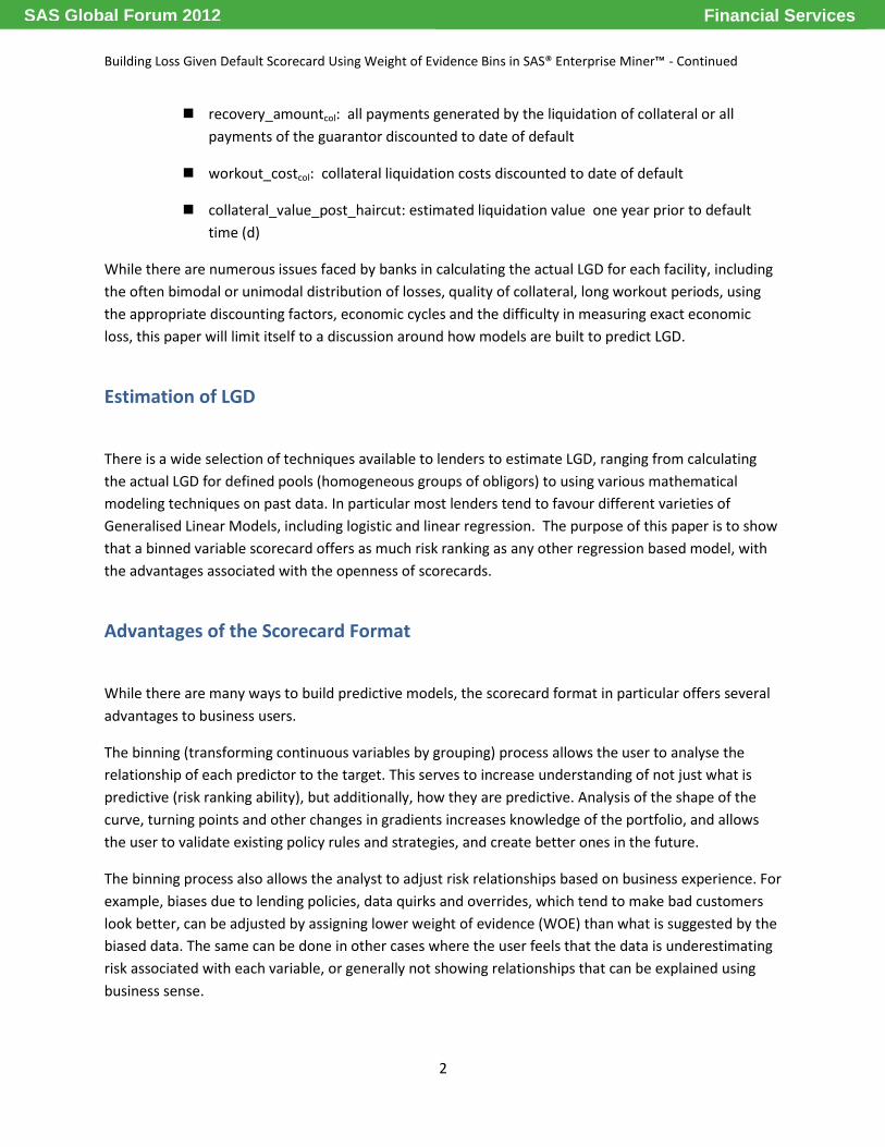
recovery_amountcol: all payments generated by the liquidation of collateral or all

payments of the guarantor discounted to date of default

workout_costcol: collateral liquidation costs discounted to date of default

collateral_value_post_haircut: estimated liquidation value one year prior to default

time (d)

While there are numerous issues faced by banks in calculating the actual LGD for each facility, including

the often bimodal or unimodal distribution of losses, quality of collateral, long workout periods, using

the appropriate discounting factors, economic cycles and the difficulty in measuring exact economic

loss, this paper will limit itself to a discussion around how models are built to predict LGD.

Estimation of LGD

There is a wide selection of techniques available to lenders to estimate LGD, ranging from calculating

the actual LGD for defined pools (homogeneous groups of obligors) to using various mathematical

modeling techniques on past data. In particular most lenders tend to favour different varieties of

Generalised Linear Models, including logistic and linear regression. The purpose of this paper is to show

that a binned variable scorecard offers as much risk ranking as any other regression based model, with

the advantages associated with the openness of scorecards.

Advantages of the Scorecard Format

While there are many ways to build predictive models, the scorecard format in particular offers several

advantages to business users.

The binning (transforming continuous variables by grouping) process allows the user to analyse the

relationship of each predictor to the target. This serves to increase understanding of not just what is

predictive (risk ranking ability), but additionally, how they are predictive. Analysis of the shape of the

curve, turning points and other changes in gradients increases knowledge of the portfolio, and allows

the user to validate existing policy rules and strategies, and create better ones in the future.

The binning process also allows the analyst to adjust risk relationships based on business experience. For

example, biases due to lending policies, data quirks and overrides, which tend to make bad customers

look better, can be adjusted by assigning lower weight of evidence (WOE) than what is suggested by the

biased data. The same can be done in other cases where the user feels that the data is underestimating

risk associated with each variable, or generally not showing relationships that can be explained using

business sense.



3

In some jurisdictions, a monotonic relationship is required between predictors and risk. The binning

process can be used to enforce this.

The format of the scorecard – each binned variable with assigned points – is extremely easy to

understand, explain and use. Reasons for low or high scores can be easily explained to regulators,

auditors and internal staff. This intuitive, business friendly format makes it easy to interpret, trouble

shoot and perform diagnostics when score distributions change. All of this makes it easier for scorecards

to get ‘buy in’ from end users compared to more complex models.

Building LGD Model Using WOE binned Scorecard

The data used for this project was from an overdraft portfolio at a major Canadian financial institution.

The actual dollar values were multiplied by a scalar to hide magnitudes . The accounts in the

development dataset were in good standing as of October 31, 2009, and defaulted within the following

year. These defaulted accounts were observed to the end of October 31, 2011 for ultimate loss, and the

LGD calculated as the ultimate loss divided by balance at original default point. The potential

explanatory variables selected for analysis came from performance on the overdraft account itself,

performance on other accounts held at the bank, possible updated bureau information obtained from

other accounts held at the bank and demographic data from the original application for the overdraft

product. All explanatory information is as of October 31, 2009 even though the default may have

happened up to 12 months after the point.

The base dataset consisted of 11,119 records, with 160 variables. Two datasets were created for the

purposes of this project, namely DATA100, and CLEANSED (explanations to follow).

The process we followed in building and benchmarking the scorecard consisted of the following main

steps:

a. We first converted the continuous LGD number for each account into a binary, resulting in the

duplicated data (DATA100)

b. Using the Interactive Grouping Node in SAS® Enterprise Miner™, we analysed the relationship to

WOE for each variable and binned the strong ones.

c. We built several logistic regression models and picked the best one, then converted it into a

scorecard format.

d. We validated the scorecard, and benchmarked its performance with a variety of other models

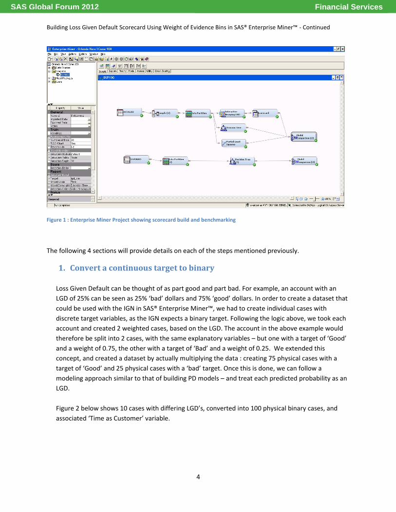
Figure 1 shows the EM project that was used in performing the steps mentioned above.



4

Figure 1 : Enterprise Miner Project showing scorecard build and benchmarking

The following 4 sections will provide details on each of the steps mentioned previously.

1. Convert a continuous target to binary

Loss Given Default can be thought of as part good and part bad. For example, an account with an

LGD of 25% can be seen as 25% ‘bad’ dollars and 75% ‘good’ dollars. In order to create a dataset that

could be used with the IGN in SAS® Enterprise Miner™, we had to create individual cases with

discrete target variables, as the IGN expects a binary target. Following the logic above, we took each

account and created 2 weighted cases, based on the LGD. The account in the above example would

therefore be split into 2 cases, with the same explanatory variables – but one with a target of ‘Good’

and a weight of 0.75, the other with a target of ‘Bad’ and a weight of 0.25. We extended this

concept, and created a dataset by actually multiplying the data : creating 75 physical cases with a

target of ‘Good’ and 25 physical cases with a ‘bad’ target. Once this is done, we can follow a

modeling approach similar to that of building PD models – and treat each predicted probability as an

LGD.

Figure 2 below shows 10 cases with differing LGD’s, converted into 100 physical binary cases, and

associated ‘Time as Customer’ variable.



5

Case LGD Goods Bads Time as customer

1 0.05 95 5 5

2 0.1 90 10 3

3 0.22 78 22 14

4 0.14 86 14 12

5 0.56 44 56 8

6 0.38 62 38 6

7 0.77 23 77 9

8 0.8 20 80 2

9 0.33 67 33 10

10 0.47 53 47 9

Total 3.82 618 382 Figure 2 : Process of converting a single case with calculated LGD into 100 'goods and 'bads'.

For the above example, average LGD is (3.82/10) = 0.382, while the ‘bad rate’ for the sample is

(382/(618+382)) = 38.2%.

Two datasets were created for this project. DATA100, with a total of 1,111,900 total cases, was built

by multiplying each good or bad by the LGD i.e. a case with an LGD of 20% would be converted into

20 bads and 80 goods. The reference dataset, CLEANSED, was created without physical

multiplication, with LGD based. Models built using both these datasets were compared at the end.

2. Perform WOE based binning, and select variables that showed sufficient

predictive power

We then used the Interactive Grouping Node in SAS® Enterprise Miner™ to analyse the predictive

power of each explanatory variable. Variables with low Information Value (IV) or Gini were discarded.

Those with IV of greater than 0.05 were then binned based on maintaining a reasonable IV, and

ensuring a logical relationship to the target. Variables that had strong predictive power, but whose

WOE curves were not explainable using business experience were discarded. This was done to ensure

that the final scorecard met the test of sanity from a business perspective, and to prevent any ‘buy

in’ issues.

The WOE calculation in SAS® Enterprise Miner™ is based on the standard formula below :

WOEbin = ln (proportion of Goods in bin/proportion of Bads in bin)

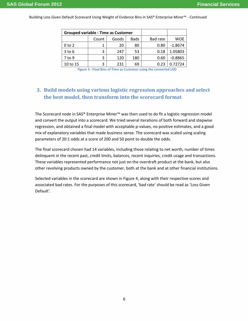
Using the data from Figure 2 above, the variable ‘Time as Customer’ would be binned as shown in

Figure 3.



6

Grouped variable : Time as Customer

Count Goods Bads Bad rate WOE

0 to 2 1 20 80 0.80 -1.8674

3 to 6 3 247 53 0.18 1.05803

7 to 9 3 120 180 0.60 -0.8865

10 to 15 3 231 69 0.23 0.72724 Figure 3 : Final Bins of Time as Customer using the converted LGD

3. Build models using various logistic regression approaches and select

the best model, then transform into the scorecard format

The Scorecard node in SAS® Enterprise Miner™ was then used to do fit a logistic regression model

and convert the output into a scorecard. We tried several iterations of both forward and stepwise

regression, and obtained a final model with acceptable p-values, no positive estimates, and a good

mix of explanatory variables that made business sense. The scorecard was scaled using scaling

parameters of 20:1 odds at a score of 200 and 50 point to double the odds.

The final scorecard chosen had 14 variables, including those relating to net worth, number of times

delinquent in the recent past, credit limits, balances, recent inquiries, credit usage and transactions.

These variables represented performance not just on the overdraft product at the bank, but also

other revolving products owned by the customer, both at the bank and at other financial institutions.

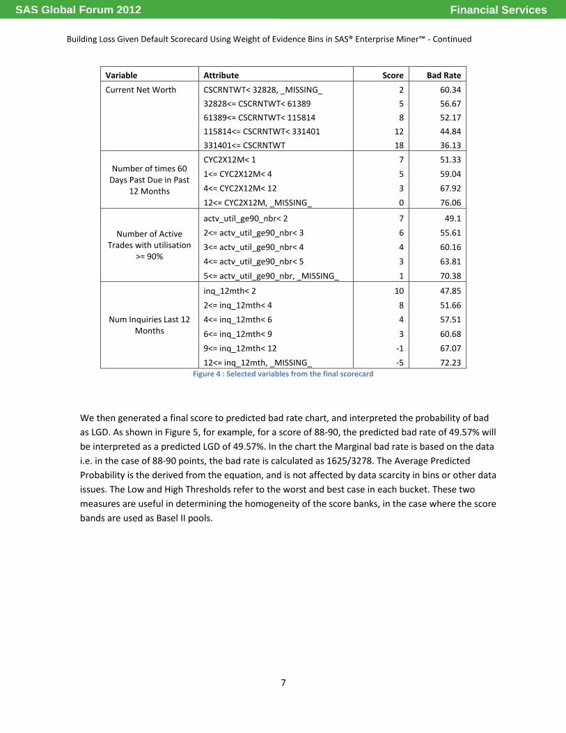
Selected variables in the scorecard are shown in Figure 4, along with their respective scores and

associated bad rates. For the purposes of this scorecard, ‘bad rate’ should be read as ‘Loss Given

Default’.



7

Variable Attribute Score Bad Rate

Current Net Worth CSCRNTWT< 32828, _MISSING_ 2 60.34

32828<= CSCRNTWT< 61389 5 56.67

61389<= CSCRNTWT< 115814 8 52.17

115814<= CSCRNTWT< 331401 12 44.84

331401<= CSCRNTWT 18 36.13

Number of times 60 Days Past Due in Past

12 Months

CYC2X12M< 1 7 51.33

1<= CYC2X12M< 4 5 59.04

4<= CYC2X12M< 12 3 67.92

12<= CYC2X12M, _MISSING_ 0 76.06

Number of Active Trades with utilisation

>= 90%

actv_util_ge90_nbr< 2 7 49.1

2<= actv_util_ge90_nbr< 3 6 55.61

3<= actv_util_ge90_nbr< 4 4 60.16

4<= actv_util_ge90_nbr< 5 3 63.81

5<= actv_util_ge90_nbr, _MISSING_ 1 70.38

Num Inquiries Last 12 Months

inq_12mth< 2 10 47.85

2<= inq_12mth< 4 8 51.66

4<= inq_12mth< 6 4 57.51

6<= inq_12mth< 9 3 60.68

9<= inq_12mth< 12 -1 67.07

12<= inq_12mth, _MISSING_ -5 72.23 Figure 4 : Selected variables from the final scorecard

We then generated a final score to predicted bad rate chart, and interpreted the probability of bad

as LGD. As shown in Figure 5, for example, for a score of 88-90, the predicted bad rate of 49.57% will

be interpreted as a predicted LGD of 49.57%. In the chart the Marginal bad rate is based on the data

i.e. in the case of 88-90 points, the bad rate is calculated as 1625/3278. The Average Predicted

Probability is the derived from the equation, and is not affected by data scarcity in bins or other data

issues. The Low and High Thresholds refer to the worst and best case in each bucket. These two

measures are useful in determining the homogeneity of the score banks, in the case where the score

bands are used as Basel II pools.



8

Score Bucket

Count

‘Bad’ Count

‘Good’ Count

Marginal Bad Rate

Average Predicted Probability

Predicted probability

Low Threshold High Threshold

Training Dataset

Score >= 107 4164 1262 2902 30.31 0.31 0.24 0.35

102 <= Score < 107 3807 1429 2378 37.54 0.36 0.33 0.40

98 <= Score < 102 4356 1741 2615 39.97 0.40 0.37 0.43

95 <= Score < 98 3942 1689 2253 42.85 0.43 0.41 0.46

93 <= Score < 95 3151 1402 1749 44.49 0.45 0.43 0.48

90 <= Score < 93 5216 2319 2897 44.46 0.47 0.44 0.50

88 <= Score < 90 3278 1625 1653 49.57 0.49 0.46 0.52

86 <= Score < 88 3706 1974 1732 53.26 0.51 0.48 0.54

84 <= Score < 86 3641 2012 1629 55.26 0.53 0.49 0.55

82 <= Score < 84 4004 2166 1838 54.10 0.54 0.51 0.57

80 <= Score < 82 3830 2141 1689 55.90 0.56 0.53 0.59

78 <= Score < 80 3556 2064 1492 58.04 0.58 0.55 0.61

75 <= Score < 78 5487 3172 2315 57.81 0.60 0.57 0.63

73 <= Score < 75 3068 1867 1201 60.85 0.62 0.59 0.64

70 <= Score < 73 4624 3033 1591 65.59 0.64 0.61 0.67

68 <= Score < 70 2821 1859 962 65.90 0.66 0.63 0.68

64 <= Score < 68 4538 3052 1486 67.25 0.68 0.64 0.72

60 <= Score < 64 3498 2501 997 71.50 0.71 0.68 0.74

54 <= Score < 60 3450 2646 804 76.70 0.74 0.71 0.77

Score < 54 3694 2886 808 78.13 0.80 0.75 0.89

Validation Dataset

Score >= 107 1772 562 1210 31.72 0.31 0.24 0.35

102 <= Score < 107 1697 662 1035 39.01 0.36 0.33 0.40

98 <= Score < 102 1944 785 1159 40.38 0.40 0.37 0.43

95 <= Score < 98 1717 733 984 42.69 0.43 0.41 0.46

93 <= Score < 95 1331 634 697 47.63 0.45 0.43 0.48

90 <= Score < 93 2227 997 1230 44.77 0.47 0.44 0.50

88 <= Score < 90 1355 663 692 48.93 0.49 0.46 0.52

86 <= Score < 88 1581 861 720 54.46 0.51 0.48 0.54

84 <= Score < 86 1520 824 696 54.21 0.53 0.49 0.55

82 <= Score < 84 1719 887 832 51.60 0.54 0.51 0.57

80 <= Score < 82 1674 938 736 56.03 0.56 0.53 0.59

78 <= Score < 80 1578 940 638 59.57 0.58 0.55 0.61

75 <= Score < 78 2284 1302 982 57.01 0.60 0.57 0.63

73 <= Score < 75 1303 790 513 60.63 0.62 0.59 0.64

70 <= Score < 73 1963 1273 690 64.85 0.64 0.61 0.67

68 <= Score < 70 1161 793 368 68.30 0.66 0.63 0.68

64 <= Score < 68 1980 1330 650 67.17 0.68 0.64 0.72

60 <= Score < 64 1541 1093 448 70.93 0.71 0.68 0.74

54 <= Score < 60 1503 1145 358 76.18 0.74 0.71 0.77

Score < 54 1509 1149 360 76.14 0.80 0.75 0.89

Figure 5 : Gains Table for Scorecard



9

4. Validate and Benchmark the Scorecard

The scorecard built was validated using various approaches on a 30% holdout sample. We compared

many fit statistics across the development and validation samples, and compared Kolmogorov-

Smirnov (KS) and ROC charts. Based on the results, some of which are shown in Figures 6 to 8, the

scorecard was deemed to be validated.

Figure 6 : Bad Rate by Score for Development and Validation Samples



10

Figure 7 : Cumulative Lift Chart for Development and Validation Samples

Figure 8 : ROC Curve for Development and Validation Samples



11

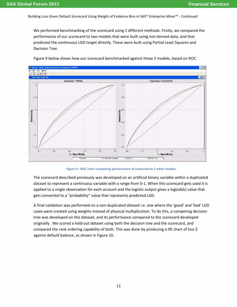
We performed benchmarking of the scorecard using 2 different methods. Firstly, we compared the

performance of our scorecard to two models that were built using non-binned data, and that

predicted the continuous LGD target directly. These were built using Partial Least Squares and

Decision Tree.

Figure 9 below shows how our scorecard benchmarked against these 2 models, based on ROC.

Figure 9 : ROC chart comparing performance of scorecard to 2 other models.

The scorecard described previously was developed on an artificial binary variable within a duplicated

dataset to represent a continuous variable with a range from 0-1. When this scorecard gets used it is

applied to a single observation for each account and the logistic output gives a log(odds) value that

gets converted to a “probability” value that represents predicted LGD.

A final validation was performed on a non-duplicated dataset i.e. one where the ‘good’ and ‘bad’ LGD

cases were created using weights instead of physical multiplication. To do this, a competing decision

tree was developed on this dataset, and its performance compared to the scorecard developed

originally. We scored a hold out dataset using both the decision tree and the scorecard, and

compared the rank ordering capability of both. This was done by producing a lift chart of loss $

against default balance, as shown in Figure 10.



12

Figure 10 : Comparing Rank Ordering Capabilities of models built using Duplicated and Unduplicated Data

This was done to satisfy a primary business concern at the bank. At this financial institution the main

concern for Basel II and business strategy is how well the model rank orders LGD. Accuracy is not the

primary concern for this financial institution - they simply want to identify who represents the worst

risk relative to default balance. A type of CAP curve is used to compare different models, such as the

graph above, which represents the proportion of the total loss captured against the proportion of

defaulted balance, on a dataset sorted by worst to best predicted LGD.

Discussion of Results and Conclusions

The scorecard had slightly lower fit statistics compared to direct prediction models, on the artificially

duplicated 100 times dataset. However, the scorecard was developed after its variables were



13

transformed from a continuous input into step functions, there was greater effort placed on business

sense in the transformation and getting a business optimal mix of variables into the final model. In our

opinion, having a scorecard that was more transparent and explainable to the business without

sacrificing too much predictive power is acceptable.

The scorecard, parts of which can be seen in Figure 4, represents a tool that can be used to easily

explain exactly what is contributing to high LGD’s and more importantly, how. The distribution of scores

make sense as they were binned with input from business experts who made decisions such as assigning

the worst scores to those with missing data. In addition, the mix of variables in the scorecard was

validated from a business perspective as representing what an experienced business analyst would think

of when determining default and loss given default. Note that this does not preclude experimentation to

find new predictive relationships – just that all relationships must be explainable in business terms.

Should this scorecard start assigning lower or higher points than what is expected, the source of this

deviation can be easily ascertained by checking average scores for each variable in the scorecard. Such

diagnostics become very difficult with more complex models that incorporate multiple interactions.

When decision making is the objective, being able to explain and diagnose always gets priority.

Even though the scorecard was developed on an artificially duplicated dataset, in reality it gets applied

to single observations, and the resulting predicted “probability of bad” value is taken as the effective

LGD. This is the scenario that we tested in the validation shown in Figure 5 where a raw sample was

scored using a competing decision tree and the scorecard. In terms of identifying the most loss $ for a

given amount of default $, the WOE scorecard appears to outperform the decision tree (as shown in

Figure 5). This rank order of loss is, as previously mentioned, more important to the bank than

calculated accuracy on the predicted loss or LGD value.

Based on this result, we conclude that the scorecard format, is firstly, producible for predicting LGD.

Secondly, its performance, while not equal to models that predict LGD directly, is of an acceptable level

for business purposes. In addition, based on the issues related to developing models on datasets that

are inflated via duplication (e.g. exaggerated Wald Chi-Sq), we would recommend that the IGN in

Enterprise Miner be enhanced to be able to calculate WOE for continuous targets. This would enable the

development of scorecards for purposes such as LGD and EAD, without data duplication, while

benefiting from the openness and flexibility of the scorecard format.



14

Bibliography

Chalupka R, Kopecsni J (2009): Modeling Bank Loan LGD of Corporate and SME Segments: A Case Study, Charles University in Prague, Faculty of Social Sciences, Czech Journal of Economics and Finance, 59, 2009, no. 4.

Resti A., Sironi A.: “Loss Given Default and Recovery Risk: From Basel II Standards to Effective Risk Management Tools”, The Basel Handbook (2004)

Arsova, M. Haralampieva, T. Tsvetanova, Comparison of regression models for LGD estimation, Credit Scoring and Credit Control XII 2011, Edinburgh 2011

Belloti, T. and Crook, J. (2007), “Loss Given Default models for UK retail credit cards”, CRC working paper 09/1

BCBS (2005): International Convergence of Capital Measurement and Capital Standards: A Revised Framework, Basel: Basel Committee on Banking Supervision – Bank for International Settlements, November 2005

Siddiqi, N. 2006. Credit Risk Scorecards: Developing and Implementing Intelligent Credit Scoring. New Jersey: John Wiley & Sons, Inc.

Peter Glößner, Achim Steinbauer, Vesselka Ivanova (2006), Internal LGD Estimation in Practice, WILMOTT magazine

SCHUERMANN, T. (2004): What Do We Know About Loss Given Default? New York: Federal Reserve Bank.

Contact Details

Your comments and questions are valued and encouraged. Contact the authors at: Anthony Van Berkel : [email protected] Naeem Siddiqi : [email protected] SAS and all other SAS Institute Inc. product or service names are registered trademarks or trademarks of SAS Institute Inc. in the USA and other countries. ® indicates USA registration.


mailto:[email protected]

Documents

Paper 141-2012 Building Loss Given Default Scorecard …support.sas.com/resources/papers/proceedings12/141-2012.pdf · Building Loss Given Default Scorecard Using Weight of ... We