..

TICAM REPORTJuly 1997

ERROR ESTIMATION AND ERROR CONTROLIN h-p FE APPROXIMATIONS OF

THE STOKES PROBLEM

J .Tinsley Oden and Serge Prudhomme

TEXAS INSTITUTE FOR COMPUTATIONAL AND APPLIED MATHEMATICSTHE UNIVERSITY OF TEXAS AT AUSTIN

..

ERROR ESTIMATION AND ERROR CONTROLIN h-p FE APPROXIMATIONS OF

THE STOKES PROBLEM

J .Tinsley Oden and Serge PrudhommeTexas Institute of Computational and Applied Mathematics

The university of Texas at AustinTaylor Hall TAY 2.400

Austin, TX, USA

Abstract

This paper deals with a posteriori error estimation for finite element approximations of the Stokesproblem. The ultimate objective is to analyse how given error quantities of interest are influenced bythe residuals, which are viewed as the sources of the numerical error. First, a global error estimator isproposed in terms of the norms of the residuals. Then, techniques to efficiently estimate these norms areadvocated. This is followed by the investigation of a general approach to evaluate the numerical error inpointwise, local or global quantities of interest.

1 Introduction

Error estimation in computational processes has been a subject of interest for more than two decades sincethe pioneering work of Babuska and Rheinboldt [3]. We refer to Ainsworth and Oden [2] and Verfiirth [19]for an extended account of the subject. In the particular case of the Stokes problem, several approacheshave been investigated in [18, 8, 6, 16, 2] .

The method we propose here belongs to the family of Implicit Error Residual Methods. The errors inthe velocity and pressure variables are driven by the residuals nh and n'j. in the momentum equationand the continuity equation respectively. The residuals represent the sources of error in the finite elementapproximations, and as such, are post-processed to provide meaningful error estimates in global "energy"norms. The evaluation of n'j. is shown to be exact, local and cheap. The calculation of the error measurenh is however more demanding. A new technique has been developed which provides accurate approxima-tions of nh through a global but inexpensive iterative process. First, error estimates are obtained usingspaces of low-order bubble functions as perturbations. These are then corrected by using enriched spacesconstructed through an adaptive procedure. This approach avoids the major difficulty of prescribing properboundary conditions for each subproblem in the Element Residual method [11, 7, 2]. The effectiveness ofthe methodology is demonstrated on various test cases of the Stokes problem with smooth and unsmoothsolutions.

In recent years, the success of a posteriori error estimation has prompted users to demand error estimatesin quantities of interest other than the classical energy norm. Works in this field have been undertaken byBabuska and Strouboulis [4] and Becker and Rannacher [10, 9] in order to estimate and control the errorby adapting the mesh parameters with respect to these quantities of interest. We extend the ideas to theStokes problem and perform a preliminary investigation of the performance of such techniques to evaluatethe error in pointwise, local or global quantities of interest.

1

2 Preliminaries

Let n denote an open bounded Lipschitz domain in IRn, n = 2 or 3, with boundary an. We consider theStokes equations:

with Dirichlet boundary condition:

-.6.u + \lp

\l·u

f in no in n (1)

u = g, on an, (2)

where u = u( x) and p = p( x) are respectively a vector-valued and a scalar-valued function defined at pointx = (Xl> X2, •.. ,xn) in n. Since the Stokes equations can be derived as a linearization of the steady-stateNavier-Stokes equations, the variable u and p are referred to as the velocity and pressure. The source termf = I(x) is a prescribed body force and 9 is a function defined on an which must satisfy the compatibilitycondition,

1g. nds = O.!an (3)

In what follows, we restrict ourselves to the case of homogeneous boundary conditions, i.e. 9 = 0 on an.This simplifies somewhat the theoretical analysis of the Stokes equations, while retaining all their interestingfeatures. We shall use standard notations for various Sobolev spaces of functions defined on n. We begin byintroducing the trial spaces of velocities V and pressures Q defined by:

V = H6(O) = (HJ(n))n

Q = {qEP(O):LqdX=O}

with corresponding norms:

Ivli = r \lv : \lv dxinIIqll~ = Lq2 dx.

We also introduce the bilinear forms a and b,

a: Hl(n) x Hl(O) ---t IR; a(u, v) = LV'u : V'v dx

b: Hl(O) x L2(O) ---t IR; b(v, q) = - L qV'. v dx.

The bilinear form a is the inner product associated to the norm 1.11 in V, so that

a(v, v) = lvii, T/v E v.

2

(4)

Lemma 2.1 The bilinear form b is continuous on V x Q, and in particular, there exists a positive constantMo such that

where Mo = vn, where n is the geometrical dimension of the problem.

Proof: Let v and q be arbitrary functions in V and Q. Since V' . v E Q, we have:

b(v, q) ~ 11\1· vllo IIqllo'

It is now sufficient to show there exists Mo such that IIV' . vllo ~ Mo Ivh. Indeed,

II" vll~ = In (t~::)'dx< r nt (~~;.)2dx

in ;=1 •

n in V'v: \1vdx

so that IIV' . vllo ~ vn Ivb and Mo = vn·

n Ivli.

o

Moreover, it can be shown that b satisfies the standard inf-sup condition (see Girault and Raviart [12]),i.e. there exists a constant /3 > 0 such that

•

sup Ib(v, q)1v E V\{O} Ivll ~ /3 IIqllo, T/q E Q.

The Stokes problem is now reformulated in the equivalent weak form:

For 1E V' given, find (u,p) E V x Q, such that

a(u, v) + b(v,p) = (I,v), T/v E V

b(u,q) = 0, T/q E Q

(5)

(6)

Extensive results concerning the existence, uniqueness and regularity of solutions (u, p) in V x Q of theStokes problem can be found in Girault and Raviart [12].

Let Vh C V and Qh C Q denote finite element spaces, possibly h-p finite element spaces [14],of thespaces V and Q. Approximate solutions to problem (6) are then obtained by solving the followingsystemof discrete equations:

For 1E V' given, find (Uh,Ph) E Vh x Qh, such that

a(uh' v) + b(V,Ph)

b(Uh,q)

3

(I, v), T/v E Vh

0, T/q E Qh

(7)

Let us consider a pair (Uh, Ph) E Vh X Qh, not necessarily a solution of (7). The numerical error(e, E) E V x Q in (Uh,Ph) is defined as

(8)

Then, substituting U and pin (6) by Uh + e and Ph+E respectively, we show that the distribution of (e, E)is governed by the system of equations:

aCe, v) + b(v, E)

b( e, q)

nf:(v), T/v E V

n'j. (q), T/q E Q(9)

where the linear functionals nf: : V ---t IR and n'j. : Q ---t IR

nf:(v)

n'j.(q)

(nf: ,v)

(n'j.,q)

(I,v)-a(Uh'v) -b(V,Ph)

- b(Uh, q)

are respectively the residual in the momentum equation and the residual in the continuity equation. Theresiduals nf: and n'j. are viewed as the sources of error. Indeed, whenever they are zero, the numerical erroris zero as well. A pointwise estimate of (e, E) could be obtained by approximating the following generalizedStokes problem:

Given nf: E V', 'R'j. E Q',

find (e, E) E V x Q, such that

a(e,v)+b(v,E) =b(e,q)

nf:(v), T/v E V

n'j. (q), T/q E Q

(10)

By virtue of Theorem 1.4.1 and corollaries in Girault and Raviart [12, p.61], a solution (e, E) exists and isunique. Since the residuals nf: and 'R'J., by definition, vanish on Vh and Qh respectively, whenever (Uh, Ph)is a solution of the finite system (7), approximations of (e, E) should be sought in finite element spaces largerthan the solution spaces Vh and Qh. In the next section, we show how the residuals can provide reliableglobal error estimates in specific norms.

3 Global Error Estimation

The objective here is to relate the residuals to the numerical errors expressed in some global norms. First,we recall (see Girault and Raviart [12, p.22]) that the space V = H5(n) can be decomposed into the directsum:

(11)

where the spaces J and Jl. are defined as:

J = {vEV; b(v,q) =0, T/qEQ}

Jl. = {v E V; a(v,w) = 0, T/w E J}

4

The space Jl. is the orthogonal complement of J with respect to H~(n) for the inner product a(·, .) associatedwith the norm 1.11, It follows that the error in the velocity variable e E V can be uniquely decomposed intoa sum of two vectors, ed E J and el. E Jl., such that

(12)

We naturally measure the error (e, E) in the usual global norm

and consider the following norms for the residuals nf: and n'j.

(13)

•1I"R.f:II. sup 1'Rf:(v)1

v E V\{O} Ivll

sup In'j.(q)1q E Q\{O} IIqllo

sup nf:(v)v E V\{O} Ivll '

sup n'j. (q)q E Q\{O} IIqllo .

(14)

Lemma 3.2 With the above definitions and assumptions:

(15)

..

Proof: From the definition of the residual n'j. and the continuity of the bilinear form b, we have, for allq E Q

The upper bound in (15) follows as

The divergence operator is an isomorphism of Jl. onto Q, so the function V' . el. belongs to Q and therefore

which yields

From Girault and Raviart [12, p.24, p.81], we obtain the lower bound in inequality (15) as

The lemma is proved.

5

o

Lemma 3.3 With the above definitions and assumptions, we have:

Proof:

1. By simple algebra, we get:

(1)(2)(3)

ledll ~ lI'R.hll.·IInhll. ~ jell + Mo IIEllo·13I1Ello ~ 11'R.'hII. + leJ.ll '

(16)(17)(18)

which shows (16).

2. We also have

a(ed, ed) = a(e, ed) = n'h(ed) - b(ed, E) = n'h(ed)

< IIn'hIl.ledll'

..

n'h(v) < a(e, v) + b(v, E)sup - supv E V Ivll - v E V Ivll

a(e,v) b(v,E)< sup -+ sup- v E V Ivll V E V Ivll< lell +Mo IIEllo .

3. The upper bound for the error in the pressure variable follows from the inf-sup condition on the bilinearform b, i.e.

b(v, E) b(v, E)13I1Ello ~ sup -II ~ sup -, I

v E V V 1 V E JJ. v 1

'R.'h(v) - aCe,v)< supv E JJ. Ivll

nmh(v) aCe, v)< sup -+ sup -

v E JJ. Ivll V E JJ. Ivllnm

h(v) a(eJ., v)< sup -+ supv E V Ivll V E JJ. Ivh

< IInhll. + leJ.ll .

o

Theorem 3.1 Let (e, E) be the numerical error in an approximation (Uh,Ph) of the Stokes problem. Thenthere exist positive constants Cl and C2 such that

6

(19)

where Cl and C2 depend only on the constants 13 and Mo respectively:

C1 = 1/2 min(l, 134),C2 = max(2 + M; ,2M;).

Proof: The proof of this theorem directly follows from Lemma 3.2 and Lemma 3.3. In particular, thelower bound is obtained from inequalities (15), (16) and (18), while the upper bound is derived from theinequalities (15) and (17). 0

This theorem is similar to the Theorem 6.1 introduced by Ainsworth and Oden in [2]. It shows that theglobal quantity IIn'j.lI: + IInf:lI: is equivalent to the global error measure lI(e, E)1I2. We emphasize that itrepresents a meaningful quantitative global estimate as long as the constants Cl and C2 do not take valuesfar from one. Here the constant C2 takes the value 4 in two-dimensions and 6 in three-dimensions sinceMo = vn. Therefore, the accuracy and robustness of this error estimate essentially depends on the value ofCl, a fortiori, 13, which depends itself on the problem in consideration. Moreover, we emphasize that such aglobal result does not provide any reliable information about the local (elementwise or pointwise) error, aswe know that the error can propagate far away from their sources nf: and n'j.. This actually motivated thework undertaken by Babuska, Strouboulis and co-workers [4]and Oden and Feng [15]on pollution error inorder to estimate the contributions of the residuals to the error outside the region of interest. However, thequantity IInf: II: + IIn'j.II: provides information about the location and intensity of the sources of errors, andas such, should be used to determine local refinement indicators.

4 Evaluating the Norms of Residual

This section is devoted to the evaluation of IInf: II. and IIn'j.II•. The objective is, on one hand, to minimizethe cost of the computations while retaining a certain accuracy, and, on the other hand, to obtain elementwisecontributions of these quantities.

4.1 Residual in the Continuity Equation

The residual n'j. gives us information about whether the discrete velocity Uh does or does not satisfy theincompressibility constraint. This is stated in the next lemma, where the norm of the residual 'R'j. is expressedin terms of the divergence of Uh.

Lemma 4.4 Let Uh E Vh be the velocity in the finite element solution of the Stokes problem. Then,

(20)

Proof: From the definition of the residual 'R'j. and the bilinear form b, we have, for all q in Q:

It follows that

(21)

7

We also have

that is, 11\1 . uhllo ::; IIn'hII., and the equality (20) has just been proven. o

The result of Lemma 4.4 is remarkable in the sense that the evaluation of IIn'hll. is both exact and cheap,as it is equivalent to compute the L2(n)-norm of the function V' . Uh. In addition, it is straightforward todecompose IIn'j.lI. into a sum of elementwise contributions as:

where LK represents the sum over all the elements in a finite element partition.

4.2 Residual in the Momentum Equation

Simple considerations reveal that the evaluation of Ilnf:ll. is neither cheap nor exact. At best, one obtainsapproximations of it. There exist basically two approaches to compute such approximations. The first onealways delivers lower bounds on IInf:lI. while the other provides upper bounds. Here we only consider theformer, which is called the conforming method.

4.2.1 Exact Evaluation

Since V is a Hilbert space, the Riesz Representation Theorem tells us there exists a unique element l{Jin Vwhich satisfies:

as well as:

a(l{J,v) = nf:(v), T/vE V, (22)

(23)

In other words, the residual nf: E V'is identified with an element l{JE V of equal norm. Moreover, thefunction l{Jgives information about the local intensity of the residual nf:, such as:

However, the problem (22) cannot be solved numerically due to the infinite dimension of the space V.

4.2.2 Conforming Finite Element Approximations

The objective here is to construct a finite element subspace yh C V, hence the label conforming method, inwhich to approximate problem (22), that is, to find l{Jh E yh such that:

(24)

8

We show that the norm of C{>h is always smaller than the norm nf: and that both quantities are indeedequivalent. First, we observe from (22) and (24) that:

(25)

In consequence, C{>h is simply the orthogonal projection of C{> onto the space Vh with respect to the innerproduct a(·,·) associated with the norm 1.11, It follows that:

(26)

which yields the following inequality:

(27)

Such a result can be sharpened, as stated in the next lemma.

Lemma 4.5 Let C{> E V and C{>h E vh satisfy (22) and (24) respectively. If C{> i= 0, let Vh be such thatC{>h i= O. Then, there exists a constant (J", 0 ~ (J" < 1 such that:

(28)

o

Theorem 4.2 Let C{> E V, C{>h E Vh and Vh satisfy the conditions of Lemma 4.5. Then, there exists aconstant (J", 0 ~ (J" < 1, such that:

(29)

Proof: The upper bound follows from equality (26). Indeed,

Now, making use of (26) and (28), we have:

that is

from which the lower bound follows.

(30)

o

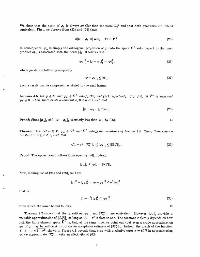
Theorem 4.2 shows that the quantities lC{>hll and /Inf:lI. are equivalent. However, lC{>hll provides avaluable approximation of IInf: II. as long as viI - (J"2 is close to one. The constant (J" clearly depends on howrich the finite element space Vh is, but, at the same time, we point out that even a crude approximationC{>h of C{> may be sufficient to obtain an acceptable estimate of IInf:II." Indeed, the graph of the functionf : (J" --+ J1- (J"2, shown in Figure 4.1, reveals that, even with a relative error (J" = 60% in approximatingC{>, we approximate IInf:lI. with an effectivity of 80%.

9

10.80.6x

0.40.2

............ ;......... : ---.........~ . /, K: /1

0.8

0.6X-- 0.4

0.2

00

Figure 4.1: Graph of f(x) = (1 - X2)1/2.

The finite element space yh has to be chosen so that the action of the residual nf: is different from zerofor at least one element of Yh. In the case where the pair (Uh, Ph) is the solution of problem (7), we observethat the residual vanishes on Vh

, that is:

nf:(V) = 0, T/v E Vh. (31)

It follows that the space yh should be larger than Vh itself. It is then constructed by enriching Vh withelements of a space Wh

, called space of perturbations, which satisfies

(32)

so that:

(33)

Since Vh C yh, problem (24) is more expensive to solve than the original one. At this point, we want toreduce the cost of the computations by taking advantage of the fact that the residual vanishes on the spaceVh. In other words, we would like to approximate 1I'Rf:II. by the norm of the function "ph E Wh satisfying

(34)

Following Bank [5], we suppose that a Strengthened Cauchy-Schwartz Inequality holds with respect tothe spaces Vh and Wh, in the sense that there exists a positive constant 1 < 1 such that for all Vh E Vhand for all Wh E Wh,

(35)

which implies, using Young's inequality, that

IVh+whli = IVhli+2a(vh,wh)+lwhli

> IVhli - 21 IVhlllwhll + IWhii> IVhli -Ivhli - 12

1whli + IWhii> (1 - 12) IWhii .

10

Thus,

(36)

The Strengthened Cauchy-Schwartz Inequality allows us to relate the accuracy of the approximation I?p h 11 ~

l<Phb to -y, the cosine of the angle between the spaces Vh and Wh:

Theorem 4.3 Let <PE V, <Ph E Vh and Vh satisfy the conditions of Lemma .{5. Let the strengthenedCauchy-Schwartz inequality (35) hold for the spaces Vh and Wh, where Vh = Vh + Wh and nf: = 0 onVh. Let ?Ph E wh satisfy (34). Then

(37)

...Proof: The upper bound is readily obtained as wh C V. In order to prove the lower bound, we write<Ph= <Pi.+ 1/7i., where <Pi.E Vh and 1/7i. E Wh. Then, from equation (24), we have, since <Pi.E Vh:

(38)

and from (24) and (34), we get:

Hence,l<phli = a(<Ph, <Ph) = a(<Ph, <P'h+ 1/7'h)= a(<Ph, 1/7'h)= a(1/7h, 1/7'h)

< l1/7hlll1/7'hll'

Applying the strengthened Cauchy-schwartz inequality to solution <Phyields:

which, combined to (40), gives

that is,

Then, using inequality (30) shown in Theorem 4.2, allows us to write:

The lower bound is proved.

(39)

(40)

(41)

(42)

(43)

o

The above theorem shows that the accuracy of the approximation l1/7hll ~ 1<pll only depends on theconstants (]"and -y.

11

We recall that (j depends on the richness of the space Vh, or Wh. The main difficulty is to construct Wh

so that the approximations tPh E l-Vh deliver reliable estimates of IInf:lI* at the lowest cost. In h-p finiteelement methods, the perturbations can be conveniently constructed from layers of piecewise polynomialbasis functions involving monomials of degree between p + 1 and p + q, q ~ 1, where p is defined as themaximal degree of the basis functions in Vh

. Obviously, in two-dimensional problems, such basis functionsconsist of edge and/or interior bubble functions. In three-dimensional problems, they would consist of edge,face and/or interior bubble functions. One question one has to answer is "what is the best value for q ?"Actually, this is problem dependent, and one should consider a method in which the value of q is increasedas needed.

We recall that "Y represents the angle between Vh and Wh. Its value is directly related to the choice

of the shape functions used to construct the basis functions of Vh and Wh. Here we use hierarchic shapefunctions based on integrated Legendre polynomials (see Szabo and Babuska [17, chapt. 6]), which satisfythe orthogonality property with respect to the inner product a(-, .).

Meanwhile, the cost in solving (34) is controlled by the dimension of Wh. However, the bilinear form

a(·, .) is symmetric and positive definite so that the finite system (34) can be cheaply solved using theiterative Conjugate Gradient method (CG). Moreover, we emphasize that the solution does not have to behighly accurate as we are interested in an estimate of the error, so that it is usually sufficient to perform afew iterations.

Finally, conforming methods always deliver lower bounds on nf:. In order to construct upper bounds,one has to approximate problem (22) in a space larger than V. This lead to the equilibrated residual methoddeveloped by Ainsworth and aden [1, 2] or Ladeveze and Leguillon [13]. In this approach, the globalproblem (22) is decoupled into a collection of local problems, usually constructed on each of the elements inthe partition. Our present conforming method avoids the major difficulty of prescribing boundary conditionsfor each subproblem typical of the equilibrium methods at comparable cost.

5 Estimation and Control of Error Quantities of Interest

Let L denote a linear functional defined on the product space V x Q. We suppose that we are interested inthe error quantity L(e, E) E IR, which we want to estimate and control. For example, L(.,.) may representsomething more localized than the global estimate (19), such as the error in u and p or their gradients ata point Xo E n or along a curve reO; e.g. L( e, E) = E( xo) or L( e, E) = §r e . n ds, etc. We cite moreexamples later. The main objective is then to relate L(e, E) to the sources of error nf: and n'j.; in otherwords, we would like to find linear functionals wm and wC

, if they exist, such that

..

(44)

These functions are viewed as influence functions (analogous to Green's functions) as they indicate theinfluence of the residuals on the quantity L(e, E). They are defined on the bidual of V and Q, and sincethese spaces are reflexive, we have:

(45)

(46)

This is understood in the sense that for each wm E V" and each wC E Q", there exist (;jm E V and wC E Qrespectively such that

(47)

12

(48)

By identifying &1m and WC with wm and WC respectively, the relation (44) becomes

(49)

Substituting for the terms nf:(wm) and n'j.(wC) in (49) using (9), rearranging and assuming a symmetric,

we finally get

L(e, E) a(e,wm) + b(wm, E) + b(e,wC)

a(wm, e) + b(e,wC) + b(wm, E).

(50)

(51)

It follows that the influence functions can be obtained as solutions of the global dual problem:

• Find (wm ,WC) E V x Q, such that

a(wm, v) + b(v,wC) + b(wm, q)

which is equivalent to the generalized Stokes problem:

Find (wm, WC) E V x Q, such that

a(wm, v) + b(v,wC)

b(wm,q)

L(v, q), T/(v, q) E V x Q

L(v,O), T/v E V

L(O, q), 'rIq E Q

(52)

(53)

It readily follows that the functions wm and WC do exist and are unique as L(v,O) E V' and L(O, q) E Q'(see Girault and Raviart [12]). Obviously, (53) cannot be solved exactly for the functions wm and WC in thegeneral case. At best, one seeks numerical approximations of wm and WC• This raises two questions, whichshould be simulatenously investigated:

1. How do we effectively calculate finite element approximations of wm and WC? In particular, is itnecessary to solve a global problem?

2. How do we utilize the relation (49) to derive elementwise refinement indicators in order to control theerror quantity L(e, E) ?

From a computational point of view, we observe that the cost involved in approximating wm and WC inthe spaces Vh and Qh is almost negligible, as the resulting finite system has already been factorized onceto calculate the solution (Uh, Ph). The cost therefore reduces to perform one backward and one forwardsubstitutions. However, we recall that the residuals are identically zero on Vh x Qh whenever the pair(Uh, Ph) is the solution of the finite system (7). Therefore, if we approximate wm and WC by wf: E Vh andwZ E Qh, we obtain that

which implies

nf:(wf:)

n'j.(w'j.)

0,

0,(54)

L(e, E)

13

o.

In this case, the quantity L( e, E) would be approximated by a quantity which proves to be O. This revealsthat approximations of wm and WC should be searched in spaces of greater dimensions than Vh and Qh.

One strategy, proposed by Becker and Rannacher [10],consists in using (54) such that

L(e,E) nf:(wm) +n~(wC) - nf:(wf:) - n'j.(w'j.)

nf:(wm - wf:) + n'h(wC -w'h).

Then, an upper bound can be derived as:

L(e, E) nf:(wm - wJ:1)+ 'R'i.(WC - wI;)

< IInf:II.lwm- wf:ll + IIn'hIl.llwc

- w'hllo

< \/lInf:lI: + 1I'R'hIl:Vlwm - wf:l; + IIwc - wl;lI~ (55)

This approach has the advantage to only require the use of known global error estimation techniques, asthe quantities wm - wf: and WC- wI; represent the numerical errors in the finite element solutions wf: andwI; respectively. The principal drawback is nevertheless the tendency to overestimate the quantity L( e, E)due to the successive upper bound approximations. Another disadvantage is that it does not provide anyelementwise indicators for refinement. This is improved by considering

L(e,E) = nf:(wm_w~)+n'h(wC-wl;)

= a(<p,wm-wf:)-b(Uh,Wc-WJ;)

= LaK(<p,wm-wf:)-LbK(WC-WJ;)K K

< L laK(<p,wm - wf:)1 + L IbK(WC -w'i.)1K K

< L (1<pll,K Iwm- wf:ll,K + IIV' . Uh Ilo,K IIwc - w'hllo,K)

K

< L VI<pI~,K + IIV' . uhll~,K V1wm - wf:I;,K + IIwc - wl;lI~,K'K

(56)

(57)

where <p is the function in V satisfying (22). Becker and Rannacher [10]use (56) to estimate the quantityL( e, E) using local interpolation properties to evaluate the error quantity Iwm - wf: 11 K and IIwc - wI. 110 K'

They thus introduce an interpolation constant they arbitrarily choose as 1. Here, we c~uld estimate L( e, 'E)by introducing the global error estimates developed in section 3 into (57). However, those estimates arenot local and do not reflect the error propagation in wf: and wI:. Nevertheless, such a procedure mayoverestimate the quantity L( e, E) by several orders of magnitude. If one is interested in accurate values ofL(e, E), one has to consider another approach.

The strategy we propose is to solve a global problem defined in some finite element spaces yh and C?satisfying

vh C yh C V, Qh c cJh c Q.

Obviously it is more expensive to solve this global problem than the solution problem in Vh x Qh. In orderto optimize the selection of yh and Qh, we propose to construct them by adapting Vh and Qh according to acombination of global error estimates on (wf:, wI:) as well as error estimates on L( e, E) using (57). Thus, wecan utilize the global error estimates (very cheap) developed in the previous sections. Let (w;:',wl;) denote

14

the solution in Vh x Qh. Then we have

L(e, E) = n~(wm) + nh(wC)

~ nf:(w~) + n'i.(w'i.)

< L VI/pli,K + IIV' . Uh II~.K Vlw'!: - wf: I~,K + IIw'i. - wI. II~.K·K

(58)

(59)

..

Then, the quantity L(e, E) is evaluated using (58) and the mesh can be adapted according to the elementwiseindicators given by (59).

We now provide some examples for which we would be interested in calculating the quantity L(e, E) E IR.The error measure L(e, E) obviously represents the numerical error we do in computing L(Uh,ph) insteadof L(u,p). Indeed,

L(e, E) = L(u,p) - L(uh,Ph) .

Linear quantities of potential interest in the variable (u,p) are pointwise values of the velocity componentu, L(u,p) = u(xo), Xo En, volume flow rates through a surface r, L(u,p) = Iru.nds, where n is the unitnormal to r,or directional derivatives of the velocity averaged over one element nK, L( u, p) = InK V'u . I dx,where I is a given unit vector. In the case one is interested in nonlinear quantities N(u,p) E IR, one performsthe expansion:

so that the error quantity N(u,p) - N(Uh,Ph) may be approximated by

(60)

Then, we denote the linear quantity N'(Uh,Ph)· (e,E) by L(e,E) and all the analysis described aboveapplies. For example, let us suppose that one is interested in the kinetic energy J{e in some subregion nKof n. We employ

It is then straighforward to show that the error in the kinetic energy is approximated by

6 Numerical Experiments

6.1 Global error estimation

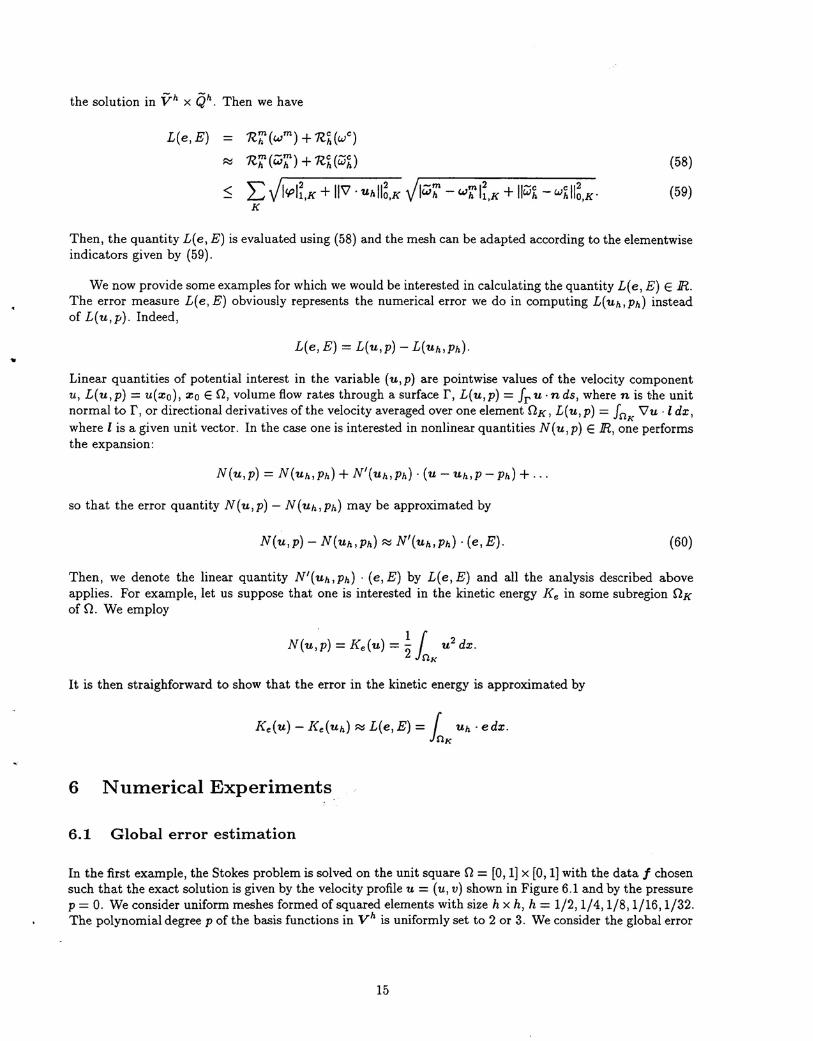
In the first example, the Stokes problem is solved on the unit square 0 = [0,1] x [0, 1] with the data 1chosensuch that the exact solution is given by the velocity profile u = (u, v) shown in Figure 6.1 and by the pressurep = O. We consider uniform meshes formed of squared elements with size h x h, h = 1/2,1/4,1/8,1/16,1/32.The polynomial degree P of the basis functions in Vh is uniformly set to 2 or 3. We consider the global error

15

Figure 6.1: Exact solution: (left) Velocity component u, (right) Velocity component v.

,

1/2 2 0.7620 0.5235 0.8520 0.85711/4 0.7300 0.8282 0.8983 0.90401/8 0.8154 0.9684 0.9797 0.98051/16 0.8184 0.9941 0.9947 0.9948

1/4 3 0.8406 0.8952 0.9679 0.96931/8 0.8815 0.9781 0.9895 0.9896

I h ~ .=(0,1) 1.:;:,0) 1.=(1,1) /I .=~:,1) I

Table 6.1: Normalized values of the approximations of IInf:II •.

estimator TJ defined as:

where t.p E V is approximated by a function t.ph E Vh or a function .,ph E Wh satisfying (24) or (34). Wecharacterize the extra degree (with respect to p) of the perturbations in Wh by the pair q = (qedge, qint),where q edge refers to the extra degree of the edge bubbles and q int to the extra degree of the interior bubbles.We recall that the cost of this error estimator is controlled by the cost in solving (24) or (34), that is, bythe size of Wh and the number of iterations performed using the Conjugate Gradient method. What issought is a trade-off between accuracy in the approximations.,ph and cost (time) spent to solve for them.Values of approximations of t.p and corresponding times are given in Tables 6.1- 6.2 for various values of h, pand q. The approximations are normalized with respect to overkills using q = (2,2) while the times arenormalized with respect to the times spent to solve for the solutions (Uh,Ph). The number of iterations inthe CG algorithm are determined according to a preset tolerance in solution accuracy.

We first observe that the performances greatly increases as the size of the problem increases. For example,the residual is estimated with a 99% accuracy while spending less than 7% of the solution time. We alsoobserve that it is approximated with less than one percent of error using Wh instead of Vh with q = (1,1).Moreover the number of iterations is kept very small while requiring reasonable accuracy of the order 10-2.

We also compute effectivity indices, defined as:

T}

,u,p = lI(e,E)11

16

,

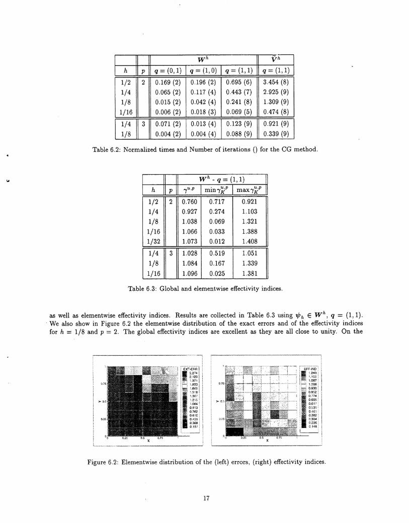
1/2 2 0.169 (2) 0.196 (2) 0.695 (6) 3.454 (8)1/4 0.065 (2) 0.117 (4) 0.443 (7) 2.925 (9)1/8 0.015 (2) 0.042 (4) 0.241 (8) 1.309 (9)1/16 0.006 (2) 0.018 (3) 0.069 (5) 0.474 (8)

1/4 3 0.071 (2) 0.013 (4) 0.123 (9) 0.921 (9)

1/8 0.004 (2) 0.004 (4) 0.088 (9) 0.339 (9)

I h 8 F (0,1) I q :;:,0) I q= (1,1)[J;@

Table 6.2: Normalized times and Number of iterations 0 for the CG method.

wh- q = (1,1)

h p /u,p min/~l max/'ll

1/2 2 0.760 0.717 0.9211/4 0.927 0.274 1.1031/8 1.038 0.069 1.3211/16 1.066 0.033 1.3881/32 1.073 0.012 1.408

1/4 3 1.028 0.519 1.0511/8 1.084 0.167 1.3391/16 1.096 0.025 1.381

Table 6.3: Global and elementwise effectivity indices .

as well as elementwise effectivity indices. Results are collected in Table 6.3 using 1/;h E Wh, q = (1,1).

. We also show in Figure 6.2 the element wise distribution of the exact errors and of the effectivity indicesfor h = 1/8 and p = 2. The global effectivity indices are excellent as they are all close to unity. On the

0..75

>c,s

0.:.25

:. £FF-1NO;

II ;·~~;l1:< 1.087:~ 1.008;!~I~;~', 0695'

i . 0.617'

i...., ,053"'.'.l;-;-:~~i: 0.304 j; 0.226 ~: C 14a:~

Figure 6.2: Elementwise distribution of the (left) errors, (right) effectivity indices.

17

other hand, the local effectivity indices, as it is expected for the case of a global error estimator, may behavepoorly, and in some cases drop to a value as low as 0.012. However, we observe that they are always nearunity in elements with large error, and diverge from unity only in elements with rather small error.

6.2 Backward facing step Stokes problem

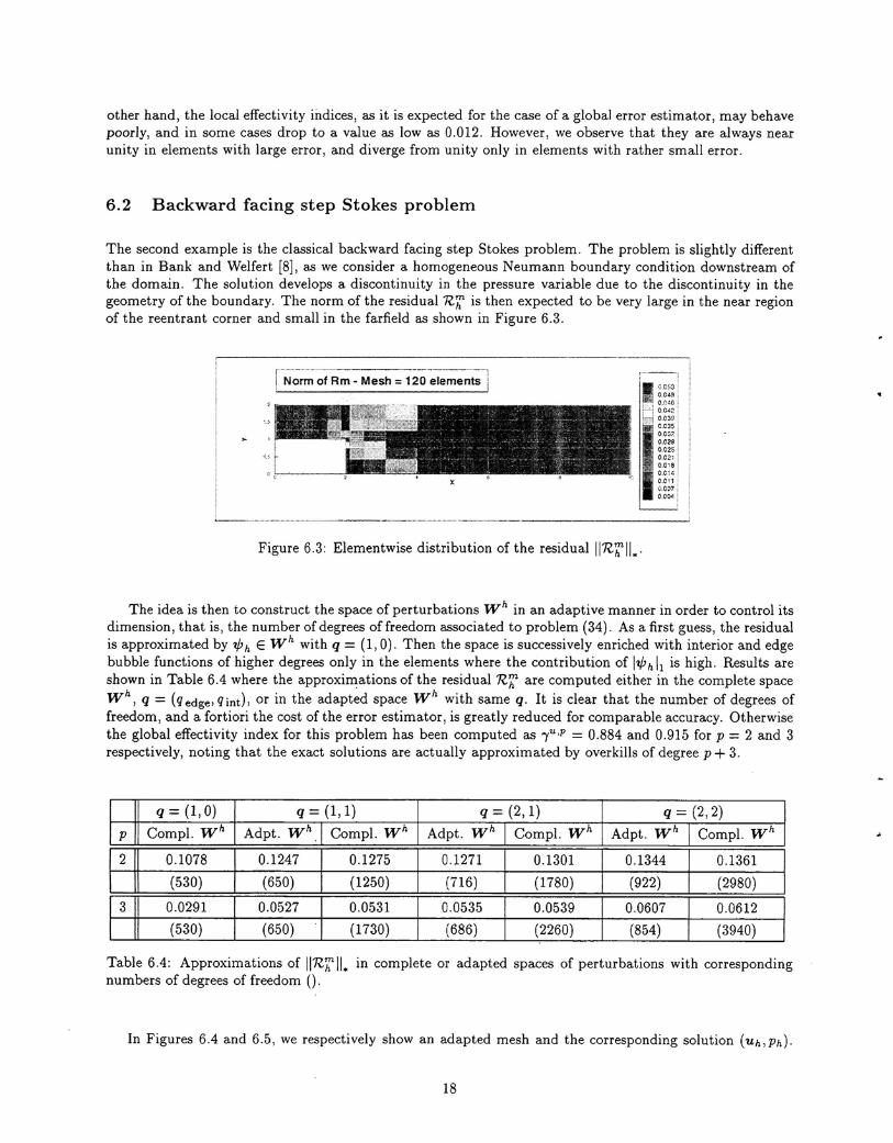
The second example is the classical backward facing step Stokes problem. The problem is slightly differentthan in Bank and Welfert [8], as we consider a homogeneous Neumann boundary condition downstream ofthe domain. The solution develops a discontinuity in the pressure variable due to the discontinuity in thegeometry of the boundary. The norm of the residual Rf: is then expected to be very large in the near regionof the reentrant corner and small in the farfield as shown in Figure 6.3.

, - - ..-. ··---·-·-----····-···1r Norm of Rm - Mesh = 120 elements i

Figure 6.3: Elementwise distribution of the residualllnf:II •.

The idea is then to construct the space of perturbations Wh in an adaptive manner in order to control itsdimension, that is, the number of degrees offreedom associated to problem (34). As a first guess, the residualis approximated by "ph E Wh with q = (1,0). Then the space is successively enriched with interior and edgebubble functions of higher degrees only in the elements where the contribution of l"ph 11 is high. Results areshown in Table 6.4 where the approximations of the residual nf: are computed either in the complete spaceWh, q = (qedge,qint), or in the adapted space Wh with same q. It is clear that the number of degrees offreedom, and a fortiori the cost of the error estimator, is greatly reduced for comparable accuracy. Otherwisethe global effectivity index for this problem has been computed as -ytl,p = 0.884 and 0.915 for p = 2 and 3respectively, noting that the exact solutions are actually approximated by overkills of degree p + 3.

q=(l,O) q = (1,1) q=(2,1) q = (2,2)p Compl. Wh Adpt. Wh Compl. Wh Adpt. Wh Compl. Wh Adpt. Wh Compl. Wh

2 0.1078 0.1247 0.1275 0.1271 0.1301 0.1344 0.1361(530) (650) (1250) (716) (1780) (922) (2980)

3 0.0291 0.0527 0.0531 0.0535 0.0539 0.0607 0.0612(530) (650) (1730) (686) (2260) (854) (3940)

Table 6.4: Approximations of IIRf:II. in complete or adapted spaces of perturbations with correspondingnumbers of degrees of freedom O.

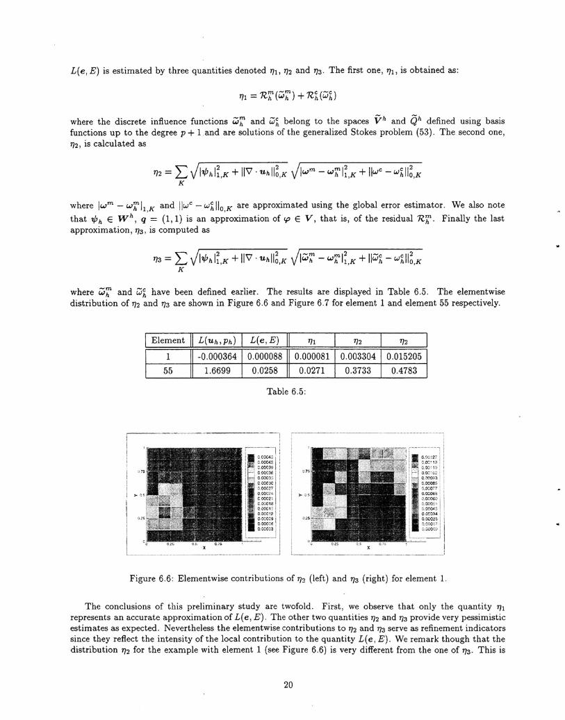
In Figures 6.4 and 6.5, we respectively show an adapted mesh and the corresponding solution (Uh,Ph).

18

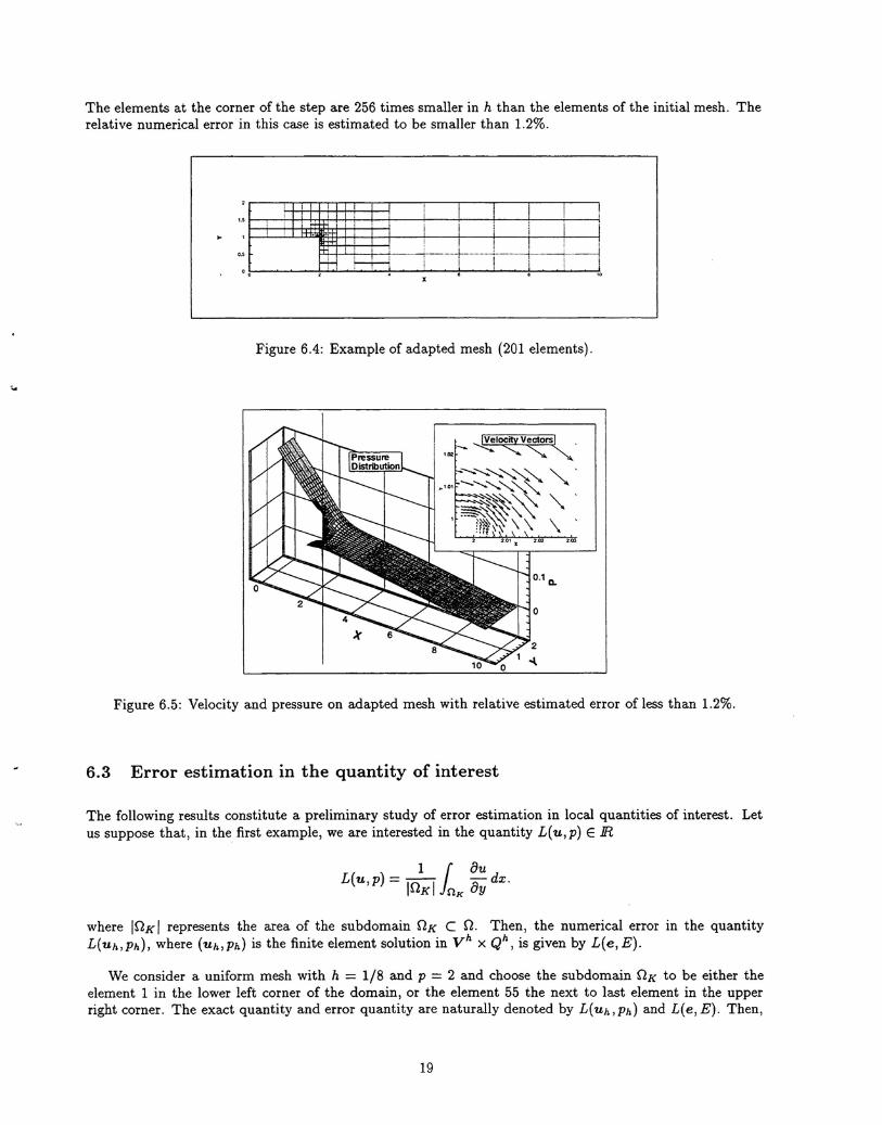
The elements at the corner of the step are 256 times smaller in h than the elements of the initial mesh. Therelative numerical error in this case is estimated to be smaller than 1.2%.

o.;

~ j

Figure 6.4: Example of adapted mesh (201 elements).

Figure 6.5: Velocity and pressure on adapted mesh with relative estimated error of less than 1.2%.

6.3 Error estimation in the quantity of interest

The following results constitute a preliminary study of error estimation in local quantities of interest. Letus suppose that, in the first example, we are interested in the quantity L( u, p) E IR

1 1 au-dx.L(u,p) = InKI n

Kay

where InK I represents the area of the subdomain nK C n. Then, the numerical error in the quantityL(uh,ph), where (Uh,Ph) is the finite element solution in Vh x Qh, is given by L(e,E).

We consider a uniform mesh with h = 1/8 and P = 2 and choose the subdomain nK to be either theelement 1 in the lower left corner of the domain, or the element 55 the next to last element in the upperright corner. The exact quantity and error quantity are naturally denoted by L( Uh ,Ph) and L( e, E). Then,

19

L(e, E) is estimated by three quantities denoted 1]1, 1]2 and 1]3. The first one, 1]1, is obtained as:

where the discrete influence functions w;;' and wh belong to the spaces Vh and Qh defined using basisfunctions up to the degree p + land are solutions of the generalized Stokes problem (53). The second one,1]2, is calculated as

1]2 =L VI1/7hli.K + 11\1· uhll~,K Vlwm- wf:li.K + IIwc

- w'i.II~.KK

where Iwm - wf:ll K and Ilwc - whllo K are approximated using the global error estimator. We also notethat 1/7hE Wh, q' = (1,1) is an ap~roximation of <p E V, that is, of the residual nf:. Finally the lastapproximation, 1]3, is computed as

1]3 = L VI1/7hli.K + 11\1· uhll~.K Vlw;;' - wf:I~.K + IP'i. - w'i.II~.KK

where w;;' and wI. have been defined earlier. The results are displayed in Table 6.5. The elementwisedistribution of 1]2 and 1]3 are shown in Figure 6.6 and Figure 6.7 for element 1 and element 55 respectively.

I Element ~ L(uh,Ph) I L(e,E) ~ 1]1 1]2 1]2

1 -0.000364 0.000088 0.000081 0.003304 0.015205

55 1.6699 0.0258 0.0271 0.3733 0.4783

Table 6.5:

:;.75

>- :..$

I 0.00:27

I,.~...,.~..j•.:••i.~i~..~.i. V.ocoes, .: v.XO..-7. . O.0i..'-06:'

.' 0.00060!:i.OCO::;!

.! 0.000<,, ! OCC(t.'l:4

iH)C02~J.r:OOF0.ocomi

Figure 6.6: Elementwise contributions of 1]2 (left) and 1]3 (right) for element 1.

The conclusions of this preliminary study are twofold. First, we observe that only the quantity 1]1

represents an accurate approximation of L( e, E). The other two quantities 1]2 and 1]3 provide very pessimisticestimates as expected. Nevertheless the elementwise contributions to 1]2 and 1]3 serve as refinement indicatorssince they reflect the intensity of the local contribution to the quantity L(e, E). We remark though that thedistribution 1]2 for the example with element 1 (see Figure 6.6) is very different from the one of 1]3. This is

20

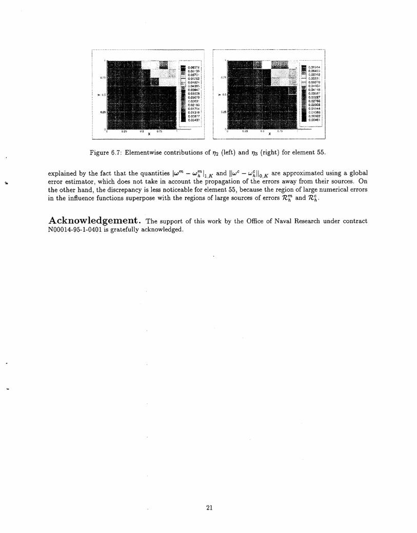
Figure 6.7: Elementwise contributions of 1]2 (left) and 1]3 (right) for element 55.

explained by the fact that the quantities Iwm - wf: 11K and IIwc - w~ 110K are approximated using a globalerror estimator, which does not take in account the propagation of the errors away from their sources. Onthe other hand, the discrepancy is less noticeable for element 55, because the region of large numerical errorsin the influence functions superpose with the regions of large sources of errors nf: and n'j..

Acknowledgement. The support of this work by the Office of Naval Research under contractN00014-95-1-0401 is gratefully acknowledged.

21

References

[1] M. AINSWORTH AND J. T. ODEN, A unified approach to a posteriori error estimation using elementresiduals methods, Numer. Math., 65 (1993), pp. 23-50.

[2] --:--, A posteriori error estimation in finite element analysis, Tech. Rep. 96-19, TICAM, The Universityof Texas at Austin, 1996. To Appear: Computational Advances. CMAME.

[3] I. BABUSKA AND W. RHEINBOLDT, A posteriori error estimates for the finite element method, Int. J.for Num. Meth. in Eng., 12 (1978), pp. 1597-1615.

[4] I. BABUSKA, T. STROUBOULIS, C. S. UPADHYAY, AND S. K. GANGARAJ, A posteriori estimation andadaptive control of the pollution error in the h-version of the finite element method, Int. J. for Num.Meth. in Eng., 38 (1995), pp. 4207-4235.

[5] R. E. BANK, Hierarchical bases and the finite element method. To Appear.

[6J R. E. BANK AND R. K. SMITH, A posteriori error estimates based on hierarchical bases, SIAM J.Numer. Anal., 30 (1993), pp. 921-935.

[7] R. E. BANK AND A. WEISER, Some a posteriori error estimates for elliptic partial differential equations,Math. Comp., 44 (1985), pp. 283-301.

[8] R. E. BANK AND B. D. WELFERT, A posteriori error estimates for the Stokes problem, SIAM J. Numer.AnaL, 28 (1991), pp. 591-623.

[9] R. BECKER AND R. RANNACHER, A feedback approach to error control in finite elements methods: Basicanalysis and examples, Preprint 96-52, Institut fur Angewandte Mathematik, Universitat Heidelberg,(1996).

[10] -, Weighted a posteriori error control in FE method, in ENUMATH-95, Paris, Sept. 1995.

[11] L. DEMKOWICZ, J. T. ODEN, AND T. STROUBOULIS, Adaptive finite elements for flow problems withmoving boundaries. Part 1: Variational principles and a posteriori error estimates, Compo Meth. inAppl. Mech. and Eng., 46 (1984), pp. 217-251.

[12] V. GIRAULT AND P.-A. RAVIART, Finite Element Methods for Navier-Stokes Equations, Springer-Verlag, 1986.

[13] P. LADEVEZE AND D. LEGUlLLON, Error estimate procedure in the finite element method and applica-tions, SIAM J. Numer. Anal., 20 (1983), pp. 485-509.

[14] J. T. ODEN, L. DEMKOWlCZ, W. RACHOWICZ, AND O. HARDY, Toward a universal h-p adaptivefinite element strategy. Part 1: Constrained approximation and data structure, Compo Meth. in Appl.Mech. and Eng., 77 (1989), pp. 113-180.

[15] J. T. ODEN AND Y. FENG, Local and pollution error estimation for finite element approximations ofelliptic boundary value problems, J. Comput. Appl. Math., 74 (1996), pp. 245-293.

[16] J. T. ODEN, W. Wu, AND M. AINSWORTH, An a posteriori error estimate for finite element approxi-mations of the Navier-Stokes equations, Compo Meth. in Appl. Mech. and Eng., III (1993), pp. 185-202.

[17] B. SZABO AND I. BABUSKA, Finite Element Analysis, John Wiley and Sons, 1991.

[18] R. VERFURTH, A posteriori error estimators for the Stokes equations, Numer. Math., 55 (1989), pp. 309-325. .

[19] R. VERFURTH, A Review of A posteriori Error Estimation and Adaptive Mesh-refinement Techniques,Wiley-Teubner, 1996.

22