Lipschitz equivalence of self-similar sets and hyperbolic ...archive.ymsc.tsinghua.edu.cn/pacm_download/221/8454-Lipschitz... · Lipschitz equivalence of self-similar sets and hyperbolic

Available online at www.sciencedirect.com

Advances in Mathematics 235 (2013) 555–579www.elsevier.com/locate/aim

Lipschitz equivalence of self-similar sets and hyperbolicboundaries

Jun Jason Luoa,b,∗, Ka-Sing Laua

a Department of Mathematics, The Chinese University of Hong Kong, Hong Kongb Department of Mathematics, Shantou University, Shantou, Guangdong 515063, PR China

Received 14 May 2012; accepted 17 December 2012

Communicated by Kenneth Falconer

Abstract

Kaimanovich (2003) [9] introduced the concept of augmented tree on the symbolic space of a self-similar set. It is hyperbolic in the sense of Gromov, and it was shown by Lau and Wang (2009) [12] thatunder the open set condition, a self-similar set can be identified with the hyperbolic boundary of the tree. Inthe paper, we investigate in detail a class of simple augmented trees and the Lipschitz equivalence of suchtrees. The main purpose is to use this to study the Lipschitz equivalence problem of the totally disconnectedself-similar sets which has been undergoing some extensive development recently.c⃝ 2012 Elsevier Inc. All rights reserved.

Keywords: Augmented tree; Hyperbolic boundary; Incidence matrix; Lipschitz equivalence; OSC; Primitive;Rearrangeable; Self-similar set; Self-affine set

1. Introduction

Two compact metric spaces (X, dX ) and (Y, dY ) are said to be Lipschitz equivalent, and denoteby X ≃ Y , if there is a bi-Lipschitz map σ from X onto Y , i.e., σ is a bijection and there is aconstant C > 0 such that

C−1dX (x, y) ≤ dY (σ (x), σ (y)) ≤ CdX (x, y) ∀ x, y ∈ X.

∗ Corresponding author at: Department of Mathematics, The Chinese University of Hong Kong, Hong Kong.E-mail addresses: [email protected] (J.J. Luo), [email protected] (K.-S. Lau).

0001-8708/$ - see front matter c⃝ 2012 Elsevier Inc. All rights reserved.doi:10.1016/j.aim.2012.12.010

http://www.elsevier.com/locate/aim

http://dx.doi.org/10.1016/j.aim.2012.12.010

http://www.elsevier.com/locate/aim

mailto:[email protected]

mailto:[email protected]

http://dx.doi.org/10.1016/j.aim.2012.12.010

556 J.J. Luo, K.-S. Lau / Advances in Mathematics 235 (2013) 555–579

It is easy to see that if X ≃ Y , then dimH X = dimH Y = s, where dimH denotes the Haus-dorff dimension. A more intensive study of this was due to Cooper and Pignartaro [2] in the late80s, they showed that for certain Cantor sets X, Y on R, the Lipschitz equivalence implies thatthere exists a bi-Lipschitz map σ and a λ > 0 such that Hs(σ (E)) = λHs(E). In another con-sideration, Falconer and Marsh [5] proved that for quasi-self-similar circles, they are Lipschitzequivalent if and only if they have the same Hausdorff dimension.

The recent interest of the Lipschitz equivalence is due to the path breaking study of Rao,Ruan and Xi [18] on a question of David and Semmes [3] on certain special self-similar set onR to be dust-like (see Example 5.2). They observed a graph directed relationship in the under-lying iterated function system (IFS), and made use of this to construct the needed bi-Lipschitzmap. There is a number of generalizations on R and Rd for the totally disconnected self-similarsets with uniform contraction ratio or with logarithmically commensurable contraction ratios([4,19,23–25]). For certain Cantor-type sets on Rd with non-equal contraction ratios, Rao, Ruanand Wang [17] had an elegant algebraic criterion for them to be Lipschitz equivalent, which im-proved a condition of Falconer and Marsh in [6]. Other considerations can be found in [15,16,22].

So far the investigation of the Lipschitz equivalence is very much restricted on a few specialself-similar sets. In this paper, we will provide a broader framework to study the problem throughthe concept of augmented (rooted) tree. For an IFS Si

mi=1 of contractive similitudes on Rd

(assume equal contraction ratio in the present situation) and the associated self-similar set K , weuse X =

∞

n=0 Σ n , Σ = 1, . . . , m to denote the symbolic space. Then X has a natural graphstructure, and we denote the edge set by Ev (v for vertical). We define a horizontal edge for a pair(u, v) in X × X if u, v ∈ Σ n and Su(K ) ∩ Sv(K ) = ∅, and denote this set of edges by Eh . Theaugmented tree is defined as the graph (X, E ) where E = Ev ∪ Eh .

Such augmented tree was first introduced by Kaimanovich [9] on the Sierpinski gasket inorder to incorporate the intersection of the cells to the symbolic space, and was developed byLau and Wang [12] to general self-similar sets. It was proved that if an IFS satisfies the open setcondition (OSC), then the augmented tree is hyperbolic in the sense of Gromov. There is a hyper-bolic metric ρ on X , which induces a hyperbolic boundary (∂ X, ρ). The hyperbolic boundary isshown to be homeomorphic to K ; moreover under certain mild condition, the homeomorphismis actually a Holder equivalent map. This setup is used to study the random walks on (X, E ) andtheir Martin boundaries [13].

Based on this, our approach to the Lipschitz equivalence of the self-similar sets is to lift theconsideration to the augmented trees (X, E ). We define a horizontal connected component of Xto be the maximal connected horizontal subgraph T in some level Σ n . Let C be the set of allhorizontal connected components of X . For T ∈ C , we use TΣ to denote the set of offspringsof T , and consider T ∪ TΣ as a subgraph in X . We say that T, T ′

∈ C are equivalent if theyare graph isomorphic. We call X simple if there are finitely many equivalence classes. Under thiscondition, we can define an incidence matrix

A = [ai j ]

for the equivalence classes as follows: choose any component T belonging to the class Ti , andlet Zi1, . . . , Ziℓ be the connected components of the descendants of T . The entry ai j denotes thenumber of Zik that belonging to the class T j .

It is shown that a simple augmented tree X is always hyperbolic, and the relationship of thehyperbolic boundary and the self-similar set is analogous to the case with OSC (Propositions 3.4and 3.5). Our basic theorem, to put it into a simple statement, is (assuming the IFS has equalcontraction ratio):

J.J. Luo, K.-S. Lau / Advances in Mathematics 235 (2013) 555–579 557

Theorem 1.1. Suppose the augmented tree (X, E ) is simple and the corresponding incidencematrix A is primitive (i.e., An > 0 for some n > 0), then ∂(X, E ) ≃ ∂(X, Ev).

We call a self-similar set K dust-like if it satisfies Si (K ) ∩ S j (K ) = ∅ for i = j . By reducingthe Lipschitz equivalence on the trees in Theorem 1.1 to the self-similar sets (Proposition 3.5,Theorem 3.10), we have

Theorem 1.2. (i) If in addition to the condition in Theorem 1.1, the IFS satisfies some mildcondition (H) (see Section 2), then K is Lipschitz equivalent to a dust-like self-similar set.

(ii) If K and K ′ are as in (i) and the two IFS’s have the same number of similitudes and thesame contraction ratio, then they are Lipschitz equivalent.

The proof of Theorem 1.1 depends on constructing a near-isometry between the augmentedtree (X, E ) and (X, Ev). The crux of the construction is to use a technique of rearrangement ofedges (Section 4), which is based on an idea of Deng and He in [4]. Actually we prove a lessrestrictive form of Theorem 1.1 (Theorem 3.7) in terms of rearrangeable matrices. Theorem 1.1follows from another theorem (Theorem 3.8) that the primitive property implies rearrangability.

We will provide an easy way to check an augmented tree being simple (Lemma 5.1), whichis more efficient to apply to various examples than the graph directed systems that were usedin the previous studies [4,18,24]. Theorem 1.2 essentially covers all the known cases so far, italso covers some new classes of IFS’s that have overlaps and rotations (see Section 5). Moreoverthe theory can be extended from the self-similar IFS to the self-affine IFS: it is easy to see thatthe notion of augmented tree and the results on such tree remain unchanged. For self-affine setson Rd , we can still establish the Lipschitz equivalence, making use of a device in [8] which re-places the Euclidean distance by an ultra-metric adapted to the underlying self-affine system (seeTheorem 3.14).

The paper is organized as follows. In Section 2, we recall some well-known results on hy-perbolic graphs and set up the augmented tree. In Section 3, we introduce the notion of simpleaugmented tree, and derive its basic properties. Theorem 1.1 is stated there, and Theorem 1.2 to-gether with other consequences is proved. The proof of Theorem 1.1 and the involved concept ofrearrangement are given in Section 4. In Section 5, we provide several new examples to illustrateour results; some concluding remarks and open questions are given in Section 6.

2. Preliminaries

Let X be a countably infinite set, we say that X is a graph if it is associated with a symmetricsubset E of (X × X) \ (x, x) : x ∈ X; we call x ∈ X a vertex, (x, y) ∈ E an edge, whichis more conveniently denoted by x ∼ y (intuitively, x, y are neighborhoods to each other). By apath in X from x to y, we mean a finite sequence x = x0, x1, . . . , xn = y such that xi ∼ xi+1,

i = 0, . . . , n − 1. We always assume that the graph X is connected, i.e., there is a path joiningany two vertices x, y ∈ X . We call X a tree if the path between any two points is unique. Weequip a graph X with an integer-valued metric d(x, y), which is the minimum among the lengthsof the paths from x to y; the corresponding geodesic path is denoted by π(x, y) and its length by|π(x, y)|(=d(x, y)). Let o ∈ X be a fixed point in X and call it the root of the graph. We use |x |

to denote d(o, x), and say that x belongs to the n-th level of the graph if d(o, x) = n.The notion of hyperbolic graph was introduced by Gromov [7,21]. First we define the Gromov

product of any two points x, y ∈ X by

|x ∧ y| =12(|x | + |y| − d(x, y)).


We say that X is hyperbolic (with respect to o) if there is δ > 0 such that

|x ∧ y| ≥ min|x ∧ z|, |z ∧ y| − δ ∀ x, y, z ∈ X.

Note that this is equivalent to a more geometric characterization: there exists a δ′ such that forany three points in X , the geodesic triangle is δ′-thin: any point on one side of the triangle hasdistance less than δ′ to some point on one of the other two sides.

For a fixed a > 0 with a′= exp(δa) − 1 <

√2 − 1, we define an ultra-metric ρa(·, ·) on X

by

ρa(x, y) =

exp(−a|x ∧ y|) if x = y,

0 otherwise.(2.1)

Then

ρa(x, y) ≤ (1 + a′) maxρa(x, z), ρa(z, y) ∀ x, y, z ∈ X,

which is equivalent to the path metric

θa(x, y) = inf

n

i=1

ρa(xi−1, xi ) : n ≥ 1, x = x0, x1, . . . , xn = y, xi ∈ X

.

Since θa and ρa determine the same topology as long as a′ <√

2 − 1, we will use ρa to replaceθa for simplicity.

Definition 2.1. The hyperbolic boundary of X is defined as ∂ X = X \ X where X is the com-pletion of X under ρa .

The metric ρa can be extended onto ∂ X , and under which ∂ X is a compact set. It is oftenuseful to identify ξ ∈ ∂ X with a geodesic ray in X that converge to ξ , i.e., an infinite path π [x1,

x2, . . .] such that xi ∼ xi+1 and any finite segment of the path is a geodesic. It is knownthat two geodesic rays π [x1, x2, . . .], π[y1, y2, . . .] represent the same ξ ∈ ∂ X if and only if|xn ∧ yn| → ∞ as n → ∞.

Our interest is on the following tree structure introduced by Kaimanovich which is used tostudy the self-similar sets ([9,12]). For a tree X with a root o, we use Ev to denote the set ofedges (v for vertical). We introduce additional edges on each level x : d(o, x) = n, n ∈ Nas follows. Let x−k denote the k-th ancestor of x , the unique point in the (n − k)-th level that isjoined by a unique path.

Definition 2.2. Let X be a tree with a root o. Let Eh ⊂ (X × X) \ (x, x) : x ∈ X such that itis symmetric and satisfies:

(x, y) ∈ Eh ⇒ |x | = |y| and either x−1= y−1 or (x−1, y−1) ∈ Eh .

We call elements in Eh horizontal edges, and for E = Ev ∪ Eh , (X, E ) is called an augmentedtree.

Following [12], we say that a path π(x, y) is a horizontal geodesic if it is a geodesic and itconsists of horizontal edges only. It is called a canonical geodesic if there exist u, v ∈ π(x, y)

such that:(i) π(x, y) = π(x, u) ∪ π(u, v) ∪ π(v, y) with π(u, v) a horizontal path and π(x, u), π(v, y)

vertical paths;(ii) for any geodesic path π ′(x, y), dist(o, π(x, y)) ≤ dist(o, π ′(x, y)).


Note that condition (ii) is to require the horizontal part of the canonical geodesic to be on thehighest level. The following basic theorem was proved in [12]:

Theorem 2.3. Let X be an augmented tree. Then(i) Let π(x, y) be a canonical geodesic, then |x ∧ y| = l − h/2, where l and h are the level

and the length of the horizontal part of the geodesic.(ii) X is hyperbolic if and only if there exists a constant k > 0 such that any horizontal part

of a geodesic is bounded by k.

The premier application of the augmented trees is to use their hyperbolic boundaries to studythe self-similar sets. Throughout the paper, we assume a self-similar set K is generated by aniterated function system (IFS) Si

mi=1 on Rd where

Si (x) = r Ri x + di , i = 1, . . . , m (2.2)

with 0 < r < 1, Ri is an orthogonal matrix, and di ∈ Rd . It is well-known that K satisfies K =mi=1 Si (K ). Let Σ = 1, . . . , m and let X =

∞

n=0 Σ n be the symbolic space representing theIFS (by convention, Σ 0

= ∅, and we still denote it by o). For u = i1 · · · in , we use Su to denotethe composition Si1 · · · Sin .

Let Ev be the set of vertical edges corresponding to the nature tree structure on X with o as aroot. In [12], a set of horizontal edges Eh is defined as

Eh = (u, v) : |u| = |v|, u = v and Ku ∩ Kv = ∅ ,

where Ku = Su(K ). Let E = Ev ∪ Eh , then (X, E ) is an augmented tree induced by the self-similar set.

If the IFS is strongly separated (i.e., Si (K )∩ S j (K ) = ∅ for i = j), then K is called dust-like.It is clear that in this case, Eh = ∅, and ρa coincides with the natural metric on the symbolicspace:

ϱ(x, y) = exp(−a maxk : xi = yi , i ≤ k).

In [12], it was proved that under the open set condition (OSC), Theorem 2.3(ii) implies that theabove augmented tree is hyperbolic, and the nature map Φ : ∂ X → K is a homeomorphism.Moreover if in addition, the IFS satisfiescondition (H): there exists a constant c > 0 such that for any integer n ≥ 1 and words u, v ∈ Σ n ,

Ku ∩ Kv = ∅ ⇒ dist(Ku, Kv) ≥ crn . (2.3)

Then for α = − log r/a, Φ satisfies the following Holder equivalent property:

C−1|Φ(ξ) − Φ(η)| ≤ ρa(ξ, η)α ≤ C |Φ(ξ) − Φ(η)| ∀ ξ, η ∈ ∂ X.

Condition (H) is satisfied by the standard self-similar sets, for example, the generating IFS hasthe OSC and all the parameters of the similitudes are integers. However there are also examplesthat condition (H) is not satisfied (see [12] for an example such that the similitudes involveirrational translations).

From Definition 2.2, we see that the choice of the horizontal edges for the augmented treecan be quite flexible, for example we can use Ku ∩ Kv to have positive dimension to define Eh .In this paper, we will use another setting by replacing K with a bounded closed invariant set J(i.e., Si (J ) ⊂ J for each i), namely

Eh = (u, v) : |u| = |v|, u = v and Ju ∩ Jv = ∅ . (2.4)


We can take J = K as before or in many situations, take J = U for the U in the OSC (seethe examples in Section 5). The above statements on the hyperbolicity of the augmented treeand the homeomorphism of the boundary still valid by adopting the same proof; for the Holderequivalence, we use the following modification of condition (H) for J , which will be used againin proving Proposition 3.5.

Lemma 2.4. Suppose the IFS in (2.2) satisfies condition (H), then for any bounded closedinvariant set J , there exists c′ > 0 and k ≥ 0 such that for any n ≥ 0 and u, v ∈ Σ n ,

Ju ∩ Jv = ∅ ⇒ dist(Jui, Jvj) ≥ c′rn∀ i, j ∈ Σ k .

Proof. Let c be the constant in the definition of condition (H). For the bounded closed invariantset J , we have K ⊆ J and the Hausdorff distance dH (Ki, Ji) ≤ c1rk for all i ∈ Σ k . In particularwe choose k such that c1rk < c/3.

Now if u, v ∈ Σ n, Ju ∩ Jv = ∅, then Ku ∩ Kv = ∅, it follows from condition (H) thatdist(Ku, Kv) ≥ crn for u, v ∈ Σ n . Applying this and the above to n + k, we have

dist(Jui, Jvj) ≥ dist(Kui, Kvj) − dH (Kui, Jui) − dH (Kvj, Jvj)

≥ crn− (2c/3) rn

≥ (c/3)rn∀ i, j ∈ Σ k .

The lemma follows by taking c′= c/3.

We remark that the augmented tree (X, E ) depends on the choice of the bounded invariant setJ . But under the OSC, the hyperbolic boundary is the same as they can be identified with theunderlying self-similar set.

We conclude this section with the following simple relationship of the totally disconnectedself-similar set and the structure of the augmented tree. The more explicit study of their Lipschitzequivalence will be carried out in detail in the rest of the paper. By a horizontal connectedcomponent of an augmented tree, we mean a maximal connected horizontal subgraph on somelevel Σ n of X .

Proposition 2.5. Suppose the cardinality of any horizontal component in the augmented treeinduced by the IFS in (2.2) is uniformly bounded, then the associated self-similar set K is totallydisconnected.

The converse is also true if the about IFS is on R1 and satisfies the OSC.

Proof. Suppose K is not totally disconnected, then there is a connected component C ⊂ Kcontains more that one point. Note that for any n > 0, K =

i∈Σ n Ki. Let Ki1 ∩ C = ∅. If

C \ Ki1 = ∅, then it is a relatively open set in C , and as C is connected,

∂C (C \ Ki1) ∩ ∂C (Ki1 ∩ C) = ∅.

(∂C (E) means the relative boundary of E in C). Let x be in the intersection, there exists i2 ∈ Σ n

such that x ∈ Ki1 ∩ Ki2 and Ki2 ∩ (C \ Ki1) = ∅.Inductively, if

kj=1 Ki j does not cover C , then we can repeat the same procedure to find

ik+1 ∈ Σ n such that

Kik+1 ∩

k

j=1

Ki j

= ∅ and Kik+1 ∩

C \

kj=1

Ki j

= ∅.


Since K =

i∈Σ n Ki, this process must end at some step, say ℓ, and in this case C ⊂ℓ

j=1 Ki j .Since the diameter |Ki j | = rn

|K | → 0 as n → ∞, ℓ must tend to infinity, which contradicts theuniform boundedness of the horizontal connected components Σ n .

For the converse, we assume that the IFS is defined on R. Note that if K ⊂ R is totally dis-connected, then dimH K = s < 1 [20]. Let µ denote the restriction of the s-Hausdorff measureon K . Without loss of generality, we assume µ(K ) = 1. Then it is well-known that for any pointx ∈ K and any 0 < t < |K | (where |K | denotes the diameter of K ),

C1 <µ(B(x, t))

t s < C2,

where C1, C2 are constants independent of x and t .Suppose i1, i2, . . . , ik is a finite sequence of distinct words in Σ n and is in a horizontal con-

nected component (we take J = K for convenience), i.e., Ki j ∩ Ki j+1 = ∅ for 1 ≤ j ≤ k − 1.Let G be the smallest interval containing Ki1 , . . . , Kik . Let x ∈ G ∩ K , and let t = |G|. Thenthe Hausdorff measure µ implies

µ(B(x, t)) ≥ krns .

This together with t = |G| ≤ krn|K | implies

k1−s

|K |s=

krns

(krn|K |)s ≤µ(B(x, t))

t s ≤ C2.

Hence k is uniformly bounded.

3. Lipschitz equivalence and the main theorems

In this rest of the paper, unless otherwise stated, we will assume the augmented tree (X, E )

is associated with the symbolic space of the IFS Si mi=1 in (2.2), and E = Eh ∪ Ev where Eh is

defined by a fixed bounded closed invariant set J as in (2.4). We introduce a class of mappingsbetween two hyperbolic graphs which plays a key role in the Lipschitz equivalence.

Definition 3.1. Let X and Y be two hyperbolic graphs and let σ : X → Y be a bijective map.We say that σ is a near-isometry if there exists c > 0 such that|π(σ(x), σ (y))| − |π(x, y)|

≤ c ∀ x, y ∈ X.

Remark. By checking π(o, x), it is easy to show that the above definition implies|σ(x)| −

|x | ≤ c +3|σ(o)|+ k where k is the bound of the horizontal geodesic in Theorem 2.3(ii). Hence

the above definition is equivalent to|σ(x)| − |x | < c,

|π(σ(x), σ (y))| − |π(x, y)| ≤ c ∀ x, y ∈ X

(with different constant c).

Proposition 3.2. Let X, Y be two hyperbolic augmented trees that are equipped with the hyper-bolic metrics with the same parameter a (as in (2.1)). Suppose there exists a near-isometry σ :

X → Y , then ∂ X ≃ ∂Y .

Proof. With the notation as in Theorem 2.3(i), it follows that for x = y ∈ X ,

|π(x, y)| = |x | + |y| − 2l + h, |π(σ(x), σ (y))| = |σ(x)| + |σ(y)| − 2l ′ + h′.


From the definition of σ (and the remark), we have|σ(x)| − |x |, |σ(y)| − |y|

≤ c, |l − l ′| ≤ 3c/2 + k/2, and |h − h′| ≤ k

for some k > 0 (where k is the hyperbolic constant as in Theorem 2.3(ii)). By Theorem 2.3(i),

|x ∧ y| = l − h/2 and |σ(x) ∧ σ(y)| = l ′ − h′/2.

It follows that|σ(x) ∧ σ(y)| − |x ∧ y| = |l ′ − h′/2 − l + h/2| ≤ 3c/2 + k := k′.

Let λ = eak′

, together with the definition of the ultra-metric ρa(x, y) = exp(−a|x ∧ y|) in (2.1),we conclude that

λ−1ρa(x, y) ≤ ρa(σ (x), σ (y)) ≤ λρa(x, y) ∀ x, y ∈ X.

By extending the metrics to the boundaries ∂ X, ∂Y , the above implies σ is a bi-Lipschitz mapfrom ∂ X onto ∂Y .

Let C be the set of all horizontal connected components of X . For T ∈ C , we let TΣ = ui :

u ∈ T, i ∈ Σ be the set of offsprings of T . Note that if two distinct components T, T ′∈ C lie

in the same level, then TΣ is not connected to T ′Σ , equivalently, i∈TΣ

Ji

∩

j∈T ′Σ

Jj

= ∅. (3.1)

This follows easily from Sui (J )∩ Sv j (J ) ⊂ Su(J )∩ Sv(J ) = ∅ for all u ∈ T, v ∈ T ′, i, j ∈ Σ .By regarding T ∪ TΣ as a subgraph in X . We say that T, T ′

∈ C are equivalent, denoted byT ∼ T ′, if there exists a graph isomorphism

g : T ∪ TΣ → T ′∪ T ′Σ ,

that is, g is a bijection such that g and g−1 preserve the vertical and horizontal edges. It is easyto check that ∼ is indeed an equivalence relation. We use [T ] to denote the equivalence class andcall it a connected class determined by T . Obviously, o is the connected class determined bythe root o.

Definition 3.3. An augmented tree X is called simple (with respect to the defining boundedclosed invariant set J ) if there are finitely many connected classes, i.e., C / ∼ is finite.

Proposition 3.4. A simple augmented tree is always hyperbolic.

Proof. Note that for each geodesic π(x, y) in X , the horizontal part must be contained in a hori-zontal component of the augmented tree. Since there are finitely many connected classes [T ], andeach T contains finitely many vertices, it follows that the horizontal part of π(x, y) is uniformlybounded, and hence hyperbolic by Theorem 2.3(ii).

In the following we show that the hyperbolic boundary of a simple augmented tree is Holderequivalent to the self-similar set, which is similar to the case in [12] for the OSC.

Proposition 3.5. Let Si mi=1 be an IFS satisfies condition (H) in (2.3), and assume that the

corresponding augmented tree (X, E ) is simple. Then there exists a bijection Φ : ∂ X → K


satisfying the Holder equivalent property:

C−1|Φ(ξ) − Φ(η)| ≤ ρa(ξ, η)α ≤ C |Φ(ξ) − Φ(η)|, (3.2)

where α = − log r/a and C > 0 is a constant.

Proof. The proof is essentially the same as in [12] by replacing K with the invariant set J in Eh .We sketch the main idea of proof here. For any geodesic ray ξ = π [u1, u2, . . .], we define

Φ(ξ) = limn→∞

Sun (x0)

for some x0 ∈ J . Then the mapping is well-defined and is a bijection (see Lemma 4.1, Theorem4.3 in [12]).

To show that Φ satisfies (3.2), let ξ = π [u0, u1, u2, . . .], η = π [v0, v1, v2, . . .] be anytwo non-equivalent geodesic rays in X . Then there is a canonical bilateral geodesic γ joining ξ

and η:

γ = π [. . . , un+1, un, t1, . . . , tℓ, vn, vn+1, . . .]

with un, t1, . . . , tℓ, vn ∈ Σ n . It follows that

|Sun (x0) − Svn (x0)| ≤ (ℓ + 2)rn|J |.

Since X is simple, ℓ is uniformly bounded (by Proposition 3.4). Note that Φ(ξ) ∈ Juk and Φ(η)

∈ Jvk for all k ≥ 0, hence

|Φ(ξ) − Sun (x0)|, |Φ(η) − Svn (x0)| ≤ rn|J |.

Therefore

|Φ(ξ) − Φ(η)| ≤ |Φ(ξ) − Sun (x0)| + |Sun (x0) − Svn (x0)| + |Φ(η) − Svn (x0)|

≤ C1rn .

Since γ is a bilateral canonical geodesic, we have |ξ ∧ η| = n − (ℓ + 1)/2 and ℓ is uniformlybounded. By using ρa(ξ, η) = exp(−a|ξ ∧ η|), we see that

|Φ(ξ) − Φ(η)| ≤ Cρa(ξ, η)α.

On the other hand, assume that ξ = η. Since γ is a geodesic, it follows that (un+1, vn+1) ∈ Eh ,and hence Jun+1 ∩ Jvn+1 = ∅. By Lemma 2.4, there is k (independent of n) such that

Ju ∩ Jv = ∅ ⇒ dist(Jui, Jvj) ≥ c′rn∀ i, j ∈ Σ k .

Referring to γ = π [. . . , un+1, un, t1, . . . , tℓ, vn, vn+1, . . .], we have Φ(ξ) ∈ Jun+k+1 , Φ(ξ) ∈

Jvn+k+1 . It follows that

|Φ(ξ) − Φ(η)| ≥ dist(Jun+k+1 , Jvn+k+1) ≥ c′rn,

and |Φ(ξ) − Φ(η)| ≥ c′′ρa(ξ, η)α follows by the definition of ρa as the above.

For a simple augmented tree X , we label the connected classes as T1, . . . ,Tr and introducean r × r incidence matrix

A = [ai j ]r×r (3.3)


for the connected classes. The entries ai j are defined as follows. For any 1 ≤ i ≤ r , take ahorizontal connected component T in X such that [T ] = Ti . Let Zi1, . . . , Ziℓ be the horizontalconnected components consisting of offsprings generated by T , i.e., TΣ =

ℓk=1 Zik , and define

ai j = #k : 1 ≤ k ≤ ℓ, [Zik] = T j .

Observe that ai j is independent of the choice of the components in the equivalence classes. It isclear that for T, T ′

∈ C , [T ] = [T ′] implies #T = #T ′. But the converse is not true. As a direct

consequence of the definition, we have

Proposition 3.6. Let b = [b1, . . . , br ]t where bi = #T where [T ] = Ti , then Ab = mb.

The following theorem is for Lipschitz equivalence on the hyperbolic boundaries, it is thecrucial step to establish the equivalence for the self-similar sets.

Theorem 3.7. Suppose the augmented tree (X, E ) is simple, and suppose the corresponding in-cidence matrix A is (m, b)-rearrangeable (where the m and b are defined as in Proposition 3.6).Then there is a near-isometry between (X, E ) and (X, Ev), so that ∂(X, E ) ≃ ∂(X, Ev).

The notion of rearrangeable matrix is an important tool to construct the near-isometry. Sincethe concept is a little complicated, we will introduce this in more detail, and prove Theorem 3.7together with the following theorem in the next section.

Theorem 3.8. If the incidence matrix A is primitive, then Ak is (mk, b)-rearrangeable for somek > 0. Consequently ∂(X, E ) ≃ ∂(X, Ev).

As a direct consequence, we have

Corollary 3.9. Under the assumption on Theorem 3.7 (or Theorem 3.8), then (∂(X, E ), ρa) istotally disconnected.

By Theorem 3.7 we obtain the following Lipschitz equivalence on the self-similar sets.

Theorem 3.10. Let K and K ′ be self-similar sets that are generated by two IFS’s as in (2.2) withthe same number of similitudes and the same contraction ratio, and satisfy condition (H) in (2.3).Assume the associated augmented trees are simple and the incidence matrices are (m, b)-rearrangeable (in particular, primitive). Then K and K ′ are Lipschitz equivalent, and are alsoLipschitz equivalent to a dust-like self-similar set.

Proof. It follows from Theorem 3.7 that

∂(X, E ) ≃ ∂(X, Ev) = ∂(Y, Ev) ≃ ∂(Y, E ) (3.4)

(for the respective metrics ρa). Let ϕ : ∂(X, E ) → ∂(Y, E ) be the bi-Lipschitz map. With noconfusion, we just denote these two boundaries by ∂ X , ∂Y as before.

By Proposition 3.5, there exist two bijections Φ1 : ∂ X → K and Φ2 : ∂Y → K ′ satisfying(3.2) with constants C1, C2, respectively. Define τ : K → K ′ as

τ = Φ2 ϕ Φ−11 .

Then

|τ(x) − τ(y)| ≤ C2 ρa(ϕ Φ−11 (x), ϕ Φ−1

1 (y))α

≤ C2Cα0 ρa(Φ−1

1 (x),Φ−11 (y))α

≤ C2Cα0 C1 |x − y|.


Let C ′= C2Cα

0 C1, then

|τ(x) − τ(y)| ≤ C ′|x − y|.

Similarly, we have C ′−1|x − y| ≤ |τ(x) − τ(y)|. Therefore τ : K → K ′ is a bi-Lipschitz map.

For the last statement, we can regard (X, Ev) as the augmented tree of an IFS that is stronglyseparated, and then apply the above conclusion.

Corollary 3.11. The IFS in Theorem 3.10 satisfies the OSC.

Proof. We make use of the following well-known result of Schief [20] on a self-similar set K : lets be the similarity dimension of K , then the IFS satisfies the OSC if and only if 0 < Hs(K ) < ∞.

Let K be the self-similar set as in Theorem 3.10, then it is Lipschitz equivalent to a dust-likeset K ′′. It follows that 0 < Hs(K ′′) < ∞, so is K by the Lipschitz equivalence. Hence bySchief’s criterion, the IFS for K satisfies the OSC.

In Section 5, we will provide some interesting examples for the Lipschitz equivalence of thetotally disconnected self-similar sets in Theorem 3.10. We also remark that in Theorem 3.10 thecondition on the augmented tree can be weaken, and the proof still yields a very useful result.

Proposition 3.12. Let K and K ′ be self-similar sets that are generated by two IFS’s as in(2.2) that have the same number of similitudes, same contraction ratio, and satisfy condition(H) in (2.3). Suppose the two IFS’s satisfy either (i) the OSC, or (ii) the augmented trees aresimple. Then

K ≃ K ′⇔ ∂ X ≃ ∂Y. (3.5)

Proof. The sufficiency of (3.5) is always satisfied, as we can replace (3.4) by the given condition∂ X ≃ ∂Y , then follows from the same proof of Theorem 3.10. The necessity follows by makinguse of the Holder equivalence (3.2) which is satisfied for cases (i) and (ii), and proceeds with asimilar estimation for ϕ = Φ−1

2 τ Φ1.

We remark that the above theory of Lipschitz equivalence can also be applied to study theself-affine systems. Let B be a d ×d expanding matrix (i.e., all the eigenvalues have moduli > 1)and let Si

mi=1 with Si (x) = B−1(x + di ), di ∈ Rd be the IFS. For the part of simple augmented

tree, it is clear that the notion can be defined and the hyperbolicity in Proposition 3.4 follows bythe same way. Moreover we have

Proposition 3.13. For the IFS Si mi=1 of self-affine maps as the above, Theorems 3.7 and

3.8 remain valid.

For the part involves the self-affine set on Rd , we need to use a device in [8] by replacing theEuclidean norm with an “ultra-norm” adapted to the matrix B. By renorming, we can assumewithout loss of generality that ∥x∥ ≤ ∥Bx∥. For 0 < δ < 1/2, let ϕ ≥ 0 be a C∞ function sup-ported in the open ball Uδ centering at 0 with ϕ(x) = ϕ(−x) and

Rd ϕ = 1. Let V = BU1 \ U1,

and let h = χV ∗ ϕ be the convolution of the indicator function χV and ϕ. Let q = | det(B)| anddefine

w(x) =

∞n=−∞

q−n/q h(Bn x) x ∈ Rd .


Then w(x) satisfies (i) w(x) = w(−x) and w(x) = 0 if and only if x = 0, (ii) w(Bx) =

q1/dw(x), and (iii) there exists β > 1 such that w(x + y) ≤ β maxw(x), w(y). This w is usedas a distance (ultra-metric) to replace the Euclidean distance to define the generalized Hausdorffmeasure Hα

w, Hausdorff dimension dimwH , box dimension dimw

B . Under this setting, most of thebasic properties for the self-similar sets (including Schief’s basic result on OSC) can be carriedto the self-affine sets [8]. To apply to here, we need to adjust condition (H) (2.3) to

Ku ∩ Kv = ∅ ⇒ distw(Ku, Kv) ≥ cq−n/d

and to replace the rn in the proofs of Lemma 2.4 and Proposition 3.5 by q−n/d . Then we have

Theorem 3.14. With K and K ′ self-affine sets satisfying the conditions in Theorem 3.10. TheK and K ′ are Lipschitz equivalent under the ultra-metric defined by w, and they are Lipschitzequivalent to a dust-like self-affine set.

4. Rearrangeable matrix and proofs of the main theorems

The proof of the Lipschitz equivalence of the simple augmented tree to the original tree inTheorem 3.7 is to construct a near-isometry between them, which is based on a device of “rear-rangement” of graphs. The idea of rearrangement was introduced by Deng and He [4]. A similartechnique of “equal decomposition” was also used to consider the Lipschitz equivalence in [18](see also [24,25]). First we give a detail discussion of the concept of rearrangement.

Definition 4.1. Given m, r ∈ N. Suppose a = [a1, . . . , ar ] ∈ Zr+ is a row vector, and

b = [b1, . . . , br ]t∈ Nr is a column vector. We say that a is (m, b)-rearrangeable if there exists

an integer p > 0, and a nonnegative integral matrix C = [ci j ]p×r such that

a = [1, . . . , 1]C and Cb = [m, . . . , m]t .

(Note that in this case ab = pm for some p ∈ N.)A matrix A is called (m, b)-rearrangeable if each row of A is (m, b)-rearrangeable.

Remarks. (1) The intuitive explanation of the definition is as follows. Let ai be the number ofballs with the same weight bi . That a is (m, b)-rearrangeable means we can rearrange these ballsinto p groups (the p-rows in C) such that in each group the number of balls with weight b j is ci jand the total weight is exactly m. It is clear that the total weight of all balls is pm = ab = 1Cb.

(2) It follows easily from the definition that if a is (m, b)-rearrangeable, then maxbi : ai bi =

0 ≤ m.

(3) If we write an r × r matrix A as

a1...

ar

. Then A is (m, b)-rearrangeable is equivalent to the

existence of p = [p1, . . . , pr ]t∈ Nr such that Ab = mp and a sequence of nonnegative integral

matrices Ci ri=1 such that ai = 1Ci and Ci b = [m, . . . , m]

t∈ Npi for all i .

We will prove some sufficient conditions for (m, b)-rearrangeable in the sequel (Lemma 4.7,Proposition 4.8). In the following we use two examples to illustrate more on such notion.

Example 4.2. Let a ∈ Zr+, and let b = 1t . Suppose

i ai = m, then trivially, a is (m, b)-

rearrangeable (with p = 1, C = a, i.e., intuitively we put everything in one group). Con-sequently, for any nonnegative integral matrix A with m as an eigenvalue and b = 1t as theeigenvector, it is (m, b)-rearrangeable.


Example 4.3. Let

A =

1 1 01 1 11 1 2

and b = [1, 2, 3]

t . Then Ab = 3b, and A is (3, b)-rearrangeable, so is A2.

Proof. To show that A is (3, b)-rearrangeable, it suffices to check on each row of A is (3, b)-rearrangeable:

for a = [1, 1, 0], then ab = 3, we take C = a;

for a = [1, 1, 1], then ab = 2 × 3, we take C =

1 1 00 0 1

;

for a = [1, 1, 2], then ab = 3 × 3, we take C =

1 1 00 0 10 0 1

.

For A2=

2 2 13 3 34 4 5

, we can proceed in the same way to show that A2 is also (3, b)-

rearrangeable. The corresponding matrices C for the three rows of A2 are the transposes of the

following matrices:

1 1 01 1 00 0 1

,

1 1 0 1 0 01 1 0 1 0 00 0 1 0 1 1

and

1 1 0 1 0 0 1 0 01 1 0 1 0 0 1 0 00 0 1 0 1 1 0 1 1

.

As a matter of fact, the above example is typical by the following proposition.

Proposition 4.4. Let b = [b1, . . . , br ]t∈ Nr . If a matrix A = [ai j ]r×r is (m, b)-rearrangeable,

then An is (m, b)-rearrangeable for n ≥ 1.If in addition, the eigen-relation Ab = mb is satisfied, then An is also (mn, b)-rearrangeable.

Proof. We use induction to prove the first part. Let ai , 1 ≤ i ≤ r be the row vectors of A.Since A is (m, b)-rearrangeable, there exist p = [p1, . . . , pr ]

t∈ Nr such that Ab = mp and a

sequence of matrices Ci ri=1 such that ai = 1Ci and Ci b = [m, . . . , m]

t∈ Npi for all i .

Assume that An−1 is (m, b)-rearrangeable, then An−1b = mp for some positive integer vectorp. Consider An , let αi be the i-th row of An . Since Anb = m Ap, we have αi b = maip := mqi .Write An−1

= [ai j ], it follows that

αi =

rj=1

ai j a j =

rj=1

ai j 1C j .

Let

C (i)=C1, . . . , C1 ai1

, . . . , Cr , . . . , Cr air

twhere the transpose means transposing the row of matrices into a column of matrices (withouttransposing the C j itself). Then

αi = 1C (i) and C (i)b = [m, . . . , m]t∈ Nqi .

Hence αi is (m, b)-rearrangeable, and An is (m, b)-rearrangeable.For the second part, since Ab = mb and Anb = mnb, we can replace the previous integral

vector p by b. Then αi b = mqi = mn pi . We then replace the qi × r matrix C (i) in the above


by the pi × r matrix D(i) which is obtained by summing every consecutive mn−1 row vectors ofC (i) (note that qi = mn−1 pi ). Hence

αi = 1D(i) and D(i)b = [mn, . . . , mn]t∈ Npi

so that αi is (mn, b)-rearrangeable. Consequently, An is (mn, b)-rearrangeable.

Proof of Theorem 3.7. Recall that Ab = mb where b = [b1, . . . , br ]t with bi = #T where

[T ] = Ti (Proposition 3.6). First we claim that we can assume without loss of generality thatmaxi bi ≤ m. For otherwise, let k be sufficiently large such that maxi bi ≤ mk , by Proposi-tion 4.4, Ak is (mk, b)-rearrangeable. The IFS of the k-th iteration of Si

mi=1 has symbolic space

X ′=

∞

n=0 Σ kn and the augmented tree has incidence matrix Ak ; moreover the two hyperbolicboundaries ∂ X ′ and ∂ X are identical. Hence we can consider Ak instead if maxi bi ≤ m is notsatisfied.

Let X1 = (X, E ), X2 = (X, Ev). In view of Proposition 3.2, it suffices to show that thereexists a near-isometry σ between X1 and X2, and hence ∂(X, E ) ≃ ∂(X, Ev). We define this σ

to be a one-to-one mapping from Σ n (in X1) to Σ n (in X2) inductively as follows: Let

σ(o) = o and σ(i) = i, i ∈ Σ .

Suppose σ is defined on the level n such that for every horizontal connected component T , σ(T )

has the same parent (see Fig. 1), i.e.,

σ(x)−1= σ(y)−1

∀ x, y ∈ T ⊂ Σ n . (4.1)

To define the map σ on Σ n+1, we note that T in Σ n gives rise to horizontal connected compo-nents in Σ n+1, which are accounted by the incidence matrix A. We can write

TΣ =

ℓk=1

Zk

where Zk are horizontal connected components consisting of offsprings of T . If T belongs to theconnected class Ti , then #T = bi . By the definition of the incidence matrix A and Ab = mb,we have

bi m =

ℓk=1

#Zk =

rj=1

ai j b j .

Since A is (m, b)-rearrangeable, for the ai , there exists a nonnegative integral matrix C =

[cs j ]bi ×r (depends on i) such that

ai = 1C and Cb = [m, . . . , m]t .

We decompose ai into bi groups according to C as follows. Note that ai j denotes the numberof Zk that belongs to T j . For each 1 ≤ s ≤ bi and 1 ≤ j ≤ r , we choose cs j of those Zk ,and denote by Λs the set for all the chosen k with 1 ≤ j ≤ r . Then we can write the index set1, 2, . . . , ℓ as a disjoint union:

1, 2, . . . , ℓ =

bis=1

Λs .


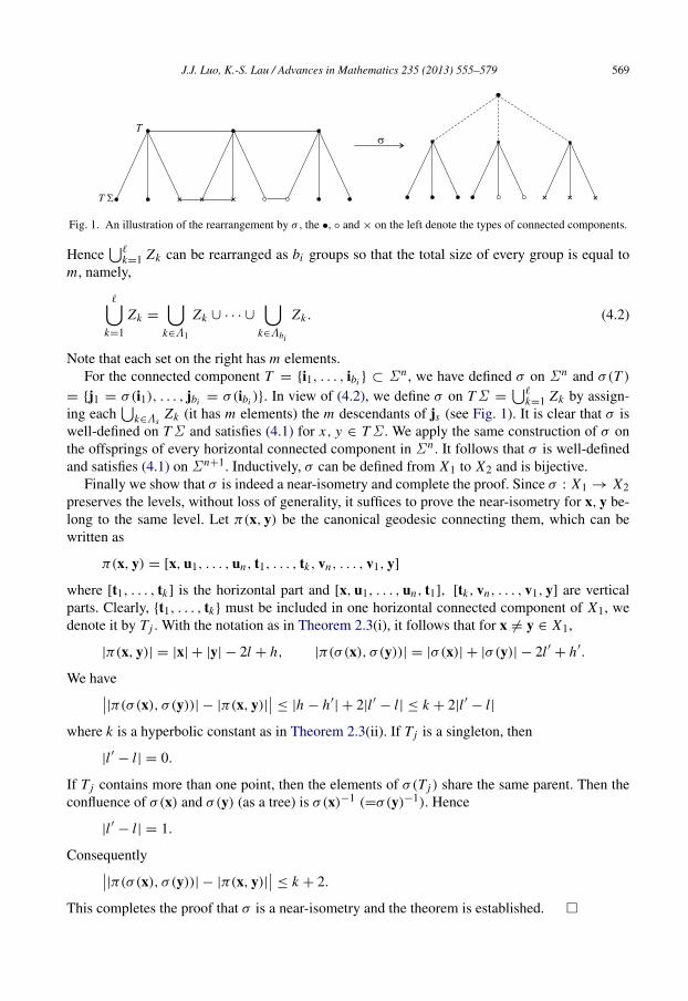
Fig. 1. An illustration of the rearrangement by σ , the •, and × on the left denote the types of connected components.

Henceℓ

k=1 Zk can be rearranged as bi groups so that the total size of every group is equal tom, namely,

ℓk=1

Zk =

k∈Λ1

Zk ∪ · · · ∪

k∈Λbi

Zk . (4.2)

Note that each set on the right has m elements.For the connected component T = i1, . . . , ibi ⊂ Σ n , we have defined σ on Σ n and σ(T )

= j1 = σ(i1), . . . , jbi = σ(ibi ). In view of (4.2), we define σ on TΣ =ℓ

k=1 Zk by assign-ing each

k∈Λs

Zk (it has m elements) the m descendants of js (see Fig. 1). It is clear that σ iswell-defined on TΣ and satisfies (4.1) for x, y ∈ TΣ . We apply the same construction of σ onthe offsprings of every horizontal connected component in Σ n . It follows that σ is well-definedand satisfies (4.1) on Σ n+1. Inductively, σ can be defined from X1 to X2 and is bijective.

Finally we show that σ is indeed a near-isometry and complete the proof. Since σ : X1 → X2preserves the levels, without loss of generality, it suffices to prove the near-isometry for x, y be-long to the same level. Let π(x, y) be the canonical geodesic connecting them, which can bewritten as

π(x, y) = [x, u1, . . . , un, t1, . . . , tk, vn, . . . , v1, y]

where [t1, . . . , tk] is the horizontal part and [x, u1, . . . , un, t1], [tk, vn, . . . , v1, y] are verticalparts. Clearly, t1, . . . , tk must be included in one horizontal connected component of X1, wedenote it by T j . With the notation as in Theorem 2.3(i), it follows that for x = y ∈ X1,

|π(x, y)| = |x| + |y| − 2l + h, |π(σ(x), σ (y))| = |σ(x)| + |σ(y)| − 2l ′ + h′.

We have|π(σ(x), σ (y))| − |π(x, y)| ≤ |h − h′

| + 2|l ′ − l| ≤ k + 2|l ′ − l|

where k is a hyperbolic constant as in Theorem 2.3(ii). If T j is a singleton, then

|l ′ − l| = 0.

If T j contains more than one point, then the elements of σ(T j ) share the same parent. Then theconfluence of σ(x) and σ(y) (as a tree) is σ(x)−1 (=σ(y)−1). Hence

|l ′ − l| = 1.

Consequently|π(σ(x), σ (y))| − |π(x, y)| ≤ k + 2.

This completes the proof that σ is a near-isometry and the theorem is established.


Corollary 4.5. Under the same assumption of Theorem 3.7. If there exists k ∈ N such that Ak is(mk, b)-rearrangeable, then ∂(X, E ) ≃ ∂(X, Ev).

To prove of Theorem 3.8 that primitive implies (m, b)-rearrangeable, we need a combinatoriallemma due to Xi and Xiong [24]. We include their proof for completeness.

Lemma 4.6. Let p, m and ni i∈Λ be positive integers with

i∈Λ ni = pm. Suppose thereexists an integer l with ni ≤ l < m for all i ∈ Λ, and #i ∈ Λ : ni = 1 ≥ pl. Then there is adecomposition Λ =

ps=1 Λs satisfying

i∈Λs

ni = m for 1 ≤ s ≤ p.

Proof. The lemma is trivially true for p = 1, suppose it is true for p. For p + 1, let Ω ⊂ i :

ni = 1 with #Ω = (p + 1)l, and select a maximal subset ∆1 of Λ \Ω such that

i∈∆1ni < m.

We claim thati∈∆1

ni ≥ m − l.

For otherwise, take i0 ∈ Λ \ (∆1 ∪ Ω), then

i∈∆1∪i0ni < (m − l) + l = m, which con-

tradicts the maximality of ∆1 and the claim follows. Choose a subset Ω1 from Ω such that#Ω1 = m −

i∈∆1

ni (≤ l) and set Λ1 = ∆1 ∪ Ω1, then

i∈Λ1ni = m.

Note that for Λ′= Λ \ Λ1, #i ∈ Λ′

: ni = 1 ≥ pl. Applying the inductive hypothesis on p,we get a decomposition Λ′

=p+1

s=2 Λs with

i∈Λsni = m for s ≥ 2. Therefore, the assertion

for p + 1 holds, and the lemma is proved.

Lemma 4.6 yields the following rearrangement lemma we need (see also [4]).

Lemma 4.7. Let b = [b1, . . . , br ]t∈ Nr with b1 = 1. Let ℓ = max j b j and a = [a1, . . . , ar ] ∈

Zr+ such that a1 ≥ ℓ2. Suppose there exists m > ℓ such that ab = pm for some integer

0 < p ≤ ℓ, then a is (m, b)-rearrangeable.

Proof. We first assume that all ai > 0. By the assumption, we have ℓ < m and a1 ≥ ℓ2≥ pℓ.

Define a sequence n j rj=1 by

n j =

b1 j = 1, . . . , a1;

b2 j = a1 + 1, . . . , a1 + a2;

...

br j =

r−1j=1

a j + 1, . . . ,

rj=1

a j .

Note that n j ≤ ℓ. Let Λ = 1, 2, . . . ,r

j=1 a j be the index set. Then the assumption ab = pmis equivalent to:

j∈Λ

n j = pm.

By Lemma 4.6, there is a decomposition Λ =p

s=1 Λs satisfying

j∈Λsn j = m for 1 ≤ s ≤ p.

Counting the number of b j ’s in each group s,


cs j = #k ∈ Λs : nk = b j , 1 ≤ s ≤ p, 1 ≤ j ≤ r.

The lemma follows by letting the matrix C = [cs j ]p×r .If some of the ai equals zero. Without loss generality we assume that ar = 0 and ai >

0, 1 ≤ i ≤ r − 1. Let a′= [a1, . . . , ar−1] and b′

= [b1, . . . , br−1], then a′b′= pm and

by the above conclusion, a′ is (m, b)-rearrangeable by a p × (r − 1) matrix C ′. Let C be thep × r matrix obtained by adding a last column 0 to C ′. Then it is easy to see that a is (m, b)-rearrangeable.

Proposition 4.8. Let A be an r × r nonnegative integral matrix and is primitive (i.e., An > 0for some n > 0). Let b = [b1, . . . , br ]

t∈ Nr with b1 = 1 and Ab = mb for some m ∈ N. Then

Ak is (mk, b)-rearrangeable for some k > 0.

Proof. Let ℓ = max j b j . Observe that A is primitive, there exists a large k such that ℓ <

mk , and Ak > 0 with every entry greater than ℓ2. Hence Lemma 4.7 implies Ak is (mk, b)-rearrangeable.

Proof of Theorem 3.8. Let A be the incidence matrix, and Ab = mb where b = [b1, . . . , br ]t

with bi = #T where [T ] = Ti (Proposition 3.6). If we let the root o to be T1, then it is clearfrom the definitions of A, b and Ab = mb that b1 = 1. Hence Proposition 4.8 implies that Ak is(mk, b)-rearrangeable for some k > 0.

To prove the last part, we can assume without loss of generality that A is (m, b)-rearrangeableand maxi bi ≤ m. For otherwise, by the primitive assumption on A and by the same reasoningas in the proof of Theorem 3.7, we can consider the augmented tree as the IFS defined by thek-th iteration of Si

mi=1, and the corresponding Ak is (mk, b)-rearrangeable. Hence we can apply

Theorem 3.7 and complete the proof of Theorem 3.8.

5. Examples

In this section, we provide several examples to illustrate our theorems of simple augmentedtree and Lipschitz equivalence. Note that all the IFS’s considered here satisfy condition (H);also the bounded closed invariant sets J we use are connected tiles and they have finite numberof neighbors. By using the following lemma, we see that the process of finding the connectedcomponents will end in finitely many steps.

We assume the IFS consists of contractive similitudes Si (x) = B−1(x + di ), i = 1, . . . , m,where B−1

= r R is the scaled orthogonal matrix. Let J be a closed subset such that Si (J ) ⊂ Jfor each i . Then for i = i1 · · · ik ∈ Σ k , we have Ji = Si(J ) = B−k(J + di) wheredi = dik + Bdik−1 + · · · + Bk−1di1 .

Lemma 5.1. For two horizontal connected components T1 ⊂ Σ k1 , T2 ⊂ Σ k2 with #T1 = #T2 =

ℓ. If there exist similitudes φi (x) = Bki x + ci , i = 1, 2, where ci ∈ Rd such that

φ1(∪i∈T1 Ji) = φ2(∪j∈T2 Jj) = J ∪ (J + v1) ∪ · · · ∪ (J + vℓ−1)

for some vectors v1, . . . , vℓ−1 ∈ Rd , then T1 ∼ T2.

Proof. By the definition and (3.1), it suffices to prove T1Σ and T2Σ have the same connectednessstructure, equivalently, to prove this for

i∈T1

mi=1 Jii and

j∈T2

mj=1 Jj j . Letting v0 = 0, we


have

φ1

i∈T1

mi=1

Jii

= Bk1

i∈T1

mi=1

Jii

+ c1

= Bk1

i∈T1

mi=1

B−k1−1(J + di + Bdi)

+ c1

=

i∈T1

mi=1

(Ji + di) + c1 =

ℓ−1j=0

mi=1

(Ji + v j ).

Similarly we have φ2

j∈T2

mj=1 Jj j

=ℓ−1

j=0m

i=1(Ji +v j ). Since φ1, φ2 are similarity mapswhich preserve the connectedness, the lemma follows.

We remark that it is a lot simpler to use the approach here than the method of constructing thegraph directed system as in [4,18,24]. In fact Example 5.4 shows that it may be difficult to usethe later to prove the Lipschitz equivalence. The same example also shows that the converse ofthe above lemma does not hold.

Example 5.2. Let D1 = 0, 2, 4 and D2 = 0, 3, 4 be two digit sets, and let K1 and K2 be thetwo self-similar sets defined by:

K1 =15(K1 + D1), K2 =

15(K2 + D2).

Then K1 is clearly dust-like and K1 ≃ K2 (see Fig. 2).

This is a well-known example of Lipschitz equivalence of self-similar sets called the 1, 3, 5–1, 4, 5 problem [3,18], which was proved by showing that they have the same graph directedsystem. In our approach, the associated augmented tree for K1 is just the standard rooted tree withno horizontal edges, and the incidence matrix is [3]. For K2, by letting Si (x) = (x + di )/3, di ∈

D2, and use J = [0, 1] in the definition of the augmented tree, we see that in total, there arethree connected classes (after three iterations): T1 = [o], T2 = [2, 3] and T3 = [22, 23, 31].Hence X is simple and the incidence matrix is

A =

1 1 01 1 11 1 2

.

Clearly A is primitive, and K2 ≃ K1 by Theorem 3.10. The following proposition is a generalization of Example 5.2 on R [18].

Proposition 5.3. Let D be a proper subset of 0, 1, . . . , n − 1, and let K the self-similar set onR satisfying

K =1n(K + D).

Then the corresponding augmented tree is simple and the incidence matrix is primitive.Consequently K is Lipschitz equivalent to a dust-like set.


a b

Fig. 2.

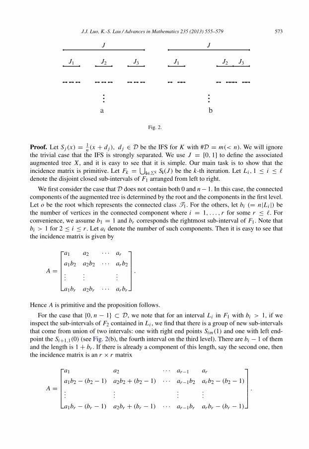
Proof. Let S j (x) =1n (x + d j ), d j ∈ D be the IFS for K with #D = m(< n). We will ignore

the trivial case that the IFS is strongly separated. We use J = [0, 1] to define the associatedaugmented tree X , and it is easy to see that it is simple. Our main task is to show that theincidence matrix is primitive. Let Fk =

i∈Σ k Si(J ) be the k-th iteration. Let L i , 1 ≤ i ≤ ℓ

denote the disjoint closed sub-intervals of F1 arranged from left to right.

We first consider the case that D does not contain both 0 and n −1. In this case, the connectedcomponents of the augmented tree is determined by the root and the components in the first level.Let o be the root which represents the connected class T1. For the others, let bi (= n|L i |) bethe number of vertices in the connected component where i = 1, . . . , r for some r ≤ ℓ. Forconvenience, we assume b1 = 1 and br corresponds the rightmost sub-interval of F1. Note thatbi > 1 for 2 ≤ i ≤ r . Let ai denote the number of such components. Then it is easy to see thatthe incidence matrix is given by

A =

a1 a2 · · · ar

a1b2 a2b2 · · · ar b2

......

...

a1br a2br · · · ar br

.

Hence A is primitive and the proposition follows.

For the case that 0, n − 1 ⊂ D, we note that for an interval L i in F1 with bi > 1, if weinspect the sub-intervals of F2 contained in L i , we find that there is a group of new sub-intervalsthat come from union of two intervals: one with right end points Sim(1) and one with left end-point the Si+1,1(0) (see Fig. 2(b), the fourth interval on the third level). There are bi − 1 of themand the length is 1 + br . If there is already a component of this length, say the second one, thenthe incidence matrix is an r × r matrix

A =

a1 a2 · · · ar−1 ar

a1b2 − (b2 − 1) a2b2 + (b2 − 1) · · · ar−1b2 ar b2 − (b2 − 1)

......

......

a1br − (br − 1) a2br + (br − 1) · · · ar−1br ar br − (br − 1)

.


a b

Fig. 3. The first two iterations for K .

If this is a new component, then the incidence matrix is an (r + 1) × (r + 1) matrix with

A =

a1 a2 · · · ar−1 ar 0

a1b2 − (b2 − 1) a2b2 · · · ar−1b2 ar b2 − (b2 − 1) b2 − 1...

......

......

a1br − (br − 1) a2br · · · ar−1br ar br − (br − 1) br − 1

a1(1 + br ) − br a2(1 + br ) · · · ar−1(1 + br ) ar (1 + br ) − br br

.

Again, A is primitive that implies the proposition.

The above proposition also has a higher dimensional extension to the totally disconnectedfractal cubes of the form K =

1n (K + D) where D ⊂ 0, . . . , n − 1

d by Xi and Xiong [24]via constructing a more complicated graph directed system. Their result can also be put intothe framework of Theorem 3.8, we will omit the detail. In the following we will consider othertotally disconnected self-similar sets of more general forms.

The following shows that the S j (J )’s can have large overlaps (though the OSC is still satisfiedby Corollary 3.11). Moreover it shows that the converse of Lemma 5.1 does not hold.

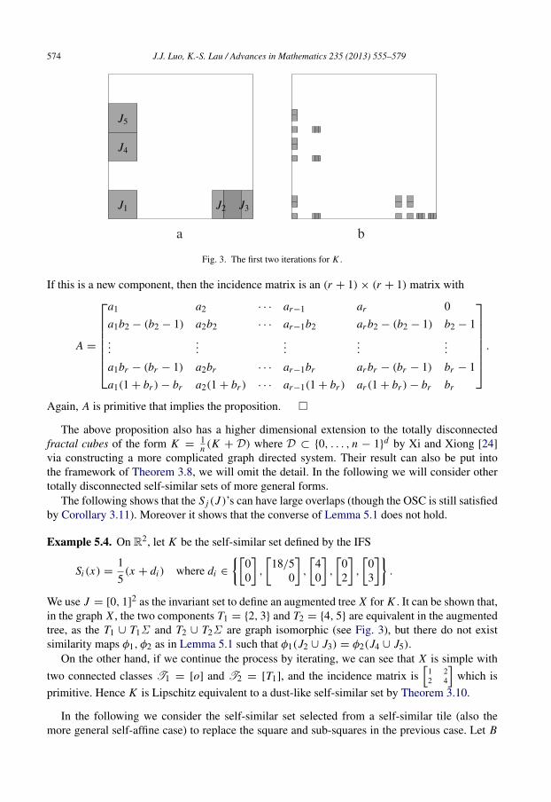
Example 5.4. On R2, let K be the self-similar set defined by the IFS

Si (x) =15(x + di ) where di ∈

00

,

18/5

0

,

40

,

02

,

03

.

We use J = [0, 1]2 as the invariant set to define an augmented tree X for K . It can be shown that,

in the graph X , the two components T1 = 2, 3 and T2 = 4, 5 are equivalent in the augmentedtree, as the T1 ∪ T1Σ and T2 ∪ T2Σ are graph isomorphic (see Fig. 3), but there do not existsimilarity maps φ1, φ2 as in Lemma 5.1 such that φ1(J2 ∪ J3) = φ2(J4 ∪ J5).

On the other hand, if we continue the process by iterating, we can see that X is simple with

two connected classes T1 = [o] and T2 = [T1], and the incidence matrix is

1 22 4

which is

primitive. Hence K is Lipschitz equivalent to a dust-like self-similar set by Theorem 3.10.

In the following we consider the self-similar set selected from a self-similar tile (also themore general self-affine case) to replace the square and sub-squares in the previous case. Let B


J1

J2

J3

J4

a b

Fig. 4.

be a d × d expanding matrix (i.e., all the eigenvalues have moduli > 1) and | det(B)| = q; letD = d1, . . . , dq ⊂ Rd be a digit set. The attractor J generated by

Si (x) = B−1(x + di ), di ∈ D

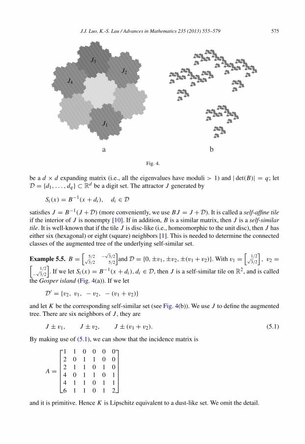
satisfies J = B−1(J + D) (more conveniently, we use B J = J + D). It is called a self-affine tileif the interior of J is nonempty [10]. If in addition, B is a similar matrix, then J is a self-similartile. It is well-known that if the tile J is disc-like (i.e., homeomorphic to the unit disc), then J haseither six (hexagonal) or eight (square) neighbors [1]. This is needed to determine the connectedclasses of the augmented tree of the underlying self-similar set.

Example 5.5. B =

5/2 −

√3/2

√3/2 5/2

and D = 0, ±v1, ±v2, ±(v1 + v2). With v1 =

1/2

√3/2

, v2 =

1/2−

√3/2

. If we let Si (x) = B−1(x + di ), di ∈ D, then J is a self-similar tile on R2, and is called

the Gosper island (Fig. 4(a)). If we let

D′= v2, v1, − v2, − (v1 + v2)

and let K be the corresponding self-similar set (see Fig. 4(b)). We use J to define the augmentedtree. There are six neighbors of J , they are

J ± v1, J ± v2, J ± (v1 + v2). (5.1)

By making use of (5.1), we can show that the incidence matrix is

A =

1 1 0 0 0 02 0 1 1 0 02 1 1 0 1 04 0 1 1 0 14 1 1 0 1 16 1 1 0 1 2

and it is primitive. Hence K is Lipschitz equivalent to a dust-like set. We omit the detail.


a b

Fig. 5.

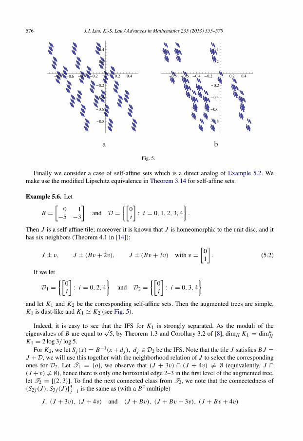
Finally we consider a case of self-affine sets which is a direct analog of Example 5.2. Wemake use the modified Lipschitz equivalence in Theorem 3.14 for self-affine sets.

Example 5.6. Let

B =

0 1

−5 −3

and D =

0i

: i = 0, 1, 2, 3, 4

.

Then J is a self-affine tile; moreover it is known that J is homeomorphic to the unit disc, and ithas six neighbors (Theorem 4.1 in [14]):

J ± v, J ± (Bv + 2v), J ± (Bv + 3v) with v =

01

. (5.2)

If we let

D1 =

0i

: i = 0, 2, 4

and D2 =

0i

: i = 0, 3, 4

and let K1 and K2 be the corresponding self-affine sets. Then the augmented trees are simple,K1 is dust-like and K1 ≃ K2 (see Fig. 5).

Indeed, it is easy to see that the IFS for K1 is strongly separated. As the moduli of theeigenvalues of B are equal to

√5, by Theorem 1.3 and Corollary 3.2 of [8], dimH K1 = dimw

HK1 = 2 log 3/ log 5.

For K2, we let S j (x) = B−1(x + d j ), d j ∈ D2 be the IFS. Note that the tile J satisfies B J =

J + D, we will use this together with the neighborhood relation of J to select the correspondingones for D2. Let T1 = o, we observe that (J + 3v) ∩ (J + 4v) = ∅ (equivalently, J ∩

(J +v) = ∅), hence there is only one horizontal edge 2–3 in the first level of the augmented tree,let T2 = [2, 3]. To find the next connected class from T2, we note that the connectedness ofS2 j (J ), S3 j (J )3

j=1 is the same as (with a B2 multiple)

J, (J + 3v), (J + 4v) and (J + Bv), (J + Bv + 3v), (J + Bv + 4v)


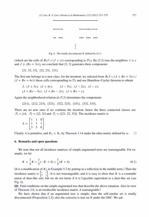
Fig. 6. The totally disconnected K defined by (6.1).

(which are the cells of B(J ∪ (J + v)) corresponding to D2). By (5.2) (use the neighbors J ± v

and J ± (Bv + 3v)), we conclude that 2, 3 generates three components

21, 32, 33, 22, 23, 31.

The first one belongs to a new class, for the iteration, we selected from B(J ∪ (J + Bv + 3v) ∪

(J + Bv + 4v)) those cells corresponding to D2 and use Hamilton–Cayley theorem to obtain

J, (J + 3v), (J + 4v); (J − 5v), (J − 2v), (J − v);

(J + Bv − 5v), (J + Bv − 2v), (J + Bv − v).

Again the neighborhood relation in (5.2) determines the components

211, 212, 213, 321, 322, 323, 331, 332, 333.

There are no new ones if we continue the iteration, hence the three connected classes are:T1 = [o], T2 = [2, 3] and T3 = [21, 32, 33]. The incidence matrix is

A =

1 1 01 1 13 3 0

.

Clearly A is primitive, and K2 ≃ K1 by Theorem 3.14 under the ultra-metric defined by w.

6. Remarks and open questions

We note that not all incidence matrices of simple augmented trees are rearrangeable. For ex-ample, we let

K =15

K ∪15(−K + 4) ∪

15(K + 4). (6.1)

(It is a modification of K2 in Example 5.2 by putting in a reflection in the middle term.) Then the

incidence matrix is

1 10 3

. It is not rearrangeable, and it is easy to show that K is a countable

union of dust-like sets, but we do not know if it is Lipschitz equivalent to a dust-like set (seeFig. 6).Q1. Find conditions on the simple augmented tree that describe the above situation. Also in viewof Theorem 3.8, is an irreducible incidence matrix A rearrangeable?

We have shown that if an augmented tree is simple, then the self-similar set is totallydisconnected (Proposition 2.5); also the converse is true on R under the OSC. We ask


Q2. Suppose K ⊂ Rd is defined by (2.2), if K is totally disconnected, does it imply that aug-mented tree is simple, equivalently, the horizontal connected component of the augmented treeis uniformly bounded (with or without assuming the OSC)?

In recent literature, the investigations of the Lipschitz equivalence are mainly for the fractalcubes of the form K =

1n (K + D) where D ⊂ 0, . . . , n − 1

d [24,25]. In Examples 5.5 and5.6, we bring in another classes of self-similar/self-affine sets K that are based on the disc-liketiles on R2. Note that such tiles have six or eight neighbors [1], and for such K , the augmentedtrees depend very much on this neighborhood relationship. For the self-affine tiles generated byconsecutive collinear digit sets, the disc-like property has been completely characterized in [14]through the characteristic polynomials of the expanding matrices. This provides a wealth ofsource to study the topological property of such K . A general question isQ3. For the classes of self-similar/self-affine sets K stated above, can we characterize the digitset D so that K is totally disconnected?

Also in [11], the authors have made a head start to investigate the classification of the non-totally disconnected fractal squares.Q4. Can we put such classification into the framework of augmented trees?

In our consideration, we have restricted the IFS to have equal contraction ratio. On the otherhand, there is also interesting study for different contraction ratios (e.g., [17,19,23]). For theaugmented tree, the setup in [12] is actually for non-equal contraction ratios that the horizontallevel Σ n can be replaced by the standard level set: Λn = i = i1 · · · ik : ri1 · · · rik ≤ rn <

ri1 · · · rik−1 where ri ’s are the contraction ratios. More generally, the authors have observed thatthe augmented trees can also be defined for Moran fractals and the hyperbolic property still holds.It is possible that the augmented trees can also be useful for the Lipschitz equivalence of fractalsets in those cases.

Acknowledgments

The authors would like to thank Professors De-Jun Feng, Xing-Gang He, Hui Rao andXiang-Yang Wang for many valuable comments and suggestions.

The research is supported by the HKRGC grant, the Focus Investment Scheme of CUHK, andthe NNSF of China (no. 10871065).

References

[1] C. Bandt, Y. Wang, Disklike self-affine tiles in R2, Discrete Comput. Geom. 26 (4) (2001) 591–601.[2] D. Cooper, T. Pignataro, On the shape of Cantor sets, J. Differential Geom. 28 (1988) 203-21.[3] G. David, S. Semmes, Fractured Fractals and Broken Dreams: Self-Similar Geometry through Metric and Measure,

Oxford Univ. Press, 1997.[4] G.T. Deng, X.G. He, Lipschitz equivalence of fractal sets in R, Sci. China Math. 55 (10) (2012) 2095–2107.[5] K.J. Falconer, D.T. Marsh, Classification of quasi-circles by Hausdorff dimension, Nonlinearity 2 (1989) 489–493.[6] K.J. Falconer, D.T. Marsh, On the Lipschitz equivalence of Cantor sets, Mathematika 39 (1992) 223–233.[7] M. Gromov, Hyperbolic groups, in: MSRI Publications 8, Springer Verlag, 1987, pp. 75–263.[8] X.G. He, K.S. Lau, On a generalized dimension of self-affine fractals, Math. Nachr. 281 (8) (2008) 1142–1158.[9] V.A. Kaimanovich, Random walks on Sierpinski graphs: hyperbolicity and stochastic homogenization, in: Fractals

in Graz 2001, in: Trends Math., Birkhuser, Basel, 2003, pp. 145–183.[10] J.C. Lagarias, Y. Wang, Self-affine tiles in Rn , Adv. Math. 121 (1996) 21–49.[11] K.S. Lau, J.J. Luo, H. Rao, Topological structure of fractal squares, Math. Proc. Camb. Phil. Soc. (in press).[12] K.S. Lau, X.Y. Wang, Self-similar sets as hyperbolic boundaries, Indiana Univ. Math. J. 58 (2009) 1777–1795.[13] K.S. Lau, X.Y. Wang, Self-similar sets, hyperbolic boundaries and Martin boundaries, Preprint.[14] K.S. Leung, K.S. Lau, Disk-likeness of planar self-affine tiles, Trans. Amer. Math. Soc. 359 (2007) 3337–3355.


[15] M. Llorente, P. Mattila, Lipschitz equivalence of subsets of self-conformal sets, Nonlinearity 23 (2010) 875–882.[16] P. Mattila, P. Saaranen, Ahlfors-David regular sets and bilipschitz maps, Ann. Acad. Sci. Fenn. Math. 34 (2009)

487–502.[17] H. Rao, H.J. Ruan, Y. Wang, Lipschitz equivalence of Cantor sets and algebraic properties of contraction ratios,

Trans. Amer. Math. Soc. 364 (2012) 1109–1126.[18] H. Rao, H.J. Ruan, L.-F. Xi, Lipschitz equivalence of self-similar sets, CR Acad. Sci. Paris, Ser. I 342 (2006)

191–196.[19] H.J. Ruan, Y. Wang, L. Xi, Lipschitz equivalence of self-similar sets with touching structures, Preprint.[20] A. Schief, Separation properties for self-similar sets, Proc. Amer. Math. Soc. 122 (1994) 111–115.[21] W. Woess, Random Walks on Infinite Graphs and Groups, in: Cambridge Tracts in Mathematics, vol. 138,

Cambridge University Press, Cambridge, 2000.[22] L.-F. Xi, Lipschitz equivalence of self-conformal sets, J. Lond. Math. Soc. 70 (2004) 369–382.[23] L.-F. Xi, H.J. Ruan, Lipschitz equivalence of generalized 1, 3, 5–1, 4, 5 self-similar sets, Sci. China Ser. A 50

(2007) 1537–1551.[24] L.-F. Xi, Y. Xiong, Self-similar sets with initial cubic patterns, CR Acad. Sci. Paris, Ser. I 348 (2010) 15–20.[25] L.-F. Xi, Y. Xiong, Lipschitz equivalence of fractals generated by nested cubes, Math. Z. 271 (2012) 1287–1308.

Documents

Lipschitz equivalence of self-similar sets and hyperbolic ...archive.ymsc.tsinghua.edu.cn/pacm_download/221/8454-Lipschitz... · Lipschitz equivalence of self-similar sets and hyperbolic