Lipschitz Properties for Deep Convolutional

Networks

Radu Balan∗, Maneesh Singh †, Dongmian Zou ‡

January 18, 2017

Abstract

In this paper we discuss the stability properties of convolutional neu-ral networks. Convolutional neural networks are widely used in machinelearning. In classification they are mainly used as feature extractors. Ide-ally, we expect similar features when the inputs are from the same class.That is, we hope to see a small change in the feature vector with respectto a deformation on the input signal. This can be established mathe-matically, and the key step is to derive the Lipschitz properties. Further,we establish that the stability results can be extended for more generalnetworks. We give a formula for computing the Lipschitz bound, andcompare it with other methods to show it is closer to the optimal value.

1 Introduction

Recently convolutional neural networks have enjoyed tremendous success inmany applications in image and signal processing. According to [5], a gen-eral convolutional network contains three types of layers: convolution layers,detection layers, and pooling layers. In [7], Mallat proposes the scattering net-work, which is a tree-structured convolutional neural network whose filters inconvolution layers are wavelets. Mallat proves that the scattering network sat-isfies two important properties: (approximately) invariance to translation andstabitity to deformation. However, for those properties to hold, the waveletsmust satisfy an admissibility condition. This restricts the adaptability of thetheory. The authors in [11, 12] use a slightly different setting to relax the condi-tions. They consider sets of filters that form semi-discrete frames of upper framebound equal to one. They prove that deformation stability holds for signals thatsatisfy certain conditions.

∗Department of Mathematics and Center for Scientific Computation and MathematicalModeling, University of Maryland, College Park, MD 20742 , rvbalan@math.umd.edu†Image and Video Analytics, Verisk Analytics, 545 Washington Boulevard, Jersey City, NJ

07310, Maneesh.Singh@verisk.com‡Department of Mathematics and Center for Scientific Computation and Mathematical

Modeling, University of Maryland, College Park, MD 20742, zou@math.umd.edu

1

In both settings, the deformation stability is a consequence of the Lipschitzproperty of the network, or feature extractor. The Lipschitz property in itselfis important even if we do not consider deformation of the form described in[7]. In [10], the authors detect some instability of the AlexNet by generatingimages that are easily recognizable by nude eyes but cause the network to giveincorrect classification results. They partially attribute the instability to thelarge Lipschitz bound of the AlexNet. It is thus desired to have a formula tocompute the Lipschitz bound in case the upper frame bound is not one.

The lower bound in the frame condition is not used when we analyze thestability properties for scattering networks. In [12] the authors conjecturedthat it has to do with the distinguishability of the two classes for classification.However, certain loss of information should be allowed for classification tasks.A lower frame bound is too strong in this case since it has most to do withinjectivity. In this paper, we only consider the semi-discrete Bessel sequence,and discuss a convolutional network of finite depth.

Merging is widely used in convolutional networks. Note that practitionersuse a concatenation layer ([9]) but that is just a concatenation of vectors and isof no mathematical interest. Nevertheless, aggregation by p-norms and multipli-cation is frequently used in networks and we still obtain stability to deformationin those cases and the Lipschitz bound increases only by a factor depending onthe number of filters to be aggregated.

The organization of this paper is as follows. In Section 2, we introducethe scattering network and state a general Lipschitz property. In Section 3,we discuss the aggregation of filters using p-norms or pointwise multiplication.In Section 4, we use examples of networks to compare different methods forcomputing the Lipschitz constants.

2 Scattering Network

We first review the theory developed by the authors in [7, 11, 12] and give a moregeneral result. Figure 1 shows a typical scattering network. f denotes an inputsignal (commonly in L2 or l2, for our discussion we take f ∈ L2(Rd)). gm,l’s andφm’s are filters and the corresponding blocks symbolizes the operation of doingconvolution with the filter in the block. The blocks marked σm,l illustrate theaction of a nonlinear function. This structure clearly shows the three stages ofa convolutional neural network: the gm,l’s are the convolution stage; the σm,l’sare the detection stage; the φm’s are the pooling stage.

The output of the network in Figure 1 is the collection of outputs of eachlayer. To represent the result clearly, we introduce some notations first.

We call an ordered collection of filters gm,l ∈ L1(Rd) connected in the net-work starting from m = 1 a path, say q = (g1,l1 , g2,l2 , · · · , gMq,lMq

) (for brevitywe also denote it as q = ((1, l1), (2, l2), · · · , (Mq, lMq

)), and in this case we de-note |q| = Mq to be the number of filters in the collection. We call |q| the lengthof the path. For q = ∅, we say that |q| = 0. The largest possible |q|, say M ,is called the depth of the network. For each m = 1, 2, · · · ,M + 1, there is an

2

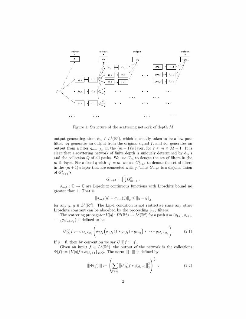
Figure 1: Structure of the scattering network of depth M

output-generating atom φm ∈ L1(Rd), which is usually taken to be a low-passfilter. φ1 generates an output from the original signal f , and φm generates anoutput from a filter gm−1,lm in the (m − 1)’s layer, for 2 ≤ m ≤ M + 1. It isclear that a scattering network of finite depth is uniquely determined by φm’sand the collection Q of all paths. We use Gm to denote the set of filters in them-th layer. For a fixed q with |q| = m, we use Gqm+1 to denote the set of filtersin the (m+ 1)’s layer that are connected with q. Thus Gm+1 is a disjoint unionof Gqm+1’s:

Gm+1 =⋃Gqm+1 .

σm,l : C → C are Lipschitz continuous functions with Lipschitz bound nogreater than 1. That is,

‖σm,l(y)− σm,l(y)‖2 ≤ ‖y − y‖2for any y, y ∈ L2(Rd). The Lip-1 condition is not restrictive since any otherLipschitz constant can be absorbed by the proceeding gm,l filters.

The scattering propagator U [q] : L2(Rd)→ L2(Rd) for a path q = (g1,l1 , g2,l2 ,· · · , gMq,lMq

) is defined to be

U [q]f := σMq,lMq

(σ2,l2

(σ1,l1(f ∗ g1,l1) ∗ g2,l2

)∗ · · · ∗ gMq,lMq

). (2.1)

If q = ∅, then by convention we say U [∅]f := f .Given an input f ∈ L2(Rd), the output of the network is the collections

Φ(f) := {U [q]f ∗ φMq+1}q∈Q. The norm ||| · ||| is defined by

|||Φ(f)||| :=

∑q∈Q

∥∥U [q]f ∗ φMq+1

∥∥22

12

. (2.2)

3

Given a collection of filters {gi}i∈I where the index set I is at most countableand for each i, gi ∈ L1(Rd) ∩ L2(Rd), {gi}i∈I is said to form the atoms of asemi-discrete Bessel sequence if there exists a constant B > 0 for which∑

i∈I‖f ∗ gi‖22 ≤ B ‖f‖

22

for any f ∈ L2. In this case, {gi}i∈I is said to form the atoms of a semi-discreteframe if in addition there exists a constant A > 0 for which

A ‖f‖22 ≤∑i∈I‖f ∗ gi‖22 ≤ B ‖f‖

22

for any f ∈ L2.Conditions (2.1) and (2.5) can be achieved for a larger class of filters. Specif-

ically, we shall introduce a Banach algebra in (3.1), where the Bessel bound isnaturally defined.

Throughout this paper, we adapt the definition of Fourier transform of afunction f to be

f(ω) =

∫Rdf(x)e−2πiωxdx . (2.3)

The dilation of f by a factor λ is defined by

fλ(x) = λf(λx) . (2.4)

The first result of this paper compiles and extends previous results obtainedin [7, 11, 12].

Theorem 2.1 (See also [7, 11, 12]). Suppose we have a scattering network ofdepth M . For each m = 1, 2, · · · ,M + 1,

Bm = maxq:|q|=m−1

∥∥∥∥∥∥( ∑gm,l∈Gqm

|gm,l|2)

+∣∣∣φm∣∣∣2

∥∥∥∥∥∥∞

<∞ (2.5)

with the understanding that BM+1 =∥∥∥φM+1

∥∥∥2∞

(that is, GqM+1 = ∅). Then

the corresponding feature extractor Φ is Lipschitz continuous in the followingmanner:

|||Φ(f)− Φ(h)||| ≤

(M+1∏m=1

Bm

) 12

‖f − h‖2 ,

whereB1 = B1, Bm = max{1, Bm} for m ≥ 2 . (2.6)

Proof. First we prove a lemma.

4

Lemma 2.2. With the settings in Theorem 2.1, for 0 ≤ m ≤M − 1, we have∑|q|=m+1

‖U [q]f − U [q]h‖22 +∑|q|=m

‖U [q]f ∗ φm+1 − U [q]h ∗ φm+1‖22

≤∑|q|=m

Bm+1 ‖U [q]f − U [q]h‖22 ;(2.7)

for m = M , we have∑|q|=M

‖U [q]f ∗ φm+1 − U [q]h ∗ φm+1‖22 ≤∑|q|=M

BM+1 ‖U [q]f − U [q]h‖22 .

(2.8)

Proof of Lemma 2.2. Let q be a path with |q| = m < M . We go one layerdeeper to get∑

q′∈q×Gqm+1

‖U [q′]f − U [q′]h‖22 + ‖U [q]f ∗ φm+1 − U [q]h ∗ φm+1‖22

=∑

gm+1,l∈Gqm+1

‖σm+1,l(U [q]f ∗ gm+1,l)− σm+1,l(U [q]h ∗ gm+1,l)‖22 +

‖U [q]f ∗ φm+1 − U [q]h ∗ φm+1‖22≤

∑gm+1,l∈Gqm+1

‖U [q]f ∗ gm+1,l − U [q]h ∗ gm+1,l‖22 + ‖U [q]f ∗ φm+1 − U [q]h ∗ φm+1‖22

=∑

gm+1,l∈Gqm+1

‖(U [q]f − U [q]h) ∗ gm+1,l‖22 + ‖(U [q]f − U [q]h) ∗ φm+1‖22 .

(2.9)Sum over all q with length m, we have∑

|q|=m+1

‖U [q]f − U [q]h‖22 +∑|q|=m

‖U [q]f ∗ φm+1 − U [q]h ∗ φm+1‖22

≤∑|q|=m

∑gm+1,l∈Gm+1

‖(U [q]f − U [q]h) ∗ gm+1,l‖22 +

∑|q|=m

‖U [q]f ∗ φm+1 − U [q]h ∗ φm+1‖22

≤∑|q|=m

Bm+1 ‖U [q]f − U [q]h‖22 ,

(2.10)

which follows the Bessel inequality by the definition of the Bm’s. For m = M,directly following the Young’s inequality we have (2.8).

We now continue with the proof of Theorem 2.1. The inqualities (2.7) and

5

(2.8) have two consequences. First, summing over m = 0, · · · ,M we have

M∑m=0

∑|q|=m

‖U [q]f ∗ φm+1 − U [q]h ∗ φm+1‖22

≤ B1 ‖f − h‖22 +

M∑m=1

(Bm+1 − 1)∑|q|=m

‖U [q]f − U [q]h‖22 ;

(2.11)

second, we have for each m = 0, · · · ,M − 1 that∑|q|=m+1

‖U [q]f − U [q]h‖22 ≤∑|q|=m

Bm+1 ‖U [q]f − U [q]h‖22 . (2.12)

Therefore, put (2.11) and (2.12) together, noting that Bm ≤ Bm for each m, wehave

M∑m=0

∑|q|=m

‖U [q]f ∗ φm+1 − U [q]h ∗ φm+1‖22

≤ B1 ‖f − h‖22 +

M∑m=1

(Bm+1 − 1)

(m∏

m′=1

Bm′

)‖f − h‖22

≤

(M+1∏m=1

Bm

)‖f − h‖22 .

(2.13)

We complete the proof by observing that the uppermost object in Inequality(2.13) is nothing but |||Φ(f)− Φ(h)|||2.

Remark 2.3. [11, 12] consider the case where each filter in the m-th layer inconnected to all the frame vectors from the pre-designed frame for the (m+ 1)-th layer. In practical uses then, a dimension reduction process needs to be doneto select a few branches from the numerous tributaries due to such a designmanner (see [1]). Also, the authors of [11, 12] assume that all the Bm’s are lessthan or equal to one. As can be seen in the above proof, this assumption is notneeded.

Remark 2.4. The infinite-depth case is an immediate extension of the finite-depth case if

∏Bm <∞.

Theorem 2.1, together with Schur’s test (for integral operators), lead to thefollowing theorem, which implies the deformation stability of the correspondingnetwork. The proof can be found in [11]. We state this result for the complete-ness of this article.

Theorem 2.5 ([11]). With the settings in Theorem 2.1, Let HR be the space ofR-band-limited functions defined by

HR := {f ∈ L2(Rd) : supp(f) ⊂ BR(0)} .

6

Then for all f ∈ HR, ω ∈ C(Rd, R), τ ∈ C1(Rd, R) with ‖Dτ‖∞ ≤ (2d)−1,

|||Φ(f)− Φ(Fτ,ωf)||| ≤ C(R ‖τ‖∞ + ‖ω‖∞) ‖f‖2 ,

where Fτ,ωf) is the deformed version of f defined by

Fτ,ωf(x) := e2πiω(x)f(x− τ(x)) . (2.14)

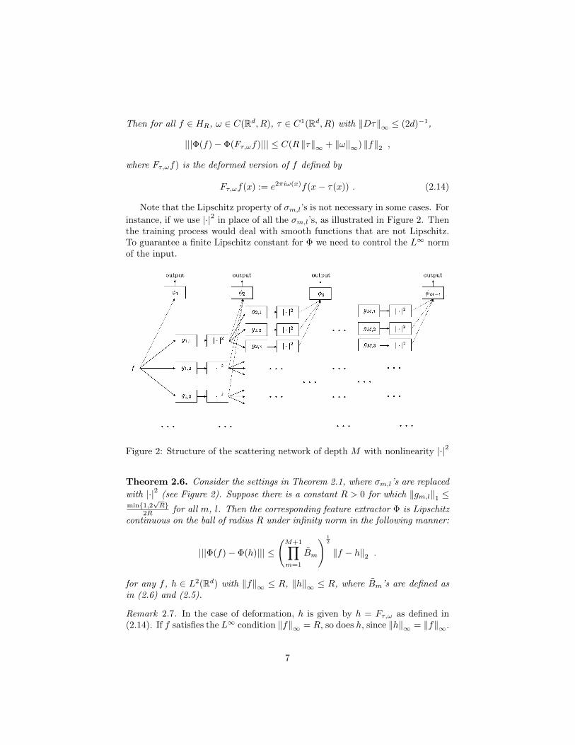
Note that the Lipschitz property of σm,l’s is not necessary in some cases. For

instance, if we use |·|2 in place of all the σm,l’s, as illustrated in Figure 2. Thenthe training process would deal with smooth functions that are not Lipschitz.To guarantee a finite Lipschitz constant for Φ we need to control the L∞ normof the input.

Figure 2: Structure of the scattering network of depth M with nonlinearity |·|2

Theorem 2.6. Consider the settings in Theorem 2.1, where σm,l’s are replaced

with |·|2 (see Figure 2). Suppose there is a constant R > 0 for which ‖gm,l‖1 ≤min{1,2

√R}

2R for all m, l. Then the corresponding feature extractor Φ is Lipschitzcontinuous on the ball of radius R under infinity norm in the following manner:

|||Φ(f)− Φ(h)||| ≤

(M+1∏m=1

Bm

) 12

‖f − h‖2 .

for any f , h ∈ L2(Rd) with ‖f‖∞ ≤ R, ‖h‖∞ ≤ R, where Bm’s are defined asin (2.6) and (2.5).

Remark 2.7. In the case of deformation, h is given by h = Fτ,ω as defined in(2.14). If f satisfies the L∞ condition ‖f‖∞ = R, so does h, since ‖h‖∞ = ‖f‖∞.

7

Proof. Notice that min{1,2√R}

2R = min{ 1√R, 12R}. Hence ‖gm,l‖1 ≤ 1/

√R and

‖gm,l‖1 ≤ 1/2R. We observe that for any path q with length |q| = m ≥ 1, sayq =

((1, l1), (2, l2), · · · , (Mq, lMq

)), and for convenience denote q1 = ((1, l1)),

q2 = ((1, l1), (2, l2)), · · · , qMq−1 =((1, l1), (2, l2), · · · , (Mq − 1, lMq−1)

), we have

‖U [q]f‖∞ =

∥∥∥∥∣∣∣U [qMq−1]f ∗ gMq,lMq

∣∣∣2∥∥∥∥∞

≤∥∥U [qMq−1]f

∥∥2∞

∥∥∥gMq,lMq

∥∥∥21

≤∥∥U [qMq−2]f

∥∥4∞

∥∥∥gMq−1,lMq−1

∥∥∥41

∥∥∥gMq,lMq

∥∥∥21

≤ · · ·

≤ ‖U [q1]f‖2Mq−1

∞

Mq∏j=2

∥∥gj,lj∥∥2Mq−j+1

1

≤ ‖f‖2Mq

∞

Mq∏j=1

∥∥gj,lj∥∥2Mq−j+1

1

≤ R2MqMq∏j=1

(1√R

)2Mq−j+1

= R2Mq ·(

1√R

)(2Mq−1)

= R .

With this, let q be a path of length |q| = m < M , we have for each l that∥∥∥|U [q]f ∗ gm+1,l|2 − |U [q]h ∗ gm+1,l|2∥∥∥22

= ‖(|U [q]f ∗ gm+1,l|+ |U [q]h ∗ gm+1,l|) (|U [q]f ∗ gm+1,l| − |U [q]h ∗ gm+1,l|)‖22≤ ‖|U [q]f ∗ gm+1,l|+ |U [q]h ∗ gm+1,l|‖21 ‖|U [q]f ∗ gm+1,l| − |U [q]h ∗ gm+1,l|‖22≤ (‖U [q]f‖∞ + ‖U [q]h‖∞)

2 ‖gm+1,l‖21 ‖|U [q]f ∗ gm+1,l| − |U [q]h ∗ gm+1,l|‖22≤ (R+R)2(1/2R)2 ‖|U [q]f ∗ gm+1,l| − |U [q]h ∗ gm+1,l|‖22= ‖|U [q]f ∗ gm+1,l| − |U [q]h ∗ gm+1,l|‖22≤ ‖U [q]f ∗ gm+1,l − U [q]h ∗ gm+1,l‖22 .

8

Therefore,∑q′∈q×Gqm+1

‖U [q′]f − U [q′]h‖22 + ‖U [q]f ∗ φm+1 − U [q]h ∗ φm+1‖22

≤∑

gm+1,l∈Gqm+1

‖U [q]f ∗ gm+1,l − U [q]h ∗ gm+1,l‖22 + ‖U [q]f ∗ φm+1 − U [q]h ∗ φm+1‖22

=∑

gm+1,l∈Gqm+1

‖(U [q]f − U [q]h) ∗ gm+1,l‖22 + ‖(U [q]f − U [q]h) ∗ φm+1‖22 .

Then by exactly the same inequality as (2.10), for 0 ≤ m ≤M − 1,∑|q|=m+1

‖U [q]f − U [q]h‖22 +∑|q|=m

‖U [q]f ∗ φm+1 − U [q]h ∗ φm+1‖22

≤∑|q|=m

Bm+1 ‖U [q]f − U [q]h‖22 ;

and for m = M ,∑|q|=M

‖U [q]f ∗ φm+1 − U [q]h ∗ φm+1‖22 ≤∑|q|=M

BM+1 ‖U [q]f − U [q]h‖22 .

The rest of the proof is a minimal modification to that of Theorem 2.1. Itis obvious that ‖f‖∞ = ‖Fτ,ω‖∞.

In most applications, the L∞-norm of the input is well bounded. For in-stance, normalized grayscale images have pixel valued between 0 and 1. Even ifit is not the case, we can pre-filter the input by widely used sigmoid functions,such as tanh. For instance, in the above case of |·|2, we can use the structure asfollows.

Figure 3: Restrict ‖f‖∞ at the first layer using R · tanh

3 Filter Aggregation

3.1 Aggregation by taking norm across filters

We use filter aggregation to model the pooling stage after convolution. In deeplearning there are two widely used pooling operation, max pooling and averagepooling. Max pooling is the operation of extracting local maximum of the signal,and can be modeled by an L∞-norm aggregation of copies of shifted and dilatedsignals. Average pooling is the operation of taking local average of the signal,

9

and can be modeled by a L1-norm aggregation of copies of shifted and dilatedsignals. When those pooling operations exist, it is still desired that the featureextractor is stable. We analyze this type of aggregation in detail as follows.

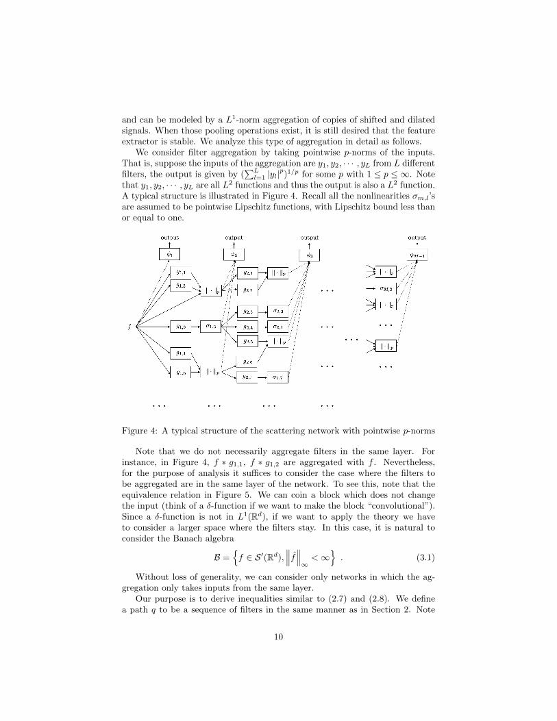
We consider filter aggregation by taking pointwise p-norms of the inputs.That is, suppose the inputs of the aggregation are y1, y2, · · · , yL from L differentfilters, the output is given by (

∑Ll=1 |yl|

p)1/p for some p with 1 ≤ p ≤ ∞. Note

that y1, y2, · · · , yL are all L2 functions and thus the output is also a L2 function.A typical structure is illustrated in Figure 4. Recall all the nonlinearities σm,l’sare assumed to be pointwise Lipschitz functions, with Lipschitz bound less thanor equal to one.

Figure 4: A typical structure of the scattering network with pointwise p-norms

Note that we do not necessarily aggregate filters in the same layer. Forinstance, in Figure 4, f ∗ g1,1, f ∗ g1,2 are aggregated with f . Nevertheless,for the purpose of analysis it suffices to consider the case where the filters tobe aggregated are in the same layer of the network. To see this, note that theequivalence relation in Figure 5. We can coin a block which does not changethe input (think of a δ-function if we want to make the block “convolutional”).Since a δ-function is not in L1(Rd), if we want to apply the theory we haveto consider a larger space where the filters stay. In this case, it is natural toconsider the Banach algebra

B ={f ∈ S ′(Rd),

∥∥∥f∥∥∥∞<∞

}. (3.1)

Without loss of generality, we can consider only networks in which the ag-gregation only takes inputs from the same layer.

Our purpose is to derive inequalities similar to (2.7) and (2.8). We definea path q to be a sequence of filters in the same manner as in Section 2. Note

10

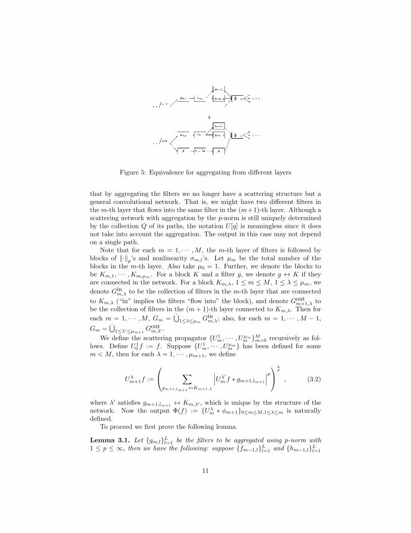
Figure 5: Equivalence for aggregating from different layers

that by aggregating the filters we no longer have a scattering structure but ageneral convolutional network. That is, we might have two different filters inthe m-th layer that flows into the same filter in the (m+1)-th layer. Although ascattering network with aggregation by the p-norm is still uniquely determinedby the collection Q of its paths, the notation U [q] is meaningless since it doesnot take into account the aggregation. The output in this case may not dependon a single path.

Note that for each m = 1, · · · ,M , the m-th layer of filters is followed byblocks of ‖·‖p’s and nonlinearity σm,l’s. Let µm be the total number of theblocks in the m-th layer. Also take µ0 = 1. Further, we denote the blocks tobe Km,1, · · · ,Km,µm . For a block K and a filter g, we denote g ↔ K if theyare connected in the network. For a block Km,λ, 1 ≤ m ≤ M , 1 ≤ λ ≤ µm, we

denote Ginm,λ to be the collection of filters in the m-th layer that are connected

to Km,λ (“in” implies the filters “flow into” the block), and denote Goutm+1,λ to

be the collection of filters in the (m+ 1)-th layer connected to Km,λ. Then for

each m = 1, · · · ,M , Gm =⋃

1≤λ≤µm Ginm,λ; also, for each m = 1, · · · ,M − 1,

Gm =⋃

1≤λ′≤µm+1Goutm,λ′ .

We define the scattering propagator {U1m, · · · , Uµmm }Mm=0 recursively as fol-

lows. Define U10 f := f . Suppose {U1

m, · · · , Uµmm } has been defined for somem < M , then for each λ = 1, · · · , µm+1, we define

Uλm+1f :=

∑gm+1,lm+1

↔Km+1,λ

∣∣∣Uλ′m f ∗ gm+1,lm+1

∣∣∣p 1

p

, (3.2)

where λ′ satisfies gm+1,lm+1↔ Km,λ′ , which is unique by the structure of the

network. Now the output Φ(f) := {Uλm ∗ φm+1}0≤m≤M,1≤λ≤m is naturallydefined.

To proceed we first prove the following lemma.

Lemma 3.1. Let {gm,l}Ll=1 be the filters to be aggregated using p-norm with1 ≤ p ≤ ∞, then we have the following: suppose {fm−1,l}Ll=1 and {hm−1,l}Ll=1

11

are two sets of inputs to those filters and fm and hm are the outputs respectively,then

‖fm − hm‖22 ≤ max(1, L2/p−1)

L∑l=1

‖(fm−1,l − hm−1,l) ∗ gm,l‖22 . (3.3)

Proof. For 1 ≤ p ≤ ∞, applying∣∣∣‖v1‖p − ‖v2‖p∣∣∣ ≤ ‖v1 − v2‖p and ‖v1‖p ≤

max(1, L1/p−1/2) ‖v1‖2 for any vectors v1, v2 of length L, we have

‖fm − hm‖22 =

∥∥∥∥∥∥(

L∑l=1

|fm−1,l ∗ gm,l|p)1/p

−

(L∑l=1

|hm−1,l ∗ gm,l|p)1/p

∥∥∥∥∥∥2

2

≤

∥∥∥∥∥∥(

L∑l=1

|(fm−1,l − hm−1,l) ∗ gm,l|p)1/p

∥∥∥∥∥∥2

2

≤

∥∥∥∥∥∥max(1, L1/p−1/2)

(L∑l=1

|(fm−1,l − hm−1,l) ∗ gm,l|2)1/2

∥∥∥∥∥∥2

2

= max(1, L2/p−1)

∫ L∑l=1

|(fm−1,l − hm−1,l) ∗ gm,l|2

= max(1, L2/p−1)

L∑l=1

‖(fm−1,l − hm−1,l) ∗ gm,l‖22 .

With Lemma 3.1 we can compute for any m = 0, · · · ,M that

µm+1∑λ=1

∥∥Uλm+1f − Uλm+1h∥∥22

≤µm∑λ′=1

∑l:gm+1,l∈Gout

m,λ′

max

(1,∣∣∣Gin

m+1,λ

∣∣∣2/p−1)∥∥∥Uλ′m f ∗ gm+1,l − Uλ′

m h ∗ gm+1,l

∥∥∥22,

where for each m, l, Ginm+1,λ is the unique class of filters that contains gm+1,l.

We can then proceed similar to Inequality (2.9) with minor changes. We getthe following result on the Lipschitz properties for Φ.

Theorem 3.2. Suppose we have a scattering network of depth M including onlyp-norm aggregations. For m = 1, 2, · · · ,M + 1, set

Bm = max1≤λ′≤µm−1

∥∥∥∥∥∥∥∑

l:gm,l∈Goutm,λ′

max

(1,∣∣∣Gin

m+1,λ

∣∣∣2/p−1) |gm,l|2 +∣∣∣φm∣∣∣2

∥∥∥∥∥∥∥∞

<∞

12

(with the understanding that BM+1 =∥∥∥φM+1

∥∥∥2∞

, that is, GoutM+1,λ′ = ∅ for any

1 ≤ λ′ ≤ µM ), where for each m, l, Ginm,λ is the unique class of filters that

contains gm,l and Ginm,λ denotes its cardinal. Then the corresponding feature

extractor Φ is Lipschitz continuous in the following manner:

|||Φ(f)− Φ(h)||| ≤

(M+1∏m=1

Bm

) 12

‖f − h‖2 , ∀f, h ∈ L2(Rd) ,

where Bm’s are defined as in (2.6) and (2.5).

3.2 Aggregation by pointwise multiplication

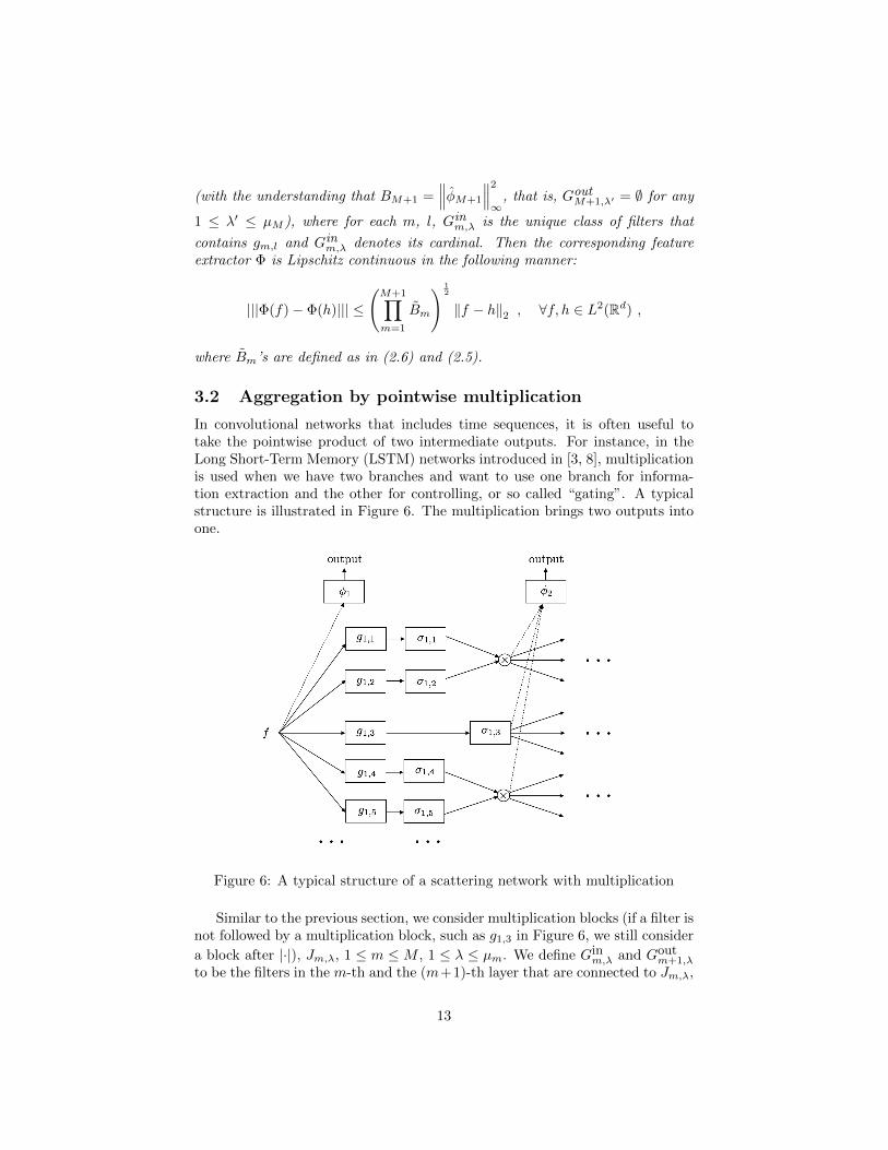
In convolutional networks that includes time sequences, it is often useful totake the pointwise product of two intermediate outputs. For instance, in theLong Short-Term Memory (LSTM) networks introduced in [3, 8], multiplicationis used when we have two branches and want to use one branch for informa-tion extraction and the other for controlling, or so called “gating”. A typicalstructure is illustrated in Figure 6. The multiplication brings two outputs intoone.

Figure 6: A typical structure of a scattering network with multiplication

Similar to the previous section, we consider multiplication blocks (if a filter isnot followed by a multiplication block, such as g1,3 in Figure 6, we still consider

a block after |·|), Jm,λ, 1 ≤ m ≤M , 1 ≤ λ ≤ µm. We define Ginm,λ and Gout

m+1,λ

to be the filters in the m-th and the (m+1)-th layer that are connected to Jm,λ,

13

respectively. Note that∣∣∣Gin

m,λ

∣∣∣ ∈ {1, 2}. The scattering propagator Uλm’s and

output generating operator Φ are defined similarly. The Lipschitz property isgiven by the following Theorem.

Theorem 3.3. Suppose we have a scattering network of depth M involving onlypointwise multiplication blocks. For m = 1, 2, · · · ,M + 1,

Bm = max1≤λ≤µm

∥∥∥∥∥∥∑

gm,l∈Goutm,λ

∣∣∣Ginm,λ

∣∣∣ |gm,l|2 +∣∣∣φm∣∣∣2

∥∥∥∥∥∥∞

<∞

(with the understanding that BM+1 =∥∥∥φM+1

∥∥∥2∞

, that is, GoutM+1,λ = ∅ for all

1 ≤ λ ≤ M), where for each m, l, Ginm,λ is the unique class of filters that

contains gm,l. Suppose ‖gm,l‖1 ≤ 1 for all m, l. Then the corresponding featureextractor Φ is Lipschitz continuous on the ball of radius 1 under infinity normin the following manner:

|||Φ(f)− Φ(h)||| ≤

(M+1∏m=1

Bm

) 12

‖f − h‖2 ,

for any f , h ∈ L2(Rd) with ‖f‖∞ ≤ 1, ‖h‖∞ ≤ 1, where Bm’s are defined as in(2.6) and (2.5).

This follows by minimal modification in the proof of Theorem 2.1 once weprove the following two lemmas. Lemma 3.4 implies that the infinite norm of theinputs to each layer have the same bound. Lemma 3.5 gives a similar inequalityto (2.9).

Lemma 3.4. (1) Let gm,1 and gm,2 be the two filters to be aggregated usingmultiplication with ‖gm,j‖1 ≤ 1 for j = 1, 2. We have the following: supposefm−1,1 and fm−1,2 are the inputs to the filters respectively with ‖fm−1,j‖∞ ≤ 1for j = 1, 2, then the output fm satisfies ‖fm‖∞ ≤ 1;(2) Let gm be a filter not to be aggregated with ‖gm‖1 ≤ 1, then suppose fm−1is the input to the filter with ‖fm−1‖∞ ≤ 1, we have the output fm satisfies‖fm‖∞ ≤ 1.

Proof. (2) directly follows from Young’s Inequality. For (1), we have

‖fm‖∞ = ‖σm,1(fm−1,1 ∗ gm,1) · σm,2(fm−1,2 ∗ gm,2)‖∞≤ ‖fm−1,1 ∗ gm,1‖∞ ‖fm−1,2 ∗ gm,2‖∞≤ ‖fm−1,1‖∞ ‖fm−1,2‖∞ ‖gm,1‖1 ‖gm,2‖1≤ 1 .

14

Lemma 3.5. Let gm,1, gm,2 be the two filters to be aggregated using a multi-plication block with ‖gm,j‖1 ≤ 1 for j = 1, 2. We have the following: suppose{fm−1,j}2j=1 and {hm−1,j}2j=1 are two sets of inputs to those filters with infinitenorm bounded by 1, and fm and hm are the outputs respectively, then

‖fm − hm‖22 ≤ 2 ‖(fm−1,1 − hm−1,1) ∗ gm,1‖22 + 2 ‖(fm−1,2 − hm−1,2) ∗ gm,2‖22 .

Proof.

‖fm − hm‖22= ‖σm,1(fm−1,1 ∗ gm,1)σm,2(fm−1,2 ∗ gm,2)−

σm,1(hm−1,1 ∗ gm,1)σm,2(hm−1,2 ∗ gm,2)‖22= ‖σm,1(fm−1,1 ∗ gm,1)σm,2(fm−1,2 ∗ gm,2)−

σm,1(fm−1,1 ∗ gm,1)σm,2(hm−1,2 ∗ gm,2)+

σm,1(fm−1,1 ∗ gm,1)σm,2(hm−1,2 ∗ gm,2)−σm,1(hm−1,1 ∗ gm,1)σm,2(hm−1,2 ∗ gm,2)‖22

≤ 2‖σm,1(fm−1,1 ∗ gm,1)σm,2(fm−1,2 ∗ gm,2)−σm,1(fm−1,1 ∗ gm,1)σm,2(hm−1,2 ∗ gm,2)‖22+

2‖σm,1(fm−1,1 ∗ gm,1)σm,2(hm−1,2 ∗ gm,2)−σm,1(hm−1,1 ∗ gm,1)σm,2(hm−1,2 ∗ gm,2)‖22

≤ 2‖σm,1(fm−1,1 ∗ gm,1)‖2∞‖σm,2(fm−1,2 ∗ gm,2)−σm,2(hm−1,2 ∗ gm,2)‖22+

2 ‖σm,2(hm−1,2 ∗ gm,2)‖2∞ ‖σm,1(fm−1,1 ∗ gm,1)−σm,1(hm−1,1 ∗ gm,1)‖22

≤ 2 ‖fm−1,1‖2∞ ‖gm,1‖21 ‖(fm−1,2 − hm−1,2) ∗ gm,2‖22 +

2 ‖hm−1,2‖2∞ ‖gm,2‖21 ‖(fm−1,1 − hm−1,1) ∗ gm,1‖22

≤ 2 ‖(fm−1,1 − hm−1,1) ∗ gm,1‖22 +

2 ‖(fm−1,2 − hm−1,2) ∗ gm,2‖22 .

For a general f ∈ L2(Rd), as discussed in the end of Section 2, we can first letit go through a sigmoid-like function, then go through the scattering network.

3.3 Mixed aggregations

The two types of aggregation blocks can be mixed together in the same net-works (which is the common case in applications). The precise statement ofthe Lipschitz property becomes a little cumbersome to state in full generality.However, L2-norm estimates can be combined using Theorem 2.1, 2.6, 3.2 and3.3. This is illustrated in the next section.

15

4 Examples of estimating the Lipschitz constant

We use three different approaches to estimate the Lipschitz constant. The firstis by propagating backward from the outputs, regardless of what we have doneabove. The second is by directly applying what we have discussed above. Thethird is by deriving a lower bound, either because of the specifies of the network(the first example), or by numerical simulating (the second example).

4.1 A standard Scattering Network

We first give an example of a standard scattering networks of three layers. Thestructure is as Figure 2.1 in [7]. We consider the 1D case and the wavelet givenby the Haar wavelets

φ(t) =

{1, if 0 ≤ t < 1

0, otherwiseand ψ(t) =

1, if 0 ≤ t < 1/2

−1, if 1/2 ≤ t < 1

0, otherwise

.

In this section, the sinc function is defined as sinc(x) = sin(πx)/(πx) if x 6= 0and 0 if x = 0.

We first look at real input functions. In this case the Haar wavelets φ and ψreadily satisfies Equation (2.7) in [7]. We take J = 3 in our example and considerall possible three-layer paths for j = 0,−1,−2. We have three branches fromeach node. Therefore we have outputs from 1 + 3 + 32 + 33 = 40 nodes.

To convert the settings to our notations in this paper, we have a three-layer convolutional network (as in Section 2) for which the filters are given byg1,l1 , l1 ∈ {1, 2, 3}, g2,l2 , l2 ∈ {1, · · · , 9} and g3,l3 , l3 ∈ {1, · · · , 27}, where

gm,l =

ψ, if mod (l, 3) = 1;

ψ2−1 , if mod (l, 3) = 2;

ψ2−2 , if mod (l, 3) = 0.

q = ((1, l1), (2, l2), (3, l3)) is a path if and only if l2 ∈ {3l1 − k, k = 1, 2, 3}and l3 ∈ {3l2 − k, k = 1, 2, 3}. q = ((1, l1), (2, l2)) is a path if and only ifl2 ∈ {3l1 − k, k = 1, 2, 3}. The set of all paths is

Q = {∅, {(1, 1)}, {(1, 2)}, {(1, 3)}, {(1, 1), (2, 1)}, {(1, 1), (2, 2)}, {(1, 1), (2, 3)},{(1, 2), (2, 4)}, {(1, 2), (2, 5)}, {(1, 2), (2, 6)}, {(1, 3), (2, 7)}, {(1, 3), (2, 8)},{(1, 3), (2, 9)} ∪ {(1, l1), (2, l2), (3, l3), 1 ≤ l1 ≤ 3,

l2 ∈ {3l1 − k, k = 1, 2, 3}, l3 ∈ {3l2 − k, k = 1, 2, 3}} .

Also, for the output generation, φ1 = φ2 = φ3 = φ4 = 2−Jφ(2−J ·). An illustra-tion of the network is as in Figure 7.

16

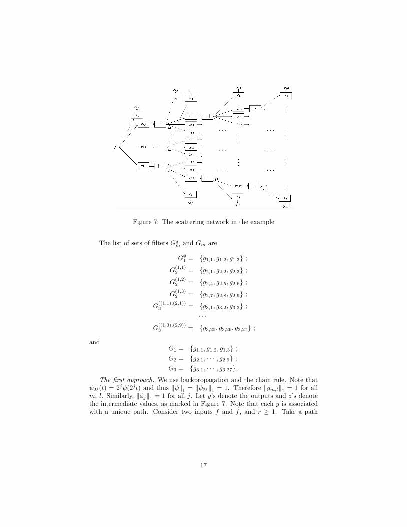
Figure 7: The scattering network in the example

The list of sets of filters Gqm and Gm are

G∅1 = {g1,1, g1,2, g1,3} ;

G(1,1)2 = {g2,1, g2,2, g2,3} ;

G(1,2)2 = {g2,4, g2,5, g2,6} ;

G(1,3)2 = {g2,7, g2,8, g2,9} ;

G((1,1),(2,1))3 = {g3,1, g3,2, g3,3} ;

· · ·

G((1,3),(2,9))3 = {g3,25, g3,26, g3,27} ;

andG1 = {g1,1, g1,2, g1,3} ;

G2 = {g2,1, · · · , g2,9} ;

G3 = {g3,1, · · · , g3,27} .

The first approach. We use backpropagation and the chain rule. Note thatψ2j (t) = 2jψ(2jt) and thus ‖ψ‖1 = ‖ψ2j‖1 = 1. Therefore ‖gm,l‖1 = 1 for allm, l. Similarly, ‖φj‖1 = 1 for all j. Let y’s denote the outputs and z’s denotethe intermediate values, as marked in Figure 7. Note that each y is associatedwith a unique path. Consider two inputs f and f , and r ≥ 1. Take a path

17

q = ((1, l1), (2, l2), (3, l3)) we have

‖y4,l3 − y4,l3‖r = ‖(z3,l3 − z3,l3) ∗ φ4‖r ≤ ‖z3,l3 − z3,l3‖r ‖φ4‖1 = ‖z3,l3 − z3,l3‖r ;

‖z3,l3 − z3,l3‖r = ‖|z2,l2 ∗ g3,l3 | − |z2,l2 ∗ g3,l3 |‖r ≤‖z2,l2 − z2,l2‖r ‖g3,l3‖1 = ‖z2,l2 − z2,l2‖r ;

‖z2,l2 − z2,l2‖r = ‖|z1,l1 ∗ g2,l2 | − |z1,l1 ∗ g2,l2 |‖r ≤‖z1,l1 − z1,l1‖r ‖g2,l2‖1 = ‖z1,l1 − z1,l1‖r ;

‖z1,l1 − z1,l3‖r =∥∥∥|f ∗ g1,l1 | − ∣∣∣f ∗ g1,l1 ∣∣∣∥∥∥

r≤∥∥∥f − f∥∥∥

r‖g1,l1‖1 =

∥∥∥f − f∥∥∥r.

and similarly for all output ym,lm ’s. Therefore, we have

|||Φ(f)− Φ(f)|||2 =∑m,lm

‖ym,lm − ym,lm‖22 ≤ 40

∥∥∥f − f∥∥∥22.

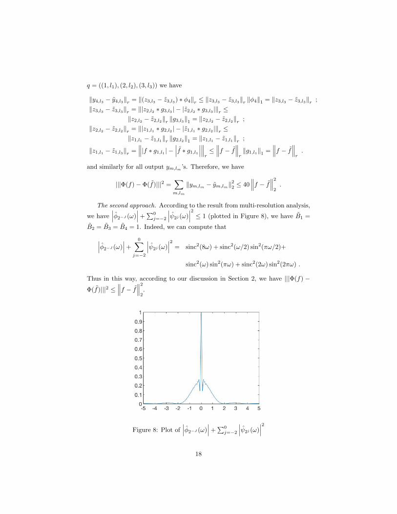
The second approach. According to the result from multi-resolution analysis,

we have∣∣∣φ2−J (ω)

∣∣∣+∑0j=−2

∣∣∣ψ2j (ω)∣∣∣2 ≤ 1 (plotted in Figure 8), we have B1 =

B2 = B3 = B4 = 1. Indeed, we can compute that

∣∣∣φ2−J (ω)∣∣∣+

0∑j=−2

∣∣∣ψ2j (ω)∣∣∣2 = sinc2(8ω) + sinc2(ω/2) sin2(πω/2)+

sinc2(ω) sin2(πω) + sinc2(2ω) sin2(2πω) .

Thus in this way, according to our discussion in Section 2, we have |||Φ(f) −Φ(f)|||2 ≤

∥∥∥f − f∥∥∥22.

Figure 8: Plot of∣∣∣φ2−J (ω)

∣∣∣+∑0j=−2

∣∣∣ψ2j (ω)∣∣∣2

18

The third approach. A lower bound is derived by considering only the outputy1,1 from the input layer. Obviously

|||Φ(f)− Φ(f)|||2 ≥∥∥∥(f − f) ∗ φ1

∥∥∥21.

Thus

supf 6=f

|||Φ(f)− Φ(f)|||2∥∥∥f − f∥∥∥22

≥ supf 6=f

∥∥∥(f − f) ∗ φ1∥∥∥21∥∥∥f − f∥∥∥2

2

=∥∥∥φ1∥∥∥2

∞= 1 .

Therefore, 1 is the exact Lipschitz bound (and Lipschitz constant) in our exam-ple.

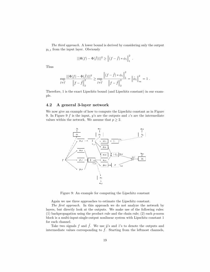
4.2 A general 3-layer network

We now give an example of how to compute the Lipschitz constant as in Figure9. In Figure 9 f is the input, y’s are the outputs and z’s are the intermediatevalues within the network. We assume that p ≥ 2.

Figure 9: An example for computing the Lipschitz constant

Again we use three approaches to estimate the Lipschitz constant.The first approach. In this approach we do not analyze the network by

layers, but directly look at the outputs. We make use of the following rules:(1) backpropagation using the product rule and the chain rule; (2) each p-normblock is a multi-input-single-output nonlinear system with Lipschitz constant 1for each channel.

Take two signals f and f . We use y’s and z’s to denote the outputs andintermediate values corresponding to f . Starting from the leftmost channels,

19

we have for the first layer that

|y1 − y1| =∣∣∣(f − f) ∗ φ1

∣∣∣ ,and thus for any 1 ≤ r ≤ ∞,

‖y1 − y1‖r ≤∥∥∥f − f∥∥∥

r‖φ1‖1 . (4.1)

For the second layer we have

|y2,1 − y2,1| = |(z1,1 − z1,1) ∗ φ2,2| ,

and thus‖y2,1 − y2,1‖r ≤ ‖z1,1 − z1,1‖r ‖φ2‖1 .

With‖z1,1 − z1,1‖r ≤

∥∥∥f − f∥∥∥r‖g1,1‖1 ,

we have‖y2,1 − y2,1‖r ≤

∥∥∥f − f∥∥∥r‖g1,1‖1 ‖φ2‖1 . (4.2)

Similarly,‖y2,2 − y2,2‖r ≤ ‖z1,2 − z1,2‖r ‖φ2‖1 ,

and with

|z1,2 − z1,2| =∣∣∣ (|f ∗ g1,2|p + |f ∗ g1,3|p + |f ∗ g1,4|p)

1/p−(∣∣∣f ∗ g1,2∣∣∣p +∣∣∣f ∗ g1,3∣∣∣p +

∣∣∣f ∗ g1,4∣∣∣p)1/p ∣∣∣≤(∣∣∣(f − f) ∗ g1,2

∣∣∣p +∣∣∣(f − f) ∗ g1,3

∣∣∣p +∣∣∣(f − f) ∗ g1,4

∣∣∣p)1/p≤∣∣∣(f − f) ∗ g1,2

∣∣∣+∣∣∣(f − f) ∗ g1,3

∣∣∣+∣∣∣(f − f) ∗ g1,4

∣∣∣we have

‖z1,2 − z1,2‖r ≤∥∥∥f − f∥∥∥ (‖g1,2‖1 + ‖g1,3‖1 + ‖g1,4‖1) .

Therefore

‖y2,2 − y2,2‖r ≤∥∥∥f − f∥∥∥ (‖g1,2‖1 + ‖g1,3‖1 + ‖g1,4‖1) ‖φ2‖1 . (4.3)

For the third layer we have

‖y3,1 − y3,1‖r ≤ ‖z2,1 − z2,1‖r ‖φ3‖1 .

With‖z2,1 − z2,1‖r ≤ ‖z1,1 − z1,1‖r ‖g2,1‖1 ,

20

we have‖y3,1 − y3,1‖r ≤

∥∥∥f − f∥∥∥r‖g1,1‖1 ‖g2,1‖1 ‖φ3‖1 . (4.4)

Also,

|z2,2 − z2,2| =∣∣∣ (|z1,1 ∗ g2,2|p + |z1,1 ∗ g2,3|p + |z1,2 ∗ g2,4|p)

1/p−

(|z1,1 ∗ g2,2|p + |z1,1 ∗ g2,3|p + |z1,2 ∗ g2,4|p)1/p∣∣∣

≤ (|(z1,1 − z1,1) ∗ g2,2|p + |(z1,1 − z1,1) ∗ g2,3|p +

|(z1,2 − z1,2) ∗ g2,4|p)1/p

≤ |(z1,1 − z1,1) ∗ g2,2|+ |(z1,1 − z1,1) ∗ g2,3|+ |(z1,2 − z1,2) ∗ g2,4| ,

which gives

‖z2,2 − z2,2‖r ≤ ‖z1,1 − z1,1‖r (‖g2,2‖1 + ‖g2,3‖1) + ‖z1,2 − z1,2‖r ‖g2,4‖1 .

A more obvious relation is

‖z2,3 − z2,3‖r ≤ ‖z1,2 − z1,2‖r ‖g2,5‖1 .

Under conditions in Theorem 3.3, we have

‖z2,4 − z2,4‖r = ‖z2,3z2,2 − z2,3z2,2‖r= ‖z2,3z2,2 − z2,3z2,2 + z2,3z2,2 − z2,3z2,2‖r≤ ‖z2,3 − z2,3‖r ‖z2,2‖∞ + ‖z2,3‖∞ ‖z2,2 − z2,2‖r≤ ‖z2,2 − z2,2‖r + ‖z2,3 − z2,3‖r ,

and consequently we have

‖y3,2 − y3,2‖r ≤ ‖z2,4 − z2,4‖r ‖φ3‖1≤ (‖z2,2 − z2,2‖r + ‖z2,3 − z2,3‖r) ‖φ3‖1≤ ‖z1,1 − z1,1‖r (‖g2,2‖1 + ‖g2,3‖1) ‖φ3‖1 +

‖z1,2 − z1,2‖r (‖g2,4‖1 + ‖g2,5‖1) ‖φ3‖1≤∥∥∥f − f∥∥∥

r

(‖g1,1‖1 (‖g2,2‖1 + ‖g2,3‖1)+

(‖g1,2‖1 + ‖g1,3‖1 + ‖g1,4‖1)(‖g2,4‖1 + ‖g2,5‖1))‖φ3‖1 .

(4.5)

21

Collecting (4.1)-(4.5) we have∑m,l

‖ym,l − ym,l‖r ≤∥∥∥f − f∥∥∥

r

(‖φ1‖1 + ‖g1,1‖1 ‖φ2‖1 +

(‖g1,2‖1 + ‖g1,3‖1 + ‖g1,4‖1) ‖φ2‖1 +

‖g1,1‖1 ‖g2,1‖1 ‖φ3‖1 +(‖g1,1‖1 (‖g2,2‖1 + ‖g2,3‖1)+

(‖g1,2‖1 + ‖g1,3‖1 + ‖g1,4‖1)(‖g2,4‖1 + ‖g2,5‖1))‖φ3‖1

)=∥∥∥f − f∥∥∥

r

(‖φ1‖1 + (‖g1,1‖1 + ‖g1,2‖1 + ‖g1,3‖1 + ‖g1,4‖1)

‖φ2‖1 +(‖g1,1‖1 (‖g2,1‖1 + ‖g2,2‖1 + ‖g2,3‖1)+

(‖g1,2‖1 + ‖g1,3‖1 + ‖g1,4‖1)(‖g2,4‖1 + ‖g2,5‖1))‖φ3‖1

).

On the other hand we also have

|||Φ(f)− Φ(f)|||2 =∑m,l

‖ym,l − ym,l‖22

≤∥∥∥f − f∥∥∥2

2

(‖φ1‖21 + ‖g1,1‖21 ‖φ2‖

21 +

(‖g1,2‖1 + ‖g1,3‖1 + ‖g1,4‖1)2 ‖φ2‖21 +

‖g1,1‖21 ‖g2,1‖21 ‖φ3‖

21 +

(‖g1,1‖1 (‖g2,2‖1 + ‖g2,3‖1)+

(‖g1,2‖1 + ‖g1,3‖1 + ‖g1,4‖1)(‖g2,4‖1 + ‖g2,5‖1))2‖φ3‖21

).

(4.6)The second approach. To apply our formula, we first add δ’s and form

a network as in Figure 10. We have a three-layer network and as we havediscussed, we can compute, since p ≥ 2, that

B1 =

∥∥∥∥|g1,1|2 + |g1,2|2 + |g1,3|2 + |g1,4|2 +∣∣∣φ1∣∣∣2∥∥∥∥

∞;

B2 = max

{1,

∥∥∥∥|g2,1|2 + |g2,2|2 + |g2,3|2 +∣∣∣φ2∣∣∣2∥∥∥∥

∞,

∥∥∥∥|g2,4|2 + |g2,5|2 +∣∣∣φ2∣∣∣2∥∥∥∥

∞

};

B3 = max

{2,∥∥∥φ3∥∥∥2

∞

};

B4 = max

{1,∥∥∥φ3∥∥∥2

∞

}.

Then the Lipschitz constant is given by (B1B2B3B4)1/2, that is,

|||Φ(f)− Φ(f)|||2 ≤ (B1B2B3B4)∥∥∥f − f∥∥∥2

2. (4.7)

22

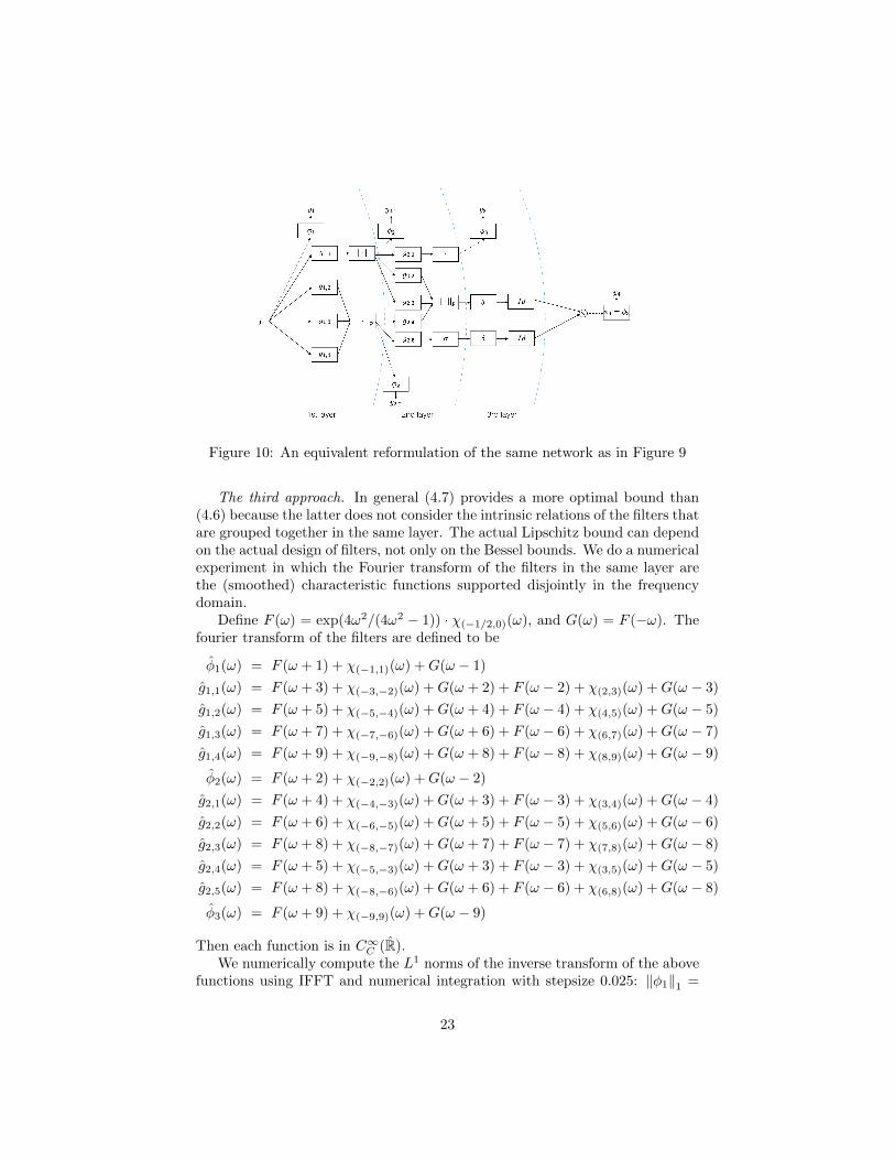
Figure 10: An equivalent reformulation of the same network as in Figure 9

The third approach. In general (4.7) provides a more optimal bound than(4.6) because the latter does not consider the intrinsic relations of the filters thatare grouped together in the same layer. The actual Lipschitz bound can dependon the actual design of filters, not only on the Bessel bounds. We do a numericalexperiment in which the Fourier transform of the filters in the same layer arethe (smoothed) characteristic functions supported disjointly in the frequencydomain.

Define F (ω) = exp(4ω2/(4ω2 − 1)) · χ(−1/2,0)(ω), and G(ω) = F (−ω). Thefourier transform of the filters are defined to be

φ1(ω) = F (ω + 1) + χ(−1,1)(ω) +G(ω − 1)

g1,1(ω) = F (ω + 3) + χ(−3,−2)(ω) +G(ω + 2) + F (ω − 2) + χ(2,3)(ω) +G(ω − 3)

g1,2(ω) = F (ω + 5) + χ(−5,−4)(ω) +G(ω + 4) + F (ω − 4) + χ(4,5)(ω) +G(ω − 5)

g1,3(ω) = F (ω + 7) + χ(−7,−6)(ω) +G(ω + 6) + F (ω − 6) + χ(6,7)(ω) +G(ω − 7)

g1,4(ω) = F (ω + 9) + χ(−9,−8)(ω) +G(ω + 8) + F (ω − 8) + χ(8,9)(ω) +G(ω − 9)

φ2(ω) = F (ω + 2) + χ(−2,2)(ω) +G(ω − 2)

g2,1(ω) = F (ω + 4) + χ(−4,−3)(ω) +G(ω + 3) + F (ω − 3) + χ(3,4)(ω) +G(ω − 4)

g2,2(ω) = F (ω + 6) + χ(−6,−5)(ω) +G(ω + 5) + F (ω − 5) + χ(5,6)(ω) +G(ω − 6)

g2,3(ω) = F (ω + 8) + χ(−8,−7)(ω) +G(ω + 7) + F (ω − 7) + χ(7,8)(ω) +G(ω − 8)

g2,4(ω) = F (ω + 5) + χ(−5,−3)(ω) +G(ω + 3) + F (ω − 3) + χ(3,5)(ω) +G(ω − 5)

g2,5(ω) = F (ω + 8) + χ(−8,−6)(ω) +G(ω + 6) + F (ω − 6) + χ(6,8)(ω) +G(ω − 8)

φ3(ω) = F (ω + 9) + χ(−9,9)(ω) +G(ω − 9)

Then each function is in C∞C (R).We numerically compute the L1 norms of the inverse transform of the above

functions using IFFT and numerical integration with stepsize 0.025: ‖φ1‖1 =

23

1.8265, ‖g1,1‖1 = 2.0781, ‖g1,2‖1 = 2.0808, ‖g1,3‖1 = 2.0518, ‖g1,4‖1 = 2.0720,‖φ2‖1 = 2.0572, ‖g2,1‖1 = 2.0784, ‖g2,2‖1 = 2.0734, ‖g2,3‖1 = 2.0889, ‖g2,4‖1 =2.2390, ‖g2,5‖1 = 2.3175, ‖φ3‖1 = 2.6378. Then the constant on the right-handside of Inequality (4.6) is 966.26, and by taking the square root we get theLipschitz bound computed using the first approach is equal to Γ1 = 98.3.

It is no effort to conclude that in the second approach, B1 = B2 = B4 = 1and B3 = 2. Therefore the Lipschitz bound computed using the second approachis Γ2 =

√2. Note that in this example the conditions in Lemma 3.5 is satisfied.

The experiment suggests that the Lipschitz bound associated with our set-ting of filters is Γ3 = 1.1937. We numerically compute the output of the networkand record the largest ratio |||Φ(f) − Φ(f)|||/||f − f ||2 over one million itera-tions. Numerically, we consider the range [−20, 20] for both the time domainand the frequency domain and take stepsize to be 0.025. For each iteration wegenerate two randomly signals on [−20, 20] with stepsize 1 and then upsampleto the same scale with stepsize 0.025.

We conclude that the naıve first approach may lead to a much larger Lip-schitz bound for analysis, and the second approach gives a more reasonableestimation.

Acknowledgments

The first author was partially supported by NSF Grant DMS-1413249 and AROGrant W911NF-16-1-0008. The third author was partially supported by NSFGrant DMS-1413249.

References

[1] J. Bruna and S. Mallat, Invariant scattering convolution networks, IEEETransactions on Pattern Analysis and Machine Intelligence 35 (2013), no. 8,1872–1886.

[2] Joan Bruna, Soumith Chintala, Yann LeCun, Serkan Piantino, ArthurSzlam, and Mark Tygert, A theoretical argument for complex-valued con-volutional networks, CoRR abs/1503.03438 (2015).

[3] Sepp Hochreiter and Jurgen Schmidhuber, Long short-term memory, Neu-ral Comput. 9 (1997), no. 8, 1735–1780.

[4] Yoshua Bengio Ian Goodfellow and Aaron Courville, Deep learning, Bookin preparation for MIT Press, 2016.

[5] Yann Lecun, Yoshua Bengio, and Geoffrey Hinton, Deep learning, Nature521 (2015), no. 7553, 436–444.

24

[6] Roi Livni, Shai Shalev-shwartz, and Ohad Shamir, On the computationalefficiency of training neural networks, Advances in Neural Information Pro-cessing Systems 27 (Z. Ghahramani, M. Welling, C. Cortes, N.d. Lawrence,and K.q. Weinberger, eds.), Curran Associates, Inc., 2014, pp. 855–863.

[7] Stphane Mallat, Group invariant scattering, Communications on Pure andApplied Mathematics 65 (2012), no. 10, 1331–1398.

[8] Tara N. Sainath, Oriol Vinyals, Andrew W. Senior, and Hasim Sak, Con-volutional, long short-term memory, fully connected deep neural networks,2015 IEEE International Conference on Acoustics, Speech and Signal Pro-cessing, ICASSP 2015, South Brisbane, Queensland, Australia, April 19-24,2015, 2015, pp. 4580–4584.

[9] Christian Szegedy, Wei Liu, Yangqing Jia, Pierre Sermanet, Scott Reed,Dragomir Anguelov, Dumitru Erhan, Vincent Vanhoucke, and Andrew Ra-binovich, Going deeper with convolutions, CVPR 2015, 2015.

[10] Christian Szegedy, Wojciech Zaremba, Ilya Sutskever, Joan Bruna, Du-mitru Erhan, Ian J. Goodfellow, and Rob Fergus, Intriguing properties ofneural networks, CoRR abs/1312.6199 (2013).

[11] Thomas Wiatowski and Helmut Bolcskei, Deep convolutional neural net-works based on semi-discrete frames, Proc. of IEEE International Sympo-sium on Information Theory (ISIT), June 2015, pp. 1212–1216.

[12] , A mathematical theory of deep convolutional neural networks forfeature extraction, IEEE Transactions on Information Theory (2015).

25