Embed Size (px)
Citation preview

Public PROCEDURES
Study Process and Methodology Manual:Estimating Economically Optimum and Market
Equilibrium Reserve Margins (EORM and MERM) Version 1.0
ERCOT Public 12/11/2017

EORM/MERM Study Process and Methodology Manual ERCOT Public
Document Revisions
Date Version Description Author(s)11/03/2017 0.1 Initial draft, intended for public
commentsPeter Warnken, ERCOTJulie Jin, ERCOTNick Wintermantel, Astrape ConsultingKevin Carden, Astrape ConsultingKathleen Spees, The Brattle GroupRoger Lueken, The Brattle Group
12/12/2017 1.0 Final version Edits by Peter Warnken, ERCOT, based on stakeholder comments
© 2017 Electric Reliability Council of Texas, Inc. All rights reserved.

EORM/MERM Study Process and Methodology Manual ERCOT Public
Sign-OffTitle: Manager, Resource Adequacy
Name: Peter Warnken
Date: 12/12/2017
© 2017 Electric Reliability Council of Texas, Inc. All rights reserved.

EORM/MERM Study Process and Methodology Manual ERCOT Public
Table of Contents
1. Introduction.........................................................................................................................1
2. Study Development Process..............................................................................................1
2.1. Project Team................................................................................................................2
2.2. Selection of a Simulation Year.....................................................................................2
2.3. Study Development Timeline........................................................................................2
2.4. Public Stakeholder Process..........................................................................................3
2.4.1. Sensitivity Analysis.............................................................................................3
2.4.2. Scenario Analysis...............................................................................................4
2.5. In-Scope and Out-of-Scope Analyses..........................................................................4
2.6. Report Format and Distribution....................................................................................4
3. Required Modeling and Software Capabilities....................................................................5
4. Load Modeling....................................................................................................................5
4.1. Peak and Energy Forecasts.........................................................................................5
4.2. Weather Uncertainty Modeling.....................................................................................6
4.3. Non-weather Load Uncertainty Modeling.....................................................................6
5. Supply Resource Modeling.................................................................................................7
5.1. Supply Mix....................................................................................................................8
5.1.1. Baseline Resource Mix......................................................................................8
5.1.2. Simulation of Different Reserve Margin Levels..................................................8
5.2. Supply Resource Characteristics.................................................................................8
5.2.1. Thermal Resources............................................................................................8
5.2.2. Marginal Resource Technologies.......................................................................9
5.2.3. Thermal Unit Availability and Outage Modeling...............................................10
5.2.4. Private Use Network Resources......................................................................12
5.2.5. Switchable Generation Resources...................................................................13
5.2.6. Wind Resources...............................................................................................13
5.2.7. Solar Resources...............................................................................................14
5.2.8. Hydroelectric Resources..................................................................................15
5.2.9. Distributed Energy Resources.........................................................................16
5.2.10. Energy Storage Technologies..........................................................................16
5.3. Fuel Prices..................................................................................................................17
6. Demand-Side Resource Modeling....................................................................................17
© 2017 Electric Reliability Council of Texas, Inc. All rights reserved.
EORM/MERM Study Process and Methodology Manual ERCOT Public
6.1. Dispatchable Resources.............................................................................................17
6.2. Non-dispatchable Resources.....................................................................................19
6.3. Energy Efficiency........................................................................................................20
7. Transmission System Modeling........................................................................................20
7.1. Transmission Topology..............................................................................................20
7.1.1. Transmission Intertie Availability......................................................................21
7.1.2. Import/Export Mechanics during Scarcity Conditions......................................21
8. Representation of ERCOT Markets..................................................................................21
8.1. Energy and Ancillary Service Markets........................................................................21
8.2. Scarcity Conditions.....................................................................................................21
8.2.1. Administrative Market Parameters...................................................................22
8.2.2. Emergency Procedures and Marginal Costs...................................................22
8.2.3. Emergency Generation....................................................................................23
8.2.4. Operating Reserve Demand Curve..................................................................24
8.2.5. Power Balance Penalty Curve.........................................................................25
8.3. Generator Cost of New Entry (CONE).......................................................................26
8.4. Value of Lost Load (VOLL).........................................................................................27
9. Study Results....................................................................................................................27
9.1. Reserve Margin Accounting.......................................................................................27
9.2. Total System Cost and Energy Margin.......................................................................28
9.3. Economically Optimal Reserve Margin......................................................................30
9.4. Market Equilibrium Reserve Margin...........................................................................30
9.5. EORM and MERM Uncertainty Analysis....................................................................30
9.6. Physical System Reliability Standards.......................................................................30
9.7. Reporting a Reference Reserve Margin Level for NERC Reliability Assessments....31
9.7.1. Background on NERC’s Reference Margin Level............................................31
9.7.2. Use of the Reference Margin Level in NERC Reliability Assessments...........32
9.7.3. Reporting a Reference Margin Level to NERC................................................32
10. Appendices.......................................................................................................................33
10.1. Filed Letter to the PUCT on Conducting EORM/MERM Studies...............................33
10.2. Calculation of Probability Weights for Weather-year Load Forecasts........................35
10.2.1. Weather-risk Index...........................................................................................35
10.2.2. Outlier Thresholds............................................................................................36
10.2.3. Frequency Histogram.......................................................................................37
© 2017 Electric Reliability Council of Texas, Inc. All rights reserved.
EORM/MERM Study Process and Methodology Manual ERCOT Public
10.2.4. Identify Index Risk Ranges..............................................................................38
10.2.5. Assigning Probabilities to the Risk Categories................................................39
10.2.6. Assigning Probabilities to the Weather Years..................................................40
10.3. Incorporation of Stakeholder Comments in the Draft Manual....................................42
10.3.1. Modeling of Price Responsive Demand (PRD)................................................42
10.3.2. NERC Reference Reserve Margin Level.........................................................42
10.3.3. Resource Costs................................................................................................42
10.4. List of Acronyms.........................................................................................................42
Table of Figures
Figure 1: Indicative RM Study Schedule..............................................................................................3Figure 2: Non-Weather Forecast Uncertainty with Increasing Forward Period....................................7Figure 3: Three-Year Forward LFE with Discrete Error Points Modeled.............................................7Figure 4: Aggregate Wind Profiles based on 13 Historical Weather Years (2002-2014)....................14Figure 5: Seasonal Average Daily Solar Profiles................................................................................15Figure 6: Regression Equation Determined for Modeling Hydro Peak-Shaving Capacity..................16Figure 7: Operating Reserve Demand Curves (2014 Study).............................................................25Figure 8: Power Balance Penalty Curve (2014 Study).......................................................................26Figure 9: Sample Chart Showing Weighted Average Total System Cost by Reserve Margin...........29Figure 10: Sample Chart Showing Weighted Average Energy Margin by Reserve Margin...............29Figure 11: Tornado Diagram for EORM Sensitivities.........................................................................30Figure 12: NERC Reference Margin Level Definition and Reporting Instructions..............................31Figure 13: Weather Risk Index Values, 1980-2016............................................................................36Figure 14: Weather-Risk Index Histogram..........................................................................................38
Table of Tables
Table 1: SERVM Thermal Resource Variables....................................................................................8Table 2: Gas-fired Resource Mix, Interconnection Request Projects...................................................9Table 3: NERC GADS Event Types....................................................................................................10Table 4: Supply Curves for Private Use Network Generation Resources...........................................12Table 5: Call Limits for Demand Response Programs.......................................................................18Table 6: SERVM Demand-Response Variables................................................................................18Table 7: ERCOT Scarcity Pricing Parameters Assumed for 2016 (2014 RM Study)........................22Table 8: Emergency Procedures and Marginal Costs (2014 RM Study)...........................................23Table 9: Gross Cost of New Entry (2014 Study)................................................................................27Table 10: Consecutive Days of Temperatures exceeding 100 Degrees for 1980.............................35Table 11: Calculation of Weather Risk Index Values for 1980 and 1987...........................................36Table 12: Quartile Fence Parameters................................................................................................37Table 13: Weather-Risk Index Frequencies and Relative Frequency Percentages..........................37Table 14: Categorization of Index Values by Risk Level....................................................................39Table 15: Distance Ratio Calculations...............................................................................................40Table 16: Weather-Year Probability Assignment by Risk Category...................................................40Table 17: Derivation of Weather-Year Probabilities...........................................................................41
© 2017 Electric Reliability Council of Texas, Inc. All rights reserved.
EORM/MERM Study Process and Methodology Manual ERCOT Public
1. Introduction
This manual outlines the process and methodologies for estimating the Economically Optimum Reserve Margin (EORM) and Market Equilibrium Reserve Margin (MERM) for the ERCOT Region (the “RM Study”). The manual was developed after receiving feedback on proposed methodologies and study management topics presented at a public workshop held on April 14, 2017, a follow-up public conference call held on May 23, 20171, and subsequent comments received by email. The manual will be updated as needed to reflect significant market events, changes in market design characteristics, and modifications to the study scope or requirements.
The genesis of the manual stems from a high-level plan for determining these Reserve Margin values going forward. The plan was proposed to the Public Utility Commission of Texas (PUCT) and memorialized in a filed letter to the PUCT in October 2016. The plan was subsequently accepted by the Commission. The ERCOT letter is provided as Appendix 10.1.
Many of the methodologies outlined in this manual were originally implemented for an EORM/MERM study conducted for the Commission by the Brattle Group and Astrapé Consulting in late 2013. The manual was thus written with the help of these two consulting companies. Details on the Commission’s Reserve Margin study can be found in the report, Estimating the Economically Optimal Reserve Margin in ERCOT (January 31, 2014).2 This study will hereafter be referred to as the “2014 RM Study”.
This manual constitutes the following main sections:
The study development process Required modeling and software capabilities for conducting the study Modeling of forecasted loads and forecast uncertainty Supply resource modeling Fuel prices Demand-side resource modeling Transmission system modeling ERCOT market representation Study results Appendices
o ERCOT letter to the PUCT regarding an RM Study work plano Calculation of Probability Weights for Weather-year Load Forecastso Responses to Stakeholder on the draft manualo List of Acronyms
2. Study Development Process
This section covers (1) make-up of the project team, (2) the approach for planning, developing and reporting the RM Study, (3) the anticipated project schedule, (4) public stakeholder participation, and (5) the scope of RM Study activities.
1 Workshop documentation is available at: http://www.ercot.com/calendar/2017/4/14/117459. Conference call documentation is available at: http://www.ercot.com/calendar/2017/5/23/122934.2 http://www.ercot.com/content/wcm/lists/114801/Estimating_the_Economically_Optimal_Reserve_Margin_in_ERCOT_Revised.pdf
© 2017 Electric Reliability of Texas, Inc. All rights reserved. 1

EORM/MERM Study Process and Methodology Manual ERCOT Public
2.1. Project Team
The RM Study will be a multi-departmental effort with staff participation from the following ERCOT departments:
Resource Adequacy Wholesale Market Design & Operations Load Forecasting and Analysis
System modeling will be conducted by an independent partyspecifically a consultant team with extensive experience in conducting resource adequacy studies and operating software that meets the requirements outlined in Section 3. ERCOT staff will provide model data and work with the consultant team on any analyses needed to support the RM Study; for example, the development of probabilistic supply curves for price-responsive supply- and demand-side resources.
2.2. Selection of a Simulation Year
The RM Study is conducted for a single simulation year, specified as the fourth year beyond the year during which the Study is conducted. For example, the RM Study conducted in 2018 would simulate the year 2022. Simulating the fourth future year is intended to reflect the end of a sufficient planning period for resource developers that have submitted interconnection requests for proposed projects. The planning period accounts for the lead-time needed to finalize investment decisions and construct generation resources.
2.3. Study Development Timeline
The RM Study is conducted every even-numbered year, starting with 2018. Table 1 shows the timeline for study activities3, which commence in the second half of the RM Study off-year and ends with the posting of the RM Study report in mid-November of the RM Study year. The RM Study schedule is intended to generally align with the loss-of-load modeling activities that support the North American Electric Reliability Corporation (NERC) biennial Probabilistic Assessment.4 Since the RM Study and NERC Probabilistic Assessment use the same modeling framework and most of the same data, this alignment reduces combined study costs and helps ensure consistency in probabilistic modeling methods and data used for the two studies.
Figure 1: Indicative RM Study Schedule
3 The activity timelines shown are indicative, and will be adjusted based on the agreed-to Study Plan. For the inaugural 2018 RM Study, the Study Plan is anticipated to be finalized in the first quarter of 2018.4 The main purpose of the Probabilistic Assessment is to derive a common set of monthly and annual probabilistic reliability metrics (e.g., Loss of Load Hours (LOLH and Expected Unserved Energy (EUE)) across the NERC footprint for two future years. It is not meant to determine a Reserve Margin target or evaluate different Reserve Margin levels. For more background on the NERC Probabilistic Assessment, see the NERC 2016 Probabilistic Assessment report (March 2017), available at: http://www.nerc.com/pa/RAPA/ra/Reliability%20Assessments%20DL/2016ProbA_Report_Final_March.pdf.
© 2017 Electric Reliability of Texas, Inc. All rights reserved. 2
Study YearQ3 Q4 Jan Feb Apr May Oct Dec
Public Stakeholder Process (Pre-study) Develop Study Plan to Reflect Methodology Updates SAWG Methodology Review Meetings, as needed X X Study Plan presentation at SAWG, WMS, TAC as needed X X X Finalize Study Plan X Study Preparation Develop updated/new model inputs Update Model DatabaseConduct EORM/MERM Study Conduct base simulations Conduct sensitivity simulations Report DevelopmentPublic Stakeholder Process (Post-study completion) Report Review/Comment (PUCT, ERCOT Forums) Complete Final Report and Post
NERC Probabilistic Reliability Assessment modeling
Jul SepJunMarStudy Off-Year
NovAug

EORM/MERM Study Process and Methodology Manual ERCOT Public
2.4. Public Stakeholder Process
As indicated in the RM Study Schedule, each RM Study cycle will have public involvement during the study planning phase and for review and comment of the RM Study draft report.
During the study cycle off-year (currently the odd-numbered years), ERCOT will facilitate RM Study planning discussions during at least two monthly Supply Analysis Working Group (SAWG) meetings. The discussions will be scheduled for the third quarter at the direction of the SAWG Chair. The goals of the SAWG planning discussions are three-fold:
1. Identify the need for methodology updates (in which case this Manual will be updated by year-end pending agreement on the proposed changes). Changes may include, but not be limited to, CDR-related Protocol revisions, market-design-related Protocol/Binding Document revisions, and the source and derivation of model inputs (not the inputs themselves).
2. Propose and discuss the Study Plan. The Study Plan will lay out the actual project schedule and describe any methodology updates.
3. Discuss proposals for sensitivity/scenario analyses as described below, and add them as potential work items to the Study Plan based on SAWG member recommendations.
Based on SAWG member comments, the Study Plan will be revised and presented at a Wholesale Market Subcommittee (WMS) meeting. The Study Plan may also be presented at a Technical Advisory Committee (TAC) meeting as directed by the WMS. ERCOT expects the final Study Plan to be completed by the end of the RM Study off-year. The final Study Plan will be posted to the ERCOT Resource Adequacy Webpage on www.ercot.com.
ERCOT anticipates preparing the RM Study Report during August and September of the Study Year. A public draft of the Report will be posted to the Resource Adequacy Webpage, and a Market Notice will be issued announcing the availability of the report for review and comment. The comment period will be six weeks, and may be adjusted as needed. Presentations on the report before various ERCOT Market Participant forums will be scheduled during the comment period.
2.4.1. Sensitivity Analysis
Sensitivity analysis is defined as changing a single key model input variable or parameter to determine how the change affects the simulation outcome (system cost, EORM/MERM level margin level, or both). In order to develop uncertainty ranges for MERM values, as mentioned in Section 2.5, a number of sensitivity analyses will be conducted as a regular feature of each RM Study. All other proposed sensitivity analyses are considered optional projects.
2.4.2. Scenario Analysis
Scenario analysis constitutes changing multiple model variables and/or parameters to investigate different market outcomes or futures. All proposed scenario analyses are considered optional projects.
2.5. In-Scope and Out-of-Scope Analyses
In-scope analysis for each RM Study consists of the determination of a base-case (or expected) EORM value, a base-case MERM value, and certain sensitivity simulations desired for reporting
© 2017 Electric Reliability of Texas, Inc. All rights reserved. 3

EORM/MERM Study Process and Methodology Manual ERCOT Public
uncertainty ranges for the base-case EORM and MERM values. In-scope analysis is covered in the indicative RM Study Schedule (Figure 1).
Out-of-scope analysis consists of the following:
Sensitivity or scenario analyses intended to help understand policy interventions, trends, or events that reflect a significant change to the RM study’s base-case version of the future.
Other analyses that are considered ancillary to the in-scope study activities.
An example of an out-of-scope analysis is the calculation of Effective Load Carrying Capability (ELCC) for wind or other resource types.5 ELCC values are currently not used in any ERCOT study or work process, and would entail selecting a physical reliability criterion as the basis for the study.
Out-of-scope analysis proposals would be vetted through the ERCOT RM Study stakeholder process, and if approved, would be reflected as a supplemental activity in the Study Plan. Depending on the timing of the analysis request and priority, such analyses will not necessarily be started and completed concurrently with the biennial RM study. Approved out-of-scope analysis proposals can be considered for off-year scheduling with due consideration given to the cost and staff work-load impacts.
2.6. Report Format and Distribution
The RM Study report will have the following main sections:
Executive Summary
Methodology Changes (if there are deviations with respect to the ones documented in the most current version of this Manual)
Key Model Inputs and Parameters
Study Results, including sensitivities for uncertainty analysis (see Section 9)
Appendices
The final RM Study report, as well as updates to this Manual, will be posted to the Resource Adequacy Webpage.
3. Required Modeling and Software Capabilities
Resource adequacy studies require system planners to capture uncertainty distributions of future load, weather, and generator performance. Thousands of model iterations must be simulated for a single year to capture the full distribution of possible outcomes. Because the RM Study captures economic outputs as well as physical reliability metrics, an hourly chronological model with an economic commitment and dispatch of resources to load is required. The following is a list of more detailed modeling requirements for the RM Study:
5 ELCC is a method for calculating the percentage capacity contribution (or credit) of a resource type, and is usually calculated for intermittent renewables resources like wind power. The basic ELCC calculation framework is to run system simulations both with and without the resource, thereby determining the amount of additional conventional thermal capacity required to achieve the same reliability level as determined by a reliability risk target and associated reliability measure (e.g., a Loss-of-Load Event expectation of 0.1 events in one year). The ELCC indicates the resource’s percentage of total nameplate capacity that can be relied upon for system reliability.
© 2017 Electric Reliability of Texas, Inc. All rights reserved. 4
EORM/MERM Study Process and Methodology Manual ERCOT Public
Ability to conduct hourly chronological hourly simulations for an entire year. Economic commitment and dispatch of resources considering physical unit constraints,
including minimum up time, minimum down times, start up times, and ramp rates. Operating Reserve Demand Curve (ORDC) implementation to calculate hourly market prices
paid to generators for energy and ancillary services during all hours of the year, including hours with capacity shortages.
Monte Carlo algorithms to capture the frequency and duration of random full and partial (derated) generator outages.
Ability to incorporate load and weather uncertainty. Ability to simulate emergency operating procedures such as demand response programs,
voltage control, or other unique characteristics of the system. Multi-area modeling allowing energy to be transferred between regions subject to economics
and transmission constraints via a pipe and bubble representation of the system. Sufficient speed to simulate thousands of scenarios for a specific study year. Ability to calculate production costs, hourly market prices, generator revenues, customer
costs, and physical reliability metrics such as Loss of Load Hours (LOLH) and Expected Unserved Energy (EUE) across a range of system reserve margin levels.
4. Load Modeling
This section describes the methodology and data sources for modeling hourly loads for the simulation forecast year, as well as the associated load uncertainty. Load uncertainty is modeled as two separate load forecast error (LFE) components: weather-driven and non-weather-driven. These two uncertainty components are described in Sections 4.2 and 4.3.
4.1. Peak and Energy Forecasts
The RM Study will include the most current ERCOT hourly coincident load forecast for the study year (officially called the “Long-Term Demand and Energy Forecast”). The load forecast is an aggregation of ERCOT’s eight weather zone “normal” forecasts, also referred to as 50th Percentile, P50, or 50/50 forecasts. As mentioned later in this manual, the ERCOT system will be modeled as a single zone rather than multiple weather zones or other geographically-based regions.
The forecast report, which describes the forecasting methodology, assumptions and data sources, is posted to the Long-Term Load Forecast Webpage on www.ercot.com (http://www.ercot.com/gridinfo/load/forecast).
The hourly load forecast shapes reflecting various weather years will be grossed up for price responsive demand as discussed in more detail in Section 6. Since the market price is subject to a number of variables, price-responsive demand impacts will be modeled like supply-side resources in the simulations to capture a range of possible contributions.
4.2. Weather Uncertainty Modeling
Weather is one of the key drivers of loss-of-load hours, and weather uncertainty is a key component of LFE that is modeled for the RM Study. To capture weather uncertainty in the simulations, annual hourly load forecasts based on historical hourly weather conditions going back to 1980 will be entered into the model. For example, an RM Study conducted in 2020 will use 40 hourly load
© 2017 Electric Reliability of Texas, Inc. All rights reserved. 5

EORM/MERM Study Process and Methodology Manual ERCOT Public
forecasts for 2024 based on historical hourly weather conditions for each year of the period 1980-2019.
Note that this number of historical weather-year forecasts for the RM Study is significantly larger than the number of weather-year forecasts used for the official P50 load forecast. Consequently, averaging the peak values of all the simulation-year load forecasts may not equal the official P50 peak value reported in the CDR and other ERCOT public materials.
To represent the weather-year load forecasts as a probabilistic variable in the system simulations, ERCOT must consider the probability of each weather-year occurring in the future. Most important for the probability analysis is identifying outlier (or extreme) weather years and assigning appropriate probability weights that reflect a smaller likelihood of occurrence than those for other years. Due to the strong correlation between high ambient temperatures, high loads, and frequency of loss-of-load events, ERCOT’s outlier analysis focuses on identifying those years marked by consecutive days of extremely high temperatures (greater than or equal to 100 F) experienced by multiple large population centers in the ERCOT Region.
Based on statistical outlier analysis, ERCOT will develop a series of normalized probability weights [0 x% 1] to be applied to the weather-year forecasts. Appendix 10.2 provides details regarding the probability weight development process, along with sample calculations.
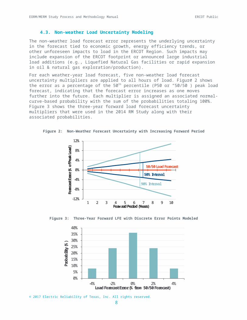
4.3. Non-weather Load Uncertainty Modeling
The non-weather load forecast error represents the underlying uncertainty in the forecast tied to economic growth, energy efficiency trends, or other unforeseen impacts to load in the ERCOT Region. Such impacts may include expansion of the ERCOT footprint or announced large industrial load additions (e.g., Liquefied Natural Gas facilities or rapid expansion in oil & natural gas exploration/production).
For each weather-year load forecast, five non-weather load forecast uncertainty multipliers are applied to all hours of load. Figure 2 shows the error as a percentage of the 50th percentile (P50 or “50/50”) peak load forecast, indicating that the forecast error increases as one moves further into the future. Each multiplier is assigned an associated normal-curve-based probability with the sum of the probabilities totaling 100%. Figure 3 shows the three-year forward load forecast uncertainty multipliers that were used in the 2014 RM Study along with their associated probabilities.
© 2017 Electric Reliability of Texas, Inc. All rights reserved. 6
EORM/MERM Study Process and Methodology Manual ERCOT Public
Figure 2: Non-Weather Forecast Uncertainty with Increasing Forward Period
-12%
-8%
-4%
0%
4%
8%
12%
1 2 3 4 5 6 7 8 9 10
Fore
cast
Err
or (%
of P
eak
Load
)
Forward Period (Years)
50/50 Load Forecast
50% Interval
90% Interval
Figure 3: Three-Year Forward LFE with Discrete Error Points Modeled
0%5%
10%15%20%25%30%35%40%
-4% -2% 0% 2% 4%
Prob
abili
ty (%
)
Load Forecast Error (% from 50/50 Forecast)
To calculate the weighted-average results across all load scenarios, the weather-year probability weights and the non-weather probability weights are multiplied to create joint probability weights.
During the planning phase of each RM Study, ERCOT will determine if non-weather forecast uncertainty multipliers and associated probabilities require updating. ERCOT will then update the multipliers using applicable load and economic growth forecast data. In the 2014 RM Study, the uncertainty was based on historical error in the Congressional Budget Office GDP forecasts. That analysis showed increasing uncertainty with longer forward periods.
5. Supply Resource Modeling
This section discusses the methodologies for modeling conventional thermal resources, intermittent renewable resources, hydroelectric resources, and energy storage resources.
© 2017 Electric Reliability of Texas, Inc. All rights reserved. 7

EORM/MERM Study Process and Methodology Manual ERCOT Public
5.1. Supply Mix
The modeled supply mix consists of the Baseline Resource Mix, along with capacity additions and deductions of specific resource units to establish target Reserve Margin levels for model simulation. These two general resource types are described in the following two sections.
5.1.1. Baseline Resource Mix
The supply-side resource types included in the RM Study constitute conventional thermal (including Private Use Network generators), intermittent renewables, hydro, and energy storage. CDR Reports are used to determine forecast rules for unusual unit types. All resources are modeled based on the seasonal capacities and start/end dates as reported in the mid-year Capacity, Demand, and Reserves (CDR) report. Consistent with CDR development practices, ERCOT will use notices of “Suspension of Operations of a Generation Resource” to specify the availability of units that have been retired, mothballed, or placed on a summer seasonal availability schedule. Mothballed units for which the resource owner reports a seasonal return probability that is equal to or greater than 50% will be available for dispatch for the indicated seasons. Similarly, mothball units for which the seasonal return probability is less than 50% are excluded from the RM Study.
5.1.2. Simulation of Different Reserve Margin Levels
The reserve margin will be lowered from that projected in the mid-year CDR by removing planned generation units. A 6% reserve margin target will be the starting point for the simulations. First, planned gas resources will be removed, and if necessary, planned wind and solar resources will be removed to achieve this starting reserve margin level. The reserve margin will be increased from 6% to 20% by adding the marginal resource as discussed in Section 5.2.2. Simulations will be performed at each incremental level within this range.
5.2. Supply Resource Characteristics
Supply-side resource characteristics incorporated in the RM study are dictated by the specification requirements and options of the production cost model used. The sections below summarize the standard modeled characteristics for the supply-side resource types included in the RM Study.
5.2.1. Thermal Resources
Typically, thermal resources are modeled with maximum capacities by season, minimum capacities, heat rates (most commonly in the form of incremental heat rate curves or block-average values), variable operating and maintenance costs, fuel type, startup costs, hourly startup profiles, hourly shutdown profiles, emission output rate, minimum up-time, minimum down-time, ramp rates, and ancillary service capability. Resources can also be designated as "Must Run" versus economically dispatched. Table 1 shows the primary variables used in SERVM. The ancillary service variables allow users to designate which units can serve regulating reserves and non-spinning reserves. Any resource that has a minimum capacity less than its maximum capacity can provide spinning reserves.
Table 1: SERVM Thermal Resource Variables
Variable Description
capmax maximum capacity that can be input by month or can vary with hourly temperature (MW)
capmin Minimum capacity by month (MW)
© 2017 Electric Reliability of Texas, Inc. All rights reserved. 8
EORM/MERM Study Process and Methodology Manual ERCOT Public
hrcoef Heat rate coefficients (a, b, c)cstvar Variable Operations & Maintenance cost ($/MWh)fuel Fuel type
warm_startup_profile Hourly profile from 0 MW to min outputshutdown_profile Hourly profile from minimum output to 0 MW
emission Emission rates (lb/MMBtu)minimum_uptime Minimum hours online before shutting down
minimum_downtime Minimum hours offline before restartingramp_rate_up Ramp rate up (MW/min)
ramp_rate_down Ramp rate down (MW/min)agc_capable Serve regulation (Yes or No)quickstartunit Serve non-spin (Yes or No)
Thermal resources are committed and dispatched economically while considering all physical constraints of the resources. Thermal resources are dispatched to load and optimized for both energy and ancillary services.
5.2.2. Marginal Resource Technologies
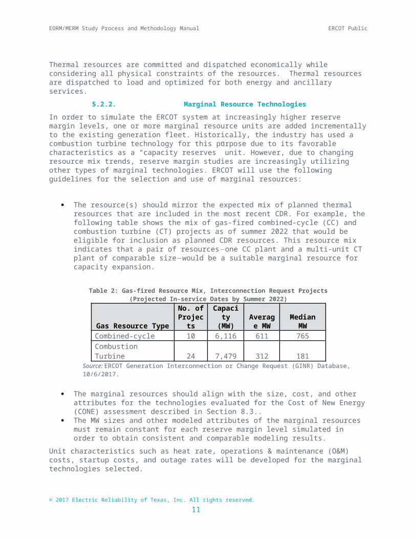
In order to simulate the ERCOT system at increasingly higher reserve margin levels, one or more marginal resource units are added incrementally to the existing generation fleet. Historically, the industry has used a combustion turbine technology for this purpose due to its favorable characteristics as a “capacity reserves” unit. However, due to changing resource mix trends, reserve margin studies are increasingly utilizing other types of marginal technologies. ERCOT will use the following guidelines for the selection and use of marginal resources:
The resource(s) should mirror the expected mix of planned thermal resources that are included in the most recent CDR. For example, the following table shows the mix of gas-fired combined-cycle (CC) and combustion turbine (CT) projects as of summer 2022 that would be eligible for inclusion as planned CDR resources. This resource mix indicates that a pair of resourcesone CC plant and a multi-unit CT plant of comparable sizewould be a suitable marginal resource for capacity expansion.
Table 2: Gas-fired Resource Mix, Interconnection Request Projects(Projected In-service Dates by Summer 2022)
Gas Resource Type
No. of Project
s
Capacity
(MW)Average
MWMedian
MWCombined-cycle 10 6,116 611 765Combustion Turbine 24 7,479 312 181
Source: ERCOT Generation Interconnection or Change Request (GINR) Database, 10/6/2017.
The marginal resources should align with the size, cost, and other attributes for the technologies evaluated for the Cost of New Energy (CONE) assessment described in Section 8.3.
© 2017 Electric Reliability of Texas, Inc. All rights reserved. 9

EORM/MERM Study Process and Methodology Manual ERCOT Public
The MW sizes and other modeled attributes of the marginal resources must remain constant for each reserve margin level simulated in order to obtain consistent and comparable modeling results.
Unit characteristics such as heat rate, operations & maintenance (O&M) costs, startup costs, and outage rates will be developed for the marginal technologies selected.
5.2.3. Thermal Unit Availability and Outage Modeling
The RM Study requires Monte Carlo (MC) simulation of generator forced outages in order to capture the probabilistic nature of such outages. Such modeling requires unit-specific historical time-to-fail distributions, and either time-to-repair distributions or forced outage rates.6 ERCOT also favors models that can represent probabilistic forced outage behavior for both full and partial (derated capacity) outages. The Monte Carlo algorithm performs random sampling of these distributions to create a unit-level outage scenario for each iteration of the simulation. Capacity derate percentages with respect to available MW capacity are also input into the model to create the partial outage distributions.
To determine seasonal historical time-to-fail and time-to-repair distributions for each generation unit, ERCOT will request that thermal generation owners provide an extract of their outage event data from NERC’s Generating Availability Data System (GADS) for an initial three-year historical period, and then provide an extract for an historical two-year period for subsequent RM Studies. The requested GADS extract will include event start and end dates for each unit, as well as the event type. Table 3 shows the GADS event types.
Table 3: NERC GADS Event TypesEvent Code Event Type Description
D1 Unplanned (Forced) Derate - Immediate This is a derating that requires an immediate reduction in capacity.
D2 Unplanned (Forced) Derate - Delayed This is a derating that does not require an immediate reduction in capacity, but rather within six hours.
D3 Unplanned (Forced) Derate - PostponedThis is a derating that can be postponed beyond six hours but requires a reduction in capacity before the end of the next weekend.
D4 Maintenance DerateThis is a derating that can be deferred beyond the end of the next weekend but requires a reduction in capacity before the next Planned Outage
DM Maintenance Derate Extension An extension of a maintenance derating (D4) beyond its estimated completion date.
DP Planned Derate Extension An extension of a planned derate (PD) beyond its estimated completion date.
IR Inactive ReserveA unit that is unavailable for service but can be brought back into service after some repairs in a relatively short duration of time, typically measured in days.
MB MothballedA unit that is unavailable for service but can be brought back into service after some repairs with appropriate amount of notification, typically weeks or months.
ME Maintenance Extension An extension of a maintenance outage (MO) beyond its estimated completion date.
6 An alternative probabilistic approach is to calculate an historical average Equivalent Forced Outage Rate (EFOR) for each generation unit, and have a model perform random draws from a normal or uniform (constant probability) distribution based on the average EFOR statistics.
© 2017 Electric Reliability of Texas, Inc. All rights reserved. 10

EORM/MERM Study Process and Methodology Manual ERCOT Public
Event Code Event Type Description
MO Maintenance Outage
An outage that can be deferred beyond the end of the next weekend, but requires that the unit be removed from service, another outage state, or Reserve Shutdown state before the next Planned Outage (PO).
NC Non-curtailing Event
An event that occurs whenever equipment or a major component is removed from service for maintenance, testing, or other purposes that do not result in a unit outage or derating.
PD Planned Derating This is a derating that is scheduled well in advance and is of a predetermined duration.
PE Planned Extension An extension of a Planned Outage (PO) beyond its estimated completion date.
PO Planned Outage An outage that is scheduled well in advance and is of a predetermined duration.
RS Reserve Shutdown This is an event where a unit is available for load but is not synchronized due to lack of demand.
RU Retired A unit that is unavailable for service and not expected to return to service in the future.
SF Startup FailureThis is an outage that results when a unit is unable to synchronize within a specified startup time following an outage or reserve shutdown.
U1 Unplanned (Forced) Outage - Immediate This is an outage that requires immediate removal of a unit from service.
U2 Unplanned (Forced) Outage - DelayedThis is an outage that does not require immediate removal of a unit from the in-service state, instead requiring removal within six hours.
U3 Unplanned (Forced) Outage - PostponedThis is an outage that can be postponed beyond six hours but requires that a unit be removed from the in-service state before the end of the next weekend.
While ERCOT can derive similar data from its own systems, there are several reasons why the use of GADS data is preferred. First, ERCOT would need to combine data from two systemsOutage Scheduler (OS), the source for the time-to-repair hours, and SCED, the source for time-to-fail hours7 resulting in some inaccuracy in the unit availability statistics due to data inconsistencies between the two systems. Second, OS does not track certain outage and derated capacity activity that GADS accounts for. For example, Resources Entities are only required to report Forced Derates that are expected to last more than 48 hours, or those 10 MW or greater or more than 5% of the units’ seasonal net maximum sustainable rating. Third, because OS is a planning system, start- and end-times may be inaccurate for past outage events because Resource Entities are not required to retroactively update obsolete information or correct errors. Nevertheless, since submission of GADS data to ERCOT is currently voluntary, ERCOT will rely on OS and SCED Resource Status data in the event that Resource Entities elect to not provide GADS or GADS-equivalent data. Unit-level GADS data is considered Protected Information under Nodal Protocols Section 1.3.1.1(q).
Prior to the calculation of seasonal TTF/TTR distributions, ERCOT and its consultant(s) will conduct data analysis to detect outlier events and make adjustments to the distributions as appropriate. As
7 SCED Resource Status information is specifically needed to determine the Reserve Shutdown hours for each unit. Reserve Shutdown hours, as noted in Table 3, reflect the time that the unit was available but was taken offline due to the lack of demand. Correctly determining the time-to-fail hours must account for reserve shutdown hours.
© 2017 Electric Reliability of Texas, Inc. All rights reserved. 11
EORM/MERM Study Process and Methodology Manual ERCOT Public
part of this analysis, Equivalent Forced Outage Rates (EFORs) will be calculated for every unit by season. The EFOR formula is:
EFOR= Outage HoursOutage Hours+Service Hours
x 100%
Prolonged forced outages caused by fuel disruptions or natural disasters is an example of an outlier event. Also, peaking units with very low run hours will need to be reviewed individually as these resources can have an unreasonably high seasonal EFOR. For example, assume a peaking unit that has 100 hours in a forced outage state and only 30 hours of run time over the last three summer seasons. The summer EFOR is calculated as 100 / (100 + 30), resulting in a 77% summer EFOR. Assuming a simulation scenario with high load forecast error and severe weather, the peaking unit may need to operate 500 hours or more. In this scenario, ERCOT would assume a more realistic EFOR of 30%, and then adjust the time-to-fail distribution accordingly by adding more Service Hours to the distribution values.
Another situation requiring adjustment to the TTF/TTF distributions is if there were no outages for a unit in any of the three seasons. If there were multiple units at a plant, ERCOT would combine the units at the plant to create aggregated TTF/TTF distributions that would be applied for all the units. Alternatively, ERCOT would apply a seasonal class-average outage history.
5.2.4. Private Use Network Resources
Private Use Network (PUN) resources are generation units connected to the ERCOT Transmission Grid that serve load not directly metered by ERCOT. The net output of these resources, which are typically large industrial facilities that produce electricity and/or steam for manufacturing processes, contributes to meeting the ERCOT system load to the extent that there is excess generation beyond that needed for the behind-the-meter load. For modeling purposes, the availability of these resources to contribute to system reliability depends on (a) the probabilistically-defined availability of the underlying generation resource minus on-site demand, and (b) the market price, which can attract net PUN supply into the market through a combination of increased generation or decreased behind-the-meter demand.
The net output of these resources will be modeled for the RM Study as one large supply resource that has probabilistic supply curves based on historical hourly availability as a function of electricity market price. This approach is similar to the one used for the 2014 RM Study. For that Study, 11 net generation levels, ranging from about 1,300 MW to 5,700 MW, were paired with 15 price bands, ranging from $0/MWh to greater than or equal to $2,000/MWh. Uniform draw (or selection) probabilities were then assigned to the 11 net generation levels. Based on the model’s calculated market prices, the model randomly selects a net generation level associated with the market price band within which that market price falls. Table 4 shows the PUN resource supply curves used for the 2014 RM Study, along with the uniform draw probabilities. The net generation amounts reflect percentiles of the hourly values segregated into the applicable price band. The supply curve is based on 2011 hourly data.
Table 4: Supply Curves for Private Use Network Generation Resources
Day-Ahead Price
Bands ($/MWh)
PUN Net Generation, MWPercentile Level
0% 10% 20% 30% 40% 50% 60% 70% 80% 90% 100%
0-20 2,046 2,705 3,107 3,424 3,669 3,924 4,104 4,259 4,422 4,628 5,313
© 2017 Electric Reliability of Texas, Inc. All rights reserved. 12

EORM/MERM Study Process and Methodology Manual ERCOT Public
Day-Ahead Price
Bands ($/MWh)
PUN Net Generation, MWPercentile Level
0% 10% 20% 30% 40% 50% 60% 70% 80% 90% 100%
20-60 2,067 2,719 3,117 3,433 3,679 3,935 4,114 4,269 4,432 4,636 5,313
60-80 2,089 2,733 3,128 3,442 3,688 3,945 4,125 4,280 4,441 4,644 5,315
80-100 2,111 2,747 3,139 3,451 3,698 3,956 4,136 4,290 4,451 4,652 5,316
100-150 2,165 2,782 3,166 3,473 3,722 3,982 4,162 4,317 4,476 4,673 5,317
150-200 2,219 2,816 3,194 3,496 3,747 4,008 4,189 4,343 4,500 4,694 5,319
200-300 2,327 2,886 3,248 3,540 3,795 4,060 4,242 4,395 4,548 4,734 5,324
300-400 2,435 2,956 3,303 3,585 3,844 4,112 4,296 4,448 4,596 4,776 5,328
400-500 2,543 3,026 3,357 3,630 3,893 4,164 4,349 4,500 4,645 4,817 5,332
500-750 2,814 3,199 3,493 3,741 4,015 4,295 4,483 4,632 4,765 4,920 5,343
750-1000 3,084 3,374 3,630 3,853 4,137 4,426 4,616 4,763 4,886 5,022 5,353 1000-1500 3,624 3,722 3,903 4,076 4,381 4,687 4,883 5,026 5,128 5,228 5,374 1500-2000 4,070 4,165 4,175 4,300 4,625 4,948 5,150 5,288 5,369 5,395 5,433
2000 4,070 4,165 4,175 4,300 4,625 4,948 5,150 5,288 5,369 5,395 5,433 Draw
Probability 9.1% 9.1% 9.1% 9.1% 9.1% 9.1% 9.1% 9.1% 9.1% 9.1% 9.1%
5.2.5. Switchable Generation Resources
Switchable Generation Resources (SGRs) units will be modeled in separate "no load" zones and connected to both ERCOT and other external regions, specifically the Southwest Power Pool (SPP) and Mexico. The generation from these units will be dispatched and sold to a market on an hourly basis based on market prices. The market price in the model is calculated as the dispatch cost of the marginal resource plus any ORDC adder applied in that hour. The switchable unit will be sold to the market with the highest price.
For example, assume a switchable unit is tied to both ERCOT and SPP, and the market price in ERCOT is $200/MWh while the market price in SPP is $70/MWh. The dispatch cost of the switchable unit is $40/MWh. In this example, the switchable unit will sell capacity into ERCOT to take advantage of the higher market price. Availability of the SGR for dispatch will be constrained by any periods that the SGR is reported as unavailable to ERCOT. This reporting is done through submission of a “Notice of Unavailable Capacity for Switchable Generation Resources” by an authorized representative of the associated Resource Entity.8
5.2.6. Wind Resources
Each wind generation facility is modeled by using hourly wind generation output profiles based on the weather years included in the RM Study. Profiles are developed by a consultant hired by ERCOT, and represent several hundred sites reflecting both developed and hypothetical locations where future wind generation projects may occur. Each existing and planned wind generator reflected in the model is mapped to a particular site based on proximity and technology. The hourly profiles are then aggregated to system total capacity values for non-coastal and coastal regions for the simulation year.9 The average daily output profile for wind from the 2016 loss-of-load study
8 See Nodal Protocol Section 16.5.4(2), available at http://www.ercot.com/content/wcm/current_guides/53528/16-090117_Nodal.doc.9 As defined in the Nodal Protocols (Section 3.2.6.2.2), the coastal region is defined as the following counties: Cameron, Willacy, Kenedy, Kleberg, Nueces, San Patricio, Refugio, Aransas, Calhoun, Matagorda, and Brazoria. The non-coastal region consists of all other counties in the ERCOT Region.
© 2017 Electric Reliability of Texas, Inc. All rights reserved. 13

EORM/MERM Study Process and Methodology Manual ERCOT Public
conducted for NERC’s long-term reliability assessment is shown in Figure 4. Documentation on the wind output profiles is available on ERCOT’s Resource Adequacy Webpage.10
Figure 4: Aggregate Wind Profiles based on 13 Historical Weather Years (2002-2014)
Source: ERCOT, Inc., 2016 LTRA Probabilistic Reliability Assessment, Final Report (Submitted to NERC, November 21, 2016).
5.2.7. Solar Resources
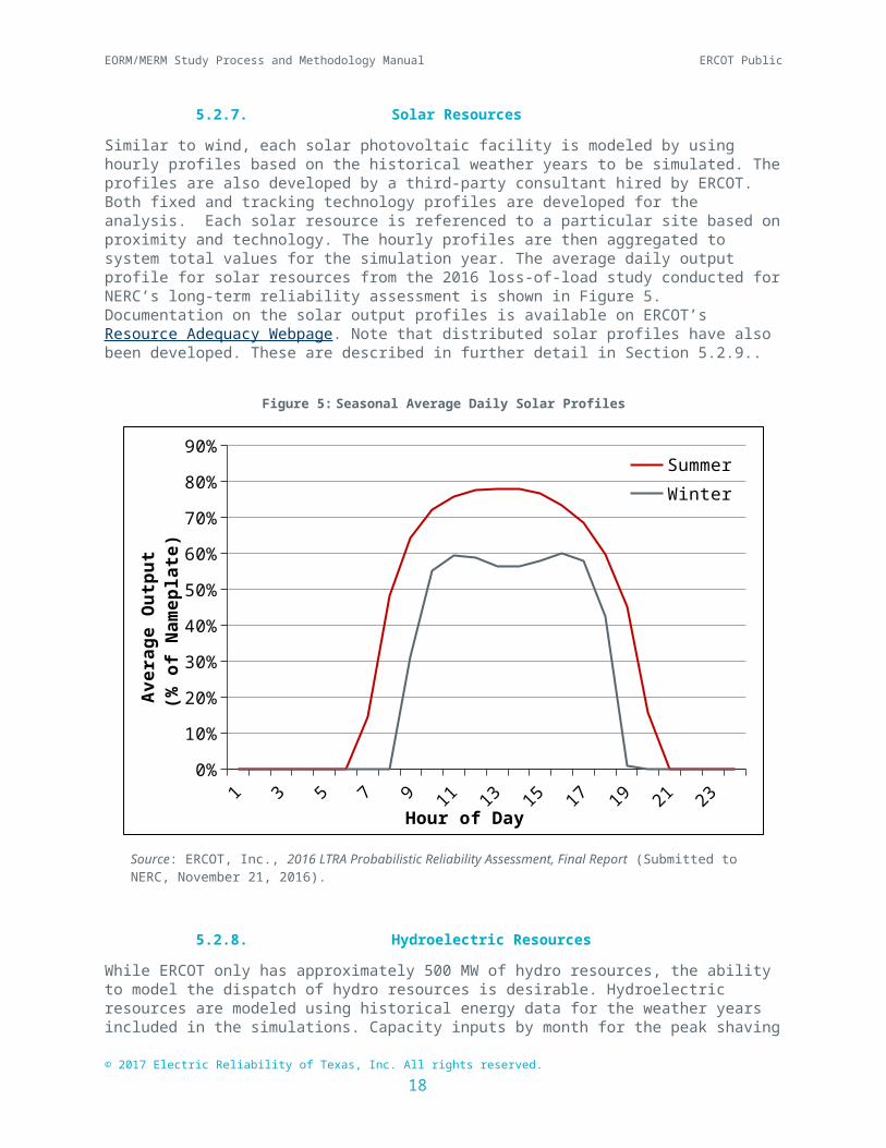
Similar to wind, each solar photovoltaic facility is modeled by using hourly profiles based on the historical weather years to be simulated. The profiles are also developed by a third-party consultant hired by ERCOT. Both fixed and tracking technology profiles are developed for the analysis. Each solar resource is referenced to a particular site based on proximity and technology. The hourly profiles are then aggregated to system total values for the simulation year. The average daily output profile for solar resources from the 2016 loss-of-load study conducted for NERC’s long-term reliability assessment is shown in Figure 5. Documentation on the solar output profiles is available on ERCOT’s Resource Adequacy Webpage. Note that distributed solar profiles have also been developed. These are described in further detail in Section 5.2.9.
10 ERCOT is investigating the efficacy and cost of having a consultant develop a set of stochastic wind profiles for each historical weather year that reflect realistic wind output variability based on the hourly weather conditions. If ERCOT decides to develop such stochastic wind profiles, this manual will be updated as dictated by the implementation timeline for the wind profile project.
© 2017 Electric Reliability of Texas, Inc. All rights reserved. 14
1 2 3 4 5 6 7 8 9 10 11 12 13 14 15 16 17 18 19 20 21 22 23 240%
10%
20%
30%
40%
50%
60%
Coastal Summer
Coastal Winter
Non Coastal Summer
Non Coastal Winter
Hour of Day
Aver
age
Out
put
(% o
f Nam
epla
te)

EORM/MERM Study Process and Methodology Manual ERCOT Public
Figure 5: Seasonal Average Daily Solar Profiles
1 2 3 4 5 6 7 8 9 1011121314151617181920212223240%
10%
20%
30%
40%
50%
60%
70%
80%
90%SummerWinter
Hour of Day
Ave
rage
Out
put
(% o
f Nam
epla
te)
Source: ERCOT, Inc., 2016 LTRA Probabilistic Reliability Assessment, Final Report (Submitted to NERC, November 21, 2016).
5.2.8. Hydroelectric Resources
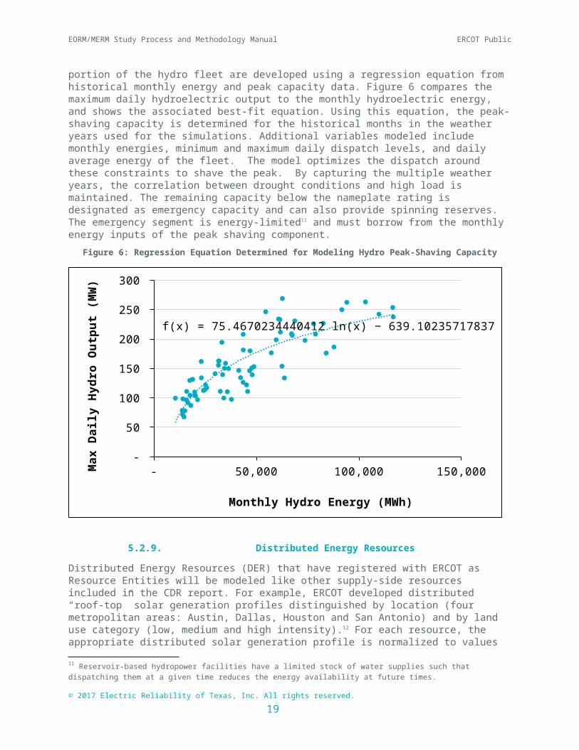
While ERCOT only has approximately 500 MW of hydro resources, the ability to model the dispatch of hydro resources is desirable. Hydroelectric resources are modeled using historical energy data for the weather years included in the simulations. Capacity inputs by month for the peak shaving portion of the hydro fleet are developed using a regression equation from historical monthly energy and peak capacity data. Figure 6 compares the maximum daily hydroelectric output to the monthly hydroelectric energy, and shows the associated best-fit equation. Using this equation, the peak-shaving capacity is determined for the historical months in the weather years used for the simulations. Additional variables modeled include monthly energies, minimum and maximum daily dispatch levels, and daily average energy of the fleet. The model optimizes the dispatch around these constraints to shave the peak. By capturing the multiple weather years, the correlation between drought conditions and high load is maintained. The remaining capacity below the nameplate rating is designated as emergency capacity and can also provide spinning reserves. The emergency segment is energy-limited11 and must borrow from the monthly energy inputs of the peak shaving component.
11 Reservoir-based hydropower facilities have a limited stock of water supplies such that dispatching them at a given time reduces the energy availability at future times.
© 2017 Electric Reliability of Texas, Inc. All rights reserved. 15

EORM/MERM Study Process and Methodology Manual ERCOT Public
Figure 6: Regression Equation Determined for Modeling Hydro Peak-Shaving Capacity
- 20,000 40,000 60,000 80,000 100,000 120,000 140,000 -
50
100
150
200
250
300
f(x) = 75.4670234440411 ln(x) − 639.10235717837
Monthly Hydro Energy (MWh)
Max
Dai
ly H
ydro
Out
put (
MW
)
5.2.9. Distributed Energy Resources
Distributed Energy Resources (DER) that have registered with ERCOT as Resource Entities will be modeled like other supply-side resources included in the CDR report. For example, ERCOT developed distributed “roof-top” solar generation profiles distinguished by location (four metropolitan areas: Austin, Dallas, Houston and San Antonio) and by land use category (low, medium and high intensity).12 For each resource, the appropriate distributed solar generation profile is normalized to values from zero to one and then multiplied by the capacity of the solar facility to yield properly scaled profiles.
Another DER category reflected in the RM Study are so-called “non-registered” resources. These resourcesone MW or less in size that never inject power into the gridare reflected as load reductions in the Long-Term Load and Energy Forecast rather than supply-side resources.
5.2.10. Energy Storage Technologies
Battery energy storage and pump storage technologies are economically dispatched in SERVM and can serve both energy and ancillary services. Inputs into SERVM include capacity, pumping/charging efficiency, pond reservoir/storage duration, and ancillary service eligibility. SERVM will optimize the use of the energy storage product to generate during high priced hours and pump/charge during off peak hours.
12 For details on the distributed solar profiles, see the report entitled, Solar Site Screen and Hourly generation Profiles, at http://www.ercot.com/content/wcm/lists/114800/ERCOT_Solar_SiteScreenHrlyProfiles_Jan2017.pdf
© 2017 Electric Reliability of Texas, Inc. All rights reserved. 16

EORM/MERM Study Process and Methodology Manual ERCOT Public
5.3. Fuel Prices
Fuel prices for gas, coal, and oil-fired plants are modeled for each month of the study year for each market. Based on feedback from the stakeholder EORM/MERM Workshop13, New York Mercantile Exchange (NYMEX) futures prices for coal, gas, and oil will be used as the main data source. ERCOT may assess and incorporate other price forecast information in light of futures market illiquidity for deliveries during the simulation year.
In addition to futures prices, ERCOT will develop locational delivered fuel price basis adders.14 Each basis adder will be determined by comparing historical delivered fuel prices for plants in the ERCOT Region to market price points (Houston Ship Channel, Waha, Carthage and TETCO STX). The fuel price for each generation unit in the model will be the futures price plus the appropriate locational basis adder. Fuel price sensitivity simulations will be developed to determine the impact of higher and lower prices on the MERM value.
Finally, ERCOT will attempt to maintain approximate consistency with the price forecasts used for Long-Term System Assessment (LTSA) resource expansion modeling.15 Changes in the price forecast methodologies, and the rationale for such changes, will be highlighted in the Study Plan. Significant deviations with respect to the LTRA price forecasts will be discussed in the RM Study report.
6. Demand-Side Resource Modeling
This section describes the modeling methodologies for Demand Response (DR) programs and energy efficiency. Demand Response resources consist of two broad categories: dispatchable and non-dispatchable. Dispatchable DR constitutes programs for which demand reduction events are initiated by ERCOT, whereas non-dispatchable DR constitutes demand reduction events initiated by the customer in response to price signals, or by the customer’s retail electric provider (REP) as part of standard contract terms. Energy efficiency, the third category of demand-side resources, is covered last in this section.
6.1. Dispatchable Resources
The two ERCOT dispatchable DR programs include Emergency Response Service (ERS) and Load Resources providing Ancillary Services (AS).16 Dispatchable DR resources are modeled with maximum available capacities (as reflected in the most current mid-year CDR report) and program call limits reflecting seasonal, daily, and hourly availability characteristics. Table 5 summarizes these call limit characteristics.
13 The Workshop was held on April 14, 2017. Workshop documentation is available at: http://www.ercot.com/calendar/2017/4/14/11745914 The basis adder reflects the contractual cost of delivering the fuel to the local gas utility.15 The LTSA report is filed with the PUCT and Texas Legislature during each even-numbered year. Modeling input assumptions are developed during the odd-numbered years. For example, assumptions for the 2018 LTRA are developed in 2017.16 The Ancillary Services that DR can provide include Responsive Reserves, Regulation-Up, Regulation-Down, and Non-Spin Reserves. For Responsive Reserves, LRs that are non-controllable (where the load reduction action is triggered by an Under Frequency Relay) are capped at a maximum of 50% of ERCOT’s total Responsive Reserve requirement.
© 2017 Electric Reliability of Texas, Inc. All rights reserved. 17

EORM/MERM Study Process and Methodology Manual ERCOT Public
Table 5: Call Limits for Demand Response Programs
Program Type Call Limits
Load Resources Serving as Responsive Reserves Unlimited
Emergency Response Service, 10-Min
8 hours per season and per hourly intervals; Seasons: Winter, Spring, Summer, Fall;
Hourly intervals: week day hours 1-8 and 21-24 and weekends, week day hours 9-13, week day hours 14-16, week day hours 17-20Emergency Response Service,
30-Min
As an example of how DR programs are specified for production cost modeling, Table 6 provides a list of the DR resource variables in the SERVM model.
Table 6: SERVM Demand-Response Variables
Variable Descriptionagc_capable Resource can provide Regulation service (Yes or No)
capmax Maximum capacity that can be input by month or can vary with hourly temperature (MW)
Condpw Demand Response Constraint - (Days Per Week)
Conhpd Demand Response Constraint - (Hours Per Day)
Conhpm Demand Response Constraint - (Hours Per Month)
Conhpy Demand Response Constraint - (Hours Per Year)
cstvar Variable O&M ($/MWh)
CurtailPrice The price at which a demand response resource is called in the supply stack ($/MWh)
hpy_emonth
Peaking units with hours per year (thermalhpy) operating constraints can narrow down the period of available operation. This variable defines the end month for the constraint. Also applies to demand response units. (Month)
hpy_smonth
Peaking units with hours per year (thermalhpy) operating constraints can narrow down the period of available operation. This variable defines the start month for the constraint. Also applies to demand response units. (Month)
Load_responsive_demand_idIndicates the load responsive demand curve for a specific demand response resource. This is used for modeling price responsive resources that provide more or less output during higher load periods.
Load_responsive_demand_randomThe default setting for the random draws using the load_responsive_demand curve is performed on a daily basis. To perform these draws hourly, the load_responsive_demand_random should be Y.
Max_dispatch_per_day
Represents the maximum number of times the Demand Response resource can be called in a single day. Differs from hours because the resource can be called for consecutive hours, which is counted as only one dispatch.
Max_dispatch_per_month
Represents the maximum number of times the Demand Response resource can be called in a single month. Differs from hours because the resource can be called for consecutive hours which is counted as only one dispatch. (dispatches)
Max_dispatch_per_yearRepresents the maximum number of times the Demand Response resource can be called in a year. Differs from hours because the resource can be called for consecutive hours which is counted as only one dispatch.
© 2017 Electric Reliability of Texas, Inc. All rights reserved. 18
EORM/MERM Study Process and Methodology Manual ERCOT Public
Variable Description
Min_dispatch_per_year
Represents the minimum number of times the Demand Response resource can be called in a single year. Different from hours because the resource can be called for consecutive hours which is counted as only one dispatch. Market prices from the initialization iterations are used to develop dispatches to meet this requirement.
Mindwn Represents the minimum number of consecutive hours that a Demand Response resource must be called
Period_availability For Demand Response resources, a period_availability can be assigned which points to specific portions of the week when the unit is available.
Price_responsive_demand_idIndicates the price-responsive demand curve for a specific Demand Response resource. This is used for modeling price-responsive resources that provide more or less output at higher pricing.
Price_responsive_demand_random
The default setting for the random draws using the price_responsive_demand curve, which is performed on a daily basis. To perform these draws hourly, the price_responsive_demand_random should be Y.
quickstartunit The resource can provide non-spin reserves (Yes or No)
Response_magnitude Enter multiple values as a uniform distribution to represent the percentage of capmax that is expected from the Demand Response resource. (%)
Rspprb Response probability for a Demand Response contract. Reflects the likelihood that load management program responds when called. (%)
The DR resources are dispatched for energy based on an emergency trigger, and in ascending order of their marginal costs. The marginal costs will be determined by analyzing ERCOT’s historical market data at the time that DR events occurred, dating back to 2011. Refer to Table 8 for the characteristics of all emergency procedures modeled. Any changes in ORDC implementation will be incorporated into the DR resource modeling assumptions.
6.2. Non-dispatchable Resources
Non-dispatchable DR resources that will be reflected in the RM Study include: (1) Standard Offer Programs managed by Transmission and/or Distribution Service Providers (TDSPs), and (2) price-responsive demand (PRD) reductions. Price-responsive demand refers to customers that voluntarily reduce or shift their energy use in response to dynamic pricing or tariff options offered by their electricity supplier. This resource category also includes Four Coincident Peak (4CP) price response behavior.17
As with ERS and “Load Resources Serving as Responsive Reserves”, TDSP Standard Offer Programs will be modeled with the mid-year CDR report’s maximum available system capacity18, program call limits, and a marginal cost. The call limits are currently specified as 16 hours per year during hours 14-20, for the summer months only (June-September). The marginal costs will be
17 Many industrial customers are subject to transmission charges based upon a Four Coincident Peak demand. The 4CP demand is determined by averaging the consumer’s actual demand for the 15-minute settlement interval with the highest ERCOT demand during each of the four summer months (June-September). This measured 4CP demand serves as the basis of the customer’s transmission tariff charges for the following year. By correctly predicting the ERCOT system peaks during the summer and curtailing load during those intervals, a consumer can reduce its transmission charges.18 For the CDR report, ERCOT uses the utility annual Verified Load Management Savings amounts reported by the PUCT.
© 2017 Electric Reliability of Texas, Inc. All rights reserved. 19
EORM/MERM Study Process and Methodology Manual ERCOT Public
determined by analyzing ERCOT’s historical market data at the time that DR events occurred, dating back to 2011.
ERCOT’s load forecast model is currently based on five years of historical data, and thereby captures the historical load reduction trends due to PRD actions. To introduce dynamic supply behavior of PRD in response to price signals, ERCOT will develop a probabilistic resource supply curves similar in concept to the PUN supply curves described in Section 5.2.4. The probabilistic PRD supply curves will be developed as follows:
Estimate the quantity of PRD in ERCOT. Compare the historical forecasted versus actual load shapes over the top load hours across several historical years, before considering price as an explanatory variable in realized load.
Estimate the price levels at which PRD has responded. Conduct an analysis to estimate the level of load reductions as a function of market price, as well as characterizing the uncertainty of PRD as a function of price.
Scale up the ERCOT load duration curve to account for PRD. Increase the ERCOT load duration curve in the peak hours above the forecast to account for the expected level of PRD reductions embedded within the load forecast.
Account for PRD as a probabilistic supply-side resource. Create a probabilistic representation of PRD that captures uncertainty in the quantity of PRD realized. For example, for the 2014 RM Study, PRD supply curves were developed with 13 market price levels ranging from $250/MWh to $9,000/MWh. Application of uniform draw probabilities of 5% thus resulted in 20 PRD quantities that the model can select for each market price level.
Historical 4CP price response behavior is also embedded in ERCOT’s load forecast. At the EORM/MERM Workshop, ERCOT discussed the possibility of building separate 4CP demand response supply curves. After careful consideration, ERCOT decided to develop supply curves for PRD exclusive of 4CP impacts due to the complexity of isolating and representing the 4CP response in a dynamic fashion.
6.3. Energy Efficiency
ERCOT’s load forecast model also captures historical load reduction trends due to energy efficiency measures. For the RM Study, energy efficiency measures will not be modeled explicitly. ERCOT assumes that future deviations from the historical energy efficiency trend embedded in the ERCOT load forecast can be adequately represented through the non-weather load uncertainty modeling approach described in Section 4.3.
7. Transmission System Modeling
This section describes the “hub-and-spoke” transmission system modeling framework to be used for the RM Study.
7.1. Transmission Topology
As noted in Section 3, multi-area modeling capability is needed to represent the impact of power imports and exports to neighboring power grids. To appropriately represent power flows to and from
© 2017 Electric Reliability of Texas, Inc. All rights reserved. 20

EORM/MERM Study Process and Methodology Manual ERCOT Public
SPP and Mexico, a three-region topology will be configured in the model. In addition to an ERCOT region, two external regions will be modeled with hourly loads and resources. Power sharing among the regions is based on economics and physical import/export limits. Internal transmission constraints for the ERCOT region will not be modeled. Representation of such internal constraints is not necessary unless regional reserve margin analysis becomes part of the study scope. More importantly, the topological granularity needed to adequately represent such transmission constraints in the model is currently prohibitive in terms of data preparation and the resulting model run-time requirements for executing thousands of annual scenarios.
7.1.1. Transmission Intertie Availability
The inter-regional transmission capacity constraints will represent the non-synchronous DC tie import/export capability between ERCOT and its neighbors. A distribution of capacity values will be used to reflect the probability of line outages. The actual imports into the model will be analyzed to ensure the simulations calibrate well with historical data.
7.1.2. Import/Export Mechanics during Scarcity Conditions
The model will schedule ERCOT imports and exports depending on the relative cost of production compared to neighboring systems. Import availability during scarcity conditions will therefore be modeled based on energy market prices. The 2014 RM Study modeled imports as available at prices of $20 - $250/MWh, and up to $1,000/MWh during capacity shortages.
8. Representation of ERCOT Markets
ERCOT, with consultant support, will develop inputs and a model configuration that best represents the ERCOT market at the time the study is conducted. The following sections describe the various market constructs and associated parameters needed to conduct the RM Study.
8.1. Energy and Ancillary Service Markets
To calculate the EORM and the MERM, the study will model the energy and ancillary service markets consistent with current market rules, operating procedures, and historical operation patterns.
The study will assume that all suppliers offer into the market at prices reflecting their marginal costs, including unit commitment costs. During non-scarcity hours, energy and ancillary prices and system costs will be based on the variable cost of the marginal supplier. During scarcity conditions, prices will reflect market-based and administrative emergency actions.
8.2. Scarcity Conditions
The study will account for all market-based and administrative emergency actions implemented during scarcity conditions, consistent with market rules and historical data. Accurately estimating the economically optimal reserve margin requires careful representation of the nature, trigger order, and marginal costs realized during each type of scarcity event.
© 2017 Electric Reliability of Texas, Inc. All rights reserved. 21

EORM/MERM Study Process and Methodology Manual ERCOT Public
8.2.1. Administrative Market Parameters
Prices during emergency events are primarily driven by two administrative constructs: the Operating Reserve Demand Curve (ORDC) and the Power Balance Penalty Curve (PBPC).19 These constructs rely on administratively-set parameters, including the Value of Lost Load (VOLL), the High System-Wide Offer Cap (HCAP), the Low System-Wide Offer Cap (LCAP), and the Peaker Net Margin (PNM) Threshold.20 Table 7 identifies the scarcity pricing parameters as of the 2014 study; the parameters will be updated with each MERM/EORM study as needed.
Table 7: ERCOT Scarcity Pricing Parameters Assumed for 2016 (2014 RM Study)
Parameter Value Notes
Value of Lost Load $9,000/MWh Administrative and actual
High System-Wide Offer Cap $9,000/MWh Always applies to ORDC
Low System-Wide Offer Cap $2,000/MWh Applies only to PBPC
Peaker Net Margin Threshold $291,000/MW-yr 3 x CT CONE
Consistent with market rules, the study will calculate Peaker Net Margin (PNM) over the calendar year and reduce the System-Wide Offer Cap (SWOC) to the Low System-Wide Offer Cap (LCAP) after the PNM threshold is exceeded. The change in SWOC from the HCAP to the LCAP affects the PBPC but not the ORDC calculations. ORDC remains a function of VOLL. See Section 8.2.5 for more detail.
8.2.2. Emergency Procedures and Marginal Costs
The RM Study will account for all emergency procedures and market responses to scarcity conditions. Responses can be of two types: market-based responses to high prices, and administrative actions triggered by emergency conditions. The RM Study will account for the price at which each response occurs and the marginal system cost of the response. This accounting will be developed based on a review of historical emergency event data and ERCOT’s emergency procedure manuals.21
Table 8 summarizes the emergency procedures modeled in the 2014 RM Study, the trigger order of each response as market prices rise, and the marginal cost of each response type. ERCOT and the RM Study consultant(s) will update the procedures, trigger order, and marginal cost of each resource type as needed.
19 See ERCOT Nodal Protocols Section 6.5.7.3. Available at http://www.ercot.com/mktrules/nprotocols/current20 See ERCOT Nodal Protocols Section 4.4. Available at http://www.ercot.com/mktrules/nprotocols/current21 See ERCOT (2013). Back Cast of Interim Solution B+ to Improve Real-Time Scarcity Pricing, White Paper, March 21, 2013 and ERCOT Market Guides: Nodal Operating Guides. Available at http://www.ercot.com/mktrules/guides/noperating/
© 2017 Electric Reliability of Texas, Inc. All rights reserved. 22

EORM/MERM Study Process and Methodology Manual ERCOT Public
Table 8: Emergency Procedures and Marginal Costs (2014 RM Study)
Emergency Level
MarginalResource Trigger Price Marginal System Cost
n/a Generation Price Approximately $20-$250 Same
n/a Imports PriceApproximately $20-$250Up to $1,000 during load
shedSame
n/a Non-Spin Shortage
PriceMarginal Energy +
Non-Spin ORDC w/ X = 2,000
Marginal Energy +Non-Spin ORDC w/ X = 1,150
n/aEmergency Generation
Price $500 Same
n/aPrice-
Responsive Demand
Price $250-$9000 Same
n/a Spin Shortage PriceMarginal Energy + Non-Spin
+ Spin ORDC w/ X = 2,000
Marginal Energy + Non-Spin+ Spin ORDC w/ X = 1,150
n/aRegulation Shortage
Price Power BalancePenalty Curve
Same(Unless Capped by LCAP)
EEA 130-Minute
ERSSpin ORDC x-axis
= 2,300 MW$3,239 at Summer Peak
(from ORDC)$1,405
EEA 1TDSP Load Curtailments
Spin ORDC x-axis= 1,750 MW
$9,000(from ORDC)
$2,450
EEA 2 Load Resourcesin RRS
Spin ORDC x-axis= 1,700 MW
$9,000(from ORDC)
$2,569
EEA 210-Minute
ERSSpin ORDC x-axis
= 1,300 MW$9,000
(from ORDC)$3,681
EEA 3 Load Shed Spin ORDC x-axis= 1,150 MW
VOLL = $9,000 Same
Sources and Notes: Developed based on review of historical emergency event data, input from ERCOT staff, and ERCOT’s emergency procedure manuals; see ERCOT Nodal Protocols, Section 6.5.9.4 and ERCOT Market Guides: Nodal Operating Guides
8.2.3. Emergency Generation
ERCOT will estimate the quantity and cost of emergency generation from suppliers who output power above their normal capacity ratings at the request of ERCOT. This information will be used to create a proxy generator that will be dispatched as needed. For example, the 2014 RM Study included an emergency generator reflecting the aggregate amount of emergency capacity that could be available above the sustained summer ratings used in the CDR, 360 MW. The 2014 RM Study
© 2017 Electric Reliability of Texas, Inc. All rights reserved. 23
EORM/MERM Study Process and Methodology Manual ERCOT Public
modeled emergency generation probabilistically assuming a 50% chance of realizing either 230 MW or 360 MW, at an assumed marginal cost of $500/MWh.
8.2.4. Operating Reserve Demand Curve
The ORDC reflects the willingness to pay for spinning and non-spinning reserves in the real-time market. Consistent with ERCOT’s ORDC implementation, the RM Study will model all distinct ORDC curves, which vary by season, time of day, and reserve type (separate ORDCs for spinning reserves and for spinning + non-spinning reserves).22 The study will calculate: (a) non-spin prices using the non-spin ORDC; (b) spin prices as the sum of the non-spin and spin ORDC; and (c) energy prices as the sum of the marginal energy production cost plus the non-spin and spin ORDC prices.
The spin ORDC will include all resources providing regulation-up or RRS, suppliers that are online but dispatched below their maximum capacity, hydro-synchronous resources, non-controllable load resources, and 10-minute quick start units. The spin + non-spin ORDC will include all resources contributing to the spin ORDC as well as any resources providing NSRS and all 30-minute quick start units.
The study will construct the price-setting ORDC consistent with the ORDC design assumption that ERCOT would shed load if spin + non-spin reserves were to fall below 2,000 MW. The study will separately estimate the level of reserves at which ERCOT operators will actually shed load by reviewing ERCOT operations during recent emergency events, and use this level of spin + non spin reserves to construct a second ORDC that shifts the price-setting ORDC to the estimated load shed threshold. Figure 7 illustrates an example price-setting ORDC and marginal cost ORDCs from the 2014 RM Study.
The 2014 RM Study found ERCOT would shed load if spinning + non-spinning reserves were to fall below 1,150 MW. The discrepancy between the 1,150 MW load shed threshold and the ORDC-assumed 2,000 MW threshold resulted in prices above marginal costs during moderate scarcity pricing events, resulting in the MERM higher than the EORM.
22 See ERCOT and Hogan (2013). Back Cast of Interim Solution B+ to Improve Real-Time Scarcity Pricing, White Paper, March 21, 2013.
© 2017 Electric Reliability of Texas, Inc. All rights reserved. 24

EORM/MERM Study Process and Methodology Manual ERCOT Public
Figure 7: Operating Reserve Demand Curves (2014 Study)
Sources and Notes: Red: Price-setting ORDC. Blue: Marginal cost ORDC. Example curves for summer hours 15 – 18. ORDC curves developed consistent with, ERCOT and Hogan (2013). Back Cast of Interim Solution B+ to Improve Real-Time Scarcity Pricing, White Paper, March 21, 2013.
8.2.5. Power Balance Penalty Curve
The PBPC is an ERCOT market mechanism that introduces administrative scarcity pricing during periods of supply shortages. Consistent with how ERCOT incorporates the PBPC into the security constrained economic dispatch (SCED) software, the study will model the PBPC as phantom supply that may influence the realized price, and that will cause a reduction in available regulating reserves whenever called. The price/quantity pairs for each phantom generator will be consistent with current ERCOT market rules.23
At the highest price, the PBPC will reach the system-wide offer cap (SWOC), which is set at the HCAP at the beginning of each calendar year but which will drop to the LCAP + $1/MWh once the PNM threshold is exceeded. For purposes of estimating the EORM, the study will assume that the prices in the PBPC are reflective of the marginal cost incurred by going short of each quantity of regulating reserves. Figure 8 illustrates the PBPC in 2013 and the 2016 PBPC assumed in the 2014 study.
23 See ERCOT Business Practice: Setting the Shadow Price Caps and Power Balance Penalties in Security Constrained Economic Dispatch, Public, Version_8.0, effective July 17, 2013. Available at http://www.ercot.com/content/mktinfo/rtm/kd/Methodology%20for%20Setting%20Maximum%20Shadow%20Prices%20for%20Network%20an.zip
© 2017 Electric Reliability of Texas, Inc. All rights reserved. 25

EORM/MERM Study Process and Methodology Manual ERCOT Public
Figure 8: Power Balance Penalty Curve (2014 Study)
Sources and Notes: Year 2016 PBPC updated in approximate proportion to the scheduled increases in system price cap, as rounded up or down consistent with ERCOT staff guidance. 2013 PBPC numbers from ERCOT (2013), p. 23. See ERCOT Business Practice: Setting the Shadow Price Caps and Power Balance Penalties in Security Constrained Economic Dispatch, Public, Version_8.0, effective July 17, 2013. Available at http://www.ercot.com/content/mktinfo/rtm/kd/Methodology%20for%20Setting%20Maximum%20Shadow%20Prices%20for%20Network%20an.zip
8.3. Generator Cost of New Entry (CONE)
The Gross Cost of New Entry (CONE) parameter reflects the annualized fixed costs of building and operating a new resource. The study will use a CONE estimate for the marginal resource technology that accounts for all capital costs, fixed costs, and the after-tax weighted-average cost of capital (ATWACC).
ERCOT does not regularly conduct bottom-up engineering studies of CONE, and such an analysis is outside the scope of the RM Study. As such, the study may rely on public CONE studies from other RTOs, adjusted for locational cost differences due to factors including the cost of capital, labor productivity and rates, taxes, delivery charges, and weather-related construction interruptions. If studies from other RTOs cannot be reliably used, the study may instead use capital cost estimates from ERCOT studies such as the Long-Term System Assessment. The 2014 RM study relied on modified CONE estimates from PJM Interconnection LLC (PJM), with adjustments applied as relevant to ERCOT (see Table 9).24 As CONE is uncertain and a major driver of both the EORM and MERM, ERCOT will conduct sensitivity simulations of this parameter as part of its EORM/MERM uncertainty analysis. (See Section 9.5 for more details.) For example, the 2014 RM Study tested a CONE range of -10% to +25%.24 See Newell, Samuel, et al. (2012), ERCOT Investment Incentives and Resource Adequacy, prepared for ERCOT, June 1, 2012. And Spees, Kathleen, Samuel A. Newell, Robert Carlton, Bin Zhou, and Johannes P. Pfeifenberger. (2011) Cost of New Entry Estimates for Combustion Turbine and Combined-Cycle Plants in PJM. August 24, 2011.
© 2017 Electric Reliability of Texas, Inc. All rights reserved. 26
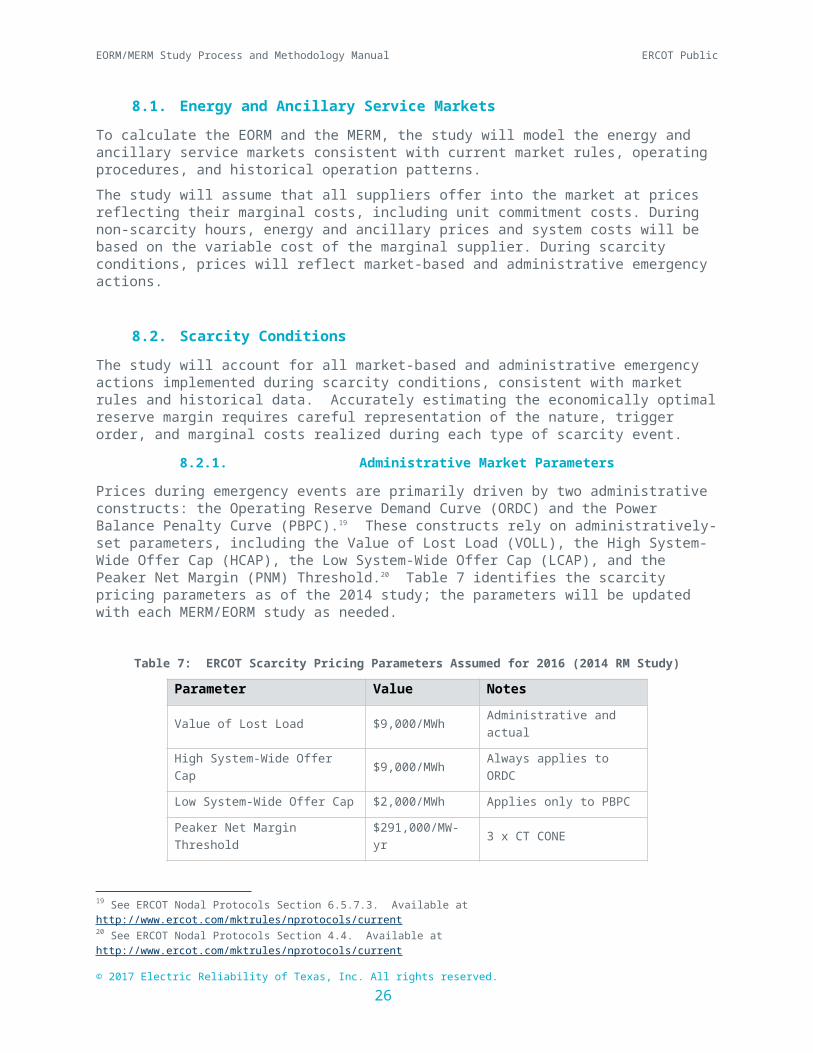
EORM/MERM Study Process and Methodology Manual ERCOT Public
Table 9: Gross Cost of New Entry (2014 Study)
ATWACC (%/yr)
Gross CONE: Simple Cycle
($/MW-yr)
Gross CONE: Combined Cycle
($/MW-yr)From 2012 CONE Study (2015 Online Date)
Low: Merchant ATWACC 7.6% $90,100 $112,400
Mid: ERCOT Planning Assumption 9.6% $105,000 $131,000
High: Developer-Reported 11.0% $131,000 $145,000
Updated Estimate (2016 Online Date)
Low: Base minus 10% n/a $87,300 $109,900
Base: Merchant ATWACC 8.0% $97,000 $122,100
High: Base plus 25% n/a $121,300 $152,600
Sources and Notes: 2012 Study numbers and current numbers adapted from a CONE study for PJM, with adjustments applied as relevant for ERCOT, see Newell et al. (2012)25 and Spees et al. (2011).26 Updated estimate applies 4.3% and 5.2% escalation derived from Newell et al. (2013).27
8.4. Value of Lost Load (VOLL)
The study will use a Value of Lost Load consistent with the high System-Wide Offer Cap (HCAP) set by the PUCT.28 The 2014 RM Study assumed an HCAP of $9,000/MWh.
9. Study Results
9.1. Reserve Margin Accounting
The reserve margin is calculated according to ERCOT’s CDR method, using the following formula:
PlanningReserve Margin=Total Resources−FirmPeak LoadFirmPeak Load
x100
Firm load is defined as the peak load minus demand response resources and energy efficiency. Total Resources include the following:
Thermal resources based on seasonal net sustained capability per CDR Hydro peak seasonal capacity contribution per CDR
25 Newell, et al. ERCOT Investment Incentives and Resource Adequacy, prepared for ERCOT, June 1, 201226 Spees, Kathleen, Samuel A. Newell, Robert Carlton, Bin Zhou, and Johannes P. Pfeifenberger. (2011) Cost of New Entry Estimates for Combustion Turbine and Combined-Cycle Plants in PJM. August 24, 2011.27 Newell, Samuel A., J. Michael Hagerty, and Quincy X. Liao. (2013). 2013 Offer Review Trigger Prices Study. Prepared for the ISO New England. October 2013. Filed before the Federal Energy Regulatory Commission in Docket ER14-616.28 See PUCT (2012), Electric Substantive Rules, Chapter 25, §25.505 Subchapter S, Section (g)(6). http://www.puc.texas.gov/agency/rulesnlaws/subrules/electric/25.505/25.505.pdf
© 2017 Electric Reliability of Texas, Inc. All rights reserved. 27
EORM/MERM Study Process and Methodology Manual ERCOT Public
Switchable capacity less amount unavailable per CDR Available mothballed and RMR capacity per CDR Private use network resources at capacity contribution forecast per CDR DC tie capacity contribution per CDR Planned thermal resources per CDR Installed and planned wind/solar, based on applying the seasonal peak-average capacity
contribution methodology outlined in Nodal Protocol Section 3.2.6.2.2 to the wind and solar shapes used in the model. (This ensures that the EORM and MERM values are consistent with the wind and solar resources as modeled.)
9.2. Total System Cost and Energy Margin
The RM Study report will include the weighted average Total System Cost at each simulated reserve margin level. Figure 9 is an example of the chart to be included. The calculation will account for and itemize all components of total system costs, including:
Capital Costs of the Marginal Resource Production Costs External System Costs (production and scarcity costs in neighboring systems) Emergency Generation Costs 10-Minute and 30-Minute Emergency Response Service Costs Non-Controllable Load Resource Costs TDSP Load Management Costs Price Responsive Demand Costs Spinning and Non-Spinning Reserve Shortage Costs Regulation Shortage Costs Firm Load Shedding Costs
Figure 9: Sample Chart Showing Weighted Average Total System Cost by Reserve Margin
26,600
26,650 26,700 26,750
26,800 26,850 26,900
26,950 27,000 27,050
8% 9% 10% 11% 12% 13% 14% 15% 16% 17%
Tota
l Sys
tem
Cos
ts M
$
Reserve Margin
EORM
© 2017 Electric Reliability of Texas, Inc. All rights reserved. 28
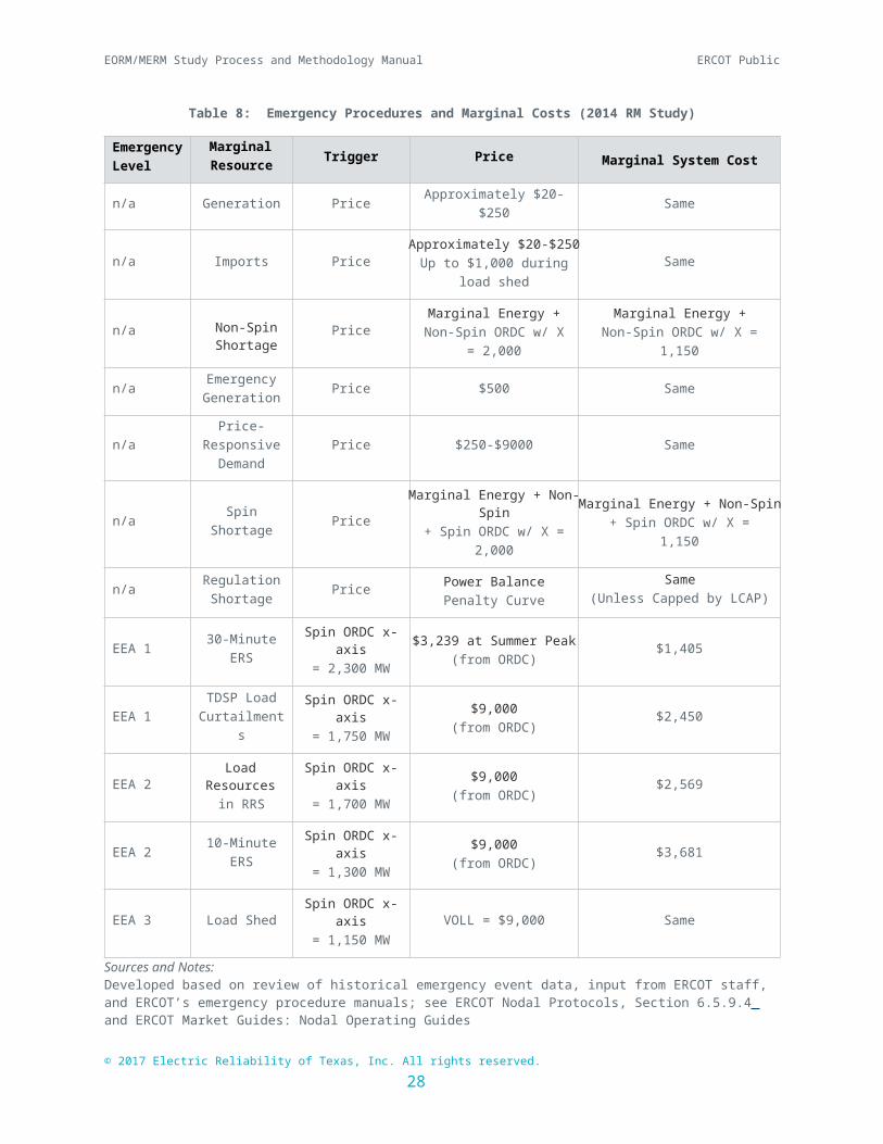
EORM/MERM Study Process and Methodology Manual ERCOT Public
The RM Study report will also include a chart that shows the energy margin29 (in dollars per kW-year) for the marginal resource at each simulated reserve margin level. See Figure 10 for a sample chart.
Figure 10: Sample Chart Showing Weighted Average Energy Margin by Reserve Margin
8.00%
9.00%
10.00%
11.00%
12.00%
13.00%
14.00%
15.00%
16.00%
17.00%
- 20 40 60 80
100 120 140 160 180
MERM
Reserve Margin
$/kW
-yr
9.3. Economically Optimal Reserve Margin
The Study will cite the EORM, the reserve margin at which total system costs are minimized. The Study will include the EORM for the Base Case and any Sensitivity Cases.
9.4. Market Equilibrium Reserve Margin
The study will report the MERM, the reserve margin that the current energy-only market design will likely support. The MERM may differ from the EORM if market prices during scarcity pricing events differ from marginal costs. The Study report will include the MERM for the Base Case and any Sensitivity Cases.
9.5. EORM and MERM Uncertainty Analysis
ERCOT will conduct in-scope sensitivity model runs and develop a tornado diagram to present the results. The tornado diagram is a horizontally displayed bar chart that provides a sorted highest-to-lowest comparison of the relative importance of different variables. To indicate the combined uncertainty range of all the sensitivity assumptions, ERCOT will run low and high sensitivity simulations where all the sensitivity values are set to generate low EORM/MERM values and high values, respectively. Figure 11 provides an illustrative tornado diagram using dummy data.
29 The formula for energy margin is as follows:Energy Margin = (annual energy revenues + annual ancillary service revenues - annual variable costs)/Capacity
where annual variable costs = fuel costs + variable O&M costs + startup costs + emission costs
© 2017 Electric Reliability of Texas, Inc. All rights reserved. 29
EORM/MERM Study Process and Methodology Manual ERCOT Public
Figure 11: Tornado Diagram for EORM Sensitivities
9.6. Physical System Reliability Standards
System reliability metrics based on meeting physical reliability standards, such as a 1-in-10 loss of load expectation standard (0.1 LOLE) will not be calculated as an in-scope activity of the RM Study.
9.7. Reporting a Reference Reserve Margin Level for NERC Reliability Assessments
9.7.1. Background on NERC’s Reference Margin Level
NERC prepares and publishes on an annual basis its Long-Term Reliability Assessment (LTRA). As part of the LTRA reporting effort, Regional Entities provide NERC with a capacity planning reserves “Reference Margin Level” along with capacity and demand data for the 10-year assessment period. NERC’s description and reporting instructions for the Reference Margin Level is provided in Figure 12. As mentioned in the Instructions, if a Regional Entity does not provide a Reference Margin Level for the LTRA data submission, then NERC will apply a default value of 15% for “predominately thermal” systems.
Figure 12: NERC Reference Margin Level Definition and Reporting Instructions
© 2017 Electric Reliability of Texas, Inc. All rights reserved. 30
6% 7% 8% 9% 10% 11% 12% 13% 14% 15% 16%
Combined Uncertainty
Sensitivity 1
Sensitivity 2
Sensitivity 3
Sensitivity 4
EORM
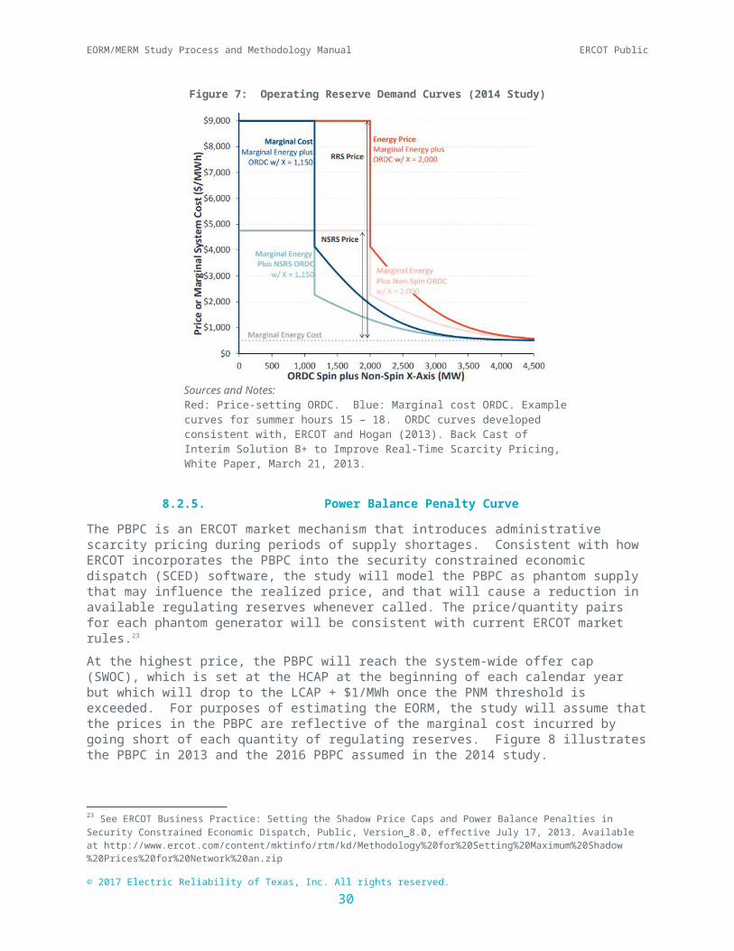
EORM/MERM Study Process and Methodology Manual ERCOT Public
Source: NERC 2017 Long-Term Reliability Assessment, Data Form Instructions, January 25, 2017.
The purpose of the Reference Margin Level is to serve as the threshold indicating whether there is a forecasted seasonal (summer and/or winter) shortfall of system peak-hour capacity reserves during the LTRA’s assessment period. The Reference Margin Level is also used for NERC’s summer and winter seasonal reliability assessment reports.
As the designated Assessment Area for the Texas Reliability Entity (TRE) Region, ERCOT reports to NERC the current Reference Margin Level for all assessment years. The Reference Margin Level is compared to what NERC refers to as the Anticipated Planning Reserve Margin. This Margin, expressed as a percentage, is defined as:
Anticipated PRM=( Anticipated ResourceCapacity+Net ExpectedCapacity Transfers – Net Internal DemandNet Internal Demand )x 100where,
Anticipated Resource Capacity = existing available capacity plus planned capacity that meets specified Assessment Area requirements such as having a signed Interconnection Agreement;Net Expected Capacity Transfers = expected imports less exports;Net Internal Demand = system demand reduced by the projected impacts of Controllable and Dispatchable Demand Response programs.
9.7.2. Use of the Reference Margin Level in NERC Reliability Assessments
If the Anticipated Planning Reserve Margin falls below the Reference Margin Level for any year, then NERC requires the Regional Entity/Assessment Area(s) to identify any potential reliability impacts of the forecasted capacity deficit, along with mitigation plans. This reporting requirement is outlined in NERC’s Rules of Procedure:
The assessment shall determine if the resource information submitted represents a reasonable and attainable plan for the Regional Entity and its members. For cases of inadequate capacity or reserve margin, the Regional Entity will be requested to analyze and explain any resource capacity inadequacies and its plans to mitigate the reliability impact of the potential inadequacies. The analysis may be expanded to include surrounding areas. If the expanded analysis indicates further inadequacies, then an interregional problem may exist and will be explored with the applicable Regions. The results of these analyses shall be described in the assessment report.30
9.7.3. Reporting a Reference Margin Level to NERC
Unless instructed to do otherwise by the PUCT, ERCOT will provide NERC with the MERM value cited in the RM Study. The RM Study report will be provided to NERC as supporting documentation for derivation of the Reference Margin Level cited in subsequent NERC reliability assessments.
30Section 805.1, Rules of Procedure of the North American Electric Reliability Corporation (Effective October 31, 2016), p. 68.
© 2017 Electric Reliability of Texas, Inc. All rights reserved. 31

EORM/MERM Study Process and Methodology Manual ERCOT Public
10. Appendices
© 2017 Electric Reliability of Texas, Inc. All rights reserved. 32
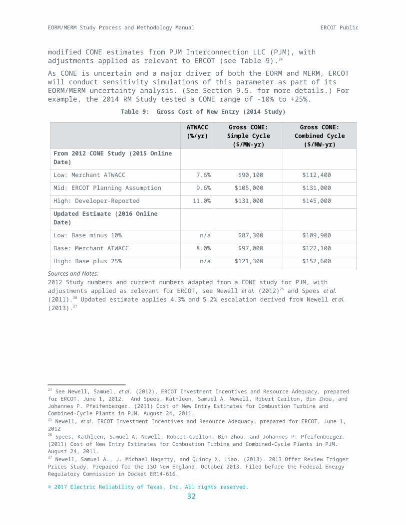
EORM/MERM Study Process and Methodology Manual ERCOT Public
10.1. Filed Letter to the PUCT on Conducting EORM/MERM Studies
© 2017 Electric Reliability of Texas, Inc. All rights reserved. 33

EORM/MERM Study Process and Methodology Manual ERCOT Public
© 2017 Electric Reliability of Texas, Inc. All rights reserved. 34

EORM/MERM Study Process and Methodology Manual ERCOT Public
10.2. Calculation of Probability Weights for Weather-year Load Forecasts
The development of historical weather-year probability weights is based on a six-step process:
1. Create an annual high ambient-temperature-based index intended to represent the weather-driven risk of experiencing Energy Emergency Alert (EEA) events for a given year. The higher the index value, the higher the risk of EEA events.
2. Apply a statistical method to the index values to determine mild and extreme outlier thresholds.
3. Develop a frequency histogram of the index values, and then calculate relative frequency percentages by dividing each frequency by the sum of the frequencies.
4. Demarcate the frequency histogram values (and associated relative frequency percentages) into low, moderate, high and extremely high risk ranges. The high and extremely high risk ranges are based on the mild and extreme outlier thresholds, respectively, from Step 2.
5. For each of the four risk ranges, determine a probability value for index values that fall within the range.
6. Assign a probability value to each index value; then normalize the probability values to the range [0, 1] such that the probability values sum to one.
The sections below provide more details on each step, and include data tables and sample calculations for an index range covering 1980 through 2016. This probability weighting approach was outlined at a SAWG meeting held on August 18, 2017.
10.2.1. Weather-risk Index
The chosen index is based on the number of consecutive days in a year that ambient “dry bulb” temperatures exceed 100 F in three major metropolitan areas within the ERCOT Region: Dallas-Fort Worth (DFW), Houston (IAH), and Austin (AUS). The “number of consecutive days” criterion recognizes that the probability of EEA events occurring is expected to increase during a sustained period of high loads. Table 10 is an extract of the temperature data set for 1980, showing each occurrence of consecutive-day temperatures for the three metro areas and the number of days for which occurrence. Austin had a total of 14 days where consecutive high temperatures occurred, Dallas-Fort Worth had 53 days, and Houston had 16 days.
Table 10: Consecutive Days of Temperatures exceeding 100 Degrees for 1980
© 2017 Electric Reliability of Texas, Inc. All rights reserved. 35
Weather Station
Dry Bulb
TempLast Date of
Consecutive Days Year CountAUS 100.6 6/29/1980 1980 3AUS 101.5 7/2/1980 1980 2AUS 100.6 7/13/1980 1980 2AUS 100.6 7/19/1980 1980 5AUS 100.6 7/24/1980 1980 2DFW 100.3 6/19/1980 1980 2DFW 100.6 7/23/1980 1980 31DFW 104.9 7/26/1980 1980 2DFW 101.5 8/3/1980 1980 7DFW 100.6 8/9/1980 1980 5DFW 101.5 8/25/1980 1980 6IAH 100.6 6/27/1980 1980 2IAH 100.6 7/2/1980 1980 3IAH 100.6 7/13/1980 1980 3IAH 100.6 7/19/1980 1980 5IAH 100.6 8/24/1980 1980 3

EORM/MERM Study Process and Methodology Manual ERCOT Public
To calculate the annual index value, the occurrence counts are first summed for each metro area. Each metro-area total is then multiplied by the areas’ load-share weight. The area load-share weights are calculated as the ratio of the Weather Zone31 summer peak load for the most recent year divided by the sum of Weather Zone peak loads. Finally, the weighted occurrence counts are summed to get the final index value. Table 11 shows the derivation of index values for two sample years, 1980 and 1987, indicating the index magnitude for relatively high and low weather-risk years, respectively. Figure 13 graphically shows all the index values for 1980 through 2016.
Table 11: Calculation of Weather Risk Index Values for 1980 and 1987
YearMetro Area
Consecutive High-Temp Occurrence
Count
Load Share
Weight
Weighted Occurrence
CountIndex Value
1980 AUS 14 0.21 2.9332.001980 DFW 53 0.44 23.51
1980 IAH 16 0.35 5.55
1987 AUS 0 0.21 0.001.331987 DFW 3 0.44 1.33
1987 IAH 0 0.35 0.00
Figure 13: Weather Risk Index Values, 1980-2016
10.2.2. Outlier Thresholds
Outlier detection for the index values uses a technique called the Quartile Fence Method. This method is basically the same one used for constructing box-and-whisker charts in Microsoft Excel and other charting applications. It is suitable for a data series that is not normally distributed and has a relatively small sample size (< 100 observations).
For this method, the 1st, 2nd, and 3rd quartiles are first calculated, as well as the Interquartile Range (IQR). The IQR is the 3rd quartile less the 1st quartile (IQR = Quartile3 – Quartile1). The Lower Fence, which is the threshold for mild outliers, has the simple formula, LF = Quartile3 + (1.5 x IQR).
31 Dallas-Fort Worth is assigned to the North Central zone, Houston is assigned to the Coastal zone, and Austin is assigned to the South Central zone.
© 2017 Electric Reliability of Texas, Inc. All rights reserved. 36
0.00
5.00
10.00
15.00
20.00
25.00
30.00
35.00
40.00
1980198119821983198419851986198719881989199019911992199319941995199619971998199920002001200220032004200520062007200820092010201120122013201420152016

EORM/MERM Study Process and Methodology Manual ERCOT Public
The Upper Fence, which is the threshold for extreme outliers, has the formula, UF = Quartile3 + (3 x IQR). Table 12 shows the Interquartile Fence parameters calculated from the index values. Index values that are between 19 and 29 are considered mild outliers, while index values greater than 29 are considered extreme outliers
Table 12: Quartile Fence Parameters
Interquartile Fence Parameters Values
Quartile1 1.77Quartile2 3.55Quartile3 8.67Interquartile Range 6.90Lower Fence 19.02Upper Fence 29.37
10.2.3. Frequency Histogram
Table 13 shows the histogram values (bins, frequencies, and relative frequency percentages) computed for the index range, whileError: Reference source not found is the resulting histogram. The relative frequency percentages are the bin frequencies divided by the total frequency count (n = 37).
Table 13: Weather-Risk Index Frequencies and Relative Frequency Percentages
Bin FrequencyRelative Frequency
Percentages0 6 0.16221 1 0.02702 5 0.13513 4 0.10814 4 0.10815 2 0.05416 3 0.08117 1 0.02708 1 0.02709 2 0.0541
10 1 0.027011 0 0.000012 1 0.027013 0 0.000014 1 0.027015 1 0.027016 0 0.000017 0 0.000018 0 0.000019 1 0.027020 0 0.000021 0 0.000022 0 0.0000
© 2017 Electric Reliability of Texas, Inc. All rights reserved. 37
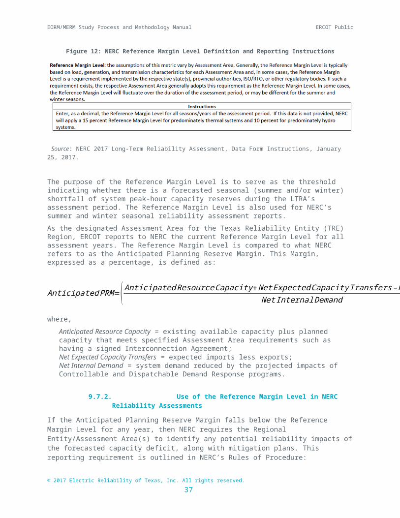
EORM/MERM Study Process and Methodology Manual ERCOT Public
Bin FrequencyRelative Frequency
Percentages23 0 0.000024 1 0.027025 0 0.000026 0 0.000027 0 0.000028 0 0.000029 0 0.000030 0 0.000031 0 0.000032 1 0.027033 0 0.000034 0 0.000035 0 0.000036 0 0.000037 1 0.0270
Figure 14: Weather-Risk Index Histogram
10.2.4. Identify Index Risk Ranges
The next step is to group ranges of index values into low, moderate, high and extremely high weather-risk categories. Index values of zero were assigned to the low risk category. The high and extremely high risk categories are defined by the Lower and Upper Fence threshold values (19 and 29, respectively). The remaining range of values, 1 through 18, are assigned to the moderate risk category. Table 14 shows the risk category assignments.
© 2017 Electric Reliability of Texas, Inc. All rights reserved. 38
0
1
2
3
4
5
6
7
0 1 2 3 4 5 6 7 8 9 10 11 12 13 14 15 16 17 18 19 20 21 22 23 24 25 26 27 28 29 30 31 32 33 34 35 36 37
Freq
uenc
y (N
= 3
7)
High Temperature Index Values
Histogram

EORM/MERM Study Process and Methodology Manual ERCOT Public
Table 14: Categorization of Index Values by Risk Level
Bin Frequency
Relative Frequency
Percentages Risk Category0 6 0.1622 Low1 1 0.0270
Moderate
2 5 0.13513 4 0.10814 4 0.10815 2 0.05416 3 0.08117 1 0.02708 1 0.02709 2 0.0541
10 1 0.027011 0 0.000012 1 0.027013 0 0.000014 1 0.027015 1 0.027016 0 0.000017 0 0.000018 0 0.000019 1 0.0270
High
20 0 0.000021 0 0.000022 0 0.000023 0 0.000024 1 0.027025 0 0.000026 0 0.000027 0 0.000028 0 0.000029 0 0.0000
Extremely High
30 0 0.000031 0 0.000032 1 0.027033 0 0.000034 0 0.000035 0 0.000036 0 0.000037 1 0.0270
10.2.5. Assigning Probabilities to the Risk Categories
All the index values falling into a risk category are assigned a probability of occurrence. For the low risk category, the probability is the relative frequency percentage for the zero value bin, 16.2%. Any year with an index value of zero (no consecutive days of temperatures greater than 100 F) has a 16.2% probability of occurring. The probability for the moderate risk category is the sum of the relative frequency percentages for index values assigned to the bins in this category, 73%.
© 2017 Electric Reliability of Texas, Inc. All rights reserved. 39

EORM/MERM Study Process and Methodology Manual ERCOT Public
The sparsity of mild and extreme outliers causes a complication in adding the relative frequency percentages for the high and extremely high risk categories. Since the number of mild and extreme outliers is the same (two each), the probability of occurrence is the same at 5.4% (2 x 0.027). A distinguishing metric must be applied to ensure that mild outliers have a higher probability of occurrence than extreme outliers. For this purpose, the approach is to calculate end-point distance ratios for index values in the high and extreme risk categories. The distance ratio indicates how close the average index value for a risk category is to the end-point of the index value range, in this case a value of 37. Since the distance ratio for the mild outliers will be larger than the one for extreme outliers, this metric can be used to weight the relative frequency percentages. Table 15 shows the calculation of the distance ratios and their conversion to probability weights that sum to one.
Table 15: Distance Ratio Calculations
Distance Ratio Parameters Values FormulaeAverage Index Value, High Risk Category 23.50
N/AAverage Index Value, Extreme High Risk Category 33.00 End-Point Index Value 37.00
Mild Outlier Distance Ratio 0.36 = (1 - (23.50 / 37.00)Extreme Outlier Distance Ratio 0.11 = (1 - (33.00 / 37.00)
Mild Outlier Probability Weight 0.77 = 0.36 / (0.36 + 0.11)Extreme Outlier Probability Weight 0.23 = 0.11 / (0.36 + 0.11)
To get the adjusted probabilities for the high and extremely high risk categories, the last step is to multiply the sum of the relative frequency percentages for all outliers (4 x 0.027 = 0.108) by the mild outlier probability weight (0.77) and extreme outlier probability weight (0.23), respectively. The adjusted probabilities are thus 8.3% and 2.5%. Note that the probabilities for the four risk categories sum to one.
10.2.6. Assigning Probabilities to the Weather Years
The last step is to assign one of the four risk category probabilities to each weather year. Table 16 shows how the probabilities are mapped. An index value falling into the specified ranges (middle column) are assigned the probabilities in the last column.
Table 16: Weather-Year Probability Assignment by Risk Category
Risk CategoryIndex Value
RangeProbability of
Occurrence (%)Low Risk 0.00 16.2
Moderate Risk 0.01 - 19.00 73.0High Risk 19.01 - 28.00 8.3
Extremely High Risk 28.01 - 37.00 2.5
Because these probabilities are applicable to a range of index values rather than to individual index values, the final calculation is to normalize the assigned weather-year probabilities so they sum to one. This is accomplished by dividing each weather-year probability by the sum of all the probabilities. Table 17 shows this derivation.
© 2017 Electric Reliability of Texas, Inc. All rights reserved. 40

EORM/MERM Study Process and Methodology Manual ERCOT Public
Table 17: Derivation of Weather-Year Probabilities
Weather Year
Risk Category Probability
Weather-Year Probability
1980 2.5% 0.1%1981 73.0% 3.4%1982 73.0% 3.4%1983 16.2% 0.8%1984 73.0% 3.4%1985 73.0% 3.4%1986 73.0% 3.4%1987 73.0% 3.4%1988 73.0% 3.4%1989 73.0% 3.4%1990 73.0% 3.4%1991 16.2% 0.8%1992 16.2% 0.8%1993 73.0% 3.4%1994 73.0% 3.4%1995 73.0% 3.4%1996 73.0% 3.4%1997 16.2% 0.8%1998 73.0% 3.4%1999 73.0% 3.4%2000 8.3% 0.4%2001 73.0% 3.4%2002 16.2% 0.8%2003 73.0% 3.4%2004 16.2% 0.8%2005 73.0% 3.4%2006 73.0% 3.4%2007 73.0% 3.4%2008 73.0% 3.4%2009 73.0% 3.4%2010 73.0% 3.4%2011 2.5% 0.1%2012 73.0% 3.4%2013 73.0% 3.4%2014 73.0% 3.4%2015 73.0% 3.4%2016 73.0% 3.4%
10.3. Incorporation of Stakeholder Comments in the Draft Manual
ERCOT issued a General Notice on November 3, 2017 specifying a 30-day public review period for the draft manual. Three parties provided comments or offered text edits by the review period deadline (December 4th). The substantive comments and ERCOT’s responses are summarized below.
© 2017 Electric Reliability of Texas, Inc. All rights reserved. 41

EORM/MERM Study Process and Methodology Manual ERCOT Public
10.3.1. Modeling of Price Responsive Demand (PRD)
One party provided edits to Section 6.2, “Non-dispatchable Resources.” The edits expanded the estimation of PRD load reductions as a function of price level to also include “the percentage of peak load” as an additional explanatory variable. The stated rationale for including peak load percentage is that it will help estimate the 4CP response contribution of PRD. ERCOT modified the paragraph in Section 6.2 to make it clear that the PRD supply curve will attempt to capture demand reduction exclusive of the 4CP response, which is already factored into the load forecast. This treatment is consistent with modeling strategy adopted for the 2014 RM Study.
10.3.2. NERC Reference Reserve Margin Level
Two parties commented on the wording of section 9.7.3, “Reporting a Reference Margin Level to NERC”. One party provided edits to the effect that ERCOT would accept NERC’s default Reference Reserve Margin Level (currently 15% for thermal-dominated systems) and provide EORM/MERM values to NERC for informational purposes only. The other party recommended that the MERM should be provided to NERC as the Reference Margin Level rather than the higher of the EORM and MERM values. ERCOT adopted the latter suggestion, changing the relevant text to the following: “Unless instructed to do otherwise by the PUCT, ERCOT will provide NERC with the MERM value cited in the RM Study.”
10.3.3. Resource Costs
One party recommended that ERCOT use Verifiable Costs as appropriate for resource modeling. ERCOT believes that this proposal should be discussed at relevant Market Participant committee meetings, with the outcome of those discussions documented in the 2018 RM Study’s Work Plan to be finalized during the first quarter of 2018.
10.4. List of Acronyms
1-in-10 1-Day-In-Ten-Years, which can refer to either 1 load shed event in 10 years or 24 hours of load shedding in 10 years
4CP Four Coincident Peak
AS or A/S Ancillary Service
ATWACC After-Tax Weighted-Average Cost of Capital
Btu British Thermal Unit
CC (or CCCT) Combined-Cycle Combustion Turbine plant
CDR Capacity, Demand, and Reserves report
CONE Cost of New Entry
CT Combustion Turbine
DC Direct Current
DER Distributed Energy Resources
DR Demand Response
EE Energy Efficiency
© 2017 Electric Reliability of Texas, Inc. All rights reserved. 42
EORM/MERM Study Process and Methodology Manual ERCOT Public
EEA Energy Emergency Alert
EFOR Equivalent Forced Outage Rate
ELCC Effective Load Carrying Capability
EORM Economically Optimum Reserve Margin
ERCOT Electric Reliability Council of Texas
ERS Emergency Response Service
EUE Expected Unserved Energy
GADS Generation Availability Data System
HCAP High System-Wide Offer Cap
ISO Independent System Operator
kW Kilowatt
kWh Kilowatt-hour
LCAP Low System-Wide Offer Cap
LFE Load Forecast Error
LOLE Loss of Load Expectation
LOLEv Loss of Load Event
LOLH Loss of Load Hours
LOLP Loss of Load Probability
LR Load Resource
LTRA Long-Term Reliability Assessment, NERC
MERM Market Equilibrium Reserve Margin
MMBtu Million British Thermal Units
MW Megawatt
MWh Megawatt-hour
NERC North American Electric Reliability Corporation
NSRS Non-Spinning Reserve Service
NYISO New York Independent System Operator
NYMEX New York Mercantile Exchange
MC Monte Carlo simulation
ORDC Operating Reserve Demand Curve
PBPC Power Balance Penalty Curve
PNM Peaker Net Margin
© 2017 Electric Reliability of Texas, Inc. All rights reserved. 43

EORM/MERM Study Process and Methodology Manual ERCOT Public
PJM PJM Interconnection LLC [Pennsylvania, Jersey, Maryland]
PRC Physical Responsive Capability
PRD Price-Responsive Demand
PUCT Public Utility Commission of Texas
PUN Private Use Network
QSE Qualified Scheduling Entity
REP Retail electric provider
RM Reserve Margin
RMR Reliability Must Run
RRS Responsive Reserve Service
RT Real-Time
SAWG Supply Analysis Working Group
SCED Security Constrained Economic Dispatch
SERVM Strategic Energy Risk Valuation Model
SPP Southwest Power Pool
ST Steam Turbine
SWOC System-Wide Offer Cap
T&D Transmission and Distribution
TDSP Transmission and/or Distribution Service Provider
TRE Texas Reliability Entity
TTF / TTR Time-to-Fail / Time-to-Repair
VOLL Value of Lost Load
VOM Variable Operations and Maintenance
WMS Wholesale Market Subcommittee
© 2017 Electric Reliability of Texas, Inc. All rights reserved. 44