Embed Size (px)
Citation preview
19 November 1999
Asia/Pacific :
Earth Resource MappingLevel 287 Colin StreetWest PerthWestern Australia 6005Telephone:+61 8 9388-2900Facsimile: +61 8 9388-2901
Europe, Africa and Middle East:Earth Resource MappingBlenheim HouseCrabtree Office VillageEversley Way, EghamSurrey, TW20 8RY, UKTelephone: +44 1784 430-691Facsimile: +44 1784 430-692
Americas:
Earth Resource Mapping4370 La Jolla Village Drive
Suite 900San Diego, CA
92122-1253, USATelephone: +1 858 558-4709Facsimile: +1 858 558-2657
ER MapperHelping people manage the earth
ER Mapper 6
Level OneTraining Workbook
forAirphoto Mosaic Applications

ER Mapper and ER Storage software and documentation is proprietary toEarth Resource Mapping Pty Ltd.
Copyright © 1988, 1989, 1990, 1991, 1993, 1994, 1995, 1996, 1997, 1998, 1999Earth Resource Mapping Pty Ltd
All rights reserved. No part of this work covered by copyright hereon may bereproduced in any form or by any means - graphic, electronic, or mechanical -including photocopying, recording, taping, or storage in an information retrievalsystem, without the prior written permission of the copyright owner.
While every precaution has been taken in the preparation of this manual, we assumeno responsibility for errors or omissions. Neither is any liability assumed fordamages resulting from the use of the information contained herein.
PostScript is a registered trademark of Adobe Systems, Inc.
Unix® is a registered trademark and OPEN LOOK™ is a trademark of AT & T.
Windows 95, Windows 98 and Windows NT are trademarks of Microsoft Corp.
ARC/INFO® and ArcView® are trademarks of Environmental Systems ResearchInstitute, Inc.
Autodesk World™, AutoCAD™ and AutoCAD MAP™ are trademarks ofAutodesk, Inc.
MapInfo™ is a trademark of Mapinfo Corporation.
ORACLE™ is a trademark of Oracle Corporation.
All other brand and product names are trademarks or registered trademarks of theirrespective owners.


Summary ContentsAbout this workbook xiii
Part One - Airphoto Mosaic Applications 151 Airphoto mosaics and ER Mapper 17
2 User interface basics 29
3 Importing and viewing an image 49
4 Viewing an image in RGB 73
5 Image rectification 89
6 Image orthorectification 113
7 Assembling image mosaics 141
8 Color balancing images 157
9 Removing seam lines 177
10 Creating the final mosaic 195
11 Color balancing image mosaics 207
12 Composing maps 217
13 Compressing images 245
14 Exporting to GIS systems 253
ER Mapper Workbook - Airphoto Mosaic Applications v
Summary Contents
Part Two - Enterprise Wide Imagery 273About this section 275
15 Enterprise Wide Imagery 277
16 Using ER Viewer 283
17 Office applications (OLE) 291
18 ArcView GIS Users 301
19 MapInfo Users 317
20 Autodesk World Users 335
A System setup 351
B Reference texts 353
Index 355
vi ER Mapper Workbook - Airphoto Mosaic Applications
Table of ContentsAbout this workbook xiii
1 Airphoto mosaics and ER Mapper 17Overview of airphotos and applications 17Types of airphotos 18Digitizing (scanning) of airphotos 19Creating airphoto mosaics 20Image processing concepts 25Traditional image processing 26ER Mapper image processing 27
2 User interface basics 29User interface components 29Hands-on exercises 351: Using menus and toolbars 352: Opening windows and algorithms 383: Resizing windows and zooming/panning 394: Managing multiple image windows 44
3 Importing and viewing an image 49About the algorithms concept 49Hands-on exercises 53
ER Mapper Workbook - Airphoto Mosaic Applications vii
Contents
1: Opening an airphoto image file 542: Displaying an image in greyscale 563: Selecting bands and adjusting contrast 594: Labelling and saving the algorithm 685: Reloading and viewing the algorithm 70
4 Viewing an image in RGB 73About RGB color images 73Hands-on exercises 741: Creating RGB algorithms 752: Working with algorithm layers 793: Loading, adding and changing layers 824: Labelling and saving the algorithm 87
5 Image rectification 89About image rectification 89Hands-on exercises 911: Setting up the raw and reference images 922: Picking the first four GCPs 953: Picking additional GCPs in the images 1012: Perform the image rectification 1063: Evaluating image registration 109
6 Image orthorectification 113About orthorectification 113Hands-on exercises 1151: Orthorectify an airphoto using GCPs 1152: Orthorectify an airphoto using Exterior Orientation 134
7 Assembling image mosaics 141About assembling mosaics 141Hands-on exercises 1421: Creating a greyscale image mosaic 1432: Creating mosaics automatically 1492: Creating an RGB image mosaic 153
viii ER Mapper Workbook - Airphoto Mosaic Applications
Contents
8 Color balancing images 157About color balancing 157Hands-on exercises 1591: Using brightness shift formulas 1602: Create a mosaic of balanced images 166
9 Removing seam lines 177About regions and feathering 177Hands-on exercises 1801: Determining areas of overlap 1812: Defining regions to constrain overlap 1833: Feathering images within regions 189
10 Creating the final mosaic 195About algorithms as templates 195Hands-on exercises 1961: Creating green and blue band mosaics 1972: Creating the final RGB algorithm 201
11 Color balancing image mosaics 207Hands-on exercises 2071: Color balancing the mosaic 208
12 Composing maps 217About map composition 217Hands-on exercises 2181: Setting up the page 2192: Adding a clip mask around the image 2243: Drawing vector annotation 2274: Defining map objects 233
13 Compressing images 245About ECW compression 245Saving a compressed image to disk 246
14 Exporting to GIS systems 253About use in GIS systems 253Using compressed images in GIS systems 255
ER Mapper Workbook - Airphoto Mosaic Applications ix
Contents
Hands-on exercises 2551: Defining an area of interest 2562: Creating a UDF dataset 2573: Creating a “.hdr” file for ESRI products 2644: Saving a subset image to a TIFF file 266
About this section 275Chapter contents 275
15 Enterprise Wide Imagery 277Using imagery within your organization 277Enterprise wide imagery 278ER Mapper free imagery solutions 279Using ER Mapper for imaging 279ER Mapper image compression 280Working with large images 281
16 Using ER Viewer 283About ER Viewer 283Hands-on exercises 2841: Using ER Viewer to display images 284
17 Office applications (OLE) 291What is OLE? 292Sharing image files using OLE 292Hands-on exercises 2931: Using OLE to display images 294
18 ArcView GIS Users 301About the ER Mapper Extension for ArcView GIS 301Using the extension with ER Mapper 302How to obtain the ER Mapper Imagery Extension 302Hands-on exercises 3031: Using the ER Mapper extension 303
19 MapInfo Users 317About the MapImagery plug-in for MapInfo 317How to obtain the free MapImagery plug-in 318
x ER Mapper Workbook - Airphoto Mosaic Applications
Contents
Hands-on exercises 3181: Open an ER Mapper image file 3192: Open ER Mapper algorithm files 3223: Overlay MapInfo vector data 3274: MapImagery settings and options 330Table (.tab) files created by MapImagery 330Algorithm (.alg) files created by MapImagery 330Choosing map projection information 331The Supersampling setting 332Contrast enhancement options 332
20 Autodesk World Users 335About Autodesk World’s ER Mapper image viewing engine 335Using Autodesk World with ER Mapper 336Hands-on exercises 3361: Inserting an ER Mapper image 3372: Inserting multiple coregistered images 3413: Combining image and drawing data 346
A System setup 351Windows installation of training datasets 351
B Reference texts 353
Index 355
ER Mapper Workbook - Airphoto Mosaic Applications xi

Contents
xii ER Mapper Workbook - Airphoto Mosaic Applications
o
are, nt
ets
t fer to s
About thisworkbook
This workbook is intended to get you started learning and using ER Mapper tcreate mosaics of digital aerial photographs. It provides simple step-by-step lessons that give you hands-on practice using the basic features of the softwand using more advanced features as well. Please read the following importainformation before beginning.
• Chapter contents
• Setting up practice datasets
• Typographical conventions used in this document
Note: The hands-on exercises in this workbook require that example airphoto datashave been installed. These are included with ER Mapper 6. Please refer to Appendix A “System setup” in this manual for installation instructions.
This manual is not intended to cover all ER Mapper functionality, and does nocover concepts of digital photogrammetry such as DEM generation. Please rethe ER Mapper Tutorial and User Guide manuals for more detailed information aneeded. (These are also accessable directly from the online help system.)
ER Mapper Workbook - Airphoto Mosaic Applications xiii
About this workbook
e ssons
apters
e, not or er to
sed,
ldface
, both
, for
Chapter contentsThe chapters in this manual give you extensive hands-on experience using thER Mapper software through a series of specially designed lessons. Most lehave two basic sections:
• an overview of key concepts
• a series of step-by-step hands-on exercises
It is recommended that you start at the beginning and proceed through the chin order because the later chapters build on concepts learned in earlier ones.
The emphasis of this manual is on learning and using the ER Mapper softwaron teaching image processing, airphoto interpretation, and other concepts. Fmore detailed information on the concepts or specific applications, please refAppendix B “Reference texts” in this manual.
Setting up practice datasetsThe exercises in this manual assume that ER Mapper 6 is installed and licenand that the example airphoto datasets have been installed in an ‘airphoto_training’ directory. For information on configuring your system for these exercises, please refer to Appendix A “System setup” in this workbook.
Typographical conventions The following typographical conventions are used throughout this document:
• ER Mapper menus, button names and dialog box names are printed in boHelvetica type, for example:
“Select Print from the File menu to open the Print dialog box.”
• Where you are asked to click the mouse on an icon button in the user interfacethe button and its formal name are indicated in the text. For example:
“Click on the Edit Transform limits button.”
• Text to be typed in a dialog box text field is shown in boldface Courier typefaceexample:
“Type RGB_airphoto_mosaic in the text field.”
xiv ER Mapper Workbook - Airphoto Mosaic Applications
Part One - Airphoto Mosaic Applications

ating and
ariety ver the era.
ing a e the one,
ata y to s and
1
Airphoto mosaicsand ER Mapper
This chapter provides an overview of airphoto concepts and steps used for cremosaics of digital airphotos. It also describes the basics of image processinguse of the ER Mapper software in assembling airphoto mosaics.
Overview of airphotos and applicationsAerial photography has been used for many years to create maps for a wide vof applications. The first known aerial photograph was taken from a balloon oBiervre, France in 1858. Airphotos were used extensively for mapping duringfirst and second world wars, and for intelligence gathering during the cold war
Aerial photographs are taken from an aircraft to capture a series of images uslarge roll of special photographic film. The film is then processed and cut intonegatives. The most common size for negatives is 9" x 9" (23cm x 23cm). Thfinal scale of the aerial photograph depends on the height of the aircraft whenphoto was taken. Aerial photographs are taken with an overlap between eachto ensure that a final mosaic can be assembled.
Airphotos are now being used extensively as basemaps for updating vector dthat is stored and manipulated in GIS and DMS systems. Often it is necessarcreate a mosaic of several airphotos to cover the desired area. Common usemapping applications for airphotos include:
ER Mapper Workbook - Airphoto Mosaic Applications 17
Chapter 1#Airphoto mosaics and ER Mapper z Types of airphotos
ated
lightgreenmonlyotosscale
s ofthreend redoloraturaltions
thatfrared
rovideatic,.
edhreed (0.7- thetationos are band
• land use/land cover mapping
• urban and regional planning
• environmental assessment
• civil engineering
• geologic and soil mapping
• agricultural and forestry applications
• water resource and wetland applications
Types of airphotosThere are generally four types of airphotos in common use, and these are creby using specific types of film in the camera:
• Panchromatic–often called black and white, is sensitive to the same range of wavelengths as perceived by the human eye (the “visible” wavelengths blue, and red spanning 0.4 to 0.7 micrometers). Panchromatic photos are most comused for planimetric and/or topographic mapping. Digitized black and white phhave a single band (layer of information), so they are usually displayed in greyon a computer.
• Natural color–often called true color, is also sensitive to the same wavelengthlight as perceived by the human eye. Digitized natural color photos have separate bands, one each for the blue (0.4-0.5 micrometers), green (0.5-0.6) a(0.6-0.7) wavelengths of light. They are usually displayed using the RGB csystem on a computer to recreate the same colors as on the photo print. Nphotos are commonly used for creating photo maps, or for mapping applicathat require discrimination of the color of features.
• Infrared –often shortened to “IR,” is sensitive to a range of wavelengths includes the red, green and near infrared portions of the spectrum. The near inwavelengths (0.7-1.0) cannot be perceived by the human eye, so they pinformation that beyond the human perception system. Like panchromdigitized IR images have a single band and are usually displayed in greyscale
• Color infrared –often called false color or shortened to “CIR,” was developduring World War II to aid camouflage detection. Digitized CIR images have tseparate bands, one each for the green (0.5-0.6), red (0.6-0.7) and near infrare1.0) wavelengths of light. Like natural color, they are usually displayed usingRGB color system to recreate the same colors as on the photo print. Vegeusually appears red on these images, thus the term false color. CIR photcommonly used for agricultural, forestry and wetland studies because the IRprovides valuable information on vegetation health, species and biomass.
18 ER Mapper Workbook - Airphoto Mosaic Applications
Chapter 1#Airphoto mosaics and ER Mapper#z Digitizing (scanning) of airphotos
ust
to
he
rcraft.
ize on, andected.
hat
Digitizing (scanning) of airphotosIn order for an aerial photograph to be processed in a computer, the photo mfirst be scanned or digitized to create a digital image file. The photo print or transparency is run through a scanner, a device that converts visible images digital files. Many airphoto acquisition firms supply their photo data already converted to digital image format, but you may also want or need to scan thephotos yourself.
Two factors affect the resolution, or size of features that can be detected, in tdigital image of the aerial photograph. These factors are:
• The scale at which the aerial photograph was flown. This is based on aialtitude above ground and focal length of the camera during photo acquisition
• The Dots Per Inch (DPI) used to scan the aerial photo. This determines the sthe ground, in meters or feet, of one pixel on the digital aerial photographapproximately corresponds to the size of the smallest feature that can be det
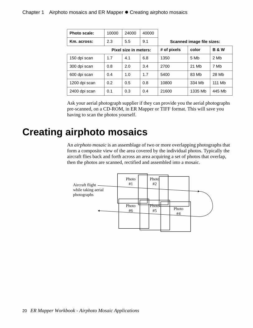
Use the following table to decide what scale aerial photography to use and wDPI resolution to use when scanning the photos. A pixel size of 1 meter is adequate for many applications.
ER Mapper Workbook - Airphoto Mosaic Applications 19
Chapter 1#Airphoto mosaics and ER Mapper z Creating airphoto mosaics
aphs
that the lap,
Ask your aerial photograph supplier if they can provide you the aerial photogrpre-scanned, on a CD-ROM, in ER Mapper or TIFF format. This will save youhaving to scan the photos yourself.
Creating airphoto mosaicsAn airphoto mosaic is an assemblage of two or more overlapping photographs form a composite view of the area covered by the individual photos. Typicallyaircraft flies back and forth across an area acquiring a set of photos that overthen the photos are scanned, rectified and assembled into a mosaic.
Photo scale: 10000 24000 40000
Km. across: 2.3 5.5 9.1
# of pixels color B & W
150 dpi scan 1.7 4.1 6.8 1350 5 Mb 2 Mb
300 dpi scan 0.8 2.0 3.4 2700 21 Mb 7 Mb
600 dpi scan 0.4 1.0 1.7 5400 83 Mb 28 Mb
1200 dpi scan 0.2 0.5 0.8 10800 334 Mb 111 Mb
2400 dpi scan 0.1 0.3 0.4 21600 1335 Mb 445 Mb
Aircraft flightwhile taking aerialphotographs
Photo#1
Photo#2
Photo#4
Photo#5
Photo#6
Scanned image file sizes:
Pixel size in meters:
20 ER Mapper Workbook - Airphoto Mosaic Applications
Chapter 1#Airphoto mosaics and ER Mapper#z Creating airphoto mosaics
hese
s
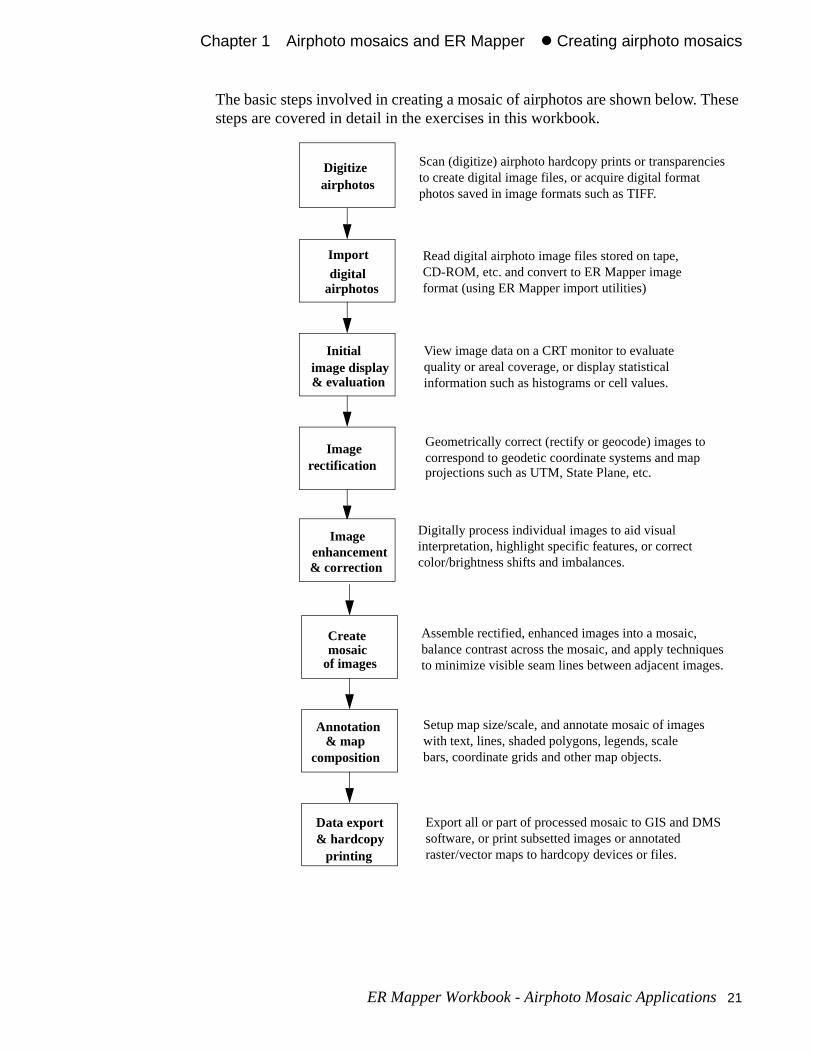
The basic steps involved in creating a mosaic of airphotos are shown below. Tsteps are covered in detail in the exercises in this workbook.
Digitize
Import
Initial
Image
Image
Scan (digitize) airphoto hardcopy prints or transparencies
Digitally process individual images to aid visual
airphotos
digital
image display& evaluation
rectification
enhancement
Create
Annotation
Data export
mosaicof images
& mapcomposition
& hardcopyprinting
to create digital image files, or acquire digital formatphotos saved in image formats such as TIFF.
interpretation, highlight specific features, or correct color/brightness shifts and imbalances.
Assemble rectified, enhanced images into a mosaic,
Setup map size/scale, and annotate mosaic of images
Export all or part of processed mosaic to GIS and DMS
balance contrast across the mosaic, and apply techniqueto minimize visible seam lines between adjacent images.
with text, lines, shaded polygons, legends, scalebars, coordinate grids and other map objects.
software, or print subsetted images or annotatedraster/vector maps to hardcopy devices or files.
airphotos
Read digital airphoto image files stored on tape,CD-ROM, etc. and convert to ER Mapper imageformat (using ER Mapper import utilities)
View image data on a CRT monitor to evaluatequality or areal coverage, or display statisticalinformation such as histograms or cell values.
Geometrically correct (rectify or geocode) images to correspond to geodetic coordinate systems and mapprojections such as UTM, State Plane, etc.
& correction
ER Mapper Workbook - Airphoto Mosaic Applications 21
Chapter 1#Airphoto mosaics and ER Mapper z Creating airphoto mosaics
use M, nto
r sing tes
BIL)
tion for s), or lpful r
he
ing
CRT ge of ality,
or
os or
of a
Data import
The first step in creating an airphoto mosaic is importing the data you want tointo ER Mapper. Typically the data might be stored on magnetic tape, CD-ROor other media. There are two primary types of data you may want to import iER Mapper: raster and vector.
Raster image data is the type used as input to image processing operations, foexample a digitized aerial photograph. When you import a raster image file (uER Mapper’s import utility programs), ER Mapper converts the data and creatwo files:
• a binary data file containing the image data, in band interleaved by line (format
• a corresponding ASCII header file with an “.ers” file extension
Vector data is stored as lines, points, and polygons. Many geographic informasystem (GIS) products use vector data structures because it is more efficientrepresenting discrete spatial objects like roads (lines), sample locations (pointpolitical boundaries (polygons). In an image processing product, it is often heto use vector data as a source of ground control for rectifying raw airphotos, ooverlaying vector data on top of a raster image backdrop. When you import avector file (using ER Mapper’s import utility programs), ER Mapper converts tdata and creates two files:
• an ASCII data file containing the vector data
• a corresponding ASCII header file with an “.erv” file extension
Note: You can open image files in many different formats in ER Mapper without havto import them as ER Mapper raster datasets.
Image display
After importing the data, the next step is usually to display the image on your monitor to evaluate the data quality, geographic area of coverage, and coveraoverlapping areas with other images used in a mosaic. If the data is of poor quyou might decide to digitize the photos again. If it has significant cloud cover haze over your area of interest, you might try to obtain better data.
There are two primary ways airphotos are viewed:
• black and white, or greyscale, displays (used to view black and white airphota single band of a color airphoto)
• red-green-blue (RGB) color composite displays (used to view all three bandscolor or color IR airphoto to reproduce the look of the original print)
22 ER Mapper Workbook - Airphoto Mosaic Applications
Chapter 1#Airphoto mosaics and ER Mapper#z Creating airphoto mosaics
uch
view
les.
etric quired, r
ow
titude/
s, and
do
tract
”
e
The way in which you choose to display your raster data is called the “Color Mode” in ER Mapper. You can also view data in traditional two-dimensional planimetric views, or 3-D perspective views if you have an elevation dataset sas a DTM.
In addition to displaying the data, you may want to view statistical informationabout it. Statistics are often good indicators of image quality. You may want tocalculate statistics for the image, such as the mean value in each band, and them in a tabular format. Or you may want to view statistical information in a graphical format using tools like histograms, scattergrams, and traverse profi
Image geocodingMany times, raster image data is supplied in a “raw” state and contains geomerrors. Whenever accurate area, direction, and distance measurements are reraw image data must usually be processed to remove geometric errors and/orectify the image to a real world coordinate system.
• Registration is the process of geometrically aligning two or more images to allthem to be superimposed or overlaid.
• Rectification is the process of geometrically correcting raster images so they correspond to real world map projections and coordinate systems (such as LaLongitude or Eastings/Northings).
• Orthorectification is a more accurate form of rectification mainly used on airphotos. It takes into account properties of the camera used to take the imagefiducial marks on the image.
If your application requires that your images be registered to one another or rectified to a map projection, you will use ER Mapper’s Geocoding Wizard to this.
Image enhancement and correction
Image enhancement refers to any one of many types of image processing operations used to digitally process image data to aid visual interpretation, exquantitative information, or correct color/brightness distortions. Image enhancement is what many people commonly think of as “image processing.
In ER Mapper, image enhancement operations are greatly simplified by the “algorithms” processing concept. Nearly all types of image enhancement operations can be applied and displayed in real time to provide truly interactivcontrol without writing temporary files to disk.
Typical image enhancement operations include:
ER Mapper Workbook - Airphoto Mosaic Applications 23
Chapter 1#Airphoto mosaics and ER Mapper z Creating airphoto mosaics
ast. Or,
tic. An
with
ar orhance
aidctral
etail.
yrain/ation.
a
renced
te rder rking ile.
bular d in ucts.
• Contrast enhancements–Improve image presentation by maximizing the contrbetween light and dark portions (or high and low data values) in an imagehighlight a specific data range or spatial area in an image.
• Formula processing–Apply mathematical operations to derive specific themainformation or correct/normalize color and brightness shifts across an imageexample would be the color balancing formulas to correct color shifts suppliedER Mapper.
• Filtering–Enhance edges, smooth noise, or highlight or suppress specific linespatial features in images. For example, apply edge enhancement filters to endetail (sharpen) the image or smoothing filters to reduce noise.
• Image merging (data fusion)–Combine images with different qualities to interpretation. For example, merge a black and white airphoto with a multispesatellite image to combine satellite spectral information with airphoto spatial d
• 3-D perspective visualization–Create realistic 3-D perspective views simply badding a “height” element to the airphoto image display, such as digital terelevation data or any other type of data that may aid visualization and interpret
• Color balancing–Use the ER Mapper Color Balancing Wizard to balance mosaiced images to produce a seamless single image.
Creating image mosaics
A mosaic is an assemblage of two or more overlapping images used to createcontinuous representation of the area covered by the images. ER Mapper automates the building of image mosaics because co-registered images refein the same processing algorithm are automatically displayed in their correct geographic positions relative to each other.
This means that you can work with each image file in the mosaic as a separaentity, and you are not required to write all images to one large file on disk in oto process and enhance them. This capability is especially important when wowith large image files such as scanned airphotos, because final mosaics canconsume gigabytes of disk space if they would have to be saved in a single f
The ER Mapper Image Display and Mosaic Wizard automatically mosiacs images in a specified directory path.
Map composition
You can use ER Mapper’s built-in Annotation and Map Composition tools to create top quality maps combining airphoto images or mosaics, vector, and tadata. Annotation lets you draw directly on-screen using text, line, polygon, another annotation tools, and specify fill color, shading, line styles, user-definedsymbols, and group, move and resize objects. Vector annotation files createdER Mapper can also be exported to external file formats for use in other prod
24 ER Mapper Workbook - Airphoto Mosaic Applications
Chapter 1#Airphoto mosaics and ER Mapper#z Image processing concepts
y many
pose ut as ily
te erent tive
or use
use inppingmatic
essed
, andaphicsringn any
int
ript,
ful to
lled he
ER Mapper’s Map Composition tools let you create top quality image maps badding coordinate grids, map collars, scale bars, legends, north arrows, and other map objects and standard cartographic symbols. You can layout and commaps comprised of multiple processed images, and size and scale map outpdesired. All map objects are defined as full color PostScript, and you can easadd custom map objects such as company logos or special north arrows.
Data export and hardcopy
Once you have completed processing your data, ER Mapper lets you translaraster and vector data to external standard file formats or print to over 200 diffhardcopy devices. You can easily print both 2-D planimetric and 3-D perspecviews.
• ECW Compression enables you to save your imagery in compressed format fin other applications.
• Data export is used to export all or part of a processed airphoto mosaic for other software products, such as a backdrop for a GIS or DMS (desktop masystem) product. Or, you may want export vector annotation or vectorized thedata to a GIS product.
• Free plug-ins enable you to open ER Mapper images, including ECW comprimages, from within many GIS products.
• Hardcopy printing is often the final goal of processing and annotating imagesER Mapper provides unsurpassed hardcopy support and output to standard grfile formats. ER Mapper also includes a built-in PostScript-compatible rendeengine, so you get PostScript-quality output (such as beautiful, smooth text) osupported device, whether the device supports PostScript or not.
You can also easily print at exact sizes and map scales, and automatically prlarge images in strips for assembling a mosaic of prints. Supported hardcopydevices include inkjet printers, laser printers, dye sublimation printers, electrostatic plotters, and film recorders. Graphics file formats include PostScTIFF, Targa, CGM, and CMYK and RGB color separations.
Image processing conceptsThe term digital image processing refers to the use of a computer to manipulateimage data stored in a digital format. The goal of image processing for earth science applications is to enhance geographic data to make it more meaningthe user, extract quantitative information, and solve problems.
A digital image is stored as a two-dimensional array (or grid) of small areas capixels (picture elements), and each pixel corresponds spatially to an area on tearth’s surface. This array or grid structure is also called a raster, so image data is
ER Mapper Workbook - Airphoto Mosaic Applications 25
Chapter 1#Airphoto mosaics and ER Mapper z Traditional image processing
n ld be
ange
o,
960’s ed the
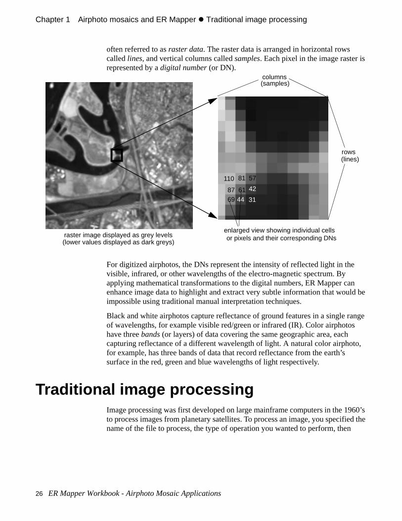
often referred to as raster data. The raster data is arranged in horizontal rows called lines, and vertical columns called samples. Each pixel in the image raster isrepresented by a digital number (or DN).
For digitized airphotos, the DNs represent the intensity of reflected light in thevisible, infrared, or other wavelengths of the electro-magnetic spectrum. By applying mathematical transformations to the digital numbers, ER Mapper caenhance image data to highlight and extract very subtle information that wouimpossible using traditional manual interpretation techniques.
Black and white airphotos capture reflectance of ground features in a single rof wavelengths, for example visible red/green or infrared (IR). Color airphotoshave three bands (or layers) of data covering the same geographic area, each capturing reflectance of a different wavelength of light. A natural color airphotfor example, has three bands of data that record reflectance from the earth’s surface in the red, green and blue wavelengths of light respectively.
Traditional image processingImage processing was first developed on large mainframe computers in the 1to process images from planetary satellites. To process an image, you specifiname of the file to process, the type of operation you wanted to perform, then
rows(lines)
columns(samples)
raster image displayed as grey levels(lower values displayed as dark greys)
enlarged view showing individual cellsor pixels and their corresponding DNs
61
110 81 57
87
69 44
42
31
26 ER Mapper Workbook - Airphoto Mosaic Applications
Chapter 1#Airphoto mosaics and ER Mapper#z ER Mapper image processing
e file am to
ge e
sing disk ults.
isk
, the g a
r ssing
ta,
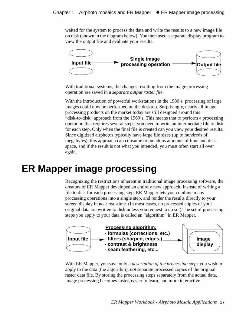
waited for the system to process the data and write the results to a new imagon disk (shown in the diagram below). You then used a separate display progrview the output file and evaluate your results.
With traditional systems, the changes resulting from the image processing operation are saved in a separate output raster file.
With the introduction of powerful workstations in the 1980’s, processing of larimages could now be performed on the desktop. Surprisingly, nearly all imagprocessing products on the market today are still designed around this “disk-to-disk” approach from the 1960’s. This means that to perform a procesoperation that requires several steps, you need to write an intermediate file tofor each step. Only when the final file is created can you view your desired resSince digitized airphotos typically have large file sizes (up to hundreds of megabytes), this approach can consume tremendous amounts of time and dspace, and if the result is not what you intended, you must often start all overagain.
ER Mapper image processingRecognizing the restrictions inherent in traditional image processing softwarecreators of ER Mapper developed an entirely new approach. Instead of writinfile to disk for each processing step, ER Mapper lets you combine many processing operations into a single step, and render the results directly to youscreen display in near real-time. (In most cases, no processed copies of youroriginal data are written to disk unless you request to do so.) The set of procesteps you apply to your data is called an “algorithm” in ER Mapper.
With ER Mapper, you save only a description of the processing steps you wish to apply to the data (the algorithm), not separate processed copies of the original raster data file. By storing the processing steps separately from the actual daimage processing becomes faster, easier to learn, and more interactive.
Input fileSingle image
processing operation Output file
Processing algorithm: - formulas (corrections, etc.)
Input file - filters (sharpen, edges,) - contrast & brightness - seam feathering, etc...
Imagedisplay
ER Mapper Workbook - Airphoto Mosaic Applications 27

Chapter 1#Airphoto mosaics and ER Mapper z ER Mapper image processing
of ctive
hoto s.
ortant
In ER Mapper, algorithms can be used for simple viewing of data such as greyscale or RGB band combinations. Algorithms are also used for complex processing and modelling operations involving many images, transformationsthe data, and overlays of vector data–in both 2-D planimetric and 3-D perspeviews.
The algorithms design also allows ER Mapper to easily handle very large airpimages (and mosaics of images) much more efficiently than traditional systemReducing the need to write processed copies of the data to disk is a very impconsideration.
28 ER Mapper Workbook - Airphoto Mosaic Applications
ce. It and
r
site.
er’s ing The
2
User interfacebasics
This chapter introduces the basic use of the ER Mapper graphical user interfagives you practice using menus, toolbars, dialog boxes, and image windows,loading and displaying image processing algorithms.
Note: In order to complete the exercises in this manual, you will need to access theexample images and algorithms supplied with ER Mapper. If needed, ask yousystem manager for the location of the ER Mapper software directory at your
User interface componentsThis section provides a brief introduction to the main components of ER Mappgraphical user interface (GUI). You can perform nearly all operations by pointand clicking with the mouse, and very little typing on the keyboard is required. GUI is part of ER Mapper’s original design, so it is well integrated and easy tolearn and use.
ER Mapper Workbook - Airphoto Mosaic Applications 29
Chapter 2#User interface basics#z User interface components
ions
n nual
se
se
Using mouse buttonsWhen using ER Mapper, use the left button on your mouse to perform operatlike selecting items from menus, manipulating image windows, and drawing annotation. In this manual, all actions are performed with the left mouse buttounless otherwise indicated. The following table explains terms used in this mato describe actions you perform with the mouse.
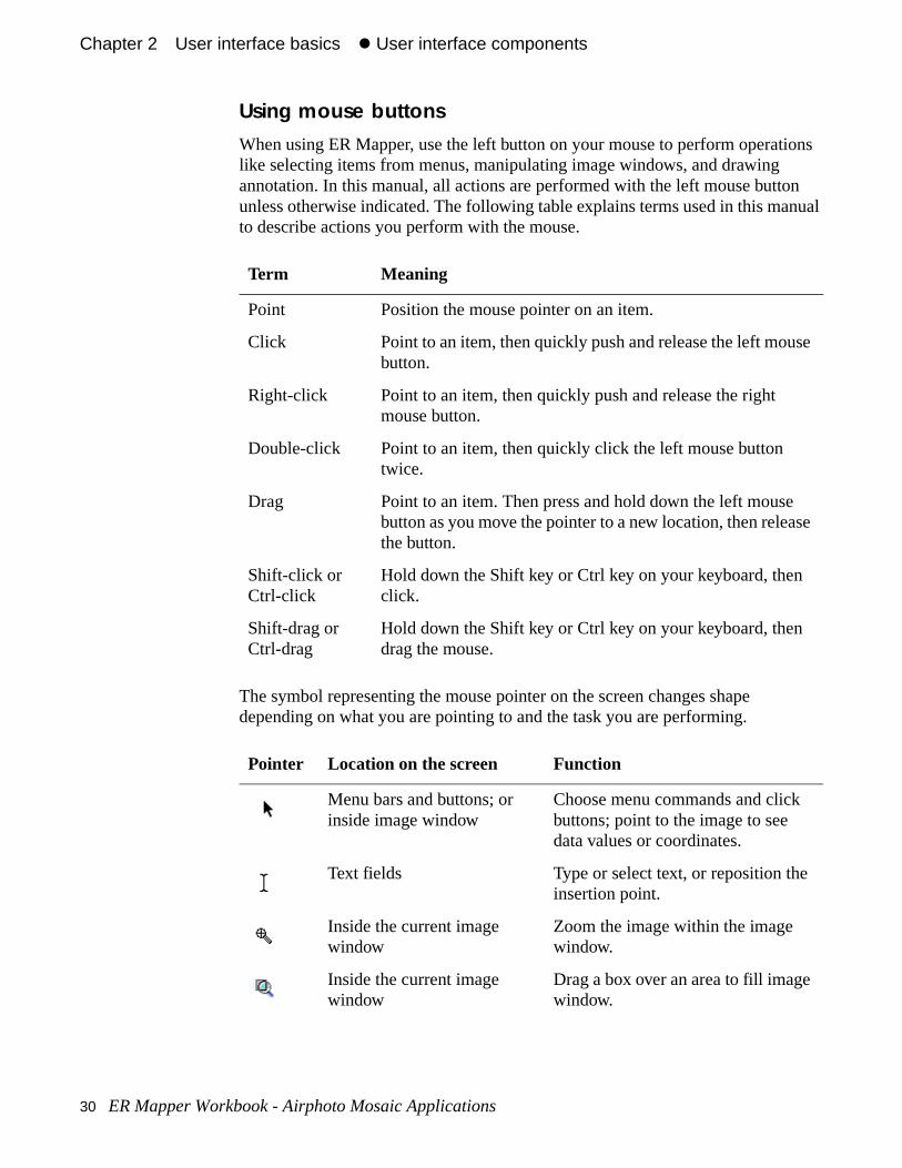
The symbol representing the mouse pointer on the screen changes shape depending on what you are pointing to and the task you are performing.
Term Meaning
Point Position the mouse pointer on an item.
Click Point to an item, then quickly push and release the left moubutton.
Right-click Point to an item, then quickly push and release the right mouse button.
Double-click Point to an item, then quickly click the left mouse button twice.
Drag Point to an item. Then press and hold down the left mousebutton as you move the pointer to a new location, then releathe button.
Shift-click orCtrl-click
Hold down the Shift key or Ctrl key on your keyboard, then click.
Shift-drag or Ctrl-drag
Hold down the Shift key or Ctrl key on your keyboard, then drag the mouse.
Pointer Location on the screen Function
Menu bars and buttons; or inside image window
Choose menu commands and click buttons; point to the image to see data values or coordinates.
Text fields Type or select text, or reposition theinsertion point.
Inside the current image window
Zoom the image within the image window.
Inside the current image window
Drag a box over an area to fill image window.
30 ER Mapper Workbook - Airphoto Mosaic Applications
Chapter 2#User interface basics#z User interface components
n e or
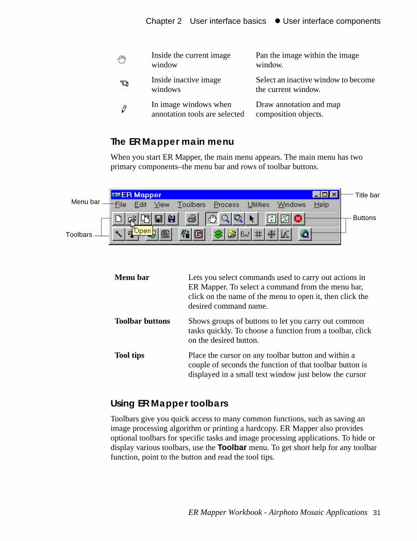
The ER Mapper main menuWhen you start ER Mapper, the main menu appears. The main menu has twoprimary components–the menu bar and rows of toolbar buttons.
Using ER Mapper toolbarsToolbars give you quick access to many common functions, such as saving aimage processing algorithm or printing a hardcopy. ER Mapper also providesoptional toolbars for specific tasks and image processing applications. To hiddisplay various toolbars, use the Toolbar menu. To get short help for any toolbarfunction, point to the button and read the tool tips.
Inside the current image window
Pan the image within the image window.
Inside inactive image windows
Select an inactive window to becomethe current window.
In image windows when annotation tools are selected
Draw annotation and map composition objects.
Menu bar Lets you select commands used to carry out actions in ER Mapper. To select a command from the menu bar, click on the name of the menu to open it, then click the desired command name.
Toolbar buttons Shows groups of buttons to let you carry out common tasks quickly. To choose a function from a toolbar, clickon the desired button.
Tool tips Place the cursor on any toolbar button and within a couple of seconds the function of that toolbar button is displayed in a small text window just below the cursor
Title bar
Buttons
Toolbars
Menu bar
ER Mapper Workbook - Airphoto Mosaic Applications 31
Chapter 2#User interface basics#z User interface components
s ard,
ized tom
e
u
ral r
e
ER Mapper provides toolbars for many common tasks, and also toolbars for building processing algorithms commonly used in remote sensing applicationsuch as forestry, geophysics, and map generation. The functions of the Standand Common Functions toolbars are summarized below.
Using ER Mapper’s scripting language, you can also create your own customtoolbars for specific tasks and functions. For more information on creating custoolbars, see the ER Mapper User Guide.
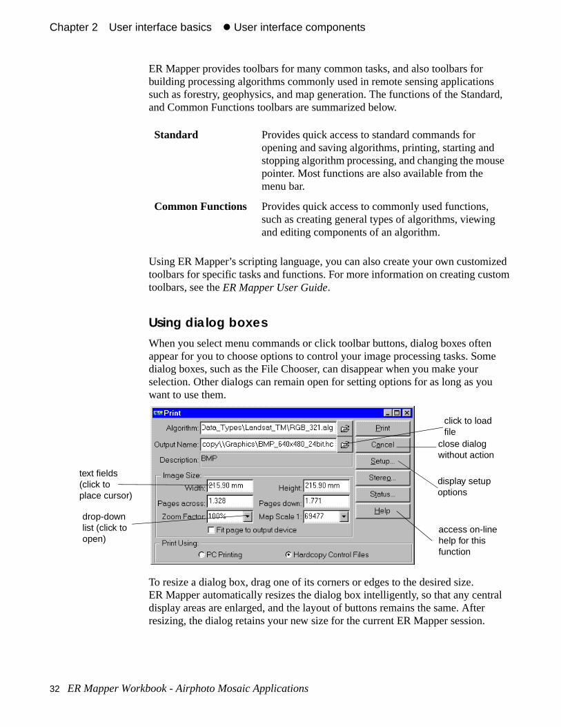
Using dialog boxesWhen you select menu commands or click toolbar buttons, dialog boxes oftenappear for you to choose options to control your image processing tasks. Somdialog boxes, such as the File Chooser, can disappear when you make your selection. Other dialogs can remain open for setting options for as long as yowant to use them.
To resize a dialog box, drag one of its corners or edges to the desired size. ER Mapper automatically resizes the dialog box intelligently, so that any centdisplay areas are enlarged, and the layout of buttons remains the same. Afteresizing, the dialog retains your new size for the current ER Mapper session.
Standard Provides quick access to standard commands for opening and saving algorithms, printing, starting and stopping algorithm processing, and changing the mouspointer. Most functions are also available from the menu bar.
Common Functions Provides quick access to commonly used functions, such as creating general types of algorithms, viewing and editing components of an algorithm.
text fields(click toplace cursor)
drop-downlist (click toopen)
click to loadfile
close dialogwithout action
display setupoptions
access on-linehelp for thisfunction
32 ER Mapper Workbook - Airphoto Mosaic Applications
Chapter 2#User interface basics#z User interface components
per
k
r
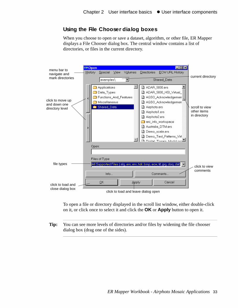
Using the File Chooser dialog boxesWhen you choose to open or save a dataset, algorithm, or other file, ER Mapdisplays a File Chooser dialog box. The central window contains a list of directories, or files in the current directory.
To open a file or directory displayed in the scroll list window, either double-clicon it, or click once to select it and click the OK or Apply button to open it.
Tip: You can see more levels of directories and/or files by widening the file choosedialog box (drag one of the sides).
current directory
scroll to view other itemsin directory
click to viewcomments
click to load and leave dialog open
click to load andclose dialog box
click to move upand down onedirectory level
menu bar to navigate andmark directories
file types
ER Mapper Workbook - Airphoto Mosaic Applications 33
Chapter 2#User interface basics#z User interface components
iews
to an sor.
k on
.
r
of
The File Chooser menus at the top have the following functions:
Using the on-line help systemER Mapper provides an extensive on-line help system with both simple overvand detailed descriptions of all features and functions. There are two ways toaccess help:
Typing text in text fieldsTo enter text for naming files or changing values in dialog boxes, ER Mapper provides text fields. When you point to a text field, the pointer shape changes I-beam. To enter text, click anywhere inside the text field to place the text cur
To select existing text, you can drag through the desired portion, or double-clica word or numeric value to select it. Text that is selected become reverse highlighted, and any subsequent typing replaces it.
History menu Use to change the File Chooser’s current directoryThe menu has two parts: the upper portion lists most recently visited directories, and the lower portion lists marked directories.
Special menu Use to change to your home directory, or to mark ounmark a directory (any directory may be marked for fast access using the History menu).
View menu Use to sort the contents of the current directory byname, date modified, or date created.
Volumes menu (Windows version only)
Use to access volumes or disk drives on your network.
Directories menu Use to change to any directory defined by your preferences settings.
ECW URL History List of the most recent ECW Compressed image files accessed via an Image Web Server by means their URLs.
Help menu Lets you browse all the standard ER Mapper manuals on-line, and go between manuals and topics using hypertext links.
Help buttons The Help button inside dialog boxes gives you context-sensitive help. If needed, you can navigateto view more detailed information using the hypertext links.
34 ER Mapper Workbook - Airphoto Mosaic Applications
Chapter 2#User interface basics#z Hands-on exercises
g
e
-line
Hands-on exercisesThe following hands-on exercises introduce you to the basic concepts of usinmenus and dialog boxes and managing image windows.
• Choose options from menus and toolbar buttons
• Display and hide toolbars
• Open an empty image window
• Open an image processing algorithm into a window
• Move and resize an image window
• Zoom and pan the image within the window
• Manipulate multiple image windows on the screen
• Close image windows
1: Using menus and toolbars
Move the ER Mapper main menu around the screen1 Position the mouse pointer on the ER Mapper main menu title bar, then
drag it to the lower-left part of the screen.
Pointing to the title bar and dragging is how you move dialog boxes and imagwindows around the screen.
2 Drag the main menu to the upper-right corner of the screen.
This is the recommended position for the main menu for the exercises in this tutorial.
What you will learn...
After completing these exercises, you will know how to perform the following tasks in ER Mapper:
Objectives Learn to open and make selections from menus, use toolbars, and access onhelp.
ER Mapper Workbook - Airphoto Mosaic Applications 35
Chapter 2#User interface basics#z 1: Using menus and toolbars
lows:
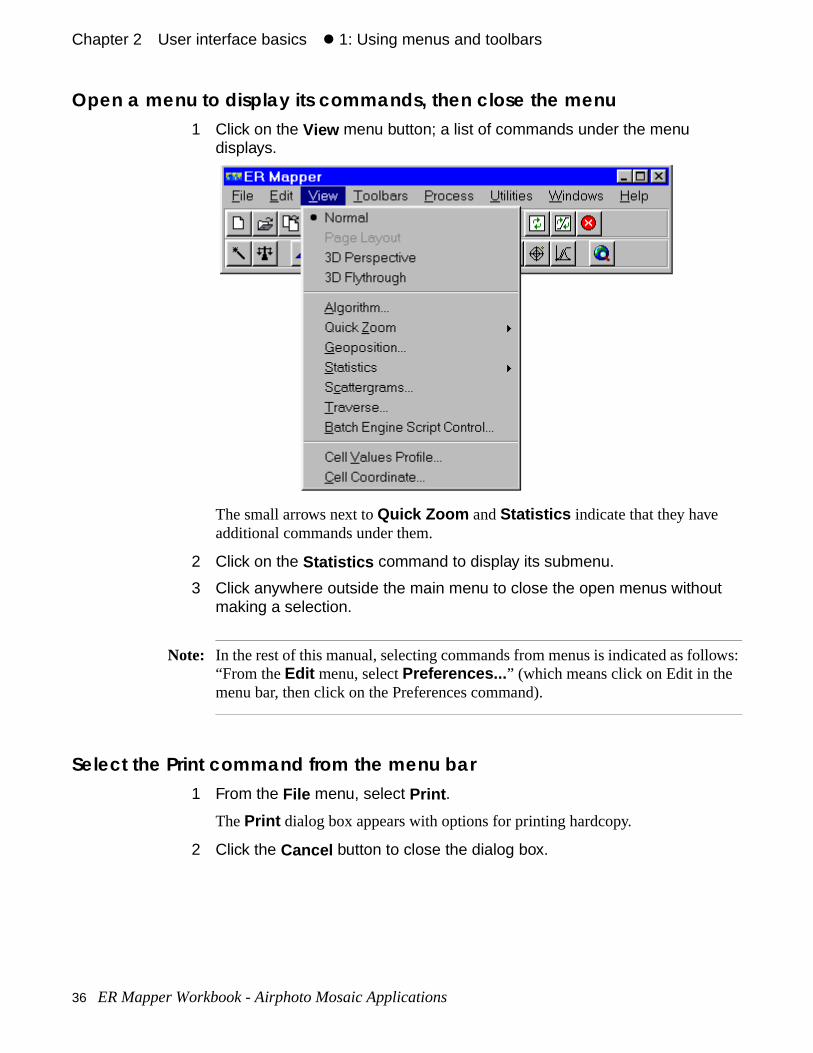
Open a menu to display its commands, then close the menu1 Click on the View menu button; a list of commands under the menu
displays.
The small arrows next to Quick Zoom and Statistics indicate that they have additional commands under them.
2 Click on the Statistics command to display its submenu.
3 Click anywhere outside the main menu to close the open menus without making a selection.
Note: In the rest of this manual, selecting commands from menus is indicated as fol“From the Edit menu, select Preferences... ” (which means click on Edit in the menu bar, then click on the Preferences command).
Select the Print command from the menu bar1 From the File menu, select Print .
The Print dialog box appears with options for printing hardcopy.
2 Click the Cancel button to close the dialog box.
36 ER Mapper Workbook - Airphoto Mosaic Applications
Chapter 2#User interface basics#z 1: Using menus and toolbars
ter
on the
and
he
lay
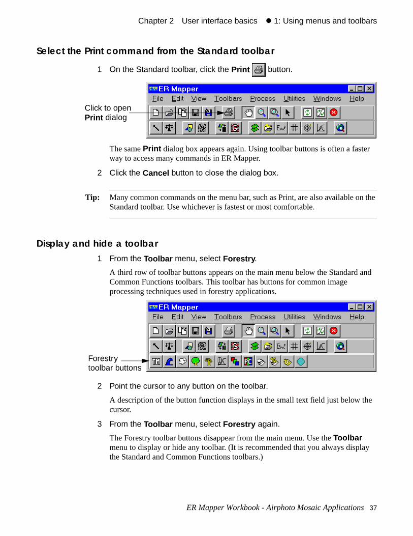
Select the Print command from the Standard toolbar
1 On the Standard toolbar, click the Print button.
The same Print dialog box appears again. Using toolbar buttons is often a fasway to access many commands in ER Mapper.
2 Click the Cancel button to close the dialog box.
Tip: Many common commands on the menu bar, such as Print, are also available Standard toolbar. Use whichever is fastest or most comfortable.
Display and hide a toolbar1 From the Toolbar menu, select Forestry .
A third row of toolbar buttons appears on the main menu below the Standard Common Functions toolbars. This toolbar has buttons for common image processing techniques used in forestry applications.
2 Point the cursor to any button on the toolbar.
A description of the button function displays in the small text field just below tcursor.
3 From the Toolbar menu, select Forestry again.
The Forestry toolbar buttons disappear from the main menu. Use the Toolbar menu to display or hide any toolbar. (It is recommended that you always dispthe Standard and Common Functions toolbars.)
Click to openPrint dialog
Forestrytoolbar buttons
ER Mapper Workbook - Airphoto Mosaic Applications 37
Chapter 2#User interface basics#z 2: Opening windows and algorithms
en raster ender ou
dow
of 2, the
that
n
2: Opening windows and algorithmsTo display an image in ER Mapper, you first open an empty image window, thload and display an image processing algorithm. The algorithm references a data file on disk, and the processing steps ER Mapper uses to enhance and rthe data on the screen display. (You will learn more about algorithms later.) Ycan have as many different image windows open on the screen as you need.
Open a new empty image window1 From the File menu, select New.
An empty image window opens in the upper left corner of the screen. The wintitle bar reads “Algorithm Not Yet Saved” because no processing algorithm is associated with this image window yet.
Open and display an image processing algorithm1 From the File menu, select Open... .
The Open file chooser dialog box opens.
2 From the Directories menu, select the path ending with the text \examples (The portion of the path name preceding it is specific to your site.)
3 Double-click on the directory named ‘Data_Types’ to open it.
4 Double-click on the directory named ‘Landsat_TM’ to open it. (Scroll if needed to view it first.)
The list of example algorithms for processing Landsat Thematic Mapper (TM)satellite imagery displays.
5 Double-click on the algorithm named ‘RGB_321.alg.’ (Scroll down if needed to view it first.)
ER Mapper runs the algorithm and displays an enhanced Landsat TM image San Diego, California in the image window. This algorithm displays bands 3, and 1 of the Landsat image as an RGB color composite image, with band 3 inred display channel, band 2 in the green, and band 1 in the blue. Notice alsothe algorithm filename ‘RGB_321’ now appears in the title bar of the image window.
Objectives Learn to open image windows on your computer display, and open and run aimage processing algorithm stored on disk.
38 ER Mapper Workbook - Airphoto Mosaic Applications
Chapter 2#User interface basics#z 3: Resizing windows and zooming/panning
ndsat s to
n it
und
and
Use the toolbar to open a different processing algorithm
1 Click the Open button on the Standard toolbar.
The Open file chooser dialog box appears. (This toolbar button has the samefunction as selecting Open... from the File menu.)
The algorithm named ‘RGB_321’ in the ‘Data_Types\Landsat_TM’ directory isalready highlighted since it is currently loaded into the image window.
2 Double-click on the algorithm named ‘RGB_541.alg.’
ER Mapper runs the algorithm and displays a color composite of the same Laimage, this time using bands 5, 4, and 1. Notice that the title bar also changeshow the filename of the new algorithm.
Note: By default, ER Mapper runs the algorithm automatically for you when you opefrom disk. You can also reprocess the data at any time by clicking the Refresh
button.
3: Resizing windows and zooming/panning
Move the image window on the screen1 Point the mouse at the image window title bar, then drag it to another part
of the screen.
2 Drag the image back to the upper-left part of the screen.
Like dialog boxes, dragging images by the title bar is how you move them arothe screen.
Resize the image window1 Move the mouse pointer directly over the lower-right corner of the image
window–the pointer shape changes to a double ended arrow.
Objectives Learn to move and resize image windows, zoom (magnify) part of an image, pan (scroll) to other parts of an image.
ER Mapper Workbook - Airphoto Mosaic Applications 39
Chapter 2#User interface basics#z 3: Resizing windows and zooming/panning
the cate
ed
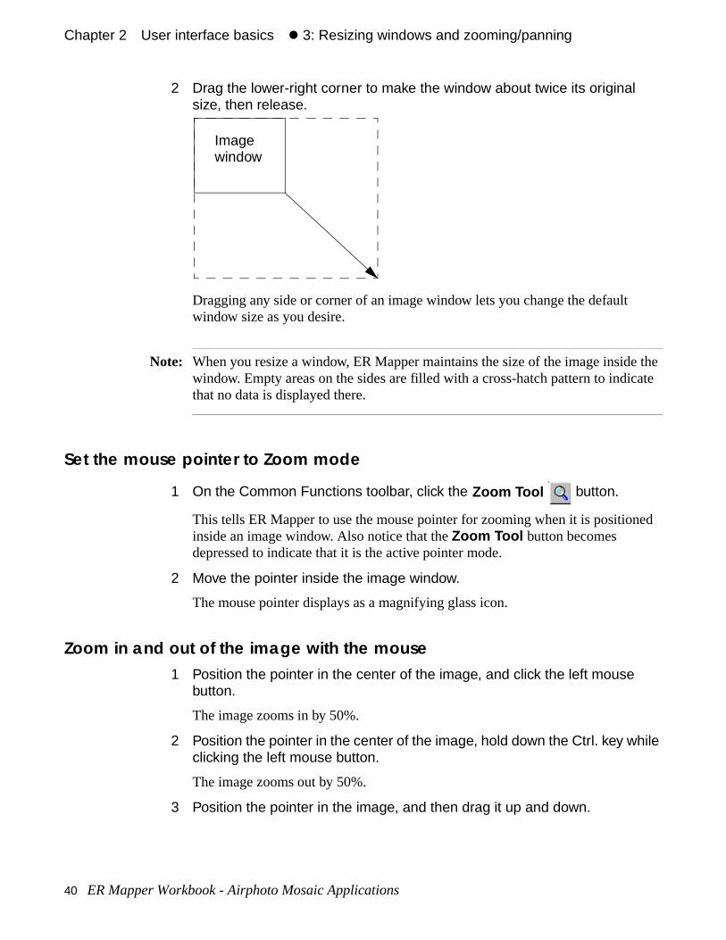
2 Drag the lower-right corner to make the window about twice its original size, then release.
Dragging any side or corner of an image window lets you change the default window size as you desire.
Note: When you resize a window, ER Mapper maintains the size of the image insidewindow. Empty areas on the sides are filled with a cross-hatch pattern to indithat no data is displayed there.
Set the mouse pointer to Zoom mode
1 On the Common Functions toolbar, click the Zoom Tool button.
This tells ER Mapper to use the mouse pointer for zooming when it is positioninside an image window. Also notice that the Zoom Tool button becomes depressed to indicate that it is the active pointer mode.
2 Move the pointer inside the image window.
The mouse pointer displays as a magnifying glass icon.
Zoom in and out of the image with the mouse1 Position the pointer in the center of the image, and click the left mouse
button.
The image zooms in by 50%.
2 Position the pointer in the center of the image, hold down the Ctrl. key while clicking the left mouse button.
The image zooms out by 50%.
3 Position the pointer in the image, and then drag it up and down.
Imagewindow
40 ER Mapper Workbook - Airphoto Mosaic Applications
Chapter 2#User interface basics#z 3: Resizing windows and zooming/panning
en
it is
ifies
ing
ed
As you drag the pointer down the image is magnified, i.e you zoom into it. Whyou drag the pointer upwards, the image gets smaller, i.e you zoom out.
Set the mouse pointer to ZoomBox mode
1 On the Common Functions toolbar, click the ZoomBox Tool button.
This tells ER Mapper to use the mouse pointer for creating a zoom box whenpositioned inside an image window. Also notice that the ZoomBox Tool button becomes depressed to indicate that it is the active pointer mode.
2 Move the pointer inside the image window.
The mouse pointer displays as a magnifying glass and box icon.
Zoom in (magnify) an area of the image with the mouse1 Position the pointer near the upper-left center of the image, then drag to the
lower-right to define a box.
When you release the mouse, ER Mapper runs the algorithm again and magn(or “zooms in”) on the area of the image you defined with the box. Dragging azoom box is a fast way to magnify an area of interest. (There are other zoomfunctions you will learn about later.
Set the mouse pointer to Hand mode
1 On the Common Functions toolbar, click the Hand Tool button.
This tells ER Mapper to use the mouse pointer for panning when it is positioninside an image window. Also notice that the Hand Tool button becomes depressed to indicate that it is the active pointer mode.
2 Move the pointer inside the image window.
The mouse pointer displays as a hand icon.
Pan (scroll) the image within the window with the mouse1 Click on the image. and drag it to a new position in the image window.
The hand pointer will grab the image and move it (pan) to the new location.
Zoom back out to view the full image extents1 From the View menu, select Quick Zoom and then select Zoom to All
Datasets .
ER Mapper Workbook - Airphoto Mosaic Applications 41
Chapter 2#User interface basics#z 3: Resizing windows and zooming/panning
tents r
ER Mapper runs the algorithm again and zooms back out to display the full exof the Landsat image data. The Quick Zoom submenu provides many options fozooming in or out to specific datasets, setting window geolinking, and other options you will learn more about later.
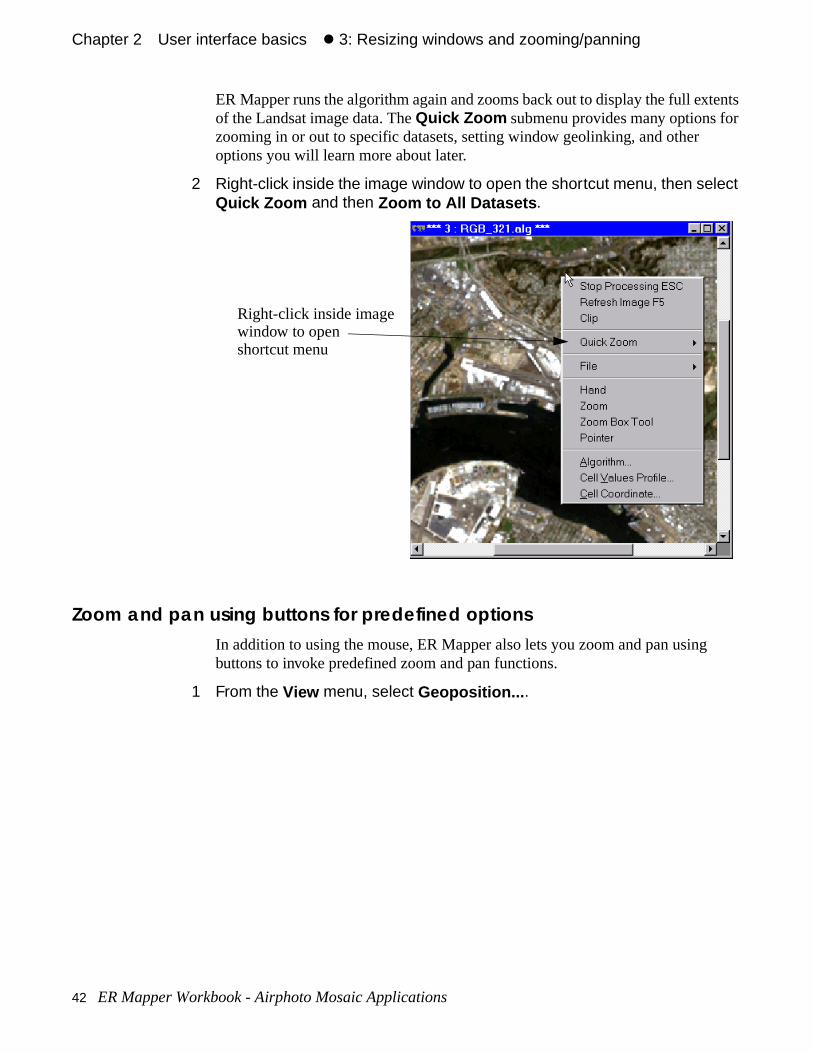
2 Right-click inside the image window to open the shortcut menu, then select Quick Zoom and then Zoom to All Datasets .
Zoom and pan using buttons for predefined optionsIn addition to using the mouse, ER Mapper also lets you zoom and pan usingbuttons to invoke predefined zoom and pan functions.
1 From the View menu, select Geoposition... .
Right-click inside imagewindow to open shortcut menu
42 ER Mapper Workbook - Airphoto Mosaic Applications
Chapter 2#User interface basics#z 3: Resizing windows and zooming/panning
ge
the age
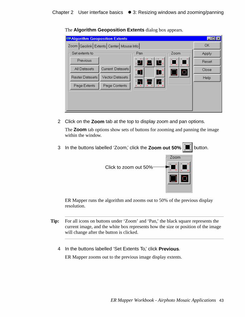
The Algorithm Geoposition Extents dialog box appears.
2 Click on the Zoom tab at the top to display zoom and pan options.
The Zoom tab options show sets of buttons for zooming and panning the imawithin the window.
3 In the buttons labelled ‘Zoom,’ click the Zoom out 50% button.
ER Mapper runs the algorithm and zooms out to 50% of the previous display resolution.
Tip: For all icons on buttons under ‘Zoom’ and ‘Pan,’ the black square represents current image, and the white box represents how the size or position of the imwill change after the button is clicked.
4 In the buttons labelled ‘Set Extents To,’ click Previous .
ER Mapper zooms out to the previous image display extents.
Click to zoom out 50%
ER Mapper Workbook - Airphoto Mosaic Applications 43
Chapter 2#User interface basics#z 4: Managing multiple image windows
nt is
is
dow.
s no
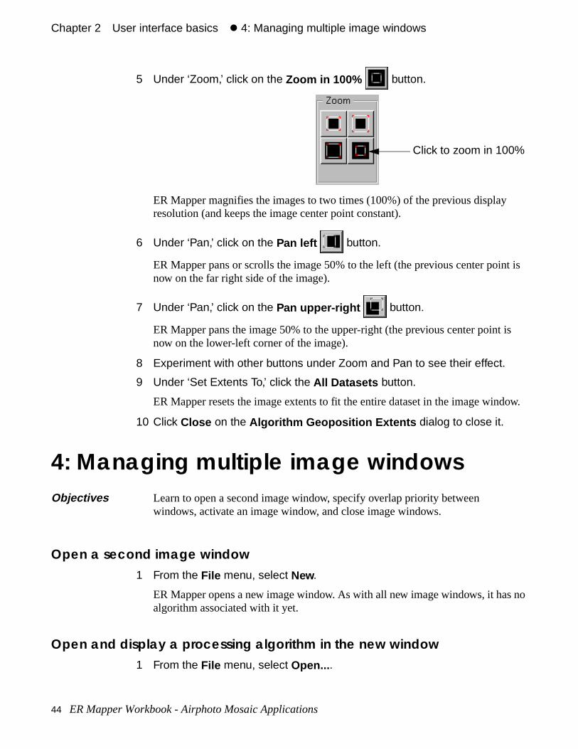
5 Under ‘Zoom,’ click on the Zoom in 100% button.
ER Mapper magnifies the images to two times (100%) of the previous displayresolution (and keeps the image center point constant).
6 Under ‘Pan,’ click on the Pan left button.
ER Mapper pans or scrolls the image 50% to the left (the previous center poinow on the far right side of the image).
7 Under ‘Pan,’ click on the Pan upper-right button.
ER Mapper pans the image 50% to the upper-right (the previous center pointnow on the lower-left corner of the image).
8 Experiment with other buttons under Zoom and Pan to see their effect.
9 Under ‘Set Extents To,’ click the All Datasets button.
ER Mapper resets the image extents to fit the entire dataset in the image win
10 Click Close on the Algorithm Geoposition Extents dialog to close it.
4: Managing multiple image windows
Open a second image window1 From the File menu, select New.
ER Mapper opens a new image window. As with all new image windows, it haalgorithm associated with it yet.
Open and display a processing algorithm in the new window1 From the File menu, select Open... .
Objectives Learn to open a second image window, specify overlap priority between windows, activate an image window, and close image windows.
Click to zoom in 100%
44 ER Mapper Workbook - Airphoto Mosaic Applications
Chapter 2#User interface basics#z 4: Managing multiple image windows
age e other t data,
ap.
e
The Open file chooser dialog box appears.
2 From the Directories menu, select the path ending with the text \examples .
3 Double-click on the directory named ‘Data_Types’ to open it.
4 Double-click on the directory named ‘SPOT_Panchromatic’ to open it.
The list of example algorithms for processing SPOT Panchromatic satellite imagery displays.
5 Double-click on the algorithm named ‘Greyscale.alg.’
ER Mapper runs the algorithm and displays a SPOT Panchromatic satellite imthe San Diego (the same geographic area covered by the Landsat image in thwindow). The SPOT Pan data provides greater spatial detail than the Landsabut has only one spectral band which is displayed in greyscale.
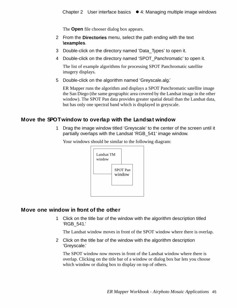
Move the SPOT window to overlap with the Landsat window1 Drag the image window titled ‘Greyscale’ to the center of the screen until it
partially overlaps with the Landsat ‘RGB_541’ image window.
Your windows should be similar to the following diagram:
Move one window in front of the other1 Click on the title bar of the window with the algorithm description titled
‘RGB_541.’
The Landsat window moves in front of the SPOT window where there is overl
2 Click on the title bar of the window with the algorithm description ‘Greyscale.’
The SPOT window now moves in front of the Landsat window where there is overlap. Clicking on the title bar of a window or dialog box bar lets you chooswhich window or dialog box to display on top of others.
Landsat TMwindow
SPOT Panwindow
ER Mapper Workbook - Airphoto Mosaic Applications 45
Chapter 2#User interface basics#z 4: Managing multiple image windows
s .
o.
move
.
in
in
Select a window to be the active windowThe “active” image window is the one you want to currently work with, such azooming, loading a new processing algorithm, or editing the current algorithm(You can have many image windows open on the screen, but only one can beactive.)
1 Look at the title bar of the SPOT Panchromatic window and notice the three asterisks (***) on either side of the window title.
The three asterisks indicate that this is the active (or current) window of the tw
2 Move the pointer inside the image area of the window with the algorithm description titled “RGB_541.”
The pointer shape changes to a pointing hand. (This happens whenever you from the active window to any inactive image window.)
3 Click anywhere inside the Landsat image window or on the Title Bar.
It now becomes the active window and three asterisks appear next to the title
4 Click inside the SPOT window or on the Title Bar again to make it active.
Note: A window can be active and still be covered by another “inactive” window. To move the active window to the front, click on its title bar.
Close both image windows1 Close one image window using the window system controls:
• For Windows, select Close from the window control-menu.
The window closes and disappears from the screen.
2 Close the other image window by repeating Step 1.
The window closes and disappears from the screen. Only the ER Mapper mamenu is now open.
• Choose options from menus and toolbar buttons
• Display and hide toolbars
• Open an empty image window
• Open an image processing algorithm into a window
• Move and resize an image window
What you learned
After completing these exercises, you know how to perform the following tasksER Mapper:
46 ER Mapper Workbook - Airphoto Mosaic Applications

Chapter 2#User interface basics#z 4: Managing multiple image windows
• Zoom and pan the image within the window
• Manipulate multiple image windows on the screen
• Close image windows
ER Mapper Workbook - Airphoto Mosaic Applications 47
Chapter 2#User interface basics#z 4: Managing multiple image windows
48 ER Mapper Workbook - Airphoto Mosaic Applications
u learn
new w to
splay. ve,
3
Importing andviewing an image
This chapter shows you how to import a digitized airphoto in TIFF format, andhow to display the dataset as a greyscale image and enhance the contrast. Yoabout the interface ER Mapper provides for creating and editing data view algorithms (the Algorithm dialog).
About the algorithms conceptThe goal of all image processing is to enhance your data to make it more meaningful and help you extract the type of information that interests you. Tomake this procedure faster and easier, Earth Resource Mapping developed aimage processing technique called “algorithm data views.” Understanding house algorithms is the key to understanding how to use ER Mapper effectively.
What is an algorithm data view?
An algorithm is a list of processing steps or instructions ER Mapper uses to transform raw datasets on disk into a final, enhanced image on your screen diIn this sense, algorithms let you define a “view” into your data that you can sareload, and modify at any time.
ER Mapper Workbook - Airphoto Mosaic Applications 49
Chapter 3#Importing and viewing an image#z About the algorithms concept
can
image
Hue
over
ge for
xity gain te
he
pes
pes oflayersions
epts. e to
You use ER Mapper’s graphical user interface to define your list of processingsteps, and you can save the steps in an algorithm file on disk. An algorithm filestore any of the following information about your processing:
• Names of dataset(s) to be processed and displayed
• Subsets of the dataset(s) to be processed (zoomed areas)
• Bands (layers of data) in the dataset(s) to be processed
• Color mapping and contrast enhancements (Transforms)
• Filtering to be applied to the data (Filters)
• Equations and combinations of bands or datasets used to create the (Formulae)
• Color mode used to display the data (Pseudocolor, Red Green Blue, orSaturation Intensity)
• Any vector datasets, thematic color, or map composition layers to be displayedthe raster image data
• Definition of a page size and margins (used for positioning the image on a pacreating maps and printing)
• Viewpoint and other parameters when viewing the image in 3D perspective
By being able to apply a set of processing steps as a single entity, the compleoften associated with image processing is greatly simplified. In addition, you tremendous savings in disk space, since you do not need to store intermediaprocessed copies of your original data on disk.
Building Algorithms in ER Mapper
There are three primary ways to build a processing algorithm in ER Mapper:
• Open a dataset directly (File Open ) and have ER Mapper automatically display tdataset using a simple default algorithm
• Use the Algorithm dialog options to build an algorithm by adding the desired tyof layers, loading datasets, and specify processing steps for each layer.
• Use image wizards to have ER Mapper automatically create any of several tyspecialized algorithms for you. In this case, ER Mapper adds the appropriate to the Algorithm dialog, prompts you to load a dataset, and possibly other optas well.
The majority of exercises in this workbook ask you to build algorithms from scratch so you become familiar with and thoroughly understand the basic concHowever, you will also use the automatic algorithm creation wizards from timtime to understand how they can save time.
50 ER Mapper Workbook - Airphoto Mosaic Applications
Chapter 3#Importing and viewing an image#z About the algorithms concept
n use asets. ce the
(color
y iques ing
.
Using Algorithms as Templates
Once you have saved your processing instructions as an algorithm file, you cathe algorithm as a “template” to easily apply the same processing to other datTo use an algorithm as a template, simply load the desired dataset(s) to repladefault dataset(s) saved with the algorithm, and click GO to apply the same processing to the new dataset(s). You may also need to adjust the transformsmapping) for the new datasets.
Any algorithm can be used as a template, and ER Mapper also provides mantemplate algorithms for common tasks. These include common display techn(pseudocolor, colordrape, etc.), writing processed image files to disk, and savalgorithms as “Virtual Datasets.”
The Algorithm dialog
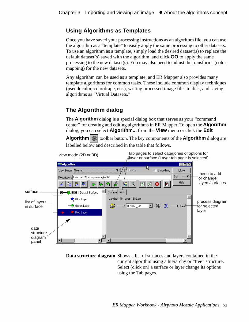
The Algorithm dialog is a special dialog box that serves as your “command center” for creating and editing algorithms in ER Mapper. To open the Algorithm dialog, you can select Algorithm... from the View menu or click the Edit
Algorithm toolbar button. The key components of the Algorithm dialog are
labelled below and described in the table that follows.
Data structure diagram Shows a list of surfaces and layers contained in the current algorithm using a hierarchy or “tree” structureSelect (click on) a surface or layer change its optionsusing the Tab pages.
process diagramfor selectedlayer
menu to addor changelayers/surfaces
tab pages to select categories of options forlayer or surface (Layer tab page is selected)
datastructurediagram
list of layersin surface
view mode (2D or 3D)
surface
panel
ER Mapper Workbook - Airphoto Mosaic Applications 51
Chapter 3#Importing and viewing an image#z About the algorithms concept
ne e en
at
en
er
y, essed,
reate
Surface A group of raster and/or vector data layers that combito create a view or image. A single algorithm can havmultiple surfaces that become independent entities whviewed in 3D mode.
Layers Components of a surface that contain data used to construct an image. Different layer types can contain raster or vector data, and processing for each layer iscontrolled independently from the others.
View Mode Sets the manner in which data is displayed as two dimensions (2D) normal or page layout, or three dimensions (3D).
Tab pages Display categories of options for controlling the imagedisplay and processing techniques, such as Layer foroptions for the current layer, or Surface for options thapply to an entire surface.
Process diagram Used to control the processing operations applied to image(s) in the currently selected layer (displayed whLayer tab is selected).
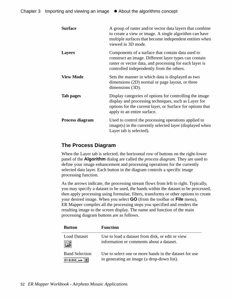
The Process Diagram
When the Layer tab is selected, the horizontal row of buttons on the right-lowpanel of the Algorithm dialog are called the process diagram. They are used to define your image enhancement and processing operations for the currently selected data layer. Each button in the diagram controls a specific image processing function.
As the arrows indicate, the processing stream flows from left to right. Typicallyou may specify a dataset to be used, the bands within the dataset to be procthen apply processing using formulae, filters, transforms or other options to cyour desired image. When you select GO (from the toolbar or File menu), ER Mapper compiles all the processing steps you specified and renders the resulting image to the screen display. The name and function of the main processing diagram buttons are as follows.
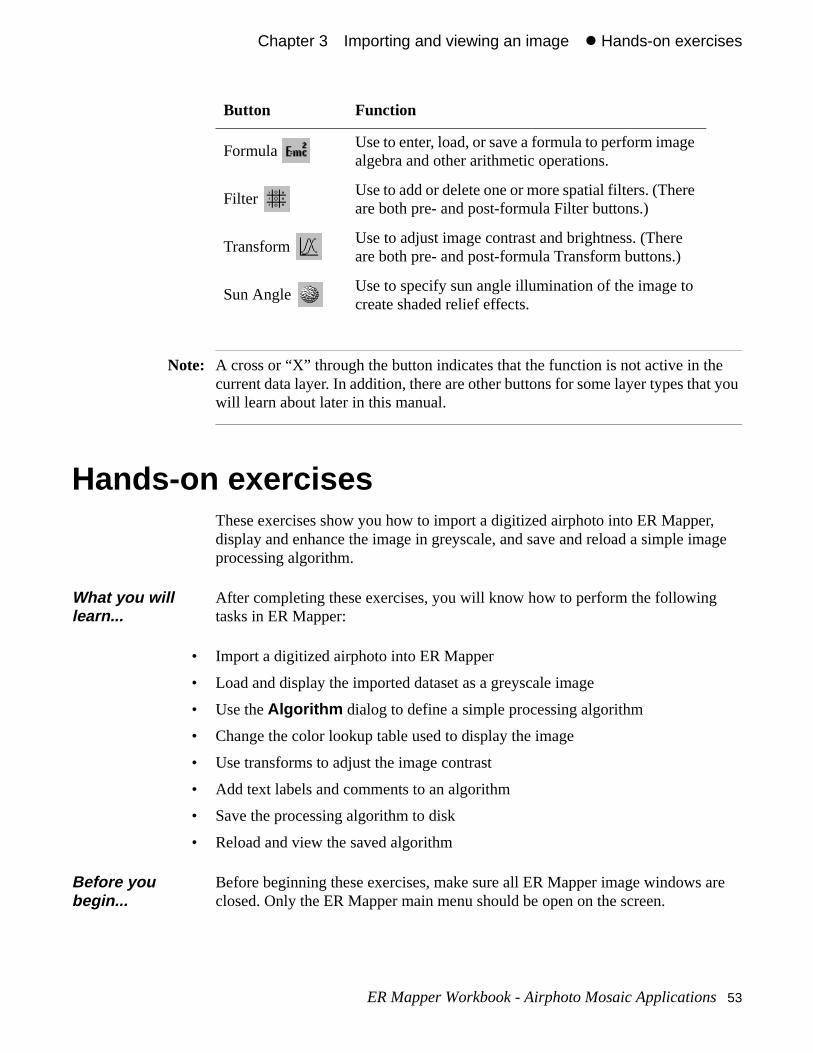
Button Function
Load Dataset Use to load a dataset from disk, or edit or view information or comments about a dataset.
Band Selection Use to select one or more bands in the dataset for use in generating an image (a drop-down list).
52 ER Mapper Workbook - Airphoto Mosaic Applications
Chapter 3#Importing and viewing an image#z Hands-on exercises
e t you
, age
are
Note: A cross or “X” through the button indicates that the function is not active in thcurrent data layer. In addition, there are other buttons for some layer types thawill learn about later in this manual.
Hands-on exercisesThese exercises show you how to import a digitized airphoto into ER Mapperdisplay and enhance the image in greyscale, and save and reload a simple improcessing algorithm.
• Import a digitized airphoto into ER Mapper
• Load and display the imported dataset as a greyscale image
• Use the Algorithm dialog to define a simple processing algorithm
• Change the color lookup table used to display the image
• Use transforms to adjust the image contrast
• Add text labels and comments to an algorithm
• Save the processing algorithm to disk
• Reload and view the saved algorithm
Formula Use to enter, load, or save a formula to perform image algebra and other arithmetic operations.
Filter Use to add or delete one or more spatial filters. (There are both pre- and post-formula Filter buttons.)
Transform Use to adjust image contrast and brightness. (There are both pre- and post-formula Transform buttons.)
Sun Angle Use to specify sun angle illumination of the image to create shaded relief effects.
What you will learn...
After completing these exercises, you will know how to perform the following tasks in ER Mapper:
Before you begin...
Before beginning these exercises, make sure all ER Mapper image windows closed. Only the ER Mapper main menu should be open on the screen.
Button Function
ER Mapper Workbook - Airphoto Mosaic Applications 53
Chapter 3#Importing and viewing an image#z 1: Opening an airphoto image file
or
r
1: Opening an airphoto image file
Note: The sample airphoto applications training datasets must be installed on your computer before you can complete this exercise. See Appendix A if needed fmore information.
About imputting dataYou can open any of the following image data formats directly into ER Mppaewithout having to import them as ER Mapper Raster Datasets:
• ER Mapper Algorithm (.alg)
• ER Mapper Raster Dataset (ers)
• ER Mapper Compressed Image (.ecw)
• Vector Map (.erv)
• Windows Bitmap (.bmp)
• ESRI BIL and GeoSPOT (.hdr)
• GeoTIFF/TIFF (.tif)
• JPEG (.jpg)
• USGS DOQQ (Grayscale)
• RESTEC/NASDA CEOS (.dat)
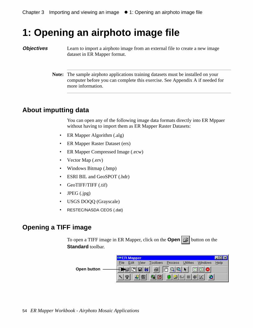
Opening a TIFF image
To open a TIFF image in ER Mapper, click on the Open button on the
Standard toolbar.
Objectives Learn to import a airphoto image from an external file to create a new image dataset in ER Mapper format.
Open button
54 ER Mapper Workbook - Airphoto Mosaic Applications
Chapter 3#Importing and viewing an image#z 1: Opening an airphoto image file
nts l
you
ort
t into ine
taset e
In the Open dialog box, select ‘GeoTIFF/TIFF(.tif)’ from the Files of Type list, and then select the TIFF image to be opened in ER Mapper.
You can add TIFF images to Algorithms and perform most image enhancemeon them. ER Mapper adds a header file with a .ers extension to hold statisticainformation about the image.
The Geocoding Wizard will only rectify ER Mapper Raster Dataset images. If want to rectify a TIFF image you must either save it as an ER Mapper RasterDataset or originally import it as an ER Mapper Raster Dataset.
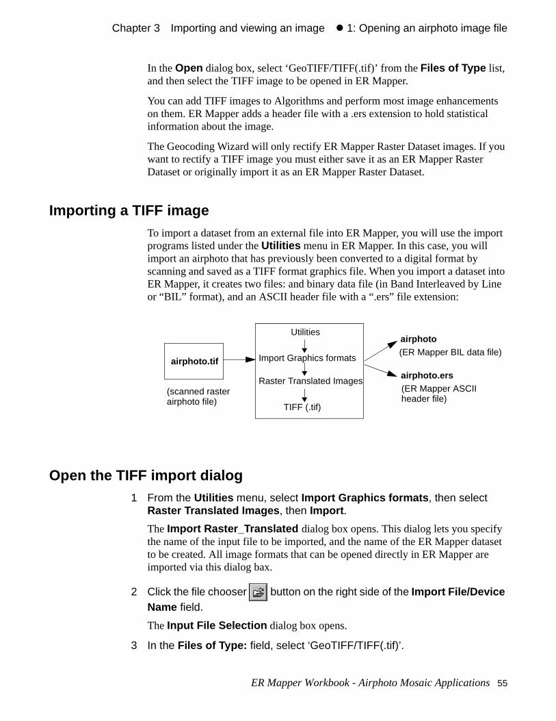
Importing a TIFF imageTo import a dataset from an external file into ER Mapper, you will use the impprograms listed under the Utilities menu in ER Mapper. In this case, you will import an airphoto that has previously been converted to a digital format by scanning and saved as a TIFF format graphics file. When you import a dataseER Mapper, it creates two files: and binary data file (in Band Interleaved by Lor “BIL” format), and an ASCII header file with a “.ers” file extension:
Open the TIFF import dialog1 From the Utilities menu, select Import Graphics formats , then select
Raster Translated Images , then Import .
The Import Raster_Translated dialog box opens. This dialog lets you specifythe name of the input file to be imported, and the name of the ER Mapper dato be created. All image formats that can be opened directly in ER Mapper arimported via this dialog bax.
2 Click the file chooser button on the right side of the Import File/Device Name field.
The Input File Selection dialog box opens.
3 In the Files of Type: field, select ‘GeoTIFF/TIFF(.tif)’.
(scanned rasterairphoto file)
airphoto.tif
Utilities
Import Graphics formats
TIFF (.tif)
airphoto.ers(ER Mapper ASCII
airphoto(ER Mapper BIL data file)
header file)
Raster Translated Images
ER Mapper Workbook - Airphoto Mosaic Applications 55
Chapter 3#Importing and viewing an image#z 2: Displaying an image in greyscale
rmat.
:
white he
or
4 From the Directories menu (on the Input File dialog), select the path ending with \examples .
5 Double-click on the directory named ‘Shared_Data’ and then the directory named ‘airphoto_training.’
6 Double-click on the image file named ‘photo_86.tif’ to load it.
7 Click the file chooser button next to the Output Dataset Name field.
The Output Dataset Selection dialog box opens.
8 From the Directories menu (on the Output Dataset dialog), select the path ending with \examples .
9 Double-click on the directory named ‘airphoto_training.’
10 In the Save As: field, enter the text raw_photo_86 then click OK.
11 Click OK on the Import TIFF dialog.
ER Mapper reads the TIFF file and begins creating a dataset in ER Mapper fo
12 When the import finishes, click OK on the confirmation dialog, then click Cancel on the Import Raster_Translated dialog.
In this case, ER Mapper translated the TIFF image data and created two files
• ‘raw_photo_86’ (the binary data file)
• ‘raw_photo_86.ers’ (the ASCII header file)
2: Displaying an image in greyscale
Note: The airphoto you imported is a color photograph. You will initially learn to viewand adjust the photo as a greyscale image, which is appropriate for black andaerial photographs. Later you will learn to view it as an RGB color image (in tfollowing chapter).
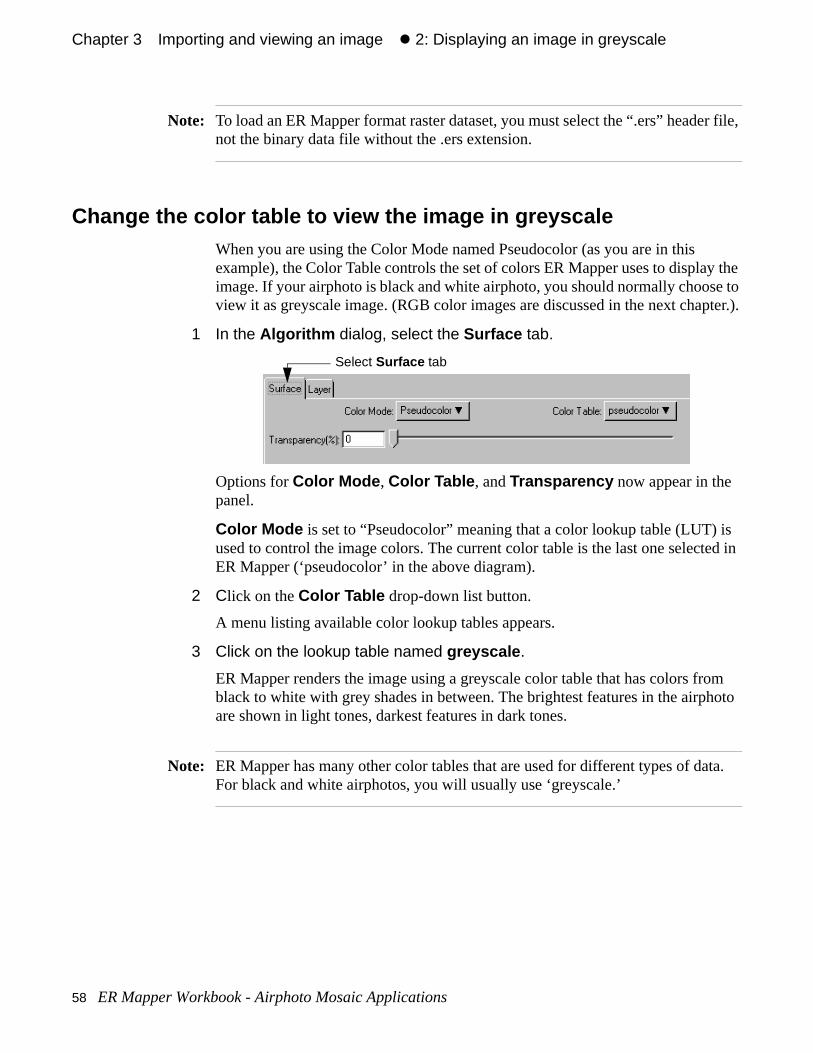
Open an image window and the Algorithm dialog1 From the View menu, select Algorithm... .
Objectives Learn to open an image window and the Algorithm dialog, load an image, and display the image in greyscale. You will also learn to change the contrast (colmapping) of the image.
56 ER Mapper Workbook - Airphoto Mosaic Applications
Chapter 3#Importing and viewing an image#z 2: Displaying an image in greyscale
the
for
as y.
ple
not
r. Note
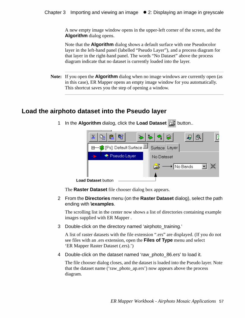
A new empty image window opens in the upper-left corner of the screen, andAlgorithm dialog opens.
Note that the Algorithm dialog shows a default surface with one Pseudocolor layer in the left-hand panel (labelled “Pseudo Layer”), and a process diagramthat layer in the right-hand panel. The words “No Dataset” above the processdiagram indicate that no dataset is currently loaded into the layer.
Note: If you open the Algorithm dialog when no image windows are currently open (in this case), ER Mapper opens an empty image window for you automaticallThis shortcut saves you the step of opening a window.
Load the airphoto dataset into the Pseudo layer
1 In the Algorithm dialog, click the Load Dataset button..
The Raster Dataset file chooser dialog box appears.
2 From the Directories menu (on the Raster Dataset dialog), select the path ending with \examples .
The scrolling list in the center now shows a list of directories containing examimages supplied with ER Mapper .
3 Double-click on the directory named ‘airphoto_training.’
A list of raster datasets with the file extension “.ers” are displayed. (If you do see files with an .ers extension, open the Files of Type menu and select ‘ER Mapper Raster Dataset (.ers).’)
4 Double-click on the dataset named ‘raw_photo_86.ers’ to load it.
The file chooser dialog closes, and the dataset is loaded into the Pseudo layethat the dataset name (‘raw_photo_ap.ers’) now appears above the process diagram.
Load Dataset button
ER Mapper Workbook - Airphoto Mosaic Applications 57
Chapter 3#Importing and viewing an image#z 2: Displaying an image in greyscale
r file,
y the e to pter.).
is ted in
om hoto
ta.
Note: To load an ER Mapper format raster dataset, you must select the “.ers” headenot the binary data file without the .ers extension.
Change the color table to view the image in greyscaleWhen you are using the Color Mode named Pseudocolor (as you are in this example), the Color Table controls the set of colors ER Mapper uses to displaimage. If your airphoto is black and white airphoto, you should normally choosview it as greyscale image. (RGB color images are discussed in the next cha
1 In the Algorithm dialog, select the Surface tab.
Options for Color Mode , Color Table , and Transparency now appear in the panel.
Color Mode is set to “Pseudocolor” meaning that a color lookup table (LUT) used to control the image colors. The current color table is the last one selecER Mapper (‘pseudocolor’ in the above diagram).
2 Click on the Color Table drop-down list button.
A menu listing available color lookup tables appears.
3 Click on the lookup table named greyscale .
ER Mapper renders the image using a greyscale color table that has colors frblack to white with grey shades in between. The brightest features in the airpare shown in light tones, darkest features in dark tones.
Note: ER Mapper has many other color tables that are used for different types of daFor black and white airphotos, you will usually use ‘greyscale.’
Select Surface tab
58 ER Mapper Workbook - Airphoto Mosaic Applications
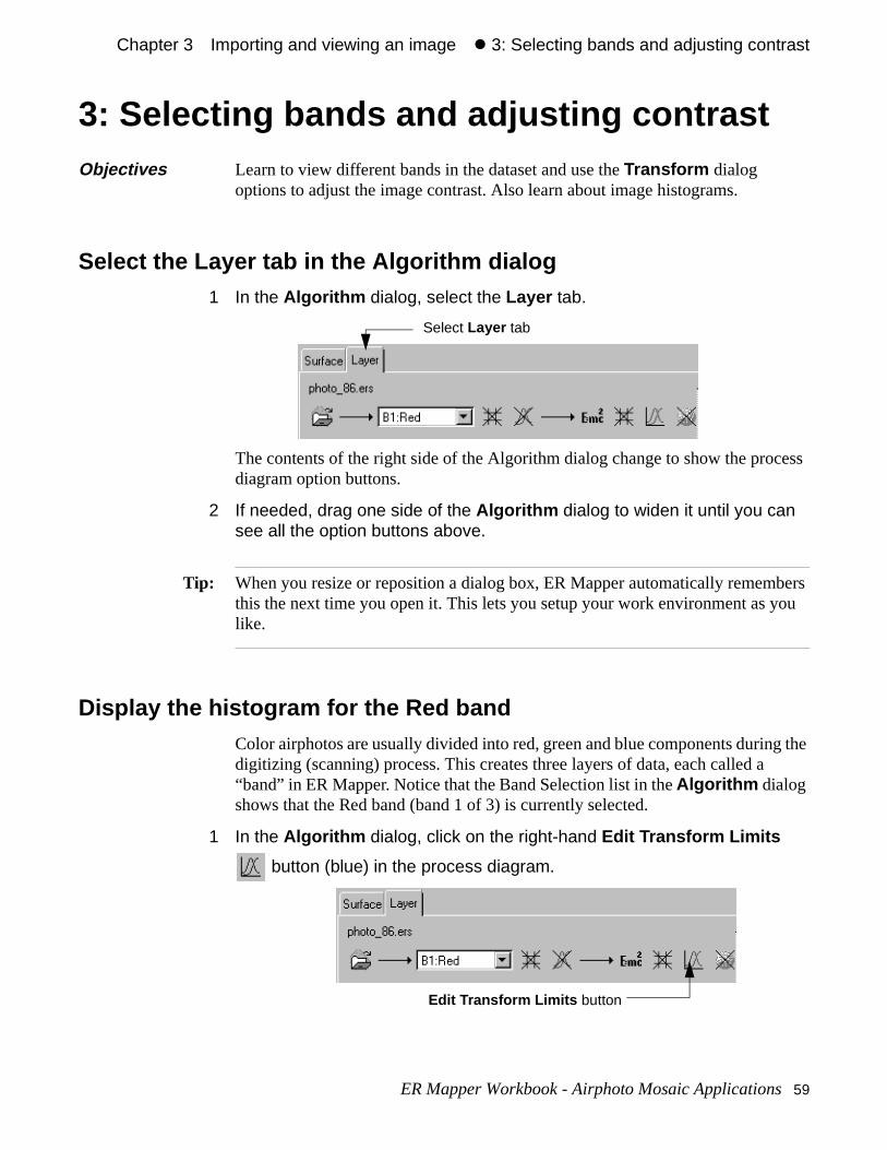
Chapter 3#Importing and viewing an image#z 3: Selecting bands and adjusting contrast
cess
bers ou
g the
3: Selecting bands and adjusting contrast
Select the Layer tab in the Algorithm dialog1 In the Algorithm dialog, select the Layer tab.
The contents of the right side of the Algorithm dialog change to show the prodiagram option buttons.
2 If needed, drag one side of the Algorithm dialog to widen it until you can see all the option buttons above.
Tip: When you resize or reposition a dialog box, ER Mapper automatically rememthis the next time you open it. This lets you setup your work environment as ylike.
Display the histogram for the Red bandColor airphotos are usually divided into red, green and blue components durindigitizing (scanning) process. This creates three layers of data, each called a“band” in ER Mapper. Notice that the Band Selection list in the Algorithm dialog shows that the Red band (band 1 of 3) is currently selected.
1 In the Algorithm dialog, click on the right-hand Edit Transform Limits
button (blue) in the process diagram.
Objectives Learn to view different bands in the dataset and use the Transform dialog options to adjust the image contrast. Also learn about image histograms.
Select Layer tab
Edit Transform Limits button
ER Mapper Workbook - Airphoto Mosaic Applications 59
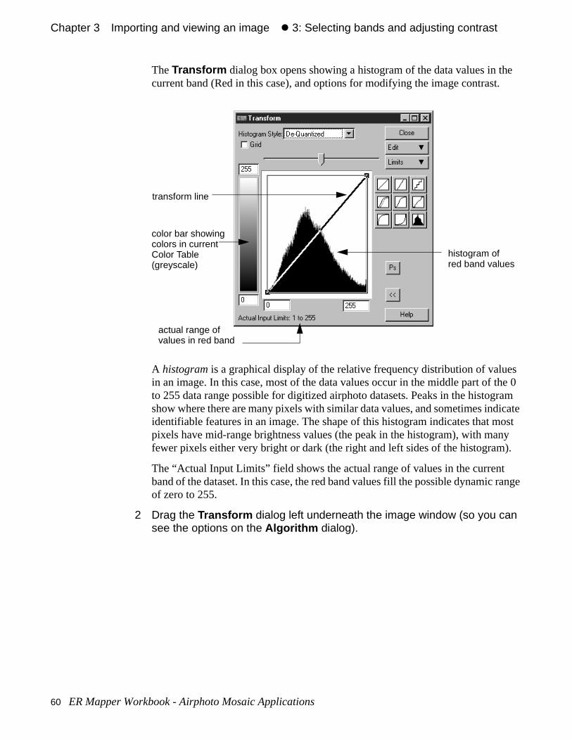
Chapter 3#Importing and viewing an image#z 3: Selecting bands and adjusting contrast
he .
es he 0 ram icate ost ny ).
range
The Transform dialog box opens showing a histogram of the data values in tcurrent band (Red in this case), and options for modifying the image contrast
A histogram is a graphical display of the relative frequency distribution of valuin an image. In this case, most of the data values occur in the middle part of tto 255 data range possible for digitized airphoto datasets. Peaks in the histogshow where there are many pixels with similar data values, and sometimes indidentifiable features in an image. The shape of this histogram indicates that mpixels have mid-range brightness values (the peak in the histogram), with mafewer pixels either very bright or dark (the right and left sides of the histogram
The “Actual Input Limits” field shows the actual range of values in the currentband of the dataset. In this case, the red band values fill the possible dynamicof zero to 255.
2 Drag the Transform dialog left underneath the image window (so you can see the options on the Algorithm dialog).
histogram ofred band values
transform line
actual range ofvalues in red band
color bar showingcolors in currentColor Table(greyscale)
60 ER Mapper Workbook - Airphoto Mosaic Applications
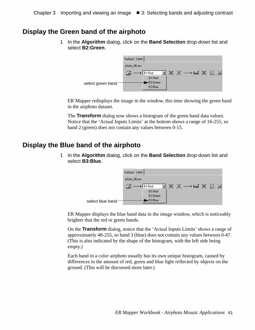
Chapter 3#Importing and viewing an image#z 3: Selecting bands and adjusting contrast
and
. so
ably
of 0-47.
y the
Display the Green band of the airphoto1 In the Algorithm dialog, click on the Band Selection drop-down list and
select B2:Green .
ER Mapper redisplays the image in the window, this time showing the green bin the airphoto dataset.
The Transform dialog now shows a histogram of the green band data valuesNotice that the ‘Actual Inputs Limits’ at the bottom shows a range of 16-255, band 2 (green) does not contain any values between 0-15.
Display the Blue band of the airphoto1 In the Algorithm dialog, click on the Band Selection drop-down list and
select B3:Blue .
ER Mapper displays the blue band data in the image window, which is noticebrighter that the red or green bands.
On the Transform dialog, notice that the ‘Actual Inputs Limits’ shows a range approximately 48-255, so band 3 (blue) does not contain any values between(This is also indicated by the shape of the histogram, with the left side being empty.)
Each band in a color airphoto usually has its own unique histogram, caused bdifferences in the amount of red, green and blue light reflected by objects on ground. (This will be discussed more later.)
select green band
select blue band
ER Mapper Workbook - Airphoto Mosaic Applications 61
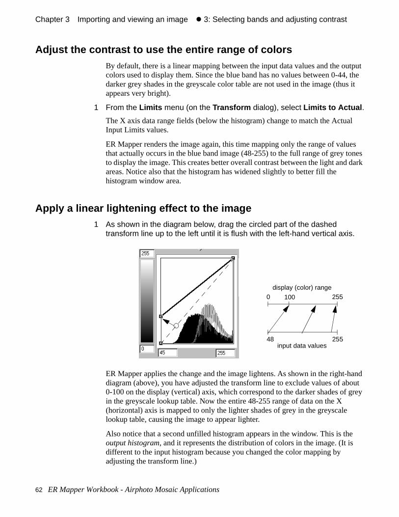
Chapter 3#Importing and viewing an image#z 3: Selecting bands and adjusting contrast
utput 4, the s it
al
es ones dark
hand bout grey
e
Adjust the contrast to use the entire range of colorsBy default, there is a linear mapping between the input data values and the ocolors used to display them. Since the blue band has no values between 0-4darker grey shades in the greyscale color table are not used in the image (thuappears very bright).
1 From the Limits menu (on the Transform dialog), select Limits to Actual .
The X axis data range fields (below the histogram) change to match the ActuInput Limits values.
ER Mapper renders the image again, this time mapping only the range of valuthat actually occurs in the blue band image (48-255) to the full range of grey tto display the image. This creates better overall contrast between the light andareas. Notice also that the histogram has widened slightly to better fill the histogram window area.
Apply a linear lightening effect to the image1 As shown in the diagram below, drag the circled part of the dashed
transform line up to the left until it is flush with the left-hand vertical axis.
ER Mapper applies the change and the image lightens. As shown in the right-diagram (above), you have adjusted the transform line to exclude values of a0-100 on the display (vertical) axis, which correspond to the darker shades ofin the greyscale lookup table. Now the entire 48-255 range of data on the X (horizontal) axis is mapped to only the lighter shades of grey in the greyscalelookup table, causing the image to appear lighter.
Also notice that a second unfilled histogram appears in the window. This is thoutput histogram, and it represents the distribution of colors in the image. (It isdifferent to the input histogram because you changed the color mapping by adjusting the transform line.)
48 255input data values
0 255
display (color) range
100
62 ER Mapper Workbook - Airphoto Mosaic Applications
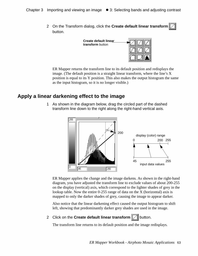
Chapter 3#Importing and viewing an image#z 3: Selecting bands and adjusting contrast
ame
-hand -255 the
er.
ift
2 On the Transform dialog, click the Create default linear transform button.
ER Mapper returns the transform line to its default position and redisplays theimage. (The default position is a straight linear transform, where the line’s X position is equal to its Y position. This also makes the output histogram the sas the input histogram, so it is no longer visible.)
Apply a linear darkening effect to the image1 As shown in the diagram below, drag the circled part of the dashed
transform line down to the right along the right-hand vertical axis.
ER Mapper applies the change and the image darkens. As shown in the rightdiagram, you have adjusted the transform line to exclude values of about 200on the display (vertical) axis, which correspond to the lighter shades of grey inlookup table. Now the entire 0-255 range of data on the X (horizontal) axis is mapped to only the darker shades of grey, causing the image to appear dark
Also notice that the linear darkening effect caused the output histogram to shleft, showing that predominantly darker grey shades are used in the image.
2 Click on the Create default linear transform button.
The transform line returns to its default position and the image redisplays.
Create default lineartransform button
45 255input data values
0 255
display (color) range
200
200
ER Mapper Workbook - Airphoto Mosaic Applications 63
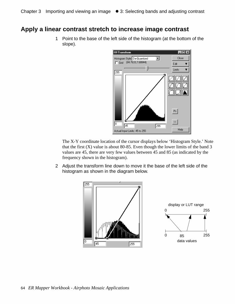
Chapter 3#Importing and viewing an image#z 3: Selecting bands and adjusting contrast
ote d 3 the
Apply a linear contrast stretch to increase image contrast1 Point to the base of the left side of the histogram (at the bottom of the
slope).
The X-Y coordinate location of the cursor displays below ‘Histogram Style.’ Nthat the first (X) value is about 80-85. Even though the lower limits of the banvalues are 45, there are very few values between 45 and 85 (as indicated byfrequency shown in the histogram).
2 Adjust the transform line down to move it the base of the left side of the histogram as shown in the diagram below.
0 255
data values
0 255
display or LUT range
85
64 ER Mapper Workbook - Airphoto Mosaic Applications
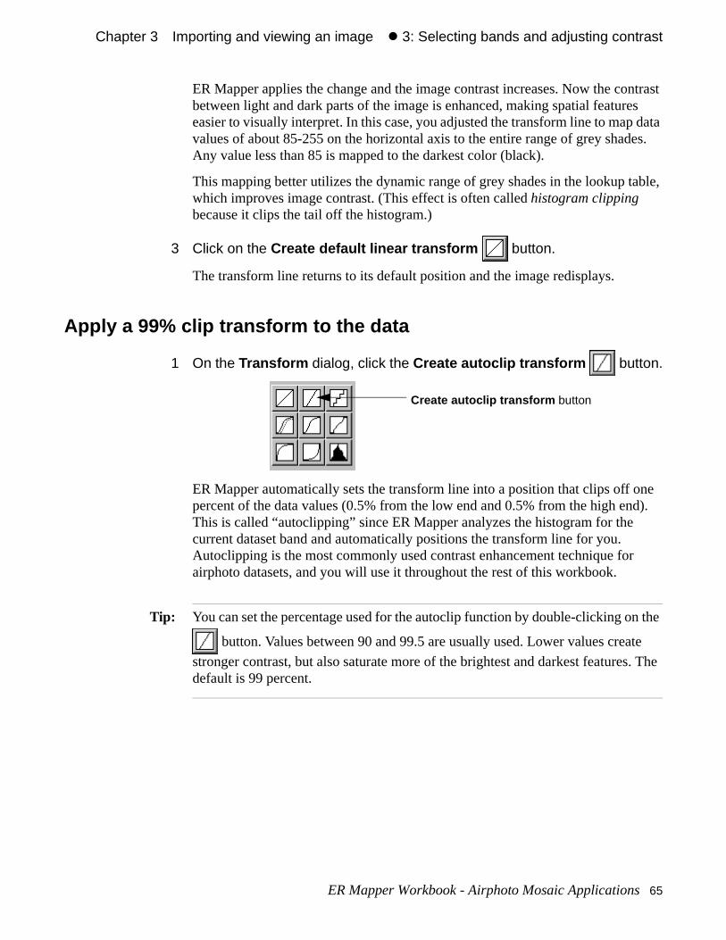
Chapter 3#Importing and viewing an image#z 3: Selecting bands and adjusting contrast
ntrast es data es.
able,
ne d).
n the
te
s. The
ER Mapper applies the change and the image contrast increases. Now the cobetween light and dark parts of the image is enhanced, making spatial featureasier to visually interpret. In this case, you adjusted the transform line to mapvalues of about 85-255 on the horizontal axis to the entire range of grey shadAny value less than 85 is mapped to the darkest color (black).
This mapping better utilizes the dynamic range of grey shades in the lookup twhich improves image contrast. (This effect is often called histogram clipping because it clips the tail off the histogram.)
3 Click on the Create default linear transform button.
The transform line returns to its default position and the image redisplays.
Apply a 99% clip transform to the data
1 On the Transform dialog, click the Create autoclip transform button.
ER Mapper automatically sets the transform line into a position that clips off opercent of the data values (0.5% from the low end and 0.5% from the high enThis is called “autoclipping” since ER Mapper analyzes the histogram for the current dataset band and automatically positions the transform line for you. Autoclipping is the most commonly used contrast enhancement technique forairphoto datasets, and you will use it throughout the rest of this workbook.
Tip: You can set the percentage used for the autoclip function by double-clicking o
button. Values between 90 and 99.5 are usually used. Lower values crea
stronger contrast, but also saturate more of the brightest and darkest featuredefault is 99 percent.
Create autoclip transform button
ER Mapper Workbook - Airphoto Mosaic Applications 65
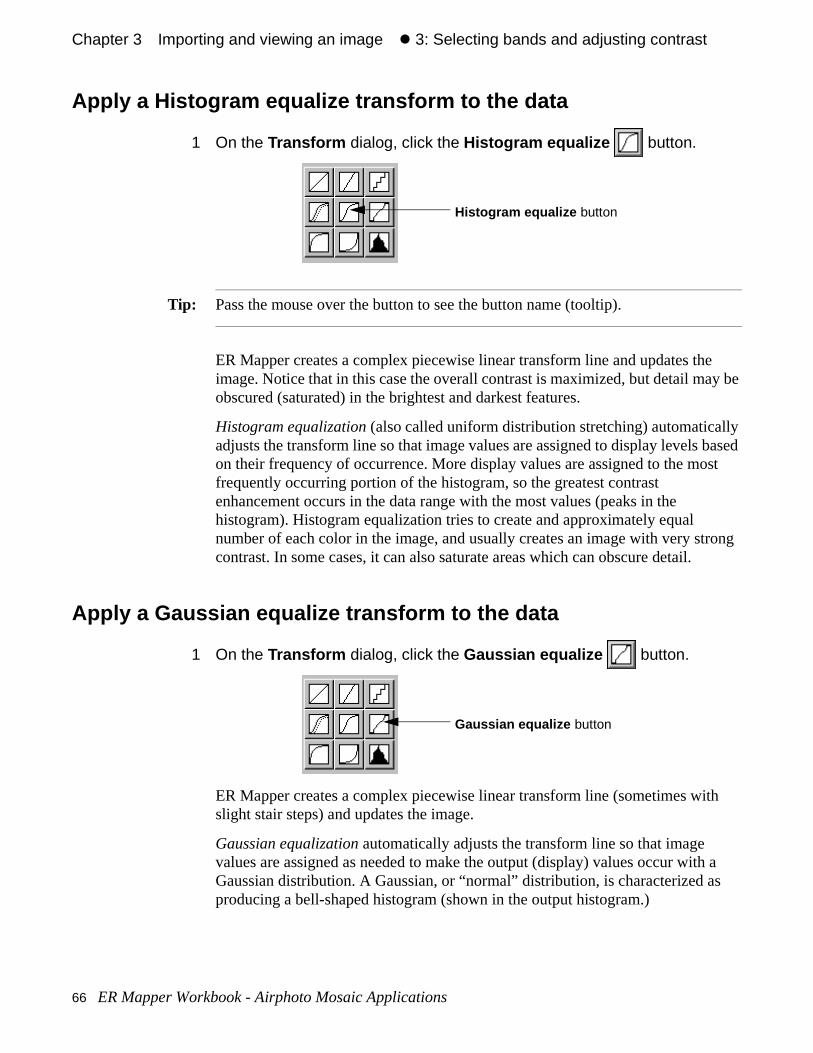
Chapter 3#Importing and viewing an image#z 3: Selecting bands and adjusting contrast
e y be
ly based st
rong
th
h a s
Apply a Histogram equalize transform to the data
1 On the Transform dialog, click the Histogram equalize button.
Tip: Pass the mouse over the button to see the button name (tooltip).
ER Mapper creates a complex piecewise linear transform line and updates thimage. Notice that in this case the overall contrast is maximized, but detail maobscured (saturated) in the brightest and darkest features.
Histogram equalization (also called uniform distribution stretching) automaticaladjusts the transform line so that image values are assigned to display levelson their frequency of occurrence. More display values are assigned to the mofrequently occurring portion of the histogram, so the greatest contrast enhancement occurs in the data range with the most values (peaks in the histogram). Histogram equalization tries to create and approximately equal number of each color in the image, and usually creates an image with very stcontrast. In some cases, it can also saturate areas which can obscure detail.
Apply a Gaussian equalize transform to the data
1 On the Transform dialog, click the Gaussian equalize button.
ER Mapper creates a complex piecewise linear transform line (sometimes wislight stair steps) and updates the image.
Gaussian equalization automatically adjusts the transform line so that image values are assigned as needed to make the output (display) values occur witGaussian distribution. A Gaussian, or “normal” distribution, is characterized aproducing a bell-shaped histogram (shown in the output histogram.)
Histogram equalize button
Gaussian equalize button
66 ER Mapper Workbook - Airphoto Mosaic Applications
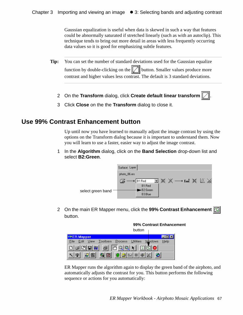
Chapter 3#Importing and viewing an image#z 3: Selecting bands and adjusting contrast
res This g
e
.
the Now
, and
Gaussian equalization is useful when data is skewed in such a way that featucould be abnormally saturated if stretched linearly (such as with an autoclip). technique tends to bring out more detail in areas with less frequently occurrindata values so it is good for emphasizing subtle features.
Tip: You can set the number of standard deviations used for the Gaussian equaliz
function by double-clicking on the button. Smaller values produce more
contrast and higher values less contrast. The default is 3 standard deviations
2 On the Transform dialog, click Create default linear transform .
3 Click Close on the the Transform dialog to close it.
Use 99% Contrast Enhancement buttonUp until now you have learned to manually adjust the image contrast by usingoptions on the Transform dialog because it is important to understand them. you will learn to use a faster, easier way to adjust the image contrast.
1 In the Algorithm dialog, click on the Band Selection drop-down list and select B2:Green .
2 On the main ER Mapper menu, click the 99% Contrast Enhancement
button.
ER Mapper runs the algorithm again to display the green band of the airphotoautomatically adjusts the contrast for you. This button performs the following sequence or actions for you automatically:
select green band
99% Contrast Enhancementbutton
ER Mapper Workbook - Airphoto Mosaic Applications 67
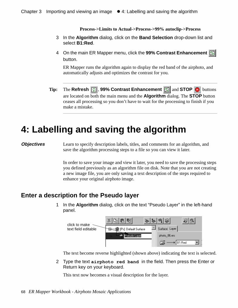
Chapter 3#Importing and viewing an image#z 4: Labelling and saving the algorithm
nd
you
steps ting
to
cted.
Process->Limits to Actual->Process->99% autoclip->Process
3 In the Algorithm dialog, click on the Band Selection drop-down list and select B1:Red .
4 On the main ER Mapper menu, click the 99% Contrast Enhancement button.
ER Mapper runs the algorithm again to display the red band of the airphoto, aautomatically adjusts and optimizes the contrast for you.
Tip: The Refresh , 99% Contrast Enhancement and STOP buttons
are located on both the main menu and the Algorithm dialog. The STOP button ceases all processing so you don’t have to wait for the processing to finish if make a mistake.
4: Labelling and saving the algorithm
In order to save your image and view it later, you need to save the processingyou defined previously as an algorithm file on disk. Note that you are not creaa new image file, you are only saving a text description of the steps required enhance your original airphoto image.
Enter a description for the Pseudo layer1 In the Algorithm dialog, click on the text “Pseudo Layer” in the left-hand
panel.
The text become reverse highlighted (shown above) indicating the text is sele
2 Type the text airphoto red band in the field. Then press the Enter or Return key on your keyboard.
This text now becomes a visual description for the layer.
Objectives Learn to specify description labels, titles, and comments for an algorithm, andsave the algorithm processing steps to a file so you can view it later.
click to maketext field editable
68 ER Mapper Workbook - Airphoto Mosaic Applications
Chapter 3#Importing and viewing an image#z 4: Labelling and saving the algorithm
t it,
.)
k.
rea
Note: If a layer is not already selected (highlighted), click once on the layer to selecthen click a second time on the text label to make it editable.
Enter a description for the entire algorithm1 In the Algorithm dialog, select the text in the Description text field (it
currently reads ‘No Description’).
(To select the text, either drag through it, or triple-click to select the entire line
2 Type the following text, then press Enter or Return on your keyboard:
San Diego airphoto 86 in greyscale
This text now becomes a brief description for the entire algorithm.
Save the processing steps to an algorithm file on disk1 From the File menu (on the main menu), select Save As... .
The Save Algorithm file chooser dialog opens.
2 From the Directories menu, select the path ending with the text \examples . (The portion of the path name preceding it is specific to your site.)
3 Double-click on the directory named ‘airphoto_training’ to open it.
4 In the Save As: text field, click to place the cursor, then type the following name for the algorithm file:
Airphoto_86_greyscale
5 Click the Apply button to save the algorithm and leave the dialog open.
Your pseudocolor greyscale algorithm is now saved to an algorithm file on dis
Add comments to the algorithm1 On the Save Algorithm dialog, click the Comments... button.
A dialog box appears titled with the algorithm path and file name, and a text ato type comments about your algorithm. The cursor is already active.
2 In the comments dialog, type the following information to describe your algorithm:
This algorithm displays the red band of Tustin airphoto 86
as a greyscale algorithm. A 99% autoclip transform is used
ER Mapper Workbook - Airphoto Mosaic Applications 69
Chapter 3#Importing and viewing an image#z 5: Reloading and viewing the algorithm
ou
the me
to increase image contrast.
3 Click OK on the comments dialog to save your comments.
4 Click Cancel on the Save Algorithm dialog close it.
5: Reloading and viewing the algorithm
Open a second image window1 On the Standard toolbar (on the main menu), click the New Image
Window button.
ER Mapper opens a new image window (this is a shortcut for selecting New from the File menu). Drag the new window to the lower left part of the screen (so ycan see all or most of the other image window).
Open the greyscale algorithm you created earlier
1 On the main menu, click on the Open button.
The Open file chooser dialog appears. (This is a shortcut for selecting Open... from the File menu.)
2 From the Directories menu, select the path ending with the text \examples .
3 From the Files of Type: list, select ‘ER Mapper Algorithm (.alg)’.
4 Double-click on the directory named ‘airphoto_training’ to open it.
Your ‘Airphoto_86_greyscale’ algorithm name should appear in the list.
5 Click once on your algorithm name to highlight it (do not double-click).
6 Click the Apply button to load and process the algorithm without closing the Open dialog box.
ER Mapper runs the algorithm and displays the enhanced airphoto dataset inimage window. It looks identical to the other image since they both use the saalgorithm and dataset.
Objectives Learn to reload and display the algorithm you just created.
70 ER Mapper Workbook - Airphoto Mosaic Applications

Chapter 3#Importing and viewing an image#z 5: Reloading and viewing the algorithm
ithm,
s
View the algorithm comments1 On the Open dialog, click the Comments... button.
The dialog box opens showing the comments you entered for your algorithm.These comments can be very helpful to others who use or display your algorand they are a good way to document the procedures you used to create it.
2 Click Cancel on the comments dialog box to close it.
Close both image windows and the Algorithm dialog1 Close the lower image window:
• For Windows, click the Close button in the upper-right window corner.
2 Close the other image window by repeating Step 1.
3 On the Algorithm dialog, click the Close button.
Only the ER Mapper main menu is now open on the screen.
• Import a digitized airphoto into ER Mapper
• Load and display the imported dataset as a greyscale image
• Use the Algorithm dialog to define a simple processing algorithm
• Change the color lookup table used to display the image
• Use transforms to adjust the image contrast
• Add text labels and comments to an algorithm
• Save the processing algorithm to disk
• Reload and view the saved algorithm
What you learned...
After completing these exercises, you know how to perform the following taskin ER Mapper:
ER Mapper Workbook - Airphoto Mosaic Applications 71

Chapter 3#Importing and viewing an image#z 5: Reloading and viewing the algorithm
72 ER Mapper Workbook - Airphoto Mosaic Applications
hms.
of
at ly w ed m.) any ite is r in
4
Viewing an imagein RGB
This chapter shows you how to display an airphoto dataset as an RGB color composite image. You also learn how to manipulate layers on the Algorithm dialog, and how to use wizards for viewing datasets and creating RGB algorit
About RGB color imagesIn the RGB color system, each color is created by mixing different proportionsthe three additive primary colors–red, green and blue. Computers create color by lighting up an array of tiny red, green and blue phosphors on the screen.
For example, to create a green pixel on the screen, the green phosphor for thpixel is lit up to its full intensity, and the red and blue phosphors are essentialturned off. (This might be a park or golf course for example.) To create a yellopixel, the red and green phosphors are set to full intensity and the blue is turnoff. (Red and green together combine to create yellow in the RGB color systeBy combining various proportions of the three additive primary colors, nearly color can be created. When all three phosphors are lit to their full intensity whcreated, when all are turned off black results. When red, green and blue occuequal proportions, grey is produced.
ER Mapper Workbook - Airphoto Mosaic Applications 73
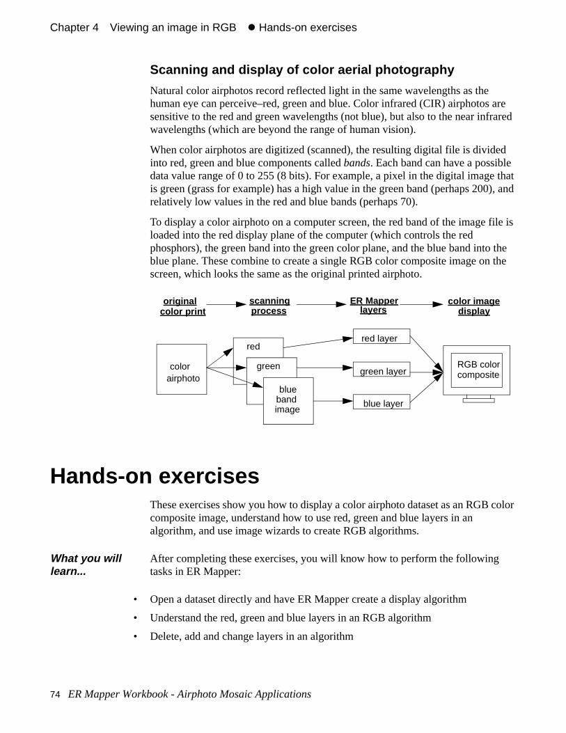
Chapter 4#Viewing an image in RGB#z Hands-on exercises
are rared
d
that ), and
file is
the the
color
Scanning and display of color aerial photography
Natural color airphotos record reflected light in the same wavelengths as the human eye can perceive–red, green and blue. Color infrared (CIR) airphotossensitive to the red and green wavelengths (not blue), but also to the near infwavelengths (which are beyond the range of human vision).
When color airphotos are digitized (scanned), the resulting digital file is divideinto red, green and blue components called bands. Each band can have a possibledata value range of 0 to 255 (8 bits). For example, a pixel in the digital imageis green (grass for example) has a high value in the green band (perhaps 200relatively low values in the red and blue bands (perhaps 70).
To display a color airphoto on a computer screen, the red band of the image loaded into the red display plane of the computer (which controls the red phosphors), the green band into the green color plane, and the blue band intoblue plane. These combine to create a single RGB color composite image onscreen, which looks the same as the original printed airphoto.
Hands-on exercisesThese exercises show you how to display a color airphoto dataset as an RGBcomposite image, understand how to use red, green and blue layers in an algorithm, and use image wizards to create RGB algorithms.
• Open a dataset directly and have ER Mapper create a display algorithm
• Understand the red, green and blue layers in an RGB algorithm
• Delete, add and change layers in an algorithm
What you will learn...
After completing these exercises, you will know how to perform the following tasks in ER Mapper:
colorairphoto
original scanningprocess
ER Mapperlayers
color imagedisplay
redred layer
green layer
blue layer
color print
RGB colorcomposite
green
bluebandimage
74 ER Mapper Workbook - Airphoto Mosaic Applications
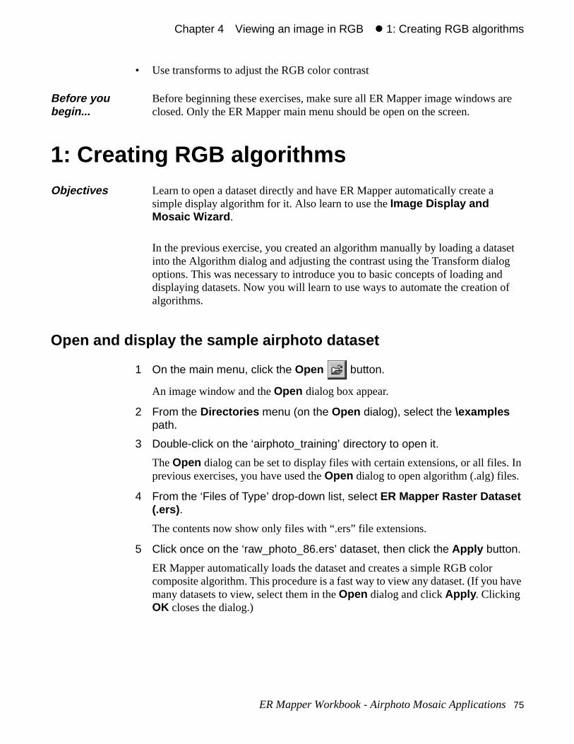
Chapter 4#Viewing an image in RGB#z 1: Creating RGB algorithms
set g d of
. In
have
are
• Use transforms to adjust the RGB color contrast
1: Creating RGB algorithms
In the previous exercise, you created an algorithm manually by loading a datainto the Algorithm dialog and adjusting the contrast using the Transform dialooptions. This was necessary to introduce you to basic concepts of loading andisplaying datasets. Now you will learn to use ways to automate the creation algorithms.
Open and display the sample airphoto dataset
1 On the main menu, click the Open button.
An image window and the Open dialog box appear.
2 From the Directories menu (on the Open dialog), select the \examples path.
3 Double-click on the ‘airphoto_training’ directory to open it.
The Open dialog can be set to display files with certain extensions, or all filesprevious exercises, you have used the Open dialog to open algorithm (.alg) files.
4 From the ‘Files of Type’ drop-down list, select ER Mapper Raster Dataset (.ers) .
The contents now show only files with “.ers” file extensions.
5 Click once on the ‘raw_photo_86.ers’ dataset, then click the Apply button.
ER Mapper automatically loads the dataset and creates a simple RGB color composite algorithm. This procedure is a fast way to view any dataset. (If you many datasets to view, select them in the Open dialog and click Apply . Clicking OK closes the dialog.)
Before you begin...
Before beginning these exercises, make sure all ER Mapper image windows closed. Only the ER Mapper main menu should be open on the screen.
Objectives Learn to open a dataset directly and have ER Mapper automatically create a simple display algorithm for it. Also learn to use the Image Display and Mosaic Wizard .
ER Mapper Workbook - Airphoto Mosaic Applications 75
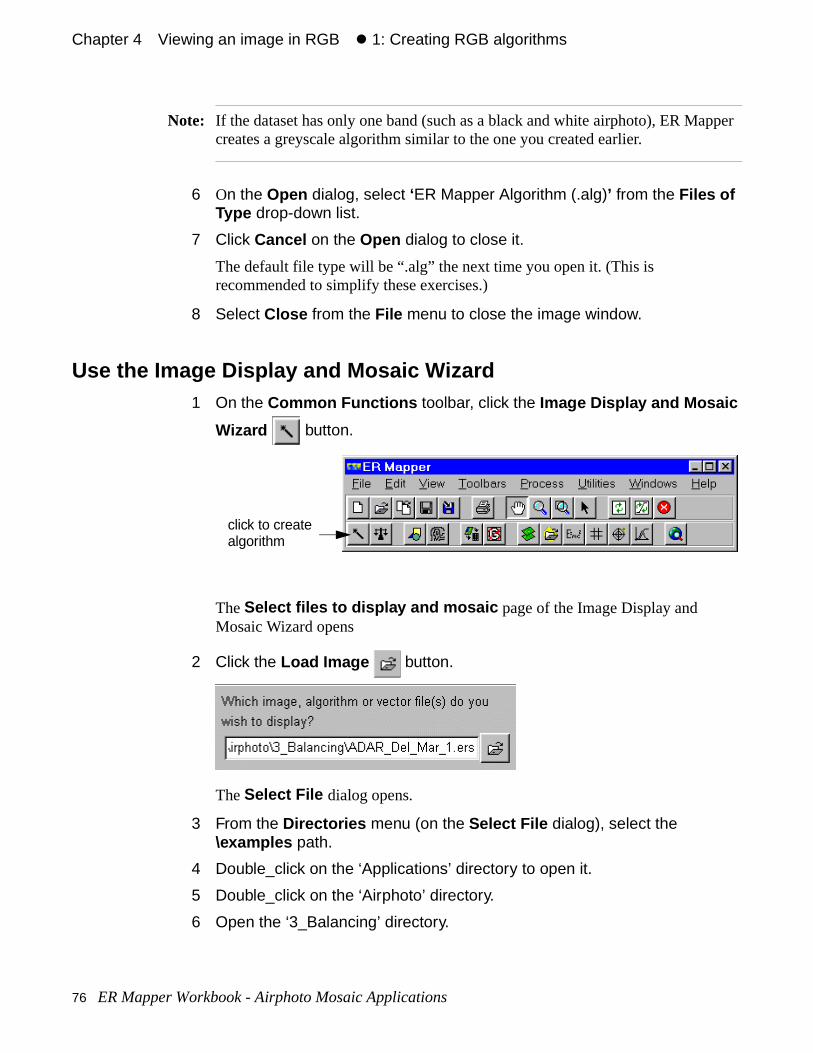
Chapter 4#Viewing an image in RGB#z 1: Creating RGB algorithms
pper
Note: If the dataset has only one band (such as a black and white airphoto), ER Macreates a greyscale algorithm similar to the one you created earlier.6 On the Open dialog, select ‘ER Mapper Algorithm (.alg)’ from the Files of Type drop-down list.
7 Click Cancel on the Open dialog to close it.
The default file type will be “.alg” the next time you open it. (This is recommended to simplify these exercises.)
8 Select Close from the File menu to close the image window.
Use the Image Display and Mosaic Wizard1 On the Common Functions toolbar, click the Image Display and Mosaic
Wizard button.
The Select files to display and mosaic page of the Image Display and Mosaic Wizard opens
2 Click the Load Image button.
The Select File dialog opens.
3 From the Directories menu (on the Select File dialog), select the \examples path.
4 Double_click on the ‘Applications’ directory to open it.
5 Double_click on the ‘Airphoto’ directory.
6 Open the ‘3_Balancing’ directory.
click to createalgorithm
76 ER Mapper Workbook - Airphoto Mosaic Applications
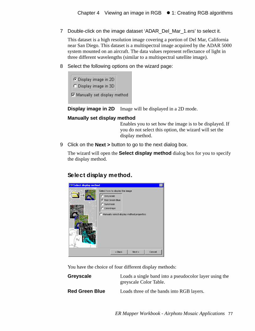
Chapter 4#Viewing an image in RGB#z 1: Creating RGB algorithms
ia 5000 in
If
e
7 Double-click on the image dataset ‘ADAR_Del_Mar_1.ers’ to select it.
This dataset is a high resolution image covering a portion of Del Mar, Californnear San Diego. This dataset is a multispectral image acquired by the ADAR system mounted on an aircraft. The data values represent reflectance of lightthree different wavelengths (similar to a multispectral satellite image).
8 Select the following options on the wizard page:
Display image in 2D Image will be displayed in a 2D mode.
Manually set display methodEnables you to set how the image is to be displayed.you do not select this option, the wizard will set the display method.
9 Click on the Next > button to go to the next dialog box.
The wizard will open the Select display method dialog box for you to specify the display method.
Select display method.
You have the choice of four different display methods:
Greyscale Loads a single band into a pseudocolor layer using thgreyscale Color Table.
Red Green Blue Loads three of the bands into RGB layers.
ER Mapper Workbook - Airphoto Mosaic Applications 77
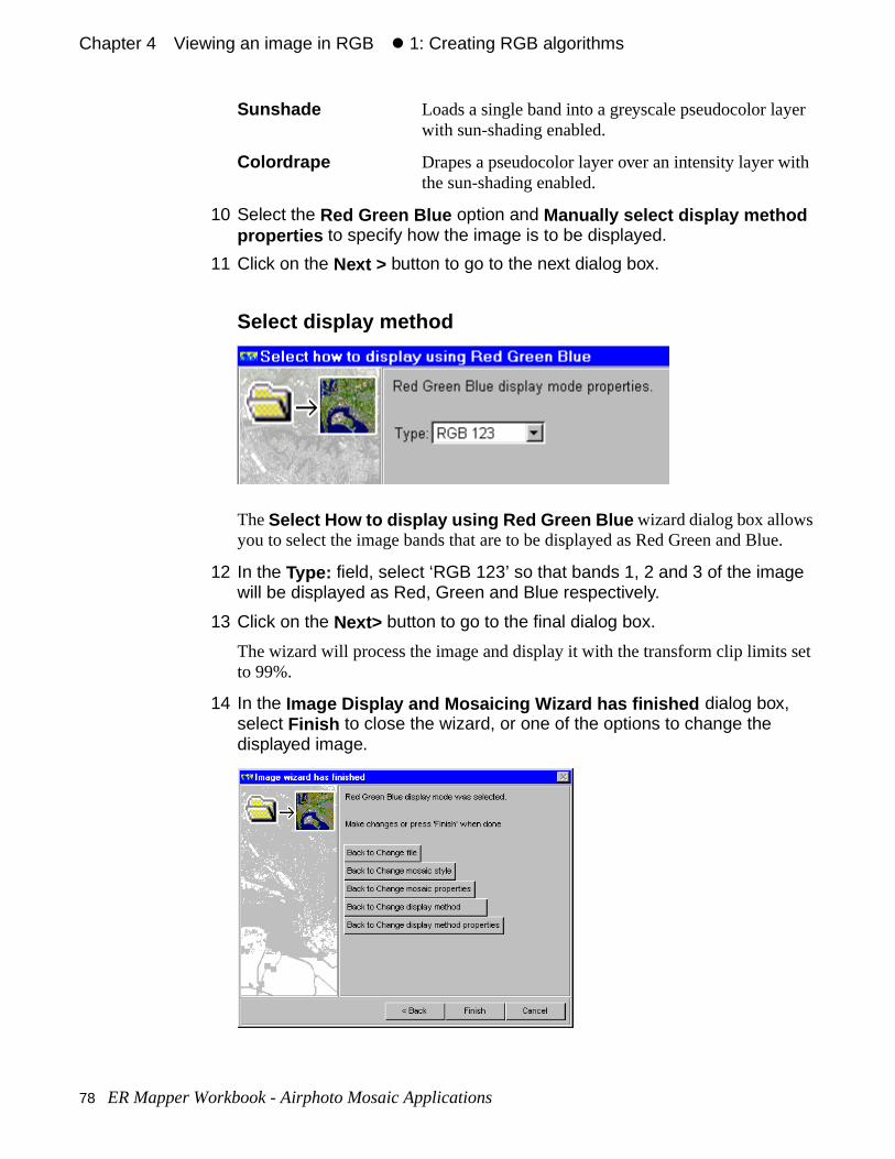
Chapter 4#Viewing an image in RGB#z 1: Creating RGB algorithms
er
th
e.
set
Sunshade Loads a single band into a greyscale pseudocolor laywith sun-shading enabled.
Colordrape Drapes a pseudocolor layer over an intensity layer withe sun-shading enabled.
10 Select the Red Green Blue option and Manually select display method properties to specify how the image is to be displayed.
11 Click on the Next > button to go to the next dialog box.
Select display method
The Select How to display using Red Green Blue wizard dialog box allows you to select the image bands that are to be displayed as Red Green and Blu
12 In the Type: field, select ‘RGB 123’ so that bands 1, 2 and 3 of the image will be displayed as Red, Green and Blue respectively.
13 Click on the Next> button to go to the final dialog box.
The wizard will process the image and display it with the transform clip limits to 99%.
14 In the Image Display and Mosaicing Wizard has finished dialog box, select Finish to close the wizard, or one of the options to change the displayed image.
78 ER Mapper Workbook - Airphoto Mosaic Applications
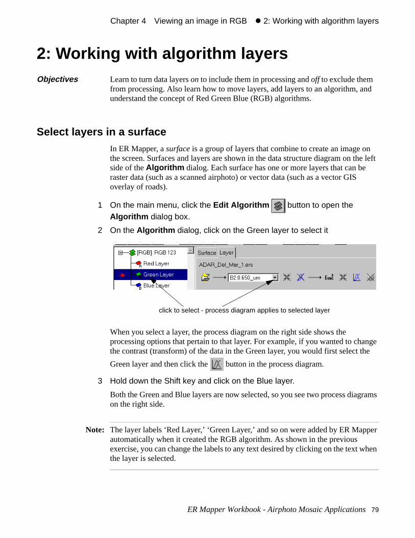
Chapter 4#Viewing an image in RGB#z 2: Working with algorithm layers
n he left
ange he
grams
pper
when
nd
2: Working with algorithm layers
Select layers in a surfaceIn ER Mapper, a surface is a group of layers that combine to create an image othe screen. Surfaces and layers are shown in the data structure diagram on tside of the Algorithm dialog. Each surface has one or more layers that can beraster data (such as a scanned airphoto) or vector data (such as a vector GISoverlay of roads).
1 On the main menu, click the Edit Algorithm button to open the Algorithm dialog box.
2 On the Algorithm dialog, click on the Green layer to select it
When you select a layer, the process diagram on the right side shows the processing options that pertain to that layer. For example, if you wanted to chthe contrast (transform) of the data in the Green layer, you would first select t
Green layer and then click the button in the process diagram.
3 Hold down the Shift key and click on the Blue layer.
Both the Green and Blue layers are now selected, so you see two process diaon the right side.
Note: The layer labels ‘Red Layer,’ ‘Green Layer,’ and so on were added by ER Maautomatically when it created the RGB algorithm. As shown in the previous exercise, you can change the labels to any text desired by clicking on the text the layer is selected.
Objectives Learn to turn data layers on to include them in processing and off to exclude them from processing. Also learn how to move layers, add layers to an algorithm, aunderstand the concept of Red Green Blue (RGB) algorithms.
click to select - process diagram applies to selected layer
ER Mapper Workbook - Airphoto Mosaic Applications 79
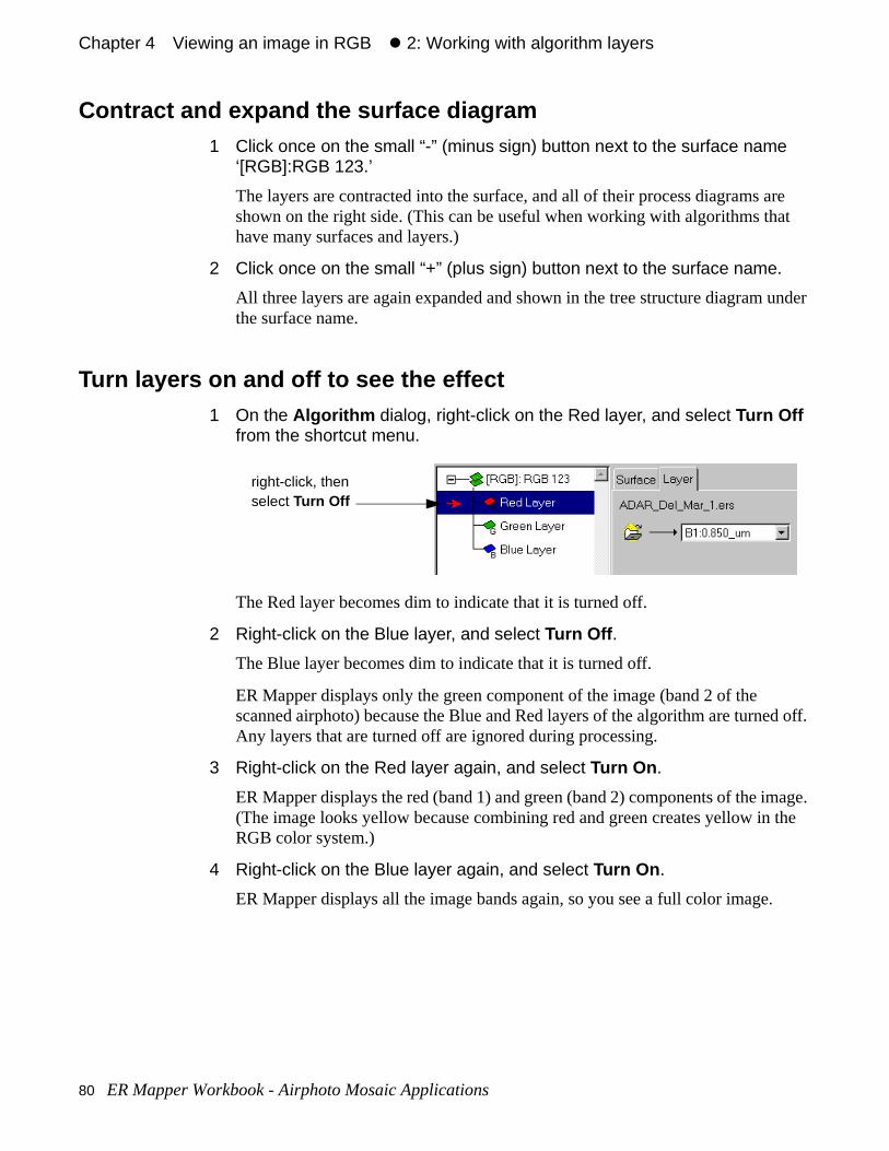
Chapter 4#Viewing an image in RGB#z 2: Working with algorithm layers
re t
under
d off.
age. the
.
Contract and expand the surface diagram1 Click once on the small “-” (minus sign) button next to the surface name
‘[RGB]:RGB 123.’
The layers are contracted into the surface, and all of their process diagrams ashown on the right side. (This can be useful when working with algorithms thahave many surfaces and layers.)
2 Click once on the small “+” (plus sign) button next to the surface name.
All three layers are again expanded and shown in the tree structure diagram the surface name.
Turn layers on and off to see the effect1 On the Algorithm dialog, right-click on the Red layer, and select Turn Off
from the shortcut menu.
The Red layer becomes dim to indicate that it is turned off.
2 Right-click on the Blue layer, and select Turn Off .
The Blue layer becomes dim to indicate that it is turned off.
ER Mapper displays only the green component of the image (band 2 of the scanned airphoto) because the Blue and Red layers of the algorithm are turneAny layers that are turned off are ignored during processing.
3 Right-click on the Red layer again, and select Turn On .
ER Mapper displays the red (band 1) and green (band 2) components of the im(The image looks yellow because combining red and green creates yellow inRGB color system.)
4 Right-click on the Blue layer again, and select Turn On .
ER Mapper displays all the image bands again, so you see a full color image
right-click, thenselect Turn Off
80 ER Mapper Workbook - Airphoto Mosaic Applications
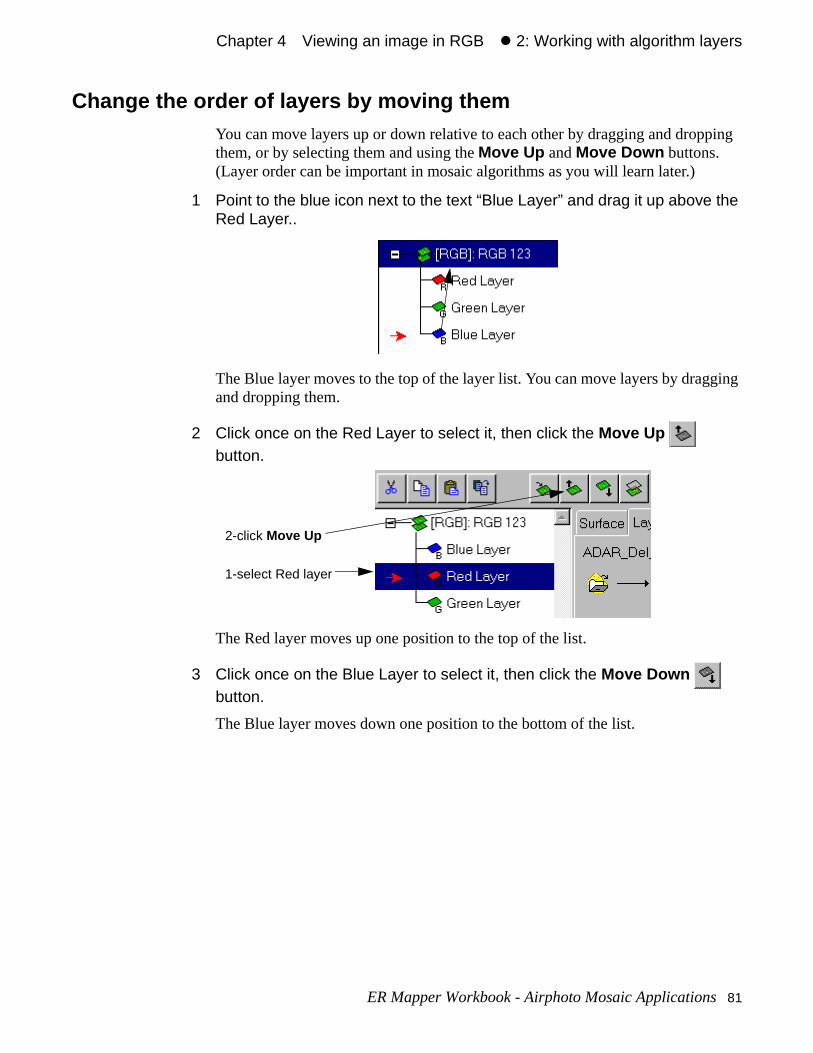
Chapter 4#Viewing an image in RGB#z 2: Working with algorithm layers
ping
ging
Change the order of layers by moving themYou can move layers up or down relative to each other by dragging and dropthem, or by selecting them and using the Move Up and Move Down buttons. (Layer order can be important in mosaic algorithms as you will learn later.)
1 Point to the blue icon next to the text “Blue Layer” and drag it up above the Red Layer..
The Blue layer moves to the top of the layer list. You can move layers by dragand dropping them.
2 Click once on the Red Layer to select it, then click the Move Up button.
The Red layer moves up one position to the top of the list.
3 Click once on the Blue Layer to select it, then click the Move Down button.
The Blue layer moves down one position to the bottom of the list.
1-select Red layer
2-click Move Up
ER Mapper Workbook - Airphoto Mosaic Applications 81
Chapter 4#Viewing an image in RGB#z 3: Loading, adding and changing layers
y er
B B
t
ic
it.)
lso m
3: Loading, adding and changing layers
Load a different dataset into all three layersOne of the great advantages of the ER Mapper’s algorithm concept is that analgorithm can be used as a “template” to apply the same processing to anothdataset. You simply need to load the new dataset.
1 In the process diagram, click on the Load Dataset button.
The Raster Dataset file chooser appears. Move it left so it does not cover theAlgorithm dialog.
2 From the Directories menu, select the path ending with the text \examples .
3 Double-click to open the directory named ‘Shared_Data.’
4 Click once on the dataset named ‘Airphoto.ers.’
5 Click the Apply button.
The dataset is loaded into all three layers in the algorithm.
ER Mapper displays an airphoto of downtown San Diego, California as an RGcolor composite image. This demonstrates that you can open any existing RGalgorithm and simply load a different dataset to view in RGB also.
6 On the main ER Mapper menu, click the 99% Contrast Enhancement button to improve the image contrast.
About the OK and Apply buttons
• If all three layers contain the same dataset (as in this case), Apply and OK load thenew dataset into all three layers automatically. (Apply and OK are the same excepthat Apply leaves the dialog open and OK closes it.)
• If you want to load a dataset into only the currently selected layer, use Apply thislayer only or OK this layer only . This is often useful when creating mosaalgorithms as you will see later. (Apply this layer only and OK this layer onlyare the same except that the first leaves the dialog open and the other closes
• Double-clicking on a dataset name in the file chooser is the same as clicking OK.
Objectives Learn to load a dataset into a specific layer or set of layers in an algorithm. Alearn to add and delete layers, change the layer type, and change the algorithColor Mode.
82 ER Mapper Workbook - Airphoto Mosaic Applications
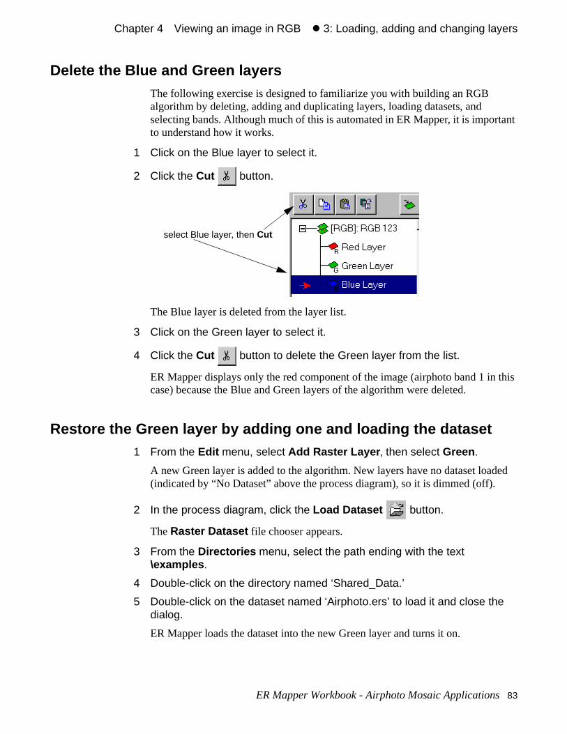
Chapter 4#Viewing an image in RGB#z 3: Loading, adding and changing layers
tant
this
ded
Delete the Blue and Green layersThe following exercise is designed to familiarize you with building an RGB algorithm by deleting, adding and duplicating layers, loading datasets, and selecting bands. Although much of this is automated in ER Mapper, it is importo understand how it works.
1 Click on the Blue layer to select it.
2 Click the Cut button.
The Blue layer is deleted from the layer list.
3 Click on the Green layer to select it.
4 Click the Cut button to delete the Green layer from the list.
ER Mapper displays only the red component of the image (airphoto band 1 incase) because the Blue and Green layers of the algorithm were deleted.
Restore the Green layer by adding one and loading the dataset1 From the Edit menu, select Add Raster Layer , then select Green .
A new Green layer is added to the algorithm. New layers have no dataset loa(indicated by “No Dataset” above the process diagram), so it is dimmed (off).
2 In the process diagram, click the Load Dataset button.
The Raster Dataset file chooser appears.
3 From the Directories menu, select the path ending with the text \examples .
4 Double-click on the directory named ‘Shared_Data.’
5 Double-click on the dataset named ‘Airphoto.ers’ to load it and close the dialog.
ER Mapper loads the dataset into the new Green layer and turns it on.
select Blue layer, then Cut
ER Mapper Workbook - Airphoto Mosaic Applications 83
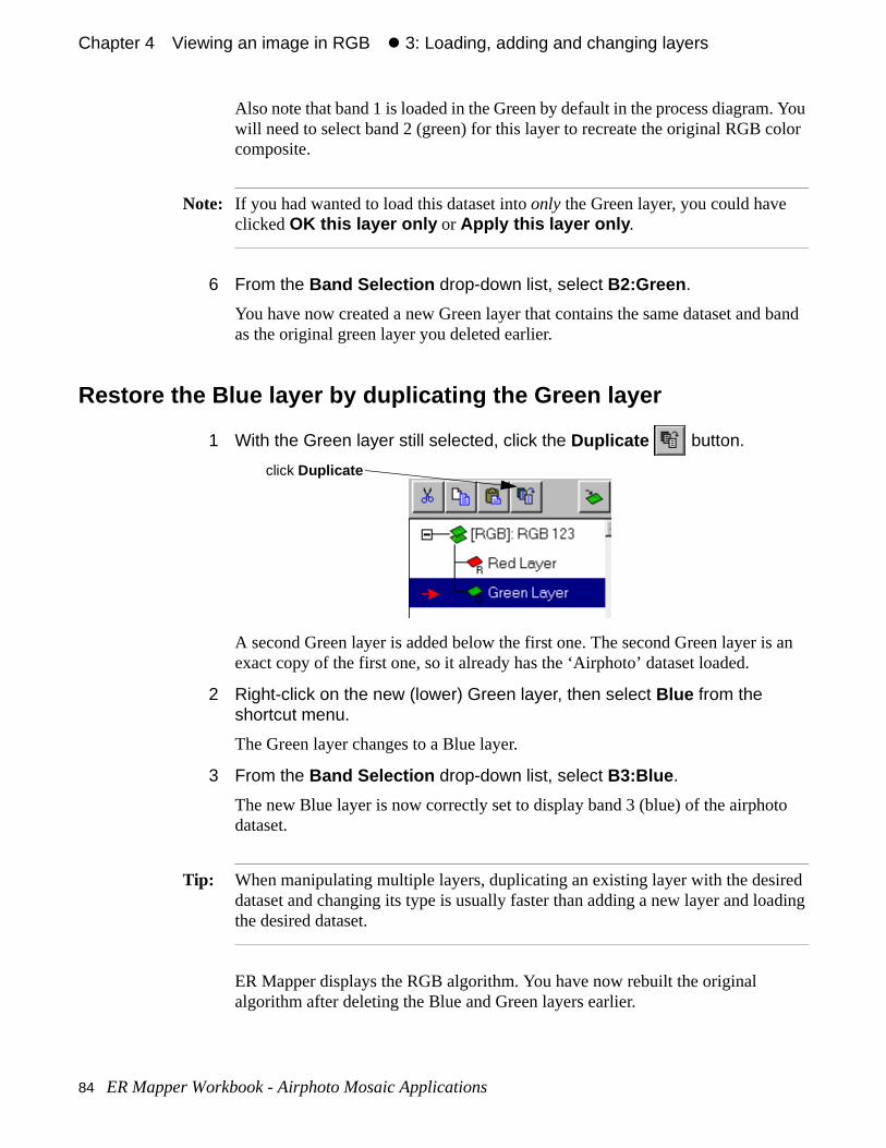
Chapter 4#Viewing an image in RGB#z 3: Loading, adding and changing layers
. You olor
band
s an
to
red ading
Also note that band 1 is loaded in the Green by default in the process diagramwill need to select band 2 (green) for this layer to recreate the original RGB ccomposite.
Note: If you had wanted to load this dataset into only the Green layer, you could have clicked OK this layer only or Apply this layer only .
6 From the Band Selection drop-down list, select B2:Green .
You have now created a new Green layer that contains the same dataset andas the original green layer you deleted earlier.
Restore the Blue layer by duplicating the Green layer
1 With the Green layer still selected, click the Duplicate button.
A second Green layer is added below the first one. The second Green layer iexact copy of the first one, so it already has the ‘Airphoto’ dataset loaded.
2 Right-click on the new (lower) Green layer, then select Blue from the shortcut menu.
The Green layer changes to a Blue layer.
3 From the Band Selection drop-down list, select B3:Blue .
The new Blue layer is now correctly set to display band 3 (blue) of the airphodataset.
Tip: When manipulating multiple layers, duplicating an existing layer with the desidataset and changing its type is usually faster than adding a new layer and lothe desired dataset.
ER Mapper displays the RGB algorithm. You have now rebuilt the original algorithm after deleting the Blue and Green layers earlier.
click Duplicate
84 ER Mapper Workbook - Airphoto Mosaic Applications
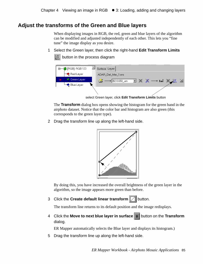
Chapter 4#Viewing an image in RGB#z 3: Loading, adding and changing layers
hm
the
the
Adjust the transforms of the Green and Blue layersWhen displaying images in RGB, the red, green and blue layers of the algoritcan be modified and adjusted independently of each other. This lets you “finetune” the image display as you desire.
1 Select the Green layer, then click the right-hand Edit Transform Limits
button in the process diagram
The Transform dialog box opens showing the histogram for the green band inairphoto dataset. Notice that the color bar and histogram are also green (thiscorresponds to the green layer type).
2 Drag the transform line up along the left-hand side.
By doing this, you have increased the overall brightness of the green layer inalgorithm, so the image appears more green than before.
3 Click the Create default linear transform button.
The transform line returns to its default position and the image redisplays.
4 Click the Move to next blue layer in surface button on the Transform dialog.
ER Mapper automatically selects the Blue layer and displays its histogram.)
5 Drag the transform line up along the left-hand side.
select Green layer, click Edit Transform Limits button
ER Mapper Workbook - Airphoto Mosaic Applications 85
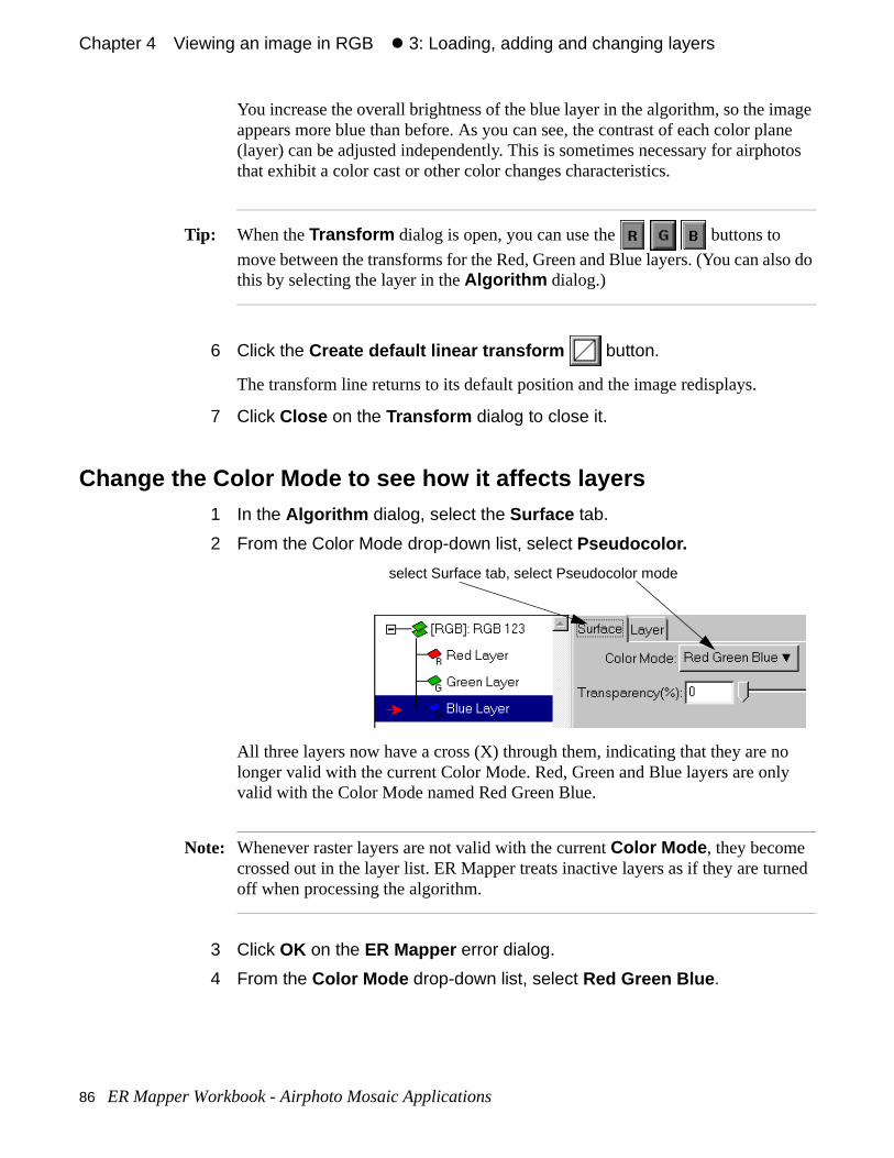
Chapter 4#Viewing an image in RGB#z 3: Loading, adding and changing layers
age ane otos
lso do
o y
rned
You increase the overall brightness of the blue layer in the algorithm, so the imappears more blue than before. As you can see, the contrast of each color pl(layer) can be adjusted independently. This is sometimes necessary for airphthat exhibit a color cast or other color changes characteristics.
Tip: When the Transform dialog is open, you can use the buttons to
move between the transforms for the Red, Green and Blue layers. (You can athis by selecting the layer in the Algorithm dialog.)
6 Click the Create default linear transform button.
The transform line returns to its default position and the image redisplays.
7 Click Close on the Transform dialog to close it.
Change the Color Mode to see how it affects layers1 In the Algorithm dialog, select the Surface tab.
2 From the Color Mode drop-down list, select Pseudocolor.
All three layers now have a cross (X) through them, indicating that they are nlonger valid with the current Color Mode. Red, Green and Blue layers are onlvalid with the Color Mode named Red Green Blue.
Note: Whenever raster layers are not valid with the current Color Mode , they become crossed out in the layer list. ER Mapper treats inactive layers as if they are tuoff when processing the algorithm.
3 Click OK on the ER Mapper error dialog.
4 From the Color Mode drop-down list, select Red Green Blue .
select Surface tab, select Pseudocolor mode
86 ER Mapper Workbook - Airphoto Mosaic Applications
Chapter 4#Viewing an image in RGB#z 4: Labelling and saving the algorithm
m,
.)
Note: Black and white airphotos usually have only one band of data. To display theyou use the Color Mode named Pseudocolor, a layer of type Pseudo, and the‘greyscale’ Color Table to create black and white image.
4: Labelling and saving the algorithm
Enter a description for the entire algorithm1 In the Algorithm dialog, select the text in the Description text field (it
currently reads ‘RGB 321’).
(To select the text, either drag through it, or triple-click to select the entire line
2 Type the following text, then press Enter or Return on your keyboard:
Airphoto in RGB
This text now becomes a brief description for the entire algorithm.
Save the processing steps to an algorithm file on disk1 From the File menu (on the main menu), select Save As... .
The Save Algorithm file chooser dialog opens.
2 From the Directories menu, select the path ending with the text examples\ . (The portion of the path name preceding it is specific to your site.)
3 Double-click on the directory named ‘airphoto_training’ to open it.
4 In the Save As: text field, click to place the cursor, then type the following name for the algorithm file:
Airphoto_in_RGB
5 Click the Apply button to save the algorithm and leave the dialog open.
Your RGB algorithm is now saved to an algorithm file on disk.
Objectives Learn to specify description labels, titles, and comments for an algorithm, andsave the algorithm processing steps to a file so you can view it later.
ER Mapper Workbook - Airphoto Mosaic Applications 87
Chapter 4#Viewing an image in RGB#z 4: Labelling and saving the algorithm
s
Add comments to the algorithm1 On the Save Algorithm dialog, click the Comments... button.
2 In the comments dialog, type the following information:
This algorithm displays the airphoto as an RGB
algorithm. A 99% autoclip transform is used to increase
image contrast.
3 Click OK on the comments dialog to save your comments.
4 Click Cancel on the Save Algorithm dialog close it.
Close the image window and the Algorithm dialog1 Close the image window:
• For Windows, click the Close button in the upper-right window corner.
2 On the Algorithm dialog, click the Close button.
Only the ER Mapper main menu is now open on the screen.
• Open a dataset directly and have ER Mapper create a display algorithm
• Use the Image Display and Mosaic Wizard to display an RGB algorithm
• Understand the red, green and blue layers in an RGB algorithm
• Delete, add and change layers in an algorithm
• Use transforms to adjust the RGB color contrast
What you learned...
After completing these exercises, you know how to perform the following taskin ER Mapper:
88 ER Mapper Workbook - Airphoto Mosaic Applications
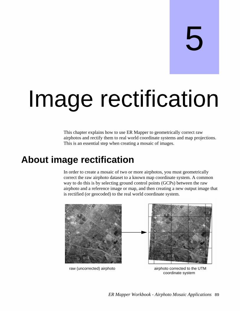
ons.
on
e that
5
Image rectificationThis chapter explains how to use ER Mapper to geometrically correct raw airphotos and rectify them to real world coordinate systems and map projectiThis is an essential step when creating a mosaic of images.
About image rectificationIn order to create a mosaic of two or more airphotos, you must geometrically correct the raw airphoto dataset to a known map coordinate system. A commway to do this is by selecting ground control points (GCPs) between the raw airphoto and a reference image or map, and then creating a new output imagis rectified (or geocoded) to the real world coordinate system.
raw (uncorrected) airphoto airphoto corrected to the UTMcoordinate system
ER Mapper Workbook - Airphoto Mosaic Applications 89
Chapter 5 Image rectification z About image rectification
ch or
r eded to
t:
to
wnnotherset, aown
pper. OQ)
apper, rs are
r use
A ground control point (GCP) is a point on the earth’s surface where both image coordinates (measured in rows and columns) and map coordinates (measured in degrees of latitude and longitude, meters, or feet) can be identified. Rectification is the process of using GCPs to transform the geometry of an image so that eapixel corresponds to a position in a real world coordinate system (such a UTMState Plane map projection). This process is sometimes called “geocoding” o“rubbersheeting” because the image data are stretched or compressed as nealign with a real world map grid or coordinate system.
To perform a control point rectification, you need a raw and reference datase
• The raw dataset is simply a digitized airphoto that has been imported inER Mapper
• The reference dataset is any other dataset, hardcopy map, or set of knocoordinate points that can be used to correct the raw dataset. You can use aairphoto or image that has already been rectified, a geocoded vector datahardcopy map mounted on a digitizing table, or GPS survey points of knfeatures in your image (such as buildings or road intersections).
Note: Some airphoto datasets have already been rectified before import into ER MaThese include orthorectified datasets such as the USGS Digital Ortho Quad (Dseries and others. In this case, you do not need to rectify the dataset in ER Myou only need to make sure the proper datum, projection, and other parametespecified (usually using the dataset header editor).
Note: Orthorectification , which is described in the next chapter, is a more accurate method for geocoding images. For this reason, it is generally recommended fowith airphotos.
90 ER Mapper Workbook - Airphoto Mosaic Applications
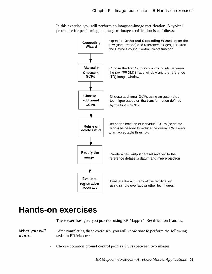
Chapter 5#Image rectification#z Hands-on exercises
In this exercise, you will perform an image-to-image rectification. A typical procedure for performing an image-to-image rectification is as follows:
Hands-on exercisesThese exercises give you practice using ER Mapper’s Rectification features.
• Choose common ground control points (GCPs) between two images
What you will learn...
After completing these exercises, you will know how to perform the following tasks in ER Mapper:
Open the Ortho and Geocoding Wizard , enter the
Choose the first 4 ground control points between
Geocoding
Choose 4GCPs
Chooseadditional
GCPs
raw (uncorrected) and reference images, and start
the raw (FROM) image window and the reference(TO) image window
Choose additional GCPs using an automatedtechnique based on the transformation defined
the Define Ground Control Points function
Refine the location of individual GCPs (or delete
Create a new output dataset rectified to the
Refine ordelete GCPs
Rectify theimage
Evaluateregistration
accuracy
GCPs) as needed to reduce the overall RMS error
reference dataset’s datum and map projection
Evaluate the accuracy of the rectificationusing simple overlays or other techniques
to an acceptable threshold
Wizard
Manually
by the first 4 GCPs
ER Mapper Workbook - Airphoto Mosaic Applications 91
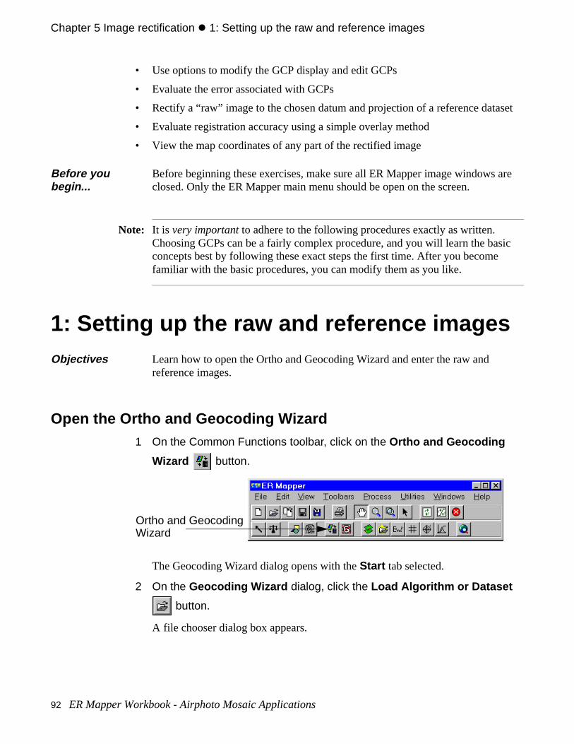
Chapter 5 Image rectification z 1: Setting up the raw and reference images
set
sic
are
• Use options to modify the GCP display and edit GCPs
• Evaluate the error associated with GCPs
• Rectify a “raw” image to the chosen datum and projection of a reference data
• Evaluate registration accuracy using a simple overlay method
• View the map coordinates of any part of the rectified image
Note: It is very important to adhere to the following procedures exactly as written. Choosing GCPs can be a fairly complex procedure, and you will learn the baconcepts best by following these exact steps the first time. After you becomefamiliar with the basic procedures, you can modify them as you like.
1: Setting up the raw and reference images
Open the Ortho and Geocoding Wizard1 On the Common Functions toolbar, click on the Ortho and Geocoding
Wizard button.
The Geocoding Wizard dialog opens with the Start tab selected.
2 On the Geocoding Wizard dialog, click the Load Algorithm or Dataset
button.
A file chooser dialog box appears.
Before you begin...
Before beginning these exercises, make sure all ER Mapper image windows closed. Only the ER Mapper main menu should be open on the screen.
Objectives Learn how to open the Ortho and Geocoding Wizard and enter the raw and reference images.
Ortho and GeocodingWizard
92 ER Mapper Workbook - Airphoto Mosaic Applications
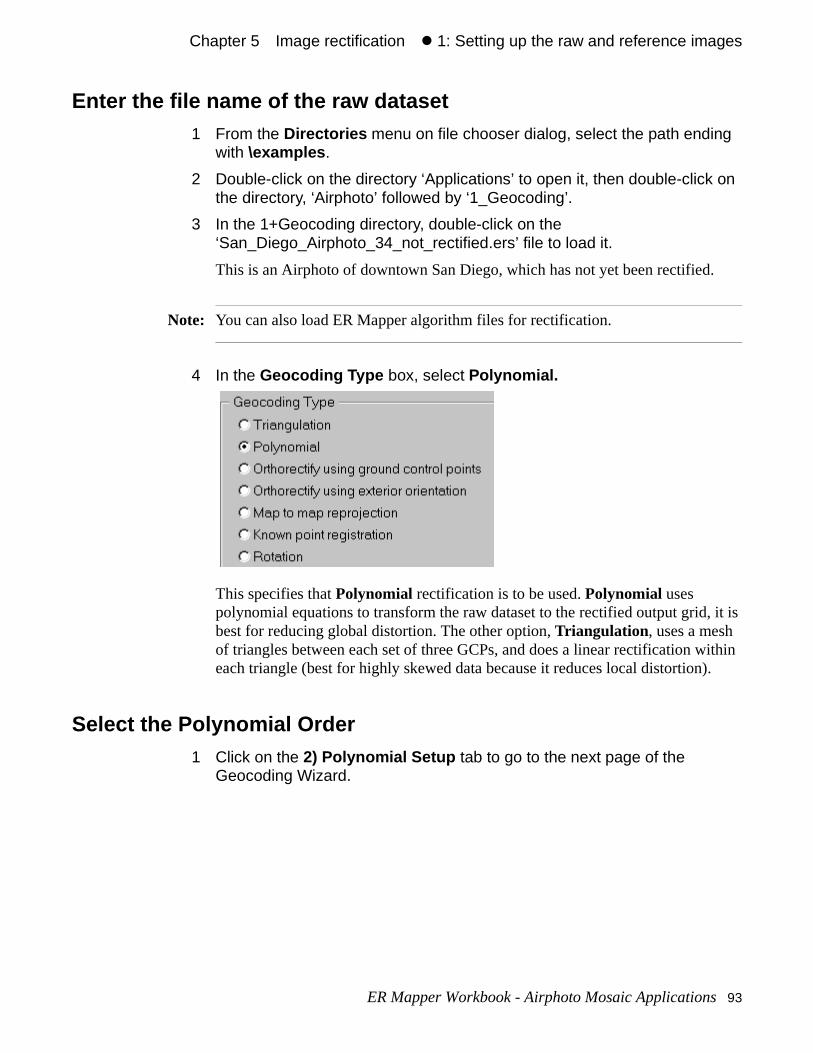
Chapter 5#Image rectification#z 1: Setting up the raw and reference images
it is
ithin ).
Enter the file name of the raw dataset1 From the Directories menu on file chooser dialog, select the path ending
with \examples .
2 Double-click on the directory ‘Applications’ to open it, then double-click on the directory, ‘Airphoto’ followed by ‘1_Geocoding’.
3 In the 1+Geocoding directory, double-click on the ‘San_Diego_Airphoto_34_not_rectified.ers’ file to load it.
This is an Airphoto of downtown San Diego, which has not yet been rectified.
Note: You can also load ER Mapper algorithm files for rectification.
4 In the Geocoding Type box, select Polynomial.
This specifies that Polynomial rectification is to be used. Polynomial uses polynomial equations to transform the raw dataset to the rectified output grid,best for reducing global distortion. The other option, Triangulation , uses a mesh of triangles between each set of three GCPs, and does a linear rectification weach triangle (best for highly skewed data because it reduces local distortion
Select the Polynomial Order1 Click on the 2) Polynomial Setup tab to go to the next page of the
Geocoding Wizard.
ER Mapper Workbook - Airphoto Mosaic Applications 93
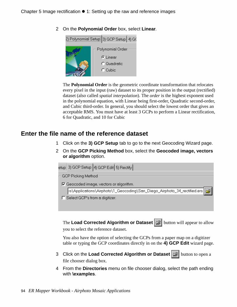
Chapter 5 Image rectification z 1: Setting up the raw and reference images
s ied) der, s an tion,
er
2 On the Polynomial Order box, select Linear .
The Polynomial Order is the geometric coordinate transformation that relocateevery pixel in the input (raw) dataset to its proper position in the output (rectifdataset (also called spatial interpolation). The order is the highest exponent usedin the polynomial equation, with Linear being first-order, Quadratic second-orand Cubic third-order. In general, you should select the lowest order that giveacceptable RMS. You must have at least 3 GCPs to perform a Linear rectifica6 for Quadratic, and 10 for Cubic
Enter the file name of the reference dataset1 Click on the 3) GCP Setup tab to go to the next Geocoding Wizard page.
2 On the GCP Picking Method box, select the Geocoded image, vectors or algorithm option.
The Load Corrected Algorithm or Dataset button will appear to allow
you to select the reference dataset.
You also have the option of selecting the GCPs from a paper map on a digitiztable or typing the GCP coordinates directly in on the 4) GCP Edit wizard page.
3 Click on the Load Corrected Algorithm or Dataset button to open a
file chooser dialog box.
4 From the Directories menu on file chooser dialog, select the path ending with \examples .
94 ER Mapper Workbook - Airphoto Mosaic Applications
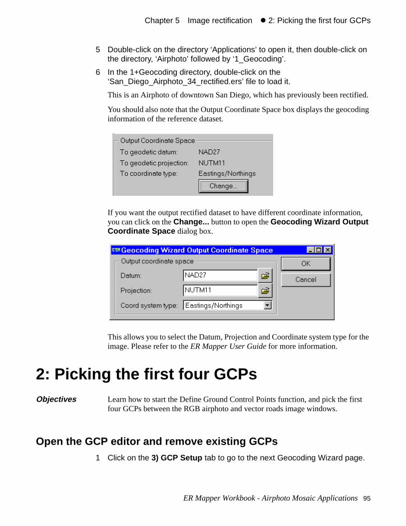
Chapter 5#Image rectification#z 2: Picking the first four GCPs
ied.
oding
n,
r the
st
5 Double-click on the directory ‘Applications’ to open it, then double-click on the directory, ‘Airphoto’ followed by ‘1_Geocoding’.
6 In the 1+Geocoding directory, double-click on the ‘San_Diego_Airphoto_34_rectified.ers’ file to load it.
This is an Airphoto of downtown San Diego, which has previously been rectif
You should also note that the Output Coordinate Space box displays the geocinformation of the reference dataset.
If you want the output rectified dataset to have different coordinate informatioyou can click on the Change... button to open the Geocoding Wizard Output Coordinate Space dialog box.
This allows you to select the Datum, Projection and Coordinate system type foimage. Please refer to the ER Mapper User Guide for more information.
2: Picking the first four GCPs
Open the GCP editor and remove existing GCPs1 Click on the 3) GCP Setup tab to go to the next Geocoding Wizard page.
Objectives Learn how to start the Define Ground Control Points function, and pick the firfour GCPs between the RGB airphoto and vector roads image windows.
ER Mapper Workbook - Airphoto Mosaic Applications 95
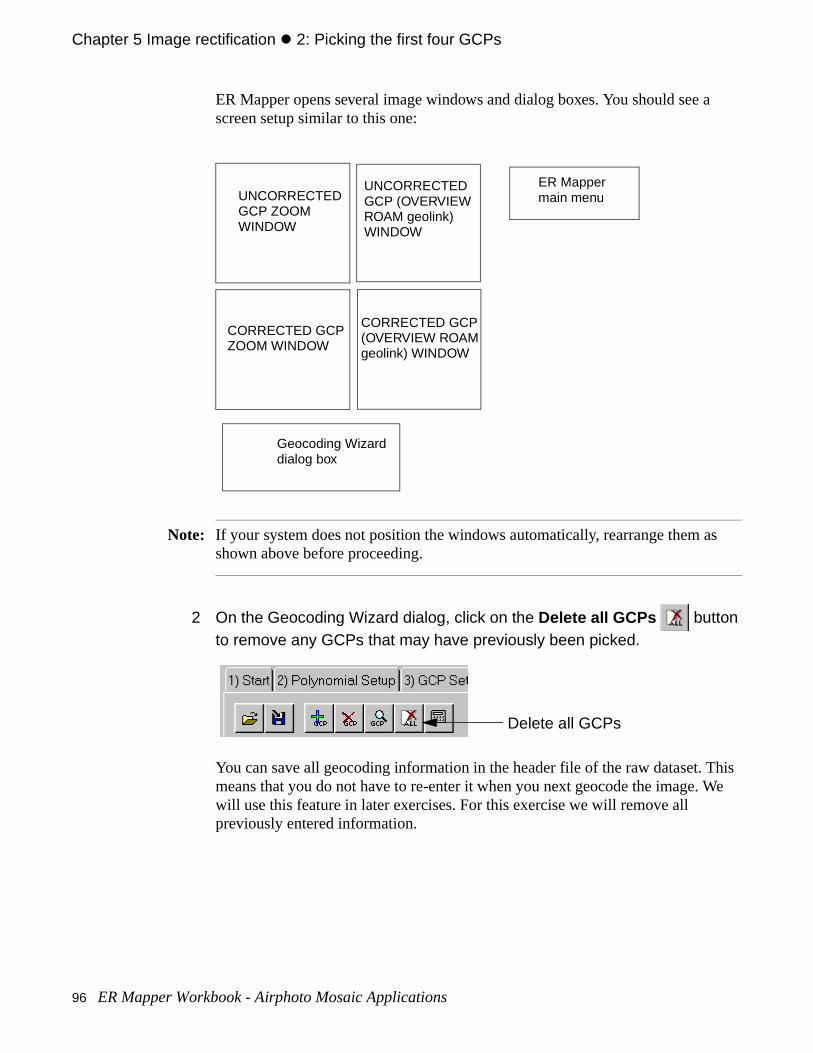
Chapter 5 Image rectification z 2: Picking the first four GCPs
a
s
This We
ER Mapper opens several image windows and dialog boxes. You should see screen setup similar to this one:
Note: If your system does not position the windows automatically, rearrange them ashown above before proceeding.
2 On the Geocoding Wizard dialog, click on the Delete all GCPs button to remove any GCPs that may have previously been picked.
You can save all geocoding information in the header file of the raw dataset. means that you do not have to re-enter it when you next geocode the image.will use this feature in later exercises. For this exercise we will remove all previously entered information.
ER Mappermain menu
Geocoding Wizarddialog box
UNCORRECTEDGCP ZOOMWINDOW
CORRECTED GCPZOOM WINDOW
UNCORRECTEDGCP (OVERVIEWROAM geolink)WINDOW
CORRECTED GCP(OVERVIEW ROAMgeolink) WINDOW
Delete all GCPs
96 ER Mapper Workbook - Airphoto Mosaic Applications
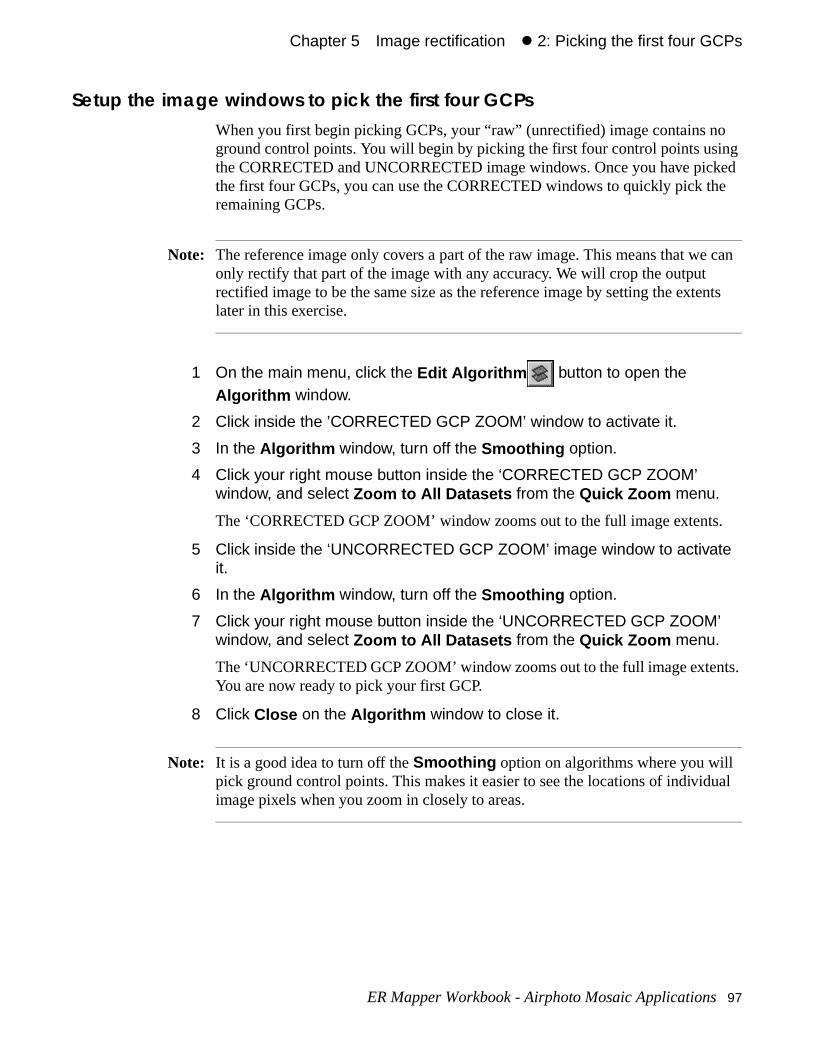
Chapter 5#Image rectification#z 2: Picking the first four GCPs
o ng ked e
can
nts
.
ts.
ual
Setup the image windows to pick the first four GCPsWhen you first begin picking GCPs, your “raw” (unrectified) image contains nground control points. You will begin by picking the first four control points usithe CORRECTED and UNCORRECTED image windows. Once you have picthe first four GCPs, you can use the CORRECTED windows to quickly pick thremaining GCPs.
Note: The reference image only covers a part of the raw image. This means that weonly rectify that part of the image with any accuracy. We will crop the output rectified image to be the same size as the reference image by setting the extelater in this exercise.
1 On the main menu, click the Edit Algorithm button to open the Algorithm window.
2 Click inside the ’CORRECTED GCP ZOOM’ window to activate it.
3 In the Algorithm window, turn off the Smoothing option.
4 Click your right mouse button inside the ‘CORRECTED GCP ZOOM’ window, and select Zoom to All Datasets from the Quick Zoom menu.
The ‘CORRECTED GCP ZOOM’ window zooms out to the full image extents
5 Click inside the ‘UNCORRECTED GCP ZOOM’ image window to activate it.
6 In the Algorithm window, turn off the Smoothing option.
7 Click your right mouse button inside the ‘UNCORRECTED GCP ZOOM’ window, and select Zoom to All Datasets from the Quick Zoom menu.
The ‘UNCORRECTED GCP ZOOM’ window zooms out to the full image extenYou are now ready to pick your first GCP.
8 Click Close on the Algorithm window to close it.
Note: It is a good idea to turn off the Smoothing option on algorithms where you will pick ground control points. This makes it easier to see the locations of individimage pixels when you zoom in closely to areas.
ER Mapper Workbook - Airphoto Mosaic Applications 97
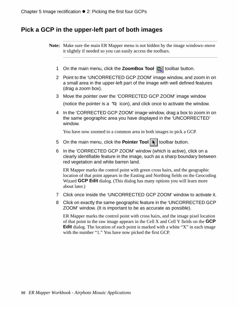
Chapter 5 Image rectification z 2: Picking the first four GCPs
ove
ic
tion
ge
Pick a GCP in the upper-left part of both images
Note: Make sure the main ER Mapper menu is not hidden by the image windows–mit slightly if needed so you can easily access the toolbars.
1 On the main menu, click the ZoomBox Tool toolbar button.
2 Point to the ‘UNCORRECTED GCP ZOOM’ image window, and zoom in on a small area in the upper-left part of the image with well defined features (drag a zoom box).
3 Move the pointer over the ‘CORRECTED GCP ZOOM’ image window
(notice the pointer is a icon), and click once to activate the window.
4 In the ‘CORRECTED GCP ZOOM’ image window, drag a box to zoom in on the same geographic area you have displayed in the ‘UNCORRECTED’ window.
You have now zoomed to a common area in both images to pick a GCP.
5 On the main menu, click the Pointer Tool toolbar button.
6 In the ‘CORRECTED GCP ZOOM’ window (which is active), click on a clearly identifiable feature in the image, such as a sharp boundary between red vegetation and white barren land.
ER Mapper marks the control point with green cross hairs, and the geographlocation of that point appears in the Easting and Northing fields on the GeocodingWizard GCP Edit dialog. (This dialog has many options you will learn more about later.)
7 Click once inside the ‘UNCORRECTED GCP ZOOM’ window to activate it.
8 Click on exactly the same geographic feature in the ‘UNCORRECTED GCP ZOOM’ window. (It is important to be as accurate as possible).
ER Mapper marks the control point with cross hairs, and the image pixel locaof that point in the raw image appears in the Cell X and Cell Y fields on the GCP Edit dialog. The location of each point is marked with a white “X” in each imawith the number “1.” You have now picked the first GCP.
98 ER Mapper Workbook - Airphoto Mosaic Applications
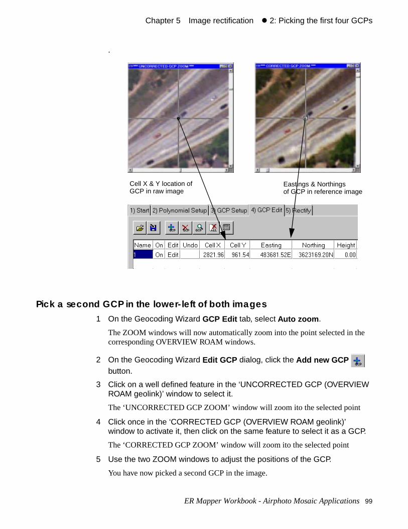
Chapter 5#Image rectification#z 2: Picking the first four GCPs
e
.
Pick a second GCP in the lower-left of both images1 On the Geocoding Wizard GCP Edit tab, select Auto zoom .
The ZOOM windows will now automatically zoom into the point selected in thcorresponding OVERVIEW ROAM windows.
2 On the Geocoding Wizard Edit GCP dialog, click the Add new GCP button.
3 Click on a well defined feature in the ‘UNCORRECTED GCP (OVERVIEW ROAM geolink)’ window to select it.
The ‘UNCORRECTED GCP ZOOM’ window will zoom ito the selected point
4 Click once in the ‘CORRECTED GCP (OVERVIEW ROAM geolink)’ window to activate it, then click on the same feature to select it as a GCP.
The ‘CORRECTED GCP ZOOM’ window will zoom ito the selected point
5 Use the two ZOOM windows to adjust the positions of the GCP.
You have now picked a second GCP in the image.
Cell X & Y location ofGCP in raw image
Eastings & Northingsof GCP in reference image
ER Mapper Workbook - Airphoto Mosaic Applications 99
Chapter 5 Image rectification z 2: Picking the first four GCPs
the
as
ys ) n the ase ng the
D’
asier,
mage he CPs,
are GCP
s of a 5.00
trol s for
Pick two more GCPs in the upper- and lower-right1 Following the steps from the previous section, pick a GCP near the upper-
right and lower-right corners of the images.
Tip: When picking the first four GCPs, it is best to pick them in the four corners ofCORRECTED image (if this is possible). This will make the Calculate from point function you will use next as accurate as possible. (In this case there wocean in the lower-left, so you picked a point in the closest area possible.)
Once you have picked the first four GCPs, notice that ER Mapper now displavalues in the ‘RMS’ field on the GCP Edit dialog. The Root Mean Square (RMSerror is a measurement of the accuracy of the GCP in this image expressed iimage’s pixel size. (An RMS of 1.00 would be 80 meter positional error in the cof the Landsat MSS data used here.) If you have done an accurate job selectifirst four GCPs, the RMS should be one or less.
When an RMS can be calculated, ER Mapper can now use the coefficients generated from the first four points to “predict” the location of ‘UNCORRECTE(raw) points when you pick additional points in the ‘CORRECTED’ (rectified) image. This feature makes selection of the remaining points much faster and eand you will use it next.
About RMS errors
GCPs are used to compute a mathematical transformation to rectify the raw ito a geographic frame of reference (in this case, the UTM map projection of tvector dataset). Using coordinate transform coefficients computed from the Git is possible to model geometric distortions in the raw airphoto.
A common way to measure this distortion is by computing the root mean squ(RMS) error for each control point. This value represents the accuracy of the in the image. ER Mapper is able to compute the RMS error when you have selected at least four control points.
The RMS error is expressed in the dataset’s pixel size (or corresponding unitvector dataset). This raw airphoto has a pixel size of 2 meters, so an RMS ofrepresents a 10 meter positional error. GCPs with lower RMS errors are moreaccurate than ones with higher errors, and you should strive to pick your conpoints with the lowest possible RMS error. If you have control points with higherrors, you can try to adjust them to decrease the error, or delete them. (Stepadjusting GCPs will be covered later.)
100 ER Mapper Workbook - Airphoto Mosaic Applications
Chapter 5#Image rectification#z 3: Picking additional GCPs in the images
ED’
ic
ion
alue
nt”
3: Picking additional GCPs in the images
After you have picked your first four GCPs, ER Mapper can use the resulting geometric model to predict where a point picked in the reference ‘CORRECTimage will be located in the raw ‘UNCORRECTED’ image. Based on this, youwill use a different technique for picking the rest of your control points for thisexercise.
Pick additional GCPs using the Corrected GCP Overview window
1 On the main menu, click the Set Pointer mode button (if needed).
2 If needed, activate the ‘CORRECTED GCP (OVERVIEW ROAM geolink)’ window by clicking in it.
3 On the Geocoding Wizard Edit GCP dialog, click the Add GCP button.
4 In the ‘CORRECTED GCP (OVERVIEW ROAM geolink)’ window, click on a well defined feature near the center of the image.
ER Mapper marks the control point with cross hairs, and enters the geographlocation of GCP #5 in the TO Easting and Northing fields. The ‘CORRECTED GCP ZOOM’ window zooms into the point for you to adjust its position.
5 In the Geocoding Wizard GCP Edit dialog, click the Calculate from point
button.
ER Mapper automatically enters values in Cell X and Cell Y fields–this is the “predicted” location of GCP #5 in the FROM image.
Notice that the new GCP #5 has an RMS error of zero. Since it’s location is computed from the existing points, it adds no new information to the rectificatmodel (and is therefore not yet a true GCP). Next you need to “fine tune” the location of the point in the ZOOM windows to make it a true GCP.
6 Click once in one of the ZOOM windows to activate it, then click on the GCP in the image. Adjust its position if necessary.
ER Mapper repositions GCP #5 to the new position, and calculates an RMS vto display in the Geocoding Wizard GCP Edit dialog box.
You have now picked a fifth GCP using the “predict FROM points” technique.
Objectives Learn how to use the overview image window and “Calculate uncorrected poifunction to help speed and simplify picking of the remaining control points.
ER Mapper Workbook - Airphoto Mosaic Applications 101
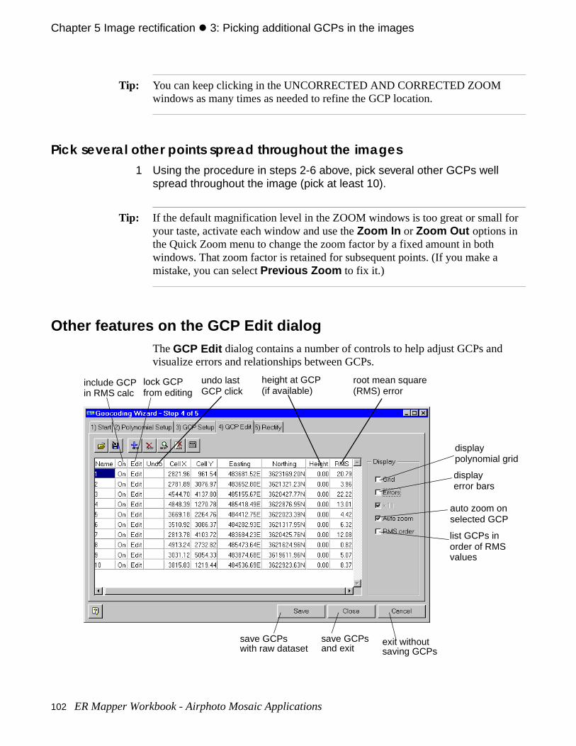
Chapter 5 Image rectification z 3: Picking additional GCPs in the images
r
Tip: You can keep clicking in the UNCORRECTED AND CORRECTED ZOOM windows as many times as needed to refine the GCP location.
Pick several other points spread throughout the images1 Using the procedure in steps 2-6 above, pick several other GCPs well
spread throughout the image (pick at least 10).
Tip: If the default magnification level in the ZOOM windows is too great or small foyour taste, activate each window and use the Zoom In or Zoom Out options in the Quick Zoom menu to change the zoom factor by a fixed amount in both windows. That zoom factor is retained for subsequent points. (If you make a mistake, you can select Previous Zoom to fix it.)
Other features on the GCP Edit dialogThe GCP Edit dialog contains a number of controls to help adjust GCPs and visualize errors and relationships between GCPs.
save GCPswith raw dataset
save GCPsand exit
exit withoutsaving GCPs
displaypolynomial grid
displayerror bars
auto zoom onselected GCP
list GCPs inorder of RMSvalues
include GCPin RMS calc
lock GCPfrom editing
undo lastGCP click
root mean square(RMS) error
height at GCP(if available)
102 ER Mapper Workbook - Airphoto Mosaic Applications
Chapter 5#Image rectification#z 3: Picking additional GCPs in the images
to
ding n a nal en t is
CP
1 In the Geocoding Wizard GCP Edit dialog, click on any GCP number under the ‘Name’ column.
ER Mapper moves the crosshairs to highlight that point in all the ‘OVERVIEWROAM’ and ‘ZOOM’ windows.
2 Turn off the Auto Zoom option.
3 Click on any GCP number under the ‘Name’ column.
ER Mapper moves the crosshairs to highlight that point in the ‘OVERVIEW ROAM’ windows, but not the ‘ZOOM’ windows.
4 Click on the Zoom to current GCP button.
ER Mapper zooms into the selected GCP in the “ZOOM’ windows.
5 Turn on the Auto Zoom option.
View the contribution of a single GCP to the RMS errors1 In the GCP Edit dialog, click on the number under the ‘Name’ field for a
GCP with a high RMS error value. (You can scroll the GCP list or make the GCP Edit dialog bigger to see more points at once.)
ER Mapper highlights that GCP location in the large ‘TO’ window, and zoomsthat point on the smaller zoom windows. This is now the active GCP, so any clicking in the image windows will relocate it.
2 Click on the text ‘On’ in the second column for the selected GCP.
The text changes to ‘Off’ and all the RMS errors are recomputed without incluthat GCP. Generally you will see the RMS errors of other GCPs go down wheGCP with a high RMS is turned off. This helps you determine how the positioerror of any GCP influences the RMS of the others. This can be important whchoosing which GCPs will be used for the final image rectification. A GCP thaturned off is marked with a red cross in all the image windows.
3 Click on the text ‘Off’ in the second column to turn the GCP on again.
The RMS errors for all GCPs are again recomputed.
Refine the location of the high error GCP1 Turn on the Errors option.
The magnitude and direction of the calculated positional error are shown graphically by a line extending from the GCP in the ‘UNCORRECTED GCP ZOOM’ window. You can use this as a guide to help adjust the position of the Gto make it more accurate.
ER Mapper Workbook - Airphoto Mosaic Applications 103
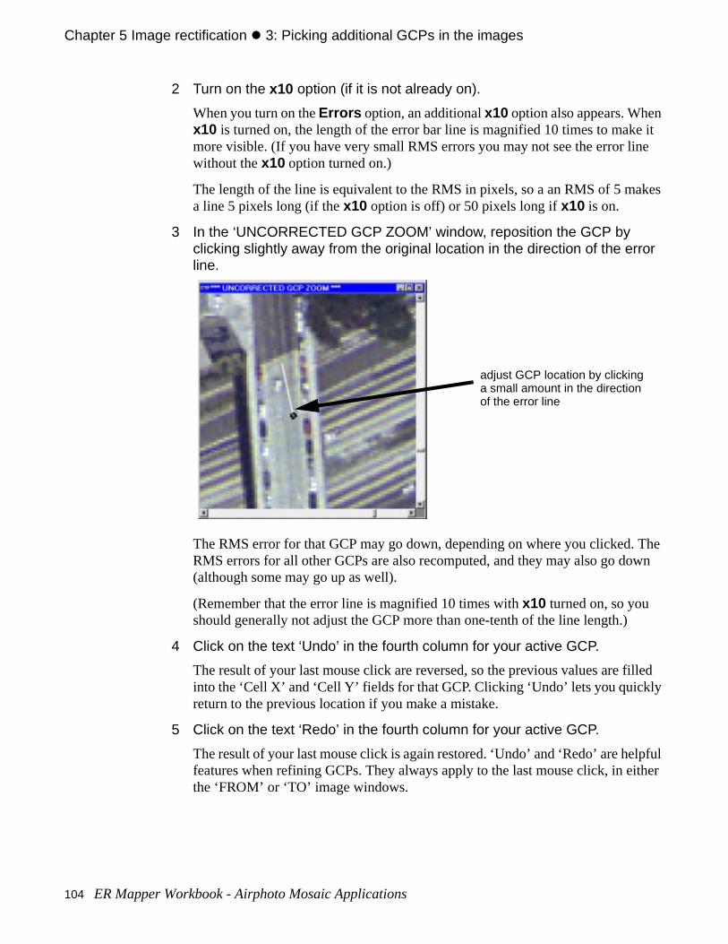
Chapter 5 Image rectification z 3: Picking additional GCPs in the images
e it e
kes
The wn
illed
lpful ither
2 Turn on the x10 option (if it is not already on).
When you turn on the Errors option, an additional x10 option also appears. Whenx10 is turned on, the length of the error bar line is magnified 10 times to makmore visible. (If you have very small RMS errors you may not see the error linwithout the x10 option turned on.)
The length of the line is equivalent to the RMS in pixels, so a an RMS of 5 maa line 5 pixels long (if the x10 option is off) or 50 pixels long if x10 is on.
3 In the ‘UNCORRECTED GCP ZOOM’ window, reposition the GCP by clicking slightly away from the original location in the direction of the error line.
The RMS error for that GCP may go down, depending on where you clicked.RMS errors for all other GCPs are also recomputed, and they may also go do(although some may go up as well).
(Remember that the error line is magnified 10 times with x10 turned on, so you should generally not adjust the GCP more than one-tenth of the line length.)
4 Click on the text ‘Undo’ in the fourth column for your active GCP.
The result of your last mouse click are reversed, so the previous values are finto the ‘Cell X’ and ‘Cell Y’ fields for that GCP. Clicking ‘Undo’ lets you quicklyreturn to the previous location if you make a mistake.
5 Click on the text ‘Redo’ in the fourth column for your active GCP.
The result of your last mouse click is again restored. ‘Undo’ and ‘Redo’ are hefeatures when refining GCPs. They always apply to the last mouse click, in ethe ‘FROM’ or ‘TO’ image windows.
adjust GCP location by clickinga small amount in the directionof the error line
104 ER Mapper Workbook - Airphoto Mosaic Applications
Chapter 5#Image rectification#z 3: Picking additional GCPs in the images
o an es. ou eral
s the ral
ust–ws.
M’e is with
te the
ell
Note: Sometimes an error bar will appear to indicate that you should move a GCP tarea where it clearly does not line up with the chosen feature in the two imagThis can be due to inaccuracies in the reference dataset or other factors, so yshould not rely on the error bar as an absolute indicator. (Use it only as a genguideline.)
Lock a GCP so cannot be edited1 Click on the text ‘Edit’ in the third column for any GCP.
The text changes to ‘No’ and the “X” and number marking it in the image turngreen. This effectively “locks” a GCP so it cannot be edited (that is, clicking inimage windows do not redefine it’s position). This is useful when you have sevevery good GCPs and you to lock them to avoid accidentally changing them.
2 Click on the text ‘No’ in the third column to unlock the GCP.
Enter a label for a GCP1 Select the number text for a GCP under the ‘Name’ column, and type a
short name.
You can give GCPs text labels as well as numbers to help identify them. For example, you might label a GCP for the intersection of the two roads.
Adjust the location or delete GCPs with high errors1 Using the information you learned previously, try to refine the location of
your five highest error GCPs to reduce their RMS error to less than 5.00. The basic procedure is:
• Click on the label under the ‘Name’ column of the GCP you want to adjER Mapper selects the GCP and zooms to it in the two left-hand zoom windo
• Adjust the location of the GCP by clicking in the ‘UNCORRECTED GCP ZOOor ‘CORRECTED GCP ZOOM’ windows to try to reduce the RMS error. (Thera limit to how low an RMS error you can achieve, so don’t be too concernedthis.)
• If you cannot reduce the RMS of a particular GCP, you may choose to dele
GCP altogether by clicking the Delete GCP button. If desired, select a few
more GCPs to account for any you deleted.
At the end, you should have 10 GCPs with RMS errors less than 10.00, and wdistributed throughout the airphoto image.
ER Mapper Workbook - Airphoto Mosaic Applications 105
Chapter 5 Image rectification z 2: Perform the image rectification
ill is
grid uring n.
hat ping
ese
to
Tip: When rectifying images to create a mosaic, it is very important to try to pick GCPs toward the edges of the image where it will overlap with other images. This whelp ensure that features on adjacent images will align well when the mosaiccreated, and minimize offset or shifted features.
View a polynomial grid over the entire airphoto image1 On the GCP Edit dialog, turn on the Grid option.
A green polynomial grid displays over the airphoto image and the three otherimage windows. This grid is a simple “preview” of the way in which the FROM(raw) dataset pixels will be reprojected or translated onto the new coordinateof the TO dataset. The geometry of the raw airphoto image will be changed dthe rectification process so that the grid would be aligned straight up and dow
Typically, the grid should appear as straight, evenly spaced lines for images tcover small geographic areas like this one. If you were to see skewing or warof the grid, this indicates a poor fit of the GCPs in that area of the image.
2 Turn off the Grid option
Save the GCPs to the raw dataset1 Click Save on the GCP Edit dialog. When asked confirm saving the GCPs
to disk, click Yes.
ER Mapper saves the GCPs to the header file of the raw airphoto dataset. Thwill be used to rectify the raw dataset to the UTM map projection coordinatesobtained from the vector roads dataset.
2: Perform the image rectification
Specify output (rectified) image file1 Select the Geocoding Wizard Rectify tab.
2 Click the file chooser button in the Output Info box.
3 From the Directories menu, select the path ending with \examples .
Objectives Learn how to use the ground control points you selected to rectify the image the selected datum and map projection.
106 ER Mapper Workbook - Airphoto Mosaic Applications
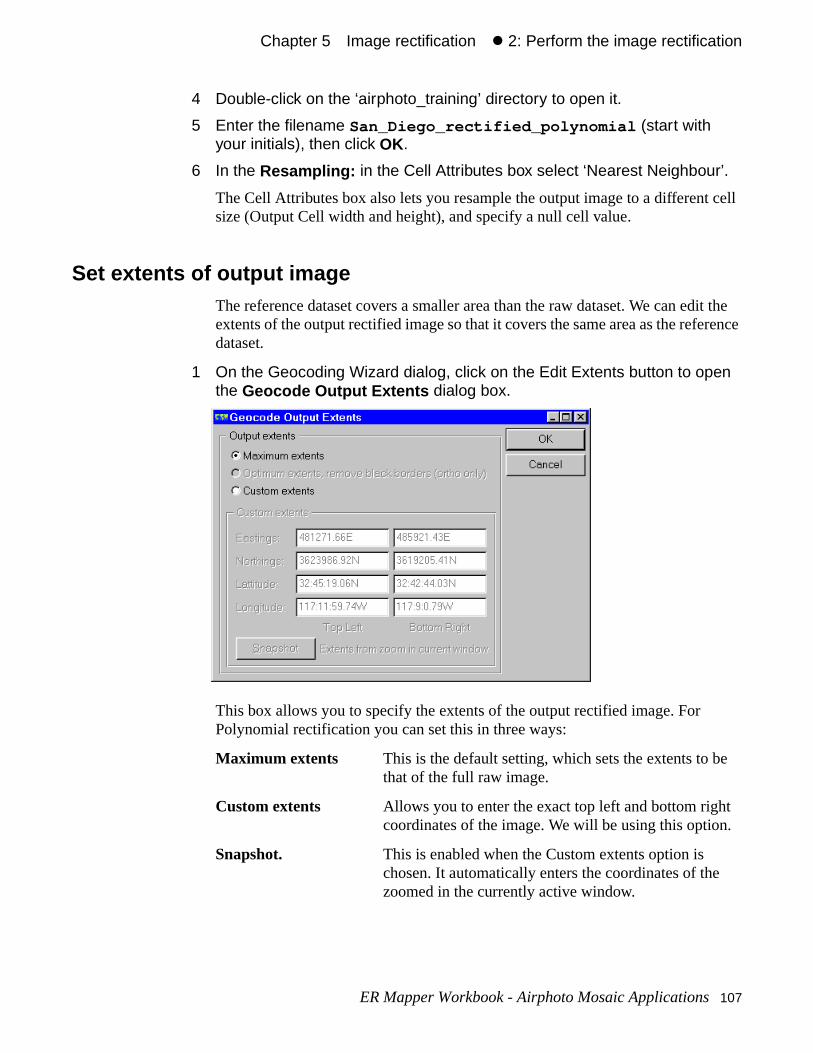
Chapter 5#Image rectification#z 2: Perform the image rectification
cell
it the erence
e
t .
4 Double-click on the ‘airphoto_training’ directory to open it.
5 Enter the filename San_Diego_rectified_polynomial (start with your initials), then click OK.
6 In the Resampling: in the Cell Attributes box select ‘Nearest Neighbour’.
The Cell Attributes box also lets you resample the output image to a differentsize (Output Cell width and height), and specify a null cell value.
Set extents of output imageThe reference dataset covers a smaller area than the raw dataset. We can edextents of the output rectified image so that it covers the same area as the refdataset.
1 On the Geocoding Wizard dialog, click on the Edit Extents button to open the Geocode Output Extents dialog box.
This box allows you to specify the extents of the output rectified image. For Polynomial rectification you can set this in three ways:
Maximum extents This is the default setting, which sets the extents to bthat of the full raw image.
Custom extents Allows you to enter the exact top left and bottom righcoordinates of the image. We will be using this option
Snapshot. This is enabled when the Custom extents option is chosen. It automatically enters the coordinates of thezoomed in the currently active window.
ER Mapper Workbook - Airphoto Mosaic Applications 107
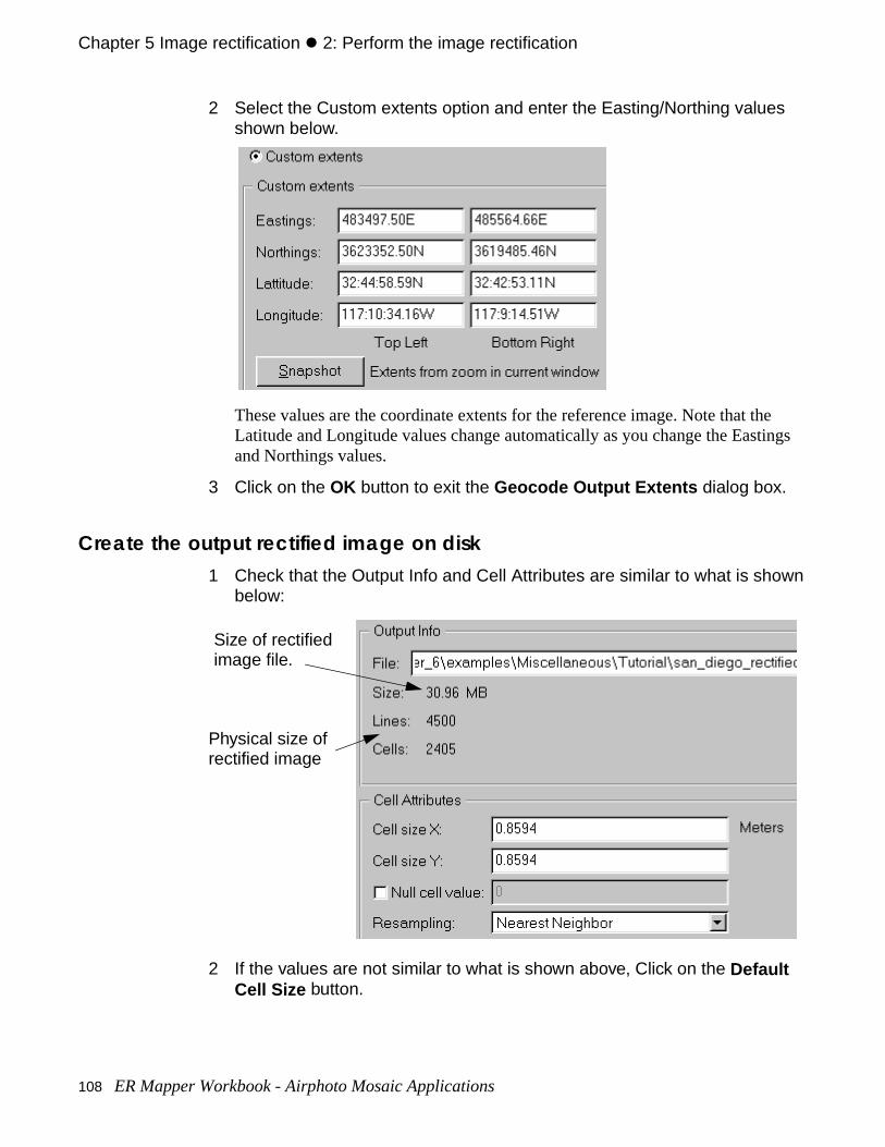
Chapter 5 Image rectification z 2: Perform the image rectification
e ings
2 Select the Custom extents option and enter the Easting/Northing values shown below.
These values are the coordinate extents for the reference image. Note that thLatitude and Longitude values change automatically as you change the Eastand Northings values.
3 Click on the OK button to exit the Geocode Output Extents dialog box.
Create the output rectified image on disk1 Check that the Output Info and Cell Attributes are similar to what is shown
below:
2 If the values are not similar to what is shown above, Click on the Default Cell Size button.
Size of rectifiedimage file.
Physical size ofrectified image
108 ER Mapper Workbook - Airphoto Mosaic Applications
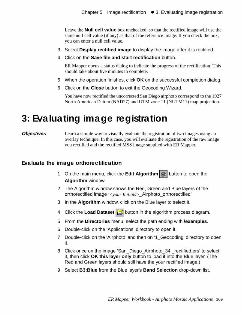
Chapter 5#Image rectification#z 3: Evaluating image registration
he ox,
This
1927 .
n ge
Leave the Null cell value box unchecked, so that the rectified image will use tsame null cell value (if any) as that of the reference image. If you check the byou can enter a null cell value.
3 Select Display rectified image to display the image after it is rectified.
4 Click on the Save file and start rectification button.
ER Mapper opens a status dialog to indicate the progress of the rectification.should take about five minutes to complete.
5 When the operation finishes, click OK on the successful completion dialog.
6 Click on the Close button to exit the Geocoding Wizard.
You have now rectified the uncorrected San Diego airphoto correspond to the North American Datum (NAD27) and UTM zone 11 (NUTM11) map projection
3: Evaluating image registration
Evaluate the image orthorectification
1 On the main menu, click the Edit Algorithm button to open the Algorithm window.
2 The Algorithm window shows the Red, Green and Blue layers of the orthorectified image ‘<your Initials>_Airphoto_orthorectified’
3 In the Algorithm window, click on the Blue layer to select it.
4 Click the Load Dataset button in the algorithm process diagram.
5 From the Directories menu, select the path ending with \examples .
6 Double-click on the ‘Applications’ directory to open it.
7 Double-click on the ‘Airphoto’ and then on ‘1_Geocoding’ directory to open it.
8 Click once on the image ‘San_Diego_Airphoto_34 _rectified.ers’ to select it, then click OK this layer only button to load it into the Blue layer. (The Red and Green layers should still have the your rectified image.)
9 Select B3:Blue from the Blue layer’s Band Selection drop-down list.
Objectives Learn a simple way to visually evaluate the registration of two images using aoverlay technique. In this case, you will evaluate the registration of the raw imayou rectified and the rectified MSS image supplied with ER Mapper.
ER Mapper Workbook - Airphoto Mosaic Applications 109
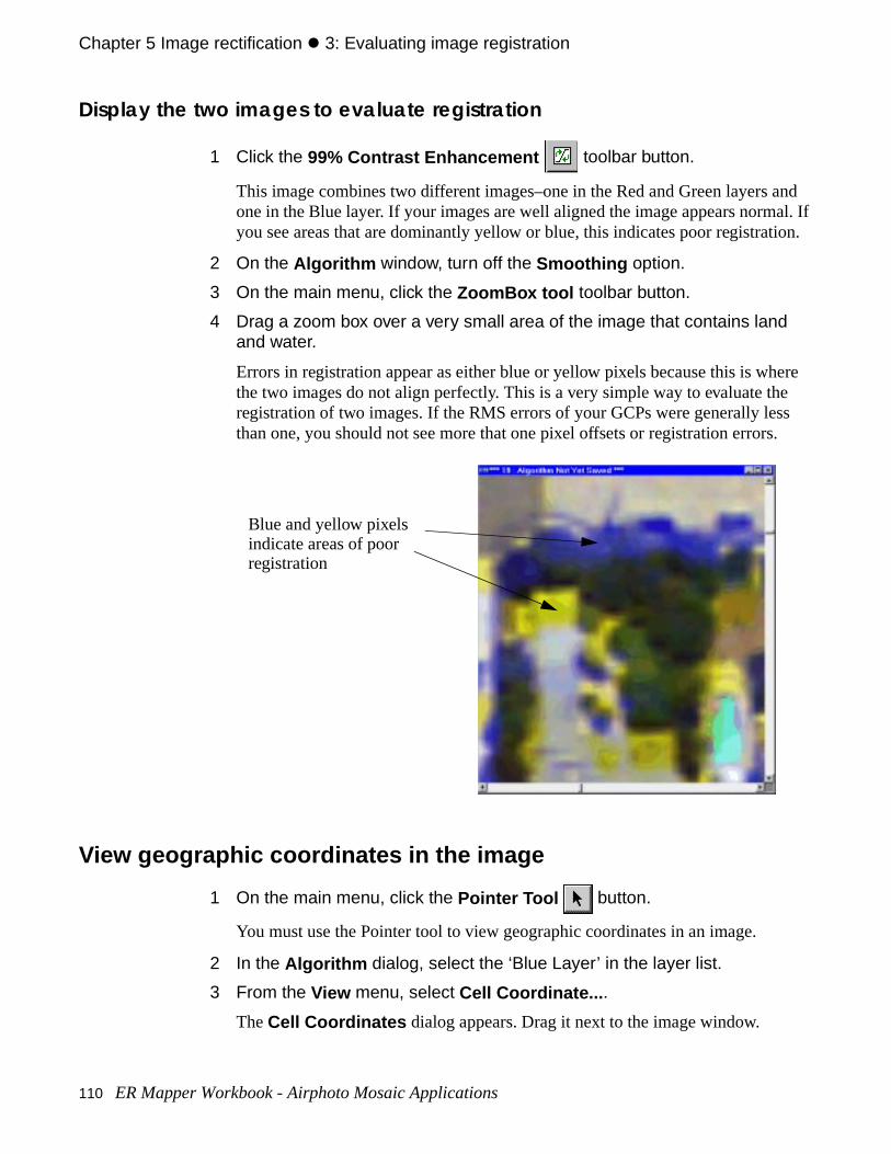
Chapter 5 Image rectification z 3: Evaluating image registration
and al. If ion.
ere e s .
Display the two images to evaluate registration
1 Click the 99% Contrast Enhancement toolbar button.
This image combines two different images–one in the Red and Green layers one in the Blue layer. If your images are well aligned the image appears normyou see areas that are dominantly yellow or blue, this indicates poor registrat
2 On the Algorithm window, turn off the Smoothing option.
3 On the main menu, click the ZoomBox tool toolbar button.
4 Drag a zoom box over a very small area of the image that contains land and water.
Errors in registration appear as either blue or yellow pixels because this is whthe two images do not align perfectly. This is a very simple way to evaluate thregistration of two images. If the RMS errors of your GCPs were generally lesthan one, you should not see more that one pixel offsets or registration errors
View geographic coordinates in the image
1 On the main menu, click the Pointer Tool button.
You must use the Pointer tool to view geographic coordinates in an image.
2 In the Algorithm dialog, select the ‘Blue Layer’ in the layer list.
3 From the View menu, select Cell Coordinate... .
The Cell Coordinates dialog appears. Drag it next to the image window.
Blue and yellow pixelsindicate areas of poorregistration
110 ER Mapper Workbook - Airphoto Mosaic Applications
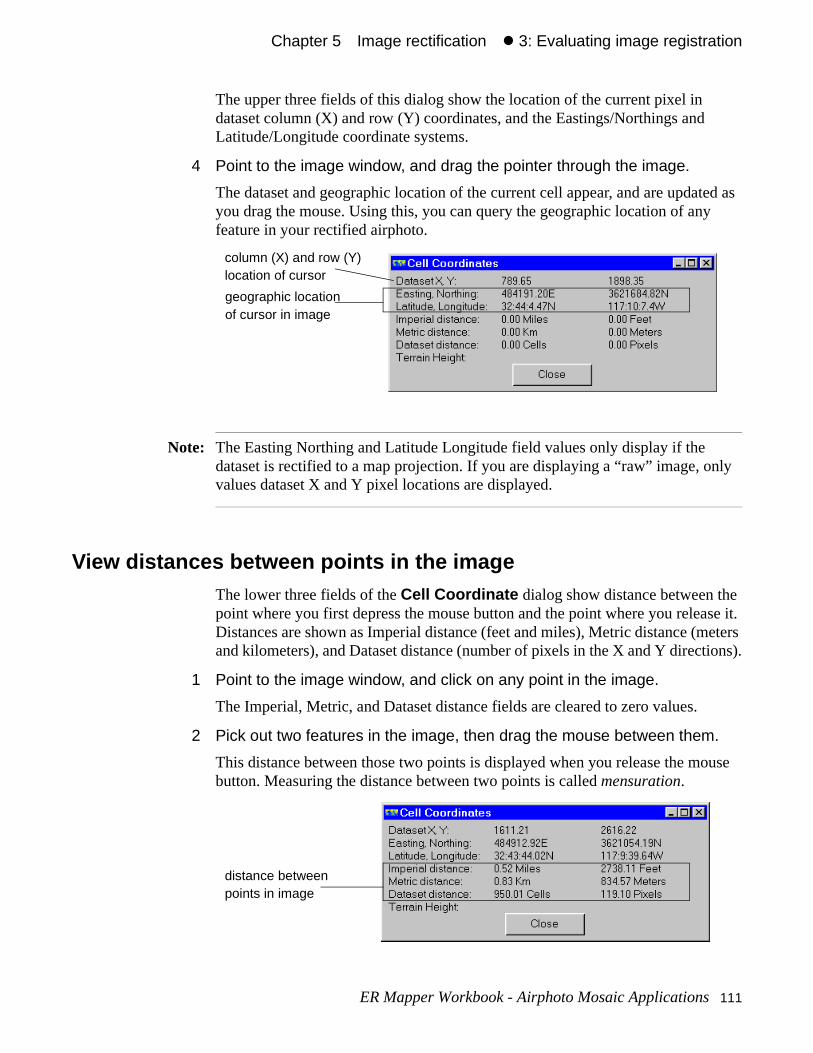
Chapter 5#Image rectification#z 3: Evaluating image registration
ted as y
nly
se it. eters
ions).
ouse
The upper three fields of this dialog show the location of the current pixel in dataset column (X) and row (Y) coordinates, and the Eastings/Northings andLatitude/Longitude coordinate systems.
4 Point to the image window, and drag the pointer through the image.
The dataset and geographic location of the current cell appear, and are updayou drag the mouse. Using this, you can query the geographic location of anfeature in your rectified airphoto.
Note: The Easting Northing and Latitude Longitude field values only display if the dataset is rectified to a map projection. If you are displaying a “raw” image, ovalues dataset X and Y pixel locations are displayed.
View distances between points in the imageThe lower three fields of the Cell Coordinate dialog show distance between thepoint where you first depress the mouse button and the point where you releaDistances are shown as Imperial distance (feet and miles), Metric distance (mand kilometers), and Dataset distance (number of pixels in the X and Y direct
1 Point to the image window, and click on any point in the image.
The Imperial, Metric, and Dataset distance fields are cleared to zero values.
2 Pick out two features in the image, then drag the mouse between them.
This distance between those two points is displayed when you release the mbutton. Measuring the distance between two points is called mensuration.
geographic locationof cursor in image
column (X) and row (Y)location of cursor
distance betweenpoints in image
ER Mapper Workbook - Airphoto Mosaic Applications 111
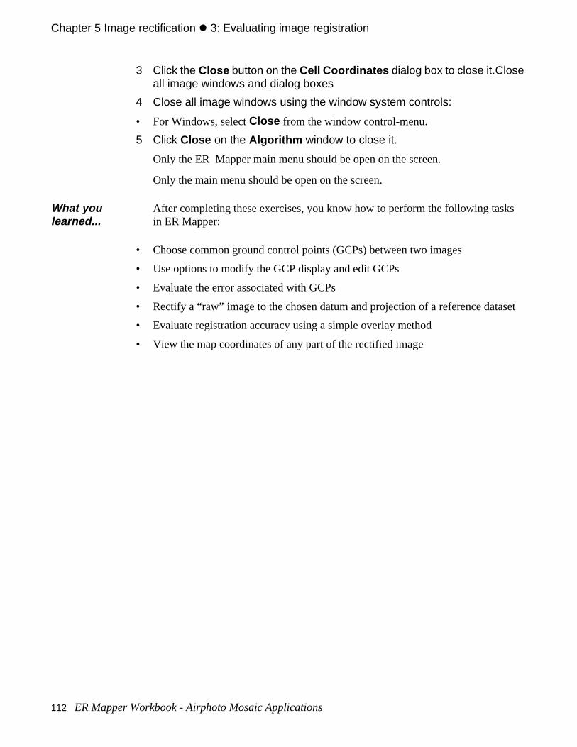
Chapter 5 Image rectification z 3: Evaluating image registration
set
s
3 Click the Close button on the Cell Coordinates dialog box to close it.Close all image windows and dialog boxes
4 Close all image windows using the window system controls:
• For Windows, select Close from the window control-menu.
5 Click Close on the Algorithm window to close it.
Only the ER Mapper main menu should be open on the screen.
Only the main menu should be open on the screen.
• Choose common ground control points (GCPs) between two images
• Use options to modify the GCP display and edit GCPs
• Evaluate the error associated with GCPs
• Rectify a “raw” image to the chosen datum and projection of a reference data
• Evaluate registration accuracy using a simple overlay method
• View the map coordinates of any part of the rectified image
What you learned...
After completing these exercises, you know how to perform the following taskin ER Mapper:
112 ER Mapper Workbook - Airphoto Mosaic Applications
te
use
red in
d by the
t
6
Imageorthorectification
This chapter explains how to use the ER Mapper Geocoding Wizard to geometrically correct raw image data and orthorectify it to real world coordinasystems and map projections.
About orthorectificationOrthorectification is more accurate than Linear or Polynomial rectification becait corrects local and global distortions in an image by adjusting for camera characteristics, platform positions and terrain details.
The camera characteristics, derived from a camera calibration report, are stoa camera file for use by the Geocoding Wizard.
The terrain details are supplied in the form of a DEM. If the terrain is relativelyflat, you can use an average height value.
In the case of Advanced Orthorectification, the platform position is determineexterior orientation values which describe the exact position of the aircraft at time the image was taken, and how this relates to the image. The following parameters are specified:
Attitude omega The tilt angle (roll) of the aircraft; i.e. the rotation abouthe X axis (direction of travel).
ER Mapper Workbook - Land Information 113
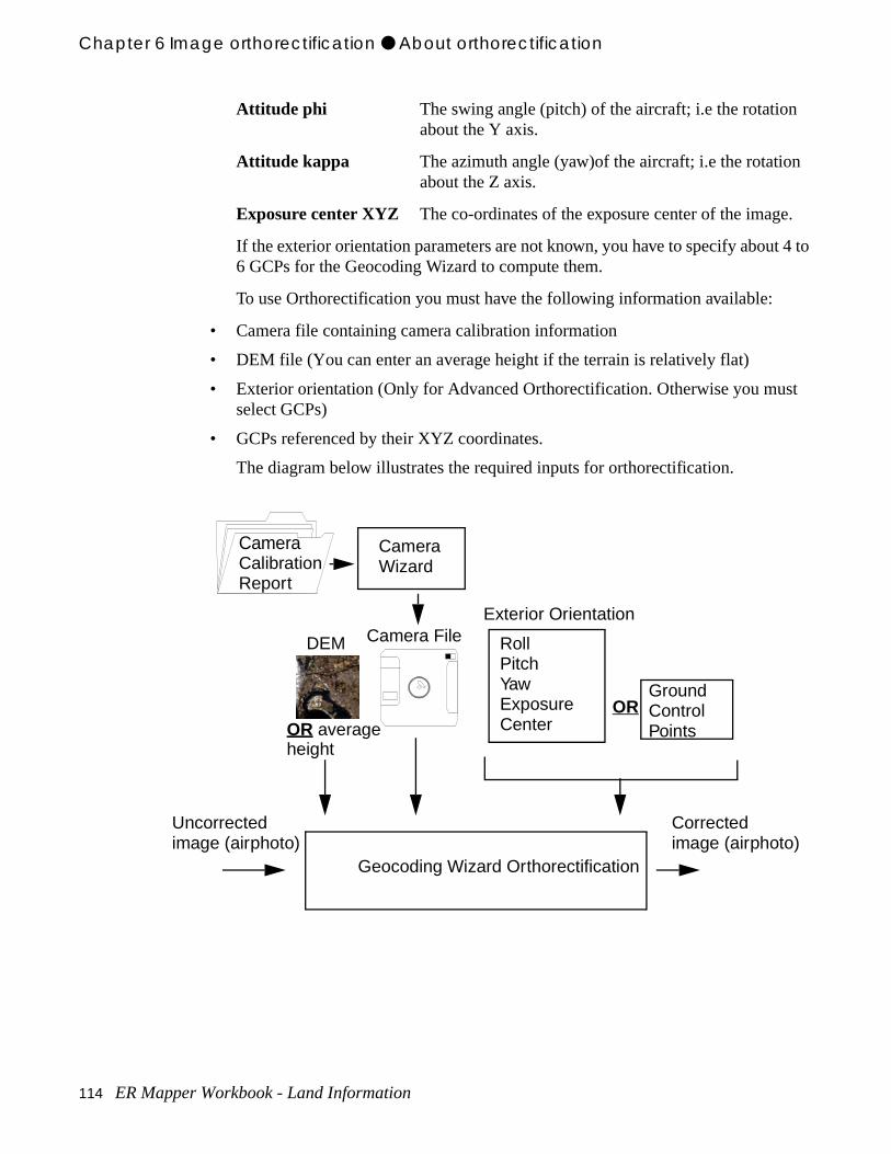
Chapter 6 Image orthorectification ● About orthorectification
.
t 4 to
t
Attitude phi The swing angle (pitch) of the aircraft; i.e the rotationabout the Y axis.
Attitude kappa The azimuth angle (yaw)of the aircraft; i.e the rotationabout the Z axis.
Exposure center XYZ The co-ordinates of the exposure center of the image
If the exterior orientation parameters are not known, you have to specify abou6 GCPs for the Geocoding Wizard to compute them.
To use Orthorectification you must have the following information available:
• Camera file containing camera calibration information
• DEM file (You can enter an average height if the terrain is relatively flat)
• Exterior orientation (Only for Advanced Orthorectification. Otherwise you musselect GCPs)
• GCPs referenced by their XYZ coordinates.
The diagram below illustrates the required inputs for orthorectification.
Geocoding Wizard Orthorectification
CameraWizard
Camera FileDEM RollPitchYawExposureCenter
Exterior Orientation
Ground ControlPoints
OR
Uncorrectedimage (airphoto)
Correctedimage (airphoto)
OR averageheight
CameraCalibrationReport
114 ER Mapper Workbook - Land Information
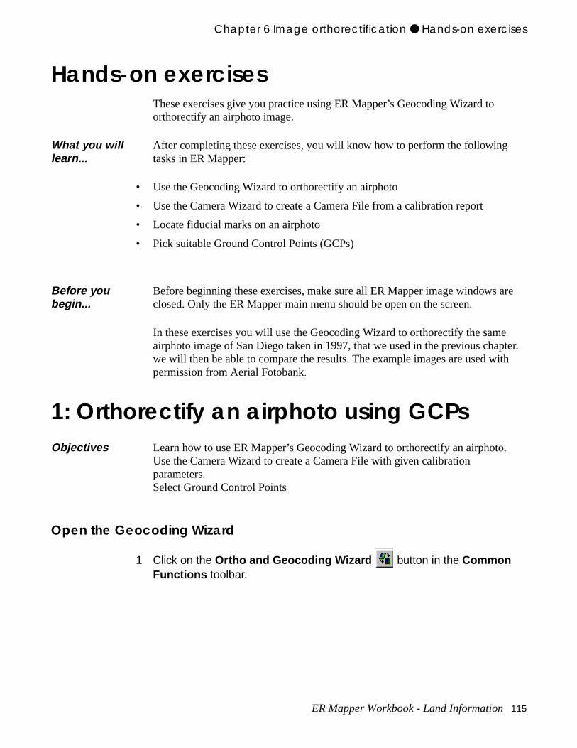
Chapter 6 Image orthorectification ● Hands-on exercises
e pter. ith
are
Hands-on exercisesThese exercises give you practice using ER Mapper’s Geocoding Wizard to orthorectify an airphoto image.
• Use the Geocoding Wizard to orthorectify an airphoto
• Use the Camera Wizard to create a Camera File from a calibration report
• Locate fiducial marks on an airphoto
• Pick suitable Ground Control Points (GCPs)
In these exercises you will use the Geocoding Wizard to orthorectify the samairphoto image of San Diego taken in 1997, that we used in the previous chawe will then be able to compare the results. The example images are used wpermission from Aerial Fotobank.
1: Orthorectify an airphoto using GCPs
Open the Geocoding Wizard
1 Click on the Ortho and Geocoding Wizard button in the Common Functions toolbar.
What you will learn...
After completing these exercises, you will know how to perform the following tasks in ER Mapper:
Before you begin...
Before beginning these exercises, make sure all ER Mapper image windows closed. Only the ER Mapper main menu should be open on the screen.
Objectives Learn how to use ER Mapper’s Geocoding Wizard to orthorectify an airphoto.Use the Camera Wizard to create a Camera File with given calibration parameters.Select Ground Control Points
ER Mapper Workbook - Land Information 115
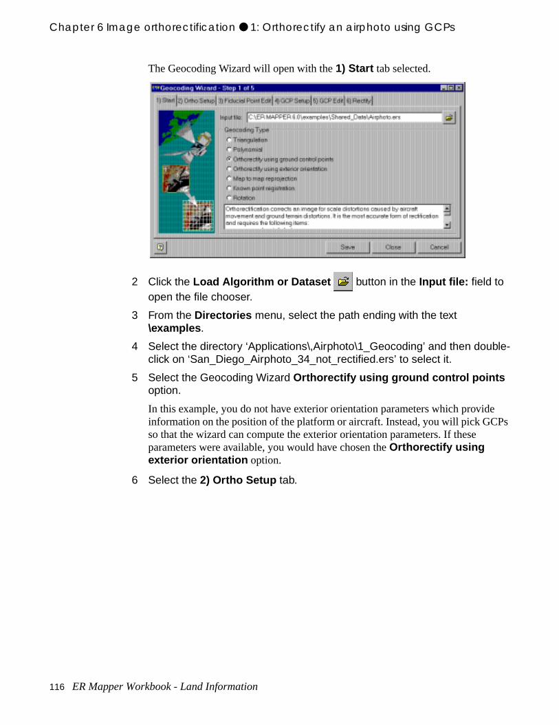
Chapter 6 Image orthorectification ● 1: Orthorectify an airphoto using GCPs
e Ps
The Geocoding Wizard will open with the 1) Start tab selected.
2 Click the Load Algorithm or Dataset button in the Input file: field to open the file chooser.
3 From the Directories menu, select the path ending with the text \examples .
4 Select the directory ‘Applications\,Airphoto\1_Geocoding’ and then double-click on ‘San_Diego_Airphoto_34_not_rectified.ers’ to select it.
5 Select the Geocoding Wizard Orthorectify using ground control points option.
In this example, you do not have exterior orientation parameters which providinformation on the position of the platform or aircraft. Instead, you will pick GCso that the wizard can compute the exterior orientation parameters. If these parameters were available, you would have chosen the Orthorectify using exterior orientation option.
6 Select the 2) Ortho Setup tab.
116 ER Mapper Workbook - Land Information
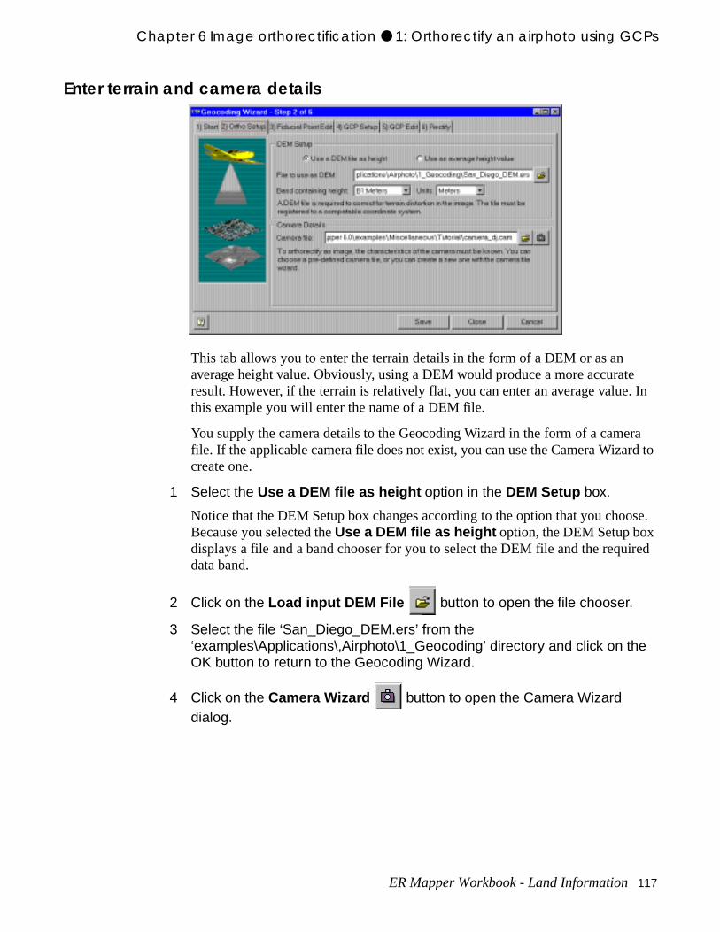
Chapter 6 Image orthorectification ● 1: Orthorectify an airphoto using GCPs
te . In
ra rd to
ose.
ired
Enter terrain and camera details
This tab allows you to enter the terrain details in the form of a DEM or as an average height value. Obviously, using a DEM would produce a more accuraresult. However, if the terrain is relatively flat, you can enter an average valuethis example you will enter the name of a DEM file.
You supply the camera details to the Geocoding Wizard in the form of a camefile. If the applicable camera file does not exist, you can use the Camera Wizacreate one.
1 Select the Use a DEM file as height option in the DEM Setup box.
Notice that the DEM Setup box changes according to the option that you choBecause you selected the Use a DEM file as height option, the DEM Setup box displays a file and a band chooser for you to select the DEM file and the requdata band.
2 Click on the Load input DEM File button to open the file chooser.
3 Select the file ‘San_Diego_DEM.ers’ from the ‘examples\Applications\,Airphoto\1_Geocoding’ directory and click on the OK button to return to the Geocoding Wizard.
4 Click on the Camera Wizard button to open the Camera Wizard dialog.
ER Mapper Workbook - Land Information 117
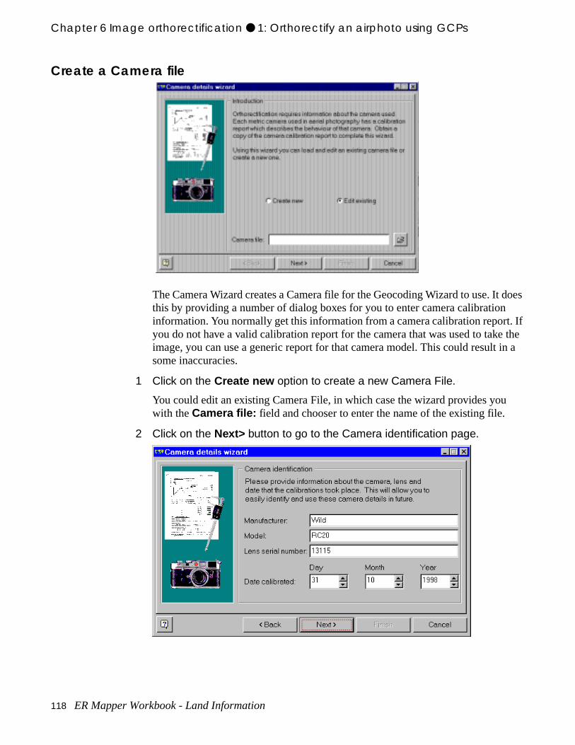
Chapter 6 Image orthorectification ● 1: Orthorectify an airphoto using GCPs
does
t. If e the in a
Create a Camera file
The Camera Wizard creates a Camera file for the Geocoding Wizard to use. Itthis by providing a number of dialog boxes for you to enter camera calibrationinformation. You normally get this information from a camera calibration reporyou do not have a valid calibration report for the camera that was used to takimage, you can use a generic report for that camera model. This could resultsome inaccuracies.
1 Click on the Create new option to create a new Camera File.
You could edit an existing Camera File, in which case the wizard provides youwith the Camera file: field and chooser to enter the name of the existing file.
2 Click on the Next> button to go to the Camera identification page.
118 ER Mapper Workbook - Land Information
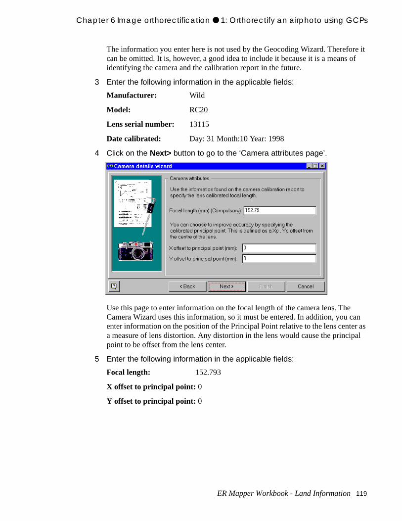
Chapter 6 Image orthorectification ● 1: Orthorectify an airphoto using GCPs
re it of
can er as pal
The information you enter here is not used by the Geocoding Wizard. Therefocan be omitted. It is, however, a good idea to include it because it is a meansidentifying the camera and the calibration report in the future.
3 Enter the following information in the applicable fields:
Manufacturer: Wild
Model: RC20
Lens serial number: 13115
Date calibrated: Day: 31 Month:10 Year: 1998
4 Click on the Next> button to go to the ‘Camera attributes page’.
Use this page to enter information on the focal length of the camera lens. TheCamera Wizard uses this information, so it must be entered. In addition, you enter information on the position of the Principal Point relative to the lens centa measure of lens distortion. Any distortion in the lens would cause the principoint to be offset from the lens center.
5 Enter the following information in the applicable fields:
Focal length: 152.793
X offset to principal point: 0
Y offset to principal point: 0
ER Mapper Workbook - Land Information 119
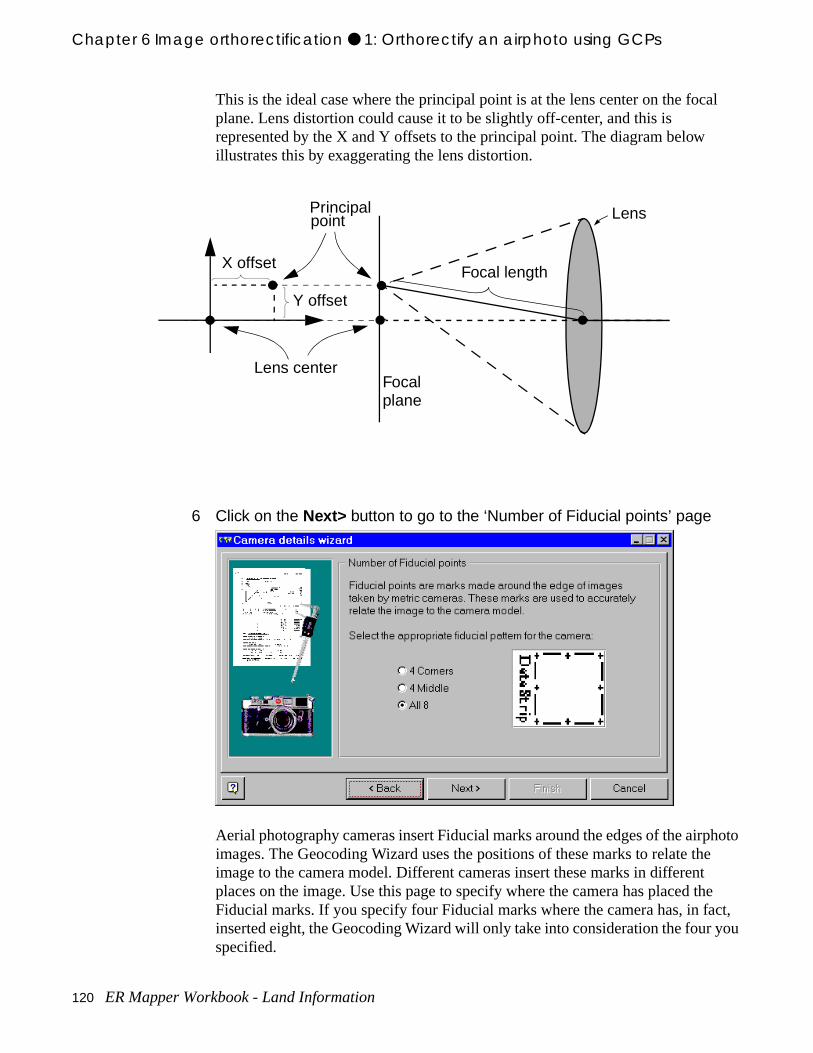
Chapter 6 Image orthorectification ● 1: Orthorectify an airphoto using GCPs
al
photo e the ct, you
This is the ideal case where the principal point is at the lens center on the focplane. Lens distortion could cause it to be slightly off-center, and this is represented by the X and Y offsets to the principal point. The diagram below illustrates this by exaggerating the lens distortion.
6 Click on the Next> button to go to the ‘Number of Fiducial points’ page
Aerial photography cameras insert Fiducial marks around the edges of the airimages. The Geocoding Wizard uses the positions of these marks to relate thimage to the camera model. Different cameras insert these marks in differentplaces on the image. Use this page to specify where the camera has placed Fiducial marks. If you specify four Fiducial marks where the camera has, in fainserted eight, the Geocoding Wizard will only take into consideration the four specified.
Principalpoint
Focal length
Lens
Y offset
X offset
Lens centerFocalplane
120 ER Mapper Workbook - Land Information
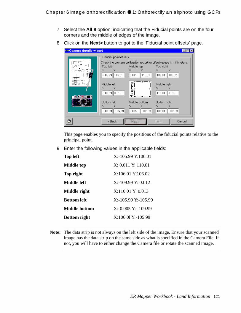
Chapter 6 Image orthorectification ● 1: Orthorectify an airphoto using GCPs
the
nned File. If e.
7 Select the All 8 option; indicating that the Fiducial points are on the four corners and the middle of edges of the image.
8 Click on the Next> button to got to the ‘Fiducial point offsets’ page.
This page enables you to specify the positions of the fiducial points relative toprincipal point.
9 Enter the following values in the applicable fields:
Top left X:-105.99 Y:106.01
Middle top X: 0.011 Y: 110.01
Top right X:106.01 Y:106.02
Middle left X:-109.99 Y: 0.012
Middle right X:110.01 Y: 0.013
Bottom left X:-105.99 Y:-105.99
Middle bottom X:-0.005 Y: -109.99
Bottom right X:106.0l Y:-105.99
Note: The data strip is not always on the left side of the image. Ensure that your scaimage has the data strip on the same side as what is specified in the Camera not, you will have to either change the Camera file or rotate the scanned imag
ER Mapper Workbook - Land Information 121
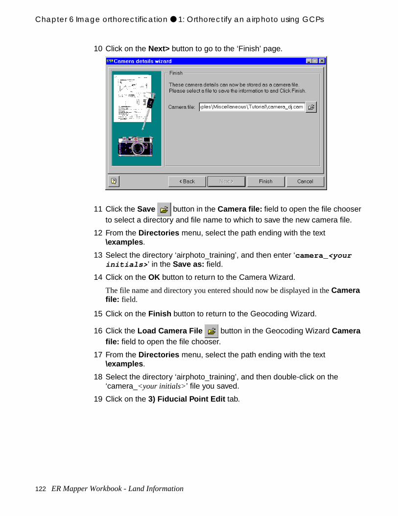
Chapter 6 Image orthorectification ● 1: Orthorectify an airphoto using GCPs
10 Click on the Next> button to go to the ‘Finish’ page.
11 Click the Save button in the Camera file: field to open the file chooser to select a directory and file name to which to save the new camera file.
12 From the Directories menu, select the path ending with the text \examples .
13 Select the directory ‘airphoto_training’, and then enter ‘camera_ <your initials> ’ in the Save as: field.
14 Click on the OK button to return to the Camera Wizard.
The file name and directory you entered should now be displayed in the Camera file: field.
15 Click on the Finish button to return to the Geocoding Wizard.
16 Click the Load Camera File button in the Geocoding Wizard Camera file: field to open the file chooser.
17 From the Directories menu, select the path ending with the text \examples .
18 Select the directory ‘airphoto_training’, and then double-click on the ‘camera_<your initials>’ file you saved.
19 Click on the 3) Fiducial Point Edit tab.
122 ER Mapper Workbook - Land Information
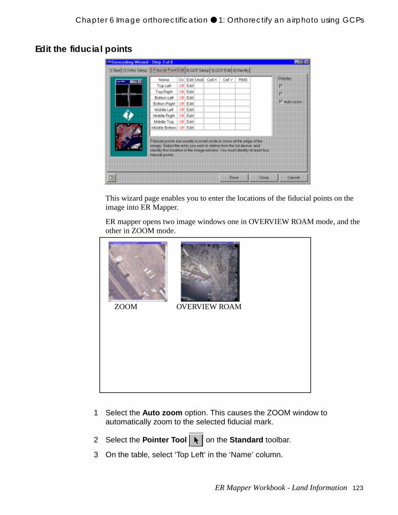
Chapter 6 Image orthorectification ● 1: Orthorectify an airphoto using GCPs
he
the
Edit the fiducial points
This wizard page enables you to enter the locations of the fiducial points on timage into ER Mapper.
ER mapper opens two image windows one in OVERVIEW ROAM mode, and other in ZOOM mode.
1 Select the Auto zoom option. This causes the ZOOM window to automatically zoom to the selected fiducial mark.
2 Select the Pointer Tool on the Standard toolbar.
3 On the table, select ‘Top Left’ in the ‘Name’ column.
ZOOM OVERVIEW ROAM
ER Mapper Workbook - Land Information 123
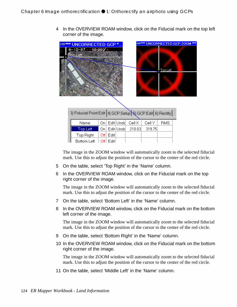
Chapter 6 Image orthorectification ● 1: Orthorectify an airphoto using GCPs
ial le.
ial le.
ial le.
ial le.
4 In the OVERVIEW ROAM window, click on the Fiducial mark on the top left corner of the image.
The image in the ZOOM window will automatically zoom to the selected fiducmark. Use this to adjust the position of the cursor to the center of the red circ
5 On the table, select ‘Top Right’ in the ‘Name’ column.
6 In the OVERVIEW ROAM window, click on the Fiducial mark on the top right corner of the image.
The image in the ZOOM window will automatically zoom to the selected fiducmark. Use this to adjust the position of the cursor to the center of the red circ
7 On the table, select ‘Bottom Left’ in the ‘Name’ column.
8 In the OVERVIEW ROAM window, click on the Fiducial mark on the bottom left corner of the image.
The image in the ZOOM window will automatically zoom to the selected fiducmark. Use this to adjust the position of the cursor to the center of the red circ
9 On the table, select ‘Bottom Right’ in the ‘Name’ column.
10 In the OVERVIEW ROAM window, click on the Fiducial mark on the bottom right corner of the image.
The image in the ZOOM window will automatically zoom to the selected fiducmark. Use this to adjust the position of the cursor to the center of the red circ
11 On the table, select ‘Middle Left’ in the ‘Name’ column.
124 ER Mapper Workbook - Land Information
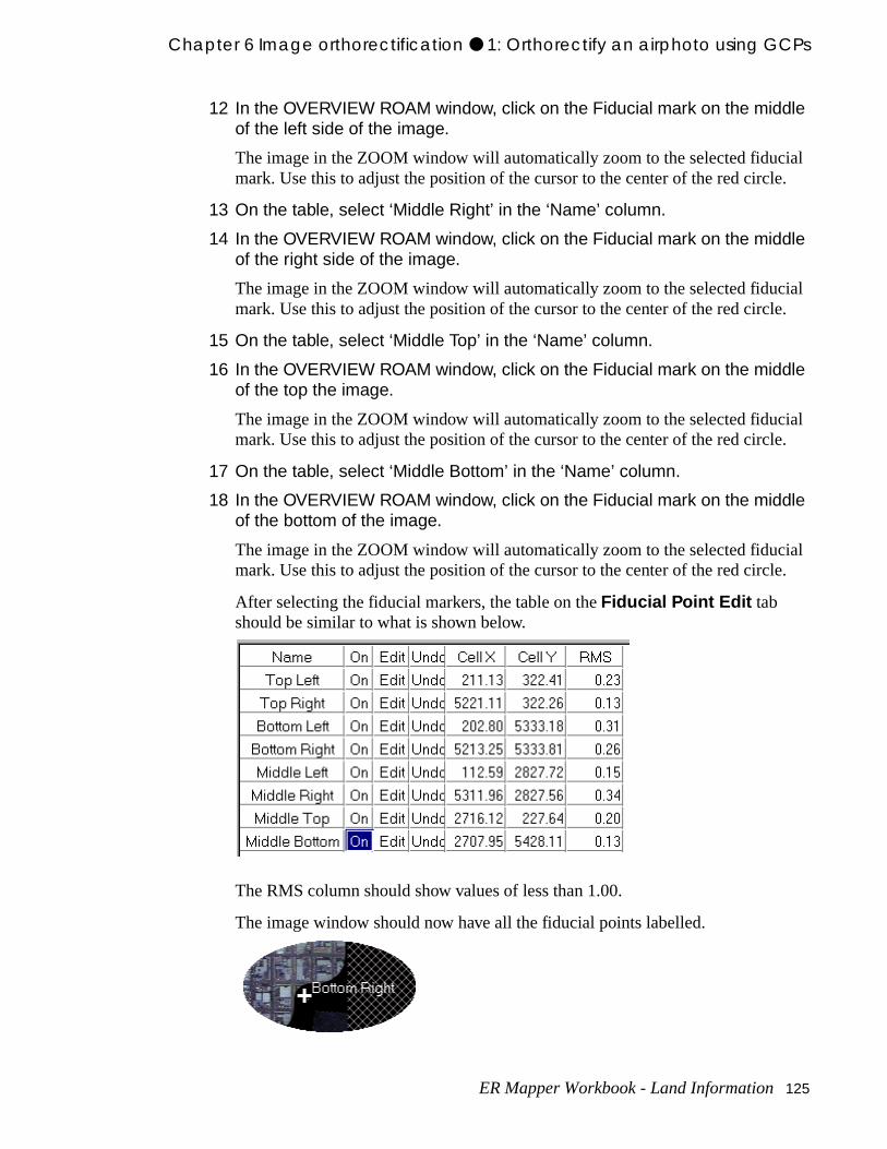
Chapter 6 Image orthorectification ● 1: Orthorectify an airphoto using GCPs
ial le.
ial le.
ial le.
ial le.
12 In the OVERVIEW ROAM window, click on the Fiducial mark on the middle of the left side of the image.
The image in the ZOOM window will automatically zoom to the selected fiducmark. Use this to adjust the position of the cursor to the center of the red circ
13 On the table, select ‘Middle Right’ in the ‘Name’ column.
14 In the OVERVIEW ROAM window, click on the Fiducial mark on the middle of the right side of the image.
The image in the ZOOM window will automatically zoom to the selected fiducmark. Use this to adjust the position of the cursor to the center of the red circ
15 On the table, select ‘Middle Top’ in the ‘Name’ column.
16 In the OVERVIEW ROAM window, click on the Fiducial mark on the middle of the top the image.
The image in the ZOOM window will automatically zoom to the selected fiducmark. Use this to adjust the position of the cursor to the center of the red circ
17 On the table, select ‘Middle Bottom’ in the ‘Name’ column.
18 In the OVERVIEW ROAM window, click on the Fiducial mark on the middle of the bottom of the image.
The image in the ZOOM window will automatically zoom to the selected fiducmark. Use this to adjust the position of the cursor to the center of the red circ
After selecting the fiducial markers, the table on the Fiducial Point Edit tab should be similar to what is shown below.
The RMS column should show values of less than 1.00.
The image window should now have all the fiducial points labelled.
ER Mapper Workbook - Land Information 125
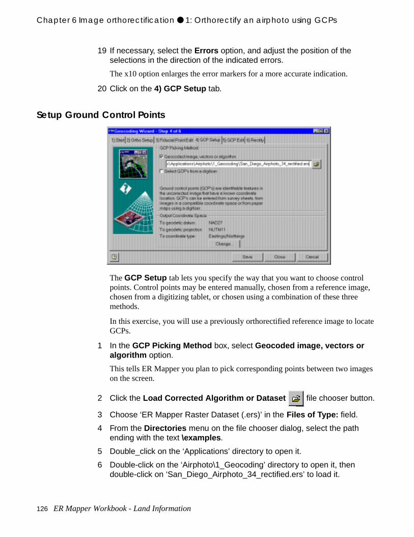
Chapter 6 Image orthorectification ● 1: Orthorectify an airphoto using GCPs
ge,
ate
ges
19 If necessary, select the Errors option, and adjust the position of the selections in the direction of the indicated errors.
The x10 option enlarges the error markers for a more accurate indication.
20 Click on the 4) GCP Setup tab.
Setup Ground Control Points
The GCP Setup tab lets you specify the way that you want to choose control points. Control points may be entered manually, chosen from a reference imachosen from a digitizing tablet, or chosen using a combination of these three methods.
In this exercise, you will use a previously orthorectified reference image to locGCPs.
1 In the GCP Picking Method box, select Geocoded image, vectors or algorithm option.
This tells ER Mapper you plan to pick corresponding points between two imaon the screen.
2 Click the Load Corrected Algorithm or Dataset file chooser button.
3 Choose ‘ER Mapper Raster Dataset (.ers)’ in the Files of Type: field.
4 From the Directories menu on the file chooser dialog, select the path ending with the text \examples .
5 Double_click on the ‘Applications’ directory to open it.
6 Double-click on the ‘Airphoto\1_Geocoding’ directory to open it, then double-click on ‘San_Diego_Airphoto_34_rectified.ers’ to load it.
126 ER Mapper Workbook - Land Information
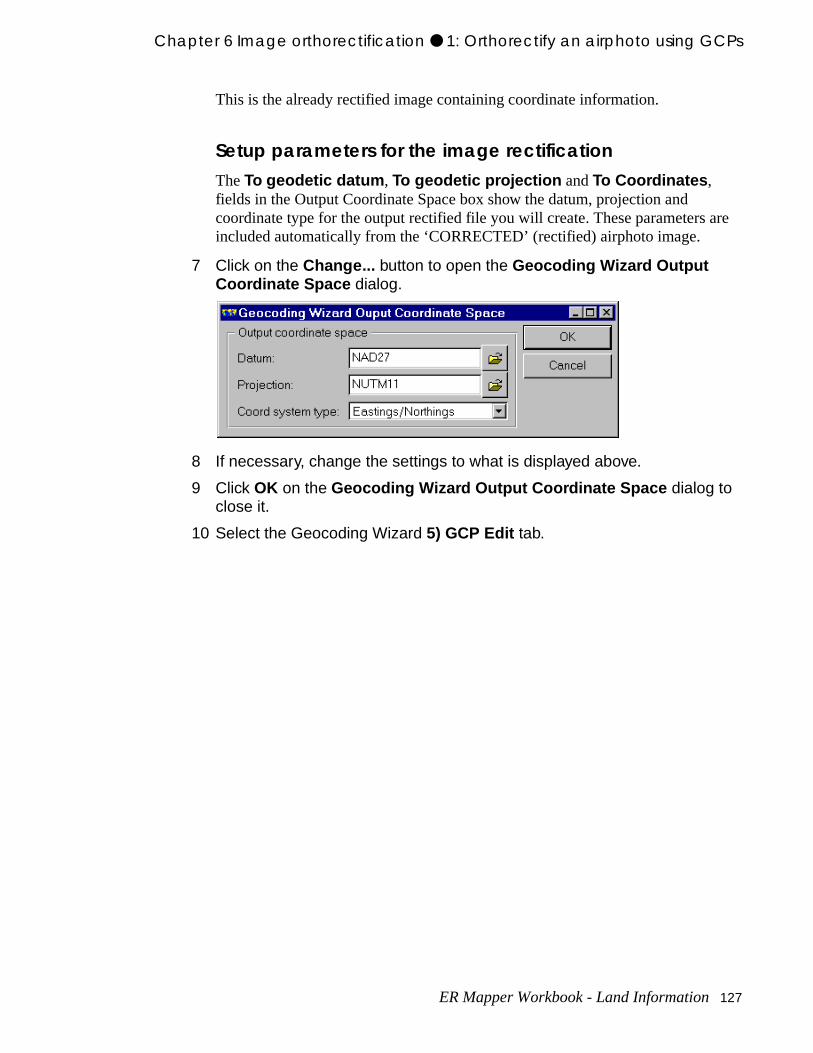
Chapter 6 Image orthorectification ● 1: Orthorectify an airphoto using GCPs
are
This is the already rectified image containing coordinate information.
Setup parameters for the image rectificationThe To geodetic datum , To geodetic projection and To Coordinates , fields in the Output Coordinate Space box show the datum, projection and coordinate type for the output rectified file you will create. These parameters included automatically from the ‘CORRECTED’ (rectified) airphoto image.
7 Click on the Change... button to open the Geocoding Wizard Output Coordinate Space dialog.
8 If necessary, change the settings to what is displayed above.
9 Click OK on the Geocoding Wizard Output Coordinate Space dialog to close it.
10 Select the Geocoding Wizard 5) GCP Edit tab.
ER Mapper Workbook - Land Information 127
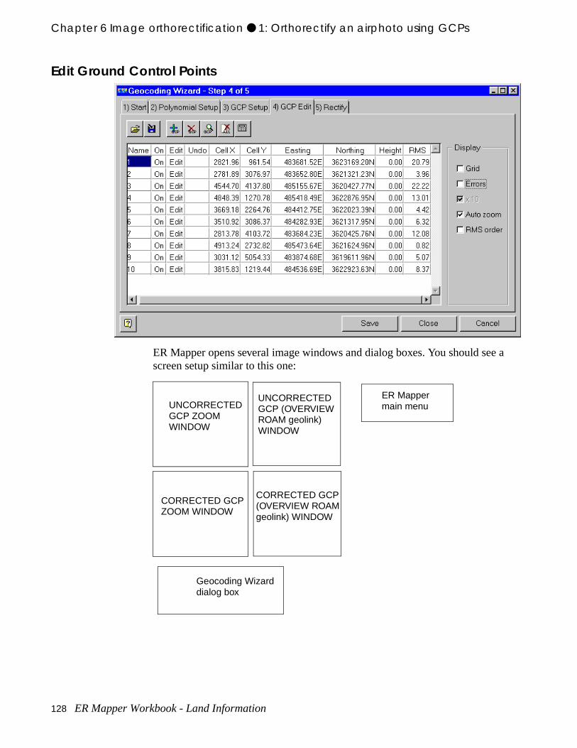
Chapter 6 Image orthorectification ● 1: Orthorectify an airphoto using GCPs
a
Edit Ground Control Points
ER Mapper opens several image windows and dialog boxes. You should see screen setup similar to this one:
ER Mappermain menu
Geocoding Wizarddialog box
UNCORRECTEDGCP ZOOMWINDOW
CORRECTED GCPZOOM WINDOW
UNCORRECTEDGCP (OVERVIEWROAM geolink)WINDOW
CORRECTED GCP(OVERVIEW ROAMgeolink) WINDOW
128 ER Mapper Workbook - Land Information
Chapter 6 Image orthorectification ● 1: Orthorectify an airphoto using GCPs
s
ectify
ove
e
Note: If your system does not position the windows automatically, rearrange them ashown above before proceeding.
The GCP Edit box should already have the GCPs you picked in the previous exercise. To save time we can use these existing GCPs and go straight to “Rthe image” on page 131. Orthorectification only requires 4 to 6 GCPs, so youmight want to delete those that show a high RMS error value.
Pick a GCP in the upper-left part of both images
Note: Make sure the main ER Mapper menu is not hidden by the image windows–mit slightly if needed so you can easily access the toolbars.
1 On the Geocoding Wizard GCP Edit tab, select Auto zoom .
The ZOOM windows will now automatically zoom into the point selected in thcorresponding OVERVIEW ROAM windows.
2 Click on a well defined feature in the ‘UNCORRECTED GCP (OVERVIEW ROAM geolink)’ window to select it.
The ‘UNCORRECTED GCP ZOOM’ window will zoom ito the selected point
3 Click once in the ‘CORRECTED GCP (OVERVIEW ROAM geolink)’ window to activate it, then click on the same feature to select it as a GCP.
The ‘CORRECTED GCP ZOOM’ window will zoom ito the selected point
4 Use the two ZOOM windows to adjust the positions of the GCP.
You have now picked a GCP in the image.
Pick a second GCP in the lower-left of both images
5 On the Geocoding Wizard Edit GCP dialog, click the Add new GCP
button.
6 Click on a well defined feature in the ‘UNCORRECTED GCP (OVERVIEW ROAM geolink)’ window to select it.
The ‘UNCORRECTED GCP ZOOM’ window will zoom into the selected point
7 Click once in the ‘CORRECTED GCP (OVERVIEW ROAM geolink)’ window to activate it, then click on the same feature to select it as a GCP.
The ‘CORRECTED GCP ZOOM’ window will zoom ito the selected point
ER Mapper Workbook - Land Information 129
Chapter 6 Image orthorectification ● 1: Orthorectify an airphoto using GCPs
tion
ing
sing
s the eral
8 Use the two ZOOM windows to adjust the positions of the GCP.
You have now picked a second GCP in the image.
9 Following the above steps, pick another four GCPs near the upper-right, lower-right and middle of the images.
The more GCPs you pick the lower the possibility of errors. For orthorectificayou need at least six.
Try some other features on the Geocoding Wizard GCP Edit dialog1 In the Geocoding Wizard GCP Edit dialog, click on any GCP number under
the ‘Name’ column.
ER Mapper moves the crosshairs to highlight that point in all the ‘OVERVIEWROAM’ and ‘ZOOM’ windows.
2 Turn off the Auto Zoom option at the bottom.
3 Click on any GCP number under the ‘Name’ column.
ER Mapper moves the crosshairs to highlight that point in the ‘OVERVIEW ROAM’ windows, but not the ‘ZOOM’ windows.
4 Click on the Zoom to current GCP button.
ER Mapper zooms into the selected GCP in the “ZOOM’ windows.
5 Select the number text for a GCP under the ‘Name’ column, and type a short name.
You can give GCPs text labels as well as numbers to help identify them.
6 Click on the text ‘On’ in the second column for any GCP.
The text changes to ‘Off’ and all the RMS errors are recomputed without includthat GCP. (This is an easy way to see how the positional error of any GCP influences the RMS of the others. For example, turning off a GCP with a largeRMS often reduces the RMS of the others.) This can be important when choowhich GCPs will be used for the final image rectification.
7 Turn off other GCPs to see the effect, but turn all on again when finished.
8 Click on the text ‘Edit’ in the third column for any GCP.
The text changes to ‘No’ and the “X” and number marking it in the image turngreen. This effectively “locks” a GCP so it cannot be edited (that is, clicking inimage windows do not redefine it’s position). This is useful when you have sevvery good GCPs and you to lock them to avoid accidentally changing them.
9 Turn on the Errors option.
130 ER Mapper Workbook - Land Information
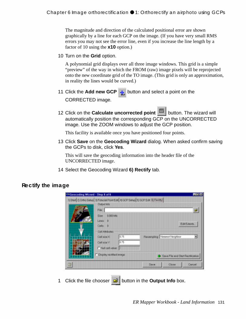
Chapter 6 Image orthorectification ● 1: Orthorectify an airphoto using GCPs
tion,
The magnitude and direction of the calculated positional error are shown graphically by a line for each GCP on the image. (If you have very small RMSerrors you may not see the error line, even if you increase the line length by afactor of 10 using the x10 option.)
10 Turn on the Grid option.
A polynomial grid displays over all three image windows. This grid is a simple“preview” of the way in which the FROM (raw) image pixels will be reprojectedonto the new coordinate grid of the TO image. (This grid is only an approximain reality the lines would be curved.)
11 Click the Add new GCP button and select a point on the
CORRECTED image.
12 Click on the Calculate uncorrected point button. The wizard will automatically position the corresponding GCP on the UNCORRECTED image. Use the ZOOM windows to adjust the GCP position.
This facility is available once you have positioned four points.
13 Click Save on the Geocoding Wizard dialog. When asked confirm saving the GCPs to disk, click Yes.
This will save the geocoding information into the header file of the UNCORRECTED image.
14 Select the Geocoding Wizard 6) Rectify tab.
Rectify the image
1 Click the file chooser button in the Output Info box.
ER Mapper Workbook - Land Information 131
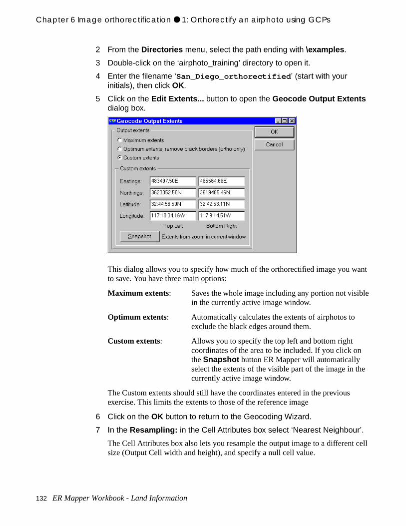
Chapter 6 Image orthorectification ● 1: Orthorectify an airphoto using GCPs
ant
le
e
cell
2 From the Directories menu, select the path ending with \examples .
3 Double-click on the ‘airphoto_training’ directory to open it.
4 Enter the filename ‘San_Diego_orthorectified ’ (start with your initials), then click OK.
5 Click on the Edit Extents... button to open the Geocode Output Extents dialog box.
This dialog allows you to specify how much of the orthorectified image you wto save. You have three main options:
Maximum extents: Saves the whole image including any portion not visibin the currently active image window.
Optimum extents: Automatically calculates the extents of airphotos to exclude the black edges around them.
Custom extents: Allows you to specify the top left and bottom right coordinates of the area to be included. If you click onthe Snapshot button ER Mapper will automatically select the extents of the visible part of the image in thcurrently active image window.
The Custom extents should still have the coordinates entered in the previousexercise. This limits the extents to those of the reference image
6 Click on the OK button to return to the Geocoding Wizard.
7 In the Resampling: in the Cell Attributes box select ‘Nearest Neighbour’.
The Cell Attributes box also lets you resample the output image to a differentsize (Output Cell width and height), and specify a null cell value.
132 ER Mapper Workbook - Land Information
Chapter 6 Image orthorectification ● 1: Orthorectify an airphoto using GCPs
This
927 .
8 Click on the Save button to save the orthorectification parameters in the ‘San_Diego_Airphoto_34 _not_rectified.ers’ header file.
You will use this in the next exercise.
9 Select Display rectified image to display the image after it is rectified.
10 Click on the Save file and start rectification button.
ER Mapper opens a status dialog to indicate the progress of the rectification.should take approximately 10 minutes.
11 When the operation finishes, click OK of the successful completion dialog.
12 Click on the Close button to exit the Geocoding Wizard.
You have now rectified the uncorrected airphoto image to correspond to the 1North American Datum (NAD27) and UTM zone 11 (NUTM11) map projection
13 Do not close the image window with the orthorectified image
Evaluate the image orthorectification
1 On the main menu, click the Edit Algorithm button to open the Algorithm window.
2 The Algorithm window shows the Red, Green and Blue layers of the orthorectified image.
3 In the Algorithm window, click on the Blue layer to select it.
4 Click the Load Dataset button in the algorithm process diagram.
5 From the Directories menu, select the path ending with \examples .
6 Double-click on the ‘Applications’ directory to open it.
7 Double-click on the ‘Airphoto’ and then on ‘1_Geocoding’ directory to open it.
8 Click once on the image ‘San_Diego_Airphoto_34 _rectified.ers’ to select it, then click OK this layer only button to load it into the Blue layer. (The Red and Green layers should still have the ‘<your Initials>_Airphoto_orthorectified’ image.)
9 Select B3:Blue from the Blue layer’s Band Selection drop-down list.
Display the two images to evaluate registration
1 Click the 99% Contrast Enhancement toolbar button.
ER Mapper Workbook - Land Information 133
Chapter 6 Image orthorectification ● 2: Orthorectify an airphoto using Exterior
and al. If ion.
ere e s .
se.
erial
This image combines two different images–one in the Red and Green layers one in the Blue layer. If your images are well aligned the image appears normyou see areas that are dominantly yellow or blue, this indicates poor registrat
2 On the Algorithm window, turn off the Smoothing option.
3 On the main menu, click the ZoomBox tool toolbar button.
4 Drag a zoom box over a very small area of the image that contains land and water.
Errors in registration appear as either blue or yellow pixels because this is whthe two images do not align perfectly. This is a very simple way to evaluate thregistration of two images. If the RMS errors of your GCPs were generally lesthan one, you should not see more that one pixel offsets or registration errors
Close all windows1 Close all image windows using the window system controls:
• For Windows, select Close from the window control-menu.
2 Click Close on the Algorithm window to close it.
2: Orthorectify an airphoto using Exterior Orientation
In this exercise you will orthorectify the same image as in the previous exerciThis time, instead of using Ground Control Points, you will enter Exterior Orientation parameters which have been obtained from a photogrammetry, atriangulation or geoposition system external to ER Mapper. In the previous exercise you saved orthorectification parameters in the ‘San_Diego_Airphoto_34_not_rectified.ers’ file. This means that you will not have to re-enter them in this exercise.
Open the Geocoding Wizard
1 Click on the Ortho and Geocoding Wizard button in the Common Functions toolbar.
Objectives Learn how to use ER Mapper’s Geocoding Wizard to orthorectify an airphoto using Exterior Orientation parameters
134 ER Mapper Workbook - Land Information
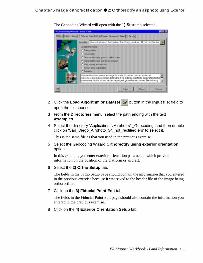
Chapter 6 Image orthorectification ● 2: Orthorectify an airphoto using Exterior
tered being
you
The Geocoding Wizard will open with the 1) Start tab selected.
2 Click the Load Algorithm or Dataset button in the Input file: field to open the file chooser.
3 From the Directories menu, select the path ending with the text \examples .
4 Select the directory ‘Applications\,Airphoto\1_Geocoding’ and then double-click on ‘San_Diego_Airphoto_34_not_rectified.ers’ to select it.
This is the same file as that you used in the previous exercise.
5 Select the Geocoding Wizard Orthorectify using exterior orientation option.
In this example, you enter exterior orientation parameters which provide information on the position of the platform or aircraft.
6 Select the 2) Ortho Setup tab.
The fields in the Ortho Setup page should contain the information that you enin the previous exercise because it was saved to the header file of the image orthorectified.
7 Click on the 3) Fiducial Point Edit tab.
The fields in the Fiducial Point Edit page should also contain the information entered in the previous exercise.
8 Click on the 4) Exterior Orientation Setup tab.
ER Mapper Workbook - Land Information 135
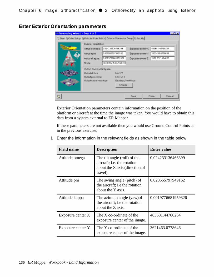
Chapter 6 Image orthorectification ● 2: Orthorectify an airphoto using Exterior
this
ts as
Enter Exterior Orientation parameters
Exterior Orientation parameters contain information on the position of the platform or aircraft at the time the image was taken. You would have to obtaindata from a system external to ER Mapper.
If these parameters are not available then you would use Ground Control Poinin the previous exercise.
1 Enter the information in the relevant fields as shown in the table below:
Field name Description Enter value
Attitude omega The tilt angle (roll) of the aircraft; i.e. the rotation about the X axis (direction of travel).
0.024233136466399
Attitude phi The swing angle (pitch) of the aircraft; i.e the rotation about the Y axis.
0.028555797949162
Attitude kappa The azimuth angle (yaw)of the aircraft; i.e the rotation about the Z axis.
0.0019776681959326
Exposure center X The X co-ordinate of the exposure center of the image.
483681.44788264
Exposure center Y The Y co-ordinate of the exposure center of the image.
3621463.0778646
136 ER Mapper Workbook - Land Information
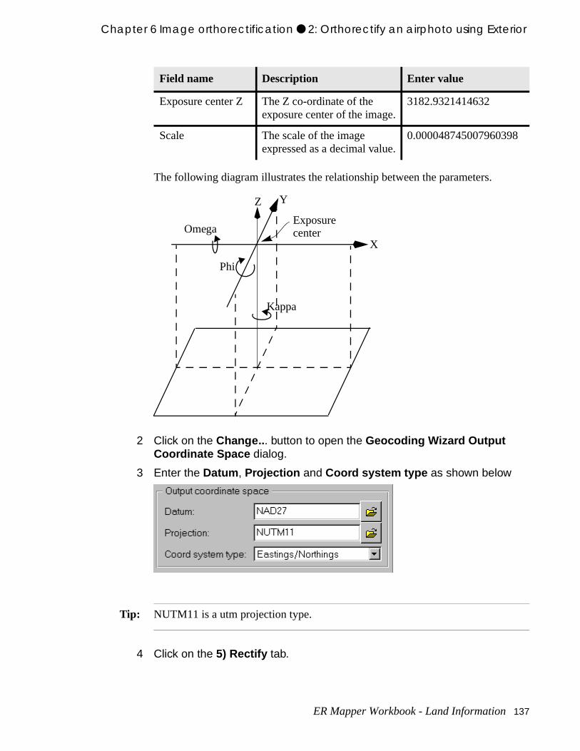
Chapter 6 Image orthorectification ● 2: Orthorectify an airphoto using Exterior
The following diagram illustrates the relationship between the parameters.
2 Click on the Change.. . button to open the Geocoding Wizard Output Coordinate Space dialog.
3 Enter the Datum , Projection and Coord system type as shown below
Tip: NUTM11 is a utm projection type.
4 Click on the 5) Rectify tab.
Exposure center Z The Z co-ordinate of the exposure center of the image.
3182.9321414632
Scale The scale of the image expressed as a decimal value.
0.000048745007960398
Field name Description Enter value
X
YZ
Exposurecenter
Kappa
Omega
Phi
ER Mapper Workbook - Land Information 137
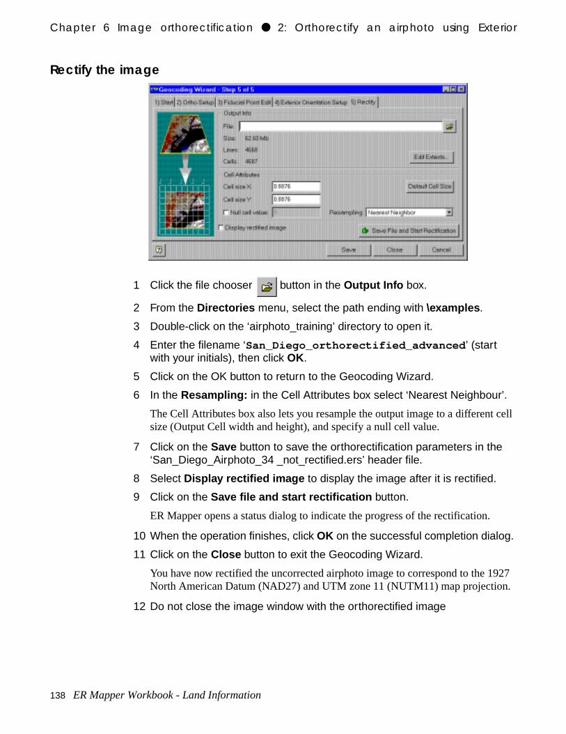
Chapter 6 Image orthorectification ● 2: Orthorectify an airphoto using Exterior
cell
927 .
Rectify the image
1 Click the file chooser button in the Output Info box.
2 From the Directories menu, select the path ending with \examples .
3 Double-click on the ‘airphoto_training’ directory to open it.
4 Enter the filename ‘San_Diego_orthorectified_advanced ’ (start with your initials), then click OK.
5 Click on the OK button to return to the Geocoding Wizard.
6 In the Resampling: in the Cell Attributes box select ‘Nearest Neighbour’.
The Cell Attributes box also lets you resample the output image to a differentsize (Output Cell width and height), and specify a null cell value.
7 Click on the Save button to save the orthorectification parameters in the ‘San_Diego_Airphoto_34 _not_rectified.ers’ header file.
8 Select Display rectified image to display the image after it is rectified.
9 Click on the Save file and start rectification button.
ER Mapper opens a status dialog to indicate the progress of the rectification.
10 When the operation finishes, click OK on the successful completion dialog.
11 Click on the Close button to exit the Geocoding Wizard.
You have now rectified the uncorrected airphoto image to correspond to the 1North American Datum (NAD27) and UTM zone 11 (NUTM11) map projection
12 Do not close the image window with the orthorectified image
138 ER Mapper Workbook - Land Information
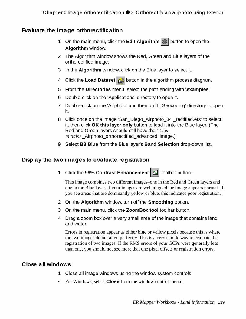
Chapter 6 Image orthorectification ● 2: Orthorectify an airphoto using Exterior
and al. If ion.
ere e s .
Evaluate the image orthorectification
1 On the main menu, click the Edit Algorithm button to open the Algorithm window.
2 The Algorithm window shows the Red, Green and Blue layers of the orthorectified image.
3 In the Algorithm window, click on the Blue layer to select it.
4 Click the Load Dataset button in the algorithm process diagram.
5 From the Directories menu, select the path ending with \examples .
6 Double-click on the ‘Applications’ directory to open it.
7 Double-click on the ‘Airphoto’ and then on ‘1_Geocoding’ directory to open it.
8 Click once on the image ‘San_Diego_Airphoto_34 _rectified.ers’ to select it, then click OK this layer only button to load it into the Blue layer. (The Red and Green layers should still have the ‘<your Initials>_Airphoto_orthorectified_advanced’ image.)
9 Select B3:Blue from the Blue layer’s Band Selection drop-down list.
Display the two images to evaluate registration
1 Click the 99% Contrast Enhancement toolbar button.
This image combines two different images–one in the Red and Green layers one in the Blue layer. If your images are well aligned the image appears normyou see areas that are dominantly yellow or blue, this indicates poor registrat
2 On the Algorithm window, turn off the Smoothing option.
3 On the main menu, click the ZoomBox tool toolbar button.
4 Drag a zoom box over a very small area of the image that contains land and water.
Errors in registration appear as either blue or yellow pixels because this is whthe two images do not align perfectly. This is a very simple way to evaluate thregistration of two images. If the RMS errors of your GCPs were generally lesthan one, you should not see more that one pixel offsets or registration errors
Close all windows1 Close all image windows using the window system controls:
• For Windows, select Close from the window control-menu.
ER Mapper Workbook - Land Information 139
Chapter 6 Image orthorectification ● 2: Orthorectify an airphoto using Exterior
ct
n
in
• For Unix systems, press right mouse button on the window title bar, and seleClose or Quit (for systems with both options, select Quit ).
2 Click Close on the Algorithm window to close it.
Only the ER Mapper main menu should be open on the screen.
• Use the Camera Wizard to create a Camera File
• Select fiducial markers on an airphoto image
• Use options to modify the GCP display and edit GCPs
• Enter Exterior Orientation parameters for advanced orthorectification.
• Use the Geocoding Wizard to orthorectify a “raw” airphoto image to the chosedatum and map projection.
What you learned...
After completing these exercises, you know how to perform the following tasksER Mapper:
140 ER Mapper Workbook - Land Information
more ches
.
eate this er a e in tion. are ther.
7
Assembling imagemosaics
This chapter explains how to create algorithms to display and process two or separate airphoto images as a mosaic. You will learn how ER Mapper approathe concept of creating mosaics and how to build an image mosaic algorithm
About assembling mosaicsThe term “mosaic” refers to assembling two or more overlapping images to cra continuous representation of the area covered by the images (a mosaic). Inexample, you will create a mosaic of several overlapping aerial photos to covlarger geographic area. The process of creating image mosaics is very simplER Mapper once the images are rectified to the same datum and map projecAny number of co-registered images used in the same processing algorithm automatically displayed in their correct geographic positions relative to each o
Requirements for mosaics
In order for ER Mapper to create a mosaic, each of the images must have thefollowing in common:
• they must be registered to the same geographic datum
• they must be registered to the same map projection
ER Mapper Workbook - Airphoto Mosaic Applications 141
Chapter 7#Assembling image mosaics#z Hands-on exercises
aics
for a
s, you ers curs
lay ts in
xtents er
of
• they must be rotated the same amount from north (if rotation is used).
You will learn how to rectify images to datums and map projections later.
Mosaic capabilities
Other than having a common datum and map projection, you can create mosthat contain very different types of data. An image mosaic can be built with datasets that have:
• different numbers of bands (i.e., three for a color airphoto versus seven Landsat satellite image)
• different data formats (i.e., byte format versus floating point format)
• different resolutions or cell sizes (i.e., 1-meter versus 3-meter).
Dataset display priority
By changing the order of the algorithm layers containing the separate datasetcan control dataset display priority (that is, which images appear on top of othin the event of overlap). Datasets loaded into the uppermost layer of any typealways appear on top of any other datasets in layers below where overlap ocbetween them.
Datasets loaded into the lowest layer of any type always have the lowest disppriority and will only be visible in areas where there is no overlap from dataselayers above them. For example, if you are creating a mosaic with a high resolution dataset and a lower resolution dataset, you can display the entire eof the high resolution dataset by putting its layer(s) on top in the algorithm laylist.
Note: Layer priority only applies to raster layers; vector layers always appear on topraster layers regardless of their position in the algorithm layer list.
Hands-on exercisesThese exercises show you how to create greyscale and RGB image mosaic algorithms.
142 ER Mapper Workbook - Airphoto Mosaic Applications
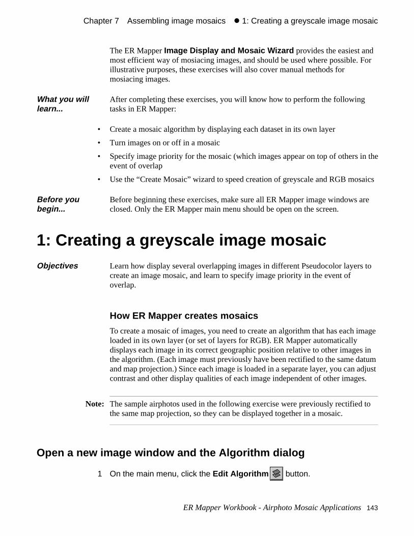
Chapter 7#Assembling image mosaics#z 1: Creating a greyscale image mosaic
For
n the
aics
image
s in atum adjust es.
to
are
to
The ER Mapper Image Display and Mosaic Wizard provides the easiest andmost efficient way of mosiacing images, and should be used where possible.illustrative purposes, these exercises will also cover manual methods for mosiacing images.
• Create a mosaic algorithm by displaying each dataset in its own layer
• Turn images on or off in a mosaic
• Specify image priority for the mosaic (which images appear on top of others ievent of overlap
• Use the “Create Mosaic” wizard to speed creation of greyscale and RGB mos
1: Creating a greyscale image mosaic
How ER Mapper creates mosaics
To create a mosaic of images, you need to create an algorithm that has eachloaded in its own layer (or set of layers for RGB). ER Mapper automatically displays each image in its correct geographic position relative to other imagethe algorithm. (Each image must previously have been rectified to the same dand map projection.) Since each image is loaded in a separate layer, you cancontrast and other display qualities of each image independent of other imag
Note: The sample airphotos used in the following exercise were previously rectifiedthe same map projection, so they can be displayed together in a mosaic.
Open a new image window and the Algorithm dialog
1 On the main menu, click the Edit Algorithm button.
What you will learn...
After completing these exercises, you will know how to perform the following tasks in ER Mapper:
Before you begin...
Before beginning these exercises, make sure all ER Mapper image windows closed. Only the ER Mapper main menu should be open on the screen.
Objectives Learn how display several overlapping images in different Pseudocolor layerscreate an image mosaic, and learn to specify image priority in the event of overlap.
ER Mapper Workbook - Airphoto Mosaic Applications 143
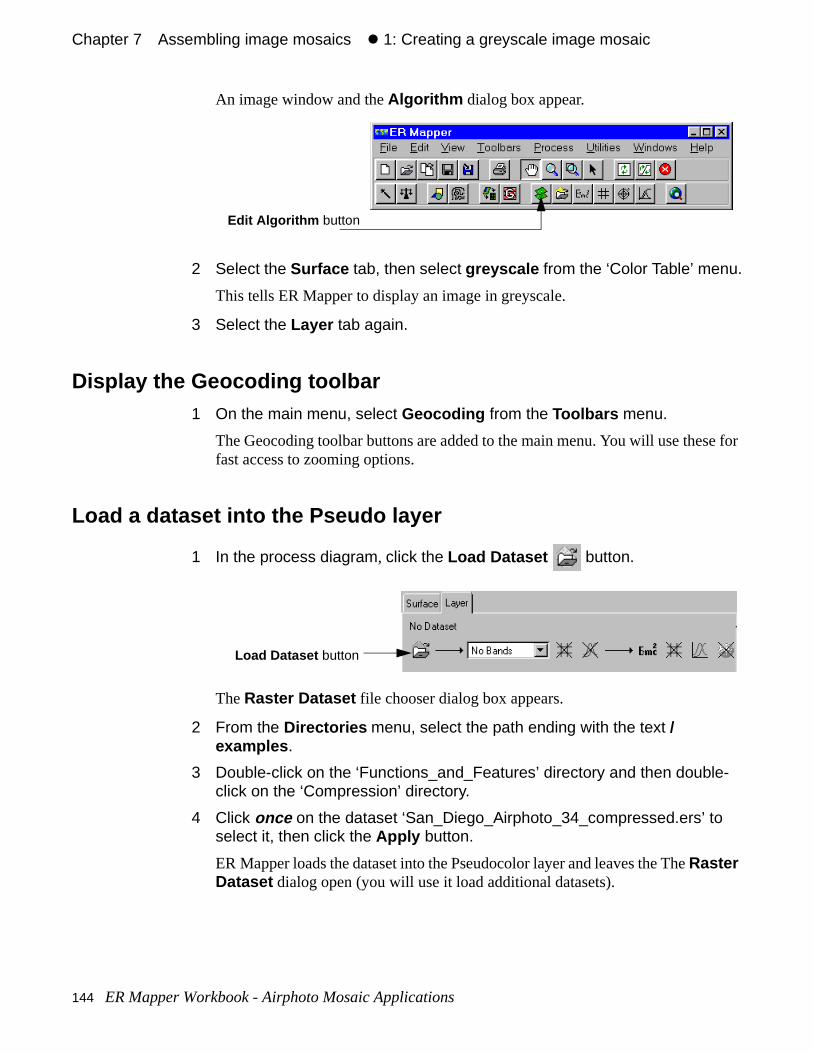
Chapter 7#Assembling image mosaics#z 1: Creating a greyscale image mosaic
e for
An image window and the Algorithm dialog box appear.
2 Select the Surface tab, then select greyscale from the ‘Color Table’ menu.
This tells ER Mapper to display an image in greyscale.
3 Select the Layer tab again.
Display the Geocoding toolbar1 On the main menu, select Geocoding from the Toolbars menu.
The Geocoding toolbar buttons are added to the main menu. You will use thesfast access to zooming options.
Load a dataset into the Pseudo layer
1 In the process diagram, click the Load Dataset button.
The Raster Dataset file chooser dialog box appears.
2 From the Directories menu, select the path ending with the text /examples .
3 Double-click on the ‘Functions_and_Features’ directory and then double-click on the ‘Compression’ directory.
4 Click once on the dataset ‘San_Diego_Airphoto_34_compressed.ers’ to select it, then click the Apply button.
ER Mapper loads the dataset into the Pseudocolor layer and leaves the The Raster Dataset dialog open (you will use it load additional datasets).
Edit Algorithm button
Load Dataset button
144 ER Mapper Workbook - Airphoto Mosaic Applications
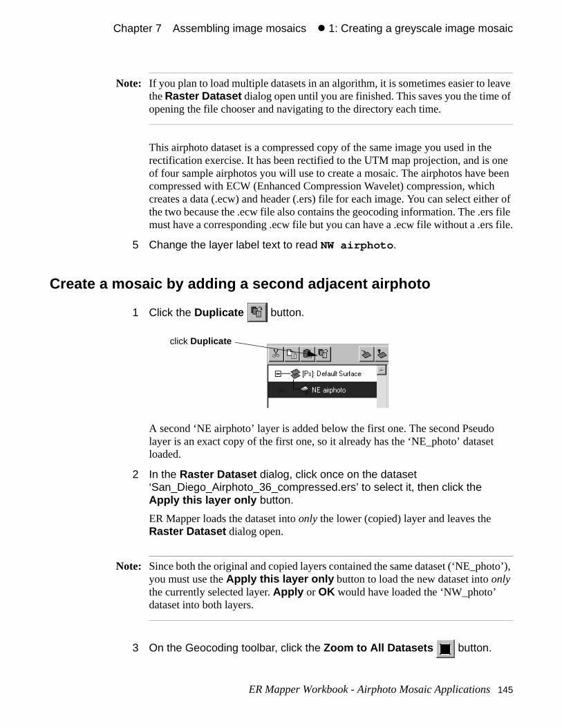
Chapter 7#Assembling image mosaics#z 1: Creating a greyscale image mosaic
eave of
e one been h ther of rs file s file.
o t
oto’),
Note: If you plan to load multiple datasets in an algorithm, it is sometimes easier to lthe Raster Dataset dialog open until you are finished. This saves you the timeopening the file chooser and navigating to the directory each time.
This airphoto dataset is a compressed copy of the same image you used in threctification exercise. It has been rectified to the UTM map projection, and is of four sample airphotos you will use to create a mosaic. The airphotos have compressed with ECW (Enhanced Compression Wavelet) compression, whiccreates a data (.ecw) and header (.ers) file for each image. You can select eithe two because the .ecw file also contains the geocoding information. The .emust have a corresponding .ecw file but you can have a .ecw file without a .er
5 Change the layer label text to read NW airphoto .
Create a mosaic by adding a second adjacent airphoto
1 Click the Duplicate button.
A second ‘NE airphoto’ layer is added below the first one. The second Pseudlayer is an exact copy of the first one, so it already has the ‘NE_photo’ dataseloaded.
2 In the Raster Dataset dialog, click once on the dataset ‘San_Diego_Airphoto_36_compressed.ers’ to select it, then click the Apply this layer only button.
ER Mapper loads the dataset into only the lower (copied) layer and leaves the Raster Dataset dialog open.
Note: Since both the original and copied layers contained the same dataset (‘NE_phyou must use the Apply this layer only button to load the new dataset into only the currently selected layer. Apply or OK would have loaded the ‘NW_photo’ dataset into both layers.
3 On the Geocoding toolbar, click the Zoom to All Datasets button.
click Duplicate
ER Mapper Workbook - Airphoto Mosaic Applications 145
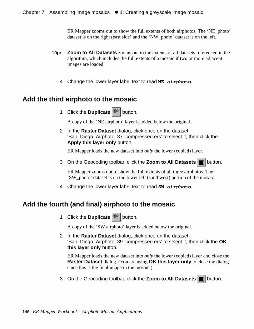
Chapter 7#Assembling image mosaics#z 1: Creating a greyscale image mosaic
oto’
the
ER Mapper zooms out to show the full extents of both airphotos. The ‘NE_phdataset is on the right (east side) and the ‘NW_photo’ dataset is on the left.
Tip: Zoom to All Datasets zooms out to the extents of all datasets referenced in algorithm, which includes the full extents of a mosaic if two or more adjacent images are loaded.
4 Change the lower layer label text to read NE airphoto .
Add the third airphoto to the mosaic
1 Click the Duplicate button.
A copy of the ‘NE airphoto’ layer is added below the original.
2 In the Raster Dataset dialog, click once on the dataset ‘San_Diego_Airphoto_37_compressed.ers’ to select it, then click the Apply this layer only button.
ER Mapper loads the new dataset into only the lower (copied) layer.
3 On the Geocoding toolbar, click the Zoom to All Datasets button.
ER Mapper zooms out to show the full extents of all three airphotos. The ‘SW_photo’ dataset is on the lower left (southwest) portion of the mosaic.
4 Change the lower layer label text to read SW airphoto .
Add the fourth (and final) airphoto to the mosaic
1 Click the Duplicate button.
A copy of the ‘SW airphoto’ layer is added below the original.
2 In the Raster Dataset dialog, click once on the dataset ‘San_Diego_Airphoto_39_compressed.ers’ to select it, then click the OK this layer only button.
ER Mapper loads the new dataset into only the lower (copied) layer and close theRaster Dataset dialog. (You are using OK this layer only to close the dialog since this is the final image in the mosaic.)
3 On the Geocoding toolbar, click the Zoom to All Datasets button.
146 ER Mapper Workbook - Airphoto Mosaic Applications
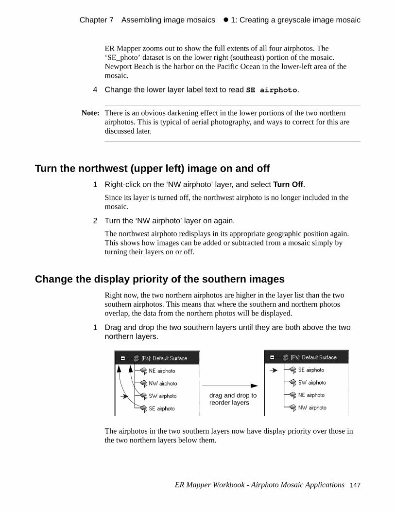
Chapter 7#Assembling image mosaics#z 1: Creating a greyscale image mosaic
e
e
n.
in
ER Mapper zooms out to show the full extents of all four airphotos. The ‘SE_photo’ dataset is on the lower right (southeast) portion of the mosaic. Newport Beach is the harbor on the Pacific Ocean in the lower-left area of themosaic.
4 Change the lower layer label text to read SE airphoto .
Note: There is an obvious darkening effect in the lower portions of the two northernairphotos. This is typical of aerial photography, and ways to correct for this ardiscussed later.
Turn the northwest (upper left) image on and off 1 Right-click on the ‘NW airphoto’ layer, and select Turn Off .
Since its layer is turned off, the northwest airphoto is no longer included in thmosaic.
2 Turn the ‘NW airphoto’ layer on again.
The northwest airphoto redisplays in its appropriate geographic position agaiThis shows how images can be added or subtracted from a mosaic simply byturning their layers on or off.
Change the display priority of the southern imagesRight now, the two northern airphotos are higher in the layer list than the two southern airphotos. This means that where the southern and northern photosoverlap, the data from the northern photos will be displayed.
1 Drag and drop the two southern layers until they are both above the two northern layers.
The airphotos in the two southern layers now have display priority over thosethe two northern layers below them.
drag and drop toreorder layers
ER Mapper Workbook - Airphoto Mosaic Applications 147
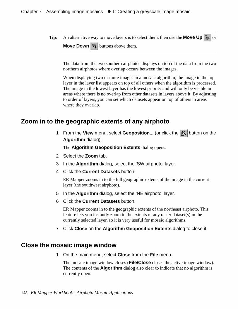
Chapter 7#Assembling image mosaics#z 1: Creating a greyscale image mosaic
two
top ssed.
usting s
t
s
Tip: An alternative way to move layers is to select them, then use the Move Up or
Move Down buttons above them.
The data from the two southern airphotos displays on top of the data from thenorthern airphotos where overlap occurs between the images.
When displaying two or more images in a mosaic algorithm, the image in thelayer in the layer list appears on top of all others when the algorithm is proceThe image in the lowest layer has the lowest priority and will only be visible inareas where there is no overlap from other datasets in layers above it. By adjto order of layers, you can set which datasets appear on top of others in areawhere they overlap.
Zoom in to the geographic extents of any airphoto
1 From the View menu, select Geoposition... (or click the button on the Algorithm dialog).
The Algorithm Geoposition Extents dialog opens.
2 Select the Zoom tab.
3 In the Algorithm dialog, select the ‘SW airphoto’ layer.
4 Click the Current Datasets button.
ER Mapper zooms in to the full geographic extents of the image in the currenlayer (the southwest airphoto).
5 In the Algorithm dialog, select the ‘NE airphoto’ layer.
6 Click the Current Datasets button.
ER Mapper zooms in to the geographic extents of the northeast airphoto. Thifeature lets you instantly zoom to the extents of any raster dataset(s) in the currently selected layer, so it is very useful for mosaic algorithms.
7 Click Close on the Algorithm Geoposition Extents dialog to close it.
Close the mosaic image window1 On the main menu, select Close from the File menu.
The mosaic image window closes (File/Close closes the active image window). The contents of the Algorithm dialog also clear to indicate that no algorithm is currently open.
148 ER Mapper Workbook - Airphoto Mosaic Applications
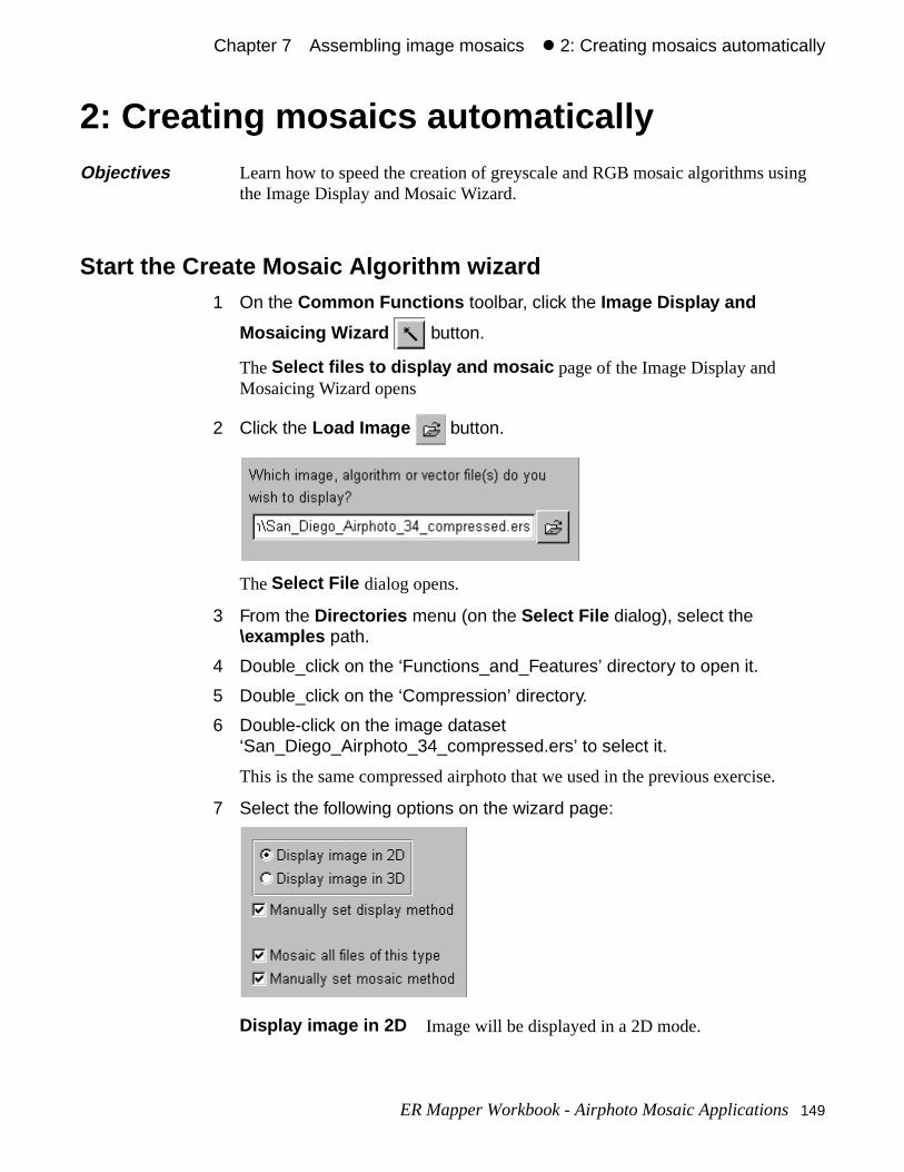
Chapter 7#Assembling image mosaics#z 2: Creating mosaics automatically
ing
2: Creating mosaics automatically
Start the Create Mosaic Algorithm wizard1 On the Common Functions toolbar, click the Image Display and
Mosaicing Wizard button.
The Select files to display and mosaic page of the Image Display and Mosaicing Wizard opens
2 Click the Load Image button.
The Select File dialog opens.
3 From the Directories menu (on the Select File dialog), select the \examples path.
4 Double_click on the ‘Functions_and_Features’ directory to open it.
5 Double_click on the ‘Compression’ directory.
6 Double-click on the image dataset ‘San_Diego_Airphoto_34_compressed.ers’ to select it.
This is the same compressed airphoto that we used in the previous exercise.
7 Select the following options on the wizard page:
Display image in 2D Image will be displayed in a 2D mode.
Objectives Learn how to speed the creation of greyscale and RGB mosaic algorithms usthe Image Display and Mosaic Wizard.
ER Mapper Workbook - Airphoto Mosaic Applications 149
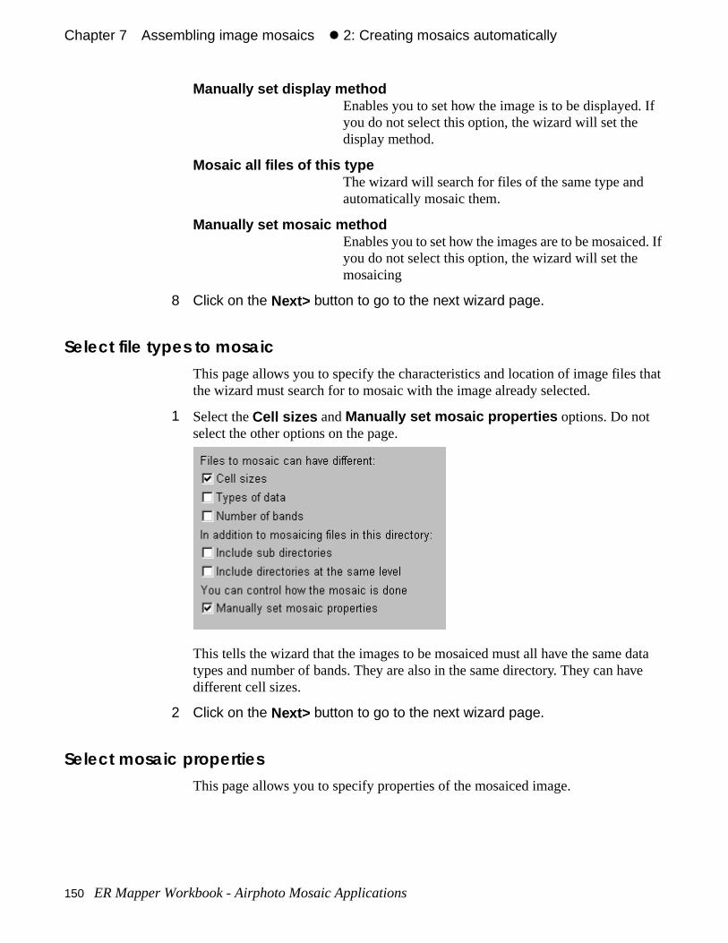
Chapter 7#Assembling image mosaics#z 2: Creating mosaics automatically
If
d. If
that
ata ve
Manually set display methodEnables you to set how the image is to be displayed.you do not select this option, the wizard will set the display method.
Mosaic all files of this typeThe wizard will search for files of the same type and automatically mosaic them.
Manually set mosaic methodEnables you to set how the images are to be mosaiceyou do not select this option, the wizard will set the mosaicing
8 Click on the Next> button to go to the next wizard page.
Select file types to mosaicThis page allows you to specify the characteristics and location of image filesthe wizard must search for to mosaic with the image already selected.
1 Select the Cell sizes and Manually set mosaic properties options. Do not select the other options on the page.
This tells the wizard that the images to be mosaiced must all have the same dtypes and number of bands. They are also in the same directory. They can hadifferent cell sizes.
2 Click on the Next> button to go to the next wizard page.
Select mosaic propertiesThis page allows you to specify properties of the mosaiced image.
150 ER Mapper Workbook - Airphoto Mosaic Applications
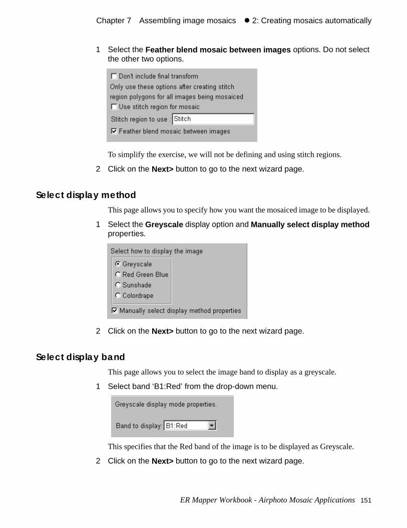
Chapter 7#Assembling image mosaics#z 2: Creating mosaics automatically
yed.
.
1 Select the Feather blend mosaic between images options. Do not select the other two options.
To simplify the exercise, we will not be defining and using stitch regions.
2 Click on the Next> button to go to the next wizard page.
Select display methodThis page allows you to specify how you want the mosaiced image to be displa
1 Select the Greyscale display option and Manually select display method properties.
2 Click on the Next> button to go to the next wizard page.
Select display bandThis page allows you to select the image band to display as a greyscale.
1 Select band ‘B1:Red’ from the drop-down menu.
This specifies that the Red band of the image is to be displayed as Greyscale
2 Click on the Next> button to go to the next wizard page.
ER Mapper Workbook - Airphoto Mosaic Applications 151
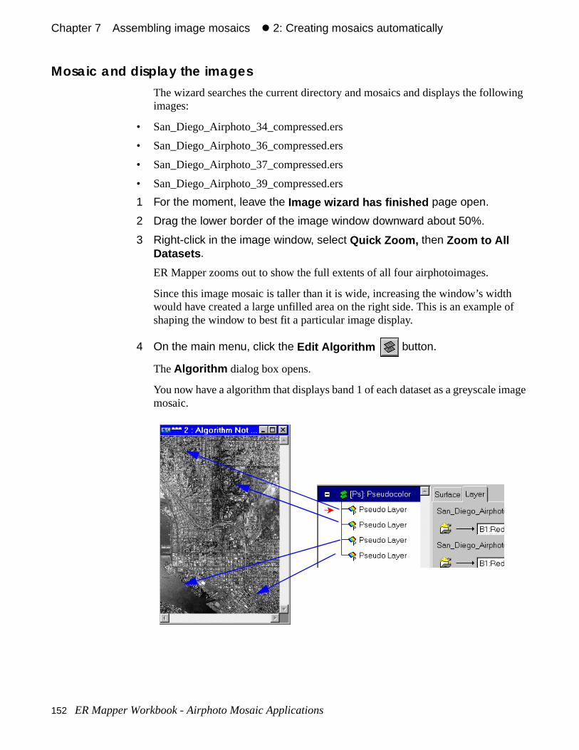
Chapter 7#Assembling image mosaics#z 2: Creating mosaics automatically
wing
of
image
Mosaic and display the imagesThe wizard searches the current directory and mosaics and displays the folloimages:
• San_Diego_Airphoto_34_compressed.ers
• San_Diego_Airphoto_36_compressed.ers
• San_Diego_Airphoto_37_compressed.ers
• San_Diego_Airphoto_39_compressed.ers
1 For the moment, leave the Image wizard has finished page open.
2 Drag the lower border of the image window downward about 50%.
3 Right-click in the image window, select Quick Zoom, then Zoom to All Datasets .
ER Mapper zooms out to show the full extents of all four airphotoimages.
Since this image mosaic is taller than it is wide, increasing the window’s widthwould have created a large unfilled area on the right side. This is an exampleshaping the window to best fit a particular image display.
4 On the main menu, click the Edit Algorithm button.
The Algorithm dialog box opens.
You now have a algorithm that displays band 1 of each dataset as a greyscalemosaic.
152 ER Mapper Workbook - Airphoto Mosaic Applications
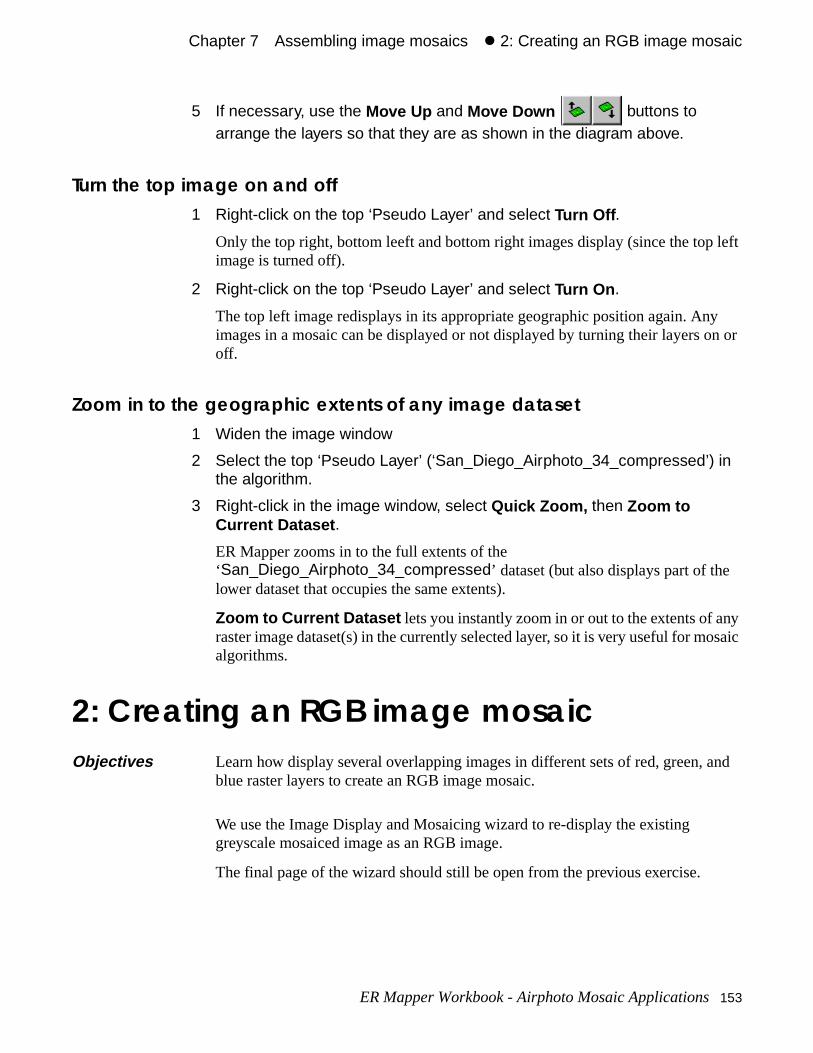
Chapter 7#Assembling image mosaics#z 2: Creating an RGB image mosaic
left
y on or
ny osaic
and
5 If necessary, use the Move Up and Move Down buttons to arrange the layers so that they are as shown in the diagram above.
Turn the top image on and off 1 Right-click on the top ‘Pseudo Layer’ and select Turn Off .
Only the top right, bottom leeft and bottom right images display (since the topimage is turned off).
2 Right-click on the top ‘Pseudo Layer’ and select Turn On .
The top left image redisplays in its appropriate geographic position again. Animages in a mosaic can be displayed or not displayed by turning their layers off.
Zoom in to the geographic extents of any image dataset1 Widen the image window
2 Select the top ‘Pseudo Layer’ (‘San_Diego_Airphoto_34_compressed’) in the algorithm.
3 Right-click in the image window, select Quick Zoom, then Zoom to Current Dataset .
ER Mapper zooms in to the full extents of the ‘San_Diego_Airphoto_34_compressed’ dataset (but also displays part of thelower dataset that occupies the same extents).
Zoom to Current Dataset lets you instantly zoom in or out to the extents of araster image dataset(s) in the currently selected layer, so it is very useful for malgorithms.
2: Creating an RGB image mosaic
We use the Image Display and Mosaicing wizard to re-display the existing greyscale mosaiced image as an RGB image.
The final page of the wizard should still be open from the previous exercise.
Objectives Learn how display several overlapping images in different sets of red, green, blue raster layers to create an RGB image mosaic.
ER Mapper Workbook - Airphoto Mosaic Applications 153
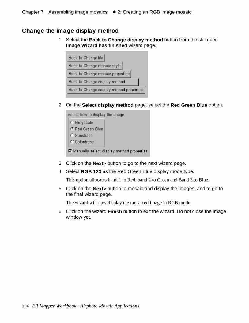
Chapter 7#Assembling image mosaics#z 2: Creating an RGB image mosaic
Change the image display method1 Select the Back to Change display method button from the still open
Image Wizard has finished wizard page.
2 On the Select display method page, select the Red Green Blue option.
3 Click on the Next> button to go to the next wizard page.
4 Select RGB 123 as the Red Green Blue display mode type.
This option allocates band 1 to Red. band 2 to Green and Band 3 to Blue.
5 Click on the Next> button to mosaic and display the images, and to go to the final wizard page.
The wizard will now display the mosaiced image in RGB mode.
6 Click on the wizard Finish button to exit the wizard. Do not close the image window yet.
154 ER Mapper Workbook - Airphoto Mosaic Applications
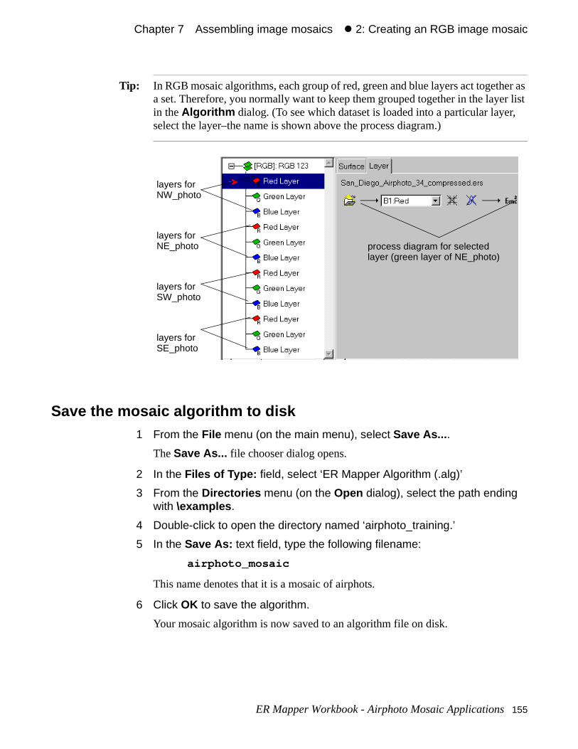
Chapter 7#Assembling image mosaics#z 2: Creating an RGB image mosaic
her as r list
r,
Tip: In RGB mosaic algorithms, each group of red, green and blue layers act togeta set. Therefore, you normally want to keep them grouped together in the layein the Algorithm dialog. (To see which dataset is loaded into a particular layeselect the layer–the name is shown above the process diagram.)
Save the mosaic algorithm to disk1 From the File menu (on the main menu), select Save As... .
The Save As... file chooser dialog opens.
2 In the Files of Type: field, select ‘ER Mapper Algorithm (.alg)’
3 From the Directories menu (on the Open dialog), select the path ending with \examples .
4 Double-click to open the directory named ‘airphoto_training.’
5 In the Save As: text field, type the following filename:
airphoto_mosaic
This name denotes that it is a mosaic of airphots.
6 Click OK to save the algorithm.
Your mosaic algorithm is now saved to an algorithm file on disk.
layers forNW_photo
layers forNE_photo
layers forSW_photo
layers forSE_photo
process diagram for selectedlayer (green layer of NE_photo)
ER Mapper Workbook - Airphoto Mosaic Applications 155
Chapter 7#Assembling image mosaics#z 2: Creating an RGB image mosaic
n the
aics
s
Close all image windows and dialog boxes1 Close both image windows by selecting Close from the File menu.
2 Click Close on the Algorithm dialog to close it.
Only the ER Mapper main menu should be open on the screen.
• Create a mosaic algorithm by displaying each dataset in its own layer
• Turn images on or off in a mosaic
• Specify image priority for the mosaic (which images appear on top of others ievent of overlap
• Use the “Create Mosaic” wizard to speed creation of greyscale and RGB mos
What you learned
After completing these exercises, you know how to perform the following taskin ER Mapper:
156 ER Mapper Workbook - Airphoto Mosaic Applications
ss darker c of
ssed
d this g
ages
8
Color balancingimages
This chapter explains techniques to correct or normalize changes in brightneacross single images that cause some areas to appear noticeably brighter orthan others. It also discusses ways to balance the overall contrast of a mosaiimages to make them appear as a single image.
About color balancingWhen creating a mosaic of images, there are two primary issues to be addrethat help make the mosaic appear to be a single, seamless image:
Note: The Color Balancing Wizard balances and matches colors automatically, andoes not require any manual intervention. The descriptions and exercises in chapter have been included to provide an understanding of the color balancinprocess.
• correcting shifts in brightness or color within individual images
• balancing the overall contrast of the mosaic (normalizing the contrast of all imto a common level)
ER Mapper Workbook - Airphoto Mosaic Applications 157
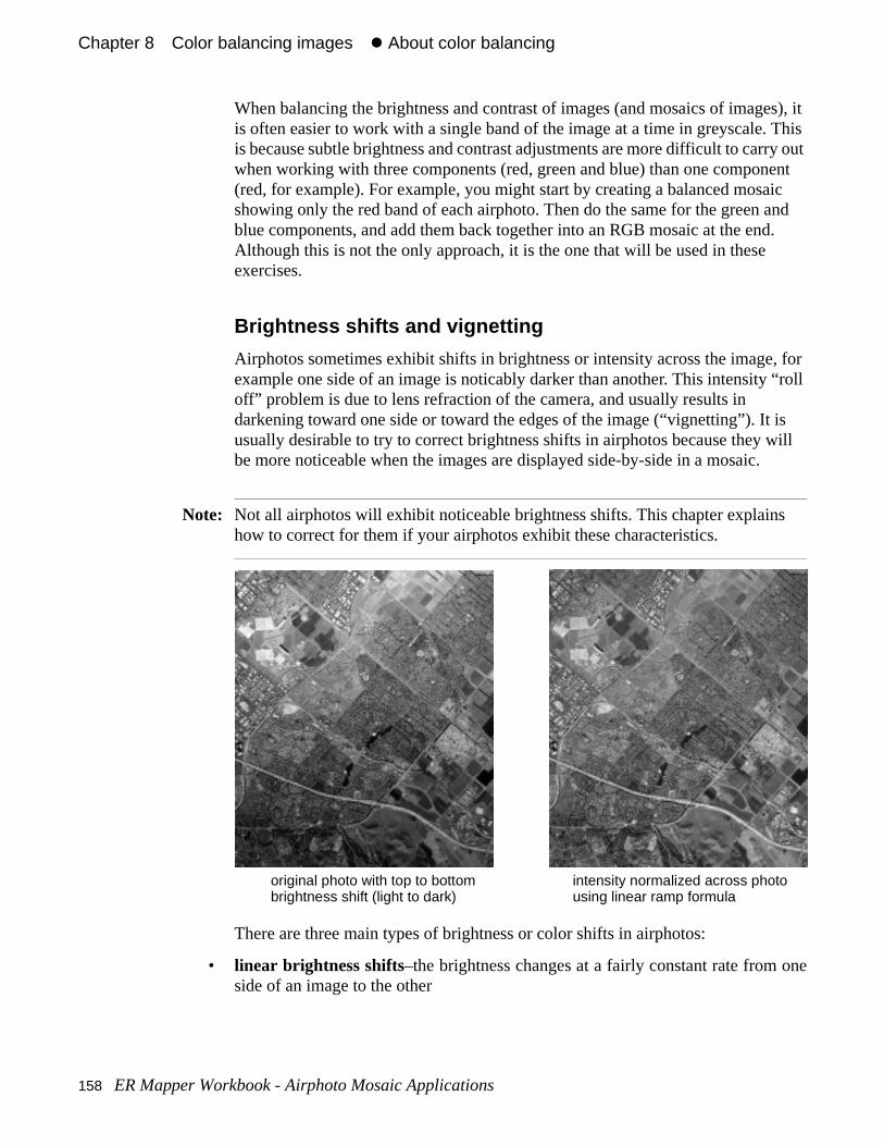
Chapter 8#Color balancing images#z About color balancing
es), it This ry out ent ic and d.
, for “roll
is will
s
one
When balancing the brightness and contrast of images (and mosaics of imagis often easier to work with a single band of the image at a time in greyscale.is because subtle brightness and contrast adjustments are more difficult to carwhen working with three components (red, green and blue) than one compon(red, for example). For example, you might start by creating a balanced mosashowing only the red band of each airphoto. Then do the same for the green blue components, and add them back together into an RGB mosaic at the enAlthough this is not the only approach, it is the one that will be used in these exercises.
Brightness shifts and vignetting
Airphotos sometimes exhibit shifts in brightness or intensity across the imageexample one side of an image is noticably darker than another. This intensityoff” problem is due to lens refraction of the camera, and usually results in darkening toward one side or toward the edges of the image (“vignetting”). It usually desirable to try to correct brightness shifts in airphotos because they be more noticeable when the images are displayed side-by-side in a mosaic.
Note: Not all airphotos will exhibit noticeable brightness shifts. This chapter explainhow to correct for them if your airphotos exhibit these characteristics.
There are three main types of brightness or color shifts in airphotos:
• linear brightness shifts–the brightness changes at a fairly constant rate from side of an image to the other
original photo with top to bottombrightness shift (light to dark)
intensity normalized across photousing linear ramp formula
158 ER Mapper Workbook - Airphoto Mosaic Applications
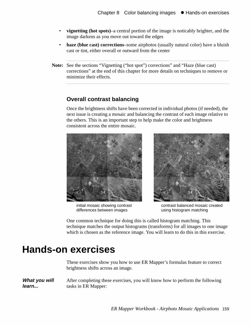
Chapter 8#Color balancing images#z Hands-on exercises
the
ish
ve or
), the tive to
age ise.
ct
• vignetting (hot spots)–a central portion of the image is noticably brighter, and image darkens as you move out toward the edges
• haze (blue cast) corrections–some airphotos (usually natural color) have a blucast or tint, either overall or outward from the center
Note: See the sections “Vignetting (“hot spot”) corrections” and “Haze (blue cast) corrections” at the end of this chapter for more details on techniques to remominimize their effects.
Overall contrast balancing
Once the brightness shifts have been corrected in individual photos (if needednext issue is creating a mosaic and balancing the contrast of each image relathe others. This is an important step to help make the color and brightness consistent across the entire mosaic.
One common technique for doing this is called histogram matching. This technique matches the output histograms (transforms) for all images to one imwhich is chosen as the reference image. You will learn to do this in this exerc
Hands-on exercisesThese exercises show you how to use ER Mapper’s formulas feature to correbrightness shifts across an image.
What you will learn...
After completing these exercises, you will know how to perform the following tasks in ER Mapper:
initial mosaic showing contrastdifferences between images
contrast balanced mosaic createdusing histogram matching
ER Mapper Workbook - Airphoto Mosaic Applications 159
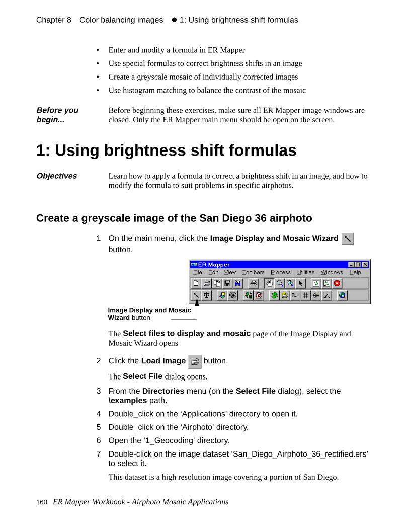
Chapter 8#Color balancing images#z 1: Using brightness shift formulas
are
to
• Enter and modify a formula in ER Mapper
• Use special formulas to correct brightness shifts in an image
• Create a greyscale mosaic of individually corrected images
• Use histogram matching to balance the contrast of the mosaic
1: Using brightness shift formulas
Create a greyscale image of the San Diego 36 airphoto
1 On the main menu, click the Image Display and Mosaic Wizard button.
The Select files to display and mosaic page of the Image Display and Mosaic Wizard opens
2 Click the Load Image button.
The Select File dialog opens.
3 From the Directories menu (on the Select File dialog), select the \examples path.
4 Double_click on the ‘Applications’ directory to open it.
5 Double_click on the ‘Airphoto’ directory.
6 Open the ‘1_Geocoding’ directory.
7 Double-click on the image dataset ‘San_Diego_Airphoto_36_rectified.ers’ to select it.
This dataset is a high resolution image covering a portion of San Diego.
Before you begin...
Before beginning these exercises, make sure all ER Mapper image windows closed. Only the ER Mapper main menu should be open on the screen.
Objectives Learn how to apply a formula to correct a brightness shift in an image, and howmodify the formula to suit problems in specific airphotos.
Image Display and MosaicWizard button
160 ER Mapper Workbook - Airphoto Mosaic Applications
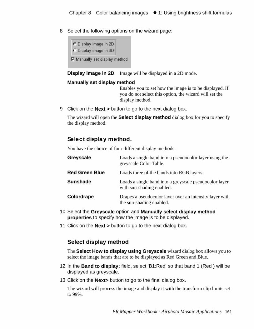
Chapter 8#Color balancing images#z 1: Using brightness shift formulas
If
e
er
th
set
8 Select the following options on the wizard page:
Display image in 2D Image will be displayed in a 2D mode.
Manually set display methodEnables you to set how the image is to be displayed.you do not select this option, the wizard will set the display method.
9 Click on the Next > button to go to the next dialog box.
The wizard will open the Select display method dialog box for you to specify the display method.
Select display method.You have the choice of four different display methods:
Greyscale Loads a single band into a pseudocolor layer using thgreyscale Color Table.
Red Green Blue Loads three of the bands into RGB layers.
Sunshade Loads a single band into a greyscale pseudocolor laywith sun-shading enabled.
Colordrape Drapes a pseudocolor layer over an intensity layer withe sun-shading enabled.
10 Select the Greyscale option and Manually select display method properties to specify how the image is to be displayed.
11 Click on the Next > button to go to the next dialog box.
Select display method
The Select How to display using Greyscale wizard dialog box allows you to select the image bands that are to be displayed as Red Green and Blue.
12 In the Band to display: field, select ‘B1:Red’ so that band 1 (Red ) will be displayed as greyscale.
13 Click on the Next> button to go to the final dialog box.
The wizard will process the image and display it with the transform clip limits to 99%.
ER Mapper Workbook - Airphoto Mosaic Applications 161
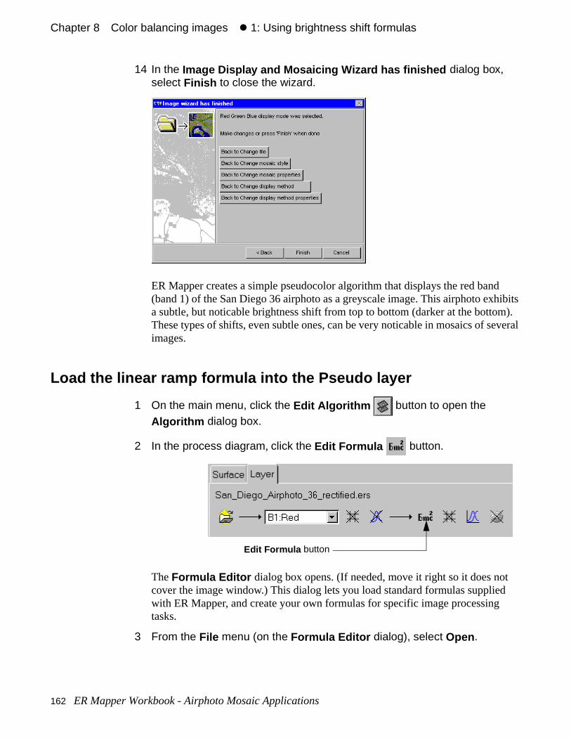
Chapter 8#Color balancing images#z 1: Using brightness shift formulas
d hibits m). everal
t d
14 In the Image Display and Mosaicing Wizard has finished dialog box, select Finish to close the wizard.
ER Mapper creates a simple pseudocolor algorithm that displays the red ban(band 1) of the San Diego 36 airphoto as a greyscale image. This airphoto exa subtle, but noticable brightness shift from top to bottom (darker at the bottoThese types of shifts, even subtle ones, can be very noticable in mosaics of simages.
Load the linear ramp formula into the Pseudo layer
1 On the main menu, click the Edit Algorithm button to open the
Algorithm dialog box.
2 In the process diagram, click the Edit Formula button.
The Formula Editor dialog box opens. (If needed, move it right so it does nocover the image window.) This dialog lets you load standard formulas suppliewith ER Mapper, and create your own formulas for specific image processingtasks.
3 From the File menu (on the Formula Editor dialog), select Open .
Edit Formula button
162 ER Mapper Workbook - Airphoto Mosaic Applications
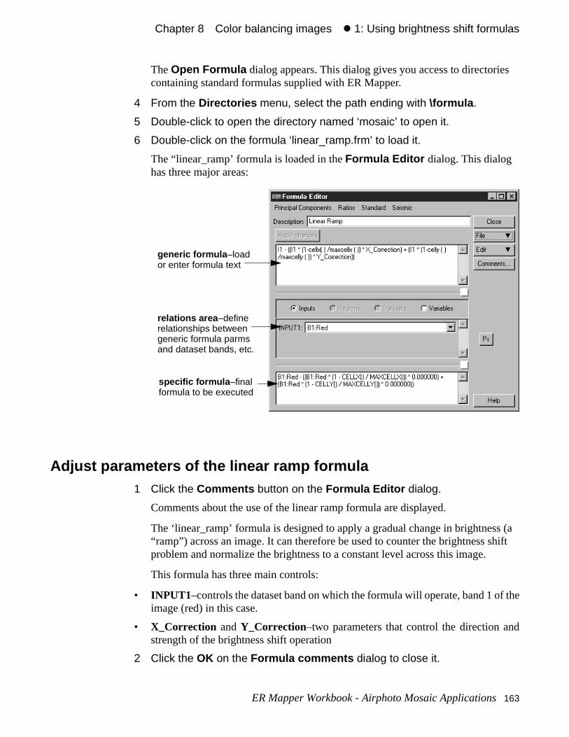
Chapter 8#Color balancing images#z 1: Using brightness shift formulas
s
s (a hift
f the
nd
The Open Formula dialog appears. This dialog gives you access to directoriecontaining standard formulas supplied with ER Mapper.
4 From the Directories menu, select the path ending with \formula .
5 Double-click to open the directory named ‘mosaic’ to open it.
6 Double-click on the formula ‘linear_ramp.frm’ to load it.
The “linear_ramp’ formula is loaded in the Formula Editor dialog. This dialog has three major areas:
Adjust parameters of the linear ramp formula1 Click the Comments button on the Formula Editor dialog.
Comments about the use of the linear ramp formula are displayed.
The ‘linear_ramp’ formula is designed to apply a gradual change in brightnes“ramp”) across an image. It can therefore be used to counter the brightness sproblem and normalize the brightness to a constant level across this image.
This formula has three main controls:
• INPUT1–controls the dataset band on which the formula will operate, band 1 oimage (red) in this case.
• X_Correction and Y_Correction–two parameters that control the direction astrength of the brightness shift operation
2 Click the OK on the Formula comments dialog to close it.
generic formula –loador enter formula text
relations area –definerelationships between
specific formula –finalformula to be executed
generic formula parmsand dataset bands, etc.
ER Mapper Workbook - Airphoto Mosaic Applications 163
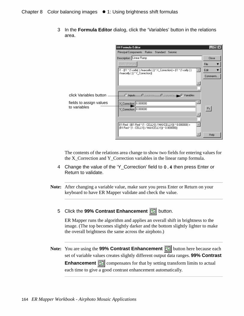
Chapter 8#Color balancing images#z 1: Using brightness shift formulas
s for
r
ke
3 In the Formula Editor dialog, click the ‘Variables’ button in the relations area.
The contents of the relations area change to show two fields for entering valuethe X_Correction and Y_Correction variables in the linear ramp formula.
4 Change the value of the ‘Y_Correction’ field to 0.4 then press Enter or Return to validate.
Note: After changing a variable value, make sure you press Enter or Return on youkeyboard to have ER Mapper validate and check the value.
5 Click the 99% Contrast Enhancement button.
ER Mapper runs the algorithm and applies an overall shift in brightness to theimage. (The top becomes slightly darker and the bottom slightly lighter to mathe overall brightness the same across the airphoto.)
Note: You are using the 99% Contrast Enhancement button here because each
set of variable values creates slightly different output data ranges. 99% Contrast
Enhancement compensates for that by setting transform limits to actual
each time to give a good contrast enhancement automatically.
click Variables button
fields to assign valuesto variables
164 ER Mapper Workbook - Airphoto Mosaic Applications
Chapter 8#Color balancing images#z 1: Using brightness shift formulas
ness , be
ge.
Try other correction values to see how the formula worksThe linear ramp formula is very versatile and can be used to adjust the brightshifts top-to-bottom, side-to-side, and diagonally across an image. To do thisadjust the values for X_CORRECTION and/or Y_CORRECTION variables asneeded. Suggested values range from 0.4 to -0.4, but larger values may alsouseful.
X_Correction - adjust brightness in the left to right direction: Example: 0.3 lightens the right side relative to left, -0.3 the opposite.
Y_Correction - adjust brightness in the top to bottom direction: Example: 0.3 lightens the bottom relative to top, -0.3 the opposite.
By using both variables, you can adjust brightness diagonally across the ima
1 Change the variable values as follows (press Return or Enter after):
X_Correction = 0.4
Y_Correction = 0.0
2 Click the 99% Contrast Enhancement button.
The right side of the image lightens relative to the left.
3 Change the variable values as follows (press Return or Enter after):
X_Correction = 0.4
Y_Correction = 0.4
4 Click the 99% Contrast Enhancement button.
The lower-right corner of the image lightens relative to the upper-left.
5 Change the variable values as follows (press Return or Enter after):
X_Correction = -0.4
Y_Correction = -0.4
6 Click the 99% Contrast Enhancement button.
The upper-left corner of the image lightens relative to the lower right.
Reset the correction values to the best for this image1 Change the variable values as follows (press Return or Enter after):
X_Correction = 0.0
Y_Correction = 0.4
ER Mapper Workbook - Airphoto Mosaic Applications 165
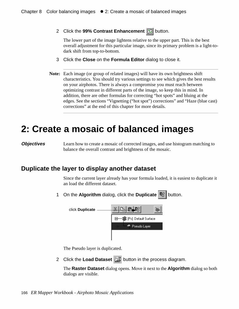
Chapter 8#Color balancing images#z 2: Create a mosaic of balanced images
t t-to-
sults
ast)
ate it
ng to
2 Click the 99% Contrast Enhancement button.
The lower part of the image lightens relative to the upper part. This is the besoverall adjustment for this particular image, since its primary problem is a lighdark shift from top-to-bottom.
3 Click the Close on the Formula Editor dialog to close it.
Note: Each image (or group of related images) will have its own brightness shift characteristics. You should try various settings to see which gives the best reon your airphotos. There is always a compromise you must reach between optimizing contrast in different parts of the image, so keep this in mind. In addition, there are other formulas for correcting “hot spots” and bluing at the edges. See the sections “Vignetting (“hot spot”) corrections” and “Haze (blue ccorrections” at the end of this chapter for more details.
2: Create a mosaic of balanced images
Duplicate the layer to display another datasetSince the current layer already has your formula loaded, it is easiest to duplican load the different dataset.
1 On the Algorithm dialog, click the Duplicate button.
The Pseudo layer is duplicated.
2 Click the Load Dataset button in the process diagram.
The Raster Dataset dialog opens. Move it next to the Algorithm dialog so both dialogs are visible.
Objectives Learn how to create a mosaic of corrected images, and use histogram matchibalance the overall contrast and brightness of the mosaic.
click Duplicate
166 ER Mapper Workbook - Airphoto Mosaic Applications
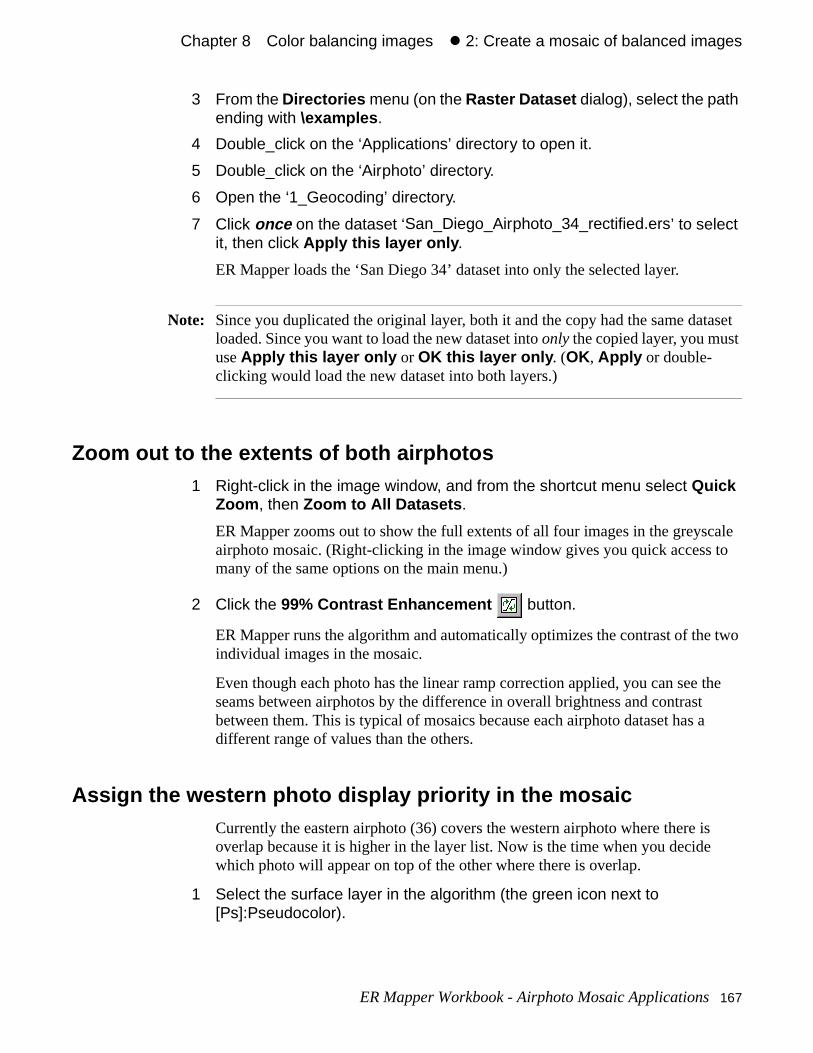
Chapter 8#Color balancing images#z 2: Create a mosaic of balanced images
taset
ale to
two
the a
s
3 From the Directories menu (on the Raster Dataset dialog), select the path ending with \examples .
4 Double_click on the ‘Applications’ directory to open it.
5 Double_click on the ‘Airphoto’ directory.
6 Open the ‘1_Geocoding’ directory.
7 Click once on the dataset ‘San_Diego_Airphoto_34_rectified.ers’ to select it, then click Apply this layer only .
ER Mapper loads the ‘San Diego 34’ dataset into only the selected layer.
Note: Since you duplicated the original layer, both it and the copy had the same daloaded. Since you want to load the new dataset into only the copied layer, you mustuse Apply this layer only or OK this layer only . (OK, Apply or double-clicking would load the new dataset into both layers.)
Zoom out to the extents of both airphotos1 Right-click in the image window, and from the shortcut menu select Quick
Zoom , then Zoom to All Datasets .
ER Mapper zooms out to show the full extents of all four images in the greyscairphoto mosaic. (Right-clicking in the image window gives you quick access many of the same options on the main menu.)
2 Click the 99% Contrast Enhancement button.
ER Mapper runs the algorithm and automatically optimizes the contrast of theindividual images in the mosaic.
Even though each photo has the linear ramp correction applied, you can seeseams between airphotos by the difference in overall brightness and contrastbetween them. This is typical of mosaics because each airphoto dataset has different range of values than the others.
Assign the western photo display priority in the mosaicCurrently the eastern airphoto (36) covers the western airphoto where there ioverlap because it is higher in the layer list. Now is the time when you decidewhich photo will appear on top of the other where there is overlap.
1 Select the surface layer in the algorithm (the green icon next to [Ps]:Pseudocolor).
ER Mapper Workbook - Airphoto Mosaic Applications 167
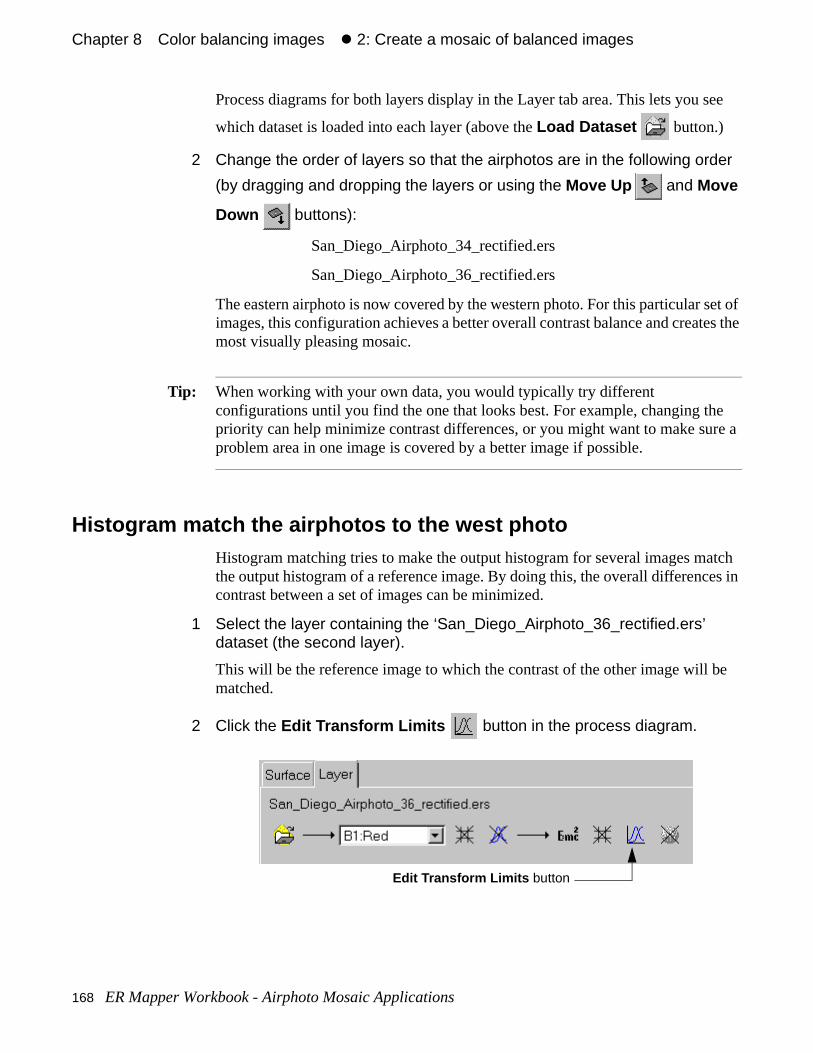
Chapter 8#Color balancing images#z 2: Create a mosaic of balanced images
see
set of tes the
e re a
atch es in
be
Process diagrams for both layers display in the Layer tab area. This lets you
which dataset is loaded into each layer (above the Load Dataset button.)
2 Change the order of layers so that the airphotos are in the following order
(by dragging and dropping the layers or using the Move Up and Move
Down buttons):
San_Diego_Airphoto_34_rectified.ers
San_Diego_Airphoto_36_rectified.ers
The eastern airphoto is now covered by the western photo. For this particular images, this configuration achieves a better overall contrast balance and creamost visually pleasing mosaic.
Tip: When working with your own data, you would typically try different configurations until you find the one that looks best. For example, changing thpriority can help minimize contrast differences, or you might want to make suproblem area in one image is covered by a better image if possible.
Histogram match the airphotos to the west photoHistogram matching tries to make the output histogram for several images mthe output histogram of a reference image. By doing this, the overall differenccontrast between a set of images can be minimized.
1 Select the layer containing the ‘San_Diego_Airphoto_36_rectified.ers’ dataset (the second layer).
This will be the reference image to which the contrast of the other image will matched.
2 Click the Edit Transform Limits button in the process diagram.
Edit Transform Limits button
168 ER Mapper Workbook - Airphoto Mosaic Applications
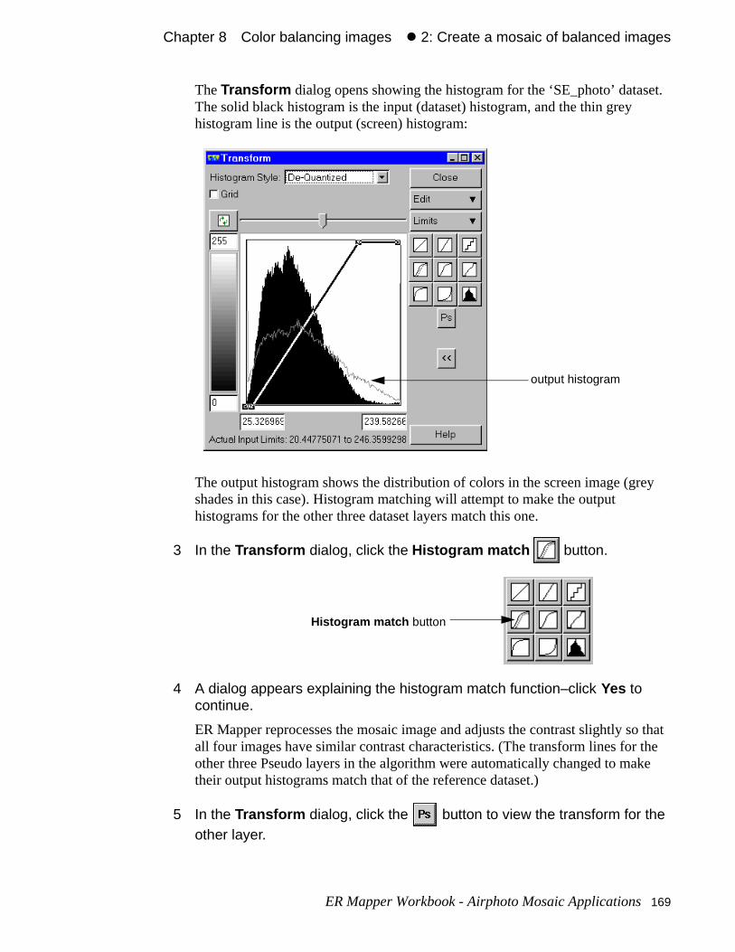
Chapter 8#Color balancing images#z 2: Create a mosaic of balanced images
et.
ey
o that the ke
The Transform dialog opens showing the histogram for the ‘SE_photo’ datasThe solid black histogram is the input (dataset) histogram, and the thin grey histogram line is the output (screen) histogram:
The output histogram shows the distribution of colors in the screen image (grshades in this case). Histogram matching will attempt to make the output histograms for the other three dataset layers match this one.
3 In the Transform dialog, click the Histogram match button.
4 A dialog appears explaining the histogram match function–click Yes to continue.
ER Mapper reprocesses the mosaic image and adjusts the contrast slightly sall four images have similar contrast characteristics. (The transform lines for other three Pseudo layers in the algorithm were automatically changed to matheir output histograms match that of the reference dataset.)
5 In the Transform dialog, click the button to view the transform for the other layer.
output histogram
Histogram match button
ER Mapper Workbook - Airphoto Mosaic Applications 169
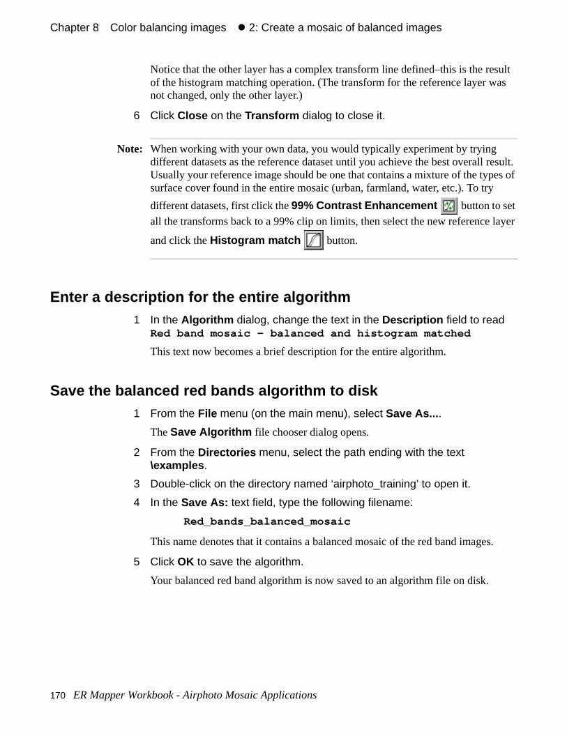
Chapter 8#Color balancing images#z 2: Create a mosaic of balanced images
sult as
result. es of
layer
s.
Notice that the other layer has a complex transform line defined–this is the reof the histogram matching operation. (The transform for the reference layer wnot changed, only the other layer.)
6 Click Close on the Transform dialog to close it.
Note: When working with your own data, you would typically experiment by trying different datasets as the reference dataset until you achieve the best overall Usually your reference image should be one that contains a mixture of the typsurface cover found in the entire mosaic (urban, farmland, water, etc.). To try
different datasets, first click the 99% Contrast Enhancement button to set
all the transforms back to a 99% clip on limits, then select the new reference
and click the Histogram match button.
Enter a description for the entire algorithm1 In the Algorithm dialog, change the text in the Description field to read
Red band mosaic - balanced and histogram matched
This text now becomes a brief description for the entire algorithm.
Save the balanced red bands algorithm to disk1 From the File menu (on the main menu), select Save As... .
The Save Algorithm file chooser dialog opens.
2 From the Directories menu, select the path ending with the text \examples .
3 Double-click on the directory named ‘airphoto_training’ to open it.
4 In the Save As: text field, type the following filename:
Red_bands_balanced_mosaic
This name denotes that it contains a balanced mosaic of the red band image
5 Click OK to save the algorithm.
Your balanced red band algorithm is now saved to an algorithm file on disk.
170 ER Mapper Workbook - Airphoto Mosaic Applications
Chapter 8#Color balancing images#z 2: Create a mosaic of balanced images
f the ove
he RGB
ess s. al
e
he ted
s
Tip: You will also have to define similar algorithms for the green and blue bands oimage mosaic. Since you will next perform some other processing to help remseam lines, it is easier to do this first to the red band mosaic, then duplicate tprocessing for the green and blue band mosaics before assembling the final color mosaic.
Close all image windows and dialog boxes1 Close the image window by selecting Close from the File menu.
2 Click Close on the Algorithm dialog to close it.
Only the ER Mapper main menu should be open on the screen.
• Enter and modify a formula in ER Mapper
• Use special formulas to correct brightness shifts in an image
• Create a greyscale mosaic of individually corrected images
• Use histogram matching to balance the contrast of the mosaic
Other color shift correctionsIn the previous exercise, you used the ‘linear_ramp’ formula to correct brightnshifts because that was the appropriate adjustment for the four sample imageHowever, there are also corrections for vignetting and haze (blue cast) removthat you may consider using if your airphotos exhibit these problems.
Vignetting (“hot spot”) correctionsInstead of a gradual shift in brightness or color from one side to another, somairphotos have a general darkening toward the edges outward from a centralbrighter area (the “hot spot”). This effect is called vignetting, and is due to lens refraction in the camera. (Special antivignette filters are sometimes used on tcamera to minimize this effect.) This type of correction is a bit more complicamathematically, but is still fairly easy to implement in ER Mapper.
To use the hot spot formula technique, first display your image in an RGB algorithm, then follow these steps:
1 Select Cell Coordinate from the View menu.
What you learned
After completing these exercises, you know how to perform the following taskin ER Mapper:
ER Mapper Workbook - Airphoto Mosaic Applications 171
Chapter 8#Color balancing images#z 2: Create a mosaic of balanced images
re
t e to
tes
t
ve
yers
ering s the
he
otos,
times t n be
The Cell Coordinate dialog opens.
2 In the image, click in the center of the hot spot, and note the cell location in Dataset X,Y coordinates.
You will use this X,Y cell location in the hot spot formula to tell ER Mapper whethe hot spot originates on the image.
3 Click the Edit Formula button, and load the formula ‘hot_spot_correction.frm’ in the ‘mosaic’ directory.
This formula has four variables that allow you to specify the location of the hospot, and apply a correction factor to brighten other parts of the image relativthe hot spot.
4 On the Formula Editor dialog, click the ‘Variables’ button and set the values of the four variables as needed for your image:
X_Center - the X (column) cell location of the hot spot in dataset X,Y coordina(from step 2)
Y_Center - the Y (row) cell location of the hot spot in dataset X,Y coordinates(from step 2)
X_Factor - a factor controlling the amount of brightness increase in areas righand left of the hot spot; suggested values are 0.1 to 0.35.
Y_Factor - a factor controlling the amount of brightness increase in areas aboand below the hot spot; suggested values are 0.1 to 0.35.
5 After balancing the image, save the algorithm.
You can use this a s template to correct other hot spot images, or copy the laand add other datasets to create a mosaic of hot spot corrected images.
Haze (blue cast) correctionsThe blue band of natural color airphotos is very sensitive to atmospheric scattdue to pollution and haze in the atmosphere. This scattering effect often givephoto a bluish cast or tint, either over the entire photo, or toward the edges (vignetting). There are some special techniques that may be applied only to tblue band image to compensate for this.
(Haze generally does not affect the green and red bands of natural color airphand does not affect color IR airphotos since they do not image in the blue wavelengths. Black and white visible wavelength airphotos often use special “minus blue” filters to block the blue wavelengths and prevent this problem.)
Haze can also affect the clarity of features in the blue band image, and somemakes interpretation of detail difficult. Unfortunately there is no way to correcthis problem because it is inherent in the original airphoto data. (This effect ca
172 ER Mapper Workbook - Airphoto Mosaic Applications
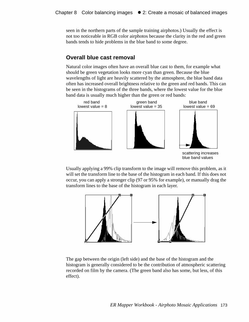
Chapter 8#Color balancing images#z 2: Create a mosaic of balanced images
t is reen
at
ata is can blue
s it s not the
ring this
seen in the northern parts of the sample training airphotos.) Usually the effecnot too noticeable in RGB color airphotos because the clarity in the red and gbands tends to hide problems in the blue band to some degree.
Overall blue cast removal
Natural color images often have an overall blue cast to them, for example whshould be green vegetation looks more cyan than green. Because the blue wavelengths of light are heavily scattered by the atmosphere, the blue band doften has increased overall brightness relative to the green and red bands. Thbe seen in the histograms of the three bands, where the lowest value for the band data is usually much higher than the green or red bands:
Usually applying a 99% clip transform to the image will remove this problem, awill set the transform line to the base of the histogram in each band. If this doeoccur, you can apply a stronger clip (97 or 95% for example), or manually dragtransform lines to the base of the histogram in each layer.
The gap between the origin (left side) and the base of the histogram and the histogram is generally considered to be the contribution of atmospheric scatterecorded on film by the camera. (The green band also has some, but less, ofeffect).
red band green band blue band
scattering increasesblue band values
lowest value = 69lowest value = 35lowest value = 8
ER Mapper Workbook - Airphoto Mosaic Applications 173
Chapter 8#Color balancing images#z 2: Create a mosaic of balanced images
op black
the o
sible
st.
mula
lor ula.
, rea
Tip: Applying a 99% clip transform to the data works best if you first zoom in to croff any black edges that may have been scanned as part of the airphoto. Theedges tend to contain low or zero data values that will not be clipped off if processed as part of the image data.
Blue vignetting removal
Sometimes the blue cast or tint increases toward the edges of the image, andinterior portions look normal (a vignetting effect). Following is one way to try tremove the blue cast from only the affected areas.
1 Define and name a region polygon within the image that contains the “normal” color you expect to see (without the blue cast).
This is typically near the center of the image. Make the region as large as poswithout including any areas with a noticeable blue cast. You will use the characteristics of this area to help correct other areas affected by the blue ca
Note: Chapter 8 contains information about defining regions and using them in a foras you are asked to do here.
2 Select Cell Coordinate from the View menu.
The Cell Coordinate dialog opens.
3 In the image, click inside the region you defined and note the cell location of the area with the best “normal” RGB color in Dataset X,Y coordinates.
You are looking for the location (within the overall region) of the best overall cobalance in the image. You will use this X,Y cell location in the correction form
4 Select the Blue layer in your algorithm, then click the Edit Formula button in the process diagram.
5 Load the formula ‘anti_vignetting.frm’ in the ‘mosaic’ directory.
6 Edit the formula text to add the following before the it (where <formula> is the existing anti vignette formula):
IF INREGION(REGION1) THEN INPUT1 ELSE <formula>
This formula tells ER Mapper that “if the data falls inside the good area regionthen display it without changes, else apply the antivignetting formula (to the aoutside the region).”
7 In the Formula dialog, click on the ‘Regions’ option button, then select your good region name from the ‘REGION1’ drop-down list.
174 ER Mapper Workbook - Airphoto Mosaic Applications
Chapter 8#Color balancing images#z 2: Create a mosaic of balanced images
o
ft se
ove se
0 but
8 In the Formula dialog, click on the ‘Variables’ option button, then set the variables to the following values:
OFFSET- a factor controlling the amount of offset to the blue histogram (set tzero for now, you will adjust this later).
X_Center - the X (column) cell location of the “good color” area in dataset X,Ycoordinates (from step 3)
Y_Center - the Y (row) cell location of the “good color” area in dataset X,Y coordinates (from step 3)
X_Factor - a factor controlling the amount of blue color adjustment in areas leand right of the good region; suggested values are 0.1 to 0.35. (Try one of thevalues, you will need to experiment to get it right.)
Y_Factor - a factor controlling the amount of blue color adjustment in areas aband below the good region; suggested values are 0.1 to 0.35. (Try one of thevalues, you will need to experiment to get it right.)
The entire image should appear with a slight blue cast.
9 Click the Edit Transform Limits button in the process diagram, then analyze the blue band histogram.
The histogram should have two peaks, one representing the “good” area andanother (to the right) representing the area affected by the blue cast. Note thedifference in data values between the two peaks (usually this is about 60 to 8varies with each image). This is the value for the OFFSET variable.
10 Enter the valued determined in step 10 for the ‘OFFSET’ variable in the Formula dialog.
11 Continue to adjust the OFFSET, X_Factor and Y_Factor variables until the image has a constant blue cast across it (no noticeable color shift).
12 Finally, adjust the transforms for the red and green layers until the entire image appears in the “normal” RGB color you want.
ER Mapper Workbook - Airphoto Mosaic Applications 175

Chapter 8#Color balancing images#z 2: Create a mosaic of balanced images
176 ER Mapper Workbook - Airphoto Mosaic Applications
eams create
f the
s and
n along best e a
9
Removing seamlines
This chapter explains techniques you can use to minimize or remove visible sbetween images in a mosaic. This may not always be necessary, but it helps a “seamless” final mosaic.
Note: The Color Balancing Wizard will do all that is described in this chapter automatically. These descriptions are included to give you an understanding oprocesses involved.
About regions and featheringAfter the previous exercise, you have learned to correct the overall brightnescontrast problems encountered in creating mosaics. This is the first step in balancing the overall contrast of the mosaic to help create one continuous, seamless image. However, there are always minor contrast problems betweeadjacent images that cannot be removed, and slight mismatches of features seam lines due to slight errors in the rectification of the images. To create thepossible mosaic, ER Mapper has two additional features that help you achievfinal “seamless” look. They are:
• region polygons to constrain the overlap between images to exact areas
ER Mapper Workbook - Airphoto Mosaic Applications 177
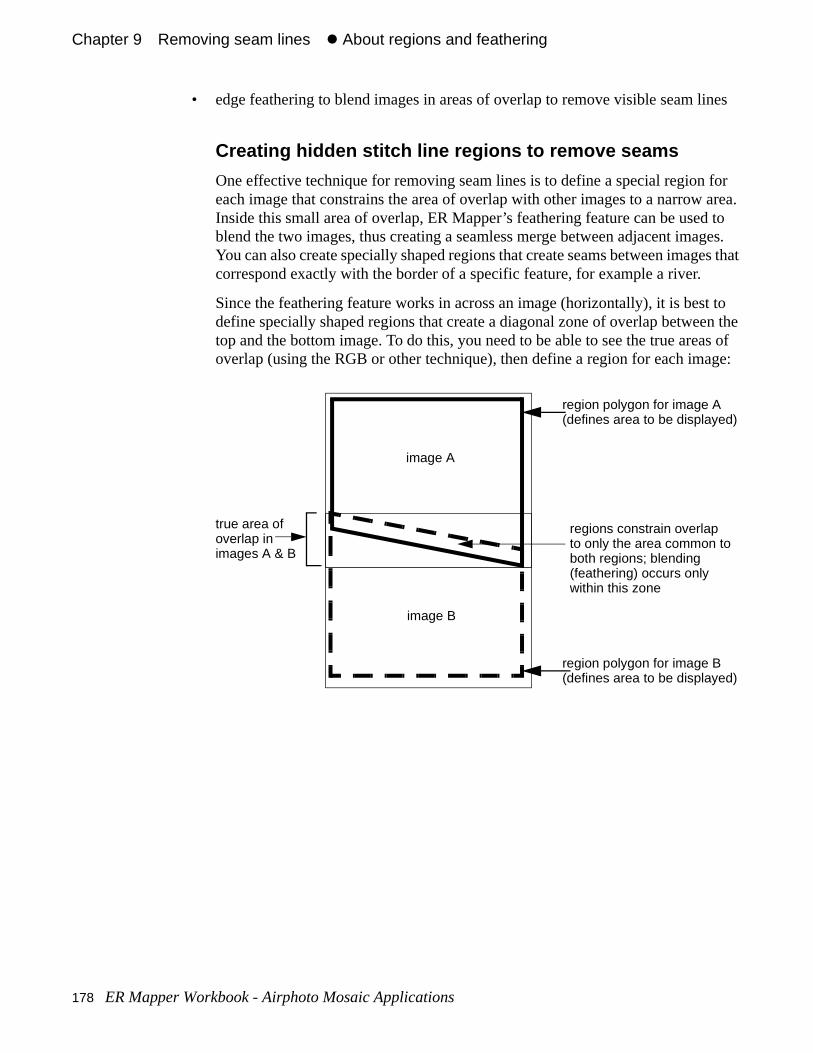
Chapter 9#Removing seam lines#z About regions and feathering
ines
for area. to ges. es that
t to en the as of ge:
• edge feathering to blend images in areas of overlap to remove visible seam l
Creating hidden stitch line regions to remove seams
One effective technique for removing seam lines is to define a special regioneach image that constrains the area of overlap with other images to a narrowInside this small area of overlap, ER Mapper’s feathering feature can be usedblend the two images, thus creating a seamless merge between adjacent imaYou can also create specially shaped regions that create seams between imagcorrespond exactly with the border of a specific feature, for example a river.
Since the feathering feature works in across an image (horizontally), it is besdefine specially shaped regions that create a diagonal zone of overlap betwetop and the bottom image. To do this, you need to be able to see the true areoverlap (using the RGB or other technique), then define a region for each ima
image A
image B
region polygon for image A(defines area to be displayed)
region polygon for image B(defines area to be displayed)
true area ofoverlap inimages A & B
regions constrain overlapto only the area common toboth regions; blending(feathering) occurs onlywithin this zone
178 ER Mapper Workbook - Airphoto Mosaic Applications
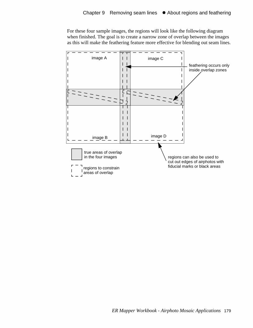
Chapter 9#Removing seam lines#z About regions and feathering
ages
lines.
For these four sample images, the regions will look like the following diagramwhen finished. The goal is to create a narrow zone of overlap between the imas this will make the feathering feature more effective for blending out seam
image A
image B
feathering occurs onlyinside overlap zones
image D
image C
true areas of overlapin the four images
regions to constrainareas of overlap
regions can also be used tocut out edges of airphotos withfiducial marks or black areas
ER Mapper Workbook - Airphoto Mosaic Applications 179
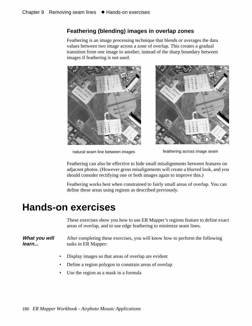
Chapter 9#Removing seam lines#z Hands-on exercises
a
s on you
can
exact
Feathering (blending) images in overlap zones
Feathering is an image processing technique that blends or averages the datvalues between two image across a zone of overlap. This creates a gradual transition from one image to another, instead of the sharp boundary betweenimages if feathering is not used.
Feathering can also be effective to hide small misalignments between featureadjacent photos. (However gross misalignments will create a blurred look, andshould consider rectifying one or both images again to improve this.)
Feathering works best when constrained to fairly small areas of overlap. You define these areas using regions as described previously.
Hands-on exercisesThese exercises show you how to use ER Mapper’s regions feature to defineareas of overlap, and to use edge feathering to minimize seam lines.
• Display images so that areas of overlap are evident
• Define a region polygon to constrain areas of overlap
• Use the region as a mask in a formula
What you will learn...
After completing these exercises, you will know how to perform the following tasks in ER Mapper:
natural seam line between images feathering across image seam
180 ER Mapper Workbook - Airphoto Mosaic Applications
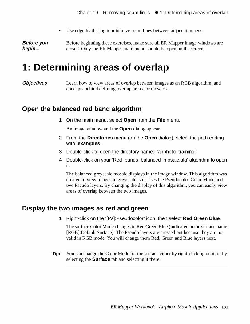
Chapter 9#Removing seam lines#z 1: Determining areas of overlap
was and view
name not
r by
are
nd
• Use edge feathering to minimize seam lines between adjacent images
1: Determining areas of overlap
Open the balanced red band algorithm
1 On the main menu, select Open from the File menu.
An image window and the Open dialog appear.
2 From the Directories menu (on the Open dialog), select the path ending with \examples .
3 Double-click to open the directory named ‘airphoto_training.’
4 Double-click on your ‘Red_bands_balanced_mosaic.alg’ algorithm to open it.
The balanced greyscale mosaic displays in the image window. This algorithmcreated to view images in greyscale, so it uses the Pseudocolor Color Mode two Pseudo layers. By changing the display of this algorithm, you can easily areas of overlap between the two images.
Display the two images as red and green1 Right-click on the ‘[Ps]:Pseudocolor’ icon, then select Red Green Blue .
The surface Color Mode changes to Red Green Blue (indicated in the surface[RGB]:Default Surface). The Pseudo layers are crossed out because they arevalid in RGB mode. You will change them Red, Green and Blue layers next.
Tip: You can change the Color Mode for the surface either by right-clicking on it, oselecting the Surface tab and selecting it there.
Before you begin...
Before beginning these exercises, make sure all ER Mapper image windows closed. Only the ER Mapper main menu should be open on the screen.
Objectives Learn how to view areas of overlap between images as an RGB algorithm, aconcepts behind defining overlap areas for mosaics.
ER Mapper Workbook - Airphoto Mosaic Applications 181
Chapter 9#Removing seam lines#z 1: Determining areas of overlap
reas en . een r
ween e t
ly d
me not
e the h a in the
2 Right-click on each of the two layers and change them to Red and Green layers as shown below:
The mosaic redisplays so each of the images is shown in a different color . Aof overlap are clearly visible by the color that results from mixing red and greThe area of overlap between the images is shown in yellow (since red and grcombine to create yellow). Areas where images do not overlap are shown as eithered or green.
Tip: This technique is also a good way to evaluate the accuracy of registration bettwo images in the area of overlap. For example, where a red and green imagoverlap, you will typically see a red or green “halo” around features that do noalign well in the two images. (This is caused by the same feature being slightoffset in the two images.) Good registration will make features appear as soliyellow.
Display the images as a greyscale mosaic again1 Right-click on the ‘[RGB]:Pseudocolor’ icon, then select Pseudocolor .
The surface Color Mode changes to Pseudocolor (indicated in the surface na[Ps]:Default Surface). The Red and Green are crossed out because they are valid in Pseudocolor mode.
2 Right-click on each of the two layers and change them to Pseudo layers:
The mosaic redisplays in greyscale again. As you can see, it is easy to changtype of display and color mode for an algorithm as needed to help accomplisparticular task. (In this case, you wanted to see the overlap between images mosaic.)
Change to Red
Change to Green
182 ER Mapper Workbook - Airphoto Mosaic Applications
Chapter 9#Removing seam lines#z 2: Defining regions to constrain overlap
or
ed
n d to
lap.
2: Defining regions to constrain overlap
You will learn the method used to actually define and name region polygons fthe raster datasets in the mosaic.
Add a vector layer for region definition to the first dataset1 In the Algorithm dialog, right-click on the lower layer and select Turn Off .
The ‘San_Diego_Airphoto_34_rectified.ers’ image will be the only one to be displayed.
2 On the main menu (or Algorithm dialog), click the Annotate Vector Layer
button.
The New Map Composition dialog box opens.
3 Select the ‘Raster Region’ option button, then click OK.
The Raster Region option tells ER Mapper that the annotation layer will be usto create regions for a raster dataset.
ER Mapper opens the Tools palette dialog box containing your vector annotatiotools. Also notice that a new vector layer titled ‘Region Layer’ has been addethe layer list in the Algorithm window.
Define and name a region polygon
1 On the Tools palette dialog, click on the Polygon button.
2 Draw a polygon on the by clicking once at each point, then double-clicking to close the polygon. (Make your polygon fairly large.) The polygon should
Objectives Learn how to define region polygons, how to view areas of overlap between images, and how to reference regions in a formula to constrain areas of overAlso learn the concepts behind defining overlap areas for mosaics.
ER Mapper Workbook - Airphoto Mosaic Applications 183
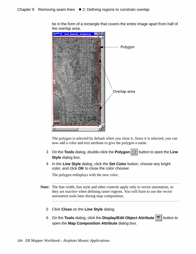
Chapter 9#Removing seam lines#z 2: Defining regions to constrain overlap
can
o r
be in the form of a rectangle that covers the entire image apart from half of the overlap area.
The polygon is selected by default when you close it. Since it is selected, younow add a color and text attribute to give the polygon a name.
3 On the Tools dialog, double-click the Polygon button to open the Line Style dialog box.
4 In the Line Style dialog, click the Set Color button, choose any bright color, and click OK to close the color chooser.
The polygon redisplays with the new color.
Note: The line width, line style and other controls apply only to vector annotation, sthey are inactive when defining raster regions. You will learn to use the vectoannotation tools later during map composition.
5 Click Close on the Line Style dialog.
6 On the Tools dialog, click the Display/Edit Object Attribute button to open the Map Composition Attribute dialog box.
Polygon
Overlap area
184 ER Mapper Workbook - Airphoto Mosaic Applications
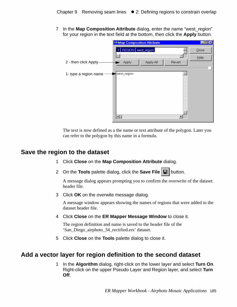
Chapter 9#Removing seam lines#z 2: Defining regions to constrain overlap
ou
set
to the
7 In the Map Composition Attribute dialog, enter the name “west_region” for your region in the text field at the bottom, then click the Apply button.
The text is now defined as a the name or text attribute of the polygon. Later ycan refer to the polygon by this name in a formula.
Save the region to the dataset1 Click Close on the Map Composition Attribute dialog.
2 On the Tools palette dialog, click the Save File button.
A message dialog appears prompting you to confirm the overwrite of the dataheader file.
3 Click OK on the overwite message dialog.
A message window appears showing the names of regions that were added dataset header file.
4 Click Close on the ER Mapper Message Window to close it.
The region definition and name is saved to the header file of the ‘San_Diego_airphoto_34_rectified.ers’ dataset.
5 Click Close on the Tools palette dialog to close it.
Add a vector layer for region definition to the second dataset1 In the Algorithm dialog, right-click on the lower layer and select Turn On .
Right-click on the upper Pseudo Layer and Region layer, and select Turn Off .
1- type a region name
2 - then click Apply
ER Mapper Workbook - Airphoto Mosaic Applications 185
Chapter 9#Removing seam lines#z 2: Defining regions to constrain overlap
ed
n d to
can
o r
The ‘San_Diego_Airphoto_36_rectified.ers’ image will be the only one to be displayed.
2 On the main menu (or Algorithm dialog), click the Annotate Vector Layer
button.
The New Map Composition dialog box opens.
3 Select the ‘Raster Region’ option button, then click OK.
The Raster Region option tells ER Mapper that the annotation layer will be usto create regions for a raster dataset.
ER Mapper opens the Tools palette dialog box containing your vector annotatiotools. Also notice that a new vector layer titled ‘Region Layer’ has been addethe layer list in the Algorithm window.
Define and name a region polygon
1 On the Tools palette dialog, click on the Polygon button.
2 Draw a polygon on the by clicking once at each point, then double-clicking to close the polygon. (Make your polygon fairly large.) The polygon should be in the form of a rectangle that covers the entire image apart from half of the overlap area.
The polygon is selected by default when you close it. Since it is selected, younow add a color and text attribute to give the polygon a name.
3 On the Tools dialog, double-click the Polygon button to open the Line Style dialog box.
4 In the Line Style dialog, click the Set Color button, choose a different bright color, and click OK to close the color chooser.
The polygon redisplays with the new color.
Note: The line width, line style and other controls apply only to vector annotation, sthey are inactive when defining raster regions. You will learn to use the vectoannotation tools later during map composition.
5 Click Close on the Line Style dialog.
6 On the Tools dialog, click the Display/Edit Object Attribute button to open the Map Composition Attribute dialog box.
186 ER Mapper Workbook - Airphoto Mosaic Applications
Chapter 9#Removing seam lines#z 2: Defining regions to constrain overlap
ou
set
to the
ion
yed
7 In the Map Composition Attribute dialog, enter the name “east_region” for your region in the text field at the bottom, then click the Apply button.
The text is now defined as a the name or text attribute of the polygon. Later ycan refer to the polygon by this name in a formula.
Save the region to the dataset1 Click Close on the Map Composition Attribute dialog.
2 On the Tools palette dialog, click the Save File button.
A message dialog appears prompting you to confirm the overwrite of the dataheader file.
3 Click OK on the overwite message dialog.
A message window appears showing the names of regions that were added dataset header file.
4 Click Close on the ER Mapper Message Window to close it.
The region definition and name is saved to the header file of the ‘San_Diego_airphoto_36_rectified.ers’ dataset.
5 Click Close on the Tools palette dialog to close it.
Display the region polygons over the image mosaicEach one of the four sample airphoto images already has an appropriate regpolygon defined to constrain the areas of overlap. Now you will learn how to display the regions simultaneously for all images in the mosaic.
1 In the Algorithm dialog, turn on all the layers by right-clicking on them and selecting Turn on .
The two Pseudo and their corresponding Region layers should now be displa
ER Mapper Workbook - Airphoto Mosaic Applications 187
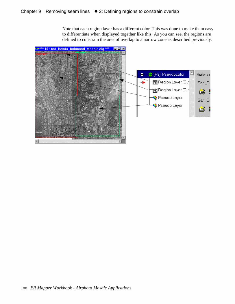
Chapter 9#Removing seam lines#z 2: Defining regions to constrain overlap
easy are usly.
Note that each region layer has a different color. This was done to make themto differentiate when displayed together like this. As you can see, the regionsdefined to constrain the area of overlap to a narrow zone as described previo
188 ER Mapper Workbook - Airphoto Mosaic Applications
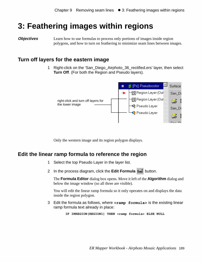
Chapter 9#Removing seam lines#z 3: Feathering images within regions
ata
ges.
3: Feathering images within regions
Turn off layers for the eastern image1 Right-click on the ‘San_Diego_Airphoto_36_rectified.ers’ layer, then select
Turn Off . (For both the Region and Pseudo layers).
Only the western image and its region polygon displays.
Edit the linear ramp formula to reference the region1 Select the top Pseudo Layer in the layer list.
2 In the process diagram, click the Edit Formula button.
The Formula Editor dialog box opens. Move it left of the Algorithm dialog and below the image window (so all three are visible).
You will edit the linear ramp formula so it only operates on and displays the dinside the region polygon.
3 Edit the formula as follows, where <ramp formula> is the existing linear ramp formula text already in place:
IF INREGION(REGION1) THEN <ramp formula> ELSE NULL
Objectives Learn how to use formulas to process only portions of images inside region polygons, and how to turn on feathering to minimize seam lines between ima
right-click and turn off layers forthe lower image
ER Mapper Workbook - Airphoto Mosaic Applications 189
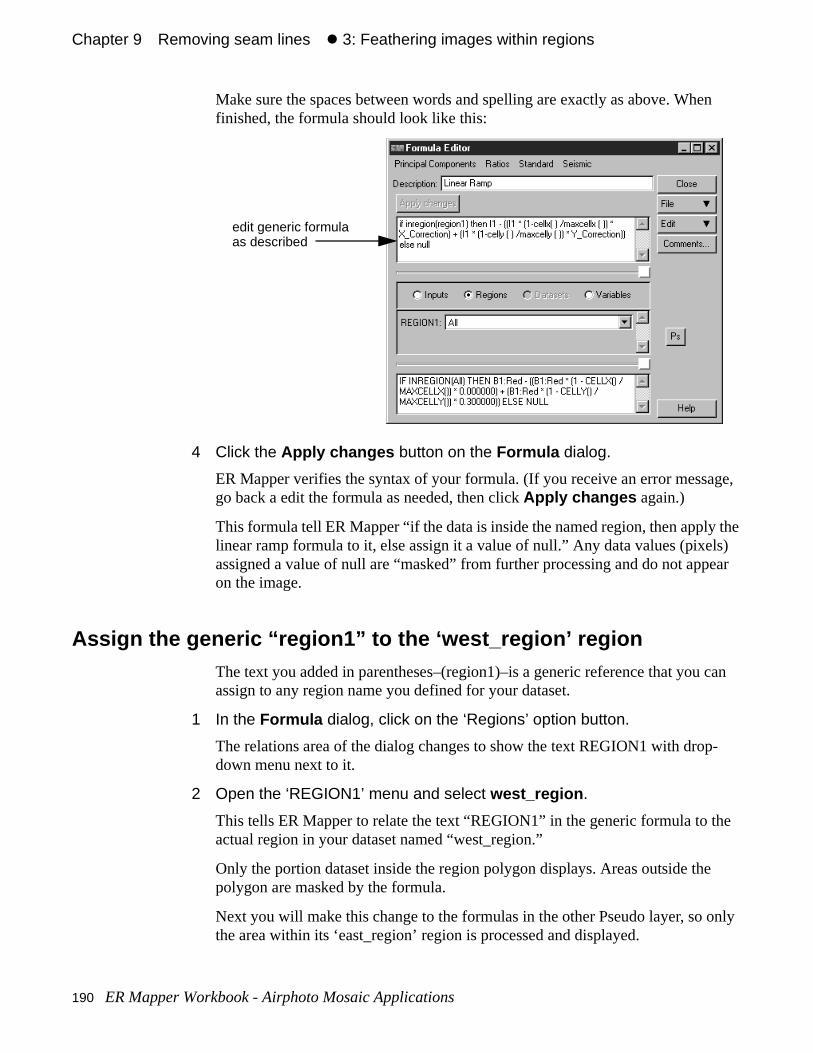
Chapter 9#Removing seam lines#z 3: Feathering images within regions
en
ge,
the s) ear
can
-
e
only
Make sure the spaces between words and spelling are exactly as above. Whfinished, the formula should look like this:
4 Click the Apply changes button on the Formula dialog.
ER Mapper verifies the syntax of your formula. (If you receive an error messago back a edit the formula as needed, then click Apply changes again.)
This formula tell ER Mapper “if the data is inside the named region, then applylinear ramp formula to it, else assign it a value of null.” Any data values (pixelassigned a value of null are “masked” from further processing and do not appon the image.
Assign the generic “region1” to the ‘west_region’ regionThe text you added in parentheses–(region1)–is a generic reference that youassign to any region name you defined for your dataset.
1 In the Formula dialog, click on the ‘Regions’ option button.
The relations area of the dialog changes to show the text REGION1 with dropdown menu next to it.
2 Open the ‘REGION1’ menu and select west_region .
This tells ER Mapper to relate the text “REGION1” in the generic formula to thactual region in your dataset named “west_region.”
Only the portion dataset inside the region polygon displays. Areas outside thepolygon are masked by the formula.
Next you will make this change to the formulas in the other Pseudo layer, so the area within its ‘east_region’ region is processed and displayed.
edit generic formulaas described
190 ER Mapper Workbook - Airphoto Mosaic Applications
Chapter 9#Removing seam lines#z 3: Feathering images within regions
cut is out
r ng
Save the modified linear ramp formulaSince you want to add the same formula to the other Pseudo layer, one shortto save the formula. That way, you can load it directly into the other layer withhaving to retype the text.
1 From the File menu (on the Formula dialog), select Save As .
The Save Formula file chooser dialog opens. It is already set to the directorycontaining the original ‘linear_ramp.frm’ formula, and you will save your modified version in the same place.
2 In the Save As field, enter the text linear_ramp_inregion then click OK.
Your formula is now saved to disk and can be reloaded at any time.
Turn on all layers in the algorithm1 Right-click on both the layers for the lower dataset, then select Turn On .
(For both the Region and Pseudo layer)
Add the inregion formula to the other Pseudo layer1 Select the second Pseudo layer in the algorithm.
The contents of its formula appear in the Formula dialog box, the default linearamp formula without the region statement. (This should be the layer containithe ‘SE_photo’ dataset.)
2 On the Formula dialog, select Open from the File menu.
The Open Formula file chooser dialog opens. It is already set to the directorycontaining both the original ‘linear_ramp.frm’ formula and your modified ‘linear_ramp_inregion.frm’ version.
3 Click on your ‘linear_ramp_inregion.frm’ formula, then click OK.
The formula is loaded and replaces the original linear ramp formula.
Your modified formula is now loaded into both Pseudo layers, so it will both images.
4 Click Close on the Formula dialog to close it.
Display the images as red and green1 Right-click on the ‘[Ps]:Pseudocolor’ surface icon, then select Red Green
Blue .
ER Mapper Workbook - Airphoto Mosaic Applications 191
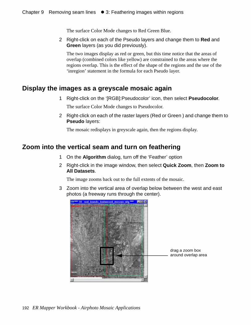
Chapter 9#Removing seam lines#z 3: Feathering images within regions
he
The surface Color Mode changes to Red Green Blue.
2 Right-click on each of the Pseudo layers and change them to Red and Green layers (as you did previously).
The two images display as red or green, but this time notice that the areas ofoverlap (combined colors like yellow) are constrained to the areas where the regions overlap. This is the effect of the shape of the regions and the use of t‘inregion’ statement in the formula for each Pseudo layer.
Display the images as a greyscale mosaic again1 Right-click on the ‘[RGB]:Pseudocolor’ icon, then select Pseudocolor .
The surface Color Mode changes to Pseudocolor.
2 Right-click on each of the raster layers (Red or Green ) and change them to Pseudo layers:
The mosaic redisplays in greyscale again, then the regions display.
Zoom into the vertical seam and turn on feathering1 On the Algorithm dialog, turn off the ‘Feather’ option
2 Right-click in the image window, then select Quick Zoom , then Zoom to All Datasets .
The image zooms back out to the full extents of the mosaic.
3 Zoom into the vertical area of overlap below between the west and east photos (a freeway runs through the center).
drag a zoom boxaround overlap area
192 ER Mapper Workbook - Airphoto Mosaic Applications
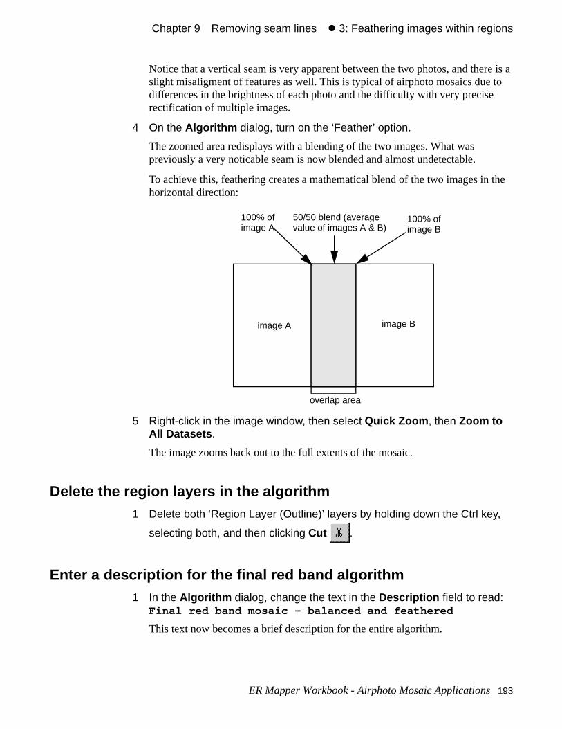
Chapter 9#Removing seam lines#z 3: Feathering images within regions
re is a to
the
Notice that a vertical seam is very apparent between the two photos, and theslight misaligment of features as well. This is typical of airphoto mosaics due differences in the brightness of each photo and the difficulty with very preciserectification of multiple images.
4 On the Algorithm dialog, turn on the ‘Feather’ option.
The zoomed area redisplays with a blending of the two images. What was previously a very noticable seam is now blended and almost undetectable.
To achieve this, feathering creates a mathematical blend of the two images inhorizontal direction:
5 Right-click in the image window, then select Quick Zoom , then Zoom to All Datasets .
The image zooms back out to the full extents of the mosaic.
Delete the region layers in the algorithm1 Delete both ‘Region Layer (Outline)’ layers by holding down the Ctrl key,
selecting both, and then clicking Cut .
Enter a description for the final red band algorithm1 In the Algorithm dialog, change the text in the Description field to read:
Final red band mosaic - balanced and feathered
This text now becomes a brief description for the entire algorithm.
overlap area
image A image B
100% ofimage A
100% ofimage B
50/50 blend (averagevalue of images A & B)
ER Mapper Workbook - Airphoto Mosaic Applications 193
Chapter 9#Removing seam lines#z 3: Feathering images within regions
green
s
Save the final red band algorithm to disk1 From the File menu (on the main menu), select Save As... .
The Save As... file chooser dialog opens.
2 In the Files of Type: field, select ‘ER Mapper Algorithm (.alg)’
3 In the Save As: text field, type the following filename:
Final_red_bands_mosaic
This name denotes that it is the final mosaic of the red band images.
4 Click OK to save the algorithm.
Your final red band algorithm is now saved to an algorithm file on disk.
The next step is would be to create balanced and feathered algorithms for theand blue band images, then assemble them into a final RGB color mosaic.
Close the image window and Algorithm dialog1 Close the image window by selecting Close from the File menu.
2 Click Close on the Algorithm dialog to close it.
Only the ER Mapper main menu should be open on the screen.
• Define a region polygon to constrain areas of overlap
• Display images so that areas of overlap are evident
• Use the the region as a mask in a formula
• Use edge feathering to minimize seam lines between adjacent images
What you learned
After completing these exercises, you know how to perform the following taskin ER Mapper:
194 ER Mapper Workbook - Airphoto Mosaic Applications
een e
e
er
s. For lor
10
Creating the finalmosaic
This chapter explains how to apply the same processing techniques to the grand blue band data in each image, and assemble them into a final RGB colormosaic. You will also learn about using an algorithm as a template to apply thsame processing to other bands or datasets.
Note: The information in this chapter is provided to give you an understanding of thprocesses involved. You would normally use the Color Balancing Wizard to do this automatically.
About algorithms as templatesAny algorithm can be used as a template to apply the same processing to othdatasets without having to repeat all the steps used to create the algorithm originally. This can save you much time and trouble, and simplify what can sometimes be rather complex processing to create large mosaics of airphotoexample, instead of repeating all the steps in the previous two chapters to cobalance and feather the green and blue band data, you will use the red bandalgorithm you already created and simply adjust it where needed.
ER Mapper Workbook - Airphoto Mosaic Applications 195
Chapter 10#Creating the final mosaic#z Hands-on exercises
age
lets riting
u other ess
ctly and.
rithm ions, pper
nto a
are
Using algorithms as datasets
Up until now, you have loaded raster datasets into your algorithms (actual imfiles residing on disk). ER Mapper also lets you use an algorithm as input to another algorithm, just as if the algorithm were actually a dataset. This featureyou perform processing in stages, without using the time and disk space of wa new dataset to disk at each stage.
For example, when you balanced and feathered the four red band images, yosaved it as an algorithm. This algorithm can be loaded into the red layer of anRGB algorithm (as if it were a dataset), and ER Mapper will automatically procall four of the image files as if they were merged into a single file.
Note: ER Mapper also has an extension of the algorithm concept called a Virtual Dataset (or VDS). A Virtual Dataset is a special type of algorithm that can be used exalike a real dataset for the most part, but the virtual image is computed on dem(A VDS even has an ‘.ers’ file extension like a real dataset.) One common application for a VDS is to link several files together (such as a mosaic) and reference them as if they were one file. The difference between using an algoand a Virtual Dataset is that you can calculate statistics for a VDS, define regand several other things that you cannot do with an algorithm. See the ER MaTutorial and User Guide manuals for more information.
Hands-on exercisesThese exercises show you how to apply the final balancing and feathering processing to the green and blue bands in each image, and assemble them ifinal RGB color mosaic.
• Use an algorithm as a template to apply the same processing to other data
• Create an RGB algorithm to display the final mosaic
• Enhance the overall contrast of the final mosaic
What you will learn...
After completing these exercises, you will know how to perform the following tasks in ER Mapper:
Before you begin...
Before beginning these exercises, make sure all ER Mapper image windows closed. Only the ER Mapper main menu should be open on the screen.
196 ER Mapper Workbook - Airphoto Mosaic Applications
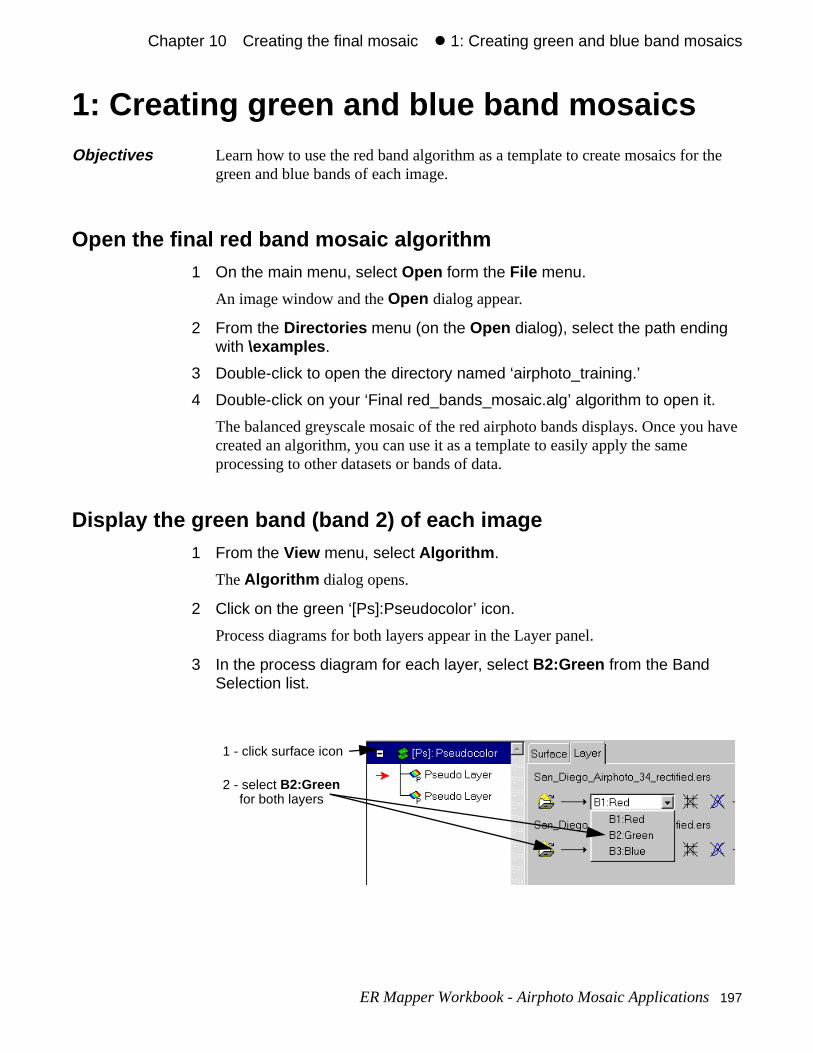
Chapter 10#Creating the final mosaic#z 1: Creating green and blue band mosaics
have
the
1: Creating green and blue band mosaics
Open the final red band mosaic algorithm1 On the main menu, select Open form the File menu.
An image window and the Open dialog appear.
2 From the Directories menu (on the Open dialog), select the path ending with \examples .
3 Double-click to open the directory named ‘airphoto_training.’
4 Double-click on your ‘Final red_bands_mosaic.alg’ algorithm to open it.
The balanced greyscale mosaic of the red airphoto bands displays. Once youcreated an algorithm, you can use it as a template to easily apply the same processing to other datasets or bands of data.
Display the green band (band 2) of each image1 From the View menu, select Algorithm .
The Algorithm dialog opens.
2 Click on the green ‘[Ps]:Pseudocolor’ icon.
Process diagrams for both layers appear in the Layer panel.
3 In the process diagram for each layer, select B2:Green from the Band Selection list.
Objectives Learn how to use the red band algorithm as a template to create mosaics forgreen and blue bands of each image.
1 - click surface icon
2 - select B2:Greenfor both layers
ER Mapper Workbook - Airphoto Mosaic Applications 197
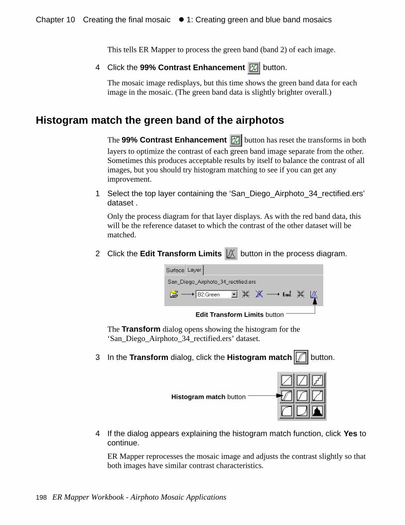
Chapter 10#Creating the final mosaic#z 1: Creating green and blue band mosaics
ch
h
ther. of all
his
o that
This tells ER Mapper to process the green band (band 2) of each image.
4 Click the 99% Contrast Enhancement button.
The mosaic image redisplays, but this time shows the green band data for eaimage in the mosaic. (The green band data is slightly brighter overall.)
Histogram match the green band of the airphotos
The 99% Contrast Enhancement button has reset the transforms in bot
layers to optimize the contrast of each green band image separate from the oSometimes this produces acceptable results by itself to balance the contrast images, but you should try histogram matching to see if you can get any improvement.
1 Select the top layer containing the ‘San_Diego_Airphoto_34_rectified.ers’ dataset .
Only the process diagram for that layer displays. As with the red band data, twill be the reference dataset to which the contrast of the other dataset will bematched.
2 Click the Edit Transform Limits button in the process diagram.
The Transform dialog opens showing the histogram for the ‘San_Diego_Airphoto_34_rectified.ers’ dataset.
3 In the Transform dialog, click the Histogram match button.
4 If the dialog appears explaining the histogram match function, click Yes to continue.
ER Mapper reprocesses the mosaic image and adjusts the contrast slightly sboth images have similar contrast characteristics.
Edit Transform Limits button
Histogram match button
198 ER Mapper Workbook - Airphoto Mosaic Applications
Chapter 10#Creating the final mosaic#z 1: Creating green and blue band mosaics
ram
is to
ou did e data ess
Tip: It is acceptable to use a different reference image for the green or blue histogmatch than for the red band. Typically, in larger mosaics, you would try other images as the reference image to see if they produce better results. The ideaget the best overall contrast between all images, no matter what manner youchoose.
5 Click Close on the Transform dialog.
You have now performed exactly the same steps on the green band data as yearlier for the red band data. Each layer has a formula that processes only thinside the region polygons, and the linear ramp formula to balance the brightnshifts across individual images.
Enter a description for the final green band algorithm1 In the Algorithm dialog, change the text in the Description field to read:
Final green band mosaic - balanced and feathered
This text now becomes a brief description for the entire algorithm.
Save the final green band algorithm to disk1 From the File menu (on the main menu), select Save As... .
The Save As... file chooser dialog opens.
2 In the Files of Type: text field, select ‘ER Mapper Algorithm (.alg)’.
3 In the Save As: text field, type the following filename:
Final_green_bands_mosaic
This name denotes that it is the final mosaic of the green band images.
4 Click OK to save the algorithm.
Your final green band algorithm is now saved to an algorithm file on disk.
Display the blue band (band 3) of each image1 From the View menu, select Algorithm .
The Algorithm dialog opens.
2 Click on the green ‘[Ps]:Pseudocolor’ icon.
Process diagrams for both layers appear in the Layer panel.
ER Mapper Workbook - Airphoto Mosaic Applications 199
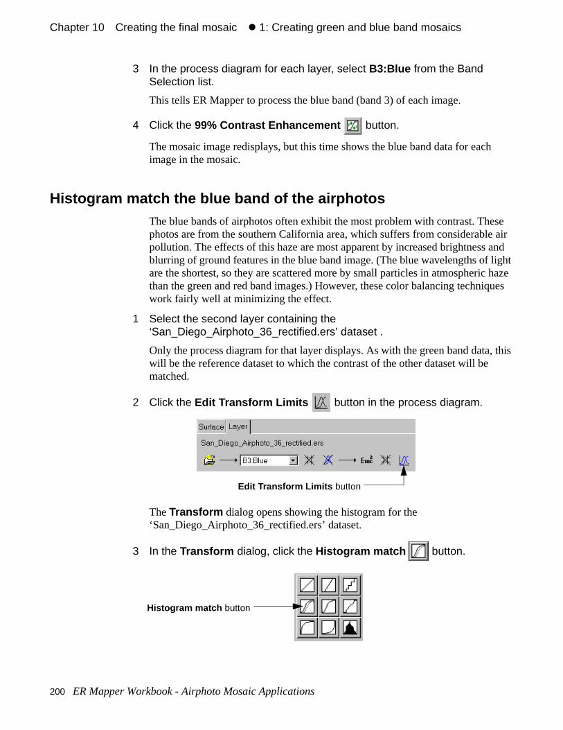
Chapter 10#Creating the final mosaic#z 1: Creating green and blue band mosaics
h
se air
and light haze ques
, this
3 In the process diagram for each layer, select B3:Blue from the Band Selection list.
This tells ER Mapper to process the blue band (band 3) of each image.
4 Click the 99% Contrast Enhancement button.
The mosaic image redisplays, but this time shows the blue band data for eacimage in the mosaic.
Histogram match the blue band of the airphotosThe blue bands of airphotos often exhibit the most problem with contrast. Thephotos are from the southern California area, which suffers from considerablepollution. The effects of this haze are most apparent by increased brightnessblurring of ground features in the blue band image. (The blue wavelengths of are the shortest, so they are scattered more by small particles in atmosphericthan the green and red band images.) However, these color balancing techniwork fairly well at minimizing the effect.
1 Select the second layer containing the ‘San_Diego_Airphoto_36_rectified.ers’ dataset .
Only the process diagram for that layer displays. As with the green band datawill be the reference dataset to which the contrast of the other dataset will bematched.
2 Click the Edit Transform Limits button in the process diagram.
The Transform dialog opens showing the histogram for the ‘San_Diego_Airphoto_36_rectified.ers’ dataset.
3 In the Transform dialog, click the Histogram match button.
Edit Transform Limits button
Histogram match button
200 ER Mapper Workbook - Airphoto Mosaic Applications

Chapter 10#Creating the final mosaic#z 2: Creating the final RGB algorithm
o that
u did
ple, red,
ow
4 If the dialog appears explaining the histogram match function, click Yes to continue.
ER Mapper reprocesses the mosaic image and adjusts the contrast slightly sall four images have similar contrast characteristics.
5 Click Close on the Transform dialog.
You have now performed exactly the same steps on the blue band data as yoearlier for the red and green bands.
Enter a description for the final blue band algorithm1 In the Algorithm dialog, change the text in the Description field to read:
Final blue band mosaic - balanced and feathered
This text now becomes a brief description for the entire algorithm.
Save the final blue band algorithm to disk1 From the File menu (on the main menu), select Save As... .
The Save As... file chooser dialog opens.
2 In the Files of Type: text field, select ‘ER Mapper Algorithm (.alg)’.
3 In the Save As: text field, type the following filename:
Final_blue_bands_mosaic
This name denotes that it is the final mosaic of the blue band images.
4 Click OK to save the algorithm.
Your final blue band algorithm is now saved to an algorithm file on disk.
2: Creating the final RGB algorithm
Run the Image Display and Mosaic WizardER Mapper lets you display an algorithm just as if it were a dataset. For examyou will take the three algorithms you created earlier and display them as thegreen and blue components of an RGB algorithm.
Objectives Learn how to display the individual band mosaics as an RGB algorithm, and hto adjust the final contrast and color.
ER Mapper Workbook - Airphoto Mosaic Applications 201
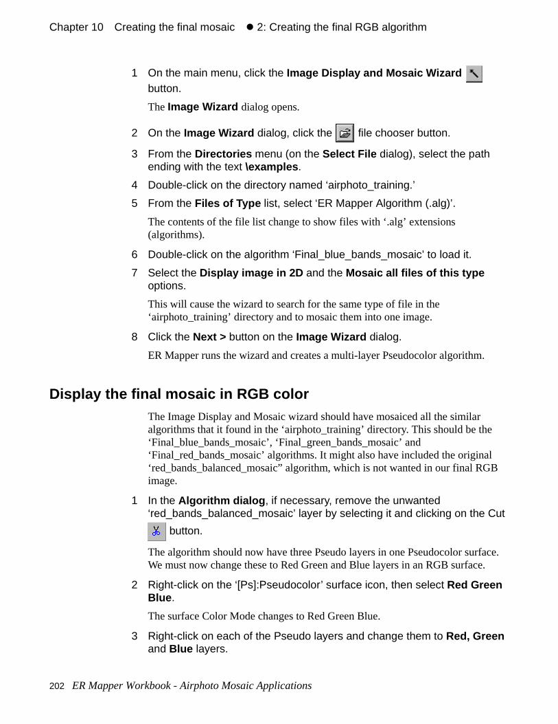
Chapter 10#Creating the final mosaic#z 2: Creating the final RGB algorithm
l B
ace. .
1 On the main menu, click the Image Display and Mosaic Wizard button.
The Image Wizard dialog opens.
2 On the Image Wizard dialog, click the file chooser button.
3 From the Directories menu (on the Select File dialog), select the path ending with the text \examples .
4 Double-click on the directory named ‘airphoto_training.’
5 From the Files of Type list, select ‘ER Mapper Algorithm (.alg)’.
The contents of the file list change to show files with ‘.alg’ extensions (algorithms).
6 Double-click on the algorithm ‘Final_blue_bands_mosaic’ to load it.
7 Select the Display image in 2D and the Mosaic all files of this type options.
This will cause the wizard to search for the same type of file in the ‘airphoto_training’ directory and to mosaic them into one image.
8 Click the Next > button on the Image Wizard dialog.
ER Mapper runs the wizard and creates a multi-layer Pseudocolor algorithm.
Display the final mosaic in RGB colorThe Image Display and Mosaic wizard should have mosaiced all the similar algorithms that it found in the ‘airphoto_training’ directory. This should be the‘Final_blue_bands_mosaic’, ‘Final_green_bands_mosaic’ and ‘Final_red_bands_mosaic’ algorithms. It might also have included the origina‘red_bands_balanced_mosaic” algorithm, which is not wanted in our final RGimage.
1 In the Algorithm dialog , if necessary, remove the unwanted ‘red_bands_balanced_mosaic’ layer by selecting it and clicking on the Cut
button.
The algorithm should now have three Pseudo layers in one Pseudocolor surfWe must now change these to Red Green and Blue layers in an RGB surface
2 Right-click on the ‘[Ps]:Pseudocolor’ surface icon, then select Red Green Blue .
The surface Color Mode changes to Red Green Blue.
3 Right-click on each of the Pseudo layers and change them to Red, Green and Blue layers.
202 ER Mapper Workbook - Airphoto Mosaic Applications
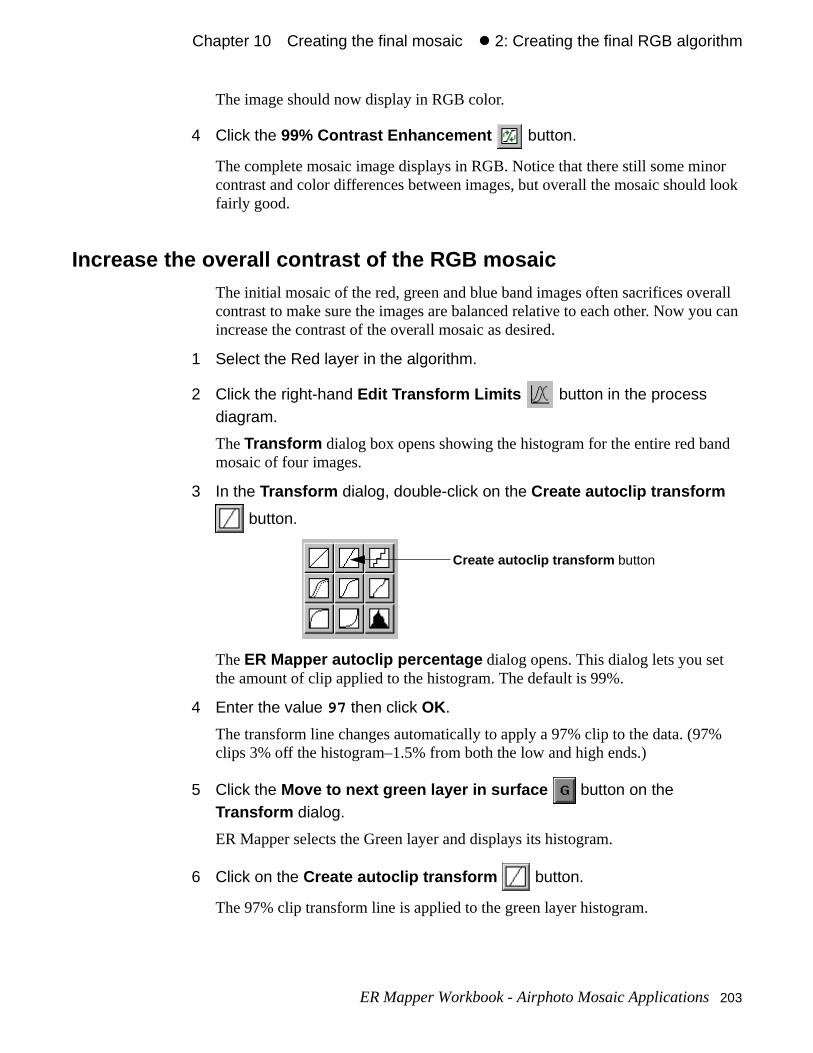
Chapter 10#Creating the final mosaic#z 2: Creating the final RGB algorithm
or look
rall u can
nd
%
The image should now display in RGB color.
4 Click the 99% Contrast Enhancement button.
The complete mosaic image displays in RGB. Notice that there still some mincontrast and color differences between images, but overall the mosaic shouldfairly good.
Increase the overall contrast of the RGB mosaicThe initial mosaic of the red, green and blue band images often sacrifices ovecontrast to make sure the images are balanced relative to each other. Now yoincrease the contrast of the overall mosaic as desired.
1 Select the Red layer in the algorithm.
2 Click the right-hand Edit Transform Limits button in the process diagram.
The Transform dialog box opens showing the histogram for the entire red bamosaic of four images.
3 In the Transform dialog, double-click on the Create autoclip transform
button.
The ER Mapper autoclip percentage dialog opens. This dialog lets you set the amount of clip applied to the histogram. The default is 99%.
4 Enter the value 97 then click OK.
The transform line changes automatically to apply a 97% clip to the data. (97clips 3% off the histogram–1.5% from both the low and high ends.)
5 Click the Move to next green layer in surface button on the Transform dialog.
ER Mapper selects the Green layer and displays its histogram.
6 Click on the Create autoclip transform button.
The 97% clip transform line is applied to the green layer histogram.
Create autoclip transform button
ER Mapper Workbook - Airphoto Mosaic Applications 203
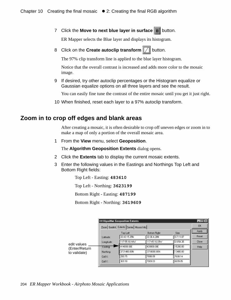
Chapter 10#Creating the final mosaic#z 2: Creating the final RGB algorithm
ic
ight.
in to
7 Click the Move to next blue layer in surface button.
ER Mapper selects the Blue layer and displays its histogram.
8 Click on the Create autoclip transform button.
The 97% clip transform line is applied to the blue layer histogram.
Notice that the overall contrast is increased and adds more color to the mosaimage.
9 If desired, try other autoclip percentages or the Histogram equalize or Gaussian equalize options on all three layers and see the result.
You can easily fine tune the contrast of the entire mosaic until you get it just r
10 When finished, reset each layer to a 97% autoclip transform.
Zoom in to crop off edges and blank areasAfter creating a mosaic, it is often desirable to crop off uneven edges or zoommake a map of only a portion of the overall mosaic area.
1 From the View menu, select Geoposition .
The Algorithm Geoposition Extents dialog opens.
2 Click the Extents tab to display the current mosaic extents.
3 Enter the following values in the Eastings and Northings Top Left and Bottom Right fields:
Top Left - Easting: 483610
Top Left - Northing: 3623199
Bottom Right - Easting: 487199
Bottom Right - Northing: 3619609
edit values(Enter/Returnto validate)
204 ER Mapper Workbook - Airphoto Mosaic Applications
Chapter 10#Creating the final mosaic#z 2: Creating the final RGB algorithm
dges ct Lat/.
s
4 Click the Apply button.
ER Mapper zooms to the exact extents you entered, which crop off the outer eof the mosaic image. You can define the image extents either by entering exaLong or E/N values, or visually by dragging a zoom box over the desired area
5 Click Close on the Algorithm Geoposition Extents dialog.
Enter a description for the final RGB algorithm1 In the Algorithm dialog, change the text in the Description field to read:
Final RGB mosaic of red/green/blue band algorithms
This text now becomes a brief description for the entire algorithm.
Save the final RGB algorithm to disk1 From the File menu (on the main menu), select Save As... .
The Save As... file chooser dialog opens.
2 In the Files of Type: field, select ‘ER Mapper Algorithm (.alg)’.
3 In the Save As: text field, type the following filename:
Final_RGB_mosaic
4 Click OK to save the algorithm.
Your final RGB algorithm is now saved to an algorithm file on disk.
Close the image windows and Algorithm dialog1 Close the image windows by selecting Close from the File menu.
2 Click Close on the Algorithm dialog to close it.
Only the ER Mapper main menu should be open on the screen.
• Use an algorithm as a template to apply the same processing to other data
• Create an RGB algorithm to display the final mosaic
• Enhance the overall contrast of the final mosaic
What you learned
After completing these exercises, you know how to perform the following taskin ER Mapper:
ER Mapper Workbook - Airphoto Mosaic Applications 205

Chapter 10#Creating the final mosaic#z 2: Creating the final RGB algorithm
206 ER Mapper Workbook - Airphoto Mosaic Applications
ive it is
s
d
saic.
11
Color balancingimage mosaicsThis chapter explains how you use the ER Mapper Image Balancing Wizard for Airphotos to balance and color match airphoto mosaics. The previous chapters outlined how you would perform these tasks manually. This was to gyou an understanding of what is involved. You will now see how much easierto use the Image Balancing Wizard for Airphotos to perform the same tasksautomatically.
Hands-on exercisesThese exercises show you how to balance and color match mosaic algorithmusing the Image Balancing Wizard for Airphotos .
For these exercises, we will be using the airphoto mosaic algorithm we createpreviously using the Image Display and Mosaic Wizard .
• Use the Image Balancing Wizard to balance and color match an airphoto mo
What you will learn...
After completing these exercises, you will know how to perform the following tasks in ER Mapper:
ER Mapper Workbook - Airphoto Mosaic Applications 207
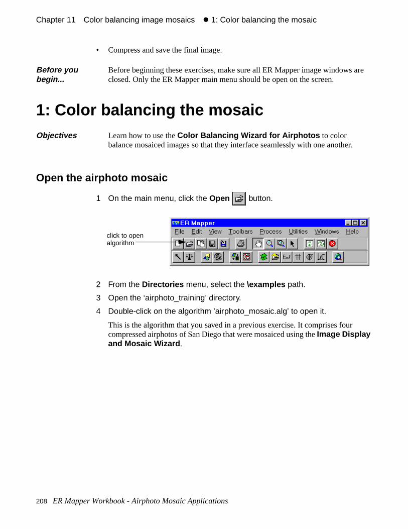
Chapter 11#Color balancing image mosaics#z 1: Color balancing the mosaic
are
.
• Compress and save the final image.
1: Color balancing the mosaic
Open the airphoto mosaic
1 On the main menu, click the Open button.
2 From the Directories menu, select the \examples path.
3 Open the ‘airphoto_training’ directory.
4 Double-click on the algorithm ’airphoto_mosaic.alg’ to open it.
This is the algorithm that you saved in a previous exercise. It comprises four compressed airphotos of San Diego that were mosaiced using the Image Display and Mosaic Wizard .
Before you begin...
Before beginning these exercises, make sure all ER Mapper image windows closed. Only the ER Mapper main menu should be open on the screen.
Objectives Learn how to use the Color Balancing Wizard for Airphotos to color balance mosaiced images so that they interface seamlessly with one another
click to openalgorithm
208 ER Mapper Workbook - Airphoto Mosaic Applications
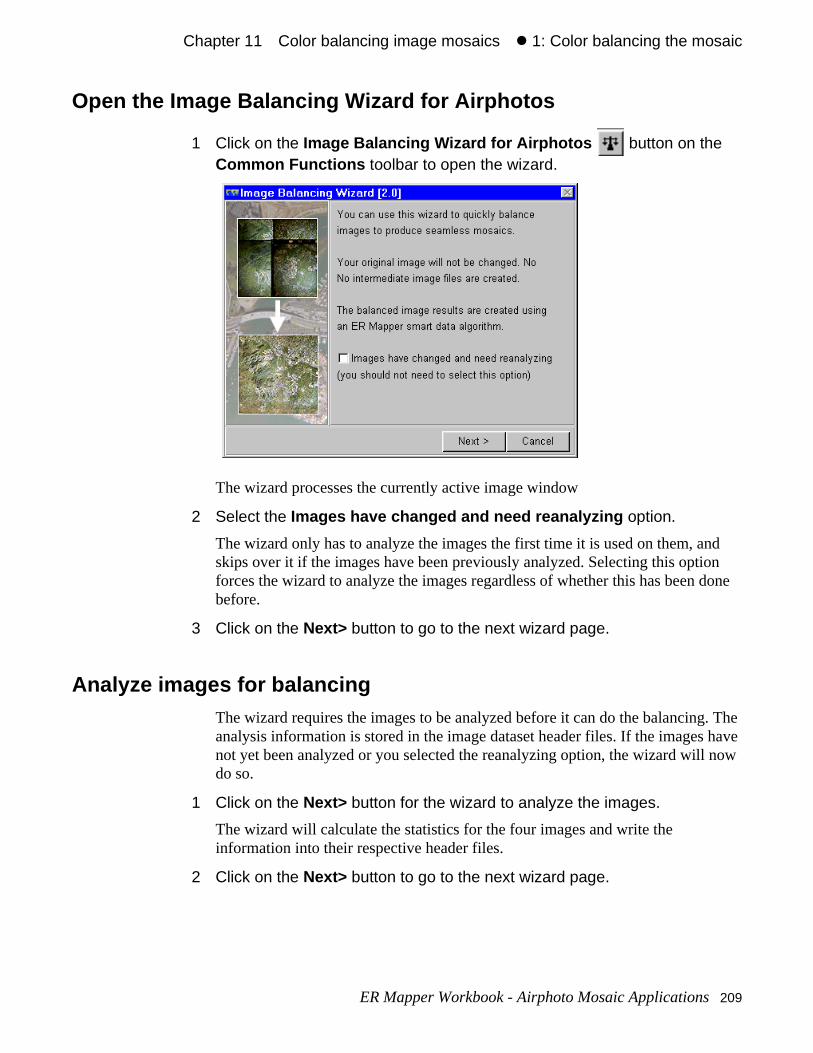
Chapter 11#Color balancing image mosaics#z 1: Color balancing the mosaic
nd n done
. The have now
Open the Image Balancing Wizard for Airphotos
1 Click on the Image Balancing Wizard for Airphotos button on the Common Functions toolbar to open the wizard.
The wizard processes the currently active image window
2 Select the Images have changed and need reanalyzing option.
The wizard only has to analyze the images the first time it is used on them, askips over it if the images have been previously analyzed. Selecting this optioforces the wizard to analyze the images regardless of whether this has been before.
3 Click on the Next> button to go to the next wizard page.
Analyze images for balancingThe wizard requires the images to be analyzed before it can do the balancinganalysis information is stored in the image dataset header files. If the imagesnot yet been analyzed or you selected the reanalyzing option, the wizard will do so.
1 Click on the Next> button for the wizard to analyze the images.
The wizard will calculate the statistics for the four images and write the information into their respective header files.
2 Click on the Next> button to go to the next wizard page.
ER Mapper Workbook - Airphoto Mosaic Applications 209
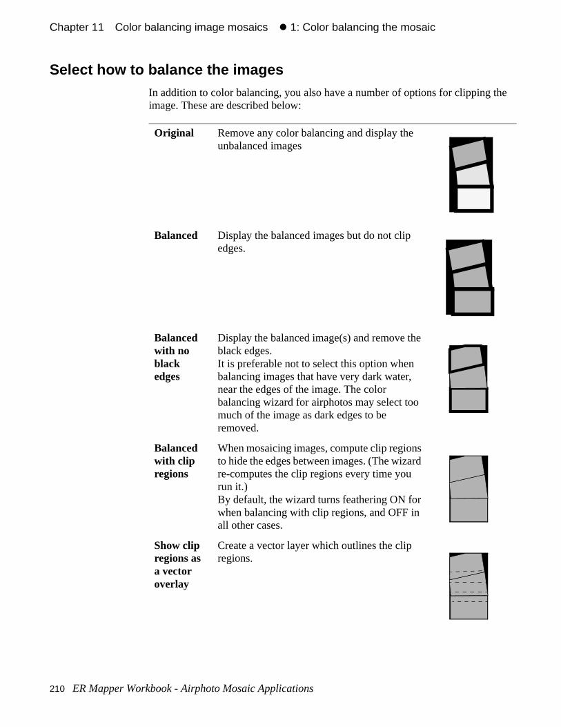
Chapter 11#Color balancing image mosaics#z 1: Color balancing the mosaic
the
Select how to balance the imagesIn addition to color balancing, you also have a number of options for clipping image. These are described below:
Original Remove any color balancing and display the unbalanced images
Balanced Display the balanced images but do not clip edges.
Balanced with no black edges
Display the balanced image(s) and remove the black edges.It is preferable not to select this option when balancing images that have very dark water, near the edges of the image. The color balancing wizard for airphotos may select too much of the image as dark edges to be removed.
Balanced with clip regions
When mosaicing images, compute clip regions to hide the edges between images. (The wizard re-computes the clip regions every time you run it.)By default, the wizard turns feathering ON for when balancing with clip regions, and OFF in all other cases.
Show clip regions as a vector overlay
Create a vector layer which outlines the clip regions.
210 ER Mapper Workbook - Airphoto Mosaic Applications
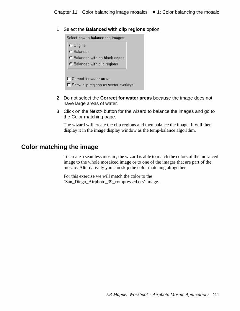
Chapter 11#Color balancing image mosaics#z 1: Color balancing the mosaic
saiced he
1 Select the Balanced with clip regions option.
2 Do not select the Correct for water areas because the image does not have large areas of water.
3 Click on the Next> button for the wizard to balance the images and go to the Color matching page.
The wizard will create the clip regions and then balance the image. It will thendisplay it in the image display window as the temp-balance algorithm.
Color matching the imageTo create a seamless mosaic, the wizard is able to match the colors of the moimage to the whole mosaiced image or to one of the images that are part of tmosaic. Alternatively you can skip the color matching altogether.
For this exercise we will match the color to the ‘San_Diego_Airphoto_39_compressed.ers’ image.
ER Mapper Workbook - Airphoto Mosaic Applications 211
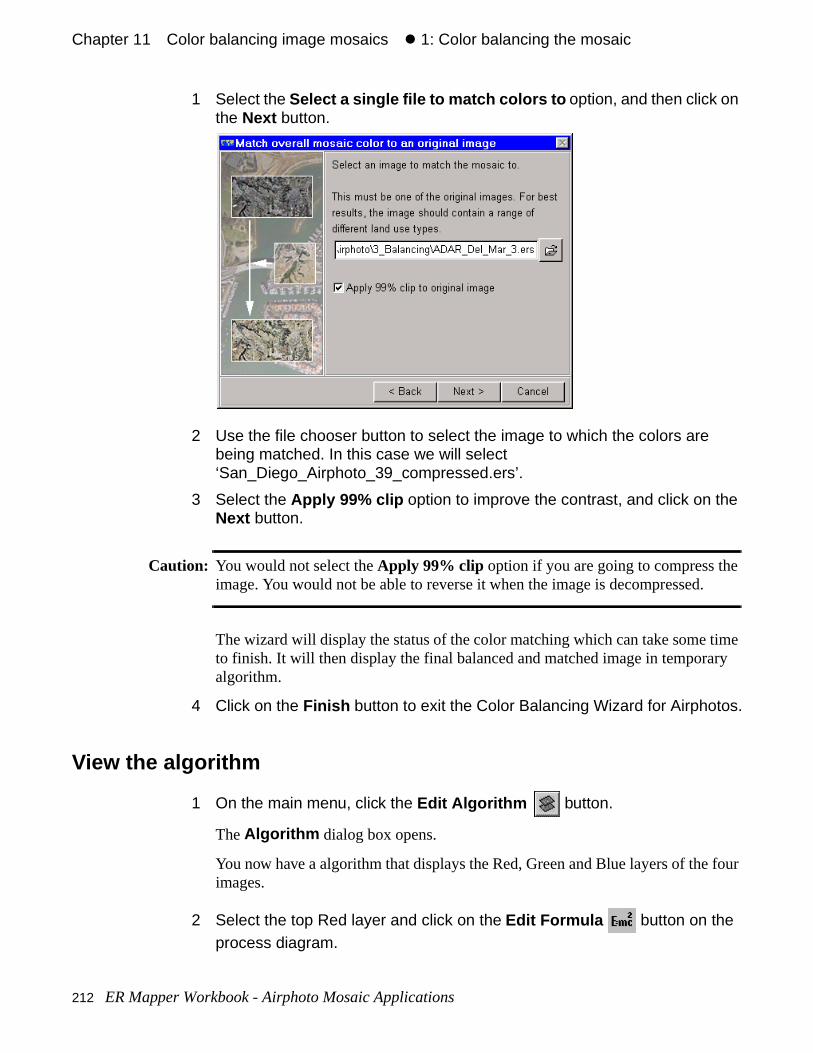
Chapter 11#Color balancing image mosaics#z 1: Color balancing the mosaic
.
time ry
four
1 Select the Select a single file to match colors to option, and then click on the Next button.
2 Use the file chooser button to select the image to which the colors are being matched. In this case we will select ‘San_Diego_Airphoto_39_compressed.ers’.
3 Select the Apply 99% clip option to improve the contrast, and click on the Next button.
Caution: You would not select the Apply 99% clip option if you are going to compress theimage. You would not be able to reverse it when the image is decompressed
The wizard will display the status of the color matching which can take some to finish. It will then display the final balanced and matched image in temporaalgorithm.
4 Click on the Finish button to exit the Color Balancing Wizard for Airphotos.
View the algorithm
1 On the main menu, click the Edit Algorithm button.
The Algorithm dialog box opens.
You now have a algorithm that displays the Red, Green and Blue layers of theimages.
2 Select the top Red layer and click on the Edit Formula button on the process diagram.
212 ER Mapper Workbook - Airphoto Mosaic Applications
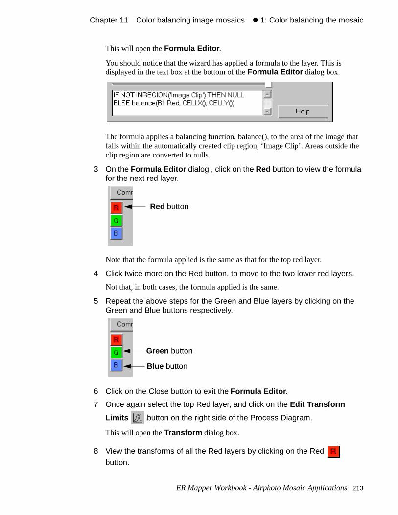
Chapter 11#Color balancing image mosaics#z 1: Color balancing the mosaic
that he
This will open the Formula Editor .
You should notice that the wizard has applied a formula to the layer. This is displayed in the text box at the bottom of the Formula Editor dialog box.
The formula applies a balancing function, balance(), to the area of the imagefalls within the automatically created clip region, ‘Image Clip’. Areas outside tclip region are converted to nulls.
3 On the Formula Editor dialog , click on the Red button to view the formula for the next red layer.
Note that the formula applied is the same as that for the top red layer.
4 Click twice more on the Red button, to move to the two lower red layers.
Not that, in both cases, the formula applied is the same.
5 Repeat the above steps for the Green and Blue layers by clicking on the Green and Blue buttons respectively.
6 Click on the Close button to exit the Formula Editor .
7 Once again select the top Red layer, and click on the Edit Transform
Limits button on the right side of the Process Diagram.
This will open the Transform dialog box.
8 View the transforms of all the Red layers by clicking on the Red button.
Red button
Green button
Blue button
ER Mapper Workbook - Airphoto Mosaic Applications 213
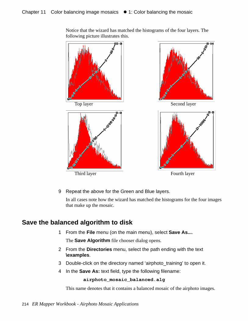
Chapter 11#Color balancing image mosaics#z 1: Color balancing the mosaic
ges
.
Notice that the wizard has matched the histograms of the four layers. The following picture illustrates this.
9 Repeat the above for the Green and Blue layers.
In all cases note how the wizard has matched the histograms for the four imathat make up the mosaic.
Save the balanced algorithm to disk1 From the File menu (on the main menu), select Save As... .
The Save Algorithm file chooser dialog opens.
2 From the Directories menu, select the path ending with the text \examples .
3 Double-click on the directory named ‘airphoto_training’ to open it.
4 In the Save As: text field, type the following filename:
airphoto_mosaic_balanced.alg
This name denotes that it contains a balanced mosaic of the airphoto images
Top layer Second layer
Third layer Fourth layer
214 ER Mapper Workbook - Airphoto Mosaic Applications
Chapter 11#Color balancing image mosaics#z 1: Color balancing the mosaic
the
s
5 Click OK to save the algorithm.
Your balanced algorithm is now saved to an algorithm file on disk.
Close the image window and Algorithm dialog1 On the main menu, select Close from the File menu to close the image
window.
2 Click Close on the Algorithm dialog.
Only the ER Mapper main menu should be open on the screen.
• Use the Color Balancing Wizard for Airphotos to balance and color matchmosaiced images.
What you learned
After completing these exercises, you know how to perform the following taskin ER Mapper:
ER Mapper Workbook - Airphoto Mosaic Applications 215

Chapter 11#Color balancing image mosaics#z 1: Color balancing the mosaic
216 ER Mapper Workbook - Airphoto Mosaic Applications
sition w to for
on the
sily on rows, ons, tor
ble. ary, e of
12
Composing mapsThis chapter explains how to use ER Mapper’s Page Setup and Map Compotools to create top quality cartographic maps. You will learn about setting up apage size, scale and extents for your map, how to draw vector annotation, hoadd map objects such as coordinate grids and scale bars, and considerationsprinting to hardcopy devices.
Note: The following exercise is a simplified example of creating a map. More detailssome aspects are provided at the end of the chapter, and you are referred to ER Mapper User Guide for more complete information.
About map compositionER Mapper provides a complete set of map composition tools that let you eatransform images into top quality image maps. Your maps can include commmap objects such as coordinate grids, scale bars, symbols, legends, north arand more. You can use the annotation tools to draw lines, text, shaded polygand other vector objects. Your maps can also include other layers to add vecdata from GIS systems, tabular data, or other external data.
ER Mapper’s map composition also has an open design and is user-extendaYou can add your own Postscript map objects to ER Mapper's map object librsuch as company logos or north arrows, include external text or graphic imagfiles, and many other types of data. You can also modify the default attributesmap objects and save them under your own unique names for later use.
ER Mapper Workbook - Airphoto Mosaic Applications 217
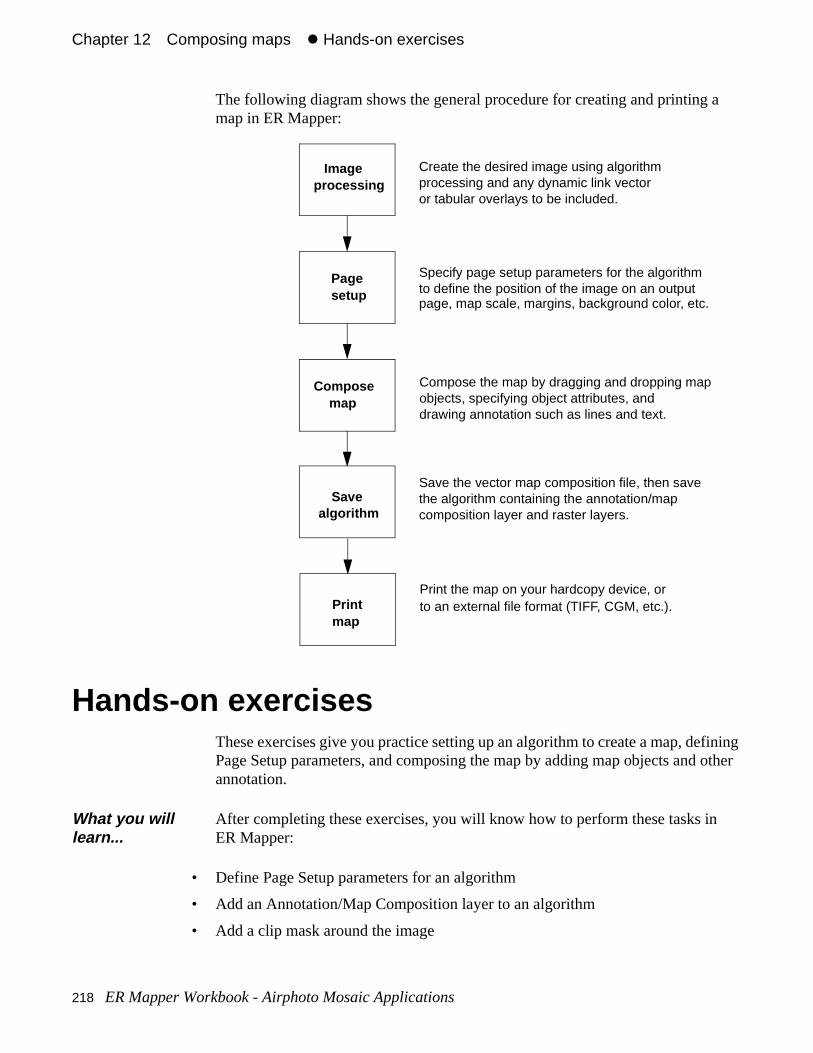
Chapter 12#Composing maps#z Hands-on exercises
a
fining other
The following diagram shows the general procedure for creating and printing map in ER Mapper:
Hands-on exercisesThese exercises give you practice setting up an algorithm to create a map, dePage Setup parameters, and composing the map by adding map objects andannotation.
• Define Page Setup parameters for an algorithm
• Add an Annotation/Map Composition layer to an algorithm
• Add a clip mask around the image
What you will learn...
After completing these exercises, you will know how to perform these tasks inER Mapper:
Image
Page
Compose
Save
Create the desired image using algorithm
Specify page setup parameters for the algorithm
Compose the map by dragging and dropping map
Save the vector map composition file, then save
processing
setup
map
processing and any dynamic link vectoror tabular overlays to be included.
to define the position of the image on an output
objects, specifying object attributes, and drawing annotation such as lines and text.
PrintPrint the map on your hardcopy device, or
mapto an external file format (TIFF, CGM, etc.).
algorithmthe algorithm containing the annotation/mapcomposition layer and raster layers.
page, map scale, margins, background color, etc.
218 ER Mapper Workbook - Airphoto Mosaic Applications
Chapter 12#Composing maps#z 1: Setting up the page
te
tions
are
age s and ted
• Draw annotation objects (lines, text, polygons, etc.) on your map
• Place map objects (grids, scale bars, etc.) on your map
• Specify color and other attributes for annotation and map objects
1: Setting up the page
Open the final RGB mosaic algorithm
1 On the main menu, click the Open button.
An image window and the Open dialog box appear.
2 From the Directories menu, select the \examples path.
3 Open the ‘airphoto_training’ directory, then double-click on the algorithm ‘airphoto_mosaic_balanced.alg’ to open it.
This is the image mosaic image you created earlier, and you will use it to creayour map.
4 Re-size the image window so that the displayed image is a perfect rectangle.
This will crop the image to remove the jagged edges.
Display the Annotation toolbar1 On the main menu, select Annotation from the Toolbars menu.
ER Mapper adds a third toolbar with buttons for quick access to common funcused for annotation and map composition.
Specify Metric or Imperial units for page setup1 On the main menu, select Preferences from the Edit menu.
Before you begin...
Before beginning these exercises, make sure all ER Mapper image windows closed. Only the ER Mapper main menu should be open on the screen.
Objectives Learn to use ER Mapper’s Page Setup options to define the position of an imon an output page, and specify other options such as map scaling parameterbackground color. In this case, you will create a 1:24,000 scale map to be prinon a large format hardcopy device.
ER Mapper Workbook - Airphoto Mosaic Applications 219
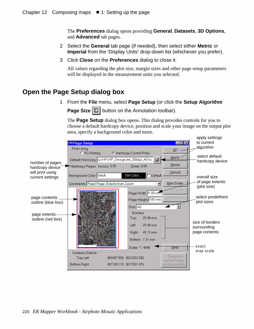
Chapter 12#Composing maps#z 1: Setting up the page
ters
t plot
The Preferences dialog opens providing General , Datasets , 3D Options , and Advanced tab pages.
2 Select the General tab page (if needed), then select either Metric or Imperial from the ‘Display Units’ drop-down list (whichever you prefer).
3 Click Close on the Preferences dialog to close it.
All values regarding the plot size, margin sizes and other page setup paramewill be displayed in the measurement units you selected.
Open the Page Setup dialog box1 From the File menu, select Page Setup (or click the Setup Algorithm
Page Size button on the Annotation toolbar).
The Page Setup dialog box opens. This dialog provides controls for you to choose a default hardcopy device, position and scale your image on the outpuarea, specify a background color and more.
page contentsoutline (blue box)
page extentsoutline (red box)
exactm ap sca le
apply settingsto currentalgorithm
overall sizeof page extents(plot size)
select predefinedplot sizes
size of borderssurroundingpage contents
select defaulthardcopy devicenumber of pages
hardcopy devicewill print usingcurrent settings
220 ER Mapper Workbook - Airphoto Mosaic Applications
Chapter 12#Composing maps#z 1: Setting up the page
on
e plot
s.
ume vice er,
d is
e cale.
Note: You can also use the Page Setup Wizard to set the page up. This will not be described in this exercise. Refer to the ER Mapper User Guide for informationthe Page Setup Wizard.
The area on the left side shows the size and shape of the plot in red (the “pagextents”), and the relative size and position of the algorithm image within the area in blue (the “contents extents”).
Select the destination hardcopy device1 Select the ‘Hardcopy Control Files’ option at the top (if it is present).
This tells ER Mapper to use its own set of device drivers. (If you are running ER Mapper on a PC, you can also choose to use the Windows drivers.)
2 Click the Default Hardcopy file chooser button.
The Default Hardcopy dialog opens to let you select the type of printer or graphics file that you will be using.
3 From the Directories menu, select the \hardcopy path.
A list of directories for categories of hardcopy devices and file formats display
4 Double-click on the directory named ‘HP’ to open it and view a list of available options for Hewlett-Packard printers.
5 Double-click on the entry ‘HP_DesignJet_300dpi_A0.hc’ to select it.
This device is now selected as your default hardcopy device, and we will assthat your example map will be printed on it. It is a good idea to choose the deyou intend to print on so you can see how large your plot will be later. Howevyou can change and print to any other device or file format at print time.
(The HP DesignJet is a large format color inkjet plotter. The entry you selectedesigned to tell the printer to print at 300 dots per inch on an A0 size area (35inches or 89 cm wide), which the device’s total printable area.
Specify how the page or map contents can be scaledThe Constraints drop-down list lets you specify how map objects are scaled relative to the output page. Typically you need to decide which parameters armost important for your map: a fixed page size, fixed borders, or a fixed map s
1 From the Constraints drop-down list, select Auto Vary:Page .
ER Mapper Workbook - Airphoto Mosaic Applications 221
Chapter 12#Composing maps#z 1: Setting up the page
ize ap
on the
ill add title,
629
the ale.
The outlines representing the page extents (red) and page contents (in blue) become the same size and shift down to the center of the white area on the Page Setup dialog. The Border and Scale fields are now editable.
Auto Vary:Page mode tells ER Mapper that it can automatically change the sof the image extents (size) to accommodate any changes you make to the mscale or the size of borders surrounding the image. (Other Constraints options will automatically change plot borders or map scale if other parameters are changed.)
2 Click on the Snapshot current image window extents button.
This will crop the page contents extents with to that with which it is currently being displayed. The page will still display the whole image, and will require aclip-mask to remove the edges.
Specify the output map scale1 In the Scale - 1: text field, enter the value 12000 then press Enter or
Return to validate.
ER Mapper sets the size of the page contents (the physical size of the image page) to print at 1:12,000 map scale.
Specify borders surrounding the page contentsRight now the page extents and page contents are the same size. Next you wborders around the contents (the seismic image) so you have space to add ascale bar, map grid, and other items.
1 In the text fields under ‘Border,’ enter the following values for each field in the units you are using (press Enter or Return after each to validate):
Top: 2.0 (inches) or 50 (mm)
Left: 2.0 (inches) or 50 (mm)
Right: 2.0 (inches) or 50 (mm)
Bottom: 4.0 (inches) or 100 (mm)
By adding borders, you increased the total plot size to approximately 420 by mm (or about 29 by 28 inches). The blue outline shows the relative size and position of the page contents in the new, larger plot size. The physical size ofmosaic image (page contents) has not changed, it will still print at 1:12,000 sc
222 ER Mapper Workbook - Airphoto Mosaic Applications
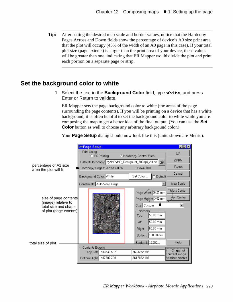
Chapter 12#Composing maps#z 1: Setting up the page
py area tal es rint
hite are
Tip: After setting the desired map scale and border values, notice that the HardcoPages Across and Down fields show the percentage of device’s A0 size printthat the plot will occupy (45% of the width of an A0 page in this case). If your toplot size (page extents) is larger than the print area of your device, these valuwill be greater than one, indicating that ER Mapper would divide the plot and peach portion on a separate page or strip.
Set the background color to white1 Select the text in the Background Color field, type white , and press
Enter or Return to validate.
ER Mapper sets the page background color to white (the areas of the page surrounding the page contents). If you will be printing on a device that has a wbackground, it is often helpful to set the background color to white while you composing the map to get a better idea of the final output. (You can use the Set Color button as well to choose any arbitrary background color.)
Your Page Setup dialog should now look like this (units shown are Metric):
total size of plot
percentage of A1 sizearea the plot will fill
size of page contents(image) relative tototal size and shapeof plot (page extents)
ER Mapper Workbook - Airphoto Mosaic Applications 223
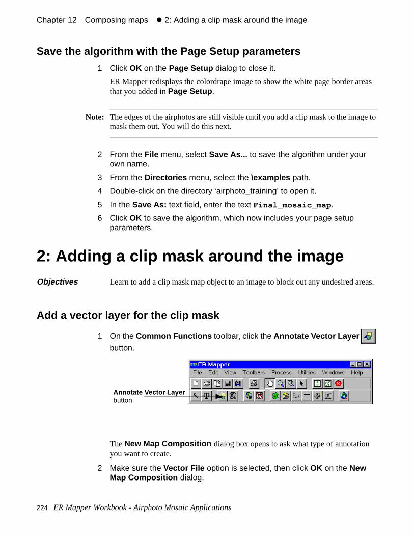
Chapter 12#Composing maps#z 2: Adding a clip mask around the image
reas
ge to
reas.
Save the algorithm with the Page Setup parameters1 Click OK on the Page Setup dialog to close it.
ER Mapper redisplays the colordrape image to show the white page border athat you added in Page Setup .
Note: The edges of the airphotos are still visible until you add a clip mask to the imamask them out. You will do this next.
2 From the File menu, select Save As... to save the algorithm under your own name.
3 From the Directories menu, select the \examples path.
4 Double-click on the directory ‘airphoto_training’ to open it.
5 In the Save As: text field, enter the text Final_mosaic_map .
6 Click OK to save the algorithm, which now includes your page setup parameters.
2: Adding a clip mask around the image
Add a vector layer for the clip mask
1 On the Common Functions toolbar, click the Annotate Vector Layer button.
The New Map Composition dialog box opens to ask what type of annotationyou want to create.
2 Make sure the Vector File option is selected, then click OK on the New Map Composition dialog.
Objectives Learn to add a clip mask map object to an image to block out any undesired a
Annotate Vector Layerbutton
224 ER Mapper Workbook - Airphoto Mosaic Applications
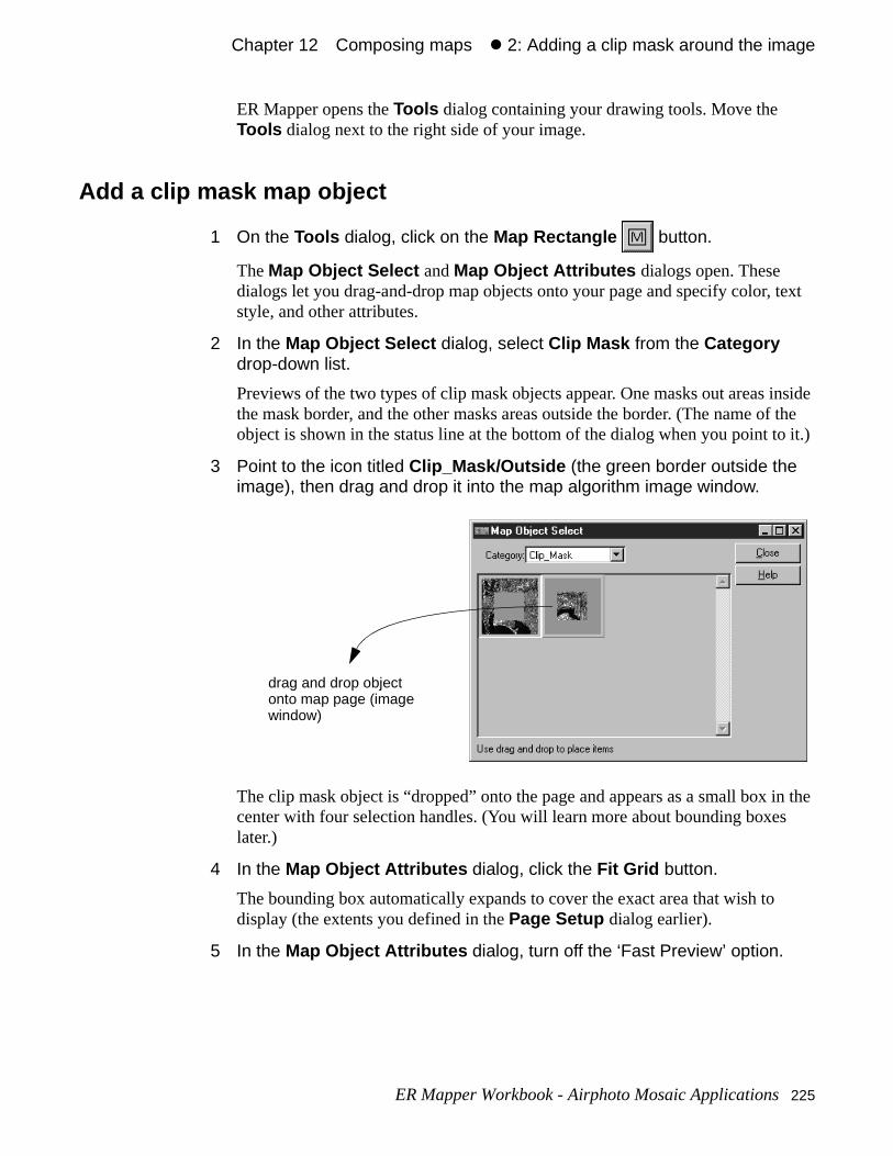
Chapter 12#Composing maps#z 2: Adding a clip mask around the image
text
inside f the it.)
in the
ER Mapper opens the Tools dialog containing your drawing tools. Move the Tools dialog next to the right side of your image.
Add a clip mask map object
1 On the Tools dialog, click on the Map Rectangle button.
The Map Object Select and Map Object Attributes dialogs open. These dialogs let you drag-and-drop map objects onto your page and specify color, style, and other attributes.
2 In the Map Object Select dialog, select Clip Mask from the Category drop-down list.
Previews of the two types of clip mask objects appear. One masks out areas the mask border, and the other masks areas outside the border. (The name oobject is shown in the status line at the bottom of the dialog when you point to
3 Point to the icon titled Clip_Mask/Outside (the green border outside the image), then drag and drop it into the map algorithm image window.
The clip mask object is “dropped” onto the page and appears as a small box center with four selection handles. (You will learn more about bounding boxeslater.)
4 In the Map Object Attributes dialog, click the Fit Grid button.
The bounding box automatically expands to cover the exact area that wish todisplay (the extents you defined in the Page Setup dialog earlier).
5 In the Map Object Attributes dialog, turn off the ‘Fast Preview’ option.
drag and drop objectonto map page (imagewindow)
ER Mapper Workbook - Airphoto Mosaic Applications 225
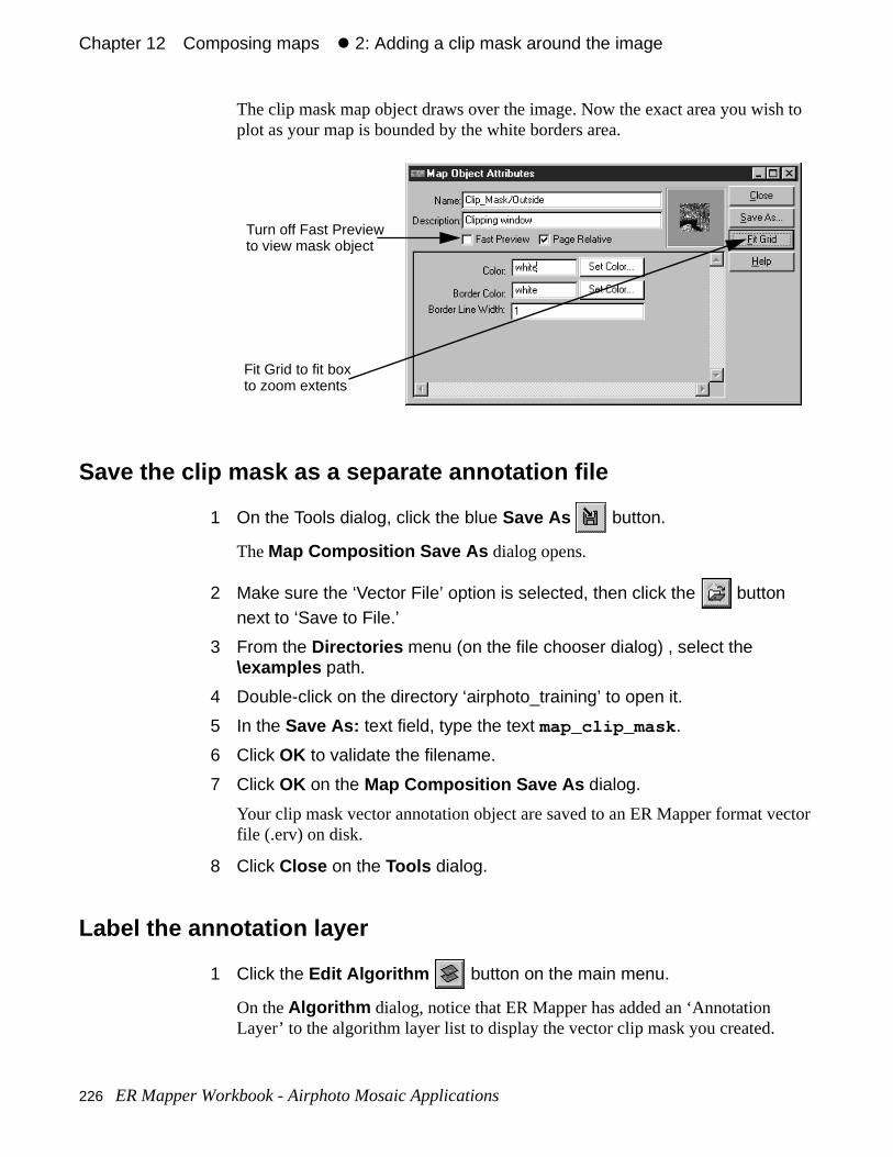
Chapter 12#Composing maps#z 2: Adding a clip mask around the image
h to
ctor
The clip mask map object draws over the image. Now the exact area you wisplot as your map is bounded by the white borders area.
Save the clip mask as a separate annotation file
1 On the Tools dialog, click the blue Save As button.
The Map Composition Save As dialog opens.
2 Make sure the ‘Vector File’ option is selected, then click the button next to ‘Save to File.’
3 From the Directories menu (on the file chooser dialog) , select the \examples path.
4 Double-click on the directory ‘airphoto_training’ to open it.
5 In the Save As: text field, type the text map_clip_mask .
6 Click OK to validate the filename.
7 Click OK on the Map Composition Save As dialog.
Your clip mask vector annotation object are saved to an ER Mapper format vefile (.erv) on disk.
8 Click Close on the Tools dialog.
Label the annotation layer
1 Click the Edit Algorithm button on the main menu.
On the Algorithm dialog, notice that ER Mapper has added an ‘Annotation Layer’ to the algorithm layer list to display the vector clip mask you created.
Fit Grid to fit boxto zoom extents
Turn off Fast Previewto view mask object
226 ER Mapper Workbook - Airphoto Mosaic Applications
Chapter 12#Composing maps#z 3: Drawing vector annotation
osaic the ter
w one.
ght.
the
2 Change the annotation layer’s label to clip mask .
3 Click Close on the Algorithm dialog to close it.
3: Drawing vector annotation
Zoom to the Page Contents and Page ExtentsCurrently the image is zoomed out to show the page extents and the relative position of the image within it.
1 Expand the image window size to make it slightly larger.
2 Right-click on the image and, from the Quick Zoom menu, select Zoom to Page Contents .
The image zooms in to the extents of the page contents (the extents of the mimage that you wish to appear in your map). Since you will draw annotation onimage, it is helpful to maximize the area on the screen used for the image. Layou will zoom to the extents again to add map objects in the border areas.
Add a second vector layer for map annotation
1 On the Common Functions toolbar, click the Annotate Vector Layer button.
The Open Map Composition dialog box opens. Since your algorithm alreadyhas one vector layer, you are prompted to reopen that dataset or create a ne
2 Click New on the Open Map Composition dialog.
The New Map Composition dialog box opens.
3 Make sure the Vector File option is selected, then click OK on the New Map Composition dialog.
ER Mapper opens the Tools dialog containing your drawing tools. Move the Tools dialog next to the right side of your image.
Draw a polyline to trace the highway in the imageThis image shows a highway running from the left center down to the lower ri
Objectives Learn to use the vector annotation tools to draw text, lines and polygons, andchange the color, style and other attributes of the objects.
ER Mapper Workbook - Airphoto Mosaic Applications 227
Chapter 12#Composing maps#z 3: Drawing vector annotation
s
s.
as
w to
lines
e.
1 On the Tools dialog, click once on the Polyline button.
2 Draw a line to trace the highway path by clicking once at each point, then double-clicking to end the line.
A line appears on your image to highlight the linear feature. Note that markerappear on the line at each node to indicate that the line is “selected.”
View and modify the attributes of the polyline
1 On the Tools dialog, double-click on the Polyline button.
The Line Style dialog box opens to let you choose attributes for your polyline
2 Click the Set Color button, choose a bright blue color, then click OK to close the Color chooser dialog.
The line color on the image changes to your selected color.
3 Click the Width drop-down list and choose 5.0 to increase the line width.
The attributes for your selected polyline change interactively.
4 On the Tools dialog, click on the Edit Object Extents button.
The Map Composition Extents dialog opens to show information about the polyline object. It shows the line length in map units, and other attributes suchthe number of vertices, geographic extents, and so on.
5 Click Close on the Map Composition Extents dialog.
6 On the Tools dialog, click the Select/Edit Points Mode button.
7 Drag any node of the selected polyline to move it.
When a polyline is selected and Select/Edit Points Mode is active, you
can reshape the line as desired by dragging the line nodes. (You will learn homove entire objects later.)
8 In the Line Style dialog, turn on the ‘Curved’ option.
ER Mapper applies a spline function to the selected line and reshapes it into smooth, rounded curves. This can be helpful to create more visually pleasingwhen tracing roads, rivers, and other curving linear features.
9 Turn off the ‘Curved’ option.
The line returns to its original appearance with straight segments at each nod
10 Click Close on the Line Style dialog.
228 ER Mapper Workbook - Airphoto Mosaic Applications
Chapter 12#Composing maps#z 3: Drawing vector annotation
to rea
ult,
Tip: To trace a long linear feature in a large image (such as this one), it is helpful draw the line along the entire extent of the feature first, then zoom into each aand adjust the exact position of the vector object by moving the line nodes.
Draw a shaded polygon around a feature
1 On the Tools dialog, click on the Polygon button.
2 Draw a polygon around any areal feature (such as a housing development) by clicking once at each point, then double-clicking to close the polygon.
The polygon object appears surrounding the area, and it is selected. By defayour polygon displays the currently selected line color, thickness, etc.
3 On the Tools dialog, double-click on the Polygon button.
The Line Style dialog box opens to let your set polygon attributes. (The samedialog is used for polylines, rectangles, and other vector objects.)
4 Click the Set Color button, choose a yellow color, then click OK to close the Color chooser dialog.
5 Under Fill Pattern , click on one of the diagonal line fill patterns.
The pattern you choose appears in the Current Fill window on the dialog. The polygon is filled with a diagonal yellow shade pattern.
6 On the Tools dialog, click on the Edit Object Extents button.
The Map Composition Extents dialog opens to show information about the polygon object, including the perimeter length and area.
7 Click Close on the Map Composition Extents dialog to close it.
Tip: To delete a node from an existing polyline or polygon, use Select/Edit Points
Mode to select it, click on the node to delete, then click the Delete Point
button. To add a node, click the Add Points Mode button, then click
on the line to add a node at that point.
Draw a shaded oval and move and resize it
1 On the Tools dialog, click the Oval button.
ER Mapper Workbook - Airphoto Mosaic Applications 229
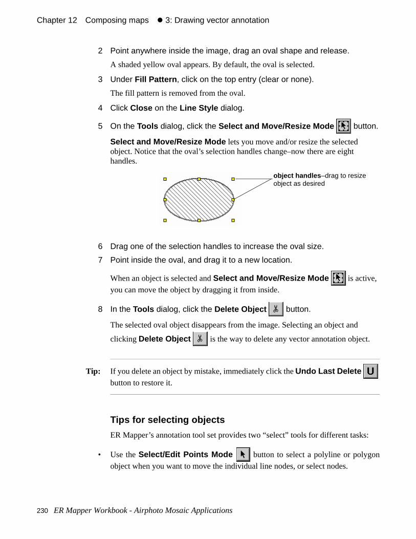
Chapter 12#Composing maps#z 3: Drawing vector annotation
:
n
2 Point anywhere inside the image, drag an oval shape and release.
A shaded yellow oval appears. By default, the oval is selected.
3 Under Fill Pattern , click on the top entry (clear or none).
The fill pattern is removed from the oval.
4 Click Close on the Line Style dialog.
5 On the Tools dialog, click the Select and Move/Resize Mode button.
Select and Move/Resize Mode lets you move and/or resize the selected object. Notice that the oval’s selection handles change–now there are eight handles.
6 Drag one of the selection handles to increase the oval size.
7 Point inside the oval, and drag it to a new location.
When an object is selected and Select and Move/Resize Mode is active,
you can move the object by dragging it from inside.
8 In the Tools dialog, click the Delete Object button.
The selected oval object disappears from the image. Selecting an object and
clicking Delete Object is the way to delete any vector annotation object.
Tip: If you delete an object by mistake, immediately click the Undo Last Delete
button to restore it.
Tips for selecting objects
ER Mapper’s annotation tool set provides two “select” tools for different tasks
• Use the Select/Edit Points Mode button to select a polyline or polygo
object when you want to move the individual line nodes, or select nodes.
object handles –drag to resizeobject as desired
230 ER Mapper Workbook - Airphoto Mosaic Applications
Chapter 12#Composing maps#z 3: Drawing vector annotation
n
e the
them
.
e
• Use the Select and Move/Resize Mode button to select any annotatio
object when you want to move the entire object (drag from the center) or resizentire object (drag one of the yellow handles).
• To select multiple objects at once, choose the Select and Move/Resize Mode
button. Then either drag a marquee box around all the objects, or select
one at a time by holding down the Shift key and clicking on them.
Tip: To duplicate an object, select it and click the Clone Object button. This can
useful, for example, for copying blocks of text or creating exact copies of polygons, ovals, and so on.
Draw and modify a text string
1 On the Tools dialog, click the Text Object button.
The Text Style dialog box opens.
2 Drag a box inside the image about one-half inch in height.
3 In the Text Style dialog, click in the Text field at the bottom to position the cursor, then type main highway .
The text appears on the image as you type.
4 In the Text Style dialog box, select the following text attributes:
Size: 72.0
Color: choose any bright color
Font Type: Postscript Stroke
Font: Helvetica-Bold
Notice that the text object automatically updates as you change the attributes
Tip: Text drawn as annotation can be set to always print at an exact point size (thFixed Text option on), or to automatically scale up or down proportionally at whatever size the image is printed (Fixed Text option off).
5 Click the Select and Move/Resize Mode button, then drag the text in the image to overlap with the blue vector you traced earlier.
6 From the Angle (deg) drop-down list, select 310.0.
ER Mapper Workbook - Airphoto Mosaic Applications 231
Chapter 12#Composing maps#z 3: Drawing vector annotation
ings
hese er
The text string rotates 310 degrees counter-clockwise, so it now points downtoward the lower right. (You can also type any arbitrary rotation value. Text strrotate around their origin in the upper-left corner.)
7 On the Tools dialog, click the Select and Move/Resize Mode button.
8 Point to the text block, and drag it to any desired position.
9 Click Close on the Text Style dialog to close it.
Place a highway number symbol on the road object
1 On the Tools dialog, click on the Map Polygon button.
The Map Object Select and Map Object Attributes dialogs open.
2 In the Map Object Select dialog, drag and drop the Road_Maps/Highway4 object onto highway line on the image.
The highway road symbol appears on the image.
3 In the Map Object Attributes dialog, set the following value (press Enter or Return afterward):
Highway: 405
Fill Color: red
The highway number and color change.
4 On the Tools dialog, click the Select and Move/Resize Mode button.
5 Resize and position the highway symbol as desired.
Tip: ER Mapper contains a wide variety of special symbols you can use in maps. Tare located on the Map Objects dialog under Map_Symbols, Symbols, and othcategories.
Save the vector objects to an annotation file
1 On the Tools dialog, click the blue Save As button.
The Map Composition Save As dialog opens.
2 Make sure the ‘Vector File’ option is selected, then click the button next to ‘Save to File.’
232 ER Mapper Workbook - Airphoto Mosaic Applications
Chapter 12#Composing maps#z 4: Defining map objects
m
rs in ple w
d
3 From the Directories menu (on the file chooser dialog) , select the \examples path.
4 Double-click on the directory ‘airphoto_training’ to open it.
5 In the Save As: text field, type the filename vector_annotation .
6 Click OK to validate the filename.
7 Click OK on the Map Composition Save As dialog.
Your vector annotation objects are saved to an ER Mapper format vector file.
8 Click Close on the Tools dialog.
Label the annotation layer
1 Click the View Algorithm for Image Window button on the main menu.
Notice that ER Mapper has added a second ‘Annotation Layer’ to the algorithlayer list to display the interpretations you create.
2 Change the annotation layer’s label to interpretations .
Note: Clip masks will cover other vector annotation if they are above the other layethe algorithm layer list. (The same priority rule that applies to overlap in multiraster layers.) It is recommended that layers for clip masks be positioned beloother vector layers unless you want to mask other vector data.
3 Click Close on the Algorithm dialog to close it.
4: Defining map objects
Zoom to the Page Extents to view the entire map page
1 On the Annotation toolbar, click the Zoom to Page Extents button.
The image zooms out to the extents of the page defined for the algorithm, anshows the white border areas where you will place map objects.
Objectives Learn to use ER Mapper’s Map Composition tools to place and modify map objects such as scale bars, coordinate grids, north arrows, and others.
ER Mapper Workbook - Airphoto Mosaic Applications 233
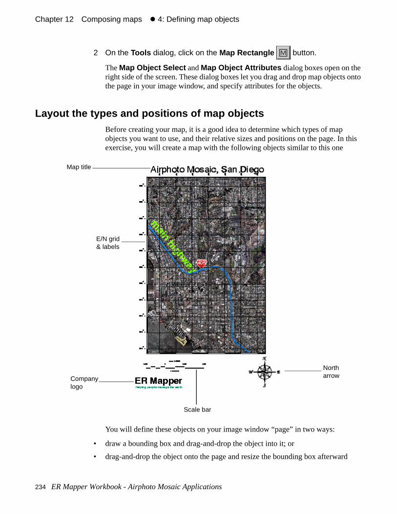
Chapter 12#Composing maps#z 4: Defining map objects
s onto
this
d
2 On the Tools dialog, click on the Map Rectangle button.
The Map Object Select and Map Object Attributes dialog boxes open on theright side of the screen. These dialog boxes let you drag and drop map objectthe page in your image window, and specify attributes for the objects.
Layout the types and positions of map objectsBefore creating your map, it is a good idea to determine which types of map objects you want to use, and their relative sizes and positions on the page. Inexercise, you will create a map with the following objects similar to this one
You will define these objects on your image window “page” in two ways:
• draw a bounding box and drag-and-drop the object into it; or
• drag-and-drop the object onto the page and resize the bounding box afterwar
Companylogo
Northarrow
E/N grid& labels
Scale bar
Map title
234 ER Mapper Workbook - Airphoto Mosaic Applications
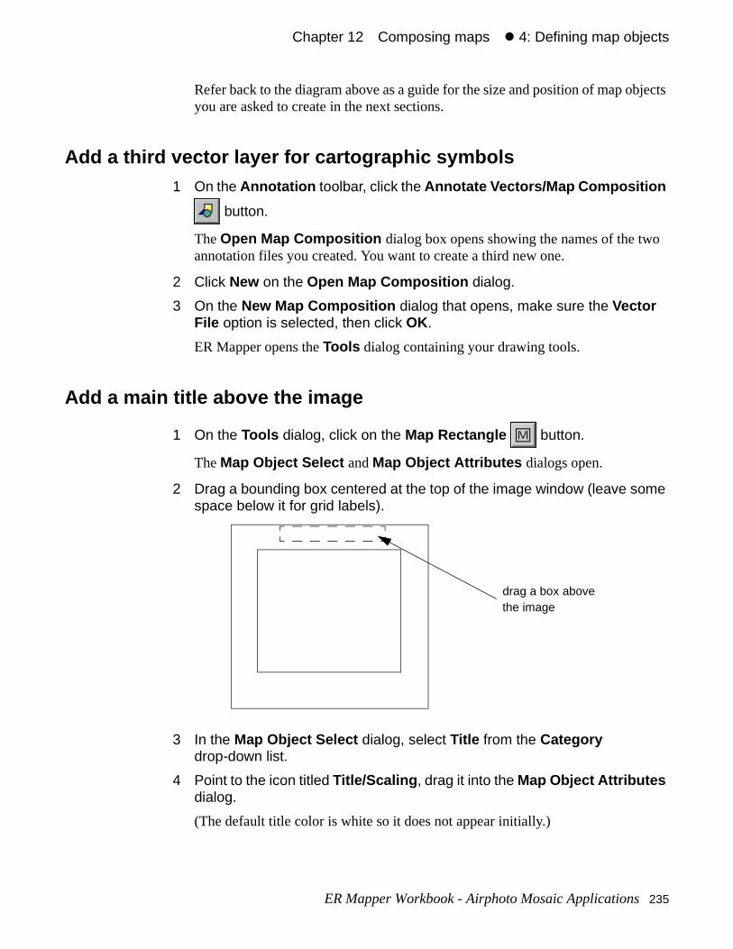
Chapter 12#Composing maps#z 4: Defining map objects
bjects
o
Refer back to the diagram above as a guide for the size and position of map oyou are asked to create in the next sections.
Add a third vector layer for cartographic symbols1 On the Annotation toolbar, click the Annotate Vectors/Map Composition
button.
The Open Map Composition dialog box opens showing the names of the twannotation files you created. You want to create a third new one.
2 Click New on the Open Map Composition dialog.
3 On the New Map Composition dialog that opens, make sure the Vector File option is selected, then click OK.
ER Mapper opens the Tools dialog containing your drawing tools.
Add a main title above the image
1 On the Tools dialog, click on the Map Rectangle button.
The Map Object Select and Map Object Attributes dialogs open.
2 Drag a bounding box centered at the top of the image window (leave some space below it for grid labels).
3 In the Map Object Select dialog, select Title from the Category drop-down list.
4 Point to the icon titled Title/Scaling , drag it into the Map Object Attributes dialog.
(The default title color is white so it does not appear initially.)
drag a box abovethe image
ER Mapper Workbook - Airphoto Mosaic Applications 235

Chapter 12#Composing maps#z 4: Defining map objects
ater.
5 On the Map Object Attributes dialog, change the following text and attributes for your title:
Title: Airphoto Mosaic, San Diego (press Enter or Return afterward)
Font Color: black (either type or use Set Color button)
The title object automatically updates as you change the attributes.
6 On the Tools dialog, click the Select and Move/Resize Mode button.
7 Resize (by dragging a handle) or reposition the title as desired.
The title text changes size automatically to fill at least one dimension of your bounding box.
Tip: If the title text is not visible, you can click on the Refresh Image button on the
Tools dialog to force ER Mapper to re-display the image.
Add a scale bar below the image1 In the Map Object Select dialog, select Scale Bar from the Category
drop-down list.
Previews of the various types of scale bar objects appear.
2 Point to the icon titled Scale_Bar/Box , then drag and drop it into a position below the image.
The scale bar object is “dropped” onto the page and it draws a few seconds lThe default attributes for the scale bar appear in the Map Object Attributes dialog box.
Zoom in on the scale bar and change the attributes
1 On the Tools dialog, click the ZoomBox Mode button.
2 Inside the image window, drag a box around the scale bar object to zoom in on it.
3 On the Map Object Attributes dialog, change the following attributes for your scale bar:
Labels Color: black
Labels Font: Helvetica-Bold (select from pop-up fonts dialog)
Units Font: Helvetica-Bold
236 ER Mapper Workbook - Airphoto Mosaic Applications
Chapter 12#Composing maps#z 4: Defining map objects
ibutes.
ally
ied
Notice that the scale bar object automatically updates as you change the attr
4 On the Annotation toolbar (on the main menu), dialog, click the Previous
Zoom button.
ER Mapper zooms out to the previous zoom level (the page extents).
5 On the Tools dialog, click the Select and Move/Resize Mode button.
6 Drag your scale bar object into the desired position, or resize it by dragging one of the selection handles.
If you resize the scale bar (make it wider or narrower), ER Mapper automaticadjusts the scale and divisions (it is a “smart” map object).
Tip: To resize or move any map object, select it first using the Select and Move/
Resize Mode button, then move or resize it as desired.
Add a north arrow on the lower-right1 In the Map Object Select dialog, select North Arrow from the Category
drop-down list.
A list of icons representing various types of north arrows appears.
2 Point to the compass north arrow (North_Arrow/Compass ), and drag it to a position in the lower-right of the page.
The north arrow object drops onto the page.
3 Click the Select and Move/Resize Mode button (on the Tools dialog), and resize and position the north arrow as desired.
Tip: ER Mapper’s north arrows are “smart” and will always point to north on a rectifimage.
Add a company logo on the lower-left1 In the Map Object Select dialog, select Logo from the Category
drop-down list.
A list of icons showing some sample company logos appears.
ER Mapper Workbook - Airphoto Mosaic Applications 237
Chapter 12#Composing maps#z 4: Defining map objects
m the
age
acing
2 Point to the ER Mapper logo icon, and drag-and-drop it onto the lower-left part of the page.
The logo object drops onto the page. Resize and position it as desired.
Tip: You can add your own company logos as Postscript files and access them frostandard Logos category used here.
Define an Eastings/Northings coordinate grid over the image1 In the Map Object Select dialog, select Grid from the Category
drop-down list.
2 Point to the Grid/EN icon, and drag it into the image window.
The grid map object draws in the lower-right part of the image.
3 On the Map Object Attributes dialog, click the Fit Grid button.
ER Mapper automatically fits the bounding box exactly to the extents of the pcontents (image) on the page.
4 On the Map Object Attributes dialog, turn on the Fast Preview option.
Fast Preview tells ER Mapper not to update the object interactively as you change the attributes.
5 On the Map Object Attributes dialog, change the following attributes for your grid (use defaults for all others):
Grid Style: Full Grid
Border Type: Checks
Grid Spacing X: 500 meters
Grid Spacing Y: 500 meters
Top labels orientation: Horizontal Right
Tip: You could have used the grid to clip the image without having a separate clipmask. To do this you would select the Clip option.
6 On the Map Object Attributes dialog, turn off the Fast Preview option.
The grid map object is rendered using the attributes you defined. The grid spis 500 meters, and the “checks” option puts a map collar around the image.
238 ER Mapper Workbook - Airphoto Mosaic Applications
Chapter 12#Composing maps#z 4: Defining map objects
nge
er
zing
.
Tip: The Fast Preview option is very useful for working with complex map objectsthat take time to redraw (such as a grid or algorithm image). This lets you chaall the attributes you desire or fine tune object size/position without ER Mapptrying to update the object on the screen each time.
Adjust the size or position of any objectIf desired, you can easily resize or position any map object by moving or resithe bounding box that contains it.
1 In the Tools palette dialog, click the Select and Move/Resize Mode button.
2 Click on any map object to select it (the handles will appear), and drag the bounding box to reposition it or change the size by dragging a handle.
Save the map composition file to disk
1 On the Tools dialog, click the blue Save As button.
The Map Composition Save As dialog opens.
2 Make sure the ‘Vector File’ option is selected, then click the button next to ‘Save to File.’
3 From the Directories menu (on the file chooser dialog) , select the \examples path.
4 Double-click on the directory ‘airphoto_training’ to open it.
5 In the Save As: text field, type the text map_composition .
6 Click OK to validate the filename.
7 Click OK on the Map Composition Save As dialog.
Your map objects are saved to an ER Mapper format vector file (.erv) on disk
8 Click Close on the Tools dialog.
Note: When you close the Tools dialog (exit edit mode), ER Mapper redisplays the image exactly as it will look when printed. (During edit mode, line thickness isslightly exaggerated to help editing and modifications.)
ER Mapper Workbook - Airphoto Mosaic Applications 239
Chapter 12#Composing maps#z 4: Defining map objects
p
s you jects. d
file.)
. n
s
Label the map composition layer
1 Click the View Algorithm for Image Window button on the main menu.
On the Algorithm dialog, you now have three annotation layers–your new maobjects layer, your ‘vector annotation’ layer, and your ‘clip mask’ layer.
2 Change the ‘Annotation Layer’ label to map composition .
3 Click Close on the Algorithm dialog to close it.
Tip: It is often helpful to separate different types of annotation into separate files adid here–one for a clip mask, one for vector drawing, and another for map obThis makes it easier to work with the data, and you can simply turn the desirevector layers on/off to display/not display those items in your algorithm. (You could have saved all your vector interpretations and map objects in the same
Save the algorithm to update the changes
1 On the main menu, click the Save toolbar button.
2 When asked to confirm the overwrite, click OK.
Your algorithm can now be printed using the Print toolbar button or by
selecting Print from the File menu.
Note: It is important to remember to save your algorithm after defining map objectsOtherwise the annotation layers and files will not be part of the algorithm wheyou go to print it later.
Close all image windows and dialog boxes1 Close the image window using the window system controls or by selecting
Close from the File menu.
Only the ER Mapper main menu should be open on the screen.
• Define Page Setup parameters for an algorithm
What you learned...
After completing these exercises, you know how to perform the following taskin ER Mapper:
240 ER Mapper Workbook - Airphoto Mosaic Applications
Chapter 12#Composing maps#z 4: Defining map objects
Map r on
e oldrrows,
ticallyve ale bar
te in
r own
cts on
e, or
the
ge
ize
main or the
its.
• Add an Annotation/Map Composition layer to an algorithm
• Add a clip mask around the image
• Draw annotation objects (lines, text, polygons, etc.) on your map
• Place map objects (grids, scale bars, etc.) on your map
• Specify color and other attributes for annotation and map objects
Additional features of Map CompositionThe preceding simple example covered only the basics of using ER Mapper’sComposition, and following are some additional features. Refer to the chaptecreating maps in the ER Mapper User Guide for complete information.
• If you drag an object into a bounding box that already contains an object, thobject is replaced by the new one. This is an easy way to try several north afor example.
• Objects that are dragged and dropped to replace a current object automainherit any common attributes from the previous object. For example, if you hared north arrow in a bounding box and then drag in a scale bar object, the scaautomatically inherits the red color (since both objects have the “Color” attribucommon).
• You can modify the default attributes of map objects and save them under younames (using Save As on the Map Object Attributes dialog).
• You can draw other image processing algorithms you’ve created as map objethe page (using the Category: Algorithm on the Map Object Select dialog).This is useful for drawing inset images that show an overview map, inset imagother types of processing techniques or data of the same area.
• You can plot objects from external files like TIFF, EPS, or Targa (usingCategory: Image on the Map Object Select dialog)
• You can import text directly from ASCII text files and plot it on your map pa(using the Category: Text on the Map Object Select dialog)
Page Relative and Map Unit Relative map objectsThe vector map objects you defined in this exercise have their position and sspecified relative to the page, rather than to map units (such as Latitude Longitude). This allows you to create standard map sheets with objects that rein a fixed size and position on the page, regardless of how the page is scaledextents of the datasets used in the page contents are changed.
You can also specify the position of map objects in geographic coordinate unThe position of each object is tied to a particular geographic location and mapsheet size.
ER Mapper Workbook - Airphoto Mosaic Applications 241
Chapter 12#Composing maps#z 4: Defining map objects
ge.
ugh re
s,s of thended
sizeode is
raining(pagehis is ag the
ges mode
apis mode scale
ll the
To specify a map object as map unit relative, turn off the Page Relative option on the Map Object Attribute dialog box. The page relative attribute can be assigned either before or after the object is dragged-and-dropped onto the paSee the ER Mapper User Guide for more information.
Page Setup Constraints optionsIn the previous simple example, you chose the ‘Auto Vary:Page’ option, althoyou could have chosen others as well. The Constraints options you can use asummarized briefly below:
• Fixed Page:Extents from Zoom–This is the default setting for all new algorithmwhere the contents scale and borders are taken from the current zoom extentalgorithm. For map making purposes, Extents from Zoom is not recommebecause it can effect line thickness and text sizing.
• Auto Vary:Page–This mode allows ER Mapper to automatically vary the page to account for any changes made to the map scale or page borders. This measiest, for example, to print a map at an exact scale without regards to constit to a specific page size. If you want to place map objects outside the image contents) area, enter the desired border sizes to create space for them. (Tgood initial choice when you are prompted to change the mode when usinannotation tools.)
• Auto Vary:Borders–This mode allows ER Mapper to automatically vary the paborders to account for any changes made to the map scale or page size. Thiis most useful for printing at both an exact map scale and exact plot size.
• Auto Vary:Scale–This mode allows ER Mapper to automatically vary the mscale to account for any changes made to the page size or page borders. This useful, for example, for printing an image at various sizes when exact mapis not important.
Printing your mapWhen you want to print your final map algorithm (using File/Print or the Print
button), ER Mapper asks for the name of the algorithm. When the print
operation begins, ER Mapper automatically locates, processes and renders a
242 ER Mapper Workbook - Airphoto Mosaic Applications
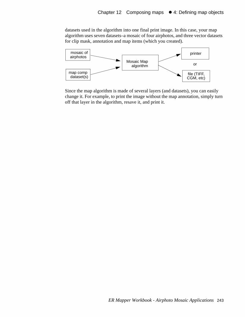
Chapter 12#Composing maps#z 4: Defining map objects
p atasets
sily turn
datasets used in the algorithm into one final print image. In this case, your maalgorithm uses seven datasets–a mosaic of four airphotos, and three vector dfor clip mask, annotation and map items (which you created).
Since the map algorithm is made of several layers (and datasets), you can eachange it. For example, to print the image without the map annotation, simplyoff that layer in the algorithm, resave it, and print it.
mosaic ofairphotos
map compdataset(s)
Mosaic Mapalgorithm
printer
file (TIFF,CGM, etc)
or
ER Mapper Workbook - Airphoto Mosaic Applications 243

Chapter 12#Composing maps#z 4: Defining map objects
244 ER Mapper Workbook - Airphoto Mosaic Applications
ge.
h
1 of its
own lly ell
ry wide ,
13
Compressingimages
This chapter shows you how to save your large mosaic as a compressed ima
About ECW compressionER Mapper compresses images using wavelet compression technology whicoffers very high quality results at high compression rates. You can typically compress a color image to less than 2% to 5% of its original size (50:1 to 20:compression ratio) and compress a grayscale image to less than 5% to 10% original size (20:1 to 10:1 compression ratio).
This means that, at 20:1 compression, 10GB of color imagery will compress dto 500MB, which is small enough to fit on to a single CD-ROM. You may actuaachieve higher compression rates where your source image has a structure wsuited to compression.
In addition to reducing storage requirements, you can also use the free imageplug-ins for GIS and office applications to read the compressed imagery in a range of software applications such as ArcView®, AutoCAD MAP®, MapInfo®ER Viewer, Photoshop™, Microsoft Office® and Excel®, and other software applications.
ER Mapper Workbook - Airphoto Mosaic Applications 245
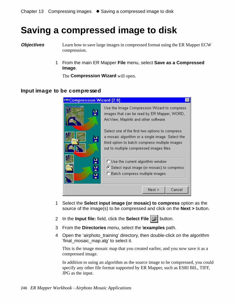
Chapter 13#Compressing images#z Saving a compressed image to disk
s a
could F,
CW
Saving a compressed image to disk
1 From the main ER Mapper File menu, select Save as a Compressed Image .
The Compression Wizard will open.
Input image to be compressed
1 Select the Select input image (or mosaic) to compress option as the source of the image(s) to be compressed and click on the Next > button.
2 In the Input file: field, click the Select File button.
3 From the Directories menu, select the \examples path.
4 Open the ‘airphoto_training’ directory, then double-click on the algorithm ‘final_mosaic_map.alg’ to select it.
This is the image mosaic map that you created earlier, and you now save it acompressed image.
In addition to using an algorithm as the source image to be compressed, you specify any other file format supported by ER Mapper, such as ESRI BIL, TIFJPG as the input.
Objectives Learn how to save large images in compressed format using the ER Mapper Ecompression.
246 ER Mapper Workbook - Airphoto Mosaic Applications
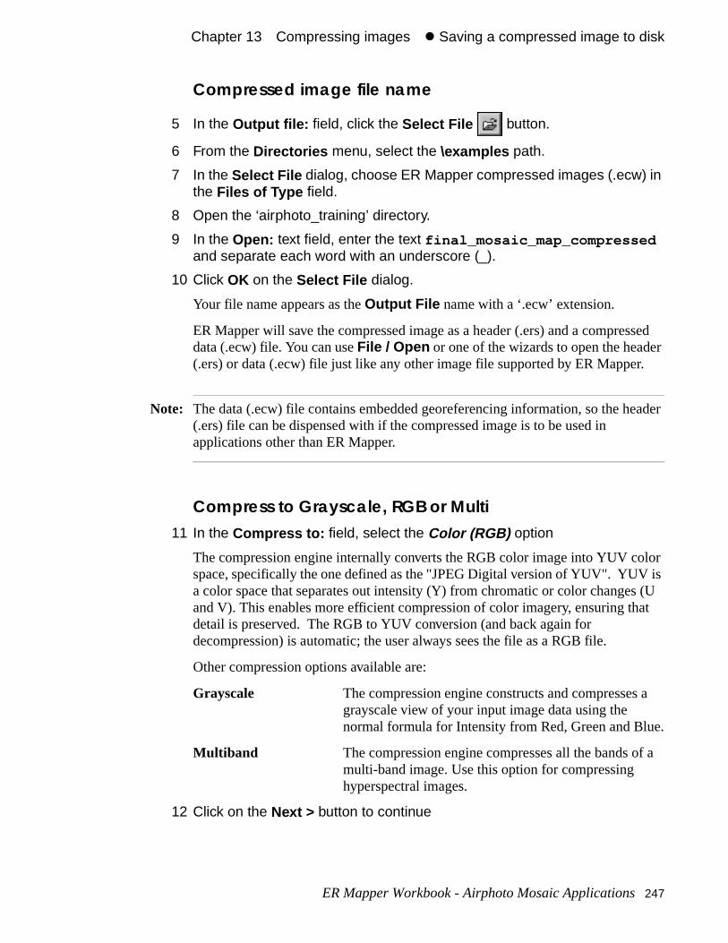
Chapter 13#Compressing images#z Saving a compressed image to disk
ssed er r.
eader
olor is
s (U at
a
e.
f a
Compressed image file name
5 In the Output file: field, click the Select File button.
6 From the Directories menu, select the \examples path.
7 In the Select File dialog, choose ER Mapper compressed images (.ecw) in the Files of Type field.
8 Open the ‘airphoto_training’ directory.
9 In the Open: text field, enter the text final_mosaic_map_compressed and separate each word with an underscore (_).
10 Click OK on the Select File dialog.
Your file name appears as the Output File name with a ‘.ecw’ extension.
ER Mapper will save the compressed image as a header (.ers) and a compredata (.ecw) file. You can use File / Open or one of the wizards to open the head(.ers) or data (.ecw) file just like any other image file supported by ER Mappe
Note: The data (.ecw) file contains embedded georeferencing information, so the h(.ers) file can be dispensed with if the compressed image is to be used in applications other than ER Mapper.
Compress to Grayscale, RGB or Multi11 In the Compress to: field, select the Color (RGB) option
The compression engine internally converts the RGB color image into YUV cspace, specifically the one defined as the "JPEG Digital version of YUV". YUVa color space that separates out intensity (Y) from chromatic or color changeand V). This enables more efficient compression of color imagery, ensuring thdetail is preserved. The RGB to YUV conversion (and back again for decompression) is automatic; the user always sees the file as a RGB file.
Other compression options available are:
Grayscale The compression engine constructs and compressesgrayscale view of your input image data using the normal formula for Intensity from Red, Green and Blu
Multiband The compression engine compresses all the bands omulti-band image. Use this option for compressing hyperspectral images.
12 Click on the Next > button to continue
ER Mapper Workbook - Airphoto Mosaic Applications 247
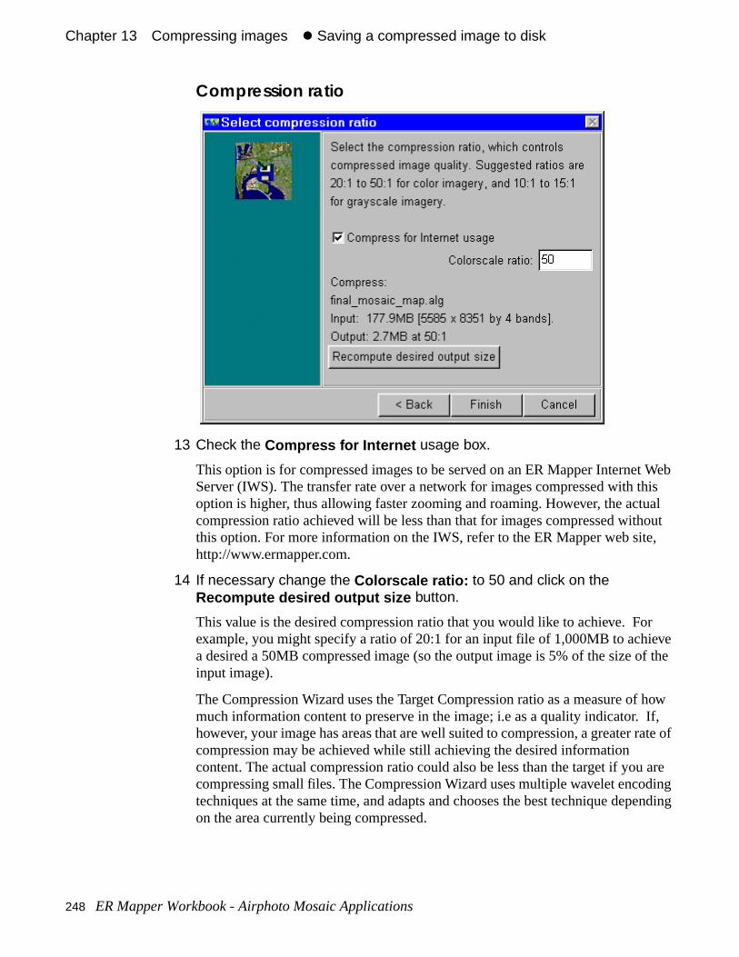
Chapter 13#Compressing images#z Saving a compressed image to disk
t Web his al out ,
r ve
of the
f how If, rate of
are ding
pending
Compression ratio
13 Check the Compress for Internet usage box.
This option is for compressed images to be served on an ER Mapper InterneServer (IWS). The transfer rate over a network for images compressed with toption is higher, thus allowing faster zooming and roaming. However, the actucompression ratio achieved will be less than that for images compressed withthis option. For more information on the IWS, refer to the ER Mapper web sitehttp://www.ermapper.com.
14 If necessary change the Colorscale ratio: to 50 and click on the Recompute desired output size button.
This value is the desired compression ratio that you would like to achieve. Foexample, you might specify a ratio of 20:1 for an input file of 1,000MB to achiea desired a 50MB compressed image (so the output image is 5% of the size input image).
The Compression Wizard uses the Target Compression ratio as a measure omuch information content to preserve in the image; i.e as a quality indicator. however, your image has areas that are well suited to compression, a greater compression may be achieved while still achieving the desired information content. The actual compression ratio could also be less than the target if youcompressing small files. The Compression Wizard uses multiple wavelet encotechniques at the same time, and adapts and chooses the best technique deon the area currently being compressed.
248 ER Mapper Workbook - Airphoto Mosaic Applications
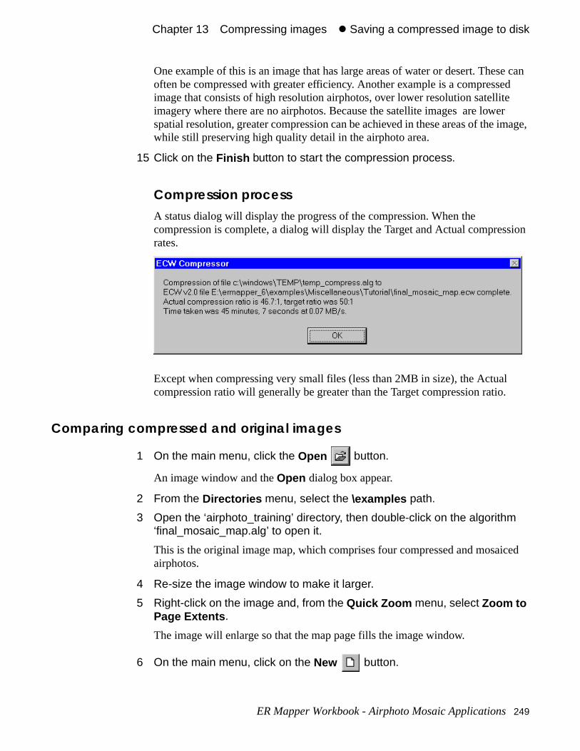
Chapter 13#Compressing images#z Saving a compressed image to disk
e can d r image,
sion
.
ced
One example of this is an image that has large areas of water or desert. Thesoften be compressed with greater efficiency. Another example is a compresseimage that consists of high resolution airphotos, over lower resolution satelliteimagery where there are no airphotos. Because the satellite images are lowespatial resolution, greater compression can be achieved in these areas of the while still preserving high quality detail in the airphoto area.
15 Click on the Finish button to start the compression process.
Compression processA status dialog will display the progress of the compression. When the compression is complete, a dialog will display the Target and Actual compresrates.
Except when compressing very small files (less than 2MB in size), the Actualcompression ratio will generally be greater than the Target compression ratio
Comparing compressed and original images
1 On the main menu, click the Open button.
An image window and the Open dialog box appear.
2 From the Directories menu, select the \examples path.
3 Open the ‘airphoto_training’ directory, then double-click on the algorithm ‘final_mosaic_map.alg’ to open it.
This is the original image map, which comprises four compressed and mosaiairphotos.
4 Re-size the image window to make it larger.
5 Right-click on the image and, from the Quick Zoom menu, select Zoom to Page Extents .
The image will enlarge so that the map page fills the image window.
6 On the main menu, click on the New button.
ER Mapper Workbook - Airphoto Mosaic Applications 249
Chapter 13#Compressing images#z Saving a compressed image to disk
e up te ps to
es.
.
This will open a second image window.
7 On the main menu, click the Open button.
An image window and the Open dialog box appear.
8 In the Files of Type: field, select ‘ER Mapper compressed images (.ecw)’.
9 From the Directories menu, select the \examples path.
10 Open the ‘airphoto_training’ directory, then double-click on the file ‘final_mosaic_map_compressed.ecw’ to open it.
This is the compressed image file that you have just created.
11 Re-size this new image window to make it the same size as the other.
12 Right-click on the image and, from the Quick Zoom menu, select Zoom to All Datasets .
The image will enlarge to fill the image window.
13 Move the image windows so that they are next to one another.
14 Compare the quality of the two images.
The quality should be virtually identical because the original mosaic was madof individually compressed images. This is an example of how you could creamosaics with thousands of large images while conserving disk space. The stefollow are:
1. After geocoding the images, compress them and store them on disk.
2. Use the Image Display and Mosaic Wizard to mosaic the compressed imag
3. Use the Balancing Wizard to balance and color match the mosaiced image
4. Use the Compression Wizard to compress the final image.
250 ER Mapper Workbook - Airphoto Mosaic Applications
Chapter 13#Compressing images#z Saving a compressed image to disk
in
Close both image windows and dialog boxes1 Close the image window using the window system controls:
• For Windows, click the Close button in the upper-right window corner.
2 Click Close on the Algorithm dialog.
Only the ER Mapper main menu should be open on the screen
• Save the image in compressed format using the ECW compressor.
What you learned
After completing these exercises, you know how to perform the following tasksER Mapper:
ER Mapper Workbook - Airphoto Mosaic Applications 251

Chapter 13#Compressing images#z Saving a compressed image to disk
252 ER Mapper Workbook - Airphoto Mosaic Applications

or use
to
the ge
ts, sed to
tor ata.
14
Exporting to GISsystems
This chapter shows you how to save all or part of a processed mosaic image fin a GIS or desktop mapping software product.
About use in GIS systemsOnce you have created your mosaic of images in ER Mapper, you may want save all or part of the mosaic image in a format suitable for use in a GIS or Desktop Mapping System (DMS). The procedure you will use depends upon raster formats your GIS can accept, and its capabilities for handling large imadatasets.
Note: ER Mapper provides free plug-ins to most GIS or Desktop Mapping System applications, which allow you to open ER Mapper images directly in those applications. Formats supported include ER Mapper algorithms, raster datasevirtual datasets and ECW compressed images. Where possible, you are adviuse these plug-ins which are available for download at www.ermapper.com .
Since GIS and desktop mapping systems are usually designed to handle vec(line/polygon) data, they have limited capabilities for handling raster (image) dFor example, ER Mapper has no problem handling a 20,000 by 20,000 pixel
ER Mapper Workbook - Airphoto Mosaic Applications 253
Chapter 14#Exporting to GIS systems#z About use in GIS systems
an ssible
hieved useion.
muchake
ring a and
stillution
t an asic
with
UDFr to a
one
geolutionduct.
otneral-meter
ed forn.
image, but few GIS or DMS applications can do this. When preparing to saveenhanced image from ER Mapper for use in a GIS or DMS, there are three posolutions to this problem:
• Save the image in ECW compressed format. The high compression rates acby using this format make the image files significantly smaller. You can thenthe applicable free plug-in to open the compressed image in the GIS applicat
• Resample the image to a lower spatial resolution (cell size). This creates smaller files, but you lose detail in the image. This may be best if you want to ma single image file that covers a large geographic area.
• Subset the airphoto (or mosaic) image into a set of smaller files, each covesmaller geographic area. This maintains the original detail in the airphotoscreates individual files small enough for your GIS or DMS to handle. (It requires a large amount of disk space to store all the individual high resolfiles.)
Cropping or subsetting images
Often you will want to crop or subset part of the entire mosaic that covers jusarea of interest, or subset a large mosaic into smaller pieces. There are two bsteps:
• Zoom into the desired area. You can do this visually by dragging a zoom boxthe the mouse, or by entering exact coordinates in the Algorithm GeopositionExtents dialog.
• Save the area of interest to an external file. You can save to an ER Mapper(Universal Data Format) dataset (which can be read by many systems), ographics file such as TIFF.
Spatial resolution (cell size)
Digitized aerial photos are often created at very high resolution; for example meter pixel size or even less. This creates very large image files that can be hundreds of megabytes in size. There are two reasons why you may want to consider reducing the spatial resolution (cell size) of the exported image:
• GIS/DMS file size limitations–If you want to use an image covering a largeographic area, you may need to resample the image to a lower spatial res(larger cell size), thus creating a smaller file that can be handled by the GIS pro
• Detail required for the project–The amount of detail in airphotos is often nneeded for a particular application or project. For example, for updating a geland use database, it may not be necessary to use imagery with less than 1resolution. If desired, you can resample the image to the level of detail needthe project to create files that are only as large as necessary for the applicatio
254 ER Mapper Workbook - Airphoto Mosaic Applications
Chapter 14#Exporting to GIS systems#z Using compressed images in GIS systems
cts ou
taile,e
ely,fo toally
grate
or
to y.
r use ou en g
rk
ge,
Raster formats for GIS and DMS products
The two most common formats accepted by GIS and DMS products are TIFF(Tagged Image File Format) and BIL (band interleaved by line) format. ER Mapper’s native format is binary BIL, so that is the best solution for produthat can read BIL format. Use the following guide to determine which format yneed to use:
• ArcView® OR ARC/INFO® –Create an ER Mapper UDF (Universal DaFormat) dataset (in BIL format), which, in addition to the “.ers” header fincludes a “.hdr” file that allows ArcView® or ARC/INFO® to read the BIL fildirectly.
• Autodesk World™, AutoCAD MAP® or AutoCAD® –Use ER Mapper to savethe image to a TIFF format file.
• MapInfo –Use ER Mapper to save the image to a TIFF format file. AlternativER Mapper also provides a free upgrade to MapInfo users that allows MapIndirectly read ER Mapper format image files and algorithms. The link automaticpasses the map projection information to MapInfo. This allows users to intevery large mosaics of imagery as backdrops into MapInfo quickly and easily.
• Other GIS and DMS products–Use ER Mapper to save the image to a TIFFother compatible graphics format file.
Using compressed images in GIS systemsThe ECW Compression Wizard, which is included in ER Mapper, enables yousave large images in the ECW compressed format with minimal loss in qualitCompression rates can typically be in the order of 50:1.
The relatively small file sizes of ECW compressed images make them ideal foin GIS applications. The free plug-ins available for many GIS products allow yto open ECW compressed images directly in those products. You can also opECW compressed images served over a network (e.g. the Internet) by enterintheir URLs. You can then roam over and zoom into the image over the netwofrom within the application.
Hands-on exercisesThese exercises show you how to crop an area of interest from a mosaic imasave the area as an ER Mapper UDF dataset and a TIFF file.
What you will learn...
After completing these exercises, you will know how to perform the following tasks in ER Mapper:
ER Mapper Workbook - Airphoto Mosaic Applications 255
Chapter 14#Exporting to GIS systems#z 1: Defining an area of interest
terest
pacts ls for eters)
are
• Define an exact area of interest using geographic coordinates
• Save the image as a new UDF dataset
• Resample the resolution (cell size) of a dataset
• Save an image as a TIFF format graphics file
1: Defining an area of interest
Open the final mosaic algorithm1 On the main menu, select Open from the File menu.
An image window and the Open dialog appear.
2 From the Directories menu (on the Open dialog), select the path ending with \examples .
3 Double-click to open the directory named ‘airphoto_training.’
4 Double-click on your ‘airphoto_mosaic.balanced.alg’ algorithm to open it.
The balanced RGB mosaic image displays. Next you define a small area of infor your project.
Zoom into the project areaAssume that you have a project to assess the progress and environmental imof the highway interchange in the centre of the mosaic image. The project calan image showing an exact area defined by Easting and Northings values (min the UTM projection being used.
1 From the View menu, select Geoposition .
The Algorithm Geoposition Extents dialog opens.
2 Click the Extents tab to display the current mosaic extents.
3 Enter the following values in the Eastings and Northings Top Left and Bottom Right fields:
Top Left - Easting: 484979
Before you begin...
Before beginning these exercises, make sure all ER Mapper image windows closed. Only the ER Mapper main menu should be open on the screen.
Objectives Learn to define exact areas of interest in an image, and how to subsection animage into smaller files.
256 ER Mapper Workbook - Airphoto Mosaic Applications
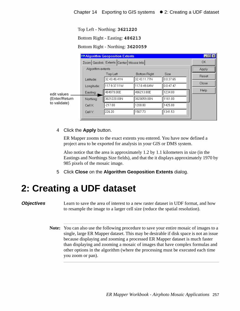
Chapter 14#Exporting to GIS systems#z 2: Creating a UDF dataset
0 by
s to a issue ster and time
how
Top Left - Northing: 3621220
Bottom Right - Easting: 486213
Bottom Right - Northing: 3620059
4 Click the Apply button.
ER Mapper zooms to the exact extents you entered. You have now defined aproject area to be exported for analysis in your GIS or DMS system.
Also notice that the area is approximately 1.2 by 1.1 kilometers in size (in theEastings and Northings Size fields), and that the it displays approximately 197985 pixels of the mosaic image.
5 Click Close on the Algorithm Geoposition Extents dialog.
2: Creating a UDF dataset
Note: You can also use the following procedure to save your entire mosaic of imagesingle, large ER Mapper dataset. This may be desirable if disk space is not anbecause displaying and zooming a processed ER Mapper dataset is much fathan displaying and zooming a mosaic of images that have complex formulasother options in the algorithm (where the processing must be executed each you zoom or pan).
Objectives Learn to save the area of interest to a new raster dataset in UDF format, andto resample the image to a larger cell size (reduce the spatial resolution).
edit values(Enter/Returnto validate)
ER Mapper Workbook - Airphoto Mosaic Applications 257
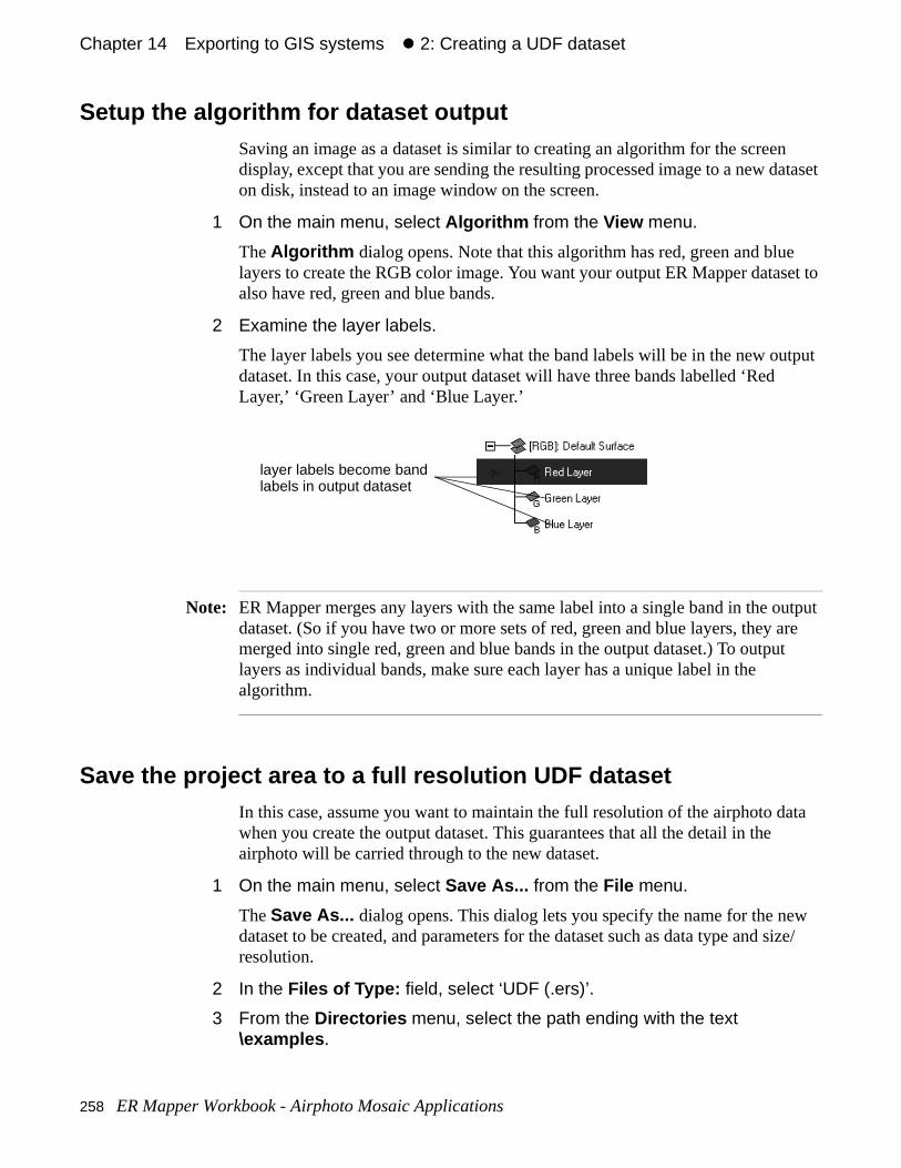
Chapter 14#Exporting to GIS systems#z 2: Creating a UDF dataset
n ataset
et to
tput
utput are t
ata
w size/
Setup the algorithm for dataset outputSaving an image as a dataset is similar to creating an algorithm for the screedisplay, except that you are sending the resulting processed image to a new don disk, instead to an image window on the screen.
1 On the main menu, select Algorithm from the View menu.
The Algorithm dialog opens. Note that this algorithm has red, green and bluelayers to create the RGB color image. You want your output ER Mapper datasalso have red, green and blue bands.
2 Examine the layer labels.
The layer labels you see determine what the band labels will be in the new oudataset. In this case, your output dataset will have three bands labelled ‘Red Layer,’ ‘Green Layer’ and ‘Blue Layer.’
Note: ER Mapper merges any layers with the same label into a single band in the odataset. (So if you have two or more sets of red, green and blue layers, they merged into single red, green and blue bands in the output dataset.) To outpulayers as individual bands, make sure each layer has a unique label in the algorithm.
Save the project area to a full resolution UDF datasetIn this case, assume you want to maintain the full resolution of the airphoto dwhen you create the output dataset. This guarantees that all the detail in the airphoto will be carried through to the new dataset.
1 On the main menu, select Save As... from the File menu.
The Save As... dialog opens. This dialog lets you specify the name for the nedataset to be created, and parameters for the dataset such as data type and resolution.
2 In the Files of Type: field, select ‘UDF (.ers)’.
3 From the Directories menu, select the path ending with the text \examples .
layer labels become bandlabels in output dataset
258 ER Mapper Workbook - Airphoto Mosaic Applications
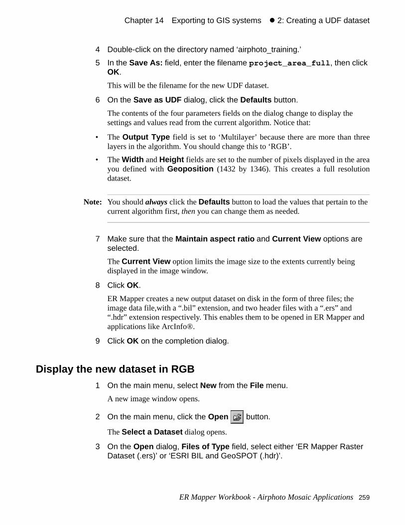
Chapter 14#Exporting to GIS systems#z 2: Creating a UDF dataset
ree
rean
e
and
4 Double-click on the directory named ‘airphoto_training.’
5 In the Save As: field, enter the filename project_area_full , then click OK.
This will be the filename for the new UDF dataset.
6 On the Save as UDF dialog, click the Defaults button.
The contents of the four parameters fields on the dialog change to display thesettings and values read from the current algorithm. Notice that:
• The Output Type field is set to ‘Multilayer’ because there are more than thlayers in the algorithm. You should change this to ‘RGB’.
• The Width and Height fields are set to the number of pixels displayed in the ayou defined with Geoposition (1432 by 1346). This creates a full resolutiodataset.
Note: You should always click the Defaults button to load the values that pertain to thcurrent algorithm first, then you can change them as needed.
7 Make sure that the Maintain aspect ratio and Current View options are selected.
The Current View option limits the image size to the extents currently being displayed in the image window.
8 Click OK.
ER Mapper creates a new output dataset on disk in the form of three files; theimage data file,with a “.bil” extension, and two header files with a “.ers” and “.hdr” extension respectively. This enables them to be opened in ER Mapper applications like ArcInfo®.
9 Click OK on the completion dialog.
Display the new dataset in RGB1 On the main menu, select New from the File menu.
A new image window opens.
2 On the main menu, click the Open button.
The Select a Dataset dialog opens.
3 On the Open dialog, Files of Type field, select either ‘ER Mapper Raster Dataset (.ers)’ or ‘ESRI BIL and GeoSPOT (.hdr)’.
ER Mapper Workbook - Airphoto Mosaic Applications 259
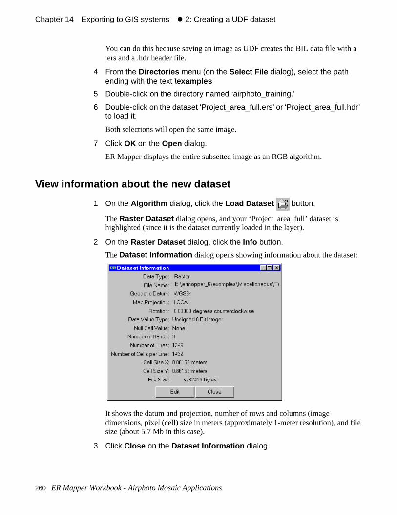
Chapter 14#Exporting to GIS systems#z 2: Creating a UDF dataset
ith a
t:
file
You can do this because saving an image as UDF creates the BIL data file w.ers and a .hdr header file.
4 From the Directories menu (on the Select File dialog), select the path ending with the text \examples
5 Double-click on the directory named ‘airphoto_training.’
6 Double-click on the dataset ‘Project_area_full.ers’ or ‘Project_area_full.hdr’ to load it.
Both selections will open the same image.
7 Click OK on the Open dialog.
ER Mapper displays the entire subsetted image as an RGB algorithm.
View information about the new dataset
1 On the Algorithm dialog, click the Load Dataset button.
The Raster Dataset dialog opens, and your ‘Project_area_full’ dataset is highlighted (since it is the dataset currently loaded in the layer).
2 On the Raster Dataset dialog, click the Info button.
The Dataset Information dialog opens showing information about the datase
It shows the datum and projection, number of rows and columns (image dimensions, pixel (cell) size in meters (approximately 1-meter resolution), andsize (about 5.7 Mb in this case).
3 Click Close on the Dataset Information dialog.
260 ER Mapper Workbook - Airphoto Mosaic Applications
Chapter 14#Exporting to GIS systems#z 2: Creating a UDF dataset
like ller t t half size ges.)
w size/
teger
Save the project area to a half resolution UDF datasetLet us assume that the full detail in the airphoto is not needed, and you wouldto resample the image to approximately two-meter resolution to create a smafile for your GIS. One way to do this is to follow the same steps as before, budivide the default image width and height values by two to create a dataset athe original resolution. (You may also want to do this simply to reduce the file when covering a large area if your GIS or DMS cannot handle very large ima
1 Activate the image window containing the original mosaic image (named ‘Final_RGB_mosaic’).
The contents of the Algorithm dialog change to show the mosaic algorithm.
2 On the main menu, select Save As... from the File menu.
The Save As... dialog opens. This dialog lets you specify the name for the nedataset to be created, and parameters for the dataset such as data type and resolution.
3 In the Files of Type: field, select ‘UDF (.ers)’.
4 From the Directories menu, select the path ending with the text \examples .
5 Double-click on the directory named ‘airphoto_training.’
6 In the Save As: field, enter the filename project_area_half , then click OK.
This will be the filename for the new UDF dataset.
7 On the Save as UDF dialog, click the Defaults button.
The contents of the four parameters fields on the dialog change to display thesettings and values read from the current algorithm.
8 Open the Output Type field, select ‘RGB’.
As before, this tells ER Mapper to rescale the real data values into an 8-bit in(0-255) data range in the output dataset.
9 Change the values in the Width and Height fields as follows (the original values divided by 2 and rounded up):
Cells Across (width) = 716
Cells Down (height) = 673
10 Click OK, then click Yes when asked to confirm the dataset creation.
ER Mapper creates a new half-resolution output dataset on disk.
11 Click OK on the completion dialog.
ER Mapper Workbook - Airphoto Mosaic Applications 261
Chapter 14#Exporting to GIS systems#z 2: Creating a UDF dataset
your new ses age,
ting does
ith a
m.
Note: When creating a new dataset with different cell sizes to the original data, ER Mapper resamples the original data to the new output cell size during theprocess of creating the new dataset. If the ‘Smoothing’ button is turned on in algorithm (as in this case), ER Mapper uses bilinear interpolation to create theoutput dataset cell values. If the ‘Smoothing’ button is turned off, ER Mapper unearest neighbor resampling. Bilinear usually creates a nicer looking output imso it is recommended that you turn on Smoothing in your algorithm before writhe new dataset. (If you are creating the dataset at the original resolution, thisnot matter.)
Display the half resolution dataset in RGB1 On the main menu, select New from the File menu.
A new image window opens.
2 On the main menu, click the Open button.
The Select a Dataset dialog opens.
3 On the Open dialog, Files of Type field, select either ‘ER Mapper Raster Dataset (.ers)’ or ‘ESRI BIL and GeoSPOT (.hdr)’.
You can do this because saving an image as UDF creates the BIL data file w.ers and a .hdr header file.
4 From the Directories menu (on the Select File dialog), select the path ending with the text \examples
5 Double-click on the directory named ‘airphoto_training.’
6 Double-click on the dataset ‘Project_area_half.ers’ or ‘Project_area_half.hdr’ to load it.
Both selections will open the same image.
7 Click OK on the Open. dialog.
ER Mapper displays the subsetted and resampled image as an RGB algorith
View information about the half resolution dataset
1 On the Algorithm dialog, click the Load Dataset button.
2 On the Raster Dataset dialog, click the Info button.
262 ER Mapper Workbook - Airphoto Mosaic Applications
Chapter 14#Exporting to GIS systems#z 2: Creating a UDF dataset
n o
both
set)
n
e.
ble to
ling
e using
he
It shows the number of rows and columns is half that of the other dataset ‘Project_area_full,’ the cell size is approximately 2 meters, and the file size isabout 1.4 Mb (25% the size of the full resolution subset image).
Geolink the subset images to see the resolution differenceIn order to compare the difference in detail between the full and half resolutiosubset images, it is helpful to use ER Mapper’s geolinking feature to tie the twimage windows together. That way, you can zoom to the exact same area in windows and see how the different cell sizes affect detail in the data.
Make sure the newest image window (containing the ‘Project_area_half’ datais active (it should be by default).
1 On the Algorithm dialog, turn off the ‘Smoothing’ option.
Turning off smoothing will allow you to see individual pixels when you zoom ion a small area later (smoothing would integrate and smooth out pixels).
2 Right-click in the image window, select Quick Zoom , then select Set Geolink to Window .
The window title bar shows that the window is set to “WINDOW geolink” mod
3 Activate the other image window containing the ‘Project_area_full’ dataset.
4 On the Algorithm dialog, turn off the ‘Smoothing’ option.
5 Right-click in the image window, select Quick Zoom , then select Set Geolink to Window .
The window title bar shows that the window is also set to “WINDOW geolink”mode.
6 Drag a zoom box in one of the windows to zoom on a very small area.
The two windows zoom to the same area automatically, and you should be asee individual pixels in the two images. (Zoom in some more if you cannot.)
Notice difference in detail between the two images–this is the effect of resampto a larger cell size. So, in exchange for creating a much smaller file (1.4 Mb versus 5.7 Mb), you must reduce the level of detail in the image.
Note: Geolinking images is a very useful feature for analyzing different images or thsame image in different ways or zoom levels. You can also set these options the Geolink tab on the Algorithm Geoposition Extents dialog. See the ER Mapper Tutorial manual for examples of the different geolink modes, and tUser Guide for more information.
ER Mapper Workbook - Airphoto Mosaic Applications 263
Chapter 14#Exporting to GIS systems#z 3: Creating a “.hdr” file for ESRI products
ay be using uires us
ile),
ed.
sired
e you
F
o it
7 If desired, pan to other areas in both images by clicking – both images will pan to the same area because they are geolinked in Window mode.
8 Click Close on the Algorithm dialog (you do not need it anymore).
Resampling to an exact cell size
You can also resample an ER Mapper dataset to any desired cell size. This ma more intuitive way to resample an image by selecting a cell size rather than image dimensions as in the previous procedure. However, this technique reqan ER Mapper dataset as input (you cannot use an algorithm as in the previoprocedure). To do this:
• Select Process/Geocoding Wizard .
• On the Geocoding Wizard Start page, load the dataset to be resampled (.ers fand select Rotation , then click on the Rotation Setup tab.
• On the Rotation Setup page, enter 0 for the Rotation angle , then click on theRectify tab.
A rotation angle of 0 ensures that the image is resampled without being rotat
• On the Rectify page, enter the desired cell size (in meters) in the Cell size X andCell size Y fields.
• In the File field, enter the file name of the resampled image.
• If you want to output only a portion of the entire image, first determine the deupper-left and lower-right coordinates. Then click Extents on the Rectify pageand enter the desired extents on the Geocode Output Extents dialog.
• The dimensions and output file size for the resampled dataset at the cell sizentered are displayed in Output Info box.
• Select ‘Bilinear’ for Resampling .
• Click on the Save File and Start Rectification button to create the newresampled output dataset.
3: Creating a “.hdr” file for ESRI products
The ESRI products ArcView® and ARC/INFO® can read image files stored inbinary BIL format, which is also ER Mapper’s internal raster format. If you already have a ER Mapper dataset, you can simply have ER Mapper create a“.hdr” file for the dataset so the same image can be read by directly by ESRI products (without creating a new dataset). If you have saved the image in UD
Objectives Learn to create a header (.hdr) file for the full resolution ER Mapper dataset scan be read directly by ESRI products.
264 ER Mapper Workbook - Airphoto Mosaic Applications
Chapter 14#Exporting to GIS systems#z 3: Creating a “.hdr” file for ESRI products
r” file ilities
not
,
SRIinal
format, as in the previous exercises, ER Mapper has already created the “.hdso you need not do anything else. You can also use the ER Mapper export facto create the “.hdr” file for a ER Mapper Raster Dataset. This exercise demonstrates how you would do this.
Close the half resolution subset image window1 Close the image window containing the half resolution subset image.
(Leave the two other windows open.)
Zoom out on the full resolution subset image1 If needed, activate the window containing the full resolution subset image.
2 Right-click in the image window, select Quick Zoom , then select Zoom to All Datasets .
The image zooms out to the full extents of the subsetted project area. (This isstrictly needed, but helps to simply the following concepts.)
Create the “.hdr” file for the ER Mapper dataset1 From the Utilities menu, select Export Raster , then ARC/INFO BIL Image
(.hdr) , then Export .
The ER Mapper raster file to make ARC/INFO compatible dialog opens.
2 Click the button next to the File field.
3 From the Directories menu (on the Select File dialog), select the path ending with the text \examples .
4 Double-click on the directory named ‘airphoto_training.’
5 Double-click on the dataset ‘Project_area_full.ers’ to load it.
6 Turn on the Verbose Messages option.
7 Click OK to start the export process.
ER Mapper displays messages about the export process, including the datumprojection, cell size and registration coordinate encoded in the “.hdr” file.
The ARC/INFO BIL Image export utility does three things:
• Renames the ER Mapper binary data file to add a “.bil” file extension (so Eproducts recognize it as a BIL format image). In this case, the orig‘Project_area_full’ dataset is renamed to ‘Project_area_full.bil.’
ER Mapper Workbook - Airphoto Mosaic Applications 265
Chapter 14#Exporting to GIS systems#z 4: Saving a subset image to a TIFF file
dr’).ed to
fromou
ble )
aset, IL
een.
the ine ion
• Creates a corresponding “.hdr” file for the binary data file (‘Project_area_full.hThis ASCII header file provides the projection, cell size and parameters needregister the image when it is loaded into ArcView or ARC/INFO.
• Changes the “source file” reference in the ER Mapper header (.ers) file ‘Project_area_full’ (the previous filename) to ‘Project_area_full.bil.’ This lets yload and use the dataset in ER Mapper just as you did before.
8 Click Close on the Batch Engine Output dialog to close it.
Close the subset image window1 Close the subset image window image window containing the full
resolution subset image
You now have now transformed an ER Mapper dataset into an ESRI-compatidataset (without actually creating a new image file, only an ASCII header file.
Note: The above procedure is useful if you already have an ER Mapper Raster Datand you simply want to create an additional “.hdr” file for it. If you were savingthe image from an algorithm, it would be quicker to save it as ‘UDF’ or ‘ESRI Band GeoSPOT (.hdr)’ type file.
4: Saving a subset image to a TIFF file
The original ‘airphoto_mosaic_balanced’ algorithm should be open on the scrIf you closed it, open it again using File/Open .
Zoom into the project areaFor this example, assume that the project calls for an image showing part of boat harbor in the lower left corner of the full mosaic image. Again you will defthe exact project area using Easting and Northings values in the UTM projectsystem.
1 From the View menu, select Geoposition .
The Algorithm Geoposition Extents dialog opens.
2 Click the Extents tab to display the current mosaic extents.
Objectives Learn to save a portion of the airphoto mosaic to a TIFF graphics file. This fileformat can be read by most GIS and DMS products.
266 ER Mapper Workbook - Airphoto Mosaic Applications

Chapter 14#Exporting to GIS systems#z 4: Saving a subset image to a TIFF file
rbor by 200
ata
w size/
e
reaet.
3 Enter the following values in the Eastings and Northings Top Left and Bottom Right fields:
Top Left - Easting: 484037
Top Left - Northing: 3618876
Bottom Right - Easting: 484897
Bottom Right - Northing: 3618114
4 Click the Apply button.
ER Mapper zooms to the exact extents you entered, and shows part of the haarea. This is the image you will save to a TIFF file. The area displayed is 860762 meters in size (in the Eastings and Northings Size fields), and 1850 by 1pixels of the mosaic image (the Cell X and Cell Y Size fields).
5 Click Close on the Algorithm Geoposition Extents dialog.
Save the project area to a true color (24-bit) TIFF fileIn this case, assume you want to maintain the full resolution of the airphoto dwhen you create the output dataset. This guarantees that all the detail in the airphoto will be carried through to the new dataset.
1 On the main menu, select Save As... from the File menu.
The Save As... dialog opens. This dialog lets you specify the name for the nedataset to be created, and parameters for the dataset such as data type and resolution.
2 In the Files of Type: field, select ‘GeoTIFF/TIFF (.tif)’.
3 From the Directories menu, select the path ending with the text \examples .
4 Double-click on the directory named ‘airphoto_training.’
5 In the Save As: field, enter the filename project_area_full , then click OK.
This will be the filename for the new tif file.
6 On the Save as GeoTIFF/TIFF dialog, click the Defaults button.
The contents of the four parameters fields on the dialog change to display thesettings and values read from the current algorithm. Notice that:
• The Output Type field is set to ‘’RGB’, indicating that it will be saved as a trucolor image.
• The Width and Height fields are set to the number of pixels displayed in the ayou defined with Geoposition (998 by 884). This creates a full resolution datas
ER Mapper Workbook - Airphoto Mosaic Applications 267
Chapter 14#Exporting to GIS systems#z 4: Saving a subset image to a TIFF file
e
t:
Note: You should always click the Defaults button to load the values that pertain to thcurrent algorithm first, then you can change them as needed.
7 Make sure that the Maintain aspect ratio and Current View options are selected.
The Current View option limits the image size to the extents currently being displayed in the image window.
8 Click OK.
ER Mapper creates a new output dataset on disk.
9 Click OK on the completion dialog.
Display the new dataset in RGB1 On the main menu, select New from the File menu.
A new image window opens.
2 On the main menu, click the Open button.
The Select a Dataset dialog opens.
3 On the Open dialog, Files of Type field, select ‘GeoTIFF/TIFF (.tif)’.
4 From the Directories menu (on the Select File dialog), select the path ending with the text \examples
5 Double-click on the directory named ‘airphoto_training.’
6 Double-click on the dataset ‘Project_area_full.tif’.
Both options will open the same image.
7 Click OK on the Open dialog.
ER Mapper displays the entire subsetted image as an RGB algorithm.
View information about the new dataset
1 On the Algorithm dialog, click the Load Dataset button.
The Raster Dataset dialog opens, and your ‘Project_area_full’ dataset is highlighted (since it is the dataset currently loaded in the layer).
2 On the Raster Dataset dialog, click the Info button.
The Dataset Information dialog opens showing information about the datase
268 ER Mapper Workbook - Airphoto Mosaic Applications
Chapter 14#Exporting to GIS systems#z 4: Saving a subset image to a TIFF file
file
like ller t t half size ges.)
w size/
It shows the datum and projection, number of rows and columns (image dimensions, pixel (cell) size in meters (approximately 1-meter resolution), andsize (about 2.6 Mb in this case).
3 Click Close on the Dataset Information dialog.
Save the project area to a half resolution ER Mapper datasetLet us assume that the full detail in the airphoto is not needed, and you wouldto resample the image to approximately two-meter resolution to create a smafile for your GIS. One way to do this is to follow the same steps as before, budivide the default image width and height values by two to create a dataset athe original resolution. (You may also want to do this simply to reduce the file when covering a large area if your GIS or DMS cannot handle very large ima
1 Activate the image window containing the original mosaic image (named ‘Final_RGB_mosaic’).
The contents of the Algorithm dialog change to show the mosaic algorithm.
2 On the main menu, select Save As... from the File menu.
The Save As... dialog opens. This dialog lets you specify the name for the nedataset to be created, and parameters for the dataset such as data type and resolution.
3 In the Files of Type: field, select ‘GeoTIFF/TIFF (.tif)’.
4 From the Directories menu, select the path ending with the text \examples .
5 Double-click on the directory named ‘airphoto_training.’
6 In the Save As: field, enter the filename project_area_half , then click OK.
This will be the filename for the new tiff dataset.
7 On the Save as GeoTIFF/TIFF (.tif) dialog, click the Defaults button.
The contents of the four parameters fields on the dialog change to display thesettings and values read from the current algorithm.
8 Open the Output Type field, select ‘RGB’.
As before, this tells ER Mapper save the image as a real color tiff file.
9 Change the values in the Width and Height fields as follows (the original values divided by 2 and rounded up):
Cells Across (width) = 500
Cells Down (height) = 443
ER Mapper Workbook - Airphoto Mosaic Applications 269
Chapter 14#Exporting to GIS systems#z 4: Saving a subset image to a TIFF file
your new ses age,
ting does
m.
10 Click OK, then click Yes when asked to confirm the dataset creation.
ER Mapper creates a new half-resolution output dataset on disk.
11 Click OK on the completion dialog.
Note: When creating a new dataset with different cell sizes to the original data, ER Mapper resamples the original data to the new output cell size during theprocess of creating the new dataset. If the ‘Smoothing’ button is turned on in algorithm (as in this case), ER Mapper uses bilinear interpolation to create theoutput dataset cell values. If the ‘Smoothing’ button is turned off, ER Mapper unearest neighbor resampling. Bilinear usually creates a nicer looking output imso it is recommended that you turn on Smoothing in your algorithm before writhe new dataset. (If you are creating the dataset at the original resolution, thisnot matter.)
Display the half resolution dataset in RGB1 On the main menu, select New from the File menu.
A new image window opens.
2 On the main menu, click the Open button.
The Select a Dataset dialog opens.
3 On the Open dialog, Files of Type field, select ‘GeoTIFF/TIFF (.tif)’.
4 From the Directories menu (on the Select File dialog), select the path ending with the text \examples
5 Double-click on the directory named ‘airphoto_training.’
6 Double-click on the dataset ‘Project_area_half.tif’ to load it.
Both options will open the same image.
7 Click OK on the Open. dialog.
ER Mapper displays the subsetted and resampled image as an RGB algorith
View information about the half resolution dataset
1 On the Algorithm dialog, click the Load Dataset button.
2 On the Raster Dataset dialog, click the Info button.
270 ER Mapper Workbook - Airphoto Mosaic Applications
Chapter 14#Exporting to GIS systems#z 4: Saving a subset image to a TIFF file
s
It shows the number of rows and columns is half that of the other dataset ‘Project_area_full,’ the cell size is approximately 2 meters, and the file size isabout 0.7 Mb (25% the size of the full resolution subset image).
Close the image windows and the Algorithm dialog1 Close the image windows.
2 On the Algorithm dialog, click the Close button.
Only the ER Mapper main menu is now open on the screen.
• Define an exact area of interest using geographic coordinates
• Save the image as a new UDF dataset
• Resample the resolution (cell size) of a dataset
• Save the image as a TIFF format graphics file
What you learned...
After completing these exercises, you know how to perform the following taskin ER Mapper:
ER Mapper Workbook - Airphoto Mosaic Applications 271

Chapter 14#Exporting to GIS systems#z 4: Saving a subset image to a TIFF file
272 ER Mapper Workbook - Airphoto Mosaic Applications
Part Two - Enterprise Wide Imagery

on to g-ins nt read
per ,
h
on
fic
About this sectionThis section of the manual is intended to help explain the problems and solutisharing imagery throughout your enterprise, and focuses on free software pluprovided by Earth Resource Mapping. The hands-on exercises in this documerequire that certain software and sample data be installed beforehand. Pleasethe introduction to each chapter for more information.
Chapter contentsMost chapters in this section give you hands-on experience using the ER Mapsoftware plug-ins inside of the host application, such as ArcView GIS, MapInfoAutodesk World, and office and word processing applications. In general, eacchapter is independent of the others.
The emphasis is on learning and using the ER Mapper software plug-ins, not teaching image processing and remote sensing concepts. For more detailed information on the principles of image processing or remote sensing for speciapplications, please refer to the ER Mapper Applications Manual, or any of the text books available.
Enterprise Wide Imagery 275

Chapter About this section ● Chapter contents
276 Enterprise Wide Imagery

s with d an
as tions it has ns:
ten
large
15
Enterprise WideImagery
Enterprise wide imagery is the concept of making imagery easily available and accessible to all users and software applications within your organization. Thichapter explains how you can use free ER Mapper tools to overcome problemsusing and sharing imagery. It also includes a short introduction to imagery, anoverview of the capabilities of the ER Mapper software.
Using imagery within your organizationMany groups within an organization can benefit from the use of imagery suchaerial photographs and satellite images in their everyday work. These includedepartments such as engineering, marketing, mapping/GIS, graphics, publicaand others. Because these groups use a wide range of software applications,been difficult to share imagery across an entire enterprise. Two primary reaso
• Incompatible file formats–Images used by one group cannot be used by othergroups because the file format is not compatible with their software.
• Large file sizes–Even when your software can read an image file’s format, it ofcannot process large image files. Large image files, such as airphotos, are increasingly demanded by clients to show high levels of detail and coverage of geographic areas of interest.
Enterprise Wide Imagery 277
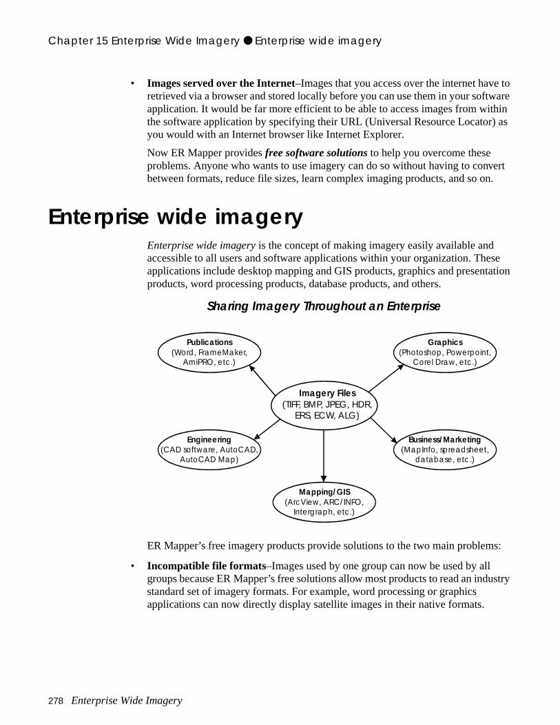
Chapter 15 Enterprise Wide Imagery ● Enterprise wide imagery
to tware thin ) as
vert n.
se tation
s:
ustry
• Images served over the Internet–Images that you access over the internet haveretrieved via a browser and stored locally before you can use them in your sofapplication. It would be far more efficient to be able to access images from withe software application by specifying their URL (Universal Resource Locatoryou would with an Internet browser like Internet Explorer.
Now ER Mapper provides free software solutions to help you overcome these problems. Anyone who wants to use imagery can do so without having to conbetween formats, reduce file sizes, learn complex imaging products, and so o
Enterprise wide imageryEnterprise wide imagery is the concept of making imagery easily available and accessible to all users and software applications within your organization. Theapplications include desktop mapping and GIS products, graphics and presenproducts, word processing products, database products, and others.
ER Mapper’s free imagery products provide solutions to the two main problem
• Incompatible file formats–Images used by one group can now be used by all groups because ER Mapper’s free solutions allow most products to read an indstandard set of imagery formats. For example, word processing or graphics applications can now directly display satellite images in their native formats.
Sharing Imagery Throughout an Enterprise
Imagery Files(TIFF, BMP, JPEG, HDR,
ERS, ECW, ALG)
Engineering(CAD software, AutoCAD,
AutoCAD Map)
Graphics(Photoshop, Powerpoint,
Corel Draw, etc.)
Publications(Word, FrameMaker,
AmiPRO, etc.)
Mapping/GIS(ArcView, ARC/INFO,
Intergraph, etc.)
Business/Marketing(MapInfo, spreadsheet,
database, etc.)
278 Enterprise Wide Imagery
Chapter 15 Enterprise Wide Imagery ● ER Mapper free imagery solutions
ge ple, an
w
ise.
mat
ms.
y
e
s ).
s to sing ,
in you
• Large file sizes–ER Mapper’s free solutions allow your applications to read imafiles of virtually any size very quickly. Mosaics of aerial photographs, for examoften require 100’s of megabytes (even gigabytes) of disk space. ER Mapper’ssolutions handle the underlying technology, so even simple word processors cdisplay very large image files in a snap.
• Images served over the internet–ER Mapper 6.1 allows you to directly access images served over the internet by specifying their URL. The free plug-ins allomost other GIS and Office products to do the same.
ER Mapper free imagery solutionsER Mapper’s free Enterprise Wide Imagery solutions are tightly integrated software tools and plug-ins that let you share images throughout your enterpr
• ER Viewer–A free image viewer that lets you view ER Mapper images and algorithms, TIFF and GeoTIFF files, Windows BMP, JPEG, Universal Data For(UDF), ESRI BIL, and SPOTView image formats.
• Imagery plug-in for Office users–Users of office products (word processing, graphics, spreadsheets, etc.) can use ER Viewer’s OLE capabilities to directlydisplay large imagery files quickly within their applications.
• ER Mapper Imagery Extension for ArcView GIS–A free extension that lets ArcView GIS users display ER Mapper format images and smart data algorith
• MapImagery plug-in for MapInfo –A free plug-in that lets MapInfo users displaand enhance the same image formats supported by ER Viewer.
• AutoCAD Map plug-in –A free plug-in that lets AutoCAD Map users display thsame image formats supported by ER Viewer.
• Autodesk World imagery viewer–Autodesk World lets users display any imagesupported by ER Viewer (this functionality is embedded in the World software
Using ER Mapper for imagingBy using the plug-ins and tools in conjunction with ER Mapper, you gain accesthe powerful capabilities of this leading integrated mapping and image procesapplication. ER Mapper can be used as a central depository for all image datawhere it can be processed as needed before passing on to other applicationsorganization via the plug-ins and tools.
Adding ER Mapper to your enterprise gives you capabilities to:
• Import and display over 100 different image formats
Enterprise Wide Imagery 279
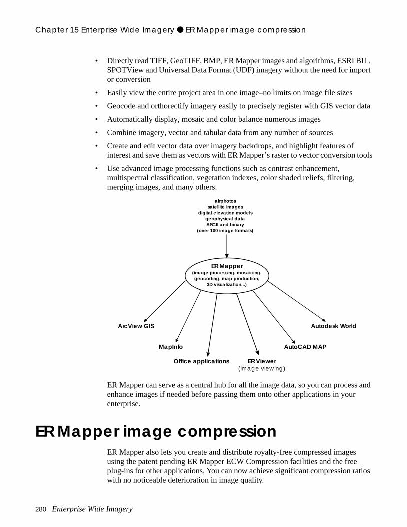
Chapter 15 Enterprise Wide Imagery ● ER Mapper image compression
IL, port
data
n tools
ss and r
s tios
• Directly read TIFF, GeoTIFF, BMP, ER Mapper images and algorithms, ESRI BSPOTView and Universal Data Format (UDF) imagery without the need for imor conversion
• Easily view the entire project area in one image–no limits on image file sizes
• Geocode and orthorectify imagery easily to precisely register with GIS vector
• Automatically display, mosaic and color balance numerous images
• Combine imagery, vector and tabular data from any number of sources
• Create and edit vector data over imagery backdrops, and highlight features ofinterest and save them as vectors with ER Mapper’s raster to vector conversio
• Use advanced image processing functions such as contrast enhancement, multispectral classification, vegetation indexes, color shaded reliefs, filtering, merging images, and many others.
ER Mapper can serve as a central hub for all the image data, so you can proceenhance images if needed before passing them onto other applications in youenterprise.
ER Mapper image compressionER Mapper also lets you create and distribute royalty-free compressed imageusing the patent pending ER Mapper ECW Compression facilities and the freeplug-ins for other applications. You can now achieve significant compression rawith no noticeable deterioration in image quality.
ER Mapper(image processing, mosaicing,geocoding, map production,
3D visualization...)
ER Viewer(image viewing)
Office applications
ArcView GIS
MapInfo
Autodesk World
AutoCAD MAP
airphotossatellite images
digital elevation modelsgeophysical dataASCII and binary
(over 100 image formats)
280 Enterprise Wide Imagery
Chapter 15 Enterprise Wide Imagery ● Working with large images
and mple,
ver
Working with large imagesWhen working with satellite imagery, airphotos, scanned topographical maps other types of imagery, the size of image files can become very large. For exait takes 3 terrabytes (3,000GB) of color imagery to take aerial photographs of typical city at 3 inch resolution. It takes 1.5TB (1,500GB) of color imagery to coall of California at a resolution of one meter.
Compression of imagery offers several advantages including:
• reduced image file size
• faster access
• easier distribution
• the ability to work with imagery covering larger areas
Enterprise Wide Imagery 281

Chapter 15 Enterprise Wide Imagery ● Working with large images
282 Enterprise Wide Imagery

that
e
ats,
16
Using ER ViewerThis chapter explains how to use the free ER Viewer application to display andanalyze several types of image files. ER Viewer is a free Windows application can be installed from the ER Mapper installation CD-ROM or downloaded fromthe ER Mapper website at www.ermapper.com.
About ER ViewerER Viewer is a free, easy to use image viewing application featuring interactivroaming and zooming of very large image files. It also acts as an OLE server application to let you view images inside your favorite Windows applications. ER Viewer offers unequalled stability and supports a wide range of image formincluding:
• Universal Data Format (UDF) images
• ER Mapper compressed and uncompressed images
• TIFF and GeoTIFF images
• Windows BMP images
• SPOTView images
• ESRI BIL (ARC/INFO and ArcView) images
• Smart Data ER Mapper algorithms
Enterprise Wide Imagery 283
Chapter 16 Using ER Viewer ● Hands-on exercises
rform
ata.
Hands-on exercisesThese exercises show you how to use ER Viewer to display image files and pezooming, roaming and measuring distances.
• Use ER Viewer to display images in several different formats
• Interactively zoom and roam images
• View geographic coordinates and measure distances on an image
• Print an image (optional)
Note: The following examples use image files supplied with ER Mapper as sample dIf it is not possible to install ER Mapper, you must have a sample TIFF or BMPimage file to use for the exercises.
1: Using ER Viewer to display images
Start ER Viewer
1 Start ER Viewer by double-clicking the icon on your desktop or selecting Start/Programs/ER Mapper/ER Viewer .
ER Viewer starts up and displays the Getting Started information dialog that contains basic instructions for using ER Viewer.
2 Click Close on the Getting Started With ER Viewer dialog.
3 Click the Maximize button in the upper-right corner of the ER Viewer window (if it is not already maximized)
What you will learn...
After completing these exercises, you will know how to perform the following tasks in ER Viewer and OLE-enabled Windows applications:
Before you begin...
Before beginning these exercises, you must have installed ER Viewer on yoursystem. You can download it free of charge from the ER Mapper web site at www.ermapper.com if needed.
Objectives Learn how to use ER Viewer to display images, zoom and roam around the images, and measure distances on geocoded images.
284 Enterprise Wide Imagery
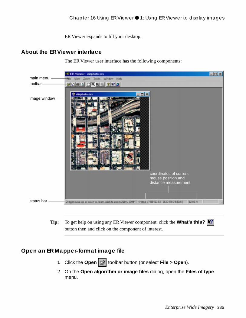
Chapter 16 Using ER Viewer ● 1: Using ER Viewer to display images
ER Viewer expands to fill your desktop.
About the ER Viewer interfaceThe ER Viewer user interface has the following components:
Tip: To get help on using any ER Viewer component, click the What’s this?
button then and click on the component of interest.
Open an ER Mapper-format image file
1 Click the Open toolbar button (or select File > Open ).
2 On the Open algorithm or image files dialog, open the Files of type menu.
coordinates of currentmouse position anddistance measurement
status bar
main menu
toolbar
image window
Enterprise Wide Imagery 285
Chapter 16 Using ER Viewer ● 1: Using ER Viewer to display images
P,
his
g an
ease
A list of image formats supported by ER Viewer displays. You can open ER Mapper-format images and algorithms, graphics formats like TIFF and BMsatellite image formats such as GeoSPOT and ESRI BIL, and others.
3 Select the All image files option.
4 Navigate to the directory where ER Mapper is installed. Open the ‘examples\Shared_Data’ directory. Double-click on the file ‘airphoto.ers.’
ER Viewer displays an aerial photograph of the San Diego, California area. (Tfile was previously imported and saved in ER Mapper ‘.ers’ image file format.)
Note: If the ER Mapper sample data is not installed, navigate to a directory containinimage in TIFF, BMP or other supported format an open it instead.
Enlarge the image window1 Drag the image window by a corner to make it larger.
2 From the Zoom menu, select Data Extents .
The image expands to fill the new image window size.
Use the Zoom Tool to zoom freely in and out
1 Click the Zoom Tool button on the toolbar (or press F6).
2 Point to the center of the image, then drag downward to zoom in.
3 Point to the center of the image, then drag upward to zoom out.
By dragging up or down, you can zoom in or out by any amount. When you relthe mouse, ER Viewer refreshes the image detail as needed.
Use the Zoom Tool to zoom by fixed amounts1 From the Zoom menu, select Data Extents .
The airphoto image zooms out to show the entire image extents.
2 Click on the center of the image to zoom in.
The image zooms in to twice (200%) the previous magnification.
3 While holding down the Ctrl key, click the image center again.
The image zooms out to half (50%) of the previous magnification. With the Zoom
Tool selected, clicking zooms in and Ctrl-clicking zooms out by fixed
amounts.
286 Enterprise Wide Imagery
Chapter 16 Using ER Viewer ● 1: Using ER Viewer to display images
right
map mn
Use the Zoom Box Tool to zoom on an exact area1 From the Zoom menu, select Data Extents .
The image zooms out to show the entire image extents.
2 Click the ZoomBox Tool button (or press F5).
3 Drag a box around the central portion of the image.
ER Viewer zooms in to display the area you defined with your box. Use the ZoomBox Tool tool to zoom in on an exact area of interest.
Use the Hand Tool to roam around (pan) the image
1 Click the Hand Tool button (or press F7).
2 Drag the airphoto within the image window.
ER Viewer roams (or pans) to display the adjacent area of the image. Use the Hand Tool tool to roam around and quickly view adjacent areas of the image.
Tip: When the Zoom Tool is selected, pressing Shift temporarily enables the
Hand Tool .
View geographic locations on the image1 Without depressing the mouse, point to different locations on the image.
The geographic locations of the current mouse position are shown in the lowerpart of the ER Viewer window. (Locations are shown in the units of the map projection. This airphoto is registered to the UTM coordinate system, so the locations are in meters of Easting and Northings.)
Note: Geographic locations only display when your image has been registered to a projection. If your image in unregistered, the locations appear as row and colu(cell) values instead.
Use the Measure Tool to measure distances in the image
1 Click the Measure Tool button (or press F8).
Enterprise Wide Imagery 287
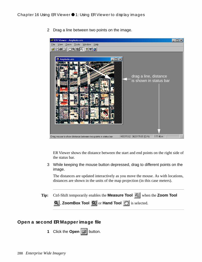
Chapter 16 Using ER Viewer ● 1: Using ER Viewer to display images
ide of
tions,
2 Drag a line between two points on the image.
ER Viewer shows the distance between the start and end points on the right sthe status bar.
3 While keeping the mouse button depressed, drag to different points on the image.
The distances are updated interactively as you move the mouse. As with locadistances are shown in the units of the map projection (in this case meters).
Tip: Ctrl-Shift temporarily enables the Measure Tool when the Zoom Tool
, ZoomBox Tool or Hand Tool is selected.
Open a second ER Mapper image file
1 Click the Open button.
drag a line, distanceis shown in status bar
288 Enterprise Wide Imagery
Chapter 16 Using ER Viewer ● 1: Using ER Viewer to display images
st of on.
new n red
ion
on e
tion
2 Navigate to the directory where ER Mapper is installed. Open the directory ‘examples\Applications\Land_Information.’
Tip: The ‘Automatically adjust contrast on dataset load’ option enhances the contraany image you open automatically. You should usually leave this option turned
3 Double-click on the file ‘SPOT_XS_07Aug88.ers’ to display it.
ER Viewer displays a SPOT XS satellite of the San Diego, California area in aimage window. This is a color infrared image, so vegetated areas are shown itones.
4 Make the image window two times larger, then select Zoom > Data Extents .
5 Zoom in to an area of interest using the Zoom Tool or ZoomBox Tool
.
6 Pan or scroll the image as desired using Hand Tool .
View properties of the image file1 From the View menu, select Properties .
ER Viewer displays tab pages showing properties of the image file.
2 On the Properties dialog, click the Registration tab.
The geodetic datum, map projection, units and other georeferencing informatabout the image file is shown.
3 Click Cancel on the Properties dialog.
Preview a hardcopy print of the image
1 Click the Print Preview button.
ER Viewer redisplays the image to show how it would be sized and positionedyour default printer. ER Viewer tries to center the image on the page and fill thprintable area.
Tip: Only the area you zoomed into will be printed, so you can easily print any porof a large image.
Enterprise Wide Imagery 289
Chapter 16 Using ER Viewer ● 1: Using ER Viewer to display images
er,
in
2 Click Close or click the button on the image window.
The image redisplays in normal mode for zooming and roaming.
Print of the image (optional)
1 Click the Print button.
The Windows Print dialog for your default printer opens to let you select a printchange the properties, and print the image.
2 If desired, select the printer and properties, then click OK to print the image. Otherwise click Cancel to close the Print dialog.
Close ER Viewer
1 Click the Close button on the ER Viewer window (or select File > Exit ).
• Use ER Viewer to display images in several different formats
• Interactively zoom and roam images
• View geographic coordinates and measure distances on an image
• Print an image (optional)
What you learned
After completing these exercises, you know how to perform the following tasksER Viewer:
290 Enterprise Wide Imagery

to out
wer ou t
17
Office applications(OLE)
This chapter explains how you can use your office software’s OLE capabilitieseasily display and manipulate large images inside Windows applications (withhaving to save the image as part of the file).
Note: To use the OLE capabilities described here, make sure you first install ER Vieand perform the exercises in the previous chapter to become familiar with it. Ycan install ER Viewer from the ER Mapper installation CD-ROM or download ifrom the ER Mapper website at www.ermapper.com.
Enterprise Wide Imagery 291
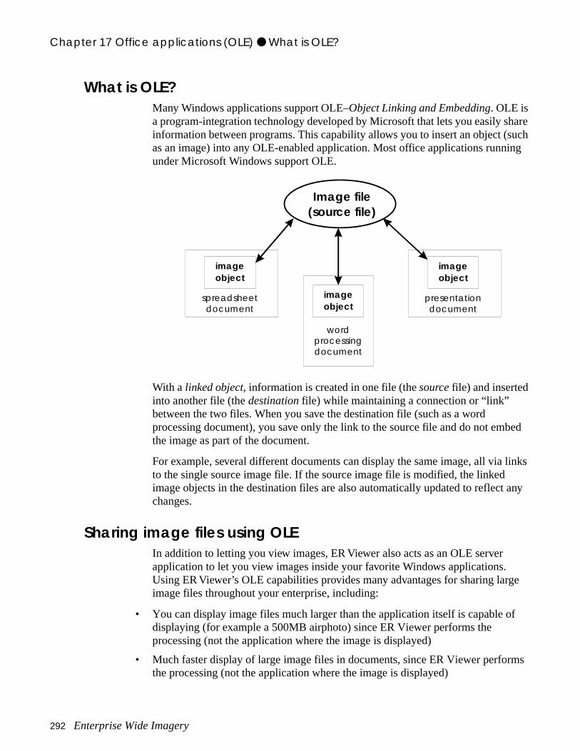
Chapter 17 Office applications (OLE) ● What is OLE?
hare uch ng
bed
links
any
ge
of
ms
What is OLE?Many Windows applications support OLE–Object Linking and Embedding. OLE is a program-integration technology developed by Microsoft that lets you easily sinformation between programs. This capability allows you to insert an object (sas an image) into any OLE-enabled application. Most office applications runniunder Microsoft Windows support OLE.
With a linked object, information is created in one file (the source file) and inserted into another file (the destination file) while maintaining a connection or “link” between the two files. When you save the destination file (such as a word processing document), you save only the link to the source file and do not emthe image as part of the document.
For example, several different documents can display the same image, all viato the single source image file. If the source image file is modified, the linked image objects in the destination files are also automatically updated to reflect changes.
Sharing image files using OLEIn addition to letting you view images, ER Viewer also acts as an OLE server application to let you view images inside your favorite Windows applications. Using ER Viewer’s OLE capabilities provides many advantages for sharing larimage files throughout your enterprise, including:
• You can display image files much larger than the application itself is capable displaying (for example a 500MB airphoto) since ER Viewer performs the processing (not the application where the image is displayed)
• Much faster display of large image files in documents, since ER Viewer perforthe processing (not the application where the image is displayed)
Image file(source file)
spreadsheetdocument
imageobject
wordprocessingdocument
imageobject
presentationdocument
imageobject
292 Enterprise Wide Imagery
Chapter 17 Office applications (OLE) ● Hands-on exercises
ns can
ed by
bed mall in
plex
ation
ata.
• Word processing documents, spreadsheets, presentations, and other applicatioall share a single copy of the original imagery files
• Documents can display images in many additional image formats not supportthe destination application, but that are supported by ER Viewer
• Images can be displayed in the application without having to permanently emand save the image files as part of the document (so the documents remain ssize)
• You can access the power of ER Mapper Smart Data Algorithms to apply comprocessing enhancements that create beautiful images interactively without changing the original image files
Hands-on exercisesThese exercises show you how to insert an image into another Windows applicas a linked OLE object using ER Viewer as the source application.
• Insert an image as a linked OLE object into another Windows application
• Edit the image object within the application using the ER Viewer toolbar
• Copy and paste an OLE image form one area to another
Note: The following examples use image files supplied with ER Mapper as sample dIf it is not possible to install ER Mapper, you must have a sample TIFF or BMPimage file to use for the exercises.
What you will learn...
After completing these exercises, you will know how to perform the following tasks in OLE-enabled Windows applications:
Before you begin...
Before beginning these exercises, you must have installed ER Viewer on yoursystem.
Enterprise Wide Imagery 293
Chapter 17 Office applications (OLE) ● 1: Using OLE to display images
ssing at full
rful uch
if
1: Using OLE to display images
In the past, it was usually necessary to embed large image files in word procedocuments, spreadsheets or presentations in order to display and print them resolution. Since the image file was saved as part of the document, it createdvery large document files and the data could not be edited once it was inserted.
With Object Linking and Embedding (OLE), you can use ER Viewer as a poweimage viewing engine to display and edit large image files directly inside yourWindows applications. This allows you to display images in many formats thatcannot be read by the application itself, and also makes the document files msmaller because only a link to the image file is saved with the document.
The following example uses Microsoft Word as the example OLE-enabled application. You can use any other OLE-enabled word processing application desired (WordPerfect, Framemaker, and so on).
Start Microsoft Word (or other OLE-enabled word processor)1 Start up the Word application on your system (or another OLE-enabled
word processor).
2 Type the text San Diego Airphoto as the first line of your document, then press Enter to create a new line.
Open the Windows Explorer1 Open the Windows Explorer application (select Start > Programs >
Windows Explorer ).
2 Open the ER Mapper installation directory. Then open the directory ‘examples\Applications\Airphoto\1_Geocoding.’
You should see a list of files beginning with ‘San_Diego_Airphoto.’
3 Move the Word application window and the Explorer window side by side (resize them if needed).
Objectives Learn how to use ER Viewer as an OLE server to display and edit large imagefiles within OLE-enabled Windows applications.
294 Enterprise Wide Imagery
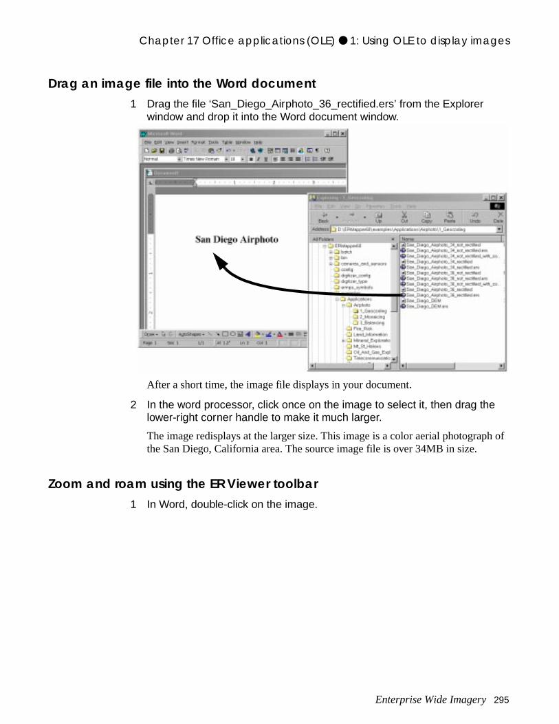
Chapter 17 Office applications (OLE) ● 1: Using OLE to display images
h of
Drag an image file into the Word document1 Drag the file ‘San_Diego_Airphoto_36_rectified.ers’ from the Explorer
window and drop it into the Word document window.
After a short time, the image file displays in your document.
2 In the word processor, click once on the image to select it, then drag the lower-right corner handle to make it much larger.
The image redisplays at the larger size. This image is a color aerial photograpthe San Diego, California area. The source image file is over 34MB in size.
Zoom and roam using the ER Viewer toolbar1 In Word, double-click on the image.
Enterprise Wide Imagery 295
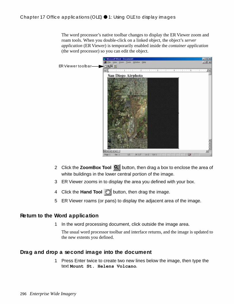
Chapter 17 Office applications (OLE) ● 1: Using OLE to display images
nd
ted to
The word processor’s native toolbar changes to display the ER Viewer zoom aroam tools. When you double-click on a linked object, the object’s server application (ER Viewer) is temporarily enabled inside the container application (the word processor) so you can edit the object.
2 Click the ZoomBox Tool button, then drag a box to enclose the area of white buildings in the lower central portion of the image.
3 ER Viewer zooms in to display the area you defined with your box.
4 Click the Hand Tool button, then drag the image.
5 ER Viewer roams (or pans) to display the adjacent area of the image.
Return to the Word application1 In the word processing document, click outside the image area.
The usual word processor toolbar and interface returns, and the image is updathe new extents you defined.
Drag and drop a second image into the document1 Press Enter twice to create two new lines below the image, then type the
text Mount St. Helens Volcano .
ER Viewer toolbar
296 Enterprise Wide Imagery
Chapter 17 Office applications (OLE) ● 1: Using OLE to display images
after from e
relief
m und
thod
2 In the Explorer window, open the ER Mapper home directory, then open the directory examples\Applications\Mt_St_Helens.
3 Drag the file ‘2D_after_eruption.alg’ from the Explorer window and drop it into the word processing document window.
After a short time, the image file displays in your document.
4 Click once on the image to select it, then drag the lower-right corner handle to make it larger.
This is an image of the Mount St. Helens Volcano in the state of Oregon, USA an eruption that blew out the central portion of the mountain. The image data which this is created is a Digital Elevation Model (DEM) where each pixel valurepresents a terrain elevation. The special processing technique is called a “colordrape” that combines a color image that shows elevation with a shaded image that shows terrain features.
In this case, the image file you linked to is an ER Mapper Smart Data Algorith(.alg). The algorithm file runs the ER Mapper processing engine in the backgroto interactively create the enhanced colordrape image from the original DEM image data.
Tip: Most OLE-enabled applications also let you insert a linked OLE object into a document using a menu command (as an alternative to the drag and drop meshown in the previous example).
Zoom into and center the volcano image1 Double-click on the inserted image to display the ER Viewer toolbar.
Enterprise Wide Imagery 297
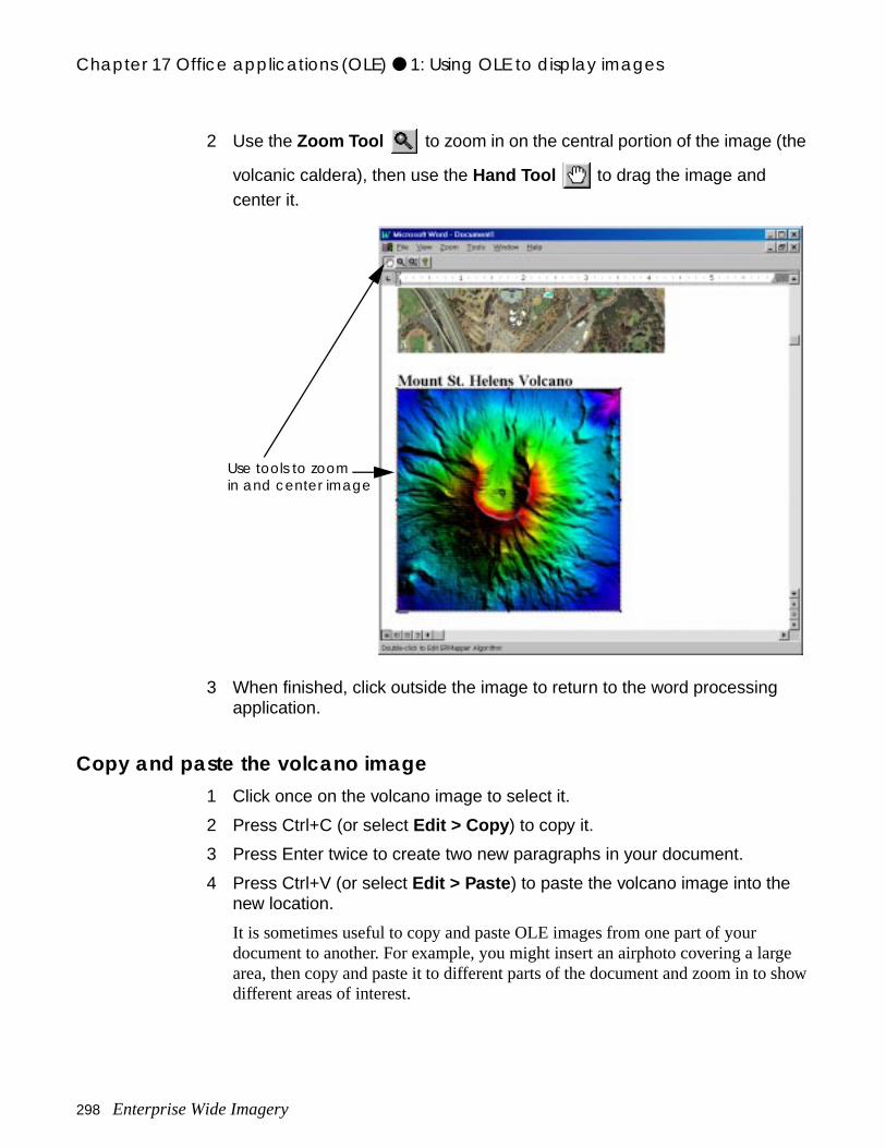
Chapter 17 Office applications (OLE) ● 1: Using OLE to display images
rge show
2 Use the Zoom Tool to zoom in on the central portion of the image (the
volcanic caldera), then use the Hand Tool to drag the image and center it.
3 When finished, click outside the image to return to the word processing application.
Copy and paste the volcano image1 Click once on the volcano image to select it.
2 Press Ctrl+C (or select Edit > Copy ) to copy it.
3 Press Enter twice to create two new paragraphs in your document.
4 Press Ctrl+V (or select Edit > Paste ) to paste the volcano image into the new location.
It is sometimes useful to copy and paste OLE images from one part of your document to another. For example, you might insert an airphoto covering a laarea, then copy and paste it to different parts of the document and zoom in todifferent areas of interest.
Use tools to zoomin and center image
298 Enterprise Wide Imagery
Chapter 17 Office applications (OLE) ● 1: Using OLE to display images
0MB arge em is
in
(Optional) Save your word processing document.1 Save your document, then close the application.
Note: If you check the file size of your word processing document, it should only be about 1MB. Yet this document displays images that are created from almost 4of image files. This is one of the big advantages of OLE–you can display very limage files inside a document very quickly without having to embed the imagefiles. (That is, images are not saved as part of the document, only the link to thsaved.)
• Insert an image as a linked OLE object into another Windows application
• Edit the image object within the application using the ER Viewer toolbar
• Copy and paste an OLE image from one area to another
What you learned
After completing these exercises, you know how to perform the following tasksOLE-enabled Windows applications:
Enterprise Wide Imagery 299

Chapter 17 Office applications (OLE) ● 1: Using OLE to display images
300 Enterprise Wide Imagery

sing
and
apper
ed to e r n,
18
ArcView GISUsers
This chapter explains how to use the free ER Mapper Imagery Extension for ESRI’s ArcView GIS software. It also explains how to obtain and install the extension, and the additional imaging capabilities ArcView users can gain by uthe extension in conjunction with ER Mapper.
Note: You must have a licensed copy of ArcView GIS version 3.1 or greater to installrun the ER Mapper Imagery Extension. You do not need to have a copy of ER Mapper installed, but this is recommended to gain access to sample ER Mimagery and algorithms used in the following tutorial. (You can order the free ER Mapper installation CD-ROM from www.ermapper.com.)
About the ER Mapper Extension for ArcView GISAs imagery data sources become more important for GIS applications, the neefficiently process, enhance and display large image files also becomes moreimportant. Earth Resource Mapping (developers of ER Mapper) provides a freextension (or “plug-in”) that lets ArcView GIS users directly display ER Mappeimagery and algorithms. With the ER Mapper Imagery Extension, ArcView GISusers are no longer restricted by limited image handling capabilities. In additio
Enterprise Wide Imagery 301
Chapter 18 ArcView GIS Users ● Using the extension with ER Mapper
w age
in age
IL, port
data
n tools
ded a and
n
you can experience the full power of ER Mapper algorithms from within ArcVieGIS, and give your vector GIS data real world meaning by presenting it over imbackdrops.
Using the extension with ER MapperBy using the extension in conjunction with ER Mapper, ArcView GIS users gaaccess to the extensive capabilities of this powerful integrated mapping and improcessing software, including:
• Import and display over 100 different image formats
• Directly read TIFF, GeoTIFF, BMP, ER Mapper images and algorithms, ESRI BSPOTView and Universal Data Format (UDF) imagery without the need for imor conversion
• Easily view the entire project area in one image–no limits on image file sizes
• Geocode and orthorectify imagery easily to precisely register with GIS vector
• Automatically display, mosaic and color balance numerous images
• Combine imagery, vector and tabular data from any number of sources
• Create and edit vector data over imagery backdrops, and highlight features ofinterest and save them as vectors with ER Mapper’s raster to vector conversio
• Use advanced image processing functions such as contrast enhancement, multispectral classification, vegetation indexes, color shaded reliefs, filtering, merging images, and many others.
How to obtain the ER Mapper Imagery ExtensionYou can obtain the free ER Mapper Imagery Extension from two sources:
• The ER Mapper installation CD-ROM–The extension can be installed as a separate component from the ER Mapper installation CD-ROM. (It is recommenthat you also install ER Mapper to gain access to a wide variety of sample dattest drive the software in free evaluation mode to see what it can do for you.)
• The ER Mapper web site–You can download the latest version of the extensiofrom the ER Mapper web site at www.ermapper.com. Navigate to the “free software” area and download the ArcView GIS plug-in.
302 Enterprise Wide Imagery
Chapter 18 ArcView GIS Users ● Hands-on exercises
n e
r
Hands-on exercisesThese exercises show you how to use the ER Mapper Imagery extension for ArcView GIS.
• Enable the ER Mapper Imagery Extension after starting ArcView GIS
• Display an ER Mapper image file (.ers) as an Image Data Source
• Display an ER Mapper algorithm file (.alg) as an Image Data Source
• Display a vector theme on an ER Mapper image
1: Using the ER Mapper extension
Start ArcView GIS1 Start the ArcView GIS software on your system.
2 If the Welcome to ArcView GIS dialog appears, click Cancel .
3 Click the Maximize button in the upper-right corner of the ArcView GIS application window (if it is not already maximized)
ArcView GIS expands to fill your desktop.
Load the ER Mapper extension1 From the File menu, select Extensions... .
2 On the Extensions dialog, click on the box next to ‘ER Mapper Algorithms and Imagery’ (a check mark should appear).
What you will learn...
After completing these exercises, you will know how to perform the following tasks in ArcView GIS using the ER Mapper Imagery Extension:
Before you begin...
Before beginning these exercises, you must have installed ArcView GIS versio3.1 or higher and the ER Mapper extension for ArcView on your system. Thesexercises use sample ER Mapper imagery and algorithm files from the ER Mapper installation CD-ROM. You may also follow the general proceduresusing your own ER Mapper imagery (.ers) or algorithm (.alg) files.
Objectives Learn to enable the ER Mapper extension for ArcView and display ER Mappeimagery (.ers) files and algorithm (.alg) files.
Enterprise Wide Imagery 303
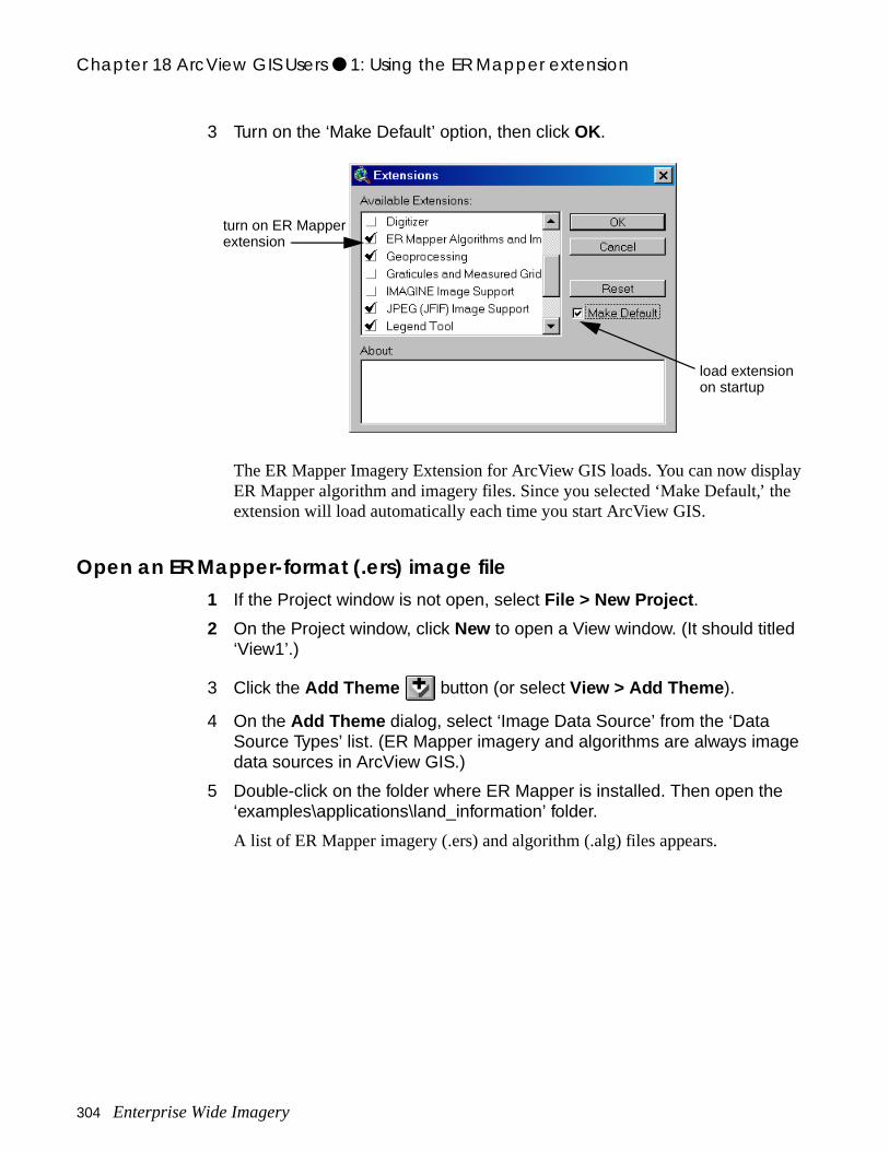
Chapter 18 ArcView GIS Users ● 1: Using the ER Mapper extension
ay e
3 Turn on the ‘Make Default’ option, then click OK.
The ER Mapper Imagery Extension for ArcView GIS loads. You can now displER Mapper algorithm and imagery files. Since you selected ‘Make Default,’ thextension will load automatically each time you start ArcView GIS.
Open an ER Mapper-format (.ers) image file1 If the Project window is not open, select File > New Project .
2 On the Project window, click New to open a View window. (It should titled ‘View1’.)
3 Click the Add Theme button (or select View > Add Theme ).
4 On the Add Theme dialog, select ‘Image Data Source’ from the ‘Data Source Types’ list. (ER Mapper imagery and algorithms are always image data sources in ArcView GIS.)
5 Double-click on the folder where ER Mapper is installed. Then open the ‘examples\applications\land_information’ folder.
A list of ER Mapper imagery (.ers) and algorithm (.alg) files appears.
turn on ER Mapperextension
load extensionon startup
304 Enterprise Wide Imagery
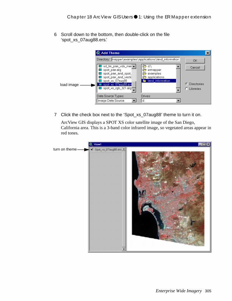
Chapter 18 ArcView GIS Users ● 1: Using the ER Mapper extension
ear in
6 Scroll down to the bottom, then double-click on the file ‘spot_xs_07aug88.ers.’
7 Click the check box next to the ‘Spot_xs_07aug88’ theme to turn it on.
ArcView GIS displays a SPOT XS color satellite image of the San Diego, California area. This is a 3-band color infrared image, so vegetated areas appred tones.
load image
turn on theme
Enterprise Wide Imagery 305
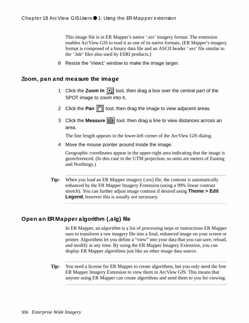
Chapter 18 ArcView GIS Users ● 1: Using the ER Mapper extension
gery to
ge is ting
er en or ad,
free
ing.
This image file is in ER Mapper’s native ‘.ers’ imagery format. The extension enables ArcView GIS to read it as one of its native formats. (ER Mapper’s imaformat is composed of a binary data file and an ASCII header ‘.ers’ file similarthe ‘.hdr’ files also used by ESRI products.)
8 Resize the ‘View1’ window to make the image larger.
Zoom, pan and measure the image
1 Click the Zoom In tool, then drag a box over the central part of the SPOT image to zoom into it.
2 Click the Pan tool, then drag the image to view adjacent areas.
3 Click the Measure tool, then drag a line to view distances across an area.
The line length appears in the lower-left corner of the ArcView GIS dialog.
4 Move the mouse pointer around inside the image.
Geographic coordinates appear in the upper-right area indicating that the imageoreferenced. (In this case to the UTM projection, so units are meters of Easand Northings.)
Tip: When you load an ER Mapper imagery (.ers) file, the contrast is automaticallyenhanced by the ER Mapper Imagery Extension (using a 99% linear contrast stretch). You can further adjust image contrast if desired using Theme > Edit Legend , however this is usually not necessary.
Open an ER Mapper algorithm (.alg) fileIn ER Mapper, an algorithm is a list of processing steps or instructions ER Mappuses to transform a raw imagery file into a final, enhanced image on your screprinter. Algorithms let you define a “view” into your data that you can save, reloand modify at any time. By using the ER Mapper Imagery Extension, you candisplay ER Mapper algorithms just like an other image data source.
Tip: You need a license for ER Mapper to create algorithms, but you only need theER Mapper Imagery Extension to view them in ArcView GIS. This means thatanyone using ER Mapper can create algorithms and send them to you for view
306 Enterprise Wide Imagery
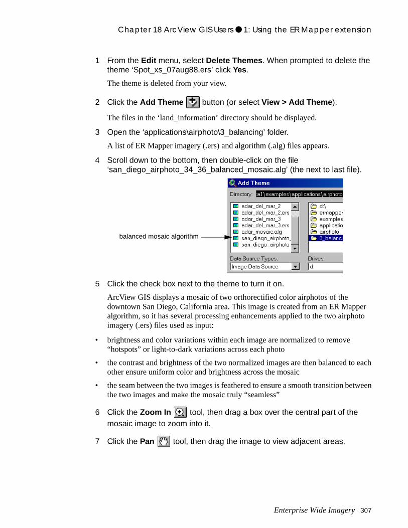
Chapter 18 ArcView GIS Users ● 1: Using the ER Mapper extension
per oto
o each
etween
1 From the Edit menu, select Delete Themes . When prompted to delete the theme ‘Spot_xs_07aug88.ers’ click Yes.
The theme is deleted from your view.
2 Click the Add Theme button (or select View > Add Theme ).
The files in the ‘land_information’ directory should be displayed.
3 Open the ‘applications\airphoto\3_balancing’ folder.
A list of ER Mapper imagery (.ers) and algorithm (.alg) files appears.
4 Scroll down to the bottom, then double-click on the file ‘san_diego_airphoto_34_36_balanced_mosaic.alg’ (the next to last file).
5 Click the check box next to the theme to turn it on.
ArcView GIS displays a mosaic of two orthorectified color airphotos of the downtown San Diego, California area. This image is created from an ER Mapalgorithm, so it has several processing enhancements applied to the two airphimagery (.ers) files used as input:
• brightness and color variations within each image are normalized to remove “hotspots” or light-to-dark variations across each photo
• the contrast and brightness of the two normalized images are then balanced tother ensure uniform color and brightness across the mosaic
• the seam between the two images is feathered to ensure a smooth transition bthe two images and make the mosaic truly “seamless”
6 Click the Zoom In tool, then drag a box over the central part of the mosaic image to zoom into it.
7 Click the Pan tool, then drag the image to view adjacent areas.
balanced mosaic algorithm
Enterprise Wide Imagery 307
Chapter 18 ArcView GIS Users ● 1: Using the ER Mapper extension
to IS.
osaic
a
igh
s at
at d to s of
the the hen
real
This example shows how you can access the power of ER Mapper algorithmsapply complex image enhancements and display them directly with ArcView GThis example uses only two airphotos, but you could just as easily display a malgorithm containing 100’s of megabytes (even gigabytes) of airphoto images.
Add a second view to display a merged satellite image
1 Click the Minimize button on the ‘View1’ window to minimize it (or close it if desired).
2 On the Project window, click New to open a new View window. (It should be titled ‘View2’.)
3 Click the Add Theme button (or select View > Add Theme ).
The files in the ‘3_balancing’ directory should be displayed.
4 Open the ‘examples\functions_and_features\data_fusion’ folder.
A list of ER Mapper algorithm (.alg) files appears. These algorithms all show different ways of merging (or “fusing”) two different images into one.
5 Double-click on the file ‘brovey_transform.alg.’
6 In the ‘View2’ window turn on the ‘Brovey_transform’ theme.
ArcView GIS displays a color image of the San Diego, California area. This ismerge of a Landsat TM satellite image (bands 5, 4 and 2) and a SPOT Panchromatic satellite image. By merging the two types of data, you get the hspatial detail provided by the SPOT Pan image (10-meter resolution) with the multispectral color information provided by the Landsat TM image (seven band30-meter resolution).
The Brovey Transform is a mathematical way of combining the two images thalso greatly enhances the color. Merging or fusion techniques like this are usecombine the strengths of different satellite sensors and create up-to-date viewthe earth’s surface.
7 Enlarge the ‘View2’ window to make the image larger.
8 Zoom in and pan to different parts of the image using the Zoom In and
Pan tools.
The image shows a high resolution, color-enhanced view of the area. As with airphoto mosaic, the ER Mapper algorithm creates this image interactively fromtwo separate Landsat and SPOT satellite imagery files. (The Brovey Transformtechnique usually requires up to three intermediate image files to be created wusing traditional imaging software, but ER Mapper performs the processing intime from the two source images without creating intermediate files.)
308 Enterprise Wide Imagery
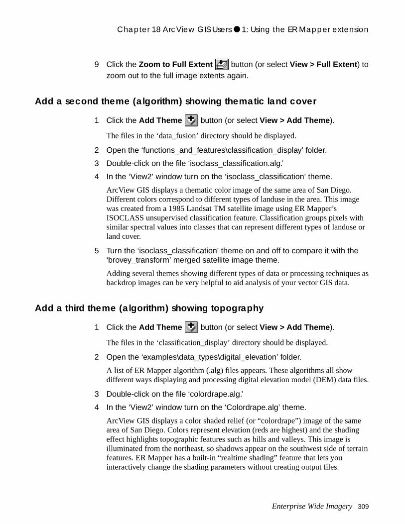
Chapter 18 ArcView GIS Users ● 1: Using the ER Mapper extension
e
ith se or
es as
iles.
e ing
errain
9 Click the Zoom to Full Extent button (or select View > Full Extent ) to zoom out to the full image extents again.
Add a second theme (algorithm) showing thematic land cover
1 Click the Add Theme button (or select View > Add Theme ).
The files in the ‘data_fusion’ directory should be displayed.
2 Open the ‘functions_and_features\classification_display’ folder.
3 Double-click on the file ‘isoclass_classification.alg.’
4 In the ‘View2’ window turn on the ‘isoclass_classification’ theme.
ArcView GIS displays a thematic color image of the same area of San Diego. Different colors correspond to different types of landuse in the area. This imagwas created from a 1985 Landsat TM satellite image using ER Mapper’s ISOCLASS unsupervised classification feature. Classification groups pixels wsimilar spectral values into classes that can represent different types of landuland cover.
5 Turn the ‘isoclass_classification’ theme on and off to compare it with the ‘brovey_transform’ merged satellite image theme.
Adding several themes showing different types of data or processing techniqubackdrop images can be very helpful to aid analysis of your vector GIS data.
Add a third theme (algorithm) showing topography
1 Click the Add Theme button (or select View > Add Theme ).
The files in the ‘classification_display’ directory should be displayed.
2 Open the ‘examples\data_types\digital_elevation’ folder.
A list of ER Mapper algorithm (.alg) files appears. These algorithms all show different ways displaying and processing digital elevation model (DEM) data f
3 Double-click on the file ‘colordrape.alg.’
4 In the ‘View2’ window turn on the ‘Colordrape.alg’ theme.
ArcView GIS displays a color shaded relief (or “colordrape”) image of the samarea of San Diego. Colors represent elevation (reds are highest) and the shadeffect highlights topographic features such as hills and valleys. This image is illuminated from the northeast, so shadows appear on the southwest side of tfeatures. ER Mapper has a built-in “realtime shading” feature that lets you interactively change the shading parameters without creating output files.
Enterprise Wide Imagery 309
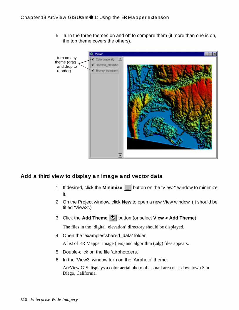
Chapter 18 ArcView GIS Users ● 1: Using the ER Mapper extension
5 Turn the three themes on and off to compare them (if more than one is on, the top theme covers the others).
Add a third view to display an image and vector data
1 If desired, click the Minimize button on the ‘View2’ window to minimize it.
2 On the Project window, click New to open a new View window. (It should be titled ‘View3’.)
3 Click the Add Theme button (or select View > Add Theme ).
The files in the ‘digital_elevation’ directory should be displayed.
4 Open the ‘examples\shared_data’ folder.
A list of ER Mapper image (.ers) and algorithm (.alg) files appears.
5 Double-click on the file ‘airphoto.ers.’
6 In the ‘View3’ window turn on the ‘Airphoto’ theme.
ArcView GIS displays a color aerial photo of a small area near downtown SanDiego, California.
turn on anytheme (dragand drop toreorder)
310 Enterprise Wide Imagery
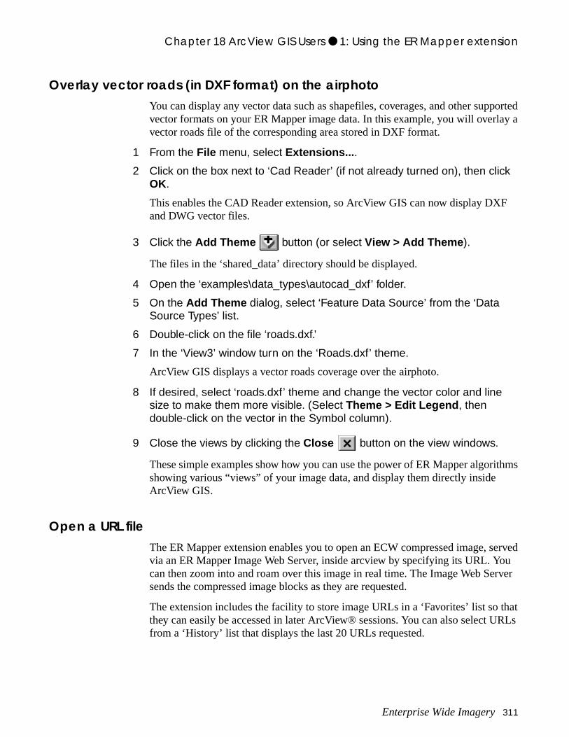
Chapter 18 ArcView GIS Users ● 1: Using the ER Mapper extension
ported ay a
F
ithms
served u rver
that RLs
Overlay vector roads (in DXF format) on the airphotoYou can display any vector data such as shapefiles, coverages, and other supvector formats on your ER Mapper image data. In this example, you will overlvector roads file of the corresponding area stored in DXF format.
1 From the File menu, select Extensions... .
2 Click on the box next to ‘Cad Reader’ (if not already turned on), then click OK.
This enables the CAD Reader extension, so ArcView GIS can now display DXand DWG vector files.
3 Click the Add Theme button (or select View > Add Theme ).
The files in the ‘shared_data’ directory should be displayed.
4 Open the ‘examples\data_types\autocad_dxf’ folder.
5 On the Add Theme dialog, select ‘Feature Data Source’ from the ‘Data Source Types’ list.
6 Double-click on the file ‘roads.dxf.’
7 In the ‘View3’ window turn on the ‘Roads.dxf’ theme.
ArcView GIS displays a vector roads coverage over the airphoto.
8 If desired, select ‘roads.dxf’ theme and change the vector color and line size to make them more visible. (Select Theme > Edit Legend , then double-click on the vector in the Symbol column).
9 Close the views by clicking the Close button on the view windows.
These simple examples show how you can use the power of ER Mapper algorshowing various “views” of your image data, and display them directly inside ArcView GIS.
Open a URL fileThe ER Mapper extension enables you to open an ECW compressed image, via an ER Mapper Image Web Server, inside arcview by specifying its URL. Yocan then zoom into and roam over this image in real time. The Image Web Sesends the compressed image blocks as they are requested.
The extension includes the facility to store image URLs in a ‘Favorites’ list so they can easily be accessed in later ArcView® sessions. You can also select Ufrom a ‘History’ list that displays the last 20 URLs requested.
Enterprise Wide Imagery 311
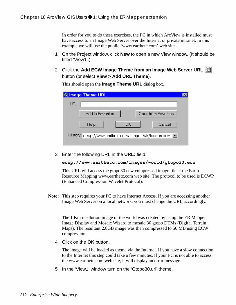
Chapter 18 ArcView GIS Users ● 1: Using the ER Mapper extension
st his
WP
her
tion ess
In order for you to do these exercises, the PC in which ArcView is installed muhave access to an Image Web Server over the Internet or private intranet. In texample we will use the public ‘www.earthetc.com’ web site.
1 On the Project window, click New to open a new View window. (It should be titled ‘View1’.)
2 Click the Add ECW Image Theme from an Image Web Server URL
button (or select View > Add URL Theme ).
This should open the Image Theme URL dialog box.
3 Enter the following URL in the URL: field.
ecwp://www.earthetc.com/images/world/gtopo30.ecw
This URL will access the gtopo30.ecw compressed image file at the Earth Resource Mapping www.earthetc.com web site. The protocol to be used is EC(Enhanced Compression Wavelet Protocol).
Note: This step requires your PC to have Internet Access. If you are accessing anotImage Web Server on a local network, you must change the URL accordingly.
The 1 Km resolution image of the world was created by using the ER MapperImage Display and Mosaic Wizard to mosaic 30 gtopo DTMs (Digital Terrain Maps). The resultant 2.8GB image was then compressed to 50 MB using ECWcompression.
4 Click on the OK button.
The image will be loaded as theme via the Internet. If you have a slow connecto the Internet this step could take a few minutes. If your PC is not able to accthe www.earthetc.com web site, it will display an error message.
5 In the ‘View1’ window turn on the ‘Gtopo30.url’ theme.
312 Enterprise Wide Imagery
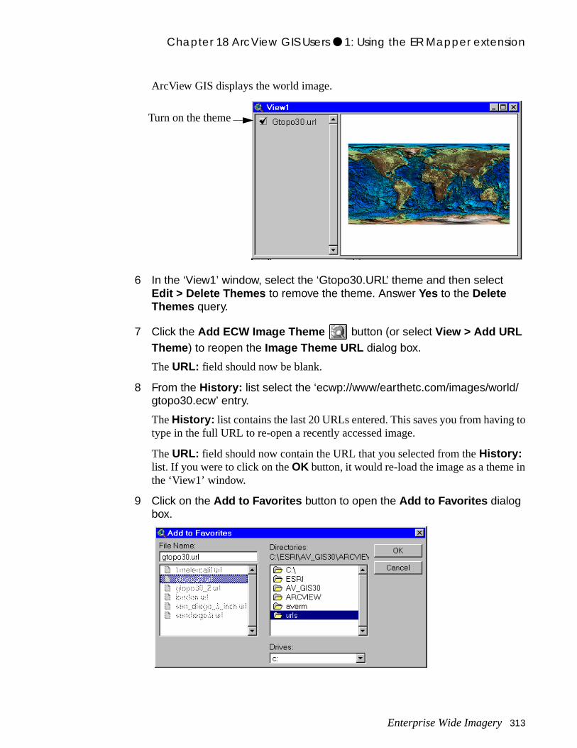
Chapter 18 ArcView GIS Users ● 1: Using the ER Mapper extension
g to
in
ArcView GIS displays the world image.
6 In the ‘View1’ window, select the ‘Gtopo30.URL’ theme and then select Edit > Delete Themes to remove the theme. Answer Yes to the Delete Themes query.
7 Click the Add ECW Image Theme button (or select View > Add URL Theme ) to reopen the Image Theme URL dialog box.
The URL: field should now be blank.
8 From the History: list select the ‘ecwp://www/earthetc.com/images/world/gtopo30.ecw’ entry.
The History: list contains the last 20 URLs entered. This saves you from havintype in the full URL to re-open a recently accessed image.
The URL: field should now contain the URL that you selected from the History: list. If you were to click on the OK button, it would re-load the image as a theme the ‘View1’ window.
9 Click on the Add to Favorites button to open the Add to Favorites dialog box.
Turn on the theme
Enterprise Wide Imagery 313
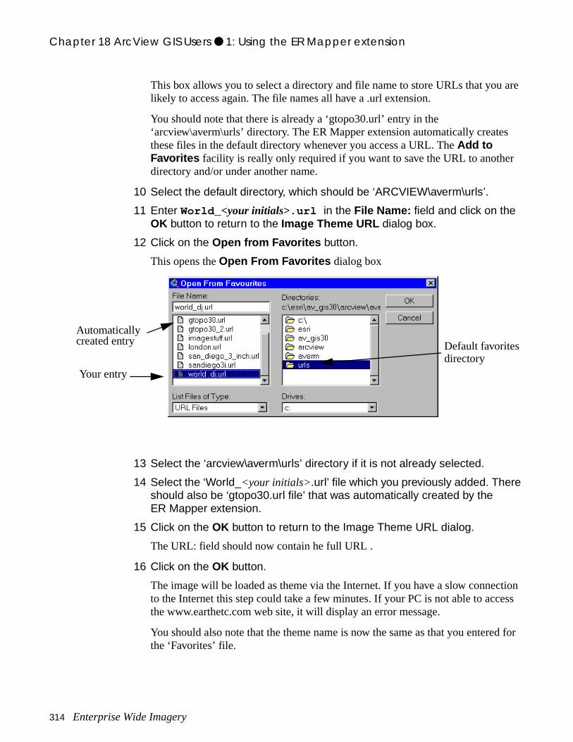
Chapter 18 ArcView GIS Users ● 1: Using the ER Mapper extension
are
s
r
tion ess
d for
This box allows you to select a directory and file name to store URLs that youlikely to access again. The file names all have a .url extension.
You should note that there is already a ‘gtopo30.url’ entry in the ‘arcview\averm\urls’ directory. The ER Mapper extension automatically createthese files in the default directory whenever you access a URL. The Add to Favorites facility is really only required if you want to save the URL to anothedirectory and/or under another name.
10 Select the default directory, which should be ‘ARCVIEW\averm\urls’.
11 Enter World_ <your initials>.url in the File Name: field and click on the OK button to return to the Image Theme URL dialog box.
12 Click on the Open from Favorites button.
This opens the Open From Favorites dialog box
13 Select the ‘arcview\averm\urls’ directory if it is not already selected.
14 Select the ‘World_<your initials>.url’ file which you previously added. There should also be ‘gtopo30.url file’ that was automatically created by the ER Mapper extension.
15 Click on the OK button to return to the Image Theme URL dialog.
The URL: field should now contain he full URL .
16 Click on the OK button.
The image will be loaded as theme via the Internet. If you have a slow connecto the Internet this step could take a few minutes. If your PC is not able to accthe www.earthetc.com web site, it will display an error message.
You should also note that the theme name is now the same as that you enterethe ‘Favorites’ file.
Default favoritesdirectory
Your entry
Automaticallycreated entry
314 Enterprise Wide Imagery
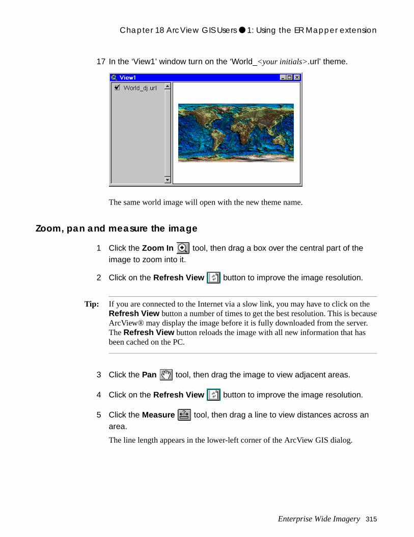
Chapter 18 ArcView GIS Users ● 1: Using the ER Mapper extension
e use
.
17 In the ‘View1’ window turn on the ‘World_<your initials>.url’ theme.
The same world image will open with the new theme name.
Zoom, pan and measure the image
1 Click the Zoom In tool, then drag a box over the central part of the image to zoom into it.
2 Click on the Refresh View button to improve the image resolution.
Tip: If you are connected to the Internet via a slow link, you may have to click on thRefresh View button a number of times to get the best resolution. This is becaArcView® may display the image before it is fully downloaded from the serverThe Refresh View button reloads the image with all new information that has been cached on the PC.
3 Click the Pan tool, then drag the image to view adjacent areas.
4 Click on the Refresh View button to improve the image resolution.
5 Click the Measure tool, then drag a line to view distances across an area.
The line length appears in the lower-left corner of the ArcView GIS dialog.
Enterprise Wide Imagery 315
Chapter 18 ArcView GIS Users ● 1: Using the ER Mapper extension
in
Close ArcView GIS1 If desired, save your views as an ArcView project using File > Save Project
As....
2 Close ArcView GIS by clicking the Close button on the application window or selecting File > Exit .
• Enable the ER Mapper Imagery Extension after starting ArcView GIS
• Display an ER Mapper image file (.ers) as an Image Data Source
• Display an ER Mapper algorithm file (.alg) as an Image Data Source
• Display a vector theme on an ER Mapper image
• Display an ER Mapper URL file (.ecw) as an Image Data Source.
What you learned...
After completing these exercises, you know how to perform the following tasksArcView GIS using the ER Mapper Imagery Extension:
316 Enterprise Wide Imagery

ry ll
run led,
ed to lay sing
port:
s ats
ers.
19
MapInfo UsersThis chapter explains how to use the free MapImagery plug-in for MapInfo software to view ER Mapper imagery and algorithm files. (The free MapImageplug-in is developed by GID Australia.) It also explains how to obtain and instathe plug-in, and the additional imaging capabilities MapInfo users can gain byusing the plug-in in conjunction with ER Mapper.
Note: You must have a licensed copy of MapInfo version 4.5 or greater to install andthe MapImagery plug-in. You do not need to have a copy of ER Mapper instalbut this is recommended to gain access to sample ER Mapper imagery and algorithms used in the following tutorial. (You can order the free ER Mapper installation CD-ROM from www.ermapper.com.)
About the MapImagery plug-in for MapInfoAs imagery data sources become more important for GIS applications, the neefficiently display, process and enhance large image files also becomes moreimportant. GID Australia provides a plug-in that lets MapInfo users directly dispER Mapper imagery and algorithms. This plug-in uses the ER Mapper procesengine to display imagery within MapInfo.
Using the plug-ins, MapInfo users can choose from three levels of imagery sup
• Level 1 (using the free MapImagery plug-in)–By installing the free MapImageryplug-in, MapInfo users can directly display ER Mapper imagery and algorithmfrom within MapInfo. You can also use the plug-in to display other imagery formdirectly supported by ER Mapper such as GeoTIFF, BMP, GeoSPOT and oth
Enterprise Wide Imagery 317
Chapter 19 MapInfo Users ● How to obtain the free MapImagery plug-in
ge
uch
at See
ss the
saics tral /
te to
b d the
te be
fo.
• Level 2 (using the commercial MapImagery plug-in)–By installing the commercial version of MapImagery plug-in, MapInfo users add advanced imaprocessing capabilities to MapInfo. These include contrast enhancement, convolution filtering, image mathematics functions, color lookup tables, and mmore. The commercial version can also create ER Mapper algorithms. For information on the commercial version, contact GID Australia at their web sitewww.gid.com. (GID Australia also makes other ER Mapper and MapInfo tools. their website for information.)
• Level 3 (using the free MapImagery plug-in with a licensed copy of ER Mapper)–By purchasing a license for ER Mapper, MapInfo users can accethe full range of high-level ER Mapper image processing functions, and displayimages within MapInfo using the free or commercial MapImagery plug-in. ER Mapper provides functions for easily creating seamless, color balanced moof many large image files such as airphotos. It also provides advanced imageprocessing functions such as orthorectification, image reprojection, multispecclassification, color shaded reliefs, raster to vector conversion, image mergingfusion, support for over 100 imagery formats and over 200 hardcopy printing devices, and much more.
How to obtain the free MapImagery plug-inYou can obtain the free MapImagery plug-in from three sources:
• The GID Australia web site–GID Australia regularly updates the MapImagery plug-in and posts the latest version on their web site at www.gid.com. Navigathe “products and services” area and download the free MapImagery plug-in.
• The ER Mapper web site–You can download the plug-in from the ER Mapper wesite at www.ermapper.com. Navigate to the “free software” area and downloaMapInfo plug-in.
• The ER Mapper installation CD-ROM–The plug-in can be installed as a separacomponent from the ER Mapper installation CD-ROM. (Note that this may notthe latest version. Check the GID Australia web site for the latest update.)
Hands-on exercisesThese exercises show you how to use the free MapImagery plug-in for MapIn
• Display an ER Mapper image file (.ers) as a MapInfo table
• Display an ER Mapper algorithm file (.alg) as MapInfo table
• Overlay MapInfo vector and tabular table data on an ER Mapper image
What you will learn...
After completing these exercises, you will know how to perform the following tasks in MapInfo using the free MapImagery plug-in:
318 Enterprise Wide Imagery
Chapter 19 MapInfo Users ● 1: Open an ER Mapper image file
the
or
s
• Choose MapImagery setup options to control image display and printing
Note: These exercises use sample ER Mapper imagery and algorithm files from theER Mapper installation CD-ROM. You may also follow the general proceduresusing your own ER Mapper imagery (.ers) or algorithm (.alg) files.
1: Open an ER Mapper image file
Note: You can use the following procedure to open any image formats supported byMapImagery, including TIFF, Windows BMP, JPEG, SPOTView, ESRI BIL, andothers. (Additional formats are added periodically, so make sure you are usinglatest version of MapImagery.)
Start MapInfo1 Start the MapInfo software on your system.
2 If the Quick Start dialog appears, click Cancel on it.
Before you begin...
Before beginning these exercises, you must have installed MapInfo version 4.5higher and the free version of the MapImagery plug-in on your system.
Objectives Learn to use the MapImagery plug-in to display ER Mapper imagery (.ers) fileand to zoom, pan and measure distances on the image.
Enterprise Wide Imagery 319
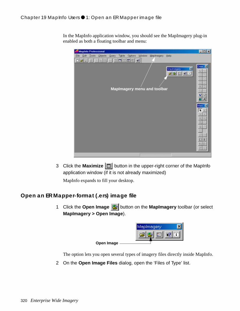
Chapter 19 MapInfo Users ● 1: Open an ER Mapper image file
.
In the MapInfo application window, you should see the MapImagery plug-in enabled as both a floating toolbar and menu:
3 Click the Maximize button in the upper-right corner of the MapInfo application window (if it is not already maximized)
MapInfo expands to fill your desktop.
Open an ER Mapper-format (.ers) image file
1 Click the Open Image button on the MapImagery toolbar (or select MapImagery > Open Image ).
The option lets you open several types of imagery files directly inside MapInfo
2 On the Open Image Files dialog, open the ‘Files of Type’ list.
MapImagery menu and toolbar
Open Image
320 Enterprise Wide Imagery
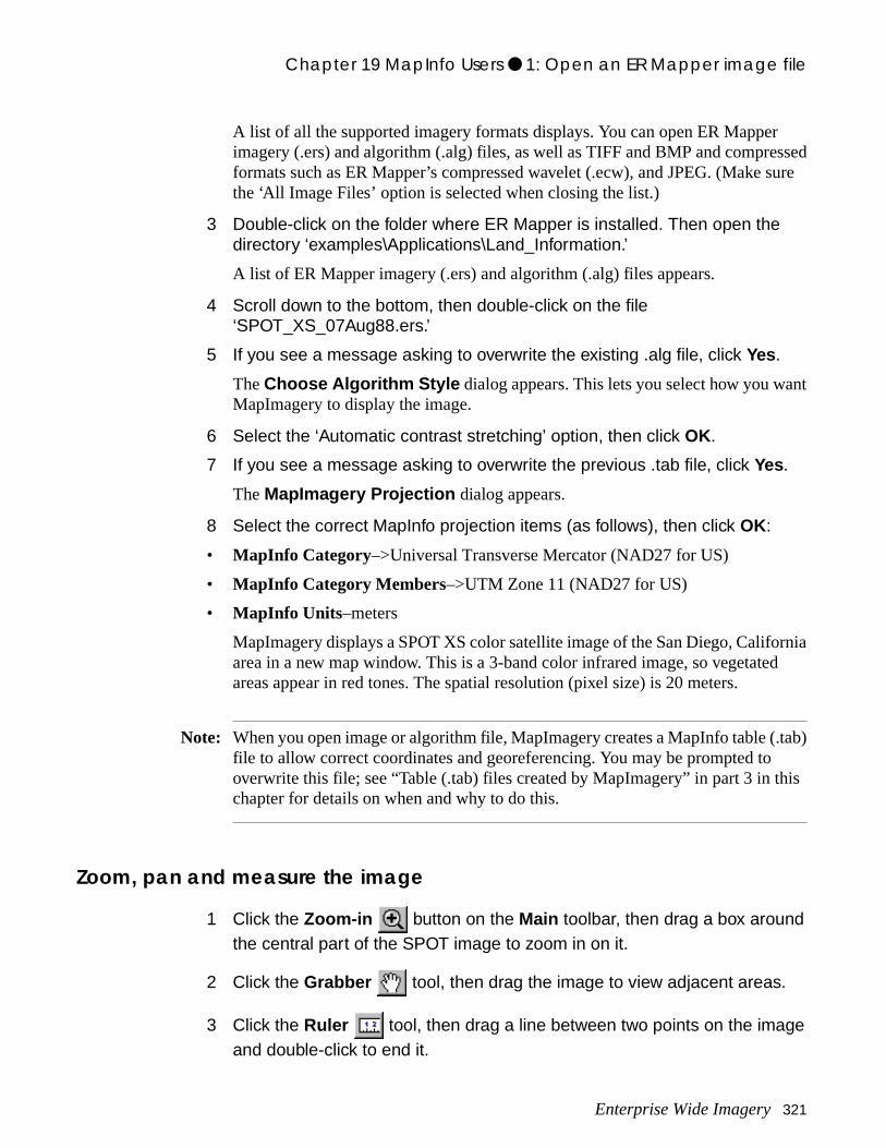
Chapter 19 MapInfo Users ● 1: Open an ER Mapper image file
ssed sure
nt
rnia d
.tab)
is
A list of all the supported imagery formats displays. You can open ER Mapperimagery (.ers) and algorithm (.alg) files, as well as TIFF and BMP and compreformats such as ER Mapper’s compressed wavelet (.ecw), and JPEG. (Make the ‘All Image Files’ option is selected when closing the list.)
3 Double-click on the folder where ER Mapper is installed. Then open the directory ‘examples\Applications\Land_Information.’
A list of ER Mapper imagery (.ers) and algorithm (.alg) files appears.
4 Scroll down to the bottom, then double-click on the file ‘SPOT_XS_07Aug88.ers.’
5 If you see a message asking to overwrite the existing .alg file, click Yes.
The Choose Algorithm Style dialog appears. This lets you select how you waMapImagery to display the image.
6 Select the ‘Automatic contrast stretching’ option, then click OK.
7 If you see a message asking to overwrite the previous .tab file, click Yes.
The MapImagery Projection dialog appears.
8 Select the correct MapInfo projection items (as follows), then click OK:
• MapInfo Category–>Universal Transverse Mercator (NAD27 for US)
• MapInfo Category Members–>UTM Zone 11 (NAD27 for US)
• MapInfo Units –meters
MapImagery displays a SPOT XS color satellite image of the San Diego, Califoarea in a new map window. This is a 3-band color infrared image, so vegetateareas appear in red tones. The spatial resolution (pixel size) is 20 meters.
Note: When you open image or algorithm file, MapImagery creates a MapInfo table (file to allow correct coordinates and georeferencing. You may be prompted to overwrite this file; see “Table (.tab) files created by MapImagery” in part 3 in thchapter for details on when and why to do this.
Zoom, pan and measure the image
1 Click the Zoom-in button on the Main toolbar, then drag a box around the central part of the SPOT image to zoom in on it.
2 Click the Grabber tool, then drag the image to view adjacent areas.
3 Click the Ruler tool, then drag a line between two points on the image and double-click to end it.
Enterprise Wide Imagery 321
Chapter 19 MapInfo Users ● 2: Open ER Mapper algorithm files
inates
er en or ad,
l nto
s,
The distance along the line is displayed in the pop-up Ruler dialog.
4 Select Map > View Entire Layer, then click OK on the pop-up dialog.
The image zooms out to the full extents of the SPOT satellite image.
View geographic coordinates on the image1 Select Map > Options .
2 On the Map Options dialog, select degrees or meters for ‘Coordinate Units’ (whichever you prefer).
3 Under ‘Display in Status Bar,’ click ‘Cursor Location.’ Then click OK.
4 Move the cursor around inside the satellite image.
Geographic coordinates appear in the Status Bar (lower-left area). The coordare in Latitude/Longitude (if you chose degrees) or meters of Eastings and Northings in the UTM projection (if you chose meters).
5 Select File > Close All to close all current tables (in case any others were also open).
2: Open ER Mapper algorithm files
Open an ER Mapper algorithm (.alg) fileIn ER Mapper, an algorithm is a list of processing steps or instructions ER Mappuses to transform a raw imagery file into a final, enhanced image on your screprinter. Algorithms let you define a “view” into your data that you can save, reloand modify at any time. By using the MapImagery plug-in, you can display ER Mapper algorithms just like any other imagery file.
Tip: You can create algorithm files with ER Mapper or with the commerciaversion of the MapImagery plug-in. You only need the free MapImagery plug-iview algorithm files in MapInfo.
Objectives Learn to use the MapImagery plug-in to display ER Mapper algorithm (.alg) fileand to add several images as different layers in your map.
322 Enterprise Wide Imagery
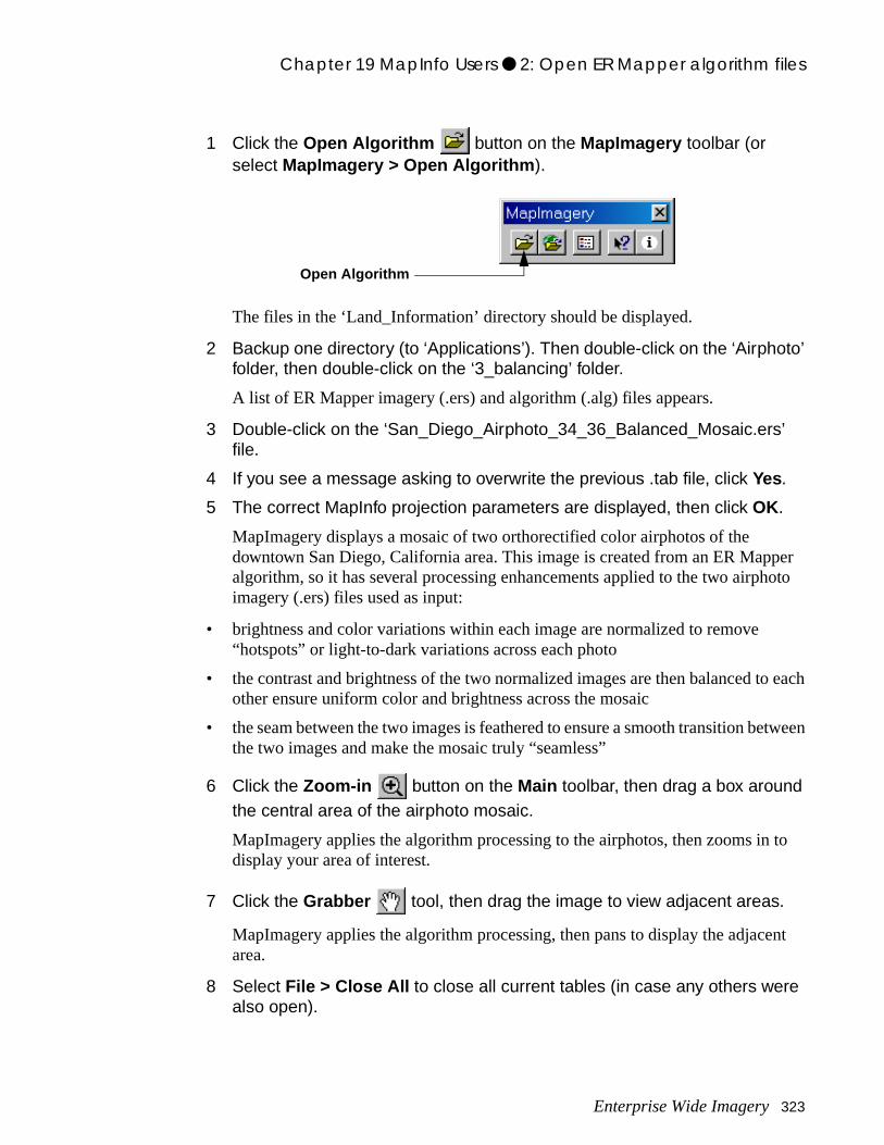
Chapter 19 MapInfo Users ● 2: Open ER Mapper algorithm files
per oto
o each
etween
to
ent
1 Click the Open Algorithm button on the MapImagery toolbar (or select MapImagery > Open Algorithm ).
The files in the ‘Land_Information’ directory should be displayed.
2 Backup one directory (to ‘Applications’). Then double-click on the ‘Airphoto’ folder, then double-click on the ‘3_balancing’ folder.
A list of ER Mapper imagery (.ers) and algorithm (.alg) files appears.
3 Double-click on the ‘San_Diego_Airphoto_34_36_Balanced_Mosaic.ers’ file.
4 If you see a message asking to overwrite the previous .tab file, click Yes.
5 The correct MapInfo projection parameters are displayed, then click OK.
MapImagery displays a mosaic of two orthorectified color airphotos of the downtown San Diego, California area. This image is created from an ER Mapalgorithm, so it has several processing enhancements applied to the two airphimagery (.ers) files used as input:
• brightness and color variations within each image are normalized to remove “hotspots” or light-to-dark variations across each photo
• the contrast and brightness of the two normalized images are then balanced tother ensure uniform color and brightness across the mosaic
• the seam between the two images is feathered to ensure a smooth transition bthe two images and make the mosaic truly “seamless”
6 Click the Zoom-in button on the Main toolbar, then drag a box around the central area of the airphoto mosaic.
MapImagery applies the algorithm processing to the airphotos, then zooms indisplay your area of interest.
7 Click the Grabber tool, then drag the image to view adjacent areas.
MapImagery applies the algorithm processing, then pans to display the adjacarea.
8 Select File > Close All to close all current tables (in case any others were also open).
Open Algorithm
Enterprise Wide Imagery 323
Chapter 19 MapInfo Users ● 2: Open ER Mapper algorithm files
to . o 00’s
tion
per
en a
a
igh
This example shows how you can access the power of ER Mapper algorithmsapply complex image enhancements and display them directly within MapInfo(Each one of these airphotos is over 30MB in size.) This example uses only twairphotos, but you could just as easily display a mosaic algorithm containing 1of megabytes (even gigabytes) of airphoto images.
Note: When you have displayed an image and selected the projection information inMapInfo, MapImagery remembers this in the future. See “Choosing map projecinformation” in part 3 in this chapter for more information on how and when toselect projections.
Set the option to add multiple images to the current mapperFor this next example, you will add several images as layers in the same mapwindow. MapImagery has setup options to make this easier.
1 Click the MapImagery Options button (on the MapImagery toolbar), or select MapImagery > MapImagery Options .
2 Click the General tab. Under ‘When Opening an Algorithm Table’ select the ‘Add to Current Mapper’ option. Click OK.
This tells MapImagery to add new images to the same mapper, rather than opnew mapper each time.
Open a merged satellite image algorithm
1 Click the Open Algorithm button on the MapImagery toolbar (or select MapImagery > Open Algorithm ).
The files in the ‘3_Balancing’ directory should be displayed.
2 Backup to the ‘examples’ directory. Double-click on the ‘Functions_and_Features’ folder, then double-click on the ‘Data_Fusion’ folder.
A list of ER Mapper algorithm (.alg) files appears. These algorithms all show different ways of merging (or “fusing”) two different images into one.
3 Double-click on the file ‘Brovey_Transform.alg.’
4 The correct MapInfo projection parameters are displayed, then click OK.
MapImagery displays a color image of the San Diego, California area. This is merge of a Landsat TM satellite image (bands 5, 4 and 2) and a SPOT Panchromatic satellite image. By merging the two types of data, you get the h
324 Enterprise Wide Imagery
Chapter 19 MapInfo Users ● 2: Open ER Mapper algorithm files
s at
at d to date
en
the the hen
real
e
ith se or
spatial detail provided by the SPOT Pan image (10-meter resolution) with the multispectral color information provided by the Landsat TM image (seven band30-meter resolution).
The Brovey Transform is a mathematical way of combining the two images thalso greatly enhances the color. Merging or fusion techniques like this are usecombine the strengths of different satellite sensors and create detailed, up-to-views of the earth’s surface.
5 Use the Zoom-in tool to zoom into the image. Then use the Grabber
tool to pan around inside it.
MapImagery applies the algorithm processing to merge the two image files, thdisplays your new area of interest.
The image shows a high resolution, color-enhanced view of the area. As with airphoto mosaic, the ER Mapper algorithm creates this image interactively fromtwo separate Landsat and SPOT satellite imagery files. (The Brovey Transformtechnique usually requires up to three intermediate image files to be created wusing traditional imaging software, but ER Mapper performs the processing intime from the two source images without creating intermediate files.)
6 Select Map > View Entire Layer , then click OK on the pop-up dialog.
The image zooms out to the full extents of the merged satellite image.
Add a second image (algorithm) showing thematic land cover
1 Click the Open Algorithm button on the MapImagery toolbar (or select MapImagery > Open Algorithm ).
The files in the ‘Data_Fusion’ directory should be displayed.
2 Open the ‘examples\Functions_and_Features\Classification_Display’ folder.
3 Double-click on the file ‘ISOCLASS_Classification.alg.’
4 The correct MapInfo projection parameters are displayed, then click OK.
MapImagery displays a thematic color image of the same area of San Diego. Different colors correspond to different types of landuse in the area. This imagwas created from a 1985 Landsat TM satellite image using ER Mapper’s ISOCLASS unsupervised classification feature. Classification groups pixels wsimilar spectral values into classes that can represent different types of landuland cover.
Enterprise Wide Imagery 325
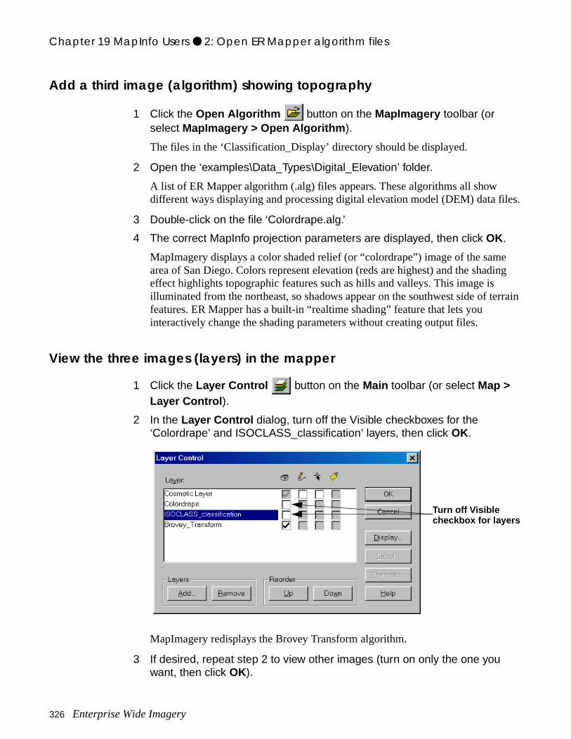
Chapter 19 MapInfo Users ● 2: Open ER Mapper algorithm files
iles.
e ing
errain
Add a third image (algorithm) showing topography
1 Click the Open Algorithm button on the MapImagery toolbar (or select MapImagery > Open Algorithm ).
The files in the ‘Classification_Display’ directory should be displayed.
2 Open the ‘examples\Data_Types\Digital_Elevation’ folder.
A list of ER Mapper algorithm (.alg) files appears. These algorithms all show different ways displaying and processing digital elevation model (DEM) data f
3 Double-click on the file ‘Colordrape.alg.’
4 The correct MapInfo projection parameters are displayed, then click OK.
MapImagery displays a color shaded relief (or “colordrape”) image of the samarea of San Diego. Colors represent elevation (reds are highest) and the shadeffect highlights topographic features such as hills and valleys. This image is illuminated from the northeast, so shadows appear on the southwest side of tfeatures. ER Mapper has a built-in “realtime shading” feature that lets you interactively change the shading parameters without creating output files.
View the three images (layers) in the mapper
1 Click the Layer Control button on the Main toolbar (or select Map > Layer Control ).
2 In the Layer Control dialog, turn off the Visible checkboxes for the ‘Colordrape’ and ISOCLASS_classification’ layers, then click OK.
MapImagery redisplays the Brovey Transform algorithm.
3 If desired, repeat step 2 to view other images (turn on only the one you want, then click OK).
Turn off Visiblecheckbox for layers
326 Enterprise Wide Imagery
Chapter 19 MapInfo Users ● 3: Overlay MapInfo vector data
the
-ocean
any
m an
4 If desired, save your workspace using File > Save Workspace .
5 Select File > Close All to close any open tables.
3: Overlay MapInfo vector data
Open an ER Mapper world topography algorithm
1 Click the Open Algorithm button on the MapImagery toolbar (or select MapImagery > Open Algorithm ).
2 Backup to the ‘examples’ folder, open the ‘applications’ folder, then open the ‘World_Topography’ folder.
A list of ER Mapper imagery (.ers) and algorithm (.alg) files appears.
3 Double-click on the ‘World_Topography.alg’ file.
4 If you see a message asking to overwrite the previous .tab file, click Yes.
5 Select the correct MapInfo projection items (as follows), then click OK:
• MapInfo Category–>Longitude / Latitude
• MapInfo Category Members–>Longitude / Latitude
• MapInfo Units –degrees
MapImagery displays a color shade relief image (a “colordrape”) of the world.Colors of the land areas represent elevation (magenta are the highest, red arelowest). Ocean areas are colored blue, and bathymetric features such as midridges are shown by the shading effect.
Note: When displaying data that is in a Longitude Latitude coordinate system, it is important to select ‘degrees’ as the map projection units. This lets you overlayother data that is also stored in degrees.
View Longitude Latitude coordinates on the image1 Select Map > Options .
2 On the Map Options dialog, select degrees for ‘Coordinate Units.’
Objectives Learn to overlay MapInfo vector and point table data on an ER Mapper algorithimage. In this case, you will display a world shaded relief image generated byER Mapper algorithm, then overlay MapInfo data of a Lat/Long grid, world capitals, and country borders.
Enterprise Wide Imagery 327
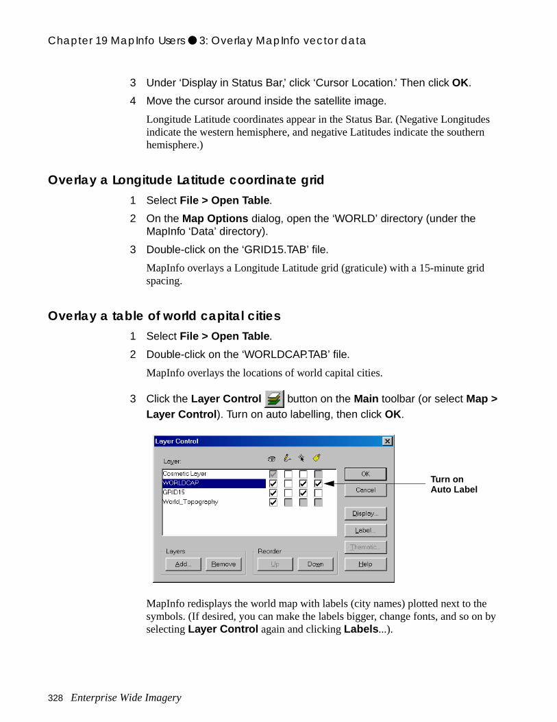
Chapter 19 MapInfo Users ● 3: Overlay MapInfo vector data
s n
by
3 Under ‘Display in Status Bar,’ click ‘Cursor Location.’ Then click OK.
4 Move the cursor around inside the satellite image.
Longitude Latitude coordinates appear in the Status Bar. (Negative Longitudeindicate the western hemisphere, and negative Latitudes indicate the southerhemisphere.)
Overlay a Longitude Latitude coordinate grid1 Select File > Open Table .
2 On the Map Options dialog, open the ‘WORLD’ directory (under the MapInfo ‘Data’ directory).
3 Double-click on the ‘GRID15.TAB’ file.
MapInfo overlays a Longitude Latitude grid (graticule) with a 15-minute grid spacing.
Overlay a table of world capital cities1 Select File > Open Table .
2 Double-click on the ‘WORLDCAP.TAB’ file.
MapInfo overlays the locations of world capital cities.
3 Click the Layer Control button on the Main toolbar (or select Map > Layer Control ). Turn on auto labelling, then click OK.
MapInfo redisplays the world map with labels (city names) plotted next to the symbols. (If desired, you can make the labels bigger, change fonts, and so onselecting Layer Control again and clicking Labels ...).
Turn onAuto Label
328 Enterprise Wide Imagery
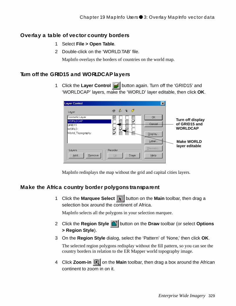
Chapter 19 MapInfo Users ● 3: Overlay MapInfo vector data
the
Overlay a table of vector country borders1 Select File > Open Table .
2 Double-click on the ‘WORLD.TAB’ file.
MapInfo overlays the borders of countries on the world map.
Turn off the GRID15 and WORLDCAP layers
1 Click the Layer Control button again. Turn off the ‘GRID15’ and ‘WORLDCAP’ layers, make the ‘WORLD’ layer editable, then click OK.
MapInfo redisplays the map without the grid and capital cities layers.
Make the Africa country border polygons transparent
1 Click the Marquee Select button on the Main toolbar, then drag a selection box around the continent of Africa.
MapInfo selects all the polygons in your selection marquee.
2 Click the Region Style button on the Draw toolbar (or select Options > Region Style ).
3 On the Region Style dialog, select the ‘Pattern’ of ‘None,’ then click OK.
The selected region polygons redisplay without the fill pattern, so you can seecountry borders in relation to the ER Mapper world topography image.
4 Click Zoom-in on the Main toolbar, then drag a box around the African continent to zoom in on it.
Turn off displayof GRID15 andWORLDCAP
Make WORLDlayer editable
Enterprise Wide Imagery 329
Chapter 19 MapInfo Users ● 4: MapImagery settings and options
ed
ts, e
the case
in le file. r all g,
how
Query the country data or go to other areas of the world1 If desired, use the MapInfo query tools to get information about the
countries, or follow the same steps as above to make country borders for other regions transparent.
2 (Optional.) Save your workspace using File > Save Workspace .
4: MapImagery settings and options
Table (.tab) files created by MapImageryWhen you open an ER Mapper imagery or algorithm file (or any other supportformat), MapImagery automatically creates a MapInfo table (.tab) file for the image. The table file contains information on the map projection, image extenviewing resolution, and other information MapInfo needs to properly display thimage. When you open an image or algorithm file that was already opened inpast, MapImagery prompts you to overwrite the previously created table file in you have changed any parameters since then.
You would want to overwrite the existing table file in the following cases:
• You selected the wrong map projection information the first time. Click Yes to overwrite the existing table file for the image, and select the correct projectioninformation for the future.
• You change the ‘Supersampling Factor’ on the MapImagery Options dialog’s Supersampling tab. This option lets you manipulate the quality of images withMapInfo, but is also tied to the image extents and coordinates saved in the tabIf you change the supersampling factor, you must regenerate the table files foimagery files you opened in the past. Click Yes to overwrite the existing table filefor the image to update the supersampling setting. (If you do not overwrite theexisting table file, your image will display but the map coordinates will be wronso this is very important.)
Algorithm (.alg) files created by MapImageryWhen you open an ER Mapper imagery (.ers) or other supported image file, MapImagery automatically creates an ER Mapper-format algorithm file for theimage (in addition to a MapInfo table file). The algorithm file tells MapImageryhow to display the image file, and is independent from the image file itself.
Objectives Learn to understand the way MapImagery handles and displays imagery, and to setup default options to control the way images are displayed and printed inMapInfo. (There are no exercises here, only information.)
330 Enterprise Wide Imagery
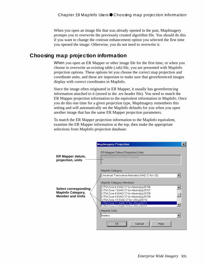
Chapter 19 MapInfo Users ● Choosing map projection information
ry this time
ou fo nd ages
e ce
When you open an image file that was already opened in the past, MapImageprompts you to overwrite the previously created algorithm file. You should do if you want to change the contrast enhancement option you selected the first you opened the image. Otherwise, you do not need to overwrite it.
Choosing map projection informationWhen you open an ER Mapper or other image file for the first time, or when ychoose to overwrite an existing table (.tab) file, you are presented with MapInprojection options. These options let you choose the correct map projection acoordinate units, and these are important to make sure that georeferenced imdisplay with correct coordinates in MapInfo.
Since the image often originated in ER Mapper, it usually has georeferencing information attached to it (stored in the .ers header file). You need to match thER Mapper projection information to the equivalent information in MapInfo. Onyou do this one time for a given projection type, MapImagery remembers this setting and will automatically set the MapInfo defaults for you when you openanother image that has the same ER Mapper projection parameters.
To match the ER Mapper projection information to the MapInfo equivalent, examine the ER Mapper information at the top, then make the appropriate selections from MapInfo projection database:
ER Mapper datum,projection, units
Select correspondingMapInfo Category,Member and Units
Enterprise Wide Imagery 331
Chapter 19 MapInfo Users ● The Supersampling setting
d
an
ints
led in
an
ic ay,
ption our
s” (or low e
If the
you rite
lues
The Supersampling settingWhen you open an ER Mapper or other image file, MapImagery processes andisplays the image data at a predefined resolution. This is called supersampling, and is controlled by the ‘Supersampling Factor’ on the MapImagery Options dialog’s Supersampling tab. For example, if you set supersampling to 8, then8x8 pixel area is displayed for every underlying pixel.
You should set the supersampling factor according to these guidelines:
• Use lower values to speed display of very large images, or mosaic algorithmscontaining many images. Lower values may not produce optimal hardcopy prhowever.
• Use higher settings to improve detail in on the screen when smoothing is enabthe ER Mapper algorithm, and when hardcopy printing from MapInfo.
Contrast enhancement optionsWhen you open an ER Mapper imagery (.ers) file and are prompted to createalgorithm for it, clicking Yes displays the Choose Algorithm Style dialog. This dialog lets you choose how contrast will be adjusted to improve the image presentation:
• Create an algorithm with No contrast stretching–This displays the image withoutenhancing the contrast. Use this option if you wish to view the image without enhancement or if your image is already contrast enhanced. Non-photographimages like digital terrain models (DEMs) may look better when displayed this wor may look better with contrast stretching.
• Create an algorithm with Automatic contrast stretching–This displays the imagewith a linear contrast enhancement to improve color and brightness. Use this ofor images that are not already contrast enhanced (like satellite images) or if yimages look too dark or light or lack contrast using the no stretching option.
The type of contrast enhancement applied is a linear contrast stretch that “clipsaturates) a certain percentage of brightest and darkest pixels at the high andends of the image histogram. The amount of clipping (percentage) is set in thMapImagery Options dialog’s Algorithm Generation tab. A 99% clip applies a mild contrast enhancement that look good on many types of images.image still lacks contrast, choose 97.5. (The smaller the percentage the morecontrast, but experiment for best results.)
Note: The algorithm file contains the contrast enhancement settings, so the setting choose is automatically applied to all images you open (if you choose to overwan existing algorithm file). If you have a problem image, try smaller percent vafor that image, then set the default back to 99% so it is used in the future.
332 Enterprise Wide Imagery
Chapter 19 MapInfo Users ● Contrast enhancement options
in
Close MapInfo
1 Close MapInfo by clicking the Close button on the application window or selecting File > Exit .
• Display an ER Mapper image file (.ers) as a MapInfo table file
• Display an ER Mapper algorithm file (.alg) as MapInfo table file
• Overlay MapInfo vector and tabular table data on an ER Mapper image
• Choose MapImagery setup options to control image display and printing
What you learned...
After completing these exercises, you know how to perform the following tasksMapInfo using the free MapImagery plug-in:
Enterprise Wide Imagery 333

Chapter 19 MapInfo Users ● Contrast enhancement options
334 Enterprise Wide Imagery

re to vers
n and
do ain orial.
ed to
odes, duse
20
Autodesk WorldUsers
This chapter explains how to use the capabilities of the Autodesk World softwadisplay ER Mapper imagery and algorithm files as backdrops. This chapter costeps similar to those described in the Autodesk World software documentatiohelp system.
Note: You must have a licensed copy of Autodesk World 2.0 to run this tutorial. You not need to have a copy of ER Mapper installed, but this is recommended to gaccess to sample ER Mapper imagery and algorithms used in the following tut(You can order the free ER Mapper installation CD-ROM from www.ermapper.com.)
About Autodesk World’s ER Mapper image viewing engineAs imagery data sources become more important for GIS applications, the neefficiently process, enhance and display large image files also becomes moreimportant. Many projects require the analysis of vector GIS drawing data by presenting it over image backdrops that show a “real world” perspective. For example, you gain a better understanding of parcel ownership, tax zones, zip cand many other vector entities by overlaying them on an airphoto showing lanand buildings.
Enterprise Wide Imagery 335
Chapter 20 Autodesk World Users ● Using Autodesk World with ER Mapper
rial y
are
age d s
re, ing
ms, eed
n tools
ies
Autodesk World incorporates the ER Mapper viewing engine, which lets you incorporate nearly any type of image data into your projects. These include aephotographs, satellite images, digital elevation (topography) images and manmore image types.
By incorporating the ER Mapper image viewing engine, Autodesk World usersnot restricted by limited image handling capabilities as are some other GIS products. You can directly display ER Mapper imagery and algorithms, and imformats with location information such as GeoTIFF, ESRI/GeoSPOT HDR, anothers. In addition, you can experience the full power of ER Mapper algorithmfrom within Autodesk World.
Using Autodesk World with ER MapperBy using Autodesk World in conjunction with a copy of the ER Mapper softwayou gain access to the extensive capabilities of this powerful integrated mappand image processing product, including:
• Import and display over 100 different image formats
• Use advanced image processing functions such as contrast enhancement, multispectral classification, vegetation indexes, color shaded reliefs, filtering, merging images, and many others.
• Directly read TIFF, GeoTIFF, Windows BMP, ER Mapper images and algorithESRI BIL, SPOTView and Universal Data Format (UDF) imagery without the nfor import or conversion
• Easily view the entire project area in one image–no limits on image file sizes
• Geocode, orthorectify or reproject imagery easily to precisely register with GISvector drawing data
• Automatically display, mosaic and color balance numerous images
• Combine imagery, vector and tabular data from any number of sources
• Create and edit vector data over imagery backdrops, and highlight features ofinterest and save them as vectors with ER Mapper’s raster to vector conversio
Hands-on exercisesThese exercises show you how to use the ER Mapper image display capabilitwithin Autodesk World.
• Insert an ER Mapper image into an Autodesk World drawing
What you will learn...
After completing these exercises, you will know how to perform the following tasks in Autodesk World:
336 Enterprise Wide Imagery
Chapter 20 Autodesk World Users ● 1: Inserting an ER Mapper image
t is, you e
ct.
r y or
.
• Enhance the image contrast and apply image smoothing
• Choose equivalent coordinate systems in Autodesk World and ER Mapper
• Insert an ER Mapper smart data algorithm into an Autodesk World drawing
• Stack and change the order of multiple images in a drawing
• Combine image and vector drawing data in a project
1: Inserting an ER Mapper image
The ER Mapper imagery (.ers) format stores image data in its “raw” form. Thathe imagery may not be processed or enhanced for best presentation. When insert an ER Mapper image, Autodesk World gives you options to enhance thimagery as it is loaded and displayed.
Start Autodesk World1 Start the Autodesk World software on your system.
2 Click the Maximize button in the upper-right corner of the Autodesk World application window (if it is not already maximized).
Autodesk World expands to fill your desktop. You should start with a new proje
3 If you do not already have a new (empty) project open, start one by choosing File > New , then clicking Blank Template .
4 If the Display Manager window is open, close it.
Before you begin...
Before beginning these exercises, you must have installed Autodesk World version 2.0 or higher on your system. These exercises use sample ER Mappeimagery and algorithm files from the ER Mapper installation CD-ROM. You maalso follow the general procedures using your own ER Mapper imagery (.ers) algorithm (.alg) files.
Objectives Learn to insert ER Mapper imagery (.ers) files into an Autodesk World drawing(You can also use the following procedure to open any image formats directlysupported by ER Mapper, including TIFF and GeoTIFF, Windows BMP, SPOTView, ESRI BIL, and others.)
Enterprise Wide Imagery 337
Chapter 20 Autodesk World Users ● 1: Inserting an ER Mapper image
n ld
ters of
sed by
F,
o,
Set the coordinate system for the new projectAll projects have an associated coordinate system. If you are beginning with aER Mapper image that has location information as your “basemap,” you shouchoose the same coordinate system as the image for your project.
1 Choose File > Properties .
2 Click the Coordinate System tab, then click Change....
3 On the Project Detail dialog, select UTM27-11 from the Coordinate System list.
This selection specifies a coordinate system using the NAD27 datum and theUniversal Transverse Mercator (UTM) map projection (zone 11 in the northernhemisphere). The coordinate units are meters, so locations are defined in meEastings and Northings.
4 Click OK on the Project Detail dialog, then click OK on the Project Properties dialog.
This coordinate system is now assigned to your project, and is the same one uthe ER Mapper images you will use in the upcoming examples.
Insert an ER Mapper-format (.ers) image into the drawing1 Choose Insert > ER Mapper Image .
2 On the Insert ER Mapper Image dialog, click the Image tab, then click Browse .
3 Double-click on the folder where ER Mapper is installed, then open the ‘examples/Applications/Airphoto/1_Geocoding’ folder.
A list of ER Mapper algorithm (.alg) files appears.
4 Turn off the ‘Bilinear Smoothing’ and ‘Contrast Stretching’ options. (These will be explained later).
5 Click on the ‘Files of Type’ list to view the different image formats.
You can insert ER Mapper algorithms (.alg) and datasets (.ers), as well as TIFBMP, ARC/INFO-GeoSPOT HDR, and others.
6 From the ‘Files of Type’ list, select Datasets (*.ers) .
7 Double-click on the file ‘San_Diego_Airphoto_34_rectified.ers.’
8 Click the Zoom All button or choose View > Zoom All .
Autodesk World displays a color aerial photograph of the downtown San DiegCalifornia area. This image has been rectified to the NAD27 datum and UTM zone11 map projection, so it has geographic location information (true earth coordinates).
338 Enterprise Wide Imagery
Chapter 20 Autodesk World Users ● 1: Inserting an ER Mapper image
e the
ge,
usly you
nded dark
Zoom in to a small area to see the pixel resolution
1 Click the Zoom Window button (or choose View > Zoom Window ), then drag a very small box over part of the photo to zoom into it.
If needed, do this again until you can see the small square areas that comprisdigital image. These squares are called pixels (for picture elements), and are roughly equivalent to the smallest object you can see in the photo. In this imaeach pixel is about 1 meter in diameter, which is termed “1-meter resolution.”
Reload the image with smoothing and contrast enhancement1 Choose Insert > ER Mapper Image .
2 This time turn on the ‘Bilinear Smoothing’ and ‘Contrast Stretching’ options.
3 From the ‘Files of Type’ list, select Datasets (*.ers) .
4 Click Browse , then double-click on the file ‘San_Diego_Airphoto_34_rectified.ers’ again to reload it.
The airphoto image redisplays with improved contrast and a “smoother” appearance.
• Bilinear Smoothing improves the display of zoomed images or large hardcopyprints by averaging the pixel values to remove the “blocky” look you saw previowhen smoothing was not turned on. (You only see the effect of smoothing whenzoom into the pixel level.)
• Contrast Stretching generally improves the image color and presentation by increasing contrast between the light and dark areas. This option is recommewhen inserting most image files, otherwise they may lack contrast or look too or light.
Zoom in and out in the image
1 Click the Zoom All button or choose View > Zoom All .
The image zooms out to display the full extents of the airphoto.
2 Click the Zoom Window button (or choose View > Zoom Window ), then drag a box over the central part of the photo to zoom into it.
3 Click the Zoom In or Zoom Out buttons, then click on the image to zoom in or out by fixed amounts.
4 When finished, click the Zoom All button or choose View > Zoom All to zoom out to the full image extents.
Enterprise Wide Imagery 339
Chapter 20 Autodesk World Users ● 1: Inserting an ER Mapper image
e he
5 Once again, click Zoom Window , then drag a box over the central part of the photo to zoom into it.
Pan (scroll) the image
1 Click the Pan 2 Points button (or choose View > Pan ). Click on one point in the photo, then click on a second point.
The image pans (scrolls) in the direction and distance you defined by your twopoints. This is one way to view adjacent areas of an image.
2 Drag the scroll bars on the right or lower areas of the project window.
The image pans in the direction you drag the scroll bar.
View geographic coordinates on the image1 Choose Tools > Format Options .
2 Click the Coordinate tab, select Latitude Longitude from the ‘Display Type’ list, then click OK.
3 Point to various locations in the image.
The Latitude Longitude coordinates of the current cursor location appear in thstatus bar. (The format is decimal degrees, and negative longitudes indicate twestern hemisphere.)
4 Choose Tools > Format Options again.
5 Click the Units tab, then select m from the ‘User Unit’ list.
6 Click the Coordinate tab, select Projection Coordinate from the ‘Display Type’ list, then click OK.
7 Point to various locations in the image.
The UTM map projection coordinates appear in the status bar. (The format is meters of Northings and Eastings in UTM zone 11.)
Close the project1 Choose File > Close .
When asked to save the contents or save changes, click No.
340 Enterprise Wide Imagery
Chapter 20 Autodesk World Users ● 2: Inserting multiple coregistered images
r n or
you
ust
of
2: Inserting multiple coregistered images
An ER Mapper algorithm is a list of processing steps or instructions ER Mappeuses to transform a raw image file into a final, enhanced image on your screeprinter. An algorithm does not contain the actual image data, but only stores references to it. (The actual image data is stored in ERS or other files.) Wheninsert an ER Mapper algorithm into an Autodesk World drawing, it follows the steps in the algorithm and displays the finished image accordingly.
Note: In order to precisely overlay multiple images (as you will do next), the images mhave the same coordinate system information.
Start a new project1 Start a new project by choosing File > New , then clicking Blank Template .
Set the coordinate system for the new project1 Choose File > Properties .
2 Click the Coordinate System tab, then click Change....
3 On the Project Detail dialog, select UTM27-11 from the Coordinate System list.
Set the data viewing coordinate type1 Choose Tools > Format Options .
2 Click the Units tab, then select m from the ‘User Unit’ list.
3 Click the Coordinate tab, select Projection Coordinate from the ‘Display Type’ list, then click OK.
The display coordinates are now set to the units of the map projection (metersNorthings and Eastings in UTM zone 11.)
Objectives Learn to insert ER Mapper smart data algorithm (.alg) files into an Autodesk World drawing. Also learn to “stack” multiple images covering the same geographic area, and to turn images on/off and move them to the top of the display.
Enterprise Wide Imagery 341
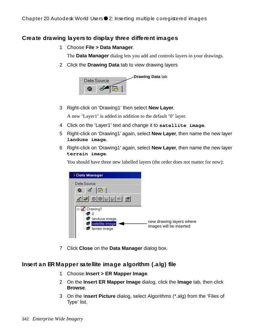
Chapter 20 Autodesk World Users ● 2: Inserting multiple coregistered images
:
Create drawing layers to display three different images1 Choose File > Data Manager .
The Data Manager dialog lets you add and controls layers in your drawings.
2 Click the Drawing Data tab to view drawing layers
3 Right-click on ‘Drawing1’ then select New Layer .
A new ‘Layer1’ is added in addition to the default ‘0’ layer.
4 Click on the ‘Layer1’ text and change it to satellite image .
5 Right-click on ‘Drawing1’ again, select New Layer , then name the new layer landuse image .
6 Right-click on ‘Drawing1’ again, select New Layer , then name the new layer terrain image .
You should have three new labelled layers (the order does not matter for now)
7 Click Close on the Data Manager dialog box.
Insert an ER Mapper satellite image algorithm (.alg) file1 Choose Insert > ER Mapper Image .
2 On the Insert ER Mapper Image dialog, click the Image tab, then click Browse .
3 On the Insert Picture dialog, select Algorithms (*.alg) from the ‘Files of Type’ list.
Drawing Data tab
new drawing layers whereimages will be inserted
342 Enterprise Wide Imagery
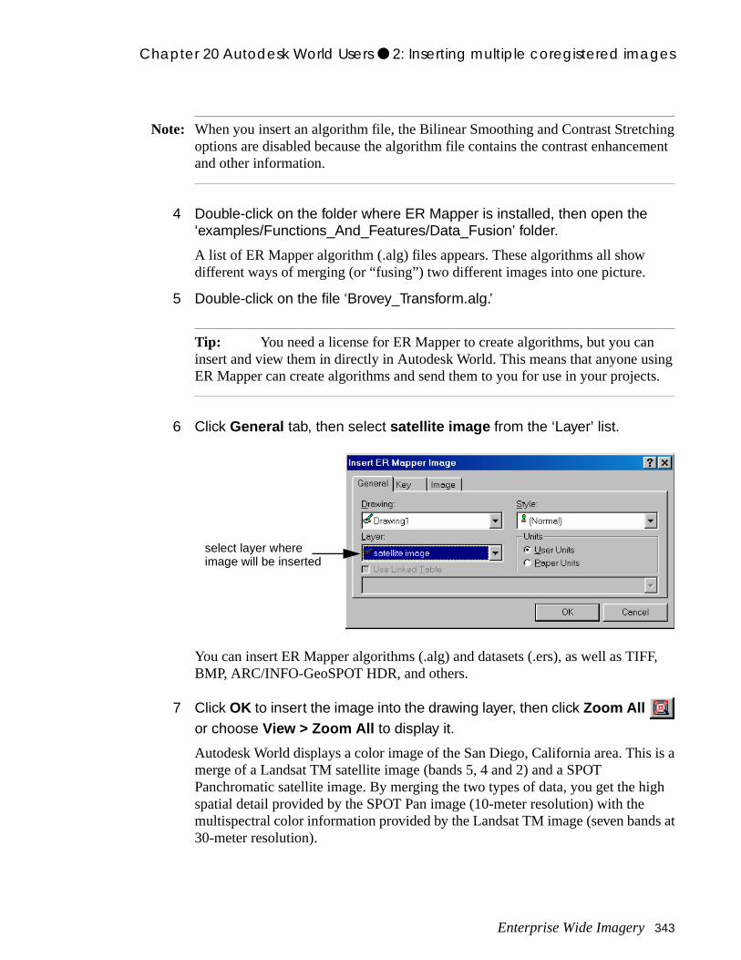
Chapter 20 Autodesk World Users ● 2: Inserting multiple coregistered images
hing ment
sing ts.
F,
is a
igh
s at
Note: When you insert an algorithm file, the Bilinear Smoothing and Contrast Stretcoptions are disabled because the algorithm file contains the contrast enhanceand other information.
4 Double-click on the folder where ER Mapper is installed, then open the ‘examples/Functions_And_Features/Data_Fusion’ folder.
A list of ER Mapper algorithm (.alg) files appears. These algorithms all show different ways of merging (or “fusing”) two different images into one picture.
5 Double-click on the file ‘Brovey_Transform.alg.’
Tip: You need a license for ER Mapper to create algorithms, but you caninsert and view them in directly in Autodesk World. This means that anyone uER Mapper can create algorithms and send them to you for use in your projec
6 Click General tab, then select satellite image from the ‘Layer’ list.
You can insert ER Mapper algorithms (.alg) and datasets (.ers), as well as TIFBMP, ARC/INFO-GeoSPOT HDR, and others.
7 Click OK to insert the image into the drawing layer, then click Zoom All
or choose View > Zoom All to display it.
Autodesk World displays a color image of the San Diego, California area. Thismerge of a Landsat TM satellite image (bands 5, 4 and 2) and a SPOT Panchromatic satellite image. By merging the two types of data, you get the hspatial detail provided by the SPOT Pan image (10-meter resolution) with the multispectral color information provided by the Landsat TM image (seven band30-meter resolution).
select layer whereimage will be inserted
Enterprise Wide Imagery 343
Chapter 20 Autodesk World Users ● 2: Inserting multiple coregistered images
at d to
-date
me
o. e
ith se or
The Brovey Transform is a mathematical way of combining the two images thalso greatly enhances the color. Merging or fusion techniques like this are usecreate to combine the strengths of different satellite sensors and create up-toviews of the earth’s surface.
8 Click Zoom Window (or choose View > Zoom Window ), then drag a box over the central part of the image to zoom into it.
The image shows a high resolution, color-enhanced view of the area. The ER Mapper algorithm creates this image interactively from the two separate Landsat and SPOT satellite imagery files. (The Brovey Transform technique usually requires up to three intermediate image files to be created when usingtraditional imaging software, but ER Mapper performs the processing in real tifrom the two source images without creating intermediate files.)
9 When finished, click the Zoom All button or choose View > Zoom All to zoom out to the full image extents.
Insert a second algorithm image showing thematic landuse1 Choose Insert > ER Mapper Image .
2 On the Insert ER Mapper Image dialog, click the Image tab, then click Browse .
3 Double-click on the folder where ER Mapper is installed, then open the ‘examples/Functions_And_Features/Classification_Display’ folder.
A list of ER Mapper algorithm (.alg) files appears. These algorithms all show different ways of merging (or “fusing”) two different images into one picture.
4 Double-click on the file ‘Isoclass_classification.alg.’
5 Click General tab, then select landuse image from the ‘Layer’ list.
6 Click OK to insert the image into the layer and display it.
Autodesk World displays a thematic color image of the same area of San DiegDifferent colors correspond to different types of landuse in the area. This imagwas created from a 1985 Landsat TM satellite image using ER Mapper’s ISOCLASS unsupervised classification feature. Classification groups pixels wsimilar spectral values into classes that can represent different types of landuland cover.
Insert a third algorithm image showing terrain and topography1 Choose Insert > ER Mapper Image .
2 On the Insert ER Mapper Image dialog, click the Image tab, then click Browse .
344 Enterprise Wide Imagery
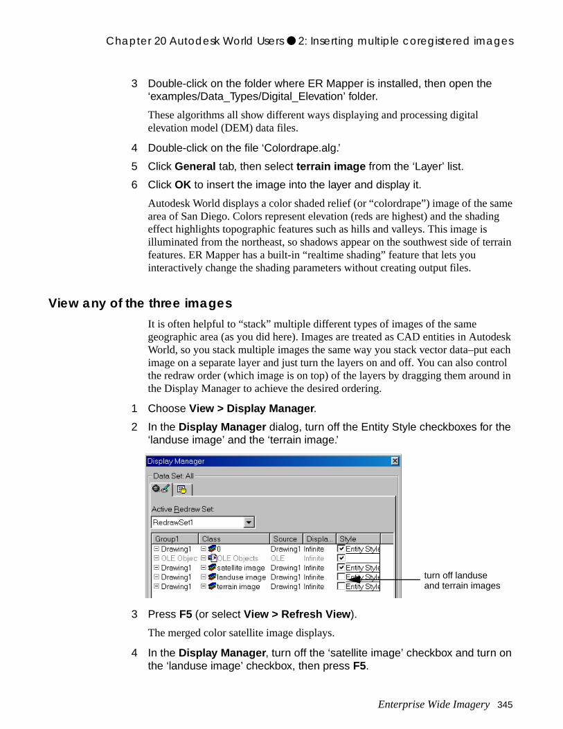
Chapter 20 Autodesk World Users ● 2: Inserting multiple coregistered images
ame ing
errain
desk each ntrol d in
3 Double-click on the folder where ER Mapper is installed, then open the ‘examples/Data_Types/Digital_Elevation’ folder.
These algorithms all show different ways displaying and processing digital elevation model (DEM) data files.
4 Double-click on the file ‘Colordrape.alg.’
5 Click General tab, then select terrain image from the ‘Layer’ list.
6 Click OK to insert the image into the layer and display it.
Autodesk World displays a color shaded relief (or “colordrape”) image of the sarea of San Diego. Colors represent elevation (reds are highest) and the shadeffect highlights topographic features such as hills and valleys. This image is illuminated from the northeast, so shadows appear on the southwest side of tfeatures. ER Mapper has a built-in “realtime shading” feature that lets you interactively change the shading parameters without creating output files.
View any of the three imagesIt is often helpful to “stack” multiple different types of images of the same geographic area (as you did here). Images are treated as CAD entities in AutoWorld, so you stack multiple images the same way you stack vector data–put image on a separate layer and just turn the layers on and off. You can also cothe redraw order (which image is on top) of the layers by dragging them arounthe Display Manager to achieve the desired ordering.
1 Choose View > Display Manager .
2 In the Display Manager dialog, turn off the Entity Style checkboxes for the ‘landuse image’ and the ‘terrain image.’
3 Press F5 (or select View > Refresh View ).
The merged color satellite image displays.
4 In the Display Manager , turn off the ‘satellite image’ checkbox and turn on the ‘landuse image’ checkbox, then press F5.
turn off landuseand terrain images
Enterprise Wide Imagery 345
Chapter 20 Autodesk World Users ● 3: Combining image and drawing data
ithms ur
to if
ge.
5 View any of the three images by turning on its layer and turning the other two off, then pressing F5 to refresh the view.
These simple examples show how you can use the power of ER Mapper algorto showing various “views” of your image data as backdrops for analysis of yovector data in Autodesk World.
Close the project1 If desired, save your project using File > Save As... .
2 Choose File > Close to close the project.
3: Combining image and drawing data
Note: Before beginning, make sure the ‘AutoCAD DXF’ GDX driver has been addedAutodesk World. Consult your Autodesk World documentation or on-line help needed to do this before continuing.
Start a new project1 Start a new project by choosing File > New , then clicking Blank Template .
Set the coordinate system for the new project1 Choose File > Properties .
2 Click the Coordinate System tab, then click Change....
3 On the Project Detail dialog, select UTM27-11 from the Coordinate System list.
Set the data viewing coordinate type1 Choose Tools > Format Options .
2 Click the Units tab, then select m from the ‘User Unit’ list.
3 Click the Coordinate tab, select Projection Coordinate from the ‘Display Type’ list, then click OK.
Objectives Learn to use both image (raster) and drawing (vector) data in a project. In thisexample, you will overlay a network of roads on a small aerial photograph ima
346 Enterprise Wide Imagery
Chapter 20 Autodesk World Users ● 3: Combining image and drawing data
of
wn
The display coordinates are now set to the units of the map projection (metersNorthings and Eastings in UTM zone 11.)
Create a drawing layer to display an airphoto image1 Choose File > Data Manager .
2 Click the Drawing Data tab to view drawing layers.
3 Right-click on ‘Drawing1’ then select New Layer .
4 Click on the ‘Layer1’ text and change it to airphoto image .
Insert an ER Mapper airphoto image into the drawing1 Choose Insert > ER Mapper Image .
2 On the Insert ER Mapper Image dialog, click the Image tab, then click Browse .
3 From the ‘Files of Type’ list, select Datasets (*.ers) .
4 Double-click on the folder where ER Mapper is installed, then open the ‘examples/Shared_Data’ folder.
5 Double-click on the file ‘Airphoto.ers.’
6 Turn on the ‘Bilinear Smoothing’ and ‘Contrast Stretching’ options.
7 Click General tab, then select airphoto image from the ‘Layer’ list.
8 Click OK to insert the image into the layer and display it.
9 Click the Zoom All button or choose View > Zoom All .
Autodesk World displays a color aerial photograph of small part of the downtoSan Diego, California area.
Open a DXF drawing to overlay on the airphoto image1 Choose File > Data Manager .
2 Click the Drawing Data tab, then click the Open Drawing button.
3 From the ‘Files of Type’ list, select Autodesk DXF File (*.dxf) .
Note: If ‘Autodesk DXF’ does not appear as a filetype option, you need to install theAutoCAD DXF GDX driver.
4 Open the ER Mapper ‘examples/Data_Types_AutoCAD_DXF’ folder.
Enterprise Wide Imagery 347
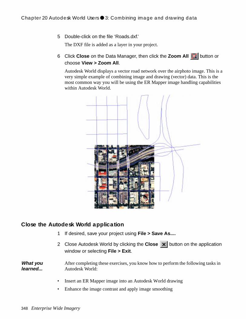
Chapter 20 Autodesk World Users ● 3: Combining image and drawing data
is a e es
in
5 Double-click on the file ‘Roads.dxf.’
The DXF file is added as a layer in your project.
6 Click Close on the Data Manager, then click the Zoom All button or choose View > Zoom All .
Autodesk World displays a vector road network over the airphoto image. This very simple example of combining image and drawing (vector) data. This is thmost common way you will be using the ER Mapper image handling capabilitiwithin Autodesk World.
Close the Autodesk World application1 If desired, save your project using File > Save As....
2 Close Autodesk World by clicking the Close button on the application window or selecting File > Exit .
• Insert an ER Mapper image into an Autodesk World drawing
• Enhance the image contrast and apply image smoothing
What you learned...
After completing these exercises, you know how to perform the following tasksAutodesk World:
348 Enterprise Wide Imagery

Chapter 20 Autodesk World Users ● 3: Combining image and drawing data
• Choose equivalent coordinate systems in Autodesk World and ER Mapper
• Insert an ER Mapper smart data algorithm into an Autodesk World drawing
• Stack and change the order of multiple images in a drawing
• Combine image and vector drawing data in a project
Enterprise Wide Imagery 349

Chapter 20 Autodesk World Users ● 3: Combining image and drawing data
350 Enterprise Wide Imagery
hat ds-on ages
pace be
A
System setupThis appendix describes the steps needed to install the training datasets so tstudents can perform the hands-on exercises in this manual. Most of the hanexercises in this workbook require students to access the airphoto example imsupplied with ER Mapper 6.
Note: Before beginning the installation, you must have at least 450 Mb of free disk s(310 Mb for the files on the CD-ROM and 140 Mb additional space for files tocreated during the exercises.)
Windows installation of training datasets1 Create a new directory named “airphoto_training” inside the directory
ERMAPPER/dataset.
This is the directory where the training datasets are assumed to reside.
2 Use the Windows File Manager or Explorer to copy all the files on the CD-ROM into the “ERMAPPER/dataset/airphoto_training” directory.
The datasets are now accessible to users performing the exercises.
The datasets are now accessible to users performing the exercises.
ER Mapper Workbook - Airphoto Mosaic Applications 351

Appendix A#System setup z Windows installation of training datasets
352 ER Mapper Workbook - Airphoto Mosaic Applications
tion nt to
B
Reference textsThis appendix provides references to textbooks that describe uses, interpretaand processing of airphotos. These books will be very helpful to those who walearn more about interpretation of airphotos and their applications, and also contain many references to other sources of data and publications.
Avery, E. A., and G. L. Berlin. 1992. Fundamentals of Remote Sensing and Airphoto Interpretation, Macmillan Publishing Company, New York, N.Y, USA.
Faulkner, E. 1995. Aerial Mapping: Methods and Applications, CRC Press, Boca Raton, Fla. USA.
Lillesand, T. M., and R. W. Kiefer. 1991. Remote Sensing and Image Interpretation, John Wiley and Sons, Inc. New York, N.Y, USA.
ER Mapper Workbook - Airphoto Mosaic Applications 353

Appendix # z
354 ER Mapper Workbook - Airphoto Mosaic Applications
IndexAairphotos
annotating 227color balancing 157composing maps 217contrast enhancement 59exporting 245haze (blue cast) removal 172importing 54mosaic creation 20, 141rectifying (geocoding) 89saving and exporting 253scanning 19scanning and display 74types 18viewing overlap areas 181
Algorithm dialogoverview 51
Algorithm Geoposition Extents dialog boxExtents options 204Geolink options 263Zoom options 43
algorithm layers. See layersalgorithms
basic concepts 28, 49, 74changing color table 58commenting 69
ER Mapper Workbook - Airphoto Applications 355
Index
creating automatically 50creating manually 50entering description 69, 87mosaics 143, 160, 166, 208opening 38plotting as map object 241printing 242process diagram 52saving 69, 87, 155, 170, 194, 199, 201, 205, 214using as templates 51
annotation. See map compositionArcView GIS 301
ER Mapper imagery extension 301ArcView GIS ER Mapper plug-in
how to obtain 302loading 303opening ER Mapper images 304overview 301tutorial 303using with ER Mapper 302vector data 310zoom and pan 306, 315
autoclip transformconcept 65setting percent clip 203
Autodesk productssave/export from ER Mapper 255
Autodesk World 335bilinear smoothing 339contrast enhancement 339inserting ER Mapper images 337setting coordinate system 338tutorial 335using images and drawing data 346using multiple images 341
Ccamera calibration report 113Camera file 122Camera Wizard 117
Camera attributes page 119Camera identification page 118Fiducial point offsets page 121Focal length 119
356 ER Mapper Workbook - Airphoto Applications
Index
Number of Fiducial points page 120X offset to principal point 119Y offset to principal point 119
clip masks for maps 224Color (RGB) 247Color Balancing Wizard for Airphotos 209Color Mode
relation to layer type 86color tables 58comments
defining 69viewing 71
composing maps. See map compositioncompression of imagery 280Compression Wizard
Actual compression ratio 249Compress to Grayscale or RGB 247saving the compressed image 247Target Compression ratio 248
contrast enhancement 59automatic 67manual 62
Ddata structure diagram 51dialog boxes 32
text entry 34displaying datasets 57
EEnterprise wide imagery 277
definition 278free ER Mapper plug-ins 279problems 277solutions 279
ER Mappercompression technology 280dialog boxes 32file choosers 33help system 34introduction 17, 317main menu 31product capabilities 279
ER Mapper Workbook - Airphoto Applications 357
Index
raster datasets 22toolbars 31user interface 29vector datasets 22
ER Mapper plug-insfor ArcView GIS 301for MapInfo (MapImagery) 317for office applications 291
ER Viewer 283how to obtain 283measuring distances 287opening images 285panning (roaming) images 287printing images 289product capabilities 283tutorial 284using as OLE server 291viewing image properties 289zooming (magnifying) images 286
ESRI ArcView GIS 301ESRI products
save/export from ER Mapper 255exporting data 25, 253
resampling cell size 261, 264, 269to Autodesk products 255to ESRI .hdr format 264to MapInfo 255to TIFF format 266
Ffeathering images 180, 192fiducial points 123file chooser dialog boxes 33free imagery plugins for GIS and office applications 245
GGaussian equalization 66
setting std. dev. 67GCP Edit dialog box 130GCP Setup tab 126Geocode Output Extents dialog 132geocoding
advanced orthorectification 113
358 ER Mapper Workbook - Airphoto Applications
Index
camera calibration report 113Compute FROM function 101GCP display options 103picking first 4 GCPs 97picking points from overview 101RMS errors 100
Geocoding Wizard 113Auto zoom 129Auto Zoom option 103Calculate from point button 101Cell Attributes box 107Exterior Orientation Setup tab 135Fiducial Point Edit tab 122, 135GCP Edit tab 98, 103, 127GCP Setup tab 126Ortho Setup tab 116, 135Orthorectify using exterior orientation 116, 134Output Coordinate Space dialog 127Rectify tab 106, 131, 137resampling 107Use a DEM file as height 117Zoom to current GCP button 103
geocoding. See rectificationGID Australia 317GIS systems
exporting images to 245raster image formats 255resampling cell size for 254subsetting images for 254using images in 253
graphics formatsexporting to 25using in map composition 241
ground control pointsadjusting 103labelling 105locking 105overview 90picking 98saving to dataset 106viewing error bars 103
Hhardcopy printing 25
ER Mapper Workbook - Airphoto Applications 359
Index
haze corrections 172help system 34histogram equalization 66
IImage Display and Mosaic Wizard 76, 160Image Display and Mosaicing Wizard 149image files. See raster datasetsimage processing
concepts 25enhancements 23ER Mapper algorithms 27traditional techniques 27
image rectification parameters 127image windows
closing 46loading datasets 57measuring distances 111moving 39moving to front 45opening 38panning with buttons 42resizing 40selecting current 46shaping to fit image 152using multiple windows 44viewing coordinates 110zooming with buttons 42zooming with mouse 41
imagerycompression 281file formats 277file sizes 277, 281served over the internet 278, 279sharing among applications 277sharing via OLE 291using in office applications 291
importing airphoto images 55
LLayer tab 52layers 52
adding 83
360 ER Mapper Workbook - Airphoto Applications
Index
Annotation/Map Composition 217changing type 84deleting 83dragging and dropping 147duplicating 84labelling 68loading data into 82moving between 85, 203, 204moving up or down 81selecting 79selecting bands 84setting display priority 147shortcut menu 84, 147with Color Mode 86
Line Style dialog box 228loading datasets 57
OK vs Apply button 82
Mmagnifying images. See zoomingmap composition
adding inset images 241area of polygon 229basic concepts 217clip masks 224deleting objects 230drag and drop objects 237drawing annotation 228drawing map objects 234duplicating (cloning) objects 231Fast Preview option 238importing graphics formats 241importing text 241length of line 228object attributes 241object selection tools 230page background color 223Page Relative option 241Page Setup options 242polygon attributes 229polyline attributes 228resizing/positioning objects 239saving to disk 239selecting multiple objects 231
ER Mapper Workbook - Airphoto Applications 361
Index
selecting objects 228setting map object attributes 225, 236special features 241text attributes 231, 232
map projections. See rectification 113MapImagery plug-in 317
algorithm (.alg) files created by 330commercial version 318contrast enhancement 332controlling image layers 326free version 317how to obtain 318measuring distances 321opening ER Mapper algorithms 322opening ER Mapper images 320overlaying vector data 327setting image map projection 321, 331table (.tab) files created by 330tutorial 318using with ER Mapper 318viewing image coordinates 322zoom and pan 321
MapInfo 317export from ER Mapper 255link with ER Mapper 255MapImagery plug-in 317
measuring distances 111mensuration 111Microsoft Office applications 291mosaicing 20
analyze images 209basic steps 21capabilities 142creating algorithms 143, 208display band 151display method 151feathering 210file types 150mosaic properties 150requirements 141RGB 123 154setting display priority 142, 147turning images on/off 147, 153zooming to all datasets 146
mosaickingcreating algorithms 160, 166
362 ER Mapper Workbook - Airphoto Applications
Index
viewing overlap areas 181zooming to all datasets 164
mouse buttons 30mouse pointer
Hand mode 41Pointer mode 110shapes 30Zoom mode 40ZoomBox mode 41
OObject Linking and Embedding (OLE) 291office applications
using imagery in 291OLE
displaying images 294drag and drop images 295overview 292tutorial 291
orthorectificationAttitude kappa 114, 136Attitude omega 113, 136Attitude phi 114, 136Camera Wizard 117Exposure center X Y Z 136exterior orientation 114, 116, 135, 136fiducial points 124Focal length 119Scale 137X offset to principal point 119Y offset to principal point 119
PPage Setup dialog box 220panning images
with buttons 43with mouse 41
polygon attributes 229area measurement 229color and shading 229
polyline attributes 228, 229polylines
color and style attributes 228
ER Mapper Workbook - Airphoto Applications 363
Index
editing points 228length (geographic units) 228smoothing (spline) 228
Postscript filesprinting to 25using in map composition 217
printing images 25, 242process stream diagram 52Pseudocolor color mode 58
RRaster Dataset dialog 82
Apply button 82OK vs Apply buttons 82
raster datasetsdescription 26importing 22mosaicing 177, 195, 207mosaics 141opening directly 75
raster imagesmosaicing 207
rectification 23adjusting GCPs 103Compute FROM function 101GCP display options 103, 130picking first 4 GCPs 97picking points from overview 101RMS errors 100
Red Green Blue (RGB) color mode 73Refresh Image button 39regions 177
defining 183hidden stitch lines 178naming 185, 187referencing in formulas 189
RMS errors 100
Ssaving data 253
cropping/subsetting 254for Autodesk products 255for MapInfo 255
364 ER Mapper Workbook - Airphoto Applications
Index
in UDF format 257resampling cell size 261, 264, 269to ESRI .hdr format 264to TIFF format 266
shortcut menuslayers 147surfaces 181
surfaces 52changing color mode 181expanding/contracting 80shortcut menu 181
Ttab pages 52text attributes 231Text Style dialog box 231toolbars
displaying 37hiding 37overview 31using 37
Transform dialog box 60transforms
autoclipping 65, 203Gaussian equalization 66histogram equalization 66viewing 60viewing for other layers 85, 203, 204
UUDF images 257
VView Mode 52vignetting 158
Wwarping images. See rectification 113wavelet compression technology 245
ER Mapper Workbook - Airphoto Applications 365
Index
wavelet image compression 280windows. See image windowsword processing
inserting images via OLE 291
Zzooming images
out to full extents 42, 44to current dataset extents 148to page extents or contents 227to specific dataset extents 153with buttons 43with mouse 41
366 ER Mapper Workbook - Airphoto Applications