EMPIRICAL EVIDENCE ON THE EFFECTS OF STABILIZATION POLICY

Laurence H. Meyer and Robert H. Rasche

Macroeconometric research in the 1970s has been dominated by the

refinement of large-scale income-expenditure macroeconometric models,

the attenpt to reconcile the policy multipliers derived from these

models with those yielded by simple reduced-forms, the refinement and

estimation of the relation between inflation and unemployment, and the

application of optimal control techniques to macroeconometric models.

These four themes provide the focus for this paper.

The first section reviews the implications of various nacroeco-

nonetric models for monetary and fiscal multipliers. We are particu-

larly concerned here with the degree of consensus across models and the

evolution of estimated models over time. The second section discusses

attempts to reconcile the divergent implications of income-expenditure

structural nodels and the St. Louis reduced-form for fiscal policy

multipliers. In the third section we develop the implications of esti-

mated Phillips curve equations and monetarist models for the response

of unemployment, output, and inflation to traditional demand management

policies. And in the fourth section we consider the accumulated evi-

dence on the gains from policy activism, drawing on the results of

optimal control sinulations with a variety of nacroeconometric models.

Laurence H. Meyer is Associate Professor of Economics at WashingtonUniversity and Visiting Scholar at the Federal Reserve Bank of St.Louis. Robert H. Rasche is Professor of Economics at Michigan StateUniversity.

-41-

During the last half of the ‘70s increased attention has been

focused on the way in which economic agents form expectations, particu-

larly inflation expectations, and on “equilibrium” macroeconomic models

embodying “rational expectations.” These models yield dramatic con-

clusions about both the costs of eradicating inflation and the gains

from activism. We therefore consider the implications of rational ex-

pectation models in both the third and fourth sections, although there

is as yet only a small literature on empirical applications of these

models to draw upon.

A COMPARISON OF POLICY MULTIPLIERS ACROSS MODELS AND TIME

In this section we review the evidence from structural models and

reduced-forms about the size and time pattern of policy multipliers.

We are interested in the average size of multipliers, the consensus

across models, and the evolution over time in the estimated multipliers.

A Comparison of Multipliers_Across_Models

Christ (1975) has surrgnarized the consensus across models rather

pessimistically: “. . . though models forecast reasonably well over

horizons of four to six quarters, they disagree so strongly about the

effects of important monetary and fiscal policies that they cannot be

considered reliable guides to such policy effects, until it can be de-

termined which of them are wrong in this respect and which (if any) are

right.” (p. 54)

Tables 1, 2, and 3 present policy multipliers from seven econo-

metric models (Bureau of Economic Analysis (BEA), Brookings (B), Univer-

sity of Michigan (MQEM), Data Resources, Inc. (DRI), Federal Reserve

Bank of St. Louis (St.L), MIT-Pennsylvania—SSRC (MPS), and Wharton (W))

—42—

as reported in Fronin and Klein (1976). The multipliers are reported

for the first quarter and fourth, eighth, twelfth, sixteenth, and

twentieth quarters and for three policy changes —— an increase in real

government expenditures on goods and services, a decline in personal

taxes, and an increase in either the money supply or nonborrowed re-

serves. The mean and coefficients of variation for the various multi-

pliers are also reported.1

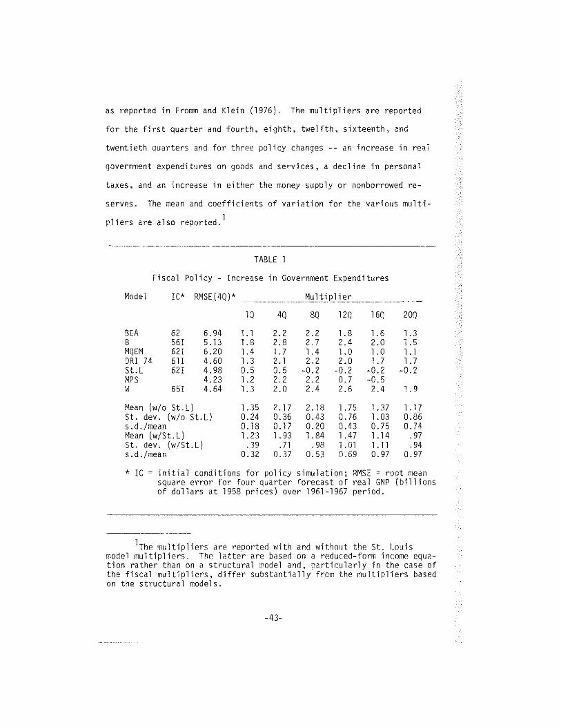
TABLE 1

Fiscal Policy - Increase in Government Expenditures

Model IC* RMSE(4Q)* Multiplier

lQ 4Q SQ l2Q l6Q 20Q

BEA 62 6.94 1.1 2.2 2.2 1.8 1.6 1.3B 561 5.13 1.8 2.8 2.7 2.4 2.0 1.5MQEM 621 6.20 1.4 1.7 1.4 1.0 1.0 1.1DRI 74 611 4.60 1.3 2.1 2.2 2.0 1.7 1.7St.L 621 4.98 0.5 0.5 —0.2 —0.2 -0.2 —0.2MPS 4.23 1.2 2.2 2.2 0.7 -0.5W 651 4.64 1.3 2.0 2.4 2.6 2.4 1.9

Mean (w/o 5t.L) 1.35 2.17 2.18 1.75 1.37 1.17St. dev. (w/o St.L) 0.24 0.36 0.43 0.76 1.03 0.86s.d./mean 0.18 0.17 0.20 0.43 0.75 0.74Mean (w/St.L) 1.23 1.93 1.84 1.47 1.14 .97St. dev. (w/St.L) .39 .71 .98 1.01 1.11 .94s.d./mean 0,32 0.37 0.53 0.69 0.97 0.97

* IC = initial conditions for policy simulation; RMSE = root meansquare error for four quarter forecast of real GNP (billionsof dollars at 1958 prices) over 1961-1967 period.

1The multipliers are reported with and without the St. Louismodel multipliers. The latter are based on a reduced-form income equa-tion rather than on a structural model and, particularly in the case ofthe fiscal multipliers, differ substantially from the multipliers basedon the structural models.

—43—

The mean fiscal expenditure multiplier is just over 1—1/4 in the

first quarter and builds to 2—1/4 by the end of year two; however, the

cumulative multiplier is still over one after five years. While there

is considerable consensus about the multipliers through the first three

years, the agreement deteriorates sharply. Note that in all cases the

multiplier peaks within three years, generally within four to eight

quarters; and cumulative fiscal multipliers fall to zero or below by

the fifth quarter for the St. Louis model, by the 12th to 16th quarter

for the MPS model and by the 24th quarter for the BEA model. But it

TABLE 2

Fiscal Policy — Tax Cut

Model ________ Multiplier

1Q 4Q SQ 12Q l6Q

BEA 0.4 1.2 1.4 1.1 0.8B 1.0 1.6 1.6 1.6 1.5MQEM 0.6 1.2 1.1 1.1 1.2DRI 74 0.9 1.3 1.2 0.9 0.6St.L* 0 0 0 0MPS 0.4 1.3 2.1 2.2 1.8W 0.5 1.2 1.7 1.9 1.6

Mean (w/o 5t.L) 0.63 1.30 1.52 1.47 1.25St. dev. (w/o St.L) 0.26 0.16 0.37 0.52 0.47s.d./mean 0.41 0.12 0.24 0.35 0.38

Mean (w/St.L) 0.54 1.11 1.30 1.26 1.07St. dev. (w/St.L) 0.34 0.51 0.66 0.73 0.64s.d./nean 0.63 0.46 0.51 0.58 0.60

* Multipliers reported for St. Louis model are based onabsence of a tax variable in the model’s reduced-formequation for income.

-44-

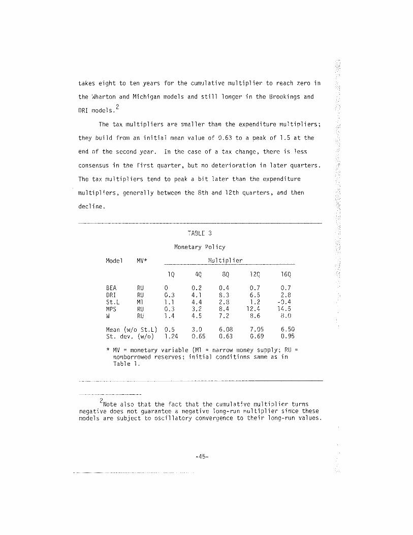
takes eight to ten years for the cumulative multiplier to reach zero in ~

the Wharton and Michigan models and still longer in the Brookings and

DRI models.2

The tax multipliers are smaller than the expenditure multipliers;

they build from an initial mean value of 0.63 to a peak of 1.5 at the

end of the second year. In the case of a tax change, there is less

consensus in the first quarter, but no deterioration in later quarters.

The tax multipliers tend to peak a bit later than the expenditure

multipliers, generally between the 8th and 12th quarters, and then

decline.

TABLE 3

Monetary Policy

Multiplier

SQ l2Q 16Q

0.4 0.7 0.78.3 6.5 2.82.8 1.2 —0.48.4 12.4 14.57.2 8.6 8.0

6.08 7.05 6.500.63 0.69 0.95

narrow money supply; RU =

conditions same as in

Model MV*

lQ 4Q

BEA RU 0 0.2DRI RU D.3 4.1St.L Ml 1.1 4.4MPS RU 0.3 3.2W RU 1.4 4.5

Mean (vito St.L) 0.5 3.0St. dev. (w/o) 1.24 0.65

* MV = monetary variable (Ml =

nonborrowed reserves; initialTable I.

2Note also that the fact that the cumulative multiplier turnsnegative does not guarantee a negative long-run multiplier since thesemodels are subject to oscillatory convergence to their long—run values.

—45—

There are only four comparable multipliers for monetary policy

(those using nonborrowed reserves). The initial quarter mean multi-

plier is small and the mean multiplier peaks at the end of the third

year at a value of 7. There is less consensus about monetary com-

pared to fiscal policy; the coefficient of variation is larger in all

but one quarter for monetary policy multipliers. While the St. Louis

cumulative multiplier peaks in the fourth quarter and goes to zero by

the 16th quarter, large scale model multipliers generally peak after 8

to 12 quarters and the MPS multiplier reported by Fromm and Klein is

still rising from the 12th to 16th quarters. The large scale models

thus suggest that monetary policy has a more persistent effect on out-

put than is the case in the St. Louis model. The exception is the DRI

model in which the cumulative monetary policy multiplier falls to zero

by the 20th quarter.

While the multiplier results do differ across models there is

clearly considerable consensus particularly over the first two years in

the case of fiscal policy when we exclude the St. Louis results. The

problem is evaluating how much divergence in the multipliers is con-

sistent with using the models for policy recommendations. Later we

will discuss the use of stochastic simulations which allow for multi-

plier uncertainty within a particular model, Here we want to note the

valuable approach suggested by Chow (1977). Chow notes that while

policy recommendations derived fron alternative structural models

differ from each other, they may nevertheless be closer to each other

than to a passive policy of constant growth rates in the policy instru-

ments. The comparison Chow suggests and implements is the improvement

in economic performance in one model using optimal policy derived from

-46—

a second model relative to the economic performance under passive

policy. Chow uses the multiplier properties of the Wharton and Michi-

gan models to construct reduced-form equations for real and nominal GNP

including government expenditures and nonborrowed reserves as the

policy instruments and employs a conventional quadratic loss function

involving deviations in real and nominal GNP from their targets (in

each case average historical values over the period in question).

The results of this experiment are mixed. If the Michigan model

were the true structure and the policy recommendations were derived

from the Wharton model, active policy would improve performance rela-

tive to a passive policy; costs under the active policy would be under

25 percent of those under a passive policy although they would be 70

percent greater than if the policy were derived using the true struc-

ture. On the other hand, if the Wharton model were the true structure

and the policy recommendations were derived from the Michigan model,

the cost under an active policy would be three times the cost of a

passive policy and about 17 times the cost when the true model was

used. And, of course, the Michigan and Wharton multipliers are quite

close at least for fiscal policies, compared to say the Brookings and

the St. Louis models. Thus there are other comparisons that would lead

to even less favorable results for activism.

A Comparison of Policy Multipliers Over Time

We expected to find a secular decline in the value of fiscal

multipliers and a secular rise in monetary policy multipliers for large

scale econometric models from the late ‘SOs versions to the versions of

the mid- to late ‘70s. However, published information on such

—47-

multipliers is relatively scarce and what is available is frequently

not constructed on a comparable basis. This, of course, increases the

value of the NBER/NSF model comparison studies but makes multiplier

comparisons pieced together from the literature hazardous. Perhaps the

most serious problems for comparing multipliers across nodels or over

time are differences in initial conditions and differences in the spec-

ification of policy instruments, particularly for monetary policy. The

large scale models are invariably nonlinear, implying that their multi-

pliers are sensitive to initial conditions, particularly the degree of

economic slack. But there is painfully little reported evidence of the

degree of this sensitivity. There are a bewildering number of possi-

bilities for a change in tax rates and even differences in nultipliers

for different government expenditure components. The most serious

problem, however, may be differences in assumptions about the monetary

policy instrument. Monetary policy, particularly in the late SOs ver-

sions, has been identified with changes in short—tern interest rates.

In other cases, monetary policy is identified with either the money

supply or some reserve aggregate, most often nonborrowed reserves. The

choice affects both monetary and fiscal multipliers since fiscal multi-

pliers assume unchanged monetary policy; fiscal multipliers will, of

course, be much larger under fixed short-term interest rates than under

fixed values of the money supply or nonborrowed reserves.

In Tables 4 and 5 we have pieced together some policy multipliers

for alternative versions of Michigan, Wharton, and MPS models. The

Michigan ‘70 and Wharton ‘68 models assume constant short—term interest

rates while the others assume constant unborrowed reserves. It is sur-

prising (to us at least) that the fiscal multipliers in the late ‘60s

-48-

TABLE

4

Real

Non

Defense

Gove

rnme

ntEx

pend

itur

eMu

ltip

lier

s-

Real

GNP

QMi

chig

an70

aMichigan

75b

Wharton

68c

Wharton

75b

Wharton

79d

MPS

69e

MPS

75b

1.5

1.4

2.0

1.3

1.1

1.3

1.2

42.

11.

72.0

2.0

1.7

1.8

2.2

81.

91.

42.0

2.3

1.8

1.6

2.2

12n.a.

1.0

2.1

2.6

1.7

1.1

0.7

a

aS.

H.Hynans

and

H.T.

Shapiro,

“The

DHL-III

Quarterly

Model

ofth

eU.S.

Economy,”

Research

Seni

nar

inQuantita

tive

Economics,

University

ofMichigan,

1970,

Table

4,p.

22.

bC.

From

nan

dL.

R.Klein,

“The

NBER/NSF

Mode

lComparison

Seminar:

AnAnalysis

ofResults,”

inL.

R.Klein

and

E.Burm

eist

er(e

x),

Econ

omet

ric

Mode

lPe

rfor

manc

e,Pennsylvania,

1975,

Table

6,p.

402.

cM.

K.Evans

and

L.R.

Klein,

The

Wharton

Econometric_Forecastjj9j~o4~j,Econonics

Research

Unit,

University

ofPe

nnsylvania,

2nd

ed.

,19

68,

Table

5,p.

SB.

dUnpublished

Whar

ton

mult

ipli

ersi

mula

tion

skindly

provided

byR.

M.Young,

Wharton

Econometrics

Fore

cast

ing

Asso

ciates.

eF.

DeLe

euw

and

E.M.

Granlich,

“The

Channels

ofMonetary

Policy,”

Federal

Reserve

Bulletin,

June

1969,

Tabl

e4,

p.489.

Shock

applied

fully

tofederal

real

wage

payments.

versions of the three models (including the two with constant short—

term rates) are so small; they peak at 2.0 or less. One important

difference in the later versions of Michigan and MPS models is the

sharp decline in the cumulative multiplier from its peak value by the

12th quarter. There was a tendency in earlier versions for multipliers

to stabilize at about 1.5—2.0 for a longer period. This continues to

be the case in the Wharton model; in both the ‘75 and ‘79 versions the

fiscal multipliers are stable or rising during the first three years.

We have been able to find comparable unborrowed reserves multi-

pliers at different points in time for only two models: the Wharton

model and the MPS model. These are reported in Table S. In these

models there is a fairly dramatic evolution of the nonetary policy

multiplier. In the 1968 Wharton model the unborrowed reserves multi-

plier for real GNP reached a fairly constant level in the 1.5 to 2.0

range after about one year. In the MPS model the multiplier is stable

in the 10.0 range during the second and third years. In the later

TABLE 5

Unborrowed Reserve Multipliers(Real GNP/Nominal Reserves)

Wharton 68c Wharton 75b Wharton 79d MPS 69e MPS 75b

1 0.0 1.4 1.2 0.7 0.34 1.5 4.5 4.8 5.4 3.28 2.1 7.2 9.1 10.0 8.412 1.7 8.6 13.3 12.4 9.4

Notes — See Table 4.

— So -

,ersions of both models, the multiplier is continually growing over the

First three years. Note also the substantial increase in the size of

the monetary policy multipliers in the Wharton model from the ‘68 ver-

sion to the ‘75 and ‘79 versions. We view the Wharton ‘68 multipliers as

fairly typical of the conventional wisdom of the mid- to late ‘SOs,

prior to the development of the MPS model.

COMMENTS ON THE “ST. LOUIS” EQUATION

Since the original Andersen-Jordan article (1968) (AJ) that pro-

posed a single equation test of the relative importance of monetary and

fiscal policies on nominal GNP, nunerous replications have been per-

formed, across time, across countries, and across functional forms and

a number of criticisms, mostly statistical in nature, have been levied

against the equation. The purpose of this section is to review the

criticisms that have been raised against the equation and to evaluate

how robust the equation appears to be against these criticisms.

The conclusions of the Andersen-Jordan investigation are by now

almost universally known. The conclusion that remains most controver-

sial is the zero cumulative fiscal multiplier for nominal GNP. This

conclusion did not conform well to the conventional wisdom of the late

1960s, nor was it consistent with other econometric results. Conse-

quently, for the past decade there has been considerable skepticism of

the specification that yields this conclusion.

Time Periods, Functional_Forms, and_Distributed_Lags

The Ad equation was estimated over the period 52/1-68/Il and sub-

sequently reestimated by Andersen and Carlson (1970) (AC) over the

53/1-69/TV period as part of the St. Louis model. In each case

—51—

monetary policy had a powerful and significant effect while the tax

variable (change in high employment receipts) was insignificant and ex-

cluded from their preferred regression and the government expenditure

variable had only a small and transitory effect. Silber (1971) subse-

quently split the period into Republican (53/I-60/IV) and Democratic

(61/I—69/IV) administrations and found that fiscal variables were sig-

nificant in the latter but not in the former. Silber argued that these

results are consistent with the more systematic use of fiscal policy in

the latter period. At a minimum, these results suggest that the time

period used in the estimation can dramatically affect the conclusions

and that the estimates may reflect the particular policies pursued over

the estimation period.

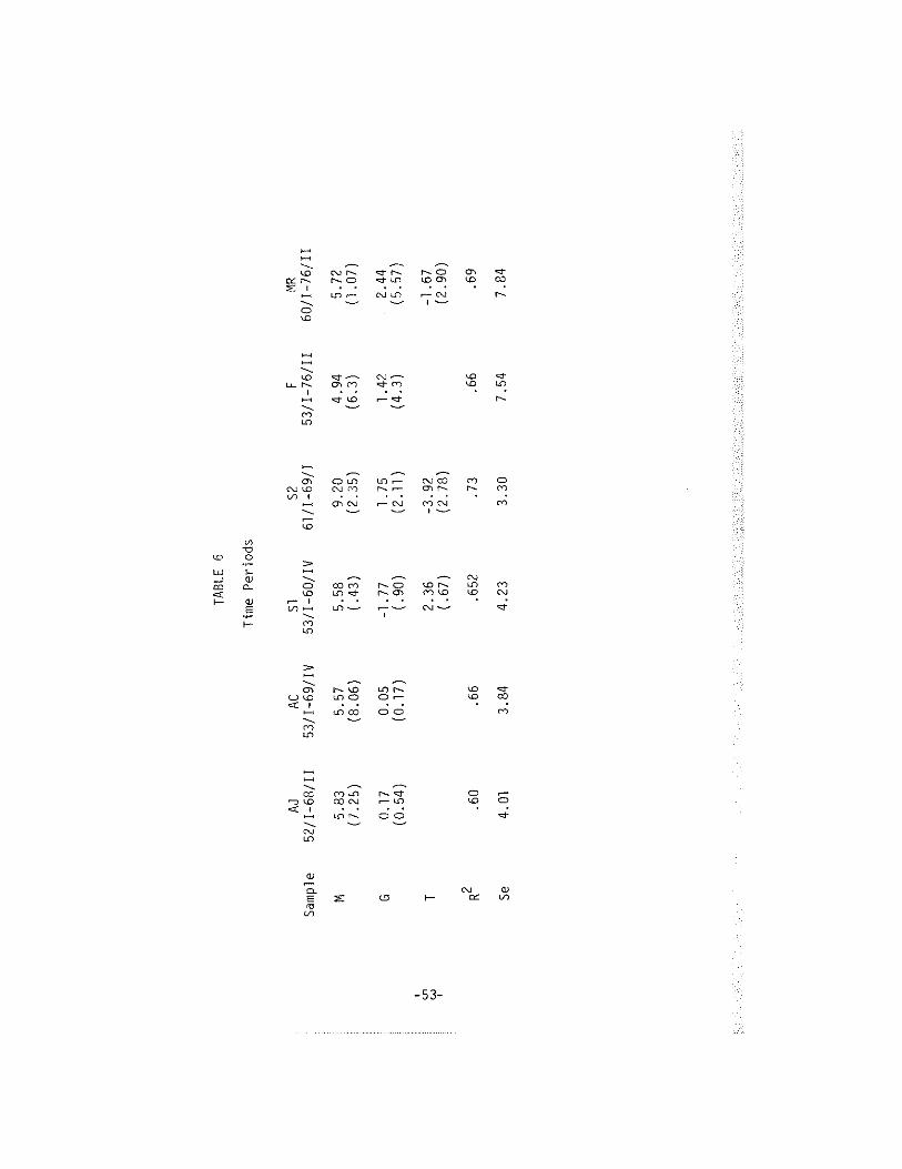
More recently Friedman (1977) has extended the sample period

employed by AC through 76/Il and concluded that “even the St. Louis

equation now believes in fiscal policy.” In Table 6 we report the re-

sults of the Ad and AC equations along with estimates over alternate

time periods including Silbers two subperiods (Sl and S2), Friedman’s

extended period (F), and the period 1960/1—1976/Il (MR). The results

suggest that both money and the time period matter~ The size and sig-

nificance of fiscal policy multipliers is not definitely settled by

these results.

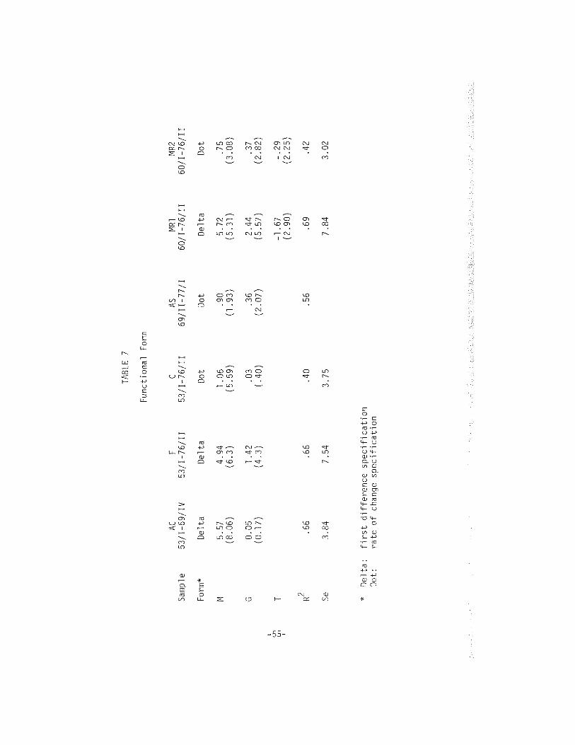
In response to Friedman, Carlson (1978) has pointed out that the

first difference form of the estimated equation, while appropriate over

the AC period, is not appropriate over the longer period because of

heteroskedasticity, implying that the t values of coefficients reported

by Friedman are unreliable. When all variables are defined as rates of

change, Carlson finds that the results of the two periods are

—52-

TABLE

6

Time

Periods

AJAC

5152

FMR

Samp

le52

/1—6

8/Il

53/I

—69/

IV53

/I—6

0/IV

61/1—69/I

53/1-76/Il

60/1-76/11

M5.83

5.57

5.58

9.20

4.94

5.72

(7.25)

(8.06)

(.43

)(2.35)

(6.3

)(1,07)

G0.17

0.05

-1.77

1.75

1.42

2.44

(0.54)

(0.17)

(.90

)(2.11)

(4.3

)(5.57)

T2.36

-3.92

-1.67

(.67

)(2.78)

(2.90)

.60

.66

.652

.73

.66

.69

Se4.

013.

844.

233.

307.

547.

84

consistent with the hypothesis that the specification is stable and,

like the original AC equation, indicate that any effect of government

expenditures is small and temporary. Allen and Seaks (1979), using the

growth rate specification, find that the fiscal variable sums to zero

in both Silber subperiods (Eisenhower and Kennedy-Johnson) but is sig-

nificant in the Nixon—Ford era (69/11-77/I). Over the period 60/1-76/Il

we find that both expenditure and tax variables enter significantly

into both first difference and rate of change specifications. In Table

7 we report the results of the AC equation in difference form over both

the original period (AC) and over Friedman’s extended period (F) and in

rate of change form over Friedman’s extended period (C) along with the

Allen-Seaks results over the Nixon-Ford period (AS) and both functional

forms over the 1960/1—76/Il period (MR1 and MR2). From these results

we can conclude that money, time period, and functional form matter.

The results of Ad type equations are estimated using polynomial

distributed lags. This technique requires selection of lag length,

degree of polynomial, and end point constraints. Schmidt and Waud

(1973) caution that introduction of inappropriate constraints can

result in biased and inconsistent estimates and demonstrate how changes

in degree of polynomial and end point constraints can substantially

alter the conclusions about policy multipliers. Others have found

length of lag can affect conclusions also.

We can conclude, therefore, that the choice of time period, func-

tional form, and lag constraints matters a great deal. The results for

money appear very robust. The results for fiscal policy are dramati-

cally affected by these factors.

-54-

TABLE

7

Functional

Form

ACF

CAS

MR1

MR2

Sample

53/T-69/IV

53/1-76/11

53/1-76/lI

69/11—77/I

60/1-76/Il

60/1-76/Il

Form*

Delt

aDelta

Dot

Dot

Delta

Dot

M5.57

4.94

1.06

.90

5.72

.75

(8.06)

(6.3

)(5.59)

(1.93)

(5.31)

(3.08)

O0.

051.42

.03

.36

2.44

.37

(0.17)

(4.3

)(.

40)

(2.07)

(5.57)

(2.82)

T-1.67

-.29

(2.90)

(2.25)

F2.6

6.6

6.4

0.5

6.6

9.4

2

Se3.84

7,54

3.75

7.84

3.02

*Delta:

firs

tdiffer

ence

specification

Dot:

rate

ofch

ange

specification

Biases Associated With Choices of Independent Variables

The inconsistency between the Ad/AC reduced-form multipliers and

the multipliers in large—scale econometric models generated a search

(on both sides of the controversy) for an explanation. Monetarists

criticized large-scale econometric models for failing to capture the

crowding—out phenomenon through misspecification of the money demand

equation (e.g. excluding a wealth effect) and failure to explicitly in-

clude a government financing constraint. The income expenditure

counterattack focused on the unreliability of reduced—forms due to a

variety of problems, some more easily correctable than others, associ-

ated with the choice of independent variables. The key issues have

been: What are appropriate measures of the policy instruments? How

can the possibility of reverse causation be avoided? What biases are

introduced by omission of nonpolicy exogenous variables?

The Measurement of Policy Instruments

There are two interrelated problems with specifying the policy

instruments. The first is the problem of specifying the instrument

that the policy authority directly controls. For example, if the Fed

sets policy by controlling the value of the monetary base, employing a

monetary aggregate other than the monetary base as a proxy for the

policy instrument may bias the policy multipliers if the other aggre-

gate varies endogenously relative to the base. A second problem arises

even if the instruments themselves are included if policy itself sys-

tematically responds to economic developments. In this case, the

policy instruments themselves become endogenous and reverse causation

again may bias the multiplier results. In this section we take up the

—56—

problem of specifying the policy instruments and in the next the

problem of endogeneity of policy.

The problem of reverse causation was noted in a DeLeeuw-

Kalchbrenner (1969) comment on the Ad paper. Indeed it was the concern

over this issue that arose out o~the Friedman-Meiselman debates that

motivated the choice of the high employment fiscal policy measures by

Andersen and Jordan. DeLeeuw and Kalchbrenner’s main concern is with

the choice of the monetary base or money supply as the variable the Fed

directly controls. They point out that the choice among the monetary

base, the nonborrowed base, total reserves, and nonborrowed reserves

depends on whether the Fed offsets the effect of movements in member

bank borrowing on the base and of movements in currency holdings on

reserves. They express no special preference among these alternate

measures suggesting only that results which hold for some measures and

not for others should be viewed with great caution. Their empirical

results indicate that fiscal multipliers are affected by the choice of

monetary instrument; in particular, fiscal multipliers of approximately

the size produced in the MPS model result when nonborrowed reserves are

substituted for the monetary base.

The treatment of fiscal instruments in the Ad/AC equations has

also drawn considerable comment. In order to avoid the bias associated

with the income induced movements in tax revenues and expenditures

(mostly transfer payments) under preexisting schedules of tax and

transfer rates, the Ad/AC equations use high employment expenditures.

High employment receipts were tried but dropped from the preferred

equation due to lack of significance. The high employment surplus was

also employed in an alternate specification.

—57—

The latter is clearly an inappropriate measure of stimulus asso-

ciated with fiscal actions because it groups components which are ex-

pected to have different multiplier responses. The same problem arises

even in the case of high employment expenditures because this variable

includes both expenditures on goods and services and transfers while

economic theory suggests that transfers should be netted against taxes.

Suggestions for improved specification of fiscal variables have been

made by DeLeeuw-Kalchhrenner (OK), Gramlich (1971), and Corrigan

(1970). Gramlich employs government purchases of goods and services

rather than high employment expenditures, and assumes no adjustment is

necessary to purge it of effects of changes in income. Government ex-

penditures are employed in a composite variable including grants—in—aid

and exports with an adjustment introduced for defense inventory

accumulation.

DeLeeuw and Kalchbrenner suggest adjusting high employment

receipts to purge changes in this variable of the effects of endogenous

movements in prices. Gramlich uses high employment net tax revenues

(taxes minus transfers) also adjusted along lines suggested by DK. The

difficulty with all these series for tax revenues is that the series

for changes include nonzero entries in periods during which no changes

in tax rates or transfer programs occurred. Corrigan has suggested an

alternate tax variable, the initial stimulus measure, that indicates

the tax revenues released or absorbed by tax rate changes. This series

has plenty of zeros~ For each tax, the initial stimulus measure is the

change in tax rates times the lagged tax base. An unweighted sum for

all taxes is the variable Corrigan used and it continues to be used in

the New York Fed version of the St. Louis equation.

-58-

The discussion above suggests that the simple specification of

both monetary and fiscal instruments employed in the Ad and AC equa-

tions may be improved upon and that such improvements might alter the

relative importance of monetary and fiscal multipliers. However, the

modifications suggested above have not generally resulted in dramatic

changes in the estimated multipliers in simple reduced—form equations.

While many of these suggestions seem valid, they have not helped to

resolve the differences between the St. Louis equation and econometric

model s.

Endogeneity of Policy

Even if we obtain measures of direct policy actions, our esti-

mates of their effects will be biased if these actions themselves are

systematically related to economic developments. This problem has

widely been noted in comments on the Ad equation, but most critics in-

cluding DeLeeuw and Kalchbrenner considered the problems in measuring

the instruments the more likely source of bias. The biases associated

with endogenous policy are easy to illustrate. If a policy instrument

varies in response to disturbances so as to eliminate completely the

instability in income, the regression of the change in the policy vari-

able on changes in income (zero by assumption) will yield a zero coef-

ficient on the policy instrument. Thus, endogeneity of policy may

result in a downward bias in the policy multiplier, with the downward

bias a funucion of the effectiveness of policy. We can, therefore,

interpret the zero multiplier on fiscal instruments as evidence of

their effectiveness rather than of their insignificance~ While the

endogeneity of policy may introduce biases into the estimates of policy

—59—

multipliers from both reduced-form equations and structural models,

Goldfeld and Blinder (1972) suggest on the bases of simulation results

that the bias is much more serious for reduced-forms. If policy

responds to economic developments with a lag, the bias is reduced but

not eliminated.

Omitted Exogenous Variables

The third major source of bias in the choice of independent

variables in the Ad/AC equation is alleged to be the omission of non—

policy exogenous variables. Andersen and Jordan explained in an ap-

pendix to their original paper why they believed that the omission of

other exogenous variables did not bias their measured impact of the

monetary and fiscal policy variables: these variables are presumed to

be independent of monetary and fiscal policies and their average effect

is registered in the constant term. Modigliani (1971) made the first

detailed critique of the St. Louis reduced-form model on the grounds of

omitted variables and Modigliani and Ando (1976) reported a more ex-

tensive set of simulation results supporting their view that omission

of exogenous variables may severely bias the results of reduced forms.

The ingenious simulation experiments involved estimation of an

Ad type equation on data generated by non—stochastic simulations of a

model. The model represents the known structure of a hypothetical

economy. The simulated values of nominal income from the model are the

“actual” values of income in the hypothetical economy. A reduced-form

is estimated using these simulated values for income, and the resulting

estimated multipliers are compared with their “true” values (the values

implied by the structural model). The comparison of the reduced—form

-60-

multipliers with their “true” (structural model) values tests the

ability of simple reduced—forms, including only a couple of policy in-

struments, to replicate the true value of the policy multipliers.

In the 1971 paper, Modigliani emphasized the finding that the

estimate of the St. Louis equation on MPS simulated values yielded a

money multiplier in excess of the “true” MPS multiplier and reached the

“unequivocal conclusion” that reduced-form money multipliers are upward

biased. This bias was attributed to positive correlation between the

money supply and omitted exogenous variables. For example, if the Fed

attempts to stabilize interest rates (as monetarists assert they often

do), then the money supply will be positively correlated with real

sector exogenous demand variables and the monetary policy multiplier

can be expected to be biased upward.

Modigliani and Ando (1976) turned their attention to biases in

the estimates of fiscal effects and suggested that correlation between

omitted exogenous variables and fiscal instruments in this case might

account for the small size and transitory effects of fiscal instruments

in the St. Louis equation. Estimates of the Ad type equation on values

of the change in nominal income based on simulations with the MPS model

yield fiscal multipliers like the original Ad equation and contrary to

the structure of the MPS model. They concluded that the St. Louis

approach is “a severely biased and quite unreliable method of esti-

mating the response of a complex economy to fiscal and monetary policy

actions” (p. 42).

To demonstrate the role of omitted variables in the bias in the

Ad equation, they remove any correlation between policy instruments and

nonpolicy exogenous variables in the structural models by assuming all

—61—

nontrended exogenous variables are constant at their means and all

trended exogenous variables grow along a constant trend. The predicted

value of nominal income for this adjusted structure is computed and

used to reestimate the Ad equation. Fiscal multipliers now of appro-

priate size and magnitude confirm the crucial role of omitted exogenous

variables in biasing the estimates of the policy multipliers in the

initial Ad equation.

In both papers, Modigliani and Modigliani and Ando (MA) are care-

ful to note that the evidence they present does not permit them either

to accept the MPS multipliers or reject the St. Louis ones. But their

results should make those who use St. Louis type reduced-form equations

uneasy about the validity of the multiplier results, particularly those

for fiscal instruments.

While the analysis demonstrates that omitted variable bias may be

a source of serious inferential error in the impact of policy actions,

the conclusion appears to be nonconstructive in the sense that it does

not provide any evidence on the particular source of the bias in the

experiments that were conducted and it suggests abandoning the entire

approach without attempting to investigate the issue of biases in the

St. Louis results directly. It would be useful to identify the sources

of bias in the estimated multipliers by introducing the most important

exogenous variables directly into the reduced-form equation.

A number of studies have attempted to address the alleged biases

in the St. Louis approach directly by including nonpolicy exogenous

variables. Gordon (1976), fur example, added a “shock proxy,’ con-

sisting of the sum of net exports, consumer expenditures on automobiles

and non—residential fixed investment to the St. Louis specification.

-62—

Although monetary multipliers decline and fiscal multipliers increase

over his longer sample period, the multiplier results with and without

the shock proxy remain qualitatively alike; monetary multipliers are

significantly positive while the sum of the lag coefficients on the

government expenditure variable is not significantly different from

zero.

Recently, Dewald and Marchon (1978) have estimated expanded St.

Louis equations for six different countries, including the United

States. They included exports as a separate independent variable, dis-

missing the conglomerate variable constructed by Gordon as including

too many endogenous influences. For the United States, the Gordon

result is replicated; the impact of monetary policy is reduced, the im-

pact of fiscal policy is left essentially unchanged, and the exports

variable has a significant contemporaneous impact. A major monetarist

contention is that the influence of a maintained change in the monetary

growth rate should be a proportional change in the growth rate of nom-

inal income. This hypothesis is alleged to be a universal phenomenon.

However, while Dewald and Marchon cannot reject this hypothesis for the

U.S. data, the monetary response for the U.S. is the strongest of any

of the six countries investigated. The long-run elasticities of nom-

inal GNP with respect to the money stock in the other five countries

never exceed .5. In France they found this elasticity to be only .07

and in two countries (France and the U.K.) this estimated elasticity is

not significantly different from zero.

-63—

Resolvjflq hePuzzleLReduced—Fonn Versus Structural Model MultiDl4~!_

Two further tests by Modigliani (1977) attempt to resolve the

puzzle of conflicting multiplier results. First of all, he suggests

that despite the apparent large differences in the AC and MPS multi-

pliers, the two sets of multipliers may not be ~ differenU

To test for significance of the difference in multipliers, Modigliani

presumes that the MPS multipliers are the true ones and tests whether

the AC multipliers differ significantly from the MPS multipliers. The

result is that they are not significantly different at the Si) percent

level. Modigliani concludes, “This test resolves the puzzle by showing

that there is really no puzzle: the two alternative estimates of the

expenditure multipliers are not inconsistent, given the margin of error

of the estimates. It implies that one should accept whichever of two

estimates is produced by a more reliable and stable method, and is

generally more sensible. To me, these criteria call, without question,

for adopting the econometric model estimates.” (p. 10)

For those who would still opt for the reduced-form multipliers,

Modigliani compares the post-sample prediction performance of the AC

equation with one in which the coefficients of government expenditures

plus exports were constrained to equal those based on multipliers de-

rived from simulations with the MPS models. The post sample simulation

begins in 197011. For the first four years, the MPS based equation

dominates: the AC equation yields “distinctly larger” errors in eight

quarters, smaller errors in only three quarters, and results in a

squared error l/3 larger than for the MPS based equation. Over the

next two years, both equations perform “miserably” but the MPS based

equation is still “a bit better.”

-64-

Conclusion

The income expenditure counterattack on reduced-forms, particu-

larly the Modigliani-Ando results on the implications of omitted exoge-

nous variables, and the ability to dramatically alter the fiscal policy

multipliers by choice of time period and functional form, have substan-

tially weakened the case based on reduced—form equations for small and

transitory fiscal effects on nominal income. The implied monetary

policy multipliers, on the other hand, have proven robust, at least for

the United States.

ASSESSING THE CUMULATIVE OUTPUT LOSS OF ERADTCATING INFLATION

A prominent policy issue of the ‘70s and one that seems certain

to dominate at least the early ‘SOs is the appropriate policy response

to a prevailing high rate of inflation. The view that there is a long—

run trade—off between inflation and unemployment, widely held at the

end of the ‘60s, is now held by only a small minority. The key issues

are the nature of the short—run relation between inflation and unem-

ployment and the process by which economic agents form inflation ex-

pectations. Macroeconomic models, both income expenditure and none—

tarist versions, suggest that while the traditional demand management

techniques remain quite capable of reducing the rate of inflation, the

cost of such a policy in terms of cumulative output loss would be

great. Despite the importance of the issues, there is substantial dis-

agreement about the cost of eradicating inflation and little evidence

on the benefits derived as a consequence.

In this section we present evidence on the cumulative output loss

associated with reducing inflation based on both estimated Phillips

-65-

curves and monetarist models. Then we discuss the most serious limita-

tion of these results -- the failure to allow the results to be influ-

enced by the degree to which the public believes policy authorities are

committed to a consistent anti—inflation policy. In the final analysis,

the cost of anti-inflation policies in the form of output loss must be

balanced against the benefits associated with a reduced rate of infla-

tion. Empirical evidence on the cost of inflation and hence the bene-

fits of reducing inflation is quite limited. Our discussion of the

benefits of anti-inflation policies is therefore confined to deter-

mining how large the per period gains would have to be in order to

justify incurring the cumulative output loss which we calculated from

the Phillips curves and monetarist models.

Econometric Evidence on the Size of the Cumulative Output Loss

Three alternative sources of evidence on the cumulative output

loss associated with the use of demand management policies to moderate

inflation are discussed below. The first is evidence directly from

estimated Phillips curves. Here we calculate how long unemployment

must be increased by either 1 percentage point or 3 percentage points

above the rate consistent with steady inflation to reduce inflation by

7.5 percentage points. The second and third sources use monetarist

models whkh include either a Phillips curve or a reduced-form equation

relating inflation to monetary change. Here we simulate the effects on

inflation and output of a phased deceleration in monetary growth.

Results Based on Estimated Phillips Curves

Three recent studies have considered the cost of reducing infla-

tion in the context of traditional Phillips curve regressions (Perry

—66-

(1978), Okun (1978), and Cagan (1978)). Perry’s results are based on a

wage change equation using the inverse of his weiqhted unemployment

rate and lagged wage change estimated using annual observations over

the 1954-77 period. His preferred equation yielded a ‘nonaccelerating

inflation rate of employment (NAIRU) of 4.0 in terms of his weighted

unemployment rate (corresponding to about 5.5 percent in the official

unemployment rate in ‘77):

(1) Mn W = -1.88 + 7.44 (1/Uw) + 0.79 A1nW1 + 0.21 A1nW2 + 1.07 ONIX

(—2.2) (3.5) (4.6) (1.1) (2.9)

S.E. = 0.70

where W = adjusted hourly earnings in the private nonfarm sector and

DNTX is a dummy for the controls equal to —1 in 1972 and 1973 and +1 in

1974 and 1975.

Any unemployment rate in excess of the critical unemployment

rate, if maintained long enough, will permit a cycling down of infla-

tion. To compute the cumulative output loss of eradicating inflation,

we begin with Mn P set equal to 10.0 in the two lagged years and at

NAIRU. Our moderate’ policy consists of increasing the weighted unem-

ployment rate 1.0 point above NAIRU in period 1 and holding it here

until ~1n P declines to 2.5, the rate presumed equal to trend growth in

labor productivity and, therefore, consistent with price stability.

The wage inflation rate falls from 10.0 to 9.6 percent in the first

year and declines about 0.3 percentage points per year thereafter

taking 23 years to reach a 2.5 percent rate. An alternative radical

policy is modeled as a 3 percent point increase in unemployment begin-

ning in period one and again sustained until wage change declines to

—67—

2.5 percent. This takes ~k 11 years: Note that the nonlinearity in

Perry’s wage equation ensures that the cumulative excess of person

years of unemployment and, hence, cumulative output loss will be

greater in the more radical policy case.

Using Okun’s estimate of 3.2 as the impact on output of a l per-

cent point increase in unemployment, we can convert the excess unem-

ployment into output ~ One percentage point increase in unemploy-

ment reduces output 3.2 percent or $45.6 billion dollars (calculated at

1978 value for real potential GNP). The 3 percent point increase in

unemployment involves an initial year output loss of $136.7 billion.

To find the cumulative, but undiscounted output loss we assume poten-

tial output will rise at a 3.3 percent rate. This yields a cumulative

loss of $1532.6 billion for the moderate policy and $1778.0 billion for

the radical policy.4 The discounted output loss is essentially the

product of the initial year loss and the number of years required to

complete the program (not accounting for the 3.3 percent rate of growth

in potential output is the same as discounting by a 3.3 percent rate);

the discounted losses are $1047.9 billion and $1503.6 billion in the

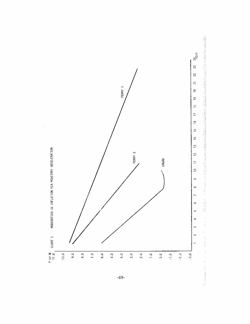
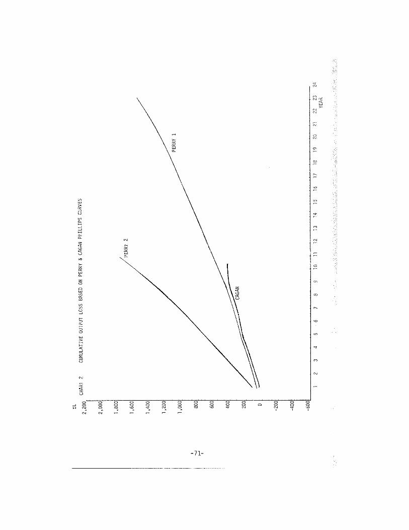
modest and radical cases, respectively. The results are depicted in

Charts 1 and 2. (Perry 1 refers to the moderate case and Perry 2 to

the radical case.)

3Estimation of the Okun law relation over more recent data sug-gests that 3.2 may be an overestimate of the output loss associatedwith a one percentage point increase in unemployment; the recent esti-mates are about 2.5.

41f the Okun’s law coefficient is 2.5 instead of 3.2, these out-put losses should be reduced by about 20 percent.

-68-

Por

Wn.

oCH

ART

1MODERATI

ONIN

INFL

ATIO

NVIAMO

NETA

RYDE

CELE

RATI

ON

10.0

9.0

8.0

7.0

6.0

5.0

4.0

3.0

2.0

1.0

0.0

-1.0

-2.0

-3.0

PERR

Y2

PERR

YI

cAGA

N

12

34

56

78

910

1112

1314

1516

1710

1920

2122

23

Okun finds that a variety of estimated Phillips curves (PC5) in

the literature yield quantitatively similar conclusions. The six

equations considered by Okun yield a first year reduction in inflation

of from 1/6 to 1/2 percentage point and an average of 0.3 percentage

points for a 1 percentage point increase in unemployment. Gramlich

(1979) reached a similar conclusion.

There are two aspects of the Perry specification which deserve

further discussion: expectations are formed adaptively and the unem-

ployment rate enters nonlinearly. The Phillips curve is uniformly

drawn as a nonlinear relation and there have been a number of theoret-

ical explanations (including Lipsey and Tobin) and some empirical sup-

port (Perry’s influential 1966 study, for example). However, nonlinear

and linear specifications seem to do about as well over sample through

the mid-197Ds.5 The existence of nonlinearity would provide a ration-

ale for the gradual as opposed to radical policy approach; the greater

the nonlinearity, the greater the cumulative output loss under the

radical as opposed gradual policy.

The inflation inertia implicit in the Perry equation derives from

two sources: actual inflation is built into expected inflation with a

lag and actual inflation responds gradually to unemployment in excess

of the critical rate. To the extent that the lag in incorporating

actual inflation into future wage negotiations is long, indexation

might substantially reduce the inflationary inertia. Even with index—

ation, there would be a lag. Assuming that the full effect occurs

5Cagan (1977) has recently noted the surprising lack of evidenceof nonlinearity and this has been confirmed in a careful examination byPapademos (1977).

—70—

ELCU

MUL

ATIV

EOU

TPUT

LOSS

BASE

DON

PERR

Y&

CAGA

NP

HIL

LIP

SCu

RVES

CHAR

T2

2,20

0

2,00

0

1,80

0

1,60

0

1,40

0

1.2

00

1,0

00

PERR

Y2

800

600

400

200

PERR

Y1

0

-200

—40

0

-600

12

34

56

78

910

1112

1314

1516

1718

1920

2122

2324

YEAR

within the first year would not dramatically reduce the cumulative out—

put costs. The cumulative output loss would decline about 20 percent

in each case. Thus, the critical determinant of the gradual decline in

inflation is the extremely small per period deceleration in inflation

associated with labor market disequilibrium (excess unemployment) in the

conventional Phillips curve, not with the slow response of inflation

expectations to changes in the actual inflation rate.

Cagan develops a PC equation beginning with the natural rate

specification and assuming adaptive expectations Cagan’s estimated PC

u—u 2 u +u(2) Pt = Pt_i - 0.95 ~ ~ ) - 0.23 ( ~ t- t-2 -

where P is the quarterly rate of change in the CPI, u is the unemploy-

ment rate for prime age males and ii is estimated from the constant of

the regression (3.7, for this regression) and the equation is estimated

using quarterly observations over the period 1953—1977.

As is clear in Charts 1 and 2, the Cagan equation generates a

dramatically more rapid decline in inflation and smaller cumulative

output loss. Beginning in period 0 at a 7.5 percent inflation rate (in

the current and last period) and at NAIRU, a one percentage point in-

crease in the unemployment rate reduces inflation by the full 7.5 per-

centage points by the eighth year with cumulative output loss of $4.2.9

billion, about a quarter of that associated with the Perry and Okun

results.

—72—

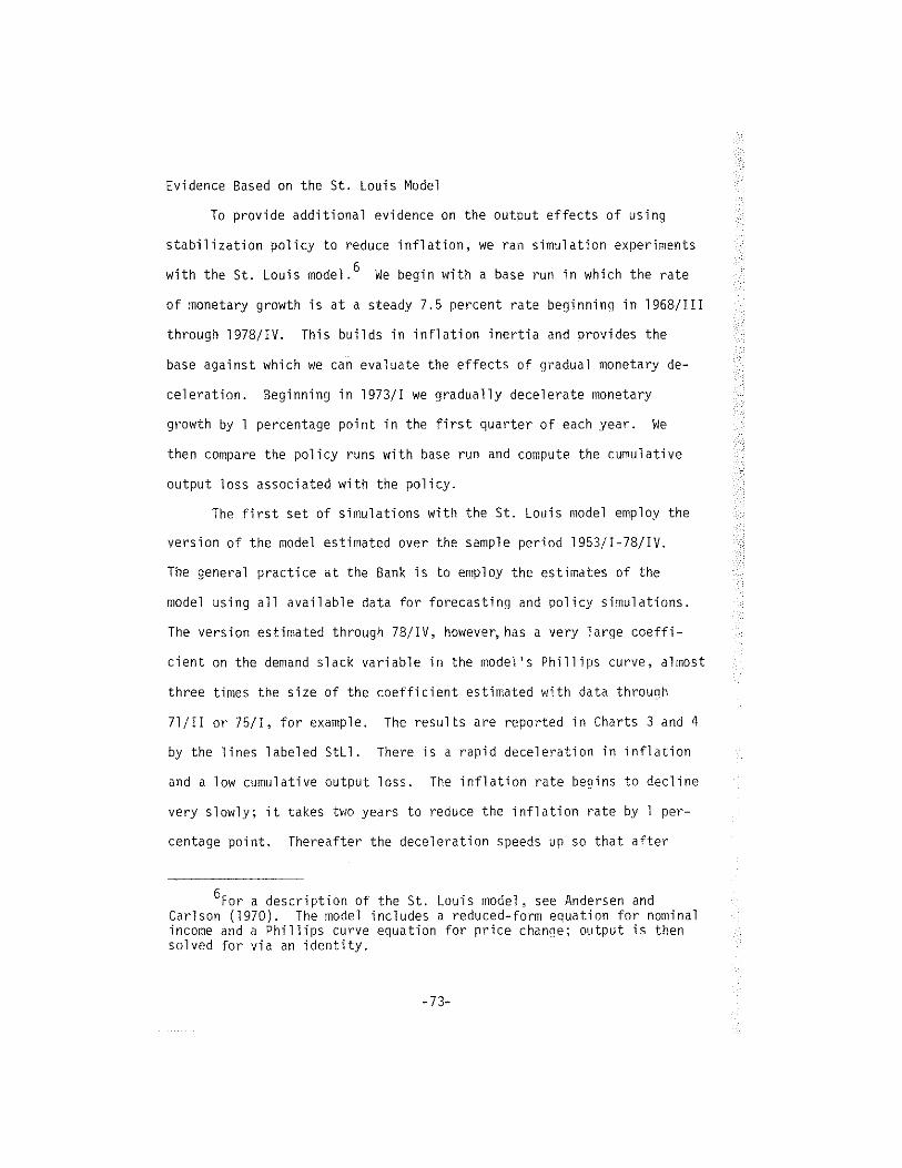
Evidence Based on the St. Louis Model

To provide additional evidence on the output effects of using

stabilization policy to reduce inflation, we ran simulation experiments

with the St. Louis model.6 We begin with a base run in which the rate

of monetary growth is at a steady 7.5 percent rate beginning in 1968/TI!

through 1978/TV. This builds in inflation inertia and provides the

base against which we can evaluate the effects of gradual monetary de-

celeration. Beginning in 1973/I we gradually decelerate monetary

growth by 1 percentage point in the first quarter of each year. We

then compare the policy runs with base run and compute the cumulative

output loss associated with the policy.

The first set of simulations with the St. Louis model employ the

version of the model estimated over the sample period l953/I-78/IV.

The general practice at the Sank is to employ the estimates of the

model using all available data for forecasting and policy simulations.

The version estimated through 78/TV, however, has a very large coeffi-

cient on the demand slack variable in the model’s Phillips curve, almost

three times the size of the coefficient estimated with data through

71/I! or 75/I, for example. The results are reported in Charts 3 and 4

by the lines labeled StL1. There is a rapid deceleration in inflation

and a low cumulative output loss. The inflation rate begins to decline

very slowly; it takes two years to reduce the inflation rate by I per-

centage point. Thereafter the deceleration speeds up so that after

6For a description of the St. Louis model , see Andersen andCarlson (1970). The model includes a reduced—form equation for nominalincome and a Phillips curve equation for price change; output is thensolved for via an identity.

-73—

5—1/2 years, inflation has declined by 7.5 percentage points. The un-

employment rate rises slowly at first and the maximum increase is only

1.8 percentage points, during the sixth year. The cumulative output

loss is only about $200 billion.

The output loss is, of course, sensitive to the coefficient on

the demand variable in the Phillips curve. Using a version of the

model estimated through 71/111, where the coefficient on the demand

variable is substantially smaller than in the first version discussed,

inflation decelerates much more gradually; after six years the infla-

tion rate in the policy run is only four percentage points below that

in the base run. At this point unemployment is four percentage points

higher than in the base run. The cumulative output loss is $350

billion at this point and escalating rapidly. These results are de-

picted in Charts 3 and 4 by the lines labeled StL2.

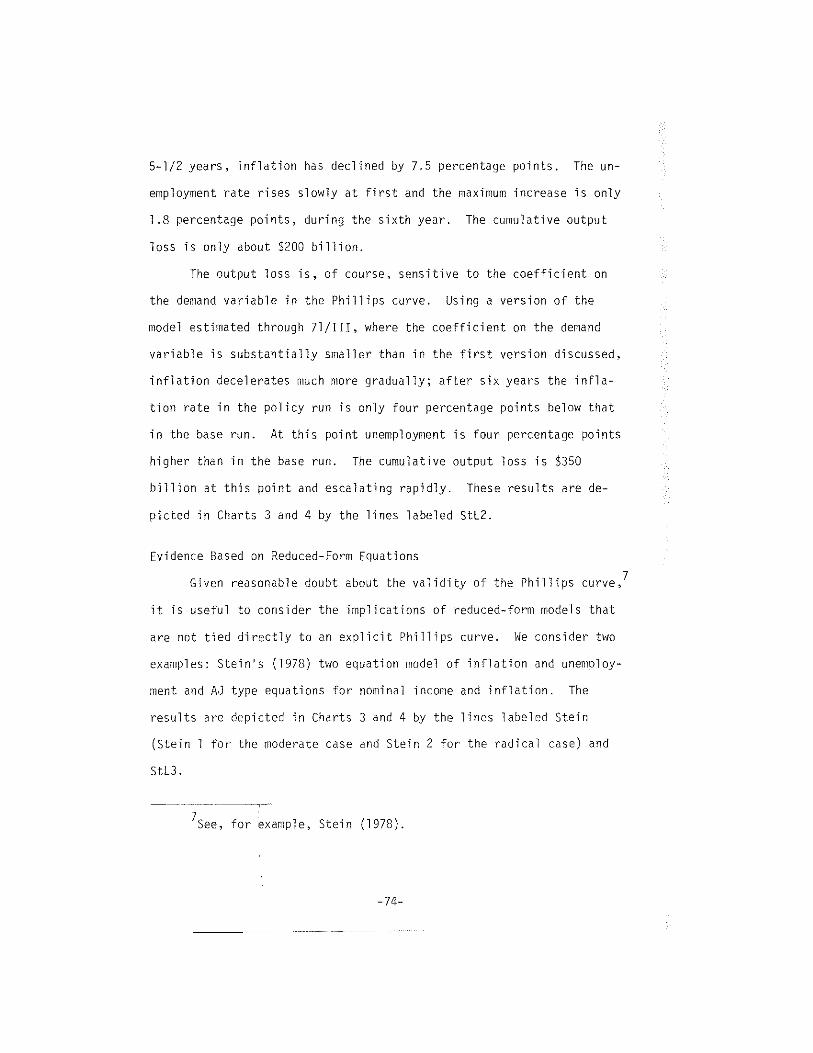
Evidence Based on Reduced—Form Equations

Given reasonable doubt about the validity of the Phillips curve,7

it is useful to consider the implications of reduced—form models that

are not tied directly to an explicit Phillips curve. We consider two

examples: Stein’s (1978) two equation model of inflation and unemploy-

ment and AJ type equations for nominal income and inflation. The

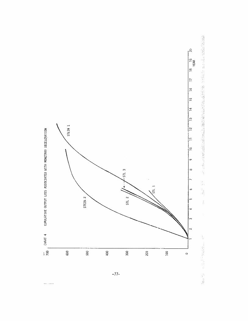
results are depicted in Charts 3 and 4 by the lines labeled Stein

(Stein 1 for the moderate case and Stein 2 for the radical case) and

StL3.

7See, for example, Stein (1978).

—74-

P

10.0 9.0 8.0

7.0 6.0

5,0

4.0

3.0

2.0

1.0 0

CHAR

T3

MOD

ERAT

ION

ININ

FLAT

ION

VIA

MONE

TARV

DECE

LERA

TIO

N

12

34

STL

2

67

STEI

NI

810

1112

YEAR

The Stein model -- In the Stein model , both unemployment and

inflation are driven by the rate of monetary growth. Stein’s two

equation model is:

(3) A u(t) = 3 - 0.6 u(t-1) + 0.4 (t-i) - 0.4 ~ (t-i)

(4) A ~t) •~04~ (t-i) + 0.4 Ul (t~i)

where u is the unemployment rate, w is the inflation rate and ~ is the

rate of monetary growth. The critical unemployment rate is 5.0 and the

equilibrium rate of inflation is the rate of monetary growth. Begin-

ning at u = 5,0 and ~(t)= +(t-l) = 7.5 = p~(t) ~~1(t-1),we decel-

erate the rate of monetary growth either (a) gradually by 1 percentage

point per year until ~ = 0 or (b) immediately to 0. In the gradual

policy, unemployment rises beginning in year 2 and peaks in year 8 at

6.6 percent returning to almost 5 percent by year 16. The inflation

rate begins to decelerate in year 2 initially at a 0.4 percent point a

year rate but ultimately reaches 1.0 point per year by year 7. The

inflation rate is down to 2 percent by year 8 and thereafter declines

gradually to about zero by year 16. The cumulative output loss is

$687.5 billion. Interestingly, the gradual policy incurs a smaller

cumulative output loss, $613 billion.

The St. Louis reduc —for~euatjonfor income with a reduced—

form for inflation —- A second simulation based on reduced-form equa-

tions combined the reduced—form for nominal income in the St. Louis

model with a reduced-form equation for inflation.8 The inflation

8The reduced-form equation for inflation used in this section wasdeveloped by Jack Tatom of the Federal Reserve Bank of St. Louis. Anearlier version of this equation was used by Tatom in “Does the Stageof the Business Cycle Affect the Inflation Rate?” Federal Reserve Bankof St. Louis Review, September 1978, pp. 7-15.

—76—

CHAR

T4

CU*JLATI

VEOU

TPUT

LOSS

ASSO

CIAT

EDWI

THNONETARY

DECE

LEMT

ION

STEIN

1

1011

1213

1415

1617

1819

YEAR

600

500

STEIN

2

400

300

STL

3

200

100

STL

1

05

23

46

78

920

reduced-form includes a twenty period distributed lag on the rate of

change in the money supply and a four quarter distributed lag on the

differential in the rate of change in producer prices for energy and

the price index for the nonfarm business sector, and two dummies for

the effects of the freeze and Phase II and for the subsequent catch up

effects. The St. Louis equation yields values for nominal income; the

inflation reduced form is employed to generate price level predictions;

and the price level is used to deflate nominal income to yield real

output predictions. The results in Charts 3 and 4 depicted by the line

labeled StL3, reflect the response to the same phased monetary deceler-

ation employed with the other St. Louis model simulations described

above.

Note the similarity with the St. Louis results with a Phillips

curve (based on the sample period through 71/Il), StL2, in Charts 3 and

4. With the reduced-form equation inflation declines more rapidly, by

about .20 - .30 percentage points per year over most of the period; cor-

respondingly, the output loss is somewhat smaller. But the time

pattern and magnitude of both the deceleration in inflation and the

cumulative output loss are remarkably similar. Again note that the

output loss per quarter has not peaked after six years of the phased

deceleration so that the cumulative output loss is still rising raoidly

at the end of six years.

Qualifications of the Empirical Analysis

The results reported above are derived both from explicit

Phillips curves, and from monetarist reduced-forms. The existence of a

cumulative output loss associated with eradicating inflation is

-78-

therefore generally consistent with both income-expenditure structural

models and monetarist reduced—forms. The major deficiency of the em-

pirical analyses on which the results described above are based is the

failure to allow the public’s perception of current and future policy

to affect expectations about future inflation.

The Credibility Effect

The results reported above based on Phillips curves all related

inflation in the current period to a distributed lag on past inflation

rates where the latter are intended to reflect the rate of inflation

expectations (and/or direct the influence of past inflation as for ex-

ample via catch—up effects). This specification does not allow the

degree of credibility associated with announced anti—inflation policies

or even the expected influence of recent policy actions to influence

inflation expectations. The estimates of cumulative output loss gen-

erated by such models are, therefore, almost certain to be over-

estimates. Fellner (1979), for example, maintains that ... the

standard model coefficients... would change significantly for the

better -- in the direction of a much more rapid rate of reduction of

inflation for any given slack -- if a demand management policy,..

changed to a credible policy of consistent demand disinflation.” But

by how much does the standard model overestimate inflationary inertia?

By 10 percent, 50 percent?

We do not have any reliable quantitative estimate of the degree

to which policymakers can speed the deceleration of inflation by

clearly defining their anti—inflation policies and convincing the

public that they intend to follow through. Nevertheless, there would

—79—

be nearly universal agreement that anti—inflation policies ought to be

set out Clearly and supported by both the Treasury and the Federal

Reserve in such a manner as to maximize the Credibility effect.

Rational Expectations and the Cumulative Output Loss

In the extreme form of rational expectations models advocated,

for example, by Sargent and Wallace (1976), the cumulative output loss

associated with a credible policy of monetary deceleration should be

zero. These models have two essential features: 1) they are equilib-

rium models in which prices respond immediately and fully to monetary

change and real variables such as unemployment and output respond only

to unanticipated inflation; and 2) inflation expectations are formed

rationally, taking into account knowledge both about the structure of

the economy and the systematic features of policy.

In such a model, inflation should moderate imediately in re-

sponse to the monetary deceleration, provided, of course, that the

policy was announced in advance and believed (or otherwise expected).

We had thought of running simulations with an RE version of the St.

Louis model along lines suggested by Andersen (1979). On a moment’s

reflection, the implications were sufficiently obvious that computer

simulations could be dispensed with. The St. Louis model has a

Phillips curve in which inflation depends on a demand variable (x) and

expected inflation (pe) where the latter is determined from an adaptive

expectations model with weights taken from a regression of the nominal

interest rate on past inflation rates:

(5) P = + Sx + ~P

-80-

Andersens RE version imposes the condition that = E(P); i.e., that

subjective inflation expectations equal the model’s forecast for infla-

tion. In this case:

(6) E(P)a+Sx+eE(P)

(6’) E (P) l~E(sx)

and Andersen substiti~tes

(7)

for the St. Louis Phillips curve.

Andersen sets ~ = .86, its value in the St. Louis model. How-

ever, if c is meaningfully viewed in this case as the coefficient on

expected inflation, the value of .86 estimated in the St. Louis model

should not be accepted as the magnitude of that parameter in the RE

version of the St. Louis model because the value of c was estimated

under the assumption that expectations were formed adaptively. Taking

= 1, as seems essential to the RE model, equation 7 no longer is a

meaningful equation for P. Instead we obtain from (6) where c =

(6’) 0 = ct + sx

so that there is a unique value of x* = — a/s corresponding, of course,

to the natural rate of unenployment. x can differ from x* only on

account of random disturbances (with zero mean). In this case any

effect of monetary deceleration on the rate of growth of nominal income

is transformed immediately and fully into a decline in inflation

without any cumulative output loss. This seems to us a more

-81-

meaningful RE version of the St. Louis model than that employed by

Andersen

Balancing the Gains from Reducino Inflation~g~jpstthe Transitional

Costs ~

The cumulative output loss is a measure of the cost of anti-

inflation policies. To evaluate the desirability of such policies we

also need to assess the gains from reducing inflation. Unfortunately,

the costs of inflation (and hence the benefits of reducing inflation)

are not as clearcut or easily quantifiable as the cost of unemployment.

Fischer and Modigliani (1978) provide a careful outline of the costs of

inflation. The costs include the welfare loss associated with the

incentive to economize on cash balances, the reduction in capital ac-

cumulation due to disincentives for saving and investment that reflect

the way in which the tax system permits inflation to affect after—tax

9There is a second and related objection to Andersen’s approach.In the St. Louis model a is not the sum of the coefficients on laggedinflation rates. Indeed the sum of the coefficients is generally about1.0. The reason for this is that the St. Louis Phillips curve does notestimate the weights on lagged inflation directly within the estimationof the Phillips curve itself. First, an equation for a short-terminterest rate is estimated as a function of the rate of monetary growthand distributed lags on both the rate of change in output and on pastinflation rates divided by the ratio of unemployment to the full—employment rate. The sum of the coefficients on lagged prices from theinterest rate equation in the original Andersen/Carlson article was1.27 so the sum of weights on lagged inflation rates in the Phillipscurve is .86 (1.27/(u/uf)), approximately 1.0. The sum of the infla-tion coefficients from the interest rate equation vary considerablyover different sample periods and the estimate of a always compensatesto yield a sum on past inflation rates of about 1 .0. This reinforcesour view that the value of a in equation (6) should be taken as 1.0.

10This section was added to the original paper and was motivated

by comments by Jerry Jordan and Allan Mel tzer at the conference.

-82-

rates of return and the cost of capital, and the arbitrary redistribu-

tion of income and wealth due to unanticipated inflation.

While Fischer and Modigliani do provide estimates of some compo-

nents of the costs of inflation, neither their study nor others permit

us to compute a meaningful estimate of the benefits that would accrue

from reducing inflation which could in turn be compared with the cost in

terms of cumulative output loss. What we can compute is the minimum

size of the permanent gain in output per year due to eradicating infla-

tion which would just justify incurring the cumulative output loss asso-

ciated with the transition to price stability. We will refer to the

benefits as a gain in real output per year. Some components of the gain

may, however, be welfare or utility gains that would not necessarily

show up in computed measures of real output. While such welfare gains

are even more difficult to evaluate than output gains, they are no less

important in developing a measure of the benefits of reducing inflation.

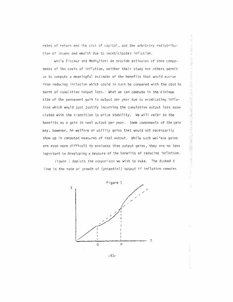
Figure 1 depicts the comparison we wish to make. The dashed X

line is the rate of growth of (potential) output if inflation remains

x —

on

Figure 1

—83-

indefinitely at 7.5 percent. If anti-Inflation policies are pursued,

output is assumed to follow the solid line. The transitional costs

occur between t = 0 and t = n as unemployment rises above the rate

associated with potential output. However, if there are costs of in-

flation, output will rise above the level that would have prevailed if

the initial steady inflation rate had continued. We define G as the

present value of the permanent per period output gain, evaluated from

period n to

(8) G = ri=n (l+r)’

This can be compared to the present value of the cumulative output loss

(L)

n—l L.(9) L = z

i0 (l+r)1

where L~ is the output loss in the ith period (i=0, . . . n—l).

Assuming that the unemployment rate is maintained above the rate

consistent with potential output by a fixed amount for n periods, the

loss in period i can be expressed as

(10) L~ E (1+p)1

where U is the loss in the first period and a is the rate of growth in

potential output. If r=p, the expression for L simplifies to

(10’) L = nTi

This is precisely the way we calculated the discounted value of the

cumulative output loss above for the Perry and Cagan equations.

-84-

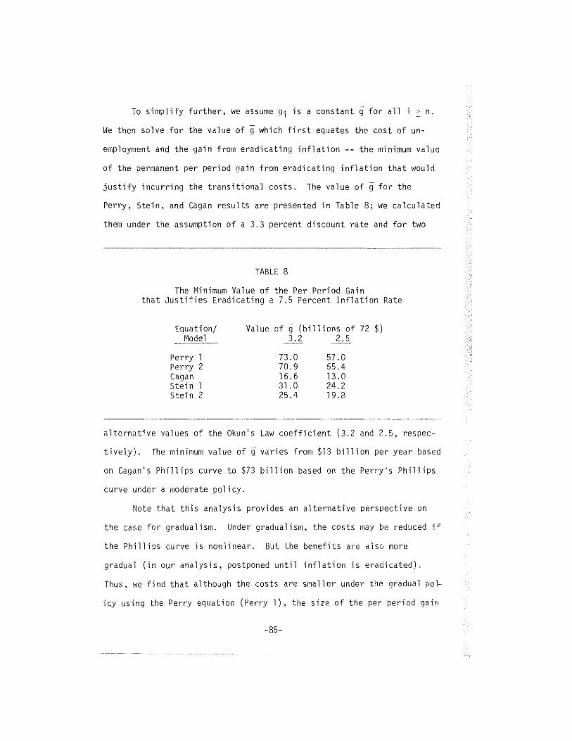
To simplify further, we assume g~is a constant ~ for all i > n.

We then solve for the value of g which first equates the cost of un-

employment and the gain from eradicating inflation -— the minimum value

of the permanent per period gain from eradicating inflation that would

justify incurring the transitional costs. The value of ~ for the

Perry, Stein, and Cagan results are presented in Table 8; we calculated

them under the assumption of a 3.3 percent discount rate and for two

TABLE 8

The Minimum Value of the Per Period Gainthat Justifies Eradicating a 7.5 Percent Inflation Rate

Equation/ Value of ~ (billions of 72 $)Model 3.2 2.5

Perry 1 73.0 57.0Perry 2 70.9 55.4Cagan 16.6 13.0Stein 1 31.0 24.2Stein 2 25.4 19.8

alternative values of the Okuns Law coefficient (3.2 and 2.5, respec-

tively). The minimum value of ~ varies from $13 billion per year based

on Cagan’s Phillips curve to $73 billion based on the Perry’s Phillips

curve under a moderate policy.

Mote that this analysis provides an alternative perspective on

the case for gradualism. Under gradualism, the costs may be reduced if

the Phillips curve is nonlinear. But the benefits are also more

gradual (in our analysis, postponed until inflation is eradicated).

Thus, we find that although the costs are smaller under the gradual pol-~

icy using the Perry equation (Perry 1), the size of the per period gain

-85-

required to justify eradicating inflation is smaller under the more

radical policy (Perry 2). The radical policy also yields a smaller

minimum per period gain using the Stein model, although this result was

expected in this case because the cost turned out to be lower in the

radical case using Stein’s model.

The calculations reported above presumed that the gains from re-

ducing inflation could be meaningfully represented as a fixed real sum

per period. What if the gains are more meaningfully specified as a

real sum which grows at the same rate as potential output? For example,

the cost of a fully anticipated increase in inflation is generally

measured by the reduction in the area under the demand curve for money

balances as wealth owners reduce their demand for money in response to

the associated rise in nominal interest rates. The decline in demand

for real money due to a rise in the interest rate is generally viewed

as proportional to the overall scale of money holdings which, in turn,

is determined by the level of transactions (e.g. real income). The

cost of a given rate of inflation and hence the benefits of eliminating

the inflation may therefore grow at the rate of increase of potential

output. In this case where ~ is the value of the gain in period n (the

(8’) G=~i=n (l+r)1

first period in which a gain is registered). For ~ > r, G ~ co. This

corresponds to the result recently derived by Feldstein (1979): if the

cost of inflation grows at a rate equal to or greater than the discount

rate, any positive initial gain (any ~ > 0) is sufficient to justify

incurring any finite transitional cost~

-86-

These results suggest that the case for anti—inflation policies

should not be dismissed lightly, even when there are large transitional

costs of eradicating Inflation. The range of the estimates of the

cumulative output loss, the uncertainty about the adjustment in those

results required to allow for the credibility effect, and the lack of a

quantitative estimate of the cost of Inflation makes it extremely dif-

ficult to make a meaningful comparison of the costs and benefits of

anti—inflation policy. It should not be surprising therefore that

policymakers generally seem indecisive and often lacking In coninitment

to reduce Inflation. Narrowing the range of estimates of output loss

and developing a measure of the cost of inflation should be high on the

priorities for macroeconomic research in the 1980s.

RULES VERSUS ACTIVISM

The case against activism rests on two propositions. The first

proposition is that the private sector of the economy is inherently

stable. This is a major tenet of monetarism and suggests the absence

of a need for stabilization policy. Indeed, monetarists generally con-

tend that the instability observed in the economy results mainly from

government rather than private sector decisions. The inherent stabil-

Ity of the private sector results In part from the absence of large and

persistent exogenous shocks and in part from the fact that the shocks

that do occur have relatively small and only temporary effects on out-

put and employment as a consequence of the economys built-in stability.

The second proposition in the case against activism is that even

if the economy were subject to cumulative movements In output, employ-

ment and inflation relative to target levels, discretionary policy

-87-

might only compound the instability rather than dampen it. The danger

that policy will turn out to be destabilizing follows from the long

inside lag, the long and variable outside lag, and the general uncer-

tainty about the effect of policy on the economy.

The case for activist policy involves a rejection of the two prop-

ositions developed above; the economy needs to and can be stabilized by

appropriate manipulation of policy instruments. The first proposition

in support of policy activism, then, is that the economy is subject to

substantial and persistent disturbances arising from the private sector.

In addition, nonmonetarists contend that policy can be implemented with

sufficiently short inside lags and with sufficient precision qiven our

understanding of the structure of the economy to yield an improvement

in economic performance relative to a policy of a fixed rule.

Relevant empirical evidence on rules versus activism includes:

(1) the relative size of exogenous impulses arisinq from

policy and nonpolicy sources

(2) the degree of persistence in the response to such

disturbances

(3) the ability of active policy to improve economic per-

formance in the face of the disturbances.

Stability of the Private Sector

The issue of the stability of the private sector has been catego-

rized as a fundamental difference between monetarists and the conven-

tional Keynesian tenets (See Andersen (1973) and Mayer (1975)).

Nevertheless, it appears to be an issue on which little, if any, rele-

vant empirical evidence is available.

The evidence that is conventionally cited in response to the

allegation that the Keynesian position regards the private sector as

-88-

inherently unstable is the result of simulation experiments with

various econometric models. These experiments suggest that the models

are stable, usually exhibiting highly damped oscillations back to

equilibrium following some shock (see Klein (1973)). Such results

under the postulated experimental conditions are probably a necessary

condition, but not a sufficient condition to substantiate the mone-

tarist proposition. We would need to look at the degree of damping

under a policy of fixed rules relative to the damping under an endoge—

nous policy with feedback from current economic developments. The case

for rules is enhanced if endogenous policy reduces the degree to which

disturbances are damped.

Evidence from Model Simulations

Discussions of the effectiveness of policies often focus on the

size of policy multipliers. Such measures of the leverage of policy on

goal variables are critical to setting policy, but do not provide any

evidence on the usefulness of discretionary policy unless they are zero.

Indeed as Cooper and Fischer demonstrate, even if the policy instrument

has a zero cumulative multiplier it may be useful as a stabilization

tool as long as it has a nonzero short-run multiplier. More important

is the pj4jç~jjit of the outcome of policy actions which is more

closely related to the errors in forecasting the goal variables. The

case for discretion, therefore, has little or nothing to do with the

size of policy multipliers, unless there is some concern about moving

the policy variables too far or too fast such as when a “penalty

function” is added to the “goal function.” The time pattern of the

response as well as the predictability of the policy multipliers, on

—89—

the other hand, do matter. Evidence on rules versus discretion, there-

fore, generally involve model simulations and these are most useful If

allowance is made for uncertainty about the multipliers.

Below we review the evidence on the comparison of economic per-

fonnance under rules and discretion based on simulations with macro-

economic models. First we must define a set of alternative policies;

four alternatives have been Investigated.

1) Actual policy: Historical simulations in which policy Instruments

take on their historical values provide the benchmark of actual policy,

discretion as it was implemented as opposed to what would have been

optimal in the context of the model under consideration.

2) FIxed rifles or rules without feedback: Simulations In which the

policy instrument is constrained to grow at a constant rate provide

evidence on the effect of fixed rules; for example, a constant rate of

monetary growth as advocated by Friedman. In this case the policy in-

strument is totally independent of current economic developments.

3) Active rules or rules with feedback: An alternative to both dis-

cretion and fixed rules is an active rule or a rule which requires

policy instruments to respond systematically to current economic devel-

opments. This approach introduces Phillips type ad hoc rules involving

proportional and derivative controls. Some experimentation is under-

taken to identify “good” rules but short of full optimization. Such

simulations can be viewed as a way of modeling systematic discretionary

policy without the blatant policy errors that in retrospect always mar

the historical runs.

4) Optimal control: The benchmark for identifying the best that is

possible under discretionary policy is an optimal control simulation in

—90-

which policymakers are viewed as selecting a time path for their in-

struments that minimizes the losses associated with deviations of their

goal variables from their target levels. It, therefore, requires im-

posing an explicit loss function including the designation of relative

weights on competing objectives and solving the model subject to mini-

mization of the losses. The solution allows the selection of an in-

strument path to reflect knowledge of the structural parameters of the

model and forecasts of future performance based on current and past

values of exogenous variables and the dynamic structure of the model.

A superior eccmomic performance under such circumstances hardly pro-

vides convincing support for discretionary policy, although it provides

evidence of tne potential for discretionary policy to improve economic

performance.

The various policy regimes can be simulated in a number of dif-

ferent ways. In a deterministic simulation the error terms in the

various estimated equations are set to zero. This immediately removes

a potentially important source of instability in the private economy

and should be expected to bias results in favor of fixed rules. There

are two basic types of stochastic simulations reflecting the two

sources of random disturbances: the additive error terms in the esti-

mated equations and the estimated coefficients. Simulations allowing

for random additive error disturbances are generally labeled stochastic

simulations while those that randomize both parameters and additive

errors are referred to as fully stochastic simulations.

—91—

Actual Policy Versus Fixed Monetary Growth Rules

Modigliani reports two simulations with a fixed monetary growth

rule over the period beginning in 1959 and ending in mid-1971. In each

case Ml is constrained to grow at a 3 percent annual rate. In the

first simulation all shocks are eliminated by substituting constant

trends or means for untrended exogenous variables. In the second, his-

torical values of exogenous variables are employed. In the first case

the monetary rule stabilizes the economy, but, allowing for historical

shocks the economy “was distinctly less stable than actual experience,

by a factor of 50 percent [p. 12].”

Eckstein investigates the implications of smooth growth in non—

borrowed reserves over the period of 1964 through 1975. (Nonborrowed

reserves grow at a 4 percent rate in ‘64, accelerate 1/4 percent point

each year until they stabilize at a 6 percent rate during and after

1972). Eckstein finds that smooth growth in reserves does result in

“a more stable growth pattern” but does not dramatically alter the

overall results for economic performance.

Active Rules Versus Fixed Rules

In a series of papers employing simulations with both the MPS and

St. Louis models, Cooper and Fischer (1972a, l972b, 1974) compare

Phillips type feedback control rules with fixed growth rate rules.

They conclude that there are active rules which dominate fixed rules

for both models, under deterministic, stochastic and fully stochastic

simulations. The dominant active rules generally involving strong

derivative controls and some proportional control. The criterion was

the average standard deviation in the unemployment and inflation rates.

—92-

For the St. Louis model, for example, the average standard deviations

for each variable were reduced by about 20 percent in the deterministic

simulations (over the period 56/I-68/IV), between 50 - 70 percent in

the stochastic simulations (over the same period) and by about 50 per-

cent in the fully stochastic simulations (over the period 55/I — 7l/IV).

The improvement was more modest, however, in the MPS model , where the

standard deviation of unemployment fell by 4 - 24 percent and that of

inflation by 7 - 32 percent in stochastic simulations over the period

1956/I — 68/IV.

Optimal Control Simulations

There have been numerous attempts to compare fixed rules with

optimal control simulations including Chow (1972), Garbade (1975),

Cooper and Fischer (1975), Crane, Ravenner and Tinsley (1976), and

Crane, Havenner and Berry (1978). The first four studies find that

fixed rules are uniformly inferior to optimal control (and generally

inferior to historical policies). These studies use stochastic simula-

tions but actual values of exogenous variables and, with the exception

of Cooper and Fischer, constant parameter values. Garbade for example

finds that “discretion,” in the form of optimal control, reduces the

expected loss by 50 percent compared to a fixed rule, a result in close

agreement with Chow. Garbade views his results as adding to the

“accumulating evidence” of the gains associated with discretion “when a

valid representation of the economy is available.” But that, after all,

is the major element in the controversy.

Cooper and Fischer find that their active rules perform quite

well in relation to optimal control solutions using the St. Louis model.

—93—

Costs are reduced by about 45 percent relative to fixed rules, but

fixed rules outperform historical policy In this case due in part to

greater instability in instrument movements in the latter case. The

Cooper—Fischer paper produces a possibly valuable insight about the

relative performance of rules and discretion. Stochastic simulation

requires multiple simulations for alternative realizations of the

stochastic disturbances. They found that the poor overall performance

of fixed rules resulted from their “spectacularly bad” performance in

replications where losses turned out to be above average for all

policies. Where average performance Is good, on the other hand, fixed

rules perform about as well as optimal control. This may imply that

optimal policy is nonlinear—restrained to fixed rules within a band

around target values of goal variables and active only outside those

bands. Thus, “fine tuning” is rejected, but activism In the face of a

major disturbance has a substantial payoff.

This conclusion is reinforced by the Crane, Havenner and Tinsley

study of the 1911/1-1974111 period using a condensed version of the MPS

model, MINNIE. Optimal policy is not especially volatile after an

initial aggressive expansionary policy in the first two quarters to

offset the recession implicit in the initial conditions. The optimal

policy again dominates fixed rules, in this case by about 40 percent;

and fixed rules would have increased expected losses by about 45 per-

cent relative to historical policies.

Rational Expectations and the Limits of Activist Policy

The traditional arguments against activist policy focused on the

Implications of long inside lags, long and variable outside lags, and

-94-

multiplier uncertainty; there was a general emphasis on the limitations

of policy in an environment characterized by insufficient knowledge of

the economys structure. The Lucas—Sargent—Wallace rational expecta-

tions models suggest a dramatically different basis for fixed rules.

These models suggest that policy is doomed to ineffectiveness in an

environment in which economic agents have knowledge both about the

structure of the economy and the way in which policy authorities re-

spond to economic developments. In this case too much knowledge rather

than too little knowledge underlies the ineffectiveness of policy.

Real variables according to these models respond only to unanticipated

price or inflation shocks. Systematic policy, by definition, cannot

produce surprises. Therefore, although there exists a trade-off be-

tween unanticipated inflation and unemployment, it cannot be system-

atically exploited by policy authorities; this is generally referred to

as the neutrality proposition. The theoretical structure of these

models and the implications of a number of qualifications, particularly

the existence of nominal contracts, have been thoroughly developed in

the paper by Taylor. The role, operational specification, and implica-

tions of rational expectations in macroeconomic models is the central

issue in macroeconomic theory today and empirical investigations of

these models is certain to be the growth industry of the SOs. There

are, however, only a handful of empirical studies to date that attempt

to test the neutrality proposition.

McCallum (1979) in a recent survey of this literature notes that

while the formal evidence is not inconsistent with the neutrality

proposition. . . the power of existing tests is not high and, in any

event, the evidence is not entirely clearcut. The two most important

-95—

empirical studies are the Barro papers (1977, 1978) on the effect of

unanticipated monetary growth on unemployment and output and Sargent’s

paper (1976) applying Sims and Granger tests for causality to movements

in the unemployment rate, the money supply, government expenditures and

other macro variables.

Barro estimates a reaction function to isolate unanticipated

monetary growth and then examines the role of unanticipated and antici-

pated monetary change on unemployment and output. His results are re-

markably one sided, supporting the hypothesis that only unanticipated

policy actions affect real variables. But his empirical methodology

has been convincingly critiqued by Small, Fischer (1978) and Gordon

(1979). Sargent is somewhat more cautious in interpreting his findings

as indicating that “the causal structure imposed on the data by the

classical model. . . is not obscenely at variance with the data [p. 233].”

We think this means the results are mixed, which indeed they are.

There is some evidence, for example, that movements in the money supply

“cause” movements in the unemployment rate (using the Granger test) and

some evidence that it does not (using the Sims test).

Summary

The evidence accumulated over the ‘70s has has at best only a

modest role in increasing the consensus over the gains associated with

activist policy. The experience of the ‘70s has clearly eroded the

optimism about the potential activist policy that characterized the

apparent success of the 1964 tax cut and the long expansion of the ‘60s.

There is wider recognition today compared to the mid-l96Os among pro-

ponents of active policy of the limitations of active policy and the

-96-

difficulty of “fine tuning” the economy by responding to even small

departures of output and employment from target levels. Active policy,

however, continues to have wide support in situations where a sizable

displacement has occurred, as in the 1973—75 recession. On the other

hand, many proponents of rules, such as Friedman (1968), also allow for

the use of discretionary policy to offset “major disturbances [p. 14].”

Therefore, the gulf between proponents of rules and activism is not

nearly so great as it might at first appear. The optimal control

studies have helped to emphasize the potential usefulness of aggressive

policy action when initial conditions are far away from targets and the

limited potential usefulness of activist policy in response to smaller

displacements. This lesson is perhaps one on which proponents of rules

and activism can agree.

CONCLUSION

As the ‘7Os began, the monetarist—income expenditure controversy

was a dominant theme in macroeconomics. Particularly after the MPS and

other large scale models began churning out large values for monetary

policy multipliers, the controversy focused in on the size of fiscal

multipliers, particularly the fiscal multipliers on nominal GNP. The

econometric evidence of the ‘7Os has not fully resolved this issue,

i.e., there are those who continue to be persuaded by the St. Louis

equation results. And while this evidence questioning the reliability

of the fiscal multipliers in the St. Louis equation undoubtedly has re-

inforced the views of the skeptics, it has not necessarily shaken the

confidence of the equation’s supporters.

—97—

As the ‘lOs began, the orthodoxy of a Phillips curve embodying a

stable trade—off was under an attack it did not survive. After a tran-

sitional period, evidence mounted in support of a vertical long-run

Phillips curve. Thereafter, the issues contested have been the nature

and sources of any short—run trade-off and the implications for the

output loss of eradicating inflation. The econometric evidence from a

wide range of sources and models suggests that monetary deceleration

can eradicate inflation, but not quickly and not without large costs in

terms of cumulative output loss. The major unresolved issue is the

significance of the credibility effect and the degree of overestimation

in the cumulative output loss due to the failure to take into account

the effect of recent policy actions and expected policy actions on in-

flation expectations.

While fine-tuning may have few advocates, the evidence from model

simulations suggests there are likely to be considerable gains to

activism when the economy is far away from targets and in response to

very large shocks, Rules or activism remains an important issue al-

though the case against activism has been broadened by the development

of rational expectations market clearing models.

-98-

REFERENCES

Allen, S. and T. Seaks, (forthcoming), “Nixon and Ford as Ex—PostKeynesians,” Journal of Macroeconomics.

Andersen, L. (1973), “The State of the Monetarist Debate,” FederalReserve Bank of St. Louis Review (September).

Andersen, L. and K. Carlson (1970), “A Monetarist Model for EconomicStabilization,” Federal Reserve Bank of St. Louis Review (April),7—25.

Andersen, L. and J. L. Jordan (1968), “Monetary and Fiscal Actions: ATest of their Relative Importance in Economic Stabilization,”Federal Reserve Bank of St. Louis Review (November), 11-24.

Andersen, P. (1979), “Rational Expectations Forecasts from NonrationalModels,” Journal of Monetary Economics (January), 67-80.

Barro, R. (1977), “Unanticipated Monetary Growth and Unemployment inthe United States,” American Economic Review (March), 101-115.

Barro, R. (1978), “Unanticipated Money, Output, and the Price Level inthe United States,” Journal of Political Economy (Auqust),549-580,

Cagan, p. (1977), “The Reduction of Inflation and the Magnitude ofUnemployment” in William Fellner ed. , Contemporary_EconomicProblems 1977, American Enterprise Institute, Washinqton, D.C.,41-SO.

Cagan, P. (1978), “The Reduction of Inflation by Slack Demand” inWilliam Fellner ed. , Contemporary Economic Problems 1978,American Enterprise Institute, Washington D.C., 13-45.

Carison, K. (1978), “Does the St. Louis Equation Now Believe in FiscalPolicy?” Federal Reserve Bank of St. Louis Reyiew (February),13-19.

Chow, 0. (1972), “How Much Could Be Gained by Optimal Stochastic ControlPolicies?” Annals of Economic and Social Measurement (October),391-406.

Chow, G. (1977), “Usefulness of Tmperfect Models for the Formulation ofStabilization Policies,” Annals of Economic and SocialMeasurement (Spring).

Christ, C. (1975), “Judging the Performance of Econometric Models ofthe U.S. Economy,” International Economic Review (February).

Congressional Budget Office (1978), mdc tandjn Fiscal Policy.

—99—

Cooper, J. P. and S. Fischer (1975), “A Method of Stochastic Controlof Nonlinear Econometric Models and an Application,” Econometrica(January), 147-162.

Cooper, J. P. and S. Fischer (1974), “Monetary and Fiscal Policy in aFully Stochastic St. Louis Econometric Model ,“ Journal of Money,Credit and Banking (February), 1—22.

Cooper, J. P. and S. Fischer (1972), “Simulations of Monetary Rules onthe FRB-MIT—Penn Model,” Journal of Money, Credit and Banking(May), 384-396.

Cooper, J. P. and S. Fischer (1972), “Stochastic Simulation of Mone-tary Rules in Two Macroeconomic Models,” Journal of AmericanStatistical_Association (December), 750-60.

Corrigan, E. C. (1970), “Measurement and Importance of Fiscal PolicyChanges,” Federal Reserve Bank of New York MonthjL3~yIeyL(June)133-45.

Crane, R., A. Havenner, and J. Berry (1978), “Fixed Rules versusActivism in the Conduct of Monetary Policy,” American_EconomicReview (December), 769-783.

Crane, R. , A. Havenner, and P. Tinsley (1976), “Optimal MacroeconomicControl Policies,” Annals of Economic and Social Measurement(Spring), 191—204.

deLeeuw, F. and E. Gramlich (1969), “The Channels of Monetary Policy,”Federal Reserve Bulletin, 472-91.

deLeeuw, F. and E. Gramlich (1968), “The Federal Reserve—MIT Econo-metric Model,” Federal_Reserve Bulletin (January), 11-46.

deLeeuw, F. and J. Kalchbrenner (1969), “Monetary and Fiscal Actions:A Test of Their Relative Importance in Economic Stabilization -—

Conmient,” Federal Reserve Bank of St. Louis Review (April), 6-11

Dewald, W. and M. Marchon (1978), “A Modified Federal Reserve of St.Louis Spending Equation for Canada, France, Germany, Italy, theUnited Kingdom, add the United States,” Kreditund_Kapital.

Eckstein, D. (1978), The Great_Recession, North Holland, Amsterdam.

Evans, M. K. and L. R. Klein (1968), The Wharton Econometric Fore-casting Model, Economics Research UnTf, University of Pennsyl—vania, 2nd ed.

Feldstein, M. (1979), “The Welfare Cost of Permanent Inflation andOptimal Short-Run Economic Policy,” Journal of Political Economy(August), 749-767.

-‘Do-

Fellner, W. (1979), “The Credibility Effect and Rational Expectations —

Implications of the Gramlich Study,” Brookings_Papers on EconomicActivity, 167-178.

Fischer, 5. (1978), “On Activist Policy With Rational Expectations,”National Bureau of Economic Research Working Paper.

Fischer, S. and F. Modigliani (1978), “Towards an Understanding of theReal Effects and Costs of Inflation,” WeltwirtschaftlichesArchiv, 810-833.

Friedman, B. (1977), “Even the St. Louis Model Now Believes in FiscalPolicy,” Journal of Money, Credit and Banking (May), 365—67.

Fromm, G. and L. Klein (1973), “ A Comparison of Eleven EconometricModels of the United States,” American Economic Reyj~P~~pg4Proceedings (May).

Fromm, G. and L. R. Klein (1976), “The NBER/NSF Model ComparisonSeminar: An Analysis of Results,” Annals of Economic and SocialMeasurement, 1-28.

Garbade, K. (1975), “Discretion in the Choice of Macroeconomic Poli-cies,” Annals of Economic and Social Measurement (Spring),21 5-238.

Goldfeld, S. and A. Blinder (1972), “Some Implications of EndoqenousStabilization Policy,” Brookings Papers on Economic Activity,585-640.

Gordon, R. J. (1976), “Comments on Modigliani and Ando” in J. Stein,Monetarism, North Holland, Amsterdam, 52—66.

Gordon, R. J. (1979), “New Evidence that Fully Anticipated MonetaryChanges Influence Real Output After All ,“ National Bureau ofEconomic Research Working Paper #361.

Gordon, R. J. (1978), “What Can Stabilization Policy Achieve,” AmericanEconomic Review (May), 335-341.

Gramlich, E. (1979), “Macro Policy Response to Price Shocks,” pmYijj9~Papers ~gnEspnomic Activit, 125—166.

Gramlich, E. (1971), “The Usefulness of Monetary and Fiscal PolicieS asDiscretionary Stabilization Tools,” ~Banking (May), 506-532.

Hymans, S. H. and H. T. Shapiro (1970), “ The DHL—III Quarterly Modelof the U.S. Economy,” Research Seminar in Quantitative Economics,University of Michigan.

Klein, L. R. (1973), “Comentary on the Current State of the MonetaristDebate,” Federal Reserve Bank of St. Louis Review (September).

—~0~—

Lucas, R, E. (1975), “Econonetric Policy Evaluations: A Critique” in IC,Brunner and A. Meltzer, The Phillips Curve and Public Policy,North Holland, Amsterdam.

Mayer, T. (1975), “The Structure of Monetarism I,” Kredit_and_Kapital.

McCallum, B. (1979), “The Current State of the Policy Ineffectiveness

Debate,” American Economic Review (May), 240-245.

Modigliani, F. (1971), “Monetary Policy and Consumption” in Consumer~ Federal ReserveBank of Boston, Boston.

Modigliani, F. (1977), “The Monetarist Controversy or Should We ForsakeStabilization Policies,” American Economic Review (March), 1-19.

Modigliani, F. and A. Ando (1976), “Impacts of Fiscal Actions onAggregate Income and the Monetarist Controversy” in J. Stein ed.Monetarism, North Holland, Amsterdam.

Okun, A.,” Efficient Disinflationary Policies,” American EconomicReview (May), 348-52.

Okun, A. (1972), “Fiscal-Monetary Activism: Some Analytical Issues,”~rgpj gs Pap op_Economic_Activity, 123-163.

Papademos, L. (1977), Optimal Aggregate Employment Policy, Ph.D. disser-tation, Massachusetts Institute of Technology.

Perry, 0. (1978), “SlOwly the Wage Price Spiral: A MacroeconomicView,” Brookings_Papers on Economic Activity, pp. z59—29l.

Sargent, T. (1976), “ A Classical Macroeconomic Model of the UnitedStates,” Journal of Political Economy 207—237.

Sargent, T. and N. Wallace (1976), “Rational Expectations and theTheory of Economy Policy,” Journal of_Monetary_Economics.

Schmidt, P. and R. Waud (1973), “The Almon Lag Technique and the Mone-tary versus Fiscal Policy Debate,” Journal of the AmericanStatistical Society (March), 11—19.

Silber, W. (1971), “The St. Louis Equation: ‘Democratic’ and‘Republican’ Versions and Other Experiments,” Review_of Economicsand Statistics (November), 362—367,

$mall, 0. (forthcoming), “A Comment on Robert Barro’s UnanticipatedMoney Growth and Unemployment in the United States,” AmericanEconomic Review.

Stein, J. (1978), “Inflation, Employment and Stagflation,” Journal_ofMonetary_Economics.

-102—