Working Paper/Document de travail 2012-32

China’s Emergence in the World Economy and Business Cycles in Latin America

by Ambrogio Cesa-Bianchi, M. Hashem Pesaran, Alessandro Rebucci and TengTeng Xu

2

Bank of Canada Working Paper 2012-32

October 2012

China’s Emergence in the World Economy and Business Cycles in Latin America

by

Ambrogio Cesa-Bianchi,1 M. Hashem Pesaran,2 Alessandro Rebucci1 and TengTeng Xu3

1Inter-American Development Bank

2University of Cambridge and USC

3International Economic Analysis Department Bank of Canada

Ottawa, Ontario, Canada K1A 0G9 and

CIMF

Bank of Canada working papers are theoretical or empirical works-in-progress on subjects in economics and finance. The views expressed in this paper are those of the authors.

No responsibility for them should be attributed to the Bank of Canada.

ISSN 1701-9397 © 2012 Bank of Canada

ii

Acknowledgements

We are grateful to the editor, Claudio Raddatz, for detailed comments on an earlier draft of the paper, and to Yin-Wong Cheung, Roberto Chang, Jakob de-Haan, Roberto Rigobon, Ugo Panizza, participants at the Economia Panel at the 2010 LACEA meeting, and the Workshop on “The Evolving Role of China in the Global Economy” at the 2010 CESifo Venice Summer Institute for comments and useful discussions. Cesar Tamayo contributed to this paper at an earlier stage of the project. We are particularly grateful to Vanessa Smith for advice and assistance with many coding issues.

iii

Abstract

The international business cycle is very important for Latin America’s economic performance as the recent global crisis vividly illustrated. This paper investigates how changes in trade linkages between China, Latin America, and the rest of the world have altered the transmission mechanism of international business cycles to Latin America. Evidence based on a Global Vector Autoregressive (GVAR) model for 5 large Latin American economies and all major advanced and emerging economies of the world shows that the long-term impact of a China GDP shock on the typical Latin American economy has increased by three times since mid-1990s. At the same time, the long-term impact of a US GDP shock has halved, while the transmission of shocks from Latin America and the rest of emerging Asia (excluding China and India) GDP has not undergone any significant change. Contrary to common wisdom, we find that these changes owe more to the changed impact of China on Latin America’s traditional and largest trading partners than to increased direct bilateral trade linkages boosted by the decade-long commodity price boom. These findings help to explain why Latin America did so well during the global crisis, but point to the risks associated with a deceleration in China’s economic growth in the future for both Latin America and the rest of the world economy. The evidence reported also suggests that the emergence of China as an important source of world growth might be the driver of the so called “decoupling” of emerging markets business cycle from that of advanced economies reported in the existing literature.

JEL classification: C32, F44, E32, O54 Bank classification: International topics; Business fluctuations and cycles; Econometric and statistical methods; Regional economic developments; Recent economic and financial developments

Résumé

Le cycle économique international est d’une grande importance pour l’économie latino-américaine, comme l’a illustré de manière éloquente la récente crise mondiale. Dans leur étude, les auteurs examinent comment l’évolution des relations commerciales entre la Chine, l’Amérique latine et le reste du monde a modifié le mécanisme de transmission des cycles économiques internationaux vers le continent latino-américain. Les résultats obtenus à partir d’un modèle vectoriel autorégressif mondial, constitué de cinq économies importantes d’Amérique latine et de l’ensemble des principales économies avancées et émergentes, montrent que l’incidence à long terme d’un choc du PIB de la Chine sur l’économie latino-américaine type a triplé depuis le milieu des années 1990. Parallèlement, le retentissement à long terme d’un choc du PIB des États-Unis diminuait de moitié, alors que la transmission d’un choc du PIB en Amérique latine et dans les pays émergents d’Asie (hors Chine et Inde) n’affichait pas de changement notable. Les auteurs découvrent que les évolutions observées doivent, contrairement à ce qui est

iv

communément admis, plus à la montée de l’influence de la Chine auprès des grands partenaires commerciaux traditionnels de l’Amérique latine qu’à l’intensification des échanges bilatéraux directs que l’essor des cours des matières premières a favorisée durant une décennie. Ces constatations aident à expliquer pourquoi l’Amérique latine a été à ce point préservée pendant la crise mondiale, mais laissent aussi entrevoir les risques que fait planer sur l’avenir du continent et des autres régions de l’économie mondiale une décélération de la croissance chinoise. Les données rapportées dans l’étude semblent également indiquer que l’accession de la Chine au rang des pays qui sont les moteurs de l’expansion mondiale pourrait être la principale raison du « découplage » signalé dans la littérature entre le cycle économique des marchés émergents et le cycle économique des pays avancés.

Classification JEL : C32, F44, E32, O54 Classification de la Banque : Questions internationales; Cycles et fluctuations économiques; Méthodes économétriques et statistiques; Évolution économique régionale; Évolution économique et financière récente

1 Introduction

The international business cycle is very important for Latin America’s economic performance

as the impact of the recent global crisis on the region has vividly illustrated.1 But the world

economy has undergone profound structural changes over the past two to three decades because

of globalization and the emergence of China, India, and other large developing economies

(including Mexico and Brazil in Latin America) as global economic players. As a result, the

transmission mechanisms of the international business cycle to Latin America may now have

changed.

This paper focuses on the emergence of China as a global force in the world economy

and investigates how changes in trade patterns between China and the rest of the world may

have affected the transmission of international business cycle to Latin America. Specifically,

we investigate empirically how shocks to Gross Domestic Product (GDP) in China and the

United States are transmitted to Latin America conditioning on alternative configurations of

cross-country linkages in the world economy. We focus on China because, as we shall see, its

trade linkages with Latin America and the rest of the world are those that have undergone

the most dramatic shift over the period we consider. We focus on the United States because

this country remains the largest trading partner of the Latin America region as a whole and,

historically, has been the major source of external shocks for Latin America. To complement

this analysis, we consider also a GDP shock to the Latin America region itself and to emerging

Asia (excluding China and India) because the analyses of these shocks help shed light on the

ongoing debate on the “decoupling” of emerging markets’ business cycle from that of advanced

economies.

To conduct the empirical analysis we use a variant of the global vector autoregressive

(GVAR) model originally proposed by Pesaran, Schuermann, and Weiner (2004) and further

developed by Dees, di Mauro, Pesaran, and Smith (2007). This is a relatively novel approach

to global macroeconomic modelling that combines time series, panel data, and factor analysis

techniques permitting to address a wide set of issues.2 In the first step of the methodology,

each country is modeled individually as a small open economy by estimating country-specific

vector error-correction models in which domestic variables are related to country-specific for-

1For empirical analyses of the impact of external factors on Latin American’s economic performance, see,among many other contributions, Little, Cooper, Corden, and Rajapatirana (1993), Hoffmaister and Roldos(1997), Rebucci (1998), Canova (2005), Osterholm and Zettelmeyer (2007) and Izquierdo, Romero, and Talvi(2008).

2The GVAR approach can be used to address a wide range of questions. For instance, Dees, di Mauro,Pesaran, and Smith (2007) study the transmission of shocks to US real equity prices, short term interestrates and oil prices on euro area. Pesaran, Schuermann, and Smith (2009a) consider the problem of forecastingeconomic and financial variables across a large number of countries in the global economy. Xu (2010) investigatesthe impact of a credit crunch in the US on advanced and emerging market economies including Asia and LatinAmerica. Cesa-Bianchi and Rebucci (2011) studies the transmission of a global house price shock. Cesa-Bianchi,Powell, and Rebucci (2011) use the GVAR as a filter to identify non-fundamental movements in equity pricesin the global economy.

2

eign variables as well as global variables that are common across all countries (such as the

international price of oil). In the second step, a global model is constructed combining all the

estimated country-specific models and linking them with a matrix of predetermined (i.e., not

estimated) cross-country linkages. Consistent with the existing GVAR literature and the main

purpose of the application in this paper, we use trade shares to quantify the linkages among

all the economies we include in the GVAR model.3

It is important to note that the shocks we investigate are not structural. But given the

focus of our analysis, which is on the study of the transmission of GDP shocks across countries,

the issue of identifying the sources of the shocks (whether they are due to demand, supply,

productivity or monetary policy), is not central to our analysis. The GVAR model that we

use identifies the country specific shocks by conditioning each variable on contemporaneous

values of foreign-specific variables which renders the cross country dependence of the shocks

weak and of second order importance.

A novel, methodological contribution of this paper is to set up and estimate a GVAR

model in which the country-specific foreign variables are constructed with time-varying trade

weights, while the GVAR is solved with time-specific counterfactual trade weights. This allows

us to study and compare the impact of GDP shocks with alternative configurations of cross-

country linkages, and to investigate how the transmission of shocks has changed after the

emergence of China in the world economy. Specifically, we simulate GDP shocks in the GVAR

model using trade weights at different points in time, thus capturing the fundamental aspect

of China’s rapidly changing role in the world economy: its new pattern of trade linkages

with Latin America and the rest of the world. The paper also provides a new procedure for

bootstrapping the estimated parameters with time-varying weights. The use of time-varying

weights is important in our application not only because it permits to account for the fast

evolution of trade relations in the world economy, but more generally it also enhances parameter

stability, which in turn permits more reliable counterfactual simulation exercises. According

to our empirical findings, in fact, even for Latin American economies that have experienced

frequent changes in policy regimes and other deep structural changes, standard statistical tests

do not detect significant parameter instability in the GVAR model we estimate.

In our application, the GVAR model includes 25 major advanced and emerging economies

plus the euro area, covering more than 90 percent of world GDP, and including five large Latin

American economies (Argentina, Brazil, Chile, Mexico, and Peru). The data set is quarterly,

from 1979Q2 to 2009Q4, thus including both the great recession of 2008 and 2009 and the first

few quarters of the global recovery.4

The main results of the empirical analysis are fourfold. First, the long-run impact of a

3As we shall discuss in more detail in the paper, trade in goods represents the most important, quantifiablechannel through which shocks are transmitted across countries.

4The dataset and the GVAR code used for our analysis are available at http://www-cfap.jbs.cam.ac.uk/research/gvartoolbox/index.html.

3

China GDP shock on the five Latin American economies has increased dramatically (by three

times) since the mid-1990s. Second, and consistent with the previous result, we find that the

long run effect of a US GDP shock on Latin America has halved over the same period, with

even sharper declines in the short term. Third, the transmission of domestic shocks originating

in Latin America or the rest of emerging Asia (excluding China and India) has not changed

over the same period. Fourth and finally, the results predict that the increased impact of a

China GDP shock on Latin America owes as much to indirect effects, which are associated with

stronger trade linkages between China and Latin America’s largest trade partners–the United

States and the euro area–as to direct effects that stem from tighter trade linkages between

China and Latin America, boosted by the decade-long boom in commodity prices.

These findings have important policy implications for Latin America. First, they help to

explain why these five Latin American economies recovered much faster than initially antic-

ipated from the recent global crisis. In fact the evidence shows that Latin America growth

owes more to a fast-growing economy that enacted a powerful fiscal stimulus during the global

crisis (China), and relatively less to the economy that was at the epicenter of the crisis (United

States). Had the trade linkages been those prevailing in the mid-1990s, the region would have

suffered a much sharper downturn than it actually experienced. This evidence also suggests

that the so called “decoupling” found in the existing literature (e.g., Kose and Prasad, 2010)

might be related to the emergence of China as an important source of world growth as op-

posed to a widespread “decoupling” of emerging markets business cycle from that of advanced

economies. Second, the results point to hidden vulnerabilities. Latin America remains a small

open economy vulnerable to external shocks, without the necessary weight to affect the in-

ternational business cycle with its own growth dynamics. And while the changes documented

here have had positive, stabilizing effects on Latin America’s business cycle during the recent

global crisis, they predict negative, destabilizing effects if and when China’s growth begins to

slow down significantly, especially if this happens before the United States and the euro area

have fully recovered from the global crisis.

The rest of the paper is organized as follows. In the next section, we discuss how the

trade linkages between China and the rest of the world, and particularly Latin America, have

evolved over time, thus justifying the specific set of trade matrices we use in the counter factual

simulations. In Section 3, we describe the GVAR methodology that we use. In Section 4, we

discuss estimation and testing of the GVAR model. Section 5 reports the counter factual

simulation results. Section 6 concludes. Three appendices describe the construction of the

data set, explain the econometric methodology and bootstrap procedure used in details, and

report additional estimation and bootstrapped results for the GVAR model with time-varying

weights.

4

2 The Changing Weight of China in Latin America and World

Trade

The importance of China for Latin America’s (LAC5) trade has increased more than three-fold

over the past thirty years or so, from roughly 1 percent in 1980 to more than 12 percent in 2009

(Figure 1).5 The take off of China’s trade with LAC5, however, starts only in the mid-1990s,

with little or no change in the previous decade.6

Figure 1 China’s Trade Share in LAC5’s Total Trade (Annual; in percent; 1980- 2009)

Note: Trade share of country i with respect to country j is defined as the sum of country i’s imports from country

j and exports to country j divided by the sum of country i’s total imports and exports. LAC5 is constructed by

using weights based on the PPP valuation of country GDP. Source: IMF Direction of Trade Statistics.

Growing bilateral trade linkages between China and LAC5 are also associated with more

synchronized business cycles over the last 15 years or so. Figure 2 plots a rough measure of

5The changing economic relationship between China and Latin America is discussed in Devlin, Estevadeordal,and Rodriguez-Clare (2006).

6The trade share of country i in country j′s total trade is defined as the sum of country i’s imports fromcountry j and exports to country j divided by the sum of country j’s total merchandise imports and exports.Note that available trade statistics for the relevant countries and time periods cover only trade in goods, thusomitting trade in services. Also, the trade statistics are net of transit trades.

5

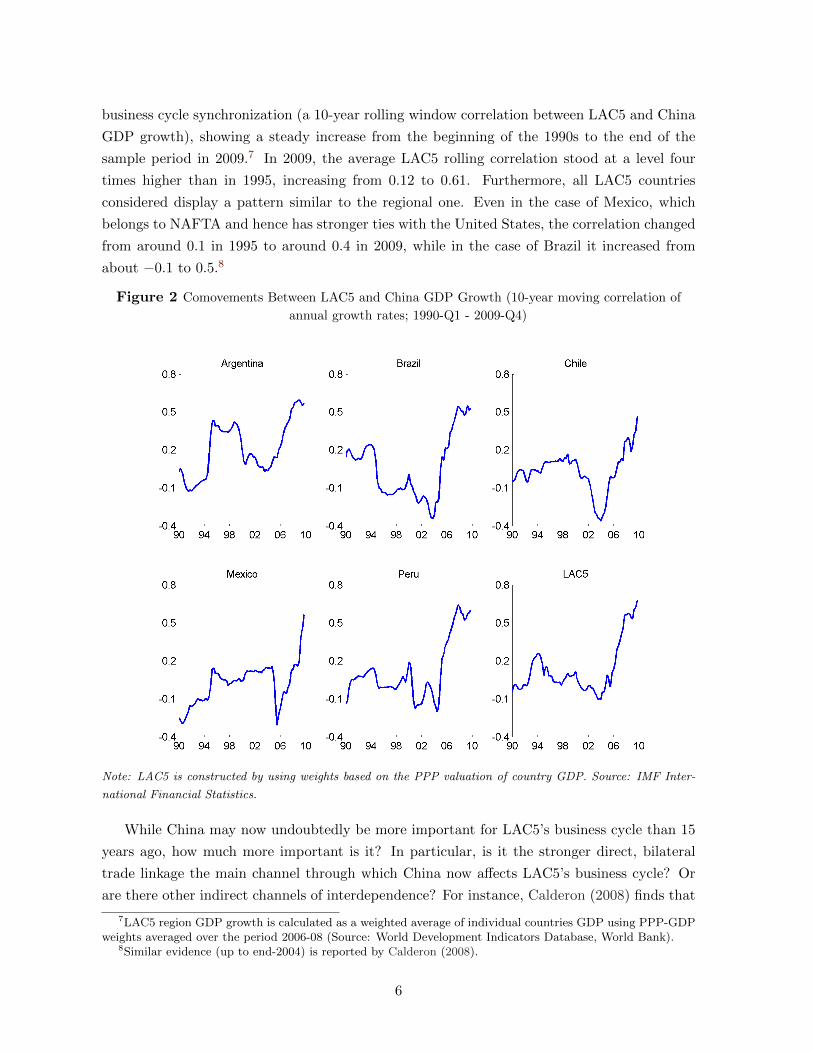
business cycle synchronization (a 10-year rolling window correlation between LAC5 and China

GDP growth), showing a steady increase from the beginning of the 1990s to the end of the

sample period in 2009.7 In 2009, the average LAC5 rolling correlation stood at a level four

times higher than in 1995, increasing from 0.12 to 0.61. Furthermore, all LAC5 countries

considered display a pattern similar to the regional one. Even in the case of Mexico, which

belongs to NAFTA and hence has stronger ties with the United States, the correlation changed

from around 0.1 in 1995 to around 0.4 in 2009, while in the case of Brazil it increased from

about −0.1 to 0.5.8

Figure 2 Comovements Between LAC5 and China GDP Growth (10-year moving correlation of

annual growth rates; 1990-Q1 - 2009-Q4)

Note: LAC5 is constructed by using weights based on the PPP valuation of country GDP. Source: IMF Inter-

national Financial Statistics.

While China may now undoubtedly be more important for LAC5’s business cycle than 15

years ago, how much more important is it? In particular, is it the stronger direct, bilateral

trade linkage the main channel through which China now affects LAC5’s business cycle? Or

are there other indirect channels of interdependence? For instance, Calderon (2008) finds that

7LAC5 region GDP growth is calculated as a weighted average of individual countries GDP using PPP-GDPweights averaged over the period 2006-08 (Source: World Development Indicators Database, World Bank).

8Similar evidence (up to end-2004) is reported by Calderon (2008).

6

China affects LAC5’s business cycle mostly via its demand for commodities. And the decade-

long commodity price boom might be inflating the bilateral trade shares between China and

LAC5 plotted in Figure 1. In addition, there are also other indirect channels of influence related

to international capital flows and China’s exchange rate regime that might play a role.9

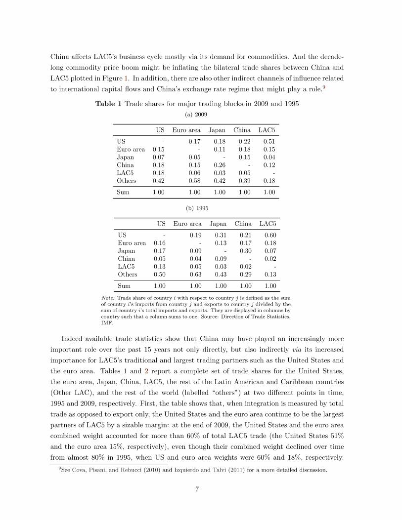
Table 1 Trade shares for major trading blocks in 2009 and 1995

(a) 2009

US Euro area Japan China LAC5

US - 0.17 0.18 0.22 0.51Euro area 0.15 - 0.11 0.18 0.15Japan 0.07 0.05 - 0.15 0.04China 0.18 0.15 0.26 - 0.12LAC5 0.18 0.06 0.03 0.05 -Others 0.42 0.58 0.42 0.39 0.18

Sum 1.00 1.00 1.00 1.00 1.00

(b) 1995

US Euro area Japan China LAC5

US - 0.19 0.31 0.21 0.60Euro area 0.16 - 0.13 0.17 0.18Japan 0.17 0.09 - 0.30 0.07China 0.05 0.04 0.09 - 0.02LAC5 0.13 0.05 0.03 0.02 -Others 0.50 0.63 0.43 0.29 0.13

Sum 1.00 1.00 1.00 1.00 1.00

Note: Trade share of country i with respect to country j is defined as the sumof country i’s imports from country j and exports to country j divided by thesum of country i’s total imports and exports. They are displayed in columns bycountry such that a column sums to one. Source: Direction of Trade Statistics,IMF.

Indeed available trade statistics show that China may have played an increasingly more

important role over the past 15 years not only directly, but also indirectly via its increased

importance for LAC5’s traditional and largest trading partners such as the United States and

the euro area. Tables 1 and 2 report a complete set of trade shares for the United States,

the euro area, Japan, China, LAC5, the rest of the Latin American and Caribbean countries

(Other LAC), and the rest of the world (labelled “others”) at two different points in time,

1995 and 2009, respectively. First, the table shows that, when integration is measured by total

trade as opposed to export only, the United States and the euro area continue to be the largest

partners of LAC5 by a sizable margin: at the end of 2009, the United States and the euro area

combined weight accounted for more than 60% of total LAC5 trade (the United States 51%

and the euro area 15%, respectively), even though their combined weight declined over time

from almost 80% in 1995, when US and euro area weights were 60% and 18%, respectively.

9See Cova, Pisani, and Rebucci (2010) and Izquierdo and Talvi (2011) for a more detailed discussion.

7

Table 2 Trade shares for LAC5 countries in 2009 and 1995

(a) 2009

Argentina Brazil Chile Mexico Peru

US 0.12 0.17 0.20 0.70 0.25Euro area 0.17 0.23 0.16 0.07 0.14

Japan 0.02 0.05 0.08 0.02 0.06China 0.13 0.16 0.18 0.06 0.16

Other LAC 0.43 0.17 0.20 0.03 0.20Others 0.13 0.21 0.18 0.12 0.18

Sum 1.00 1.00 1.00 1.00 1.00

(b) 1995

Argentina Brazil Chile Mexico Peru

US 0.16 0.25 0.23 0.83 0.29Euro Area 0.26 0.28 0.21 0.06 0.22Japan 0.03 0.08 0.14 0.03 0.08China 0.03 0.03 0.02 0.00 0.05Other LAC 0.39 0.18 0.20 0.02 0.19Others 0.13 0.18 0.19 0.06 0.18

Sum 1.00 1.00 1.00 1.00 1.00

Note: Trade weights are computed as shares of exports and imports. Theyare displayed in columns by country such that a column sums to one. Source:Direction of Trade Statistics, IMF.

In contrast, China’s share of LAC5’s total trade surged in all LAC5 countries except Mexico

(only moderate increase) over the same period mostly at the expense of the United States and

the euro area (see Table 2 ), but remains much smaller than the United States and the euro

area. Second, the table shows that China’s emergence as a global trade power has also affected

LAC5’s largest trade partners: China’s share in total trade of the United States, the euro area,

and Japan grew to 18%, 15%, and 26% in 2009, from 5%, 4%, and 9% in 1995, respectively.

This stylized evidence suggests that China today might be affecting LAC5’s business cycle

not only via its stronger direct trade linkages, but also through its stronger indirect linkages

with LAC5’s main traditional trade partners. In the rest of the paper we shall quantify how

these changes in the geographical composition of trade have affected the transmission of specific

shocks to LAC5 and the rest of the world economy, and also attempt, to the extent possible,

to disentangle direct effects via stronger bilateral link boosted by commodity price increases,

and the indirect effects via larger influences on traditional trading partners.10

10Other indirect transmission channels, such as financial linkages, are taken into account in the GVAR modelthrough the inclusion financial variables, but are not discussed separately in the paper, because comparablecounter-factual simulation exercises to those used to investigate trade linkages cannot be constructed, due tothe limited availability of reliable data on bilateral financial positions.

8

3 The GVAR Methodology

In this section we present the GVAR methodology, discuss some of its underlying assump-

tions, the nature of the counterfactual experiments conducted, and the type of shocks to be

considered.

The GVAR modelling strategy consists of two main steps. First, each country is modeled

individually as a small open economy by estimating a country-specific vector error-correction

model in which domestic variables are related to country-specific foreign variables and global

variables that are common across all countries (such as the price of oil). The foreign variables

provide the link between the evolution of the domestic economy and the rest of the world and,

in estimating the country-specific models, are taken as (weakly) exogenous—an assumption

that is tested in the paper. Second, a global model is constructed combining all the estimated

country-specific models and linking them with a matrix of predetermined (i.e., not estimated)

cross-country linkages. We now present and discuss each of these two steps in turn.11

3.1 The first step: specification and estimation of country-specific models

Consider N + 1 countries in the global economy, indexed by i = 0, 1, 2, ...N . In the first step,

with the exception of country “0” (that in our application is the United States), all other

N countries are modelled as small open economies in which a set of domestic variables (xit,

to be specified below) is related to a set of country-specific foreign variables, x∗it, using an

augmented vector autoregressive model (VARX*) specification. Specifically, for each country

i, we set up a VARX*(pi,qi) model in which the ki×1 vector, xit, is related to the k∗i ×1 vector

of country-specific foreign variables, x∗it, and the md × 1 global variables, dt, plus a constant

and a deterministic time trend:

Φi(L, pi)xit = ai0 + ai1t+ Υi(L, qi)dt + Λi(L, qi)x∗it + uit, (3.1)

with t = 1, 2, ..., T . Here Φi(L, pi) = I −∑pi

i=1 ΦiLi is the matrix lag polynomial of the

coefficients associated with xit; ai0 is a ki × 1 vector of fixed intercepts; ai1 is the ki × 1

vector of coefficients on the deterministic time trends; Υi(L, qi) =∑qi

i=0 ΥiLi is the matrix

lag polynomial of the coefficients associated with dt; Λi(L, qi) =∑qi

i=0 ΛiLi is the matrix lag

polynomial of the coefficients associated with x∗it; uit is a ki × 1 vector of country-specific

shocks, which we assume serially uncorrelated, with zero mean and a nonsingular covariance

matrix, Σii, namely uit ∼ i.i.d.(0,Σii).12

The vector of country-specific foreign variables, x∗it, plays a central role in the GVAR

11See Dees, di Mauro, Pesaran, and Smith (2007) and Garratt, Lee, Pesaran, and Shin (2006) for a detailedillustration of the GVAR methodology.

12Notice that we allow Φi(L, pi), Υi(L, qi), and Λi(L, qi) to differ across countries. The lag orders, pi and qi,are also selected on a country by country basis.

9

methodology. Consistent with the existing GVAR literature, for each country i at each time t,

this vector is constructed as the weighted average across all countries j of the corresponding

variables in the model (xjt for j 6= i). As a way of dealing with the curse of dimensionality

when N is relatively large, the weights used in the construction of x∗it are not estimated but

specified a priori, based on information that measures the strength of bilateral linkages in the

global economy. While the GVAR methodology can be implemented with any set of weights,

the existing GVAR literature, as well as the application in this paper, use trade weights.

Specifically, the weight of country j in the foreign variables of country i is given by the share

of country j in the total trade of country i (as described in footnote no. 6).

The choice of trade weights is based on a number of considerations. First, trade in goods

represents an important (if not the most important) channel through which shocks are trans-

mitted across countries. Second, trade linkages tend to reflect deeper technological, political

and cultural linkages that exist between countries and provide a good measurable proxy for

such inter-connections. Third, amongst the alternative measures that could be used, trade

weights are perhaps the most reliable, and data sources are readily available to quantify them.

Reliable bilateral trade statistics are published annually for all countries (with a few excep-

tions), while data on bilateral financial flows are either non existent or tend to be much more

volatile and less reliable as their collection has started only more recently. The use of bilateral

financial flows could therefore exaggerate the cross country transmission of shocks and lead to

parameter instability. Finally, we note that trade integration started much earlier than finan-

cial integration and has been present throughout our sample period. China, the main focus

of this paper, is an example of a country whose expansion has affected the rest of the world

dramatically and yet its financial system is not internationally connected—the same applies to

other emerging market economies in our model.

It is also worth highlighting that, in the case of a GVAR model, comprising small open

economies, the choice of weights is of secondary importance for the estimation of country-

specific parameters, particularly since the variables tend to be highly correlated across coun-

tries. In fact, as shown by Pesaran (2006), for sufficiently large N , the estimation results are

asymptotically invariant to the choice of weights so long as they are “granular”, namely of

order 1/N . However, as the application in this paper shows, the impulse response of shocks

to a particular variable in the GVAR does depend on the choice of weights even if similar pa-

rameter estimates are obtained using different sets of weights. This is a particularly important

consideration for the present paper where the focus of the analysis is on the possible effects of

changing trade linkages between LAC5 and the world economy.

With this in mind, we develop a GVAR model where trade weights are allowed to change at

the estimation stage as well as at the solution stage (when impulse responses are computed), in

contrast to most other applications of the GVAR to date that are based on fixed trade weights.

This methodological innovation is important as it allows us to take into account the evidence

10

that trade integration has progressed over time and the geographical patterns of trade have

changed dramatically with the acceleration of globalization in the mid-1990s as we documented

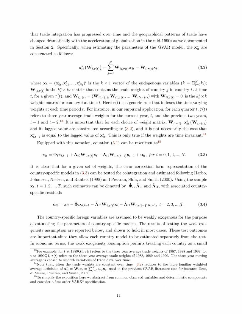
in Section 2. Specifically, when estimating the parameters of the GVAR model, the x∗it are

constructed as follows:

x∗it(Wi,τ(t)

)=

N∑j=0

Wij,τ(t)xjt = Wi,τ(t)xt, (3.2)

where xt = (x′0t,x′1t, ...,x

′Nt)′ is the k × 1 vector of the endogenous variables (k = ΣN

i=0ki);

Wij,τ(t) is the k∗i × kj matrix that contains the trade weights of country j in country i at time

t, for a given τ(t); and Wi,τ(t) = (Wi0,τ(t),Wi1,τ(t), ...,WiN,τ(t)) with Wii,τ(t) = 0 is the k∗i ×kweights matrix for country i at time t. Here τ(t) is a generic rule that indexes the time-varying

weights at each time period t. For instance, in our empirical application, for each quarter t, τ(t)

refers to three year average trade weights for the current year, t, and the previous two years,

t − 1 and t − 2.13 It is important that for each choice of weight matrix, Wi,τ(t), x∗it(Wi,τ(t)

)and its lagged value are constructed according to (3.2), and it is not necessarily the case that

x∗i,t−1 is equal to the lagged value of x∗it. This is only true if the weights are time invariant.14

Equipped with this notation, equation (3.1) can be rewritten as15

xit = Φixi,t−1 + Λi0Wi,τ(t)xt + Λi1Wi,τ(t−1)xt−1 + uit, for i = 0, 1, 2, ..., N. (3.3)

It is clear that for a given set of weights, the error correction form representation of the

country-specific models in (3.3) can be tested for cointegration and estimated following Harbo,

Johansen, Nielsen, and Rahbek (1998) and Pesaran, Shin, and Smith (2000). Using the sample

xt, t = 1, 2, ..., T , such estimates can be denoted by Φi, Λi0 and Λi1, with associated country-

specific residuals

uit = xit − Φixi,t−1 − Λi0Wi,τ(t)xt − Λi1Wi,τ(t−1)xt−1, t = 2, 3, ..., T. (3.4)

The country-specific foreign variables are assumed to be weakly exogenous for the purpose

of estimating the parameters of country-specific models. The results of testing the weak exo-

geneity assumption are reported below, and shown to hold in most cases. These test outcomes

are important since they allow each country model to be estimated separately from the rest.

In economic terms, the weak exogeneity assumption permits treating each country as a small

13For example, for t at 1989Q4, τ(t) refers to the three year average trade weights of 1987, 1988 and 1989; fort at 1990Q1, τ(t) refers to the three year average trade weights of 1988, 1989 and 1990. The three-year movingaverage is chosen to smooth variations of trade data over time.

14Note that, when the trade weights are constant over time, (3.2) reduces to the more familiar weightedaverage definition of x∗it = Wixt =

∑Nj=0 ωijxjt used in the previous GVAR literature (see for instance Dees,

di Mauro, Pesaran, and Smith, 2007).15To simplify the exposition here we abstract from common observed variables and deterministic components

and consider a first order VARX* specification.

11

open economy with respect to the rest of the world. Also note that the number of countries

does not need to be large to build a GVAR model. Nonetheless, when the number of countries

is relatively small, the weak exogeneity assumption may not be satisfied for all countries. It is

only when the number of countries is relatively large (technically, tending to infinity), and all

countries are comparable in size, that we can have a fully symmetric treatment of all the mod-

els in the GVAR. For this reason, as we shall see below, we treat the United States differently

as a dominant economy, consistent with previous applications of GVAR.

3.2 The second step: building the GVAR

In the second step, the GVAR model is set up by stacking the estimated individual country-

specific models and linking them with a matrix of predetermined cross-country linkages. Hav-

ing estimated the country-specific parameters using the time varying weights, the estimated

country-specific models can now be combined and solved for any given trade weights based

on a particular year, or on an average of weights from different time periods. In what follows,

denote such a link weight matrix by W0i , with i = 0, 1, ...N , and define the ki × k selection

matrix Si such that

xit = Sixt. (3.5)

Then rewrite equation (3.3) in terms of xt = (x′0t,x′1t, ...,x

′Nt)′, which contains all the endoge-

nous variables in the global model:

Sixt = ΦiSixt−1 + Λi0W0i xt + Λi1W

0i xt−1 + uit,

or

Gixt = Hixt−1 + uit, (3.6)

where

Gi = Si − Λi0W0i , (3.7)

Hi = ΦiSi + Λi1W0i . (3.8)

Now stacking (3.6) for i = 0, 1, ..., N we have

Gxt = Hxt−1 + ut, (3.9)

where

G = (G′0,G′1, ...,G

′N )′, and H = (H′0,H

′1, ...,H

′N )′.

Finally, assuming then that G is non-singular we obtain

xt = Fxt−1 + G−1ut, (3.10)

12

where F = G−1H. The GVAR model in (3.10) can then be used to compare impulse responses

for any set of link matrices W0i , i = 0, 1, ...N .16 But several remarks are in order.

First, given that we are interested in the impact of changing trade patterns on the trans-

mission of shocks of global relevance, we propose to solve the GVAR (estimated in the first

step) for weights or link matrices at different points in time. Thus, in the empirical section

of the paper, we consider the implications of the same estimated country-specific models but

for different choices of trade weights. Note that the GVAR model parameters are estimated

only in the first stage and are taken as given in the second stage. Under the assumption that

these parameters are stable over time, the global model can be safely used counterfactually

with alternative trade matrices as we do in our application.

Second, each alternative trade matrix represents a particular counterfactual of interest that

leads to a different set of residuals. In fact, uit defined by (3.6) is not the same as uit in (3.4),

unless the weights used in the first stage at each time t are the same as in the second stage,

namely if Wi,τ(t−1) = W0i , for all t. This condition can only occur when the weights used in

the first stage are fixed and match the weights used in the second stage, which is not the case

in our application. Thus, in general, the uit’s might be contemporaneously as well as serially

correlated, even if the residuals of the fitted model in (3.4) are not.

To quantify the uncertainty around the GIRF point estimates, we use a non-parametric

bootstrap procedure, which requires an estimate of the covariance matrix of the stacked

country-specific residuals ut = (u′0t, u′1t, ..., u

′Nt)′, Σu. One possible estimate is the sample

moment matrix,

Σu =

∑T−1t=2 utu

′t

(T − 1).

Notice, however, that in our application where the dimension of the endogenous variables in

the GVAR model (k) is larger than the time series dimension (T ), Σu is not guaranteed to be

a positive definite matrix. This is an important consideration when computing bootstrapped

error bands for the impulse responses or bootstrapped critical values for the structural stability

tests. To avoid this problem, following Dees, Pesaran, Smith, and Smith (2010) we use a

shrinkage estimator of the covariance matrix in the empirical analysis, as explained in Appendix

B.

Third, interdependence among countries in the GVAR model arises through many different

channels. Direct trade linkages are only one of the important channels. The different country

variables are also connected through the dependence of xit on global variables dt, and through

the contemporaneous interdependence of shocks in country i on shocks in country j, as summa-

rized by the estimated cross-country covariances, Σij , where Σij = Cov(uit,ujt) = E(uitu′jt)

for i 6= j. It is also worth noting that, unless we link the country specific models in a coherent

16See appendix B.1 for more detailed discussion and derivation of the solution to the GVAR with a givenweight matrix.

13

manner, as in the second step of the modeling strategy explained above, impulse responses of

shocks to domestic and foreign variables can not take account of the second and higher order

interaction in the global system. For this reason, as we shall see below, altering the direct

trade linkages between county i and j by altering the respective coefficient in the link matrix

above does not necessarily change the bilateral interdependence between the two countries.

Finally, the shocks we consider in the paper are not identified, unlike what is claimed

in the structural VAR literature.17 We focus instead on shocks that could be triggered by

different fundamental sources of disturbances, such as productivity, monetary policy, or other

structural shocks, without attempting to identify the ultimate source of the disturbance. To

distinguish between the different factors that contribute to a particular variable change, it

often involves incredible identifying assumptions. For instance, researchers are still debating

about the identification of a US technology shock in a closed economy model. Moving to a

global model, such issues become even more vexing, and in this paper we do not try to identify

the effects of a US (or China technology shock for that matter) from all the other sources of

disturbances that could prevail in the global economy.18

To investigate the transmission of shocks to the country-specific variables, we use gener-

alized impulse response functions (GIRFs). GIRFs, developed in Koop, Pesaran, and Potter

(1996) and Pesaran and Shin (1998), take into account the possibility that the error terms

of the GVAR are contemporaneously correlated across variables and countries. For instance,

a country-specific GDP shock can ultimately be stemming from a shift in demand or supply

of output in that country, in other countries, or globally. GIRFs for such a shock show how

changes in a given variable (say US GDP), or a linear combination of changes in a number of

variables (say global output), affect the other variables in the GVAR on impact (first round

effects) and over time (second and higher order effects) regardless of the source of the change.

As noted above, GIRFs do not answer the “deeper” question of whether such changes originate

from technology shock, monetary policy shocks, oil shocks, or other structural shocks. Instead,

they describe what happens if there are changes to the errors, uit, of the conditional model,

(3.1), without trying to identify the sources of such changes. Unlike the errors in the standard

VAR models, the shocks in the conditional models that comprise the GVAR are only weakly

cross sectionally correlated, which lend further support to the use of GIRFs for the analysis of

the transmission of shocks across countries. The evidence on cross country correlation of the

errors of the country-specific VARX* model is given in Section C.5.2.

17In principle, traditional impulse responses to orthogonalized shocks could also be computed, but they woulddepend on the specific identification scheme adopted. For instance, in the case of the typically used Choleskyscheme, the results would depend on the ordering of the variables and/or countries in the model, while GIRFsare invariant to such orderings.

18See Dees, Pesaran, Smith, and Smith (2010) for an attempt to do so in a GVAR version of the canonical(three-equation) New Keynesian model.

14

4 A GVAR Model for Latin America in the World Economy

In this section we discuss the model specification and report test results to check the validity

of the weak exogeneity assumption of country-specific foreign variables and the stability of the

parameters.

4.1 Model specification

The GVAR model that we specify includes 26 country-specific VARX* models, as displayed

in Table 3. We consider all major advanced and emerging economies in the world accounting

for about 90% of world GDP, including five Latin American economies (Argentina, Brazil,

Chile, Peru, and Mexico)19 and a euro area block. The euro area block is made up of its

8 largest economies: Germany, France, Italy, Spain, Netherlands, Belgium, Austria and Fin-

land.20 Thus, the version of the GVAR model that we specify uses data for 33 countries. The

models are estimated over the period 1979Q2-2009Q4, thus including both the great recession

of 2008 and 2009 and the first two quarters of the recent global recovery.

Table 3 Countries and Regions in the GVAR Code

Core economies Euro Area Latin AmericaUS Austria ArgentinaChina Belgium BrazilUK Finland ChileJapan France Mexico

Germany PeruOther developed countries ItalyAustralia NetherlandsCanada SpainNew Zealand

Rest of Emerging Asia Rest of Western Europe Rest of the worldIndonesia Norway IndiaKorea Sweden South AfricaMalaysia Switzerland Saudi ArabiaPhilippines TurkeySingaporeThailand

With the exception of the US model, all country models include the same set of variables,

where available (see Table 4). The variables included in each country model are real GDP

(yit), the rate of inflation (πit = pit − pi,t−1), the real exchange rate defined as (eit − pit),

19Data availability is the only constraint to the number of Latin American countries included.20The time series data for the euro area are constructed as weighted averages using Purchasing Power Parity

GDP weights, averaged over the 2006-2008 period (Source: World Bank). A more detailed description of datais reported in the Appendix A.

15

and, when available, real equity prices (qit), a short rate (ρSit) and a long rate of interest

(ρLit), with: yit = ln(GDPit/CPIit), pit = ln(CPIit), qit = ln(EQit/CPIit), eit = ln(Eit),

ρSit = 0.25 · ln(1 + RSit/100), ρLit = 0.25 · ln(1 + RLit/100), where GDPit is nominal Gross

Domestic Product of country i at time t (in domestic currency); CPIit is the Consumer Price

Index in country i at time t (equal to 100 in year 2000); EQit is a nominal Equity Price Index;

Eit is the nominal exchange rate of country i at time t in terms of US dollars; RSit is the short

rate of interest in percent per year (typically a three-month rate); RLit is a long rate of interest

in percent per year (typically a ten year rate). All country models (except the US) also include

the log of nominal oil prices (pot ) as a weakly exogenous foreign variable.

The US model is specified differently. First, oil price is included as an endogenous variable.

In addition, given the importance of the US financial variables in the global economy, the

US-specific foreign financial variables, q∗US,t, and ρ∗LUS,t, are not included in the US model (see

below for a discussion on the results of the weak exogeneity test applied to these variables).

Note also that the real value of the US dollar, by construction, is determined outside the US

model, and the US-specific real exchange rate (defined as e∗US,t − p∗US,t) is included in the US

model as a weakly exogenous foreign variable.

Table 4 Variables Specification of the Country-specific VARX* Models

Non-US models US model

Domestic Foreign Domestic Foreign

yit y∗it yUS y∗US

πit π∗it πUS π∗

US

qit q∗it qUS

ρSit ρS∗it ρSUS ρS∗

US

ρLit ρL∗it ρLUS -

eit − pit - - e∗US − p∗US

- pot pot -

Note: In the non-US models the inclusion of the listed vari-

ables depends on data availability.

4.2 Country-specific estimates and tests

Given the importance of the weak exogeneity assumption in the construction of the GVAR

model, and the parameter stability for the counterfactual simulation exercise that we conduct

in the paper, we focus on the evidence on these two sets of test statistics in our discussion.21

21Due to space considerations, detailed empirical evidence on the statistical assumptions made to specify theGVAR model is reported in Appendix C, together with a description of the impact multipliers and averagepair-wise correlations for all variables and countries included in the model. We also report evidence on unit roottests, lag order selection, and the cointegration rank for all country models in Appendix C.

16

As noted above, for all countries, we treat the foreign variables as weakly exogenous. To

test for the weak exogeneity of country-specific foreign variables and oil prices, the individual

country models are first estimated under the null hypothesis that foreign variables are indeed

weakly exogenous. The resultant error correction terms are then included in the auxiliary

equations for country specific foreign variables, and their statistical significance are tested

jointly. Under the null hypothesis that foreign variables are weakly exogenous, the error

correction terms must not be statistically significant.22

We find that the weak exogeneity hypothesis could not be rejected for the majority of vari-

ables considered, especially for core economies such as the US, euro area and China. Specifi-

cally, only 10 out of the 156 exogeneity tests performed result in rejection of the weak exogeneity

hypothesis. Not surprisingly, given the relative size and role of Latin America in the world

economy, almost all foreign variables in the LAC5 models can be treated as weakly exogenous.

Only foreign output in the model for Mexico and oil prices in the model for Brazil cannot

be considered as weakly exogenous according to the test statistics reported. But such results

can also arise by chance: given that we use a 5 percent significance level, we would expect

at least 5 percent of the 130 tests performed to fail (i.e., 6 or 7) even if the weak exogeneity

hypothesis were valid in all cases. Note that China meets the weak exogeneity assumption

despite its greatly increased importance in the world economy. Indeed, while it is possible that

with China continuing its current rate of expansion at some point in the future it ceases to

become “small”, our test results suggest that at present China can still be viewed as a small

open economy for the purpose of estimating the model parameters. As we shall see, however,

this does not mean that its increased weight in the world economy does not matter when we

come to analyze the transmission of shocks emanating from its economy.

For the United States, the null hypothesis of weak exogeneity can be rejected for US-

specific foreign equity prices at 5% level, due the prominence of US equity markets in the

global context. The weak exogeneity of US-specific foreign long run interest rates, however,

can not be rejected at 5% level. Given the size and importance of US equity and bond markets

in international financial markets, we decided to exclude foreign long run interest rates and

foreign equity prices from the US model. The foreign counterpart of output, inflation and real

exchange rate (defined above) pass the weak exogeneity test and are therefore included in the

US model. Note that, differently from the specification estimated by Dees, di Mauro, Pesaran,

and Smith (2007), the US-specific foreign short term interest rate, ρ∗SUS,t, also passes the weak

exogeneity test and is included as a weakly exogenous variable in the US model.

The possibility of structural breaks is of particular concern in the case of emerging countries,

which have been subject to significant political, social and structural changes during our sample

period. Note, however, that the GVAR implicitly accommodates co-breaking (Mizon and

22The details of the testing procedure and the results for the weak exogeneity test are presented in AppendixC (see Table C.6 for results).

17

Hendry, 1998), implying that the VARX* models that make up the GVAR are more robust to

the possibility of structural breaks as compared to standard VAR models or single equation

models. Focusing on Latin American real GDP variables, in particular, structural breaks

are found in years when these countries were subject to severe shocks that coincide with the

starting and ending of the hyperinflation periods in Brazil and Peru. While acknowledging

that this evidence is problematic, we follow earlier GVAR work (see, for example, Pesaran,

Schuermann, and Weiner, 2004 and Dees, di Mauro, Pesaran, and Smith, 2007) and provide

bootstrap means and confidence bounds for the point estimates, that do allow for breaks in

the error variance-covariances.23

5 Transmission of Shocks Before and After China’s Rise in the

World Economy

To quantify the change in the transmission of external shocks to Latin America before and after

the acceleration of the globalization process at the beginning of the 1990s, and the emergence of

China as a significant trading nation, we conduct a set of counter-factual simulation exercises

along the lines discussed in Section 3. That is, while keeping constant the parameters of the

VARX* models estimated in the first step of the GVAR methodology (with foreign variables

constructed using time-varying trade weights), we solve the GVAR model in the second step

with four different sets of trade matrices, based on fixed trade weights for the years 1985, 1995,

2005, and 2009. We then compare the resultant time profiles of the transmission of specific

GDP shocks across different counter-factual trade linkages.

By focusing on this four sets of trade weights we can quantify how changed geographical

trade patterns may have altered the impact and transmission of shocks to LAC5 and the world

economy, abstracting from any implied changes to parameter estimates that might have taken

place as a result of changing trade weights. As we saw in Section 2, trade weights were relatively

stable over the period 1985-1995, while they started to change steadily after 1995. Therefore,

we expect the most marked changes to be associated with weights in years 1995 and 2009.

Trade weights in years 1985 and 2005 are also considered because they give a better sense of

the time-evolution of the estimated impacts and provide some evidence on the robustness of

the results.

Our GVAR model has 134 variables (all endogenously determined), and there are numer-

ous potentially relevant shocks that could be considered.24 We consider two country-specific

shocks with potential global impacts, namely a China GDP shock and a US GDP shock, and

investigate how their effects on the GDP of selected countries in the GVAR model (including

23See Appendix C.4 for a detailed account of parameter stability tests.24A full set of GIRFs for the baseline model is not reported but is available from the authors upon request. In

Appendix C, we report a full set of impact multipliers that represent one summary dimension of the internationallinkages in the GVAR.

18

particularly LAC5 economies) change using alternative trade matrices. In addition to a China

GDP shock that is the main focus of our application, we look at a shock to US GDP because

it provides a natural benchmark against which to contrast the results for China. We focus

on GDP shocks because they are of particular interest in light of the recent global crisis. We

also consider a LAC5 GDP shock and a GDP shock to the rest of emerging Asia (excluding

India) because they shed light on the ongoing debate on the “decoupling” of emerging markets’

business cycles from that of advanced economies. In the analysis of the international trans-

mission of these shocks we look at both regional and country-specific responses. The regional

responses are constructed as weighted averages of the country specific responses, using weights

based on the PPP valuation of country GDP, which provide good measures of relative sizes of

the economies under consideration.

As we noted earlier, unlike Dees, Pesaran, Smith, and Smith (2010), we do not attempt to

interpret these GDP shocks structurally, for instance, distinguishing between demand and sup-

ply sources of output change in the analysis. Note however that in the GVAR model, once xit is

conditioned on x∗it, the estimated country specific shocks have effectively little or no correlation

across countries.25 Thus, country specific GDP shocks, conditional on the rest of the world

GDP variables (that are present in every country model considered), albeit not orthogonal,

have little or no cross-country correlations. This makes it possible to consider GIRFs to US

or China GDP shocks with little concerns about reverse spillover effects from one country to

the other. Nonetheless, we find that contemporaneous correlation of the shocks within country

models remains sizable even after conditioning on global variables thus precluding a structural

interpretation of these country GDP shocks as supply or demand shocks, for example, without

further a priori restrictions.

With these preliminary considerations in mind, the rest of this section reports and discusses

the results of the counterfactual simulations that we have carried out. We report the point

estimates of the GIRFs in the main text in Figures 3 to 7, while the bootstrap error band

results are reported in Figures C.2 to C.9 in Appendix C.

5.1 A China GDP shock

Figure 3 presents the GIRFs for a one percent increase in China GDP, using 2009, 2005, 1995

and 1985 trade weights. In the LAC5 region as a whole, the long-run response to this shock

with 2009 weights is almost three times as large as the one associated with 1995 weights. The

responses of all individual LAC5 countries are qualitatively similar, but there are quantitative

differences across countries in the region. The long-run responses of Chile and Brazil increase

the most (almost four times); whilst those of Mexico and Peru increase the least. Interestingly,

however, even the changes in the short run response of Mexico GDP are sizable (reaching almost

25See Tables C.10 and C.11 in Appendix C for detailed account of the average pairwise correlations of errorsin the country-specific models of the GVAR.

19

Figure 3 GIRFs for One Percent Increase in China GDP(World economy and LAC5; point estimates; 1985, 1995, 2005, and 2009)

0.3 percent as with the other LAC5 countries in 2009), despite the much larger importance of

NAFTA trade in Mexico’s total trade. This is because, as we shall see below, a China GDP

shock affects both the United States and Canada in a much stronger way with 2009 weights,

and thus also Mexico, albeit indirectly rather than directly. In contrast, it is puzzling that the

20

strength of the impact and the transmission of the shock does not increase in the case of a

commodity exporter like Peru, despite the fact that its trade shares have evolved in a manner

similar to other LAC5 countries (see Figure 1).

With more recent trade weights (2005 and 2009 weights), a China GDP shock matters

much more for both advanced and other emerging economies, in particular in the long run.

For instance, the long run impact of the shock on the United States with 2009 weights has

increased by about 50 percent compared to 1995 weights and by about 100 percent since 1985.

For the euro area and Canada, the changes in the transmission of a China GDP shock are even

more marked than in the case of the United State with 2005 and 2009 weights. While in the

case of Japan the increase in the impact is less pronounced, the rest of emerging Asia exhibits

the same pattern of progressively increasing responses to a China GDP shock when using more

recent weights that the rest of the world displays. Only India, whose trade integration with

the rest of the world is mainly driven by trade in services (not accounted for in the available

trade statistics that we use to compute trade linkages), seems to be affected relatively less by

a China GDP shock with more recent trade weights. Moreover, differences between 2009 and

1985 responses to a China GDP shock are not only quantitatively sizable but also statistically

significant in the sense that, in most cases, the 95 percent error bands for the bootstrapped

2009 responses do not contain zero values. In contrast, the effects are not statistically different

from zero if we consider the 1985 trade weights.26

The reported changes in the transmission of the China GDP shock to LAC5 and the rest

of the world economy are likely to have played an important role in the unfolding of the recent

global financial and economic crisis. For instance, Cova, Pisani, and Rebucci (2010) estimate

that, absent the large fiscal stimulus enacted by China during the global crisis, China’s GDP

would be 2.6 percentage points lower in 2009. The estimated elasticities to a China GDP

change reported in Figure 3 imply that US GDP growth would have been a quarter percentage

point lower, and LAC5 GDP growth would have been almost a full percentage point lower in

2009.27 Conversely, suppose that China growth slowed in the medium to long term to about 7

percent per annum, as for instance currently forecasted in China’s 12th official five-year plan.

This would shave almost a half percentage point from LAC5 long-term growth–probably more

than 10 percent of the region’s growth potential– with much larger short term effects.28 These

26See Figures C.2 and C.3 in Appendix C for the bootstrapped impulse responses. Note that the pointestimates do not need to coincide with the mean of the bootstrapped distribution. The point estimates arebased on a one percent shock to GDP, while the bootstrapped distributions are based on a one standarddeviation shock to GDP.

27With 2009 trade weights, the peak impacts of a China GDP shock on US GDP and LAC5 GDP are 0.12percent and 0.3 percent, respectively.

28We conduct the following calculations: if China’s growth rate falls by 3 percentage points to 7 percentper year, given the long run elasticity of a China GDP shock on LAC5 GDP is estimated to be about 0.15, itimplies a fall in LAC5 GDP growth of around 0.4-0.5 percentage points in the long run. Assuming that thelong run growth rate of LAC5 is between 4 and 5 percent per year (say for example, as in the case of Brazil), areduction of GDP growth by 0.4-0.5 percentage points represents a decline in potential growth of approximately10 percent.

21

Figure 4 GIRFs for One Percent Increase in China GDP: Total and Indirect Effect(World economy and LAC5; point estimates; 2009, Indirect 2009, and 1995)

Note: The indirect effect (labeled “Indirect 2009”) is computed by lowering the trade shares of China in the

LAC5 countries (except Mexico) to their 1995 levels.

are quite sizable effects, especially considering that these back of the envelop calculations do

not account for any likely associated financial market over-reaction to such important changes

in the fundamental driver of the region’s business cycle.

In light of Mexico’s responses to a China GDP shock, and more generally the stylized

facts discussed in Section 2, it is interesting to see whether the increased impact of a China

GDP shock on other LAC5 countries is due to the stronger direct or indirect trade linkages.

That is, it would be interesting to quantify whether the stronger impact of China on LAC5 is

more due to stronger bilateral trade ties between China and LAC5, or to a stronger indirect

effects emanating from the impact of China on LAC5’s traditional and largest trade partners,

namely, the United States and the euro area. To separate out these two effects we conduct an

additional counterfactual simulation. In this experiment, we take the 2009 trade matrix and

change the weights of China in total trade of LAC5 economies with the exception of Mexico

to 1995 levels (thus resetting the direct trade links between the region and China to the 1995

level). All other entries in the link matrix are initially kept at their 2009 values (thus leaving

the indirect links via United States and the euro area unchanged). The difference between

22

the 1995 and the 2009 weight of China in the total trade of each of the four LAC countries is

then redistributed proportionally to the remaining countries excluding the United States and

the euro area, which are left unchanged at their 2009 levels. Note that, in this experiment, we

also leave Mexico’s direct trade link with China unchanged at its 2009 level. This is because,

otherwise, the response of the United States to the China GDP shock with this “hybrid” link

matrix would change due to Mexico’s large trade share in US total trade, and the exercise

would overstate the effects on Mexico.29

The results are reported in Figure 4 and show that the indirect linkages are likely to be more

important than the direct linkages; thus highlighting the strength of the general equilibrium

dynamics that the GVAR modelling strategy captures. As we can see, muting the change in

the direct trade link between China and LAC5 (excluding Mexico) has no consequences on

the United States, the euro area, and Mexico itself by construction. This is because LAC5

excluding Mexico (whose trade shares are kept constant) is too small in trade terms to affect

the United States. In the case of Brazil, Chile and Argentina, the changes in the impact of the

China GDP shock due to changed indirect linkages are at least as large as those due to changes

in the direct links: changed indirect linkages in fact explain at least half of the total change in

the transmission of the shock, and almost all of the change in the case of Brazil. In the case of

Peru, there is a very small total change, and hence the distinction is immaterial. We interpret

this evidence as suggesting that both direct and indirect effects contribute to the stronger

impact of China GDP shock on LAC5 countries, but the indirect channel of transmission is

at least as important as the more obvious direct links. In some cases, like Brazil, the indirect

effects seem to be even more important than the direct effects.

This is clear evidence that, as we shall see more formally below, the changed trade linkages

between China, Latin America and the rest of the world are affecting the region not only via

stronger direct trade linkages (boosted by a persistent increase in commodity prices that inflate

the trade shares of LAC), but also via stronger ties between China and LAC5’s traditional

trading partners. An important implication of this result is that other countries in the broader

LAC region, such as countries in Central America and the Caribbean, might now be more

affected by China via increased impact of China GDP shock on the United States and the euro

area. This result also suggests that the increased impact of a China GDP shock on Mexico

discussed above can be interpreted as a result of stronger indirect trade linkages between China

and the other NAFTA member countries.

5.2 A US GDP shock

Figure 5 presents the GIRFs for a one percent increase in US GDP. The impact of a US GDP

shock on advanced and emerging market economies falls considerably with more recent trade

29In fact, Mexico has a 14 percent share of total trade of the United States in 2009, based on the IMF Directionof Trade Statistics.

23

Figure 5 GIRFs for One Percent Increase in US GDP(World economy and LAC5; point estimates; 1985, 1995, 2005, and 2009)

weights, especially in the short term, mirroring the shift in the geographical distribution of

trade discussed in Section 2. Specifically, the impact of the shock on the United States itself

with 2009 weights is almost half its size with 1995 weights in the first few quarters, and is

about 20-25 percent weaker over the longer term. The results for Canada are similar. In the

24

case of the euro area the transmission of the shock weakens more uniformly across the horizon

of the GIRF. The bootstrapped impulse responses to this shock suggest that these differences

are not only quantitatively sizable, but also statistically significant (Figures C.4 and C.5 in

Appendix C).

In the case of LAC5, the short term impact of this shock falls dramatically (becoming

statistically insignificant) with 2009 weights, while the long run impact halves as compared to

the one with 1995 weights. Like in the case of the China GDP shock, there are quantitative

differences in responses of individual LAC5 countries, but the qualitative pattern is common

across all the five countries. The long run responses of Chile decrease the most, by almost a

half compared with 1995 trade weights. In comparison to LAC5 average, perhaps not surpris-

ingly the reduction in the responses of Mexico is the smallest but still sizable, given Mexico’s

membership of NAFTA.

The changes in the impact of the US GDP shock on Asia are more mixed. The long

run impact on China GDP falls dramatically with 2009 weights compared with the estimates

corresponding to the 1985 weights. However, these differences are significant only for the first

two quarters. Japan and the rest of emerging Asia (driven by Korea that is not reported

separately) show some differences in the short run effects, but the evidence does not imply

a reduction in the impact of a US GDP shock on these economies in the long run. And the

bootstrapped responses show that these changes are not statistically significant.

These results imply that the effect of the recent US “great recession” on LAC5 would have

been much more severe if this event had taken place in the mid-1990s. For instance, Izquierdo

and Talvi (2011) estimate that the level of US GDP at the peak of the recession was more than

7 percent below its potential. If the crisis had taken place in the mid-1990s rather than at the

end of the 2000s, our simulations show that LAC5 could have experienced the same output gap

as the United States based on these estimates.30 It is evident that while good initial conditions

at the beginning of the crisis and prompt international financial support have helped the LAC5

region to cope well with the recent global crisis, less dependency on the country in the epicenter

of the crisis (the United States) has proven to be fortunate for the economic performance of

the region during the crisis.

5.3 A GDP shock in Latin America and the Rest of Emerging Asia

Consider now a one percent increase in LAC5 GDP, and in the GDP of emerging Asia excluding

China and India. Figures 6 and 7 display the point estimates of the GIRFs for these two regions.

These shocks are constructed as the weighted average (PPP-GDP average) of shocks to GDP

in all LAC5 and emerging Asian countries in the model, respectively.31 As it can be seen, the

30The long run impact of a 1% rise in US GDP shock on LAC5 output is about 1% with 1995 weights, butonly about 0.4% with 2009 weights.

31The list of countries in the “Rest of Emerging Asia” group is in Table 3.

25

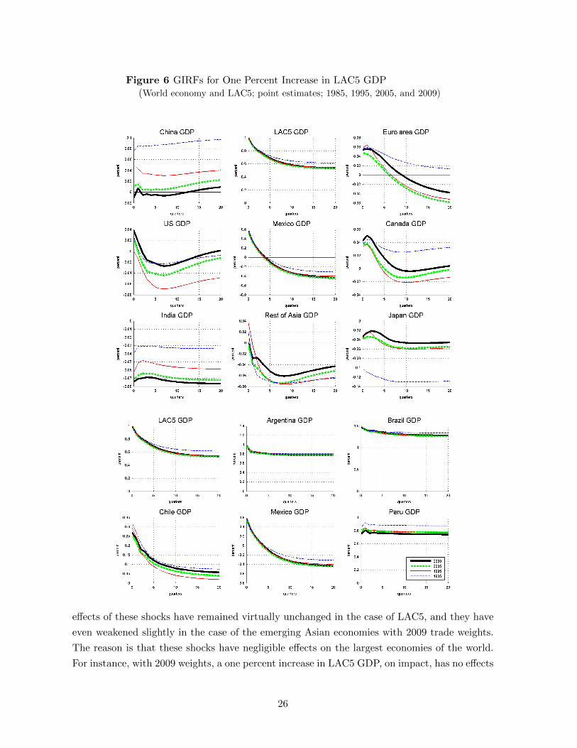
Figure 6 GIRFs for One Percent Increase in LAC5 GDP(World economy and LAC5; point estimates; 1985, 1995, 2005, and 2009)

effects of these shocks have remained virtually unchanged in the case of LAC5, and they have

even weakened slightly in the case of the emerging Asian economies with 2009 trade weights.

The reason is that these shocks have negligible effects on the largest economies of the world.

For instance, with 2009 weights, a one percent increase in LAC5 GDP, on impact, has no effects

26

Figure 7 GIRFs for One Percent Increase in rest of Asia GDP(World economy and LAC5; point estimates; 1985, 1995, 2005, and 2009)

on China and Japan GDP, and its effects on the euro area GDP is equal to half of the impact

of a China GDP shock discussed before. The LAC5 shock has an impact on US GDP that

is similar to that of a China GDP shock, but the impact of the LAC5 shock (mostly through

Mexico) dies out in two quarters, while the shock to China GDP has a hump-shaped response,

27

peaking above 0.1 percent within three to four quarters.

The bootstrapped GIRFs confirm that the transmission of these shocks to the rest of the

world economy is not statistically significant with 2009 trade weights.32 In contrast, we can

see that while a LAC5 GDP shock has a widespread, if short lived, impact on the rest of the

world economy with 1985 weights, this impact becomes insignificant with 2009 weights. In

the case of a GDP shock to emerging Asia, the transmission to the rest of the world is not

statistically significant even with 1985 weights.

These results speak to an extent to the much-debated “decoupling” hypothesis. According

to this hypothesis (see Kose and Prasad, 2010 for instance), emerging markets have “decoupled”

from advanced economies in recent years in the sense that their growth dynamics has become

more autonomous. As a result, emerging markets as a group are starting to be a autonomous

source of world growth. The results above, taken together with those on the transmission of a

China GDP shock, show that LAC5 and the rest of emerging Asia (excluding China and India)

are still too small to have a meaningful impact on the world economy. They cannot, therefore,

be counted as an autonomous source of world growth, like China; at least as yet.

What our findings also suggest is that LAC5 and the rest of emerging Asia remain a collec-

tion of small open economies whose fluctuations can be affected strongly by the international

business cycle. The key change we document is that their cycle is now more exposed to China

and less exposed to the US compared to the past (although the impact of a US GDP shock

remains sizable). And not only directly via stronger bilateral trade ties, but also, and perhaps

more importantly, via China’s stronger ties with advanced economies. In other words, the evi-

dence reported in this paper suggests that the “decoupling” of emerging market from advanced

economies found in the existing literature (e.g., Kose and Prasad, 2010) is more likely related

to the emergence of China as an important source of world growth as opposed to a widespread

“decoupling” of emerging markets business cycle from that of advanced economies.

6 Conclusions

In this paper we investigated how China’s emergence in the world economy has affected the

international transmission of business cycles to 5 large Latin American economies. Using a

GVAR model for the 26 largest advanced and emerging economies in the world, estimated with

quarterly data from 1979Q2 to 2009Q4 with time-varying trade weights, we conducted a series

of counterfactual exercises with different sets of trade weights for years 1985, 1995, 2005, and

2009.

We found that the long-run impact of a China GDP shock on the typical Latin American

economy has increased three times since the mid-1990s. In contrast, and consistent with the

32See Figures C.6 to C.9 for the bootstrapped impulse responses to a LAC5 GDP shock and a GDP shock toemerging Asia.

28

previous findings, the long run effect of a US GDP shock has halved over the same period, with

even sharper declines in the short term impact. We show that the larger impacts of a China

GDP shock owe as much to indirect effects, associated with stronger trade linkages between

China and Latin America’s largest trade partners–the United States and the euro area–as to

direct effects stemming from tighter trade linkages between China and Latin America, boosted

by the decade-long boom in commodity prices that has inflated trade shares. The results also

suggest that the transmission of domestic shocks originating in Latin America and the rest of

emerging Asia (excluding China and India) has not changed much over the same period.

These findings help to explain why the five Latin American economies we consider recovered

much faster than initially anticipated from the recent global crisis. In fact the evidence shows

that Latin America growth now owes more to a fast-growing economy that enacted a powerful

fiscal stimulus during the global crisis and relatively less to the economy that was at the

epicenter of the crisis. Had the trade linkages been those prevailing in the mid-1990s, the

region would have likely suffered a much sharper downturn than it actually experienced. This

evidence also suggests that the “decoupling” found in the existing literature might be related

to the emergence of China as an important source of world growth as opposed to a more general

tendency of emerging markets’ business cycles to decouple from that of advanced economies.

But the same findings expose new vulnerabilities for Latin America and the rest of the world

economy. Latin America remains a small open economy vulnerable to external shocks, without

the necessary weight to affect the international business cycle with its own growth dynamics.

Latin America, and the rest of the world economy, including its traditional and still largest

trading partners, now relies relatively more on China and less on the United States compared

to only 15 years ago. China is a large, low-middle income economy whose transition to high

income economy will continue for many years to come. But China is also a relatively less stable

and more volatile economy than the United States.33 While the changes documented have had

positive, stabilizing effects on Latin America business cycle during the recent global crisis, the

same facts may predict negative, and destabilizing effects if and when China’s growth begins

to slow down. Thus, going forward, Latin America and the rest of the world economy are likely

to become more volatile places.

33In fact, the average conditional standard deviation of a China GDP shock in the first stage of the GVARanalysis is more than twice as large that of the United States.

29

A Data Appendix: Data Source & Data treatment

A.1 Data sources

This version of the GVAR dataset revises and extends up to 2009Q4 the dataset used inPesaran, Schuermann, and Smith (2009b) (PSS hereinafter) which covers the period 1979Q1-2006Q4. Data were collected in June 2010 and we refer to the updated dataset as the “2009Vintage”.34

A.1.1 Real GDP

In order to compile the 2009 Vintage Real GDP, we used the International Financial Statistics(IFS) database and Inter-American Development Bank Latin Macro Watch Database (IDBLMW hereinafter).35 Countries are divided into three groups. First, those for which quarterlyand seasonally adjusted data are available. Second, those for which quarterly data are available,but they are not seasonally adjusted. Third, those for which only annual data are available.

For the first group, we used the IFS 99BVRZF series (GDP VOL) for Australia, Canada,France, Germany, Italy, Japan, Netherlands, New Zealand, South Africa, Spain, Switzerland,United Kingdom, and United States. We extrapolated the PSS data set using quarterly growthrates of the IFS series from 2004Q1 to 2009Q4.

For the second group, we used the IFS 99BVPZF series (GDP VOL) for Austria, Bel-gium, Finland, India, Indonesia, Korea, Malaysia, Norway, Singapore, Sweden, Thailand, andTurkey. These series were seasonally adjusted using Eviews, applying the National Bureau’sX12 program.36 As in the first group, the dataset was extended with forward extrapolation ofPSS data, using quarterly growth rates of the adjusted IFS series from 2004Q1 to 2009Q4.

For Saudi Arabia the annual seasonally unadjusted IFS BVPZF GDP VOL series wasinterpolated to obtain the quarterly values.37 This series was then treated as the quarterlyseasonally unadjusted data. For Philippines, the quarterly rate of change of a seasonal adjustedreal GDP index (Source: Bloomberg. Ticker: PHNAGDPS Index) was used to extrapolateforward PSS data from 2004Q1 to 2009Q4.

For Latin American countries, namely for Argentina, Brazil, Chile, Mexico, and Peru, theIDB LMW data was used (Series: GDP, Real Index s.a.) and the series were updated in thesame manner as described for quarterly seasonally adjusted data.

In PSS Chinese quarterly GDP was interpolated from IFS annual data, as for Saudi Arabia.Given the increasing importance of China in the world economy, the construction of a quarterlyreal GDP index from national sources may provide some value added. As no institutionpublishes a quarterly real GDP Index for China, it has to be compiled from a nominal GDPseries. The National Bureau of Statistics (NBS) of China releases quarterly nominal GDP serieswithout seasonal adjustments.38 Accordingly, we constructed a quarterly real GDP index for

34The Pesaran, Schuermann, and Smith (2009b) dataset is, in turn, an extension of the dataset used inPesaran, Schuermann, and Smith (2009a) which covers the period 1979Q1-2005Q4.

35For further information see http://www.iadb.org/Research/LatinMacroWatch/lmw.cfm36Seasonal adjustment was performed on the log difference of GDP using the additive option. Then, using

the first observation of the un-adjusted log GDP series, we accumulate the adjusted log-changes. Finally, weobtained seasonally adjusted level series by taking the exponential of the log adjusted series.

37The interpolation procedure is described in Supplement A of Dees, di Mauro, Pesaran, and Smith (2007).38The NBS series can be assessed from Datastream, ticker: CH GDP (DS CALCULATED) CURN.

30

China as follows. First, we seasonally adjusted (with the procedure described below in SectionA.2) the nominal GDP from NBS. Then, we used the following formula

log(RGDP1) = log(GDP1CPI1

)for t = 1

log(RGDPt) = log(RGDPt−1) + log(

GDPtGDPt−1

)− log

(CPItCPIt−1

)for t ≥ 2

where CPI is defined in Section A.1.2. The series display noisy features in the first part of thesample and starts to show more plausible patterns from 1994Q1 onwards, providing a naturalcut-off date. Therefore, we used the new series from 1994Q1 to 2009Q4 and we extrapolatedbackward to 1979Q1 using the quarterly rate of change of the China GDP series in PSS.39

A.1.2 Consumer price index

In order to create the 2009 Vintage CPI, IFS CPI 64zf (level) series were collected for allcountries with the exception of China. For countries which do not need seasonal adjustment,the quarterly growth rates of these series were used to extrapolate forward the PSS datafrom 2001Q1 to 2009Q4. Consistently with the procedure in Section A.2.1, the CPI series forthe following countries were seasonally adjusted: Austria, Belgium, Canada, Chile, Finland,France, Germany, India, Italy, Japan, Korea, Mexico, Netherlands, New Zealand, South Africa,Spain, Sweden, Switzerland, Thailand, United Kingdom, and United States.40 The quarterlyrate of change of the adjusted IFS series was used to extrapolate forward PSS data from 2000Q1to 2009Q4, in order to obtain the 2009 CPI Vintage.

For China, Datastream data (Source: National Bureau of Statistics. Ticker: CHCONPR%F.YoY rate of change, NSA) was used. The Datastream rate of change was used to create a seriesin level which was then seasonally adjusted using Eviews, applying the National Bureau’s X12program.41 The 2009 Vintage CPI for China was obtained by forward extrapolation of PSSdata set using the rate of change of the adjusted Datastream series from 2000Q1 to 2009Q4.

A.1.3 Equity price index

Updated equity price series are from Bloomberg, whilst the PSS data set uses Datastream. Wetook a quarterly average of the MSCI Country Index in local currency for each of the followingcountries: Argentina, Australia, Austria, Belgium, Canada, Chile, Finland, France, Germany,India, Italy, Japan, Korea, Netherlands, Norway, New Zealand, Philippines, South Africa,Spain, Sweden, Switzerland, Thailand, United Kingdom, and United States.42 For Malaysia,as the MSCI Index is not available, we took a quarterly average of the local composite indexfrom Datastream (Ticker: KLPCOMP. Local currency). The quarterly average was computedbased on close price of the last Wednesday of each month. That is, we used the last Wednesday

39Notice that the China GDP series is subject to major data revisions. For this reason, we updated thenominal China GDP series in April 2011 (after the most recent data revision) and used the updated series toconstruct our real GDP measure.

40Seasonal adjustment was performed with Eviews, using X12 program with the additive option. See alsoSection A.2 below.

41We used the same procedure here as for real GDP.42To construct a MSCI Country Index, every listed security in the market is identified. Securities are free

float adjusted, classified in accordance with the Global Industry Classification Standard (GICS), and screenedby size, liquidity and minimum free float (Source: MSCI Barra, www.mscibarra.com).

31

for each month, then we took a simple average of these Wednesday prices for the first threemonths of the year to obtain our first quarterly price index. Then we took average of theWednesday values for the next three months to get the second quarterly price index and so on.Finally, the 2009 Vintage Equity Price Index was obtained by forward extrapolation of PSSdata using the rate of change of the new series from 2004Q1 to 2009Q4.

A.1.4 Exchange rates

Exchange rates series are from Bloomberg. We took a quarterly average of the nominal bilat-eral exchange rates vis-a-vis the US dollar (units of foreign currency per US dollar) for eachcountry.43 The quarterly average was computed based on close value of the last Wednesdayof each month, as described for Equity Price Index. The 2009 Vintage Exchange Rate wasobtained by forward extrapolation of the PSS data set using the rate of change of the newseries from 2004Q1 to 2009Q4.

Notice that the exchange rate series of the euro economies refer to the pre-euro exchangerate (i.e. national currency per dollar). To denominate them in euro, we took the quarterlyaverage of the euro exchange rate vis-a-vis the US dollar (Source: Bloomberg. Ticker: EURCurncy). We then used the 1999Q1 value of this series as the base and extrapolate it backwardand forward using the rate of change of the series denominated in national currencies.

A.1.5 Short term interest rates

IFS is the main source of data for short term interest rates. Consistently with PSS, the IFSDeposit Rate (60Lzf series) is used for Argentina, Chile, China, and Turkey. The IFS DiscountRate (60zf series) is used for New Zealand and Peru. The IFS Treasury Bill Rate (60Czfseries) is used for Canada, Malaysia, Mexico, Philippines, South Africa, Sweden, UK and US.The IFS Money Market Rate (60Bzf series) is used for Australia, Brazil, Finland, Germany,Indonesia, Italy, Japan, Korea, Norway, Singapore, Spain, Switzerland, and Thailand. ForAustria, Belgium, France, and the Netherlands no data is available for any of these seriesfrom 1999Q1 when the euro was introduced. We used the country specific IFS Money MarketRate (60Bzf series) from 1979Q1 to 1998Q4 and completed the series to 2009Q4 using thecorresponding data (60Bzf series) for Germany as the representative euro area interest rate.

For India, quarterly averages of daily Bloomberg data (India Treasury Bill 3-Month Yield44.Ticker: GINTB3MO Index) are constructed in the same way as the quarterly exchange rateseries. When IFS data was not available, gaps were filled using Bloomberg data: Norway in2007Q1 and 2009Q4 (Ticker: NKDRC CMPN Curncy), Philippines from 2008Q4 to 2009Q1(Ticker: PH91AVG Index), Sweden from 2009Q2 to 2009Q4 (Ticker: GSGT3M Index). ThePSS data series are extended with these series from 2004Q1 to 2009Q4.

43The list of Bloomberg tickers is as follows: ARS JPMQ Curncy, AUD BGN Curncy, ATS CMPN Curncy,BEF CMPN Curncy, BRL BGN Curncy, CAD BGN Curncy, CNY BGN Curncy, CLP BGN Curncy, COPBGN Curncy, FIM CMPN Curncy, FRF CMPN Curncy, DEM BGN Curncy, INR CMPN Curncy, IDR BGNCurncy, ITL BGN Curncy, JPY BGN Curncy, KRW BGN Curncy, MYR BGN Curncy, MXN BGN Curncy,NLG CMPN Curncy, NOK BGN Curncy, NZD BGN Curncy, PEN BGN Curncy, PHP BGN Curncy, ZAR BGNCurncy, SAR BGN Curncy, SGD BGN Curncy, ESP CMPN Curncy, SEK BGN Curncy, CHF BGN Curncy,THB BGN Curncy, TRY BGN Curncy, GBP BGN Curncy, VEF BGN Curncy.

44This is an indicative Treasury Bill Rate polled daily by Bloomberg from various sources. The constructedseries is not exactly equal to the original DdPS series, however they are very close (Corr: 99.63%).

32

A.1.6 Long term interest rates

The IFS Government Bond Yield (61zf series) is used to extend data for all 18 countries forwhich long term interest rate data is available, namely Australia, Austria, Belgium, Canada,France, Germany, Italy, Japan, Korea, Netherlands, New Zealand, Norway, South Africa,Spain, Sweden, Switzerland, United Kingdom, and United States. The PSS data series areextended with these series from 2004Q1 to 2009Q4.

A.1.7 Oil price index

For the Oil Price we used a Brent crude oil price from Bloomberg (Series: Current pipelineexport quality Brent blend. Ticker: CO1 Comdty). To construct the quarterly series, we tookaverage of daily close prices for all trading days within the quarter. The quarterly rate ofchange of this new series was used to extrapolate forward the PSS data set from 2004Q1 to2009Q4.

A.1.8 PPP-GDP weights

The main source for the country specific GDP weights is the World Development Indicatordatabase of the World Bank. The GDP in Purchasing Power Parity terms in current interna-tional dollars (Ticker: NY.GDP.MKTP.PP.CD) was downloaded for all countries from 2006 to2008.

A.1.9 Trade matrices

To construct the trade matrices, we use the IMF Direction of Trade statistics. For all thecountries considered we downloaded the matrix of Exports and Imports (c.i.f.) with annualfrequency. The data for 2009 Exports and Imports is appended to the original PSS dataset.We use trade matrices for 1979–2009 for estimation in our paper.

A.2 Seasonality

A.2.1 Assessing the joint significance of seasonal effects

To assess the joint significance of the seasonal components for real output and inflation serieswe used the following procedure:

1. Let S1; S2; S3 and S4 be the usual seasonal dummies, such that Si, i = 1, 2, 3, 4, takesthe value of 1 in the ith quarter and zero in the other three quarters.

2. Construct S14 = S1− S4, S24 = S2− S4, S34 = S3− S4.

3. Run a regression of ∆y (where the lower case stands for the natural logarithm of thecorresponding variable) on an intercept and S14; S24; S34: Denote the OLS estimatesof S14; S24 and S34 by a1; a2 and a3.

4. Asses the joint significance of the seasonal components by testing the null hypothesisthat a1 = a2 = a3 = 0 using the F-statistic.

33

5. In cases where the null hypothesis is rejected at the 10% level, seasonal adjustmentwas performed on the log-difference of the original series using the X-12 procedure asdescribed below.

A.2.2 Method of seasonality adjustment

To seasonally adjust log(GDP ) series (assumed to be an I(1) process), we first seasonally adjust∆log(GDP ) using the X-12 quarterly seasonal adjustment method in Eviews with the additiveoption, to obtain ∆ log(GDP )SA. Then use the first observation of raw series log(GDP ) (levels,not seasonally adjusted) and the seasonally adjusted series of the changes, ∆ log(GDP )SA, toobtain the seasonally adjusted level series log(GDP )SA.

Consider now the updating of seasonally adjusted series, and suppose we have seasonallyadjusted series from 1979Q1 to 2006Q4, and we wish to update the series to 2009Q4. Wedownload the raw series, for example from 2000Q1 to 2009Q4, and seasonally adjust with theprocedure described above. We then use the seasonally adjusted new series in growth rates, toupdate the original seasonally adjusted series. To avoid possible abrupt changes in the updatedseries, we also overwrite two years of the original series for all variables except for inflation. Inthe case of inflation we overwrite six years of original series due to major data revisions in theinflation series. Specifically, we update all series (except inflation) from 2004Q1 to 2009Q4,and inflation series from 2000Q1 to 2009Q4.

B Technical Appendix. GVAR Solution and Bootstrapping

B.1 Solution of the GVAR with a given weight matrix

We present detailed derivation of the solution of the GVAR with a given weight matrix in thisappendix, and show that the estimated country specific models (from the first step) can bestacked and solved for any given trade weights, which we denote by W0

i . Let’s also denoteWNT to be the set of all weight matrices, which we use to estimate the country specific modelsin the first step,

WNT = {Wit, i = 0, 1, ..., N ; t = 1, 2, ..., T} .

Then, the country-specific estimates of the VARX* in equation (3.4) can be denoted byΦi(WNT ), Λi0(WNT ), and Λi1(WNT ) and the associated residuals by uit(WNT ). Also,let θi(WNT ) = (V ec(Φi(WNT ))′, V ec(Λi0(WNT ))′, V ec(Λi1(WNT ))′)′, and use the ki × kselection matrix Si such that

xit = Sixt.

Then

Sixt = Φi(WNT )Sixt−1 + Λi0(WNT )W0i xt + Λi1(WNT )W0

i xt−1 + uit,[Si − Λi0(WNT )W0

i

]xt =

[Φi(WNT )Si + Λi1(WNT )W0

i

]xt−1 + uit

Gi(θi(WNT ))xt = Hi(θi(WNT ))xt−1 + uit, (B.1)

34

where

Gi(θi(WNT ),W0i ) = Si − Λi0(WNT )W0

i (B.2)

Hi(θi(WNT ),W0i ) = Φi(WNT )Si + Λi1(WNT )W0

i (B.3)

Note that uit will NOT be the same as uit(WNT ), unless at time t we have Wi,τ(t−1) = W0i ,

which can only occur when the weights are fixed. Stacking (B.1) for i = 0, 1, ..., N we have

G(θ(WNT ),W0

)xt = H

(θ(WNT ),W0

)xt−1 + ut,

where

G(θ(WNT ),W0

)= (G′0(θ0(WNT ),W0

0),G′1(θ1(WNT ,W01)), ...,G′N (θN (WNT ,W

0N )))′,

H(θ(WNT ),W0

)= (H′0(θ0(WNT ),W0

0),H′1(θ1(WNT ),W01), ...,H′N (θN (WNT ,W

0N ))))′,

θ(WNT ) = (θ′0(WNT ), θ′1(WNT ), ..., θ′N (WNT ))′, and W0= (W00,W

01, ...,W

0N ).

Therefore,

xt = F(θ(WNT ),W0

)xt−1 + G−1

(θ(WNT ),W0

)ut, (B.4)

whereF(θ(WNT ),W0

)= G−1

(θ(WNT ),W0

)H(θ(WNT ),W0

). (B.5)

If we abstract from parameter uncertainty and take the value of θ(WNT ) as given and “true”,then n-step ahead forecasts are given by

E (xt+n |It−1 ) =[F(θ(WNT ),W0

)]n+1xt−1.

Similarly, the n-step ahead generalized impulse response of the effect of a unit shock to ξt = a′uton the composite variable qt = b′xt , where a and b are k × 1 selection vectors, is given by

gq(n, σξ) =b′[F(θ(WNT ),W0

)]nG−1

(θ(WNT ),W0

)Σua

√a′Σua

. (B.6)

σξ =√

a′Σua is the size of the unit shock to ξt. The error covariance matrix can be estimatedusing the residuals uit defined by (B.1). One possible estimate is the sample moment matrix,

Σu = (T −1)−1T−1∑t=2

utu′t, where ut = (u′0t, u

′1t, ..., u

′Nt)′. One could also use a shrinkage version

of Σu. Since N is large relative to T we use a shrinkage estimator of Σu defined by

Σu(λ) = λΣu + (1− λ)Diag(Σu), (B.7)

where λ is the shrinkage parameter andDiag(Σu) is a diagonal matrix formed from the diagonalelements of Σu.

35

B.2 Bootstrapping the GVAR model with time varying weights

To derive the empirical distribution of the structural stability tests and of the impulse responsefunctions we use a non-parametric bootstrap procedure. The non-parametric bootstrap proce-dure aims at taking account of the sampling uncertainty associated with the estimates θ(WNT ),for given values of WNT and W0. In this case the appropriate residuals for the purpose ofdrawing bootstrapped samples are uit, given by (B.1). This suggests generating the bootstrap

samples, denoted by x(b)t , b = 1, ..., B, according to the process

x(b)t = F

(θ(WNT ),W0

)x

(b)t−1 + G−1

(θ(WNT ),W0

)u

(b)t (B.8)

for t = 1, 2, ..., T , where F(θ(WNT ),W0

)is given by (B.4), x

(b)0 = x0, (x

(b)−1 = x−1 if a

GVAR(2) is considered), and where x0 and x−1 are the realized initial data vectors. For each

b, u(b)t is generated by random draws from ut allowing for the fact that Σu is non-diagonal

and can be singular. This can be achieved using the Cholesky factor of Σu (or a shrinkageversion of it) along the lines proposed in the supplement to Dees, di Mauro, Pesaran, andSmith (2007).

To carry out the Cholesky factorization the estimated error variance covariance matrix mustbe non-singular, and we also use a shrinkage parameter defined by (B.7). In the applicationsreported in the paper Σu(λ) becomes non-singular for values of λ ≥ 0.8, but to reduce theeffects of the sampling errors in the Cholesky factorization of Σu(λ) we decided to set λ = 0.5,half way between the sample estimate and its diagonal version. For consistency between thepoint estimates and bootstrapped results, we also set λ = 0.5 for the point estimates. Finally,prior to any resampling, the residuals were recentered to ensure that their bootstrap populationmean is zero.

For each bootstrap sample, b, the individual country models must be estimated with thesame set of time varying weights, WNT , lag orders and cointegrating rank. Denote the param-eter estimates based on the bth bootstrap sample by θ(b)(WNT ). Then the associated impulseresponse functions across the different bootstrapped replications are given by

g(b)q (h, σξ) =

b′[F(θ(b)(WNT ),W0

)]hG−1

(θ(b)(WNT ),W0

)Σ

(b)u a√

a′Σ(b)u a

, (B.9)

for b = 1, 2, ..., B. The bootstrap confidence bounds can now be computed for each h using

the percentiles of g(b)q (h, σξ), over b = 1, 2, ..., B.

C Appendix: Additional Estimation Results and BootstrappedGIRFs

In this section we present and discuss formal specification tests for key aspects of the model,namely, integration properties of the series, lag-length selection and cointegration rank, weakexogeneity of foreign variables, and parameter stability. In addition, we comment on some ofthe main estimation results such as impact elasticities, and pairwise cross-section correlationof variables and residuals. Finally, we present bootstrapped GIRFs, to complement the results

36

on the point estimates in the main body of the paper.

C.1 Unit root tests

The GVAR model can be specified in terms of either stationary or integrated variables.Nonetheless, here we follow Dees, di Mauro, Pesaran, and Smith (2007) and we assume thatthe variables included in the country-specific models are integrated of order one (or I(1)). Thispermits us to distinguish between short run and long run relations and interpret the long runrelations as cointegrating.

To examine the integration properties of both the domestic and foreign variables we useunit root tests. Given the recognized poor performance of ADF tests in small samples, weconsider unit root t-statistics based on weighted symmetric estimation of ADF type regressionsintroduced by Park and Fuller (1995) (WS hereafter).45 The lag length employed in the WSunit root tests is selected by the Akaike Information Criterion (AIC) based on standard ADFregressions.

Results of the WS statistics for the level, first differences and second differences of thecountry-specific domestic and foreign variables are reported in Tables C.2 and C.3. Thisbattery of tests generally support the unit root hypothesis, with only a few exceptions. First,the null hypothesis of unit root for Mexico GDP is rejected by the test. Nonetheless, thisis a boarder line case and if we look at a more standard ADF test, we do not reject theunit root hypothesis. Second, the unit root hypothesis for long-term interest rates in mostadvanced economies and for the real exchange rate in Mexico and UK is also rejected. Forthe UK, Switzerland, China and some other developing countries, the unit root hypothesisfor inflation is rejected. On inflation, since overdifferencing is likely to be less serious of aspecification error than wrongly including an I(2) variable, we opt for the inclusion of inflationas an I(1) variable, as in Pesaran, Schuermann, and Weiner (2004). In fact, the order ofintegration of a variable is not in general a property of an economic variable but a convenientstatistical approximation to distinguish between the short-run, medium-run, and long-runvariations in the data. With the adoption of a medium-run perspective, which is consistentwith nonstationarity of most of economic variables, treating inflation as a stationary variable islikely to invalidate the statistical analysis. For the remaining countries and variables, the testresults generally support our working assumption that the variables included in the country-specific models can be treated as I(1) variables.

C.2 Selecting lag orders and cointegration ranks

We select lag orders and cointegaration ranks of the country-specific cointegrating VARX*models under the assumptions that the included foreign variables are weakly exogeneous, andthat the parameters of the individual models are stable over time. Evidence for these hypothe-ses will be discussed in the next two sub-sections.

45Dees, di Mauro, Pesaran, and Smith (2007) argue that the weighted symmetric ADF tests exploit the timereversibility of stationary autoregressive processes in order to increase their power performance. Leybourne, Kim,and Newbold (2005) and Pantula, Gonzalez-Farias, and Fuller (1994) provide evidence of superior performanceof the weighted symmetric ADF test in comparison to the standard ADF test of the GLS-ADF test proposedby Elliott, Rothenberg, and Stock (1996). See also Chapter 4 of Microfit 5 Manual (Pesaran and Pesaran, 2009)for a detailed discussion.

37

Table C.1 Lag Orders of the Country-specific VARX*(pi,qi) Models and the Number ofCointegrating Relations

pi qi CV pi qi CVChina 1 1 1 Malaysia 1 1 1Euro area 2 1 1 Philippines 2 1 1Japan 2 1 1 Singapore 1 1 1Argentina 1 1 1 Thailand 2 1 1Brazil 1 1 1 India 1 1 1Chile 1 1 2 S. Africa 2 1 1Mexico 1 1 2 S. Arabia 2 1 1Peru 1 1 1 Turkey 2 1 2Australia 1 1 2 Norway 1 1 2Canada 2 1 1 Sweden 1 1 1N. Zealand 1 1 2 Switzerland 2 1 2Indonesia 1 1 1 UK 2 1 1Korea 2 1 1 US 2 1 2

We select the lag orders, pi and qi, of the individual country VARX*(pi,qi) models ac-cording to the Akaike information criterion under the constraints imposed by data limitations.Accordingly, the lag order of the foreign variables, qi, is set equal to one in all countries; for thesame reason, we constraint pi ≤ 2. Notice that, since we observed in preliminary analysis ofthe GIRFs very ragged responses for Argentina, Brazil, Chile, Peru, New Zealand, Indonesia,India, Norway and Sweden, we changed the orders of the VARX* models for these countriesfrom VARX*(2, 1) to VARX*(1, 1).

We then proceed with the cointegration analysis, where the country specific models are esti-mated subject to reduced rank restrictions (Johansen, 1992). To this end, the error-correctionforms of individual country equations are derived. The rank of the cointegrating space for eachcountry was tested using Johansen’s trace and maximal eigenvalue statistics as set out in Pe-saran, Shin, and Smith (2000) for models with weakly exogenous I(1) regressors, unrestrictedintercepts and restricted trend coefficients.

The order of the VARX* models as well as the number of cointegration relationships arepresented in Table C.1. Tables C.4 and C.5 report the trace test statistics and the 95% criticalvalues for all the country-specific VARX* models, respectively. The critical values are takenfrom MacKinnon (1991). We chose the trace test, because it has better small sample propertiescompared to the maximal eigenvalue test.

To address the issue of possible overestimation of the number of cointegration relationshipsbased on asymptotic critical values, and to assure the stability of the global model, we re-duced the number of cointegration relations for a number of countries (see, for example, Dees,di Mauro, Pesaran, and Smith, 2007). Specifically, the following adjustments in the numberof cointegration relations have been made from the results implied by the statistical tests:Argentina from 3 to 1, Peru from 3 to 1, Chile from 3 to 2, Mexico from 3 to 2, Australiafrom 4 to 2, Canada from 3 to 1, New Zealand from 3 to 2, Japan from 3 to 1, Korea from 5to 1, Singapore from 3 to 1, Thailand from 2 to 1, Saudi Arabia from 2 to 1, Indonesia from2 to 1, South Africa 2 from to 1, Philippines from 2 to 1, India from 2 to 1, euro area from2 to 1, and UK from 3 to 1. These shrinkage in the number of cointegration relations provednecessary for arriving at convergent persistent profiles for the various cointegration relations.The persistence profiles refer to the time profiles of the effects of system or variable specific

38

shocks on the cointegration relations in the GVAR model (see Pesaran and Shin, 1996). Notethat the value of these profiles is unity on impact, while it should tend to zero as n (thehorizon of the persistence profiles) tends to infinity, if the vector under investigation is indeeda cointegration vector. The persistence profiles of the system suggests that all cointegratingrelationships return to their long run equilibrium within a ten year period after a shock to thesystem, see Figure C.1 for persistence profiles of the model solved using 2009 trade matrix fora selection of cointegrating vectors.

Figure C.1 Persistence Profiles for a Selection of Cointegrating Vectors(World economy and LAC5; Bootstrapped PPs, 2009)

C.3 Weak exogeneity tests

To test for weak exogeneity, we employ the procedure proposed by Johansen (1992) and Harbo,Johansen, Nielsen, and Rahbek (1998). This is a test on the joint significance of the estimated

39

error correction terms in auxiliary equations for the country-specific foreign variables, x∗it. Inparticular, for each lth element of x∗it the following regression is estimated:

∆x∗it,l = µil +

ri∑j=1

γij,lECMji,t−1 +

si∑k=1

ϕik,l∆xi,t−k +

ni∑m=1

ϑim,l∆x∗i,t−m + εit,l, (C.1)

where ECM ji,t−1, j = 1, 2, ..., ri are the estimated error correction terms corresponding to

the ri cointegrating relations found for the ith country model, and ∆x∗it = [∆x′∗it ,∆(e∗it −

p∗it),∆pot ]′.46 The weak exogeneity test is an F test of joint hypothesis that γij,l = 0 for each

j = 1, 2, ..., ri. In this case, we take the lag orders si to be the same as the orders pi of theunderlying country-specific VARX* models and we set the lag order ni to 2 for all countries,following Dees, di Mauro, Pesaran, and Smith (2007).

C.4 Parameter stability tests

To test for parameter stability, we perform a battery of tests following Dees, di Mauro, Pesaran,and Smith (2007), based on the residuals of the individual equations of the country-specificerror correction models.47 In particular, we consider the Ploberger and Kramer (1992) maximalOLS cumulative sum (CUSUM) statistic, denoted by PKsup and its mean square variantPKmsq.

48 Also included are tests for parameter constancy against non-stationary alternativesproposed by Nyblom (1989), denoted by N, as well as sequential Wald type tests of a one-timestructural change at an unknown change point. The latter include the Wald form of Quandt(1960) likelihood ratio statistic (QLR), the mean Wald statistic (MW ) of Hansen (2002) andthe Andrews and Ploberger (1994) Wald statistic based on the exponential average (APW ).The heteroskedasticity-robust versions of the above tests is also reported.

The tests show that once the individual equations are conditioned on the contemporaneousforeign variables most regression coefficients are stable. Tables C.7 and C.8 summarize theresults of these tests by variable at the 5% significance level. The critical values of the tests,computed under the null of parameter stability, are computed using the bootstrap samplesobtained from the solution of the GVAR model. Similar to Dees, di Mauro, Pesaran, andSmith (2007), we note that the outcomes for N, QLR and APW tests very much depend onwhether heteroskedasticity-robust versions of these tests are used. The non-robust version ofthe N, QLR and APW tests, show a relatively large number of rejections, with the latter twotests leading to rejection of the joint null hypothesis of coefficient and error variance stability.Once possible changes in error variances are allowed for, the parameter coefficients seem tohave been reasonably more stable. By looking at the robust version of the tests performed,we can see that remaining instability is mainly confined to error variances without affectingmost of the estimated coefficients. The problem of unstable error variances is dealt with byusing robust standard errors when investigating the impact effects of the foreign variables and

46Note that in the case of the United States the variable ∆(e∗it − p∗it) is implicitly included in ∆x∗it.47It is well known that these residuals only depend on the rank of the cointegrating vectors and do not depend

on the way the cointegrating relations are exactly identified. In this way we render the structural stability testsof the short-run coefficients invariant to exact identification of the long run relations.

48The PKsup statistic is similar to the CUSUM test suggested by Brown, Durbin, and Evans (1975), althoughthe latter is based on recursive rather than OLS residuals. The Ploberger and Kramer (1992) maximal OLScumulative sum (CUSUM) statistic rejects the null hypothesis of parameter constancy whenever the maximumcumulated sum of OLS residuals becomes too large in absolute value.

40

impulse responses. Nonetheless, some parameter instability remains even after accounting forheteroskedasticity in the error variances. Table C.8 presents the break dates with Quandt’sLikelihood Ratio Statistics (QLR) at the 5% significance level.

C.5 Impact effects and time profiles of shocks

C.5.1 Contemporaneous effects of foreign variables on their domestic counter-parts

The estimation of the cointegrating VARX* models permits us to examine the impact of foreignvariables on their domestic counterparts, by looking at the estimated coefficients correspondingto the contemporaneous foreign variables in the country specific models. These estimates canbe viewed as impact elasticities, which measure the contemporaneous variation of a domesticvariable due to a 1% change in its corresponding foreign-specific counterpart. In the GVARframework, they are informative on the short term co-movements implied by the estimatedmodel across different countries.

Table C.9 presents these impact elasticities with the corresponding t-ratios (in italics),computed based on the White’s heteroscedasticity-consistent variance estimator. As in earlierwork by Pesaran, Schuermann, and Weiner (2004) and Dees, di Mauro, Pesaran, and Smith(2007), there is substantial co-movements between the major advanced economies’ output andtheir foreign counterparts. The same result holds -with larger magnitudes- for most of theEast Asian countries in the sample. Inflation transmission in the above-mentioned economiesis less pronounced but still positive and statistically significant. Contemporaneous elasticitiesfor real equity prices are remarkably close to unity in the case of the euro area and Canada,reflecting their high degree of financial integration.

Focusing on the Latin American economies in our sample, these impact multipliers havethe expected signs in most of cases: foreign output elasticities for Argentina, Brazil, Chile,and Mexico are positive and statistically significant. Notably, Argentina exhibits the largestoutput impact elasticity. In comparison, the results for inflation are very different, with allcountries having coefficients close to zero with none of the foreign inflation impact effects beingstatistically significant.

For the two Latin American countries with data on equity prices, we do observe a statisti-cally significant contemporaneous response to changes in their foreign counterparts. Argentinashows an overreaction coefficient of 1.26, while Chile reacts only partially, with a lower coef-ficient of 0.51. This may reflect the relative differences in capital account openness betweenthese two countries during the sample period. Notably, short-term interest rates in Argentinaexhibit an unusually high responsiveness to changes in their foreign counterparts. This is con-sistent with the low degree of monetary policy independence during the period of the currencyboard in Argentina (1991 to 2002), when the Argentine peso was pegged against the UnitedStates dollar. Different degrees of fixed exchange rate regimes were also in place pre and postthe period of currency board in Argentina.

41

C.5.2 Pair-wise cross section correlations: variables and residuals

One of the basic assumption underlying the GVAR model is that the cross-dependence of thevariable-specific innovations must be sufficiently small, so that∑N

j=1 σij,ls

N→ 0 as N →∞ ∀i, l, s (C.2)

where σij,ls = cov(uilt, ujst) is the covariance of the variable l in country i with the variables in country j. Technically, this requires that the country-specific shocks are cross-sectionallyweakly correlated. Following Dees, di Mauro, Pesaran, and Smith (2007), we check this con-dition by calculating the average pairwise cross-section correlations of all the variables in theGVAR, both in levels and in differences, as well as those of associated residuals from thecountry specific VARX* models with foreign variables that we estimate in the first step ofGVAR analysis. The number of cointegration relations and lag orders in the country specificVARX* models are given in Table C.1. We also compute average pairwise cross-section corre-lations of the residuals from the VAR models, obtained after re-estimating all the individualcountry-specific models over the same period excluding the foreign variables, including oil asan endogenous variable in all the country models. For each country VAR model we used thesame lag order as specified in Table C.1 and selected the number of cointegration relationshipsbased on the Johansen’s trace statistics computed for the individual VAR models excludingthe foreign variables. The main rationale is that foreign variables could be considered as globalfactors for each of the countries considered in the GVAR model. Thus, the estimation of eachcountry-specific model by conditioning on the foreign variables can take account of the commoncomponents, rendering the residuals cross-sectionally weakly correlated.

Tables C.10 and C.11 report the average pairwise cross sectional correlations for the do-mestic variables and the residuals of the VARX* models with foreign variables (column labeledVARX* Res.) and of the VAR models without foreign variables (column labeled VAR Res.).Although, these results do not constitute a formal statistical test of the importance of theforeign variables in the GVAR model, they do provide an important indication of their useful-ness in modeling global interdependencies as the remaining correlation in the residuals is muchlower than the one among the variables themselves. As illustrated by the differences betweenthe two columns VARX* Res. and VAR Res., the results also show that once country-specificmodels are formulated conditional on foreign variables, the degree of correlations across theshocks from different countries is sharply reduced.

42

Tab

leC

.2U

nit

Root

Tes

tSta

tist

ics

for

Dom

esti

cV

ari

ab

les

(Base

don

Wei

ghte

dSym

met

ric

AD

FR

egre

ssio

ns)

Cri

t.V

al.

Arg

Au

stlia

Bra

Can

Ch

ina

Ch

ile

Eu

roIn

dia

Ind

nJap

Kor

Mal

Mex

y(w

ith

tren

d)

-3.2

4-2

.20

-3.0

6-2

.39

-2.7

0-2

.04

-2.4

0-1

.18

-1.2

2-1

.80

-0.8

0-1

.10

-2.2

1-3

.34

y(n

otr

end

)-2

.55

-0.1

81.8

31.7

00.9

70.7

21.0

50.8

71.3

32.5

10.8

30.8

41.7

20.9

5D

y-2

.55

-5.1

5-6

.47

-6.2

1-4

.92

-3.5

4-6

.16

-3.9

0-7

.92

-7.0

1-3

.94

-5.2

4-5

.45

-4.0

9D

Dy

-2.5

5-7

.36

-9.1

0-7

.81

-7.3

1-1

1.1

9-9

.68

-7.7

6-1

0.4

4-8

.17

-7.1

9-7

.51

-7.9

4-9

.75

Dp

(wit

htr

end

)-3

.24

-3.7

0-3

.67

-2.7

1-3

.48

-3.0

4-5

.06

-2.0

1-5

.69

-5.8

4-3

.16

-2.8

6-5

.45

-3.8

0D

p(n

otr

end

)-2

.55

-2.6

1-2

.42

-2.4

5-1

.21

-3.0

2-1

.87

-0.6

8-5

.39

-5.8

5-1

.53

-2.1

8-5

.11

-2.8

1D

Dp

-2.5

5-1

2.3

6-9

.80

-6.3

0-7

.61

-6.8

5-7

.05

-6.6

6-9

.00

-8.6

8-7

.57

-6.8

2-8

.91

-5.7

6D

DD

p-2

.55

-14.9

1-1

0.0

5-8

.86

-10.0

3-8

.78

-11.0

3-8

.89

-9.4

8-8

.68

-11.0

3-8

.46

-11.7

9-1

4.8

8eq

(wit

htr

end

)-3

.24

-3.2

6-4

.52

--2

.86

--2

.30

-2.4

5-3

.67

--1

.85

-2.7

4-3

.02

-eq

(no

tren

d)

-2.5

5-2

.77

-0.7

4-

-0.7

6-

-0.3

3-0

.93

-0.8

7-

-1.6

7-1

.64

-1.9

0-

Deq

-2.5

5-6

.76

-5.6

9-

-6.2

1-

-5.0

8-6

.76

-7.2

2-

-5.0

6-5

.71

-6.1

5-

DD

eq-2

.55

-8.0

9-8

.34

--8

.53

--7

.43

-9.9

6-9

.16

--8

.71

-13.1

3-9

.90

-ep

(wit

htr

end

)-3

.24

-2.2

6-2

.62

-2.1

7-1

.78

-1.2

5-2

.33

-2.3

6-1

.22

-2.5

9-2

.05

-2.8

2-2

.20

-3.7

0ep

(no

tren

d)

-2.5

5-2

.09

0.2

9-1

.00

1.1

4-1

.23

-1.1

8-0

.16

-0.2

6-2

.64

-0.3

0-0

.94

-0.8

7-0

.80

Dep

-2.5

5-7

.24

-7.8

8-7

.25

-7.4

6-7

.08

-6.9

1-6

.83

-5.6

5-8

.10

-5.2

4-5

.60

-7.2

5-7

.12

DD

ep-2

.55

-9.3

3-9

.18

-8.3

5-7

.70

-10.8

0-1

0.7

3-1

0.0

3-1

2.1

3-1

1.1

8-7

.47

-8.7

3-8

.91

-10.3

9r

(wit

htr

end

)-3

.24

-2.7

1-3

.29

-2.7

9-4

.08

-1.6

3-5

.00

-3.0

4-3

.03

-4.1

0-3

.20

-2.5

9-2

.12

-2.0

3r

(no

tren

d)

-2.5

5-2

.27

-1.9

5-2

.65

-1.1

7-1

.43

-1.0

4-1

.18

-2.7

0-4

.05

-1.8

0-0

.88

-1.9

9-1

.78

Dr

-2.5

5-1

5.8

8-7

.47

-9.1

8-5

.86

-6.1

3-6

.76

-3.9

1-6

.66

-6.4

2-4

.94

-7.8

0-6

.87

-6.2

5D

Dr

-2.5

5-1

2.9

2-1

1.0

1-1

1.3

6-9

.28

-7.9

0-8

.51

-8.3

7-8

.59

-12.0

4-5

.33

-9.4

0-8

.58

-10.9

1lr

(wit

htr

end

)-3

.24

--2

.08

--3

.54

--

-3.0

5-

--2

.50

-2.4

6-

-lr

(no

tren

d)

-2.5

5-

-1.2

2-

-1.2

8-

--1

.02

--

-0.8

5-0

.34

--

Dlr

-2.5

5-

-5.6

4-

-5.6

9-

--5

.14

--

-5.4

4-6

.73

--

DD

lr-2

.55

--9

.10

--8

.58

--

-8.4

0-

--7

.99

-9.2

0-

-C

rit.

Val.

Nor

Nzl

dP

eru

Ph

lpS

afr

caS

arb

iaS

ing

Sw

eS

wit

zT

hai

Tu

rkU

KU

Sy

(wit

htr

end

)-3

.24

-1.8

0-1

.76

-1.4

6-2

.18

-1.5

4-0

.56

-1.4

9-2

.44

-2.6

7-1

.36

-2.7

3-2

.80

-2.4

5y

(no

tren

d)

-2.5

52.5

11.4

10.5

90.4

61.2

60.5

81.6

80.6

51.5

01.2

91.4

7-0

.87

1.2

3D

y-2

.55

-6.3

9-6

.53

-7.6

3-3

.56

-5.0

5-2

.95

-6.1

1-4

.51

-5.1

9-3

.09

-7.7

5-2

.97

-4.7

4D

Dy

-2.5

5-1

0.8

3-9

.33

-9.1

0-9

.94

-7.8

7-1

7.6

3-8

.57

-8.0

3-8

.17

-9.4

0-9

.14

-12.6

9-7

.66

Dp

(wit

htr

end

)-3

.24

-4.7

5-3

.81

-3.3

5-5

.17

-4.2

7-4

.47

-3.7

8-3

.69

-4.6

7-3

.07

-2.2

5-2

.65

-1.3

4D

p(n

otr

end

)-2

.55

-2.0

3-2

.40

-3.1

3-4

.40

-2.8

0-3

.34

-3.4

3-2

.06

-3.5

2-2

.50

-1.5

7-1

.41

0.0

4D

Dp

-2.5

5-7

.86

-7.4

9-7

.99

-6.8

6-8

.31

-8.7

9-9

.86

-6.8

4-1

0.6

7-7

.78

-7.8

4-8

.25

-8.6

4D

DD

p-2

.55

-9.7

1-9

.35

-10.1

3-8

.72

-9.1

1-9

.61

-9.4

4-8

.42

-9.4

2-8

.71

-10.4

1-1

0.3

9-9

.43

eq(w

ith

tren

d)

-3.2

4-4

.05

-2.3

8-

-1.7

5-4

.59

--3

.83

-2.9

2-2

.11

-1.7

9-

-1.7

7-1

.75

eq(n

otr

end

)-2

.55

-0.9

7-1

.69

--1

.46

-0.2

9-

-1.8

0-0

.38

-0.6

5-1

.57

--0

.75

-0.6

1D

eq-2

.55

-7.8

3-6

.16

--4

.51

-8.4

2-

-6.3

9-6

.86

-6.5

7-5

.02

--7

.13

-6.2

4D

Deq

-2.5

5-1

4.2

6-1

3.1

8-

-13.0

7-7

.44

--1

0.1

7-1

2.6

0-1

2.2

7-1

0.3

4-

-7.4

0-8

.02

ep(w

ith

tren

d)

-3.2

4-2

.66

-2.8

5-1

.80

-2.1

3-3

.12

-1.9

7-1

.44

-2.5

3-2

.49

-2.4

7-1

.35

-3.2

9-

ep(n

otr

end

)-2

.55

0.0

4-0

.39

0.3

8-0

.24

-2.0

0-1

.13

1.4

9-1

.11

-0.1

5-0

.70

-0.3

7-0

.10

-D

ep-2

.55

-7.2

4-6

.55

-8.6

1-6

.00

-4.7

9-2

.86

-6.3

7-6

.99

-7.4

8-5

.55

-5.9

7-5

.59

-D

Dep

-2.5

5-8

.37

-7.9

2-8

.68

-7.4

7-1

5.5

1-1

1.0

4-8

.30

-8.1

4-1

0.0

6-8

.99

-9.9

7-8

.86

-r

(wit

htr

end

)-3

.24

-2.9

1-3

.12

-3.3

9-3

.37

-2.8

9-

-3.1

1-2

.28

-2.2

0-3

.69

-1.4

8-3

.35

-3.7

6r

(no

tren

d)

-2.5

5-1

.57

-1.9

5-3

.18

-2.5

1-2

.84

--1

.48

-1.2

9-2

.08

-2.1

1-1

.49

-1.1

8-1

.65

Dr

-2.5

5-8

.36

-8.1

5-4

.45

-7.9

4-5

.93

--4

.57

-7.9

5-4

.93

-6.2

9-9

.08

-6.6

3-3

.70

DD

r-2

.55

-8.5

3-9

.45

-8.9

4-9

.74

-8.1

4-

-8.1

6-1

0.6

1-8

.42

-7.8

5-9

.07

-8.8

3-7

.24

lr(w

ith

tren

d)

-3.2

4-1

.43

-2.0

2-

--0

.69

--

-3.5

1-2

.58

--

-3.0

3-3

.98

lr(n

otr

end

)-2

.55

-1.2

8-0

.96

--

-1.5

0-

--0

.70

-1.7

0-

--0

.43

-1.5

1D

lr-2

.55

-7.0

8-7

.58

--

-8.3

8-

--6

.92

-5.9

1-

--7

.98

-5.8

3D

Dlr

-2.5

5-7

.73

-9.0

9-

--8

.30

--

-8.0

4-7

.72

--

-8.6

0-7

.73

No

te:

Th

eW

Sst

ati

stic

s(P

ark

an

dF

ull

er,

19

95

)fo

ra

llle

vel

vari

abl

esa

reba

sed

on

regr

essi

on

sin

clu

din

ga

lin

ear

tren

d,

exce

pt

for

the

inte

rest

rate

vari

abl

es.

Th

eW

Sst

ati

stic

sfo

rva

ria

bles

infi

rst

an

dse

con

dd

iffer

ence

sa

reba

sed

on

regr

essi

on

sin

clu

din

ga

nin

terc

ept

an

dn

oli

nea

rtr

end

.T

he

95

%cr

itic

al

valu

eo

fth

eW

Sst

ati

stic

sfo

rre

gres

sio

ns

wit

htr

end

is-3

.24

,a

nd

for

regr

essi

on

sw

ith

ou

ttr

end

-2.5

5.

43

Tab

leC

.3U

nit

Root

Tes

tSta

tist

ics

for

Dom

esti

cV

ari

ab

les

(Base

don

Wei

ghte

dSym

met

ric

AD

FR

egre

ssio

ns)

Cri

t.V

al.

Arg

Au

stlia

Bra

Can

Ch

ina

Ch

ile

Eu

roIn

dia

Ind

nJap

Kor

Mal

Mex

y(w

ith

tren

d)

-3.2

4-1

.29

-1.5

2-1

.50

-3.3

8-2

.78

-1.4

9-1

.39

-1.6

8-2

.33

-0.6

9-1

.44

-2.6

4-3

.41

y(n

otr

end

)-2

.55

2.0

41.9

11.6

61.4

71.6

21.9

91.5

41.6

52.0

71.5

50.7

71.4

81.5

0D

y-2

.55

-4.9

2-4

.53

-4.4

8-4

.73

-4.8

1-3

.86

-4.4

1-4

.31

-4.5

9-4

.65

-3.6

5-5

.03

-4.8

9D

Dy

-2.5

5-8

.88

-11.0

1-6

.87

-7.2

9-7

.15

-10.7

8-7

.00

-10.4

1-1

0.6

8-9

.39

-11.9

7-9

.22

-7.2

8D

p(w

ith

tren

d)

-3.2

4-2

.88

-2.7

8-3

.54

-2.0

2-3

.61

-2.7

8-3

.51

-2.8

9-3

.08

-3.7

4-3

.42

-2.6

9-3

.41

Dp

(no

tren

d)

-2.5

5-2

.62

-1.1

3-2

.47

-0.1

7-2

.10

-2.2

3-2

.17

-1.2

0-1

.41

-0.8

7-2

.05

-1.4

2-1

.11

DD

p-2

.55

-5.9

3-6

.79

-11.6

7-8

.34

-6.4

8-7

.97

-9.1

2-7

.36

-6.7

1-6

.98

-6.5

7-7

.00

-10.8

6D

DD

p-2

.55

-13.8

7-8

.91

-10.1

2-9

.31

-8.6

5-8

.69

-8.4

3-9

.58

-9.0

6-9

.09

-8.4

0-9

.51

-8.9

3eq

(wit

htr

end

)-3

.24

-2.5

4-2

.58

-3.1

4-1

.95

-2.6

8-2

.71

-2.4

8-2

.35

-2.3

9-2

.67

-2.3

6-2

.69

-1.9

5eq

(no

tren

d)

-2.5

5-0

.47

-1.0

3-0

.81

-0.6

0-0

.94

-1.0

3-0

.57

-0.7

4-0

.98

-0.7

0-0

.79

-0.9

7-0

.62

Deq

-2.5

5-6

.88

-7.0

0-7

.41

-6.4

3-7

.04

-6.9

8-6

.97

-6.9

4-7

.13

-7.0

3-6

.98

-7.0

8-6

.40

DD

eq-2

.55

-9.8

0-1

2.0

3-1

2.9

8-7

.99

-8.1

4-1

2.6

1-9

.67

-9.8

4-9

.56

-7.9

8-9

.88

-9.4

7-7

.99

ep(w

ith

tren

d)

-3.2

4-2

.03

-2.8

0-1

.85

-2.8

6-2

.19

-3.0

1-3

.43

-1.6

3-1

.74

-1.7

1-2

.16

-1.8

4-2

.42

ep(n

otr

end

)-2

.55

-1.4

0-0

.14

-0.6

1-0

.71

-1.2

6-2

.12

-0.1

9-0

.50

1.4

00.0

01.0

7-0

.08

-2.4

8D

ep-2

.55

-3.7

2-5

.08

-7.8

7-4

.32

-3.9

7-8

.28

-7.7

3-7

.34

-8.7

4-4

.84

-7.7

9-6

.66

-4.0

6D

Dep

-2.5

5-1

2.0

0-7

.69

-12.0

0-7

.23

-14.6

5-1

2.5

5-8

.08

-8.1

7-7

.99

-12.2

4-1

2.2

8-7

.75

-13.4

3r

(wit

htr

end

)-3

.24

-2.7

3-3

.09

-3.1

9-3

.68

-2.8

2-2

.44

-2.1

5-2

.34

-2.9

3-2

.78

-2.7

6-3

.49

-3.6

0r

(no

tren

d)

-2.5

5-2

.58

-1.2

8-1

.42

-1.2

8-1

.58

-2.0

5-1

.31

-1.0

8-1

.52

-1.1

0-1

.13

-1.6

3-1

.48

Dr

-2.5

5-1

0.1

5-5

.20

-14.3

7-3

.80

-5.8

2-1

0.7

5-1

0.5

3-6

.93

-4.6

4-6

.26

-5.9

1-4

.49

-5.6

0D

Dr

-2.5

5-1

0.9

4-8

.78

-12.1

9-9

.97

-10.5

7-1

0.8

0-1

0.6

1-1

1.2

1-8

.94

-9.9

7-1

0.0

0-8

.63

-9.8

3lr

(wit

htr

end

)-3

.24

-2.7

2-3

.61

-2.8

5-3

.96

-3.2

0-2

.78

-3.7

3-2

.76

-3.4

4-3

.13

-3.3

3-2

.72

-3.8

6lr

(no

tren

d)

-2.5

5-0

.92

-0.6

7-0

.94

-1.1

4-1

.21

-0.8

7-0

.77

-0.8

2-0

.89

-0.8

8-0

.94

-0.7

9-1

.12

Dlr

-2.5

5-5

.56

-5.5

7-5

.51

-5.7

3-5

.13

-5.5

6-5

.76

-5.6

2-5

.17

-5.6

8-5

.26

-5.3

5-5

.56

DD

lr-2

.55

-8.1

0-8

.53

-8.1

5-7

.83

-8.4

8-8

.29

-8.1

9-8

.18

-8.2

4-8

.08

-8.2

9-8

.09

-7.9

3C

rit.

Val.

Nor

Nzl

dP

eru

Ph

lpS

afr

caS

arb

iaS

ing

Sw

eS

wit

zT

hai

Tu

rkU

KU

Sy

(wit

htr

end

)-3

.24

-3.0

2-2

.59

-1.6

9-2

.04

-2.0

4-2

.27

-2.4

6-2

.93

-2.5

9-2

.58

-2.5

9-3

.15

-1.7

8y

(no

tren

d)

-2.5

50.6

30.7

01.9

40.9

90.5

30.7

91.7

71.3

31.0

71.7

11.4

31.4

31.5

6D

y-2

.55

-4.3

0-4

.49

-4.6

1-4

.60

-3.7

2-4

.38

-4.9

6-3

.39

-4.5

6-4

.57

-4.4

2-4

.63

-4.2

6D

Dy

-2.5

5-7

.38

-11.0

0-1

0.6

7-1

1.5

0-1

1.8

6-1

1.8

0-7

.26

-9.0

5-8

.49

-9.9

9-7

.16

-7.9

6-9

.84

Dp

(wit

htr

end

)-3

.24

-2.3

4-2

.47

-2.9

4-3

.14

-3.4

0-3

.03

-3.8

9-2

.47

-2.3

5-2

.68

-2.9

6-2

.32

-3.0

8D

p(n

otr

end

)-2

.55

-0.6

3-0

.62

-2.3

9-1

.32

-1.4

7-1

.87

-1.0

3-0

.58

-0.5

0-1

.40

-1.6

5-0

.43

-1.0

1D

Dp

-2.5

5-6

.71

-7.1

0-9

.14

-7.0

7-6

.61

-7.2

2-7

.57

-6.8

5-7

.00

-7.4

0-6

.61

-7.2

8-9

.58

DD

Dp

-2.5

5-1

0.1

9-9

.24

-8.4

2-8

.70

-8.5

0-8

.89

-10.0

3-8

.33

-8.6

2-9

.12

-8.7

3-8

.64

-8.8

4eq

(wit

htr

end

)-3

.24

-2.7

3-2

.85

-2.2

8-2

.29

-2.4

1-2

.42

-2.7

8-2

.56

-2.3

6-2

.60

-2.4

3-2

.64

-3.3

0eq

(no

tren

d)

-2.5

5-0

.84

-0.8

5-0

.60

-0.9

7-0

.87

-0.8

9-0

.83

-0.8

2-0

.86

-0.8

7-0

.75

-0.7

3-0

.84

Deq

-2.5

5-6

.92

-6.9

4-6

.95

-6.9

8-7

.20

-7.1

6-7

.23

-6.9

6-6

.79

-7.0

7-6

.79

-6.9

6-7

.26

DD

eq-2

.55

-12.7

4-7

.99

-12.3

3-9

.64

-10.0

0-7

.90

-9.5

9-9

.85

-9.9

1-9

.72

-9.9

6-9

.74

-8.1

2ep

(wit

htr

end

)-3

.24

-2.4

0-3

.10

-2.2

3-1

.82

-2.7

3-3

.30

-1.5

4-2

.68

-2.5

4-2

.83

-2.6

0-2

.31

-2.0

9ep

(no

tren

d)

-2.5

5-0

.10

-0.0

7-1

.08

0.5

1-1

.82

-3.2

6-0

.64

-0.1

7-0

.13

-1.6

7-0

.94

-0.1

31.0

1D

ep-2

.55

-6.8

6-4

.86

-4.4

3-4

.54

-4.6

3-3

.82

-4.6

7-6

.89

-6.8

1-4

.58

-7.2

8-6

.72

-7.1

1D

Dep

-2.5

5-8

.17

-7.9

1-1

3.0

6-1

3.6

2-7

.28

-7.2

1-1

2.1

8-7

.59

-9.9

6-1

2.8

1-7

.71

-9.9

9-7

.67

r(w

ith

tren

d)

-3.2

4-2

.58

-3.1

8-2

.64

-2.7

5-2

.47

-2.3

7-3

.27

-2.3

9-2

.38

-2.5

7-2

.30

-2.3

0-1

.63

r(n

otr

end

)-2

.55

-1.0

0-1

.46

-2.1

4-1

.16

-1.2

6-1

.56

-1.4

5-0

.87

-0.9

7-1

.29

-1.0

4-0

.88

-1.0

1D

r-2

.55

-5.0

9-4

.40

-11.5

8-7

.05

-6.1

7-8

.95

-4.9

8-5

.75

-5.4

5-5

.68

-9.0

4-6

.02

-11.4

6D

Dr

-2.5

5-8

.76

-8.5

2-1

0.4

3-1

0.2

3-1

0.0

5-9

.13

-7.4

5-9

.58

-9.7

8-9

.79

-9.7

5-1

0.0

2-1

1.2

1lr

(wit

htr

end

)-3

.24

-2.7

2-2

.62

-3.8

0-2

.90

-2.7

6-2

.80

-2.6

8-2

.43

-2.5

2-2

.57

-2.5

3-2

.44

-3.2

3lr

(no

tren

d)

-2.5

5-0

.64

-0.9

0-0

.91

-0.8

0-0

.82

-0.7

7-0

.82

-0.8

4-0

.88

-0.8

1-0

.91

-0.9

1-0

.93

Dlr

-2.5

5-5

.80

-5.5

2-5

.54

-5.4

8-5

.45

-5.3

7-5

.56

-5.6

1-5

.42

-5.2

8-5

.52

-5.5

8-4

.92

DD

lr-2

.55

-8.3

2-8

.17

-8.1

9-8

.15

-8.3

4-8

.17

-8.1

5-8

.07

-7.7

8-8

.13

-8.2

0-7

.86

-8.4

7

No

te:

Th

eW

Sst

ati

stic

s(P

ark

an

dF

ull

er,

19

95

)fo

ra

llle

vel

vari

abl

esa

reba

sed

on

regr

essi

on

sin

clu

din

ga

lin

ear

tren

d,

exce

pt

for

the

inte

rest

rate

vari

abl

es.

Th

eW

Sst

ati

stic

sfo

rva

ria

bles

infi

rst

an

dse

con

dd

iffer

ence

sa

reba

sed

on

regr

essi

on

sin

clu

din

ga

nin

terc

ept

an

dn

oli

nea

rtr

end

.T

he

95

%cr

itic

al

valu

eo

fth

eW

Sst

ati

stic

sfo

rre

gres

sio

ns

wit

htr

end

is-3

.24

,a

nd

for

regr

essi

on

sw

ith

ou

ttr

end

-2.5

5.

44

Tab

leC

.4T

race

Sta

tist

icfo

rT

esti

ng

for

Coi

nte

grat

ion

inC

ountr

yS

pec

ific

Mod

els

Arg

Aust

lia

Bra

Can

Chin

aC

hile

Euro

India

Indn

Jap

Kor

Mal

Mex

#E

nd.

56

46

45

65

46

65

4#

For.

66

66

66

66

66

66

6r=

0463.9

2346.9

9323.5

0267.8

6164.8

8309.5

0260.9

9198.4

5184.1

3281.5

3331.9

0184.5

1220.1

0r=

1177.7

9238.3

379.7

7185.1

893.1

7195.0

0184.3

1128.0

8108.2

5179.3

8251.3

7117.8

6112.2

5r=

285.4

6160.6

727.7

6121.4

742.5

3113.1

9117.8

678.3

555.1

4122.1

6172.9

165.4

458.5

0r=

327.1

092.4

09.6

079.3

119.4

658.3

676.1

143.5

821.0

972.1

298.1

529.8

922.8

2r=

412.1

748.7

347.4

518.7

942.9

714.0

646.1

649.8

411.6

5r=

517.6

618.4

914.9

321.4

521.3

0

Nor

Nzl

dP

eru

Phlp

Safr

caSarb

iaSin

gSw

eSw

itz

Thai

Turk

UK

US

#E

nd.

66

45

63

56

65

46

6#

For.

66

66

66

66

66

66

4r=

0324.6

1372.9

8324.3

7235.2

7256.7

3132.9

9221.2

1242.6

9263.1

7201.0

7148.5

0299.3

6273.4

6r=

1193.5

9258.2

7136.1

6144.0

9172.6

970.5

0137.3

3153.2

4178.6

8129.1

492.8

8175.6

2185.1

4r=

2116.4

1162.1

366.5

968.0

4114.6

523.8

289.4

699.1

4115.5

073.3

246.2

3120.4

0105.2

2r=

372.9

080.7

016.0

330.4

862.0

352.2

160.6

170.2

043.0

615.6

777.7

466.7

6r=

430.7

544.4

97.4

235.1

617.9

133.7

937.0

418.3

937.7

029.7

7r=

59.5

821.8

215.2

312.7

413.0

115.6

111.8

1

Tab

leC

.5C

riti

cal

Val

ues

for

Tra

ceS

tati

stic

atth

e5%

Sig

nifi

can

ceL

evel

Arg

Aust

lia

Bra

Can

Chin

aC

hile

Euro

India

Indn

Jap

Kor

Mal

Mex

#E

nd.

56

46

45

65

46

65

4#

For.

66

66

66

66

66

66

6r=

0156.4

4197.7

0119.0

3197.7

0119.0

3156.4

4197.7

0156.4

4119.0

3197.7

0197.7

0156.4

4119.0

3r=

1119.0

3156.4

485.4

4156.4

485.4

4119.0

3156.4

4119.0

385.4

4156.4

4156.4

4119.0

385.4

4r=

285.4

4119.0

355.5

0119.0

355.5

085.4

4119.0

385.4

455.5

0119.0

3119.0

385.4

455.5

0r=

355.5

085.4

428.8

185.4

428.8

155.5

085.4

455.5

028.8

185.4

485.4

455.5

028.8

1r=

428.8

155.5

055.5

028.8

155.5

028.8

155.5

055.5

028.8

1r=

528.8

128.8

128.8

128.8

128.8

1

Nor

Nzl

dP

eru

Phlp

Safr

caSarb

iaSin

gSw

eSw

itz

Thai

Turk

UK

US

#E

nd.

66

45

63

56

65

46

6#

For.

66

66

66

66

66

66

4r=

0197.7

0197.7

0119.0

3156.4

4197.7

085.4

4156.4

4197.7

0197.7

0156.4

4119.0

3197.7

0171.3

3r=

1156.4

4156.4

485.4

4119.0

3156.4

455.5

0119.0

3156.4

4156.4

4119.0

385.4

4156.4

4134.1

6r=

2119.0

3119.0

355.5

085.4

4119.0

328.8

185.4

4119.0

3119.0

385.4

455.5

0119.0

3100.9

6r=

385.4

485.4

428.8

155.5

085.4

455.5

085.4

485.4

455.5

028.8

185.4

471.5

6r=

455.5

055.5

028.8

155.5

028.8

155.5

055.5

028.8

155.5

045.9

0r=

528.8

128.8

128.8

128.8

128.8

128.8

123.6

3

45

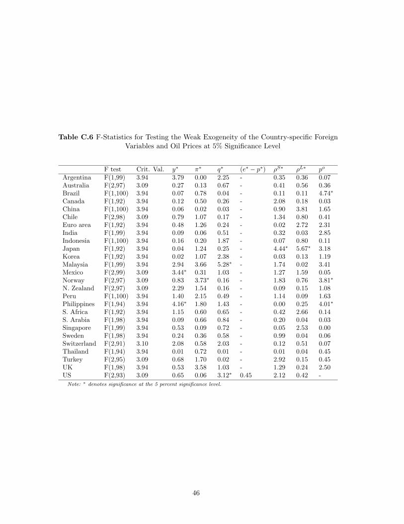
Table C.6 F-Statistics for Testing the Weak Exogeneity of the Country-specific ForeignVariables and Oil Prices at 5% Significance Level

F test Crit. Val. y∗ π∗ q∗ (e∗ − p∗) ρS∗ ρL∗ po

Argentina F(1,99) 3.94 3.79 0.00 2.25 - 0.35 0.36 0.07Australia F(2,97) 3.09 0.27 0.13 0.67 - 0.41 0.56 0.36Brazil F(1,100) 3.94 0.07 0.78 0.04 - 0.11 0.11 4.74∗

Canada F(1,92) 3.94 0.12 0.50 0.26 - 2.08 0.18 0.03China F(1,100) 3.94 0.06 0.02 0.03 - 0.90 3.81 1.65Chile F(2,98) 3.09 0.79 1.07 0.17 - 1.34 0.80 0.41Euro area F(1,92) 3.94 0.48 1.26 0.24 - 0.02 2.72 2.31India F(1,99) 3.94 0.09 0.06 0.51 - 0.32 0.03 2.85Indonesia F(1,100) 3.94 0.16 0.20 1.87 - 0.07 0.80 0.11Japan F(1,92) 3.94 0.04 1.24 0.25 - 4.44∗ 5.67∗ 3.18Korea F(1,92) 3.94 0.02 1.07 2.38 - 0.03 0.13 1.19Malaysia F(1,99) 3.94 2.94 3.66 5.28∗ - 1.74 0.02 3.41Mexico F(2,99) 3.09 3.44∗ 0.31 1.03 - 1.27 1.59 0.05Norway F(2,97) 3.09 0.83 3.73∗ 0.16 - 1.83 0.76 3.81∗

N. Zealand F(2,97) 3.09 2.29 1.54 0.16 - 0.09 0.15 1.08Peru F(1,100) 3.94 1.40 2.15 0.49 - 1.14 0.09 1.63Philippines F(1,94) 3.94 4.16∗ 1.80 1.43 - 0.00 0.25 4.01∗

S. Africa F(1,92) 3.94 1.15 0.60 0.65 - 0.42 2.66 0.14S. Arabia F(1,98) 3.94 0.09 0.66 0.84 - 0.20 0.04 0.03Singapore F(1,99) 3.94 0.53 0.09 0.72 - 0.05 2.53 0.00Sweden F(1,98) 3.94 0.24 0.36 0.58 - 0.99 0.04 0.06Switzerland F(2,91) 3.10 2.08 0.58 2.03 - 0.12 0.51 0.07Thailand F(1,94) 3.94 0.01 0.72 0.01 - 0.01 0.04 0.45Turkey F(2,95) 3.09 0.68 1.70 0.02 - 2.92 0.15 0.45UK F(1,98) 3.94 0.53 3.58 1.03 - 1.29 0.24 2.50US F(2,93) 3.09 0.65 0.06 3.12∗ 0.45 2.12 0.42 -

Note: ∗ denotes significance at the 5 percent significance level.

46

Table C.7 Number of Rejections of the Null of Parameter Constancy per Variable Across the

Country-specific Models at the 5 % Significance Level

Test y π q (e− p) ρS ρL Total

PKsup 10 5 4 2 4 1 26PKmsq 9 3 1 2 2 1 18N 5 3 5 10 3 4 30robust-N 4 2 1 7 1 2 17QLR 6 10 9 13 12 5 55robust-QLR 2 5 4 8 1 4 24MW 5 5 5 10 2 5 32robust-MW 5 5 5 10 2 4 31APW 6 9 9 12 12 6 54robust-APW 3 5 4 9 2 5 28Note: The test statistics PKsup and PKmsq are based on the cumulativesums of OLS residuals, N is the Nyblom test for time-varying parameters andQLR, MW and APW are the sequential Wald statistics for a single breakat an unknown change point. Statistics with the prefix ‘robust’ denote theheteroskedasticity-robust version of the tests. All tests are implemented at the5% significance level.

47

Table C.8 Break Dates Computed with the Quandt’s Likelihood Ratio Statistic (QLR) at the 5%

Significance Level

Variables y π q (e− p) ρS ρL po

Argentina 1989Q3 1989Q3 1989Q4 1989Q2 1989Q3 - -Australia 1989Q1 1987Q3 1987Q4 2000Q1 1987Q1 1989Q1 -Brazil 1990Q1 1989Q3 - 1999Q1 1989Q3 - -Canada 1987Q1 2001Q3 2000Q4 2001Q3 1987Q1 1997Q3 -China 2002Q2 1988Q3 - 1991Q1 1990Q1 - -Chile 1987Q1 1987Q1 1987Q3 2000Q4 1987Q4 - -Euro area 1987Q4 1990Q1 1992Q3 1998Q4 1988Q3 1989Q2 -India 1996Q2 1997Q3 1992Q2 2002Q1 1994Q4 - -Indonesia 1998Q1 1997Q4 - 1997Q2 1995Q1 - -Japan 1991Q1 1987Q1 1993Q1 1995Q2 1987Q3 1995Q4 -Korea 1998Q2 1987Q3 1997Q2 1998Q1 1998Q3 1987Q1 -Malaysia 1997Q3 2002Q2 1998Q3 1997Q2 1998Q2 - -Mexico 1988Q3 1988Q1 - 1995Q1 1988Q1 - -Norway 2001Q2 2000Q4 1990Q1 2002Q1 1998Q4 1990Q4 -N. Zealand 1987Q2 1987Q1 1991Q2 2000Q3 1987Q2 1987Q2 -Peru 1990Q1 1989Q4 - 1989Q4 1989Q4 - -Philippines 1987Q4 1987Q1 1987Q1 1987Q3 1987Q1 - -S. Africa 1987Q1 1994Q2 1988Q1 1989Q1 1997Q4 1989Q3 -S. Arabia 1990Q2 1997Q3 - 1995Q2 - - -Singapore 1997Q3 1989Q4 1991Q3 1997Q3 1995Q3 - -Sweden 1987Q1 1993Q2 1988Q1 2000Q1 1991Q1 1988Q1 -Switzerland 1987Q1 1987Q3 1987Q4 1992Q4 1989Q2 2001Q3 -Thailand 1993Q2 1992Q4 1990Q3 1997Q4 1994Q4 - -Turkey 1993Q4 1994Q2 - 2000Q4 1994Q2 - -UK 1987Q1 1990Q4 1987Q1 1988Q4 1987Q4 1987Q1 -US 1987Q1 2000Q4 2000Q3 - 1987Q1 1988Q2 1998Q4

48

Table C.9 Contemporaneous Effects of Foreign Variables on Domestic Counterparts byCountries

y π q (e− p) ρS ρL

Argentina 0.83 -0.04 1.26 - 1.61 -(0.22) (2.36) (0.40) - (2.40) -

Australia 0.34 0.77 0.81 - 0.45 0.89(0.12) (0.18) (0.14) - (0.11) (0.15 )

Brazil 0.59 3.30 - - 0.46 -(0.23) (2.52) - - (4.10) -

Canada 0.48 0.68 0.94 - 0.51 1.04(0.09) (0.11) (0.05) - (0.17) (0.07)

China 0.71 0.64 - - 0.02 -(0.22) (0.29) - - (0.04) -

Chile 0.77 0.11 0.51 - 0.13 -(0.24) (0.07) (0.12) - (0.07) -

Euro area 0.42 0.18 1.02 - 0.09 0.69(0.09) (0.08) (0.04) - (0.02) (0.08)

India 0.06 0.68 0.78 - -0.04 -(0.14) (0.33) (0.14) - (0.07) -

Indonesia 0.99 0.86 - - 0.98 -(0.41) (0.69) - - (0.83) -

Japan 0.10 0.10 0.72 - -0.05 0.50(0.16) (0.09) (0.10) - (0.05) (0.08)

Korea -0.08 0.70 0.94 - -0.21 0.21(0.19) (0.29) (0.17) - (0.13) (0.32)

Malaysia 1.26 0.61 1.11 - 0.00 -(0.34) (0.17) (0.20) - (0.09) -

Mexico 0.63 0.77 - - 0.01 -(0.17) (0.56) - - (0.54) -

Norway 1.33 0.78 1.14 - 0.36 0.70(0.31) (0.20) (0.09) - (0.20) (0.15)

N. Zealand 0.33 0.42 0.82 - 0.51 0.39(0.19) (0.18) (0.11) - (0.28) (0.22)

Peru 0.15 -0.58 - - -2.38 -(0.43) (2.44) - - (1.26) -

Philippines 0.03 -0.24 1.02 - 0.30 -(0.22) (0.52) (0.20) - (0.32) -

S. Africa 0.16 0.15 0.90 - 0.01 0.44(0.14) (0.24) (0.14) - (0.07) (0.22)

S. Arabia 0.42 0.11 - - - -(0.37) (0.20) - - - -

Singapore 0.86 0.32 1.27 - 0.27 -(0.25) (0.17) (0.12) - (0.14) -

Sweden 1.36 1.31 1.23 - 0.40 0.94(0.28) (0.16) (0.09) - (0.17) (0.16)

Switzerland 0.53 0.37 0.91 - 0.19 0.47(0.13) (0.10) (0.06) - (0.08) (0.08)

Thailand 0.33 0.63 0.83 - 0.37 -(0.20) (0.32) (0.12) - (0.27) -

Turkey 1.21 3.57 - - 1.10 -(0.42) (1.26) - - (0.77) -

UK 0.58 0.78 0.86 - 0.22 0.76(0.14) (0.12) (0.06) - (0.12) (0.12)

US 0.45 0.50 - - 0.01 -(0.12) (0.11) - - (0.05) -

Note: White’s heteroscedastic-robust standard errors are given in brackets.

49

Tab

leC

.10

Ave

rage

Pai

rwis

eC

ross

-sec

tion

Cor

rela

tion

sof

Rea

lG

DP

,In

flat

ion

,an

dE

qu

ity

Pri

cean

dA

ssoci

ated

Mod

el’s

Res

idu

als

Real

GD

PIn

flati

on

Equit

yP

rice

Lev

els

Fir

stV

AR

VA

RX

*L

evel

sF

irst

VA

RV

AR

X*

Lev

els

Fir

stV

AR

VA

RX

*D

iff.

Res

.R

es.

Diff

.R

es.

Res

.D

iff.

Res

.R

es.

Arg

enti

na

0.8

90.0

80.0

30.0

1A

rgen

tina

0.2

60.0

50.0

50.0

1A

rgen

tina

0.4

50.2

10.1

70.0

0A

ust

ralia

0.9

70.1

60.1

20.0

2A

ust

ralia

0.3

40.0

80.0

5-0

.02

Aust

ralia

0.7

90.5

20.4

70.0

5B

razi

l0.9

60.1

50.1

00.0

1B

razi

l0.2

10.0

10.0

0-0

.05

Bra

zil

--

--

Canada

0.9

70.2

00.1

00.0

2C

anada

0.4

10.1

40.1

10.0

2C

anada

0.7

30.5

40.4

80.0

5C

hin

a0.9

70.0

90.0

6-0

.02

Chin

a0.1

00.0

70.0

60.0

0C

hin

a-

--

-C

hile

0.9

60.1

60.0

90.0

2C

hile

0.3

90.0

5-0

.02

-0.0

1C

hile

0.7

80.2

90.2

80.0

6E

uro

are

a0.9

60.2

60.1

60.0

1E

uro

are

a0.4

60.1

60.1

30.0

3E

uro

are

a0.7

80.5

60.5

2-0

.10

India

0.9

7-0

.02

-0.0

1-0

.01

India

0.1

90.0

30.0

60.0

1In

dia

0.7

70.3

20.2

90.0

0In

dones

ia0.9

60.1

00.0

6-0

.01

Indones

ia0.0

10.0

40.0

70.0

2In

dones

ia-

--

-Japan

0.9

00.1

60.0

6-0

.03

Japan

0.4

20.0

90.0

5-0

.01

Japan

0.4

30.4

40.3

2-0

.11

Kore

a0.9

50.1

30.0

60.0

2K

ore

a0.3

70.0

60.0

50.0

0K

ore

a0.7

00.3

60.3

0-0

.02

Mala

ysi

a0.9

60.2

10.1

30.0

2M

ala

ysi

a0.2

70.1

10.0

90.0

1M

ala

ysi

a0.6

00.3

90.3

80.0

6M

exic

o0.9

60.1

70.1

20.0

2M

exic

o0.1

90.0

10.0

20.0

0M

exic

o-

--

-N

orw

ay0.9

70.1

20.1

10.0

3N

orw

ay0.3

70.0

80.0

60.0

3N

orw

ay0.8

10.4

90.4

60.0

6N

.Z

eala

nd

0.9

60.1

80.1

00.0

6N

.Z

eala

nd

0.3

30.0

70.0

40.0

3N

.Z

eala

nd

0.5

40.4

00.3

70.0

2P

eru

0.8

50.0

60.0

60.0

1P

eru

0.2

3-0

.04

0.0

0-0

.03

Per

u-

--

-P

hilip

pin

es0.9

40.0

70.0

30.0

1P

hilip

pin

es0.2

10.0

30.0

30.0

0P

hilip

pin

es0.7

20.3

60.3

40.0

3S.

Afr

ica

0.9

40.2

00.1

10.0

5S.

Afr

ica

0.3

30.0

60.0

40.0

4S.

Afr

ica

0.7

90.4

70.4

10.0

7S.

Ara

bia

0.8

90.0

30.0

5-0

.02

S.

Ara

bia

0.0

50.0

00.0

60.0

3S.

Ara

bia

--

--

Sin

gap

ore

0.9

60.2

00.1

40.0

0Sin

gap

ore

0.3

00.0

60.0

70.0

1Sin

gap

ore

0.7

30.5

30.4

90.0

1Sw

eden

0.9

60.2

10.1

60.0

1Sw

eden

0.4

60.1

00.1

10.0

1Sw

eden

0.7

70.5

00.4

7-0

.02

Sw

itze

rland

0.9

60.2

00.1

10.0

0Sw

itze

rland

0.3

90.0

90.0

70.0

2Sw

itze

rland

0.7

90.5

30.5

10.0

1T

hailand

0.9

40.1

80.0

70.0

2T

hailand

0.3

10.0

60.0

2-0

.01

Thailand

0.6

40.3

90.3

60.0

6T

urk

ey0.9

60.1

30.0

80.0

0T

urk

ey0.1

40.0

00.0

4-0

.01

Turk

ey-

--

-U

K0.9

70.2

10.1

50.0

3U

K0.4

50.1

10.1

20.0

2U

K0.7

70.5

50.5

0-0

.05

US

0.9

70.2

20.1

1-0

.02

US

0.4

20.1

90.1

60.0

1U

S0.7

80.5

40.4

8-0

.02

No

te:

VA

RX

*R

es(V

AR

X*

Res

idu

als

)re

fer

tore

sid

ua

lsfr

om

the

cou

ntr

ysp

ecifi

cV

AR

X*

mod

els

wit

hfo

reig

nva

ria

bles

,es

tim

ate

din

the

firs

tst

epo

fG

VA

Ra

na

lysi

s.T

he

nu

mbe

ro

fco

inte

gra

tio

nre

lati

on

sa

nd

lag

ord

ers

inth

eco

un

try

spec

ific

VA

RX

*m

odel

sa

regi

ven

inT

abl

eC

.1.

VA

RR

es(V

AR

Res

idu

als

)a

reo

bta

ined

aft

erre

-est

ima

tin

ga

llth

ein

div

idu

al

cou

ntr

y-s

peci

fic

mod

els

ove

rth

esa

me

peri

odex

clu

din

gth

efo

reig

nva

ria

bles

,in

clu

din

go

ila

sen

dog

eno

us

ina

llth

eco

un

try

mod

els.

Fo

rea

chco

un

try

VA

Rm

odel

we

use

dth

esa

me

lag

ord

era

ssp

ecifi

edin

Ta

ble

C.1

an

dse

lect

edth

en

um

ber

of

coin

tegr

ati

on

rela

tio

nsh

ips

base

do

nth

eJ

oh

an

sen’

str

ace

sta

tist

ics

com

pu

ted

for

the

ind

ivid

ua

lV

AR

mod

els

excl

ud

ing

the

fore

ign

vari

abl

es.

50

Tab

leC

.11

Ave

rage

Pai

rwis

eC

ross

-sec

tion

Cor

rela

tion

sof

Exch

ange

Rat

e,S

hor

t-te

rman

dL

ong-

term

Inte

rest

Rat

ean

dA

ssoci

ated

Mod

el’s

Res

idu

als

Real

Exch

ange

Rate

Short

-term

Inte

rest

Rate

Long-t

erm

Inte

rest

Rate

Lev

els

Fir

stV

AR

VA

RX

*L

evel

sF

irst

VA

RV

AR

X*

Lev

els

Fir

stV

AR

VA

RX

*D

iff.

Res

.R

es.

Diff

.R

es.

Res

.D

iff.

Res

.R

es.

Arg

enti

na

0.4

20.0

90.0

70.0

7A

rgen

tina

0.4

20.0

30.0

2-0

.02

Arg

enti

na

--

--

Aust

ralia

0.7

60.3

60.3

00.2

4A

ust

ralia

0.5

50.1

30.0

80.0

0A

ust

ralia

0.8

50.3

70.2

80.0

2B

razi

l0.7

00.1

80.1

30.1

1B

razi

l0.3

60.0

10.0

0-0

.07

Bra

zil

--

--

Canada

0.7

20.3

10.2

10.1

8C

anada

0.6

00.1

80.1

50.1

0C

anada

0.8

70.3

70.3

2-0

.01

Chin

a0.1

90.0

80.0

30.0

2C

hin

a0.4

90.0

70.0

50.0

2C

hin

a-

--

-C

hile

0.6

40.2

70.2

10.1

6C

hile

0.5

70.0

2-0

.05

-0.0

4C

hile

--

--

Euro

are

a0.7

50.3

60.3

00.3

2E

uro

are

a0.6

10.1

80.1

00.0

5E

uro

are

a0.8

60.4

50.3

4-0

.05

India

0.3

30.2

40.2

10.1

7In

dia

0.3

40.1

00.0

50.0

4In

dia

--

--

Indones

ia0.0

50.2

20.1

40.1

2In

dones

ia0.1

50.0

80.0

70.0

4In

dones

ia-

--

-Japan

0.6

40.1

70.1

40.1

6Japan

0.5

70.0

50.0

20.0

0Japan

0.8

30.2

80.2

3-0

.04

Kore

a0.7

30.2

80.2

20.1

7K

ore

a0.5

40.0

60.0

50.0

5K

ore

a0.7

50.0

60.0

2-0

.05

Mala

ysi

a0.6

20.2

90.2

30.2

1M

ala

ysi

a0.4

30.0

60.0

20.0

5M

ala

ysi

a-

--

-M

exic

o0.6

50.0

80.0

40.0

0M

exic

o0.4

30.0

30.0

20.0

4M

exic

o-

--

-N

orw

ay0.7

50.3

80.3

40.3

3N

orw

ay0.5

50.0

5-0

.02

-0.0

1N

orw

ay0.8

30.2

70.2

2-0

.01

N.

Zea

land

0.7

50.3

60.3

00.2

7N

.Z

eala

nd

0.4

90.0

60.0

50.0

1N

.Z

eala

nd

0.7

60.1

90.1

20.0

2P

eru

0.7

00.0

50.0

60.0

5P

eru

0.4

00.0

40.0

40.0

5P

eru

--

--

Philip

pin

es0.7

30.1

80.1

80.1

6P

hilip

pin

es0.5

60.0

90.0

50.0

3P

hilip

pin

es-

--

-S.

Afr

ica

0.6

40.3

00.2

50.2

4S.

Afr

ica

0.3

90.1

10.0

60.0

4S.

Afr

ica

0.5

30.1

90.1

30.0

0S.

Ara

bia

0.4

40.0

70.0

50.0

7S.

Ara

bia

--

--

S.

Ara

bia

--

--

Sin

gap

ore

0.7

40.3

70.3

00.2

6Sin

gap

ore

0.5

10.0

90.0

80.0

2Sin

gap

ore

--

--

Sw

eden

0.7

00.3

50.2

90.2

8Sw

eden

0.6

40.1

00.0

70.0

2Sw

eden

0.8

70.3

70.2

80.0

2Sw

itze

rland

0.7

40.3

00.2

50.3

0Sw

itze

rland

0.4

50.0

90.0

2-0

.02

Sw

itze

rland

0.7

40.3

70.2

10.0

1T

hailand

0.7

30.2

90.2

50.2

2T

hailand

0.5

60.1

20.0

80.0

4T

hailand

--

--

Turk

ey0.7

30.1

90.1

30.0

7T

urk

ey0.1

50.0

50.0

40.0

1T

urk

ey-

--

-U

K0.7

30.3

40.2

80.2

6U

K0.6

10.1

50.0

90.0

4U

K0.8

60.3

90.2

8-0

.04

US

--

--

US

0.5

20.1

10.0

80.0

3U

S0.8

30.4

00.3

0-0

.02

No

te:

VA

RX

*R

es(V

AR

X*

Res

idu

als

)re

fer

tore

sid

ua

lsfr

om

the

cou

ntr

ysp

ecifi

cV

AR

X*

mod

els

wit

hfo

reig

nva

ria

bles

,es

tim

ate

din

the

firs

tst

epo

fG

VA

Ra

na

lysi

s.T

he

nu

mbe

ro

fco

inte

gra

tio

nre

lati

on

sa

nd

lag

ord

ers

inth

eco

un

try

spec

ific

VA

RX

*m

odel

sa

regi

ven

inT

abl

eC

.1.

VA

RR

es(V

AR

Res

idu

als

)a

reo

bta

ined

aft

erre

-est

ima

tin

ga

llth

ein

div

idu

al

cou

ntr

y-s

peci

fic

mod

els

ove

rth

esa

me

peri

odex

clu

din

gth

efo

reig

nva

ria

bles

,in

clu

din

go

ila

sen

dog

eno

us

ina

llth

eco

un

try

mod

els.

Fo

rea

chco

un

try

VA

Rm

odel

we

use

dth

esa

me

lag

ord

era

ssp

ecifi

edin

Ta

ble

C.1

an

dse

lect

edth

en

um

ber

of

coin

tegr

ati

on

rela

tio

nsh

ips

base

do

nth

eJ

oh

an

sen’

str

ace

sta

tist

ics

com

pu

ted

for

the

ind

ivid

ua

lV

AR

mod

els

excl

ud

ing

the

fore

ign

vari

abl

es.

51

Figure C.2 GIRFs for One Standard Deviation Increase in China GDP(World economy and LAC5; Bootstrapped GIRFs, 2009)

52

Figure C.3 GIRFs for One Standard Deviation Increase in China GDP(World economy and LAC5; Bootstrapped GIRFs, 1985)

53

Figure C.4 GIRFs for One Standard Deviation Increase in US GDP(World economy and LAC5; Bootstrapped GIRFs, 2009)

54

Figure C.5 GIRFs for One Standard Deviation Increase in US GDP(World economy and LAC5; Bootstrapped GIRFs, 1985)

55

Figure C.6 GIRFs for One Standard Deviation Increase in LAC5 GDP(World economy and LAC5; Bootstrapped GIRFs, 2009)

56

Figure C.7 GIRFs for One Standard Deviation Increase in LAC5 GDP(World economy and LAC5; Bootstrapped GIRFs, 1985)

57

Figure C.8 GIRFs for One Standard Deviation Increase in rest of Asia GDP(World economy and LAC5; Bootstrapped GIRFs, 2009)

58

Figure C.9 GIRFs for One Standard Deviation Increase in rest of Asia GDP(World economy and LAC5; Bootstrapped GIRFs, 1985)

59

References

Andrews, D. W. K., and W. Ploberger (1994): “Optimal Tests When a Nuisance Parameter IsPresent Only under the Alternative,” Econometrica, 62(6), 1383–1414.

Brown, R. L., J. Durbin, and J. M. Evans (1975): “Techniques for Testing the Constancy of Re-gression Relationships over Time,” Journal of the Royal Statistical Society. Series B (Methodological),37(2), pp. 149–192.

Calderon, C. (2008): “The Growth of China and India Is Not a Zero-Sum Game for Latin America andthe Caribbean:Short- and Long-Term Effects,” in China’s and India’s Challenge to Latin America.Opportunity or threat?, ed. by M. Olarreaga, G. Perry, and D. Lederman, pp. 39–100. The WorldBank Press.

Canova, F. (2005): “The transmission of US shocks to Latin America,” Journal of Applied Economet-rics, 20(2), 229–251.

Cesa-Bianchi, A., A. Powell, and A. Rebucci (2011): “Exuberance crises,” Unpublishedmanuscript, Inter-American Development Bank, Washington DC.

Cesa-Bianchi, A., and A. Rebucci (2011): “Housing Cycles in the Global Economy,” Unpublishedmanuscript, Inter-American Development Bank, Washington DC.

Cova, P., M. Pisani, and A. Rebucci (2010): “Macroeconomic Effects of China’s Fiscal Stimulus,”RES Working Papers 4689, Inter-American Development Bank, Research Department.

Dees, S., F. di Mauro, M. H. Pesaran, and L. V. Smith (2007): “Exploring the internationallinkages of the euro area: a global VAR analysis,” Journal of Applied Econometrics, 22(1), 1–38.

Dees, S., M. H. Pesaran, L. V. Smith, and R. P. Smith (2010): “Supply, Demand and MonetaryPolicy Shocks in a Multi-Country New Keynesian Model,” Working Paper Series 1239, EuropeanCentral Bank.

Devlin, R., A. Estevadeordal, and A. Rodriguez-Clare (2006): The Emergence of China:Opportunities and Challenges for Latin America and the Caribbean. Harvard University Press.

Elliott, G., T. J. Rothenberg, and J. H. Stock (1996): “Efficient Tests for an AutoregressiveUnit Root,” Econometrica, 64(4), 813–36.

Garratt, A., K. Lee, M. H. Pesaran, and Y. Shin (2006): Global and National Macroeconometricmodelling. Oxford University Press.

Hansen, B. E. (2002): “Tests for Parameter Instability in Regressions with I(1) Processes,” Journalof Business and Economic Statistics, 20(1), pp. 45–59.

Harbo, I., S. Johansen, B. Nielsen, and A. Rahbek (1998): “Asymptotic Inference on Cointe-grating Rank in Partial Systems,” Journal of Business & Economic Statistics, 16(4), 388–99.

Hoffmaister, A. W., and J. Roldos (1997): “Are Business Cycles Different in Asia and LatinAmerica?,” IMF Working Papers 97/9, International Monetary Fund.

Izquierdo, A., R. Romero, and E. Talvi (2008): “Booms and Busts in Latin America: TheRole of External Factors,” RES Working Papers 4569, Inter-American Development Bank, ResearchDepartment.

Izquierdo, A., and E. Talvi (2011): One Region, Two Speeds? Challenges of the New GlobalEconomic Order for Latin America and the Caribbean. Inter-American Development Bank.

60

Johansen, S. (1992): “Cointegration in partial systems and the efficiency of single-equation analysis,”Journal of Econometrics, 52(3), 389–402.

Koop, G., M. H. Pesaran, and S. M. Potter (1996): “Impulse response analysis in nonlinearmultivariate models,” Journal of Econometrics, 74(1), 119–147.

Kose, M. A., and E. Prasad (2010): Emerging markets: resilience and growth amid global turmoil.Brookings Institution Press.

Leybourne, S., T.-H. Kim, and P. Newbold (2005): “Examination of Some More Powerful Modi-fications of the Dickey-Fuller Test,” Journal of Time Series Analysis, 26(3), 355–369.

Little, I. M. D., R. N. Cooper, W. M. Corden, and S. Rajapatirana (1993): Boom, Crisis,and Adjustment: The Macreconomic Experience of Developing Countries. Oxford University Press,New York.

MacKinnon, J. G. (1991): “Critical values for cointegration tests,” in Long-Run Economic Relation-ships: Readings in Cointegration, ed. by R. F. Engle, and C. W. J. Granger, chap. 13.

Mizon, G. E., and D. F. Hendry (1998): “Exogeneity, causality, and co-breaking in economic policyanalysis of a small econometric model of money in the UK,” Empirical Economics, 23(3), 267–294.

Nyblom, J. (1989): “Testing for the Constancy of Parameters Over Time,” Journal of the AmericanStatistical Association, 84(405), pp. 223–230.

Osterholm, P., and J. Zettelmeyer (2007): “The Effect of External Conditions on Growth inLatin America,” IMF Working Papers 07/176, International Monetary Fund.

Pantula, S. G., G. Gonzalez-Farias, and W. A. Fuller (1994): “A Comparison of Unit-RootTest Criteria,” Journal of Business & Economic Statistics, 12(4), 449–59.

Park, H. J., and W. A. Fuller (1995): “Alternative estimators and unit root tests for the autore-gressive process,” Journal of Time Series Analysis, 16(4), 415–429.

Pesaran, M. H. (2006): “Estimation and Inference in Large Heterogeneous Panels with a MultifactorError Structure,” Econometrica, 74(4), 967–1012.

Pesaran, M. H., and B. Pesaran (2009): Time Series Econometrics using Microfit 5.0: A User’sManual. Oxford University Press.

Pesaran, M. H., T. Schuermann, and L. V. Smith (2009a): “Forecasting economic and financialvariables with global VARs,” International Journal of Forecasting, 25(4), 642–675.

(2009b): “Rejoinder to comments on forecasting economic and financial variables with globalVARs,” International Journal of Forecasting, 25(4), 703–715.

Pesaran, M. H., T. Schuermann, and S. Weiner (2004): “Modeling Regional Interdependen-cies Using a Global Error-Correcting Macroeconometric Model,” Journal of Business & EconomicStatistics, 22, 129–162.

Pesaran, M. H., and Y. Shin (1996): “Cointegration and speed of convergence to equilibrium,”Journal of Econometrics, 71(1-2), 117–143.

(1998): “Generalized impulse response analysis in linear multivariate models,” EconomicsLetters, 58(1), 17–29.

Pesaran, M. H., Y. Shin, and R. J. Smith (2000): “Structural analysis of vector error correctionmodels with exogenous I(1) variables,” Journal of Econometrics, 97(2), 293 – 343.

61

Ploberger, W., and W. Kramer (1992): “The CUSUM Test with OLS Residuals,” Econometrica,60(2), 271–85.

Quandt, R. E. (1960): “Tests of the Hypothesis that a Linear Regression System Obeys Two SeparateRegimes,” Journal of the American Statistical Association, 55(290), pp. 324–330.

Rebucci, A. (1998): “External Shocks, Macroeconomic Policy, and Growth: A Panel VAR Approach,”Global Economic Institutions (GEI) Working Paper, CEPR, London 40.

Xu, T. (2010): “The role of credit in international business cycles,” Unpublished manuscript, Cam-bridge University.

62