Embed Size (px)
Citation preview
Potential Analysishttps://doi.org/10.1007/s11118-018-9754-y
Electrostatic Problems with a Rational Constraintand Degenerate Lame Equations
Dimitar K. Dimitrov1 ·Boris Shapiro2
Received: 6 October 2017 / Accepted: 3 December 2018© The Author(s) 2018
AbstractIn this note we extend the classical relation between the equilibrium configurations of unitmovable point charges in a plane electrostatic field created by these charges together withsome fixed point charges and the polynomial solutions of a corresponding Lame differentialequation. Namely, we find similar relation between the equilibrium configurations of unitmovable charges subject to a certain type of rational or polynomial constraint and polyno-mial solutions of a corresponding degenerate Lame equation, see details below. In particular,the standard linear differential equations satisfied by the classical Hermite and Laguerrepolynomials belong to this class. Besides these two classical cases, we present a number ofother examples including some relativistic orthogonal polynomials and linear differentialequations satisfied by those.
Keywords Electrostatic equilibrium · Lame differential equation
Mathematics Subject Classification (2010) Primary 31C10 · 33C45
To Heinrich Eduard Heine and Thomas Joannes Stieltjes whose mathematics continues to inspire aftermore than a century
Research supported by the Brazilian Science Foundations FAPESP under Grants 2016/09906-0 and2017/02061-8 and CNPq under Grant 306136/2017-1.
� Boris [email protected]
Dimitar K. [email protected]
1 Departamento de Matematica Aplicada, IBILCE, Universidade Estadual Paulista, 15054-000 SaoJose do Rio Preto, SP, Brazil
2 Department of Mathematics, Stockholm University, SE-106 91 Stockholm, Sweden
/
(2020) 52:645–659
Published online: 18 2018December

1 Introduction
For a given configuration of p + 1 fixed point charges νj located at the fixed points aj ∈ C
and n unit movable charges located at the variable points xk ∈ C, k = 1, . . . , n respectively,the (logarithmic) energy of this configuration is given by
L(x1, . . . , xn) = −n∑
k=1
p∑
j=0
νj log |aj − xk| −∑
1≤i<k≤n
log |xk − xi |. (1.1)
The standard electrostatic problem in this set-up is as follows.
Problem 1 Find/count all equilibrium configurations of movable charges, i.e., all thecritical points of the energy function L(x1, . . . , xn).
The above electrostatic problem has been initially studied by H. E. Heine [4] andT. J. Stieltjes [12] and is now commonly known as the classical Heine-Stieltjes electrostaticproblem. Besides Heine and Stieltjes, the latter question has been considered by F. Klein [5],E. B. Van Vleck [16], G. Szego [13], and G. Polya [10], just to mention a few. A relativelyrecent survey of results on the classical Heine-Stieltjes problems can be found in [11]. Thegeneral case of arbitrary movable charges is much less studied due to the missing relationwith linear ordinary differential equations, but the case when all movable charges are of thesame sign was, in particular, considered by A. Varchenko in [14].
Theorem A (Stieltjes’ theorem, [12]) If all p + 1 fixed positive charges are placed on thereal line, then for each of the (n+p−1)!/(n!(p−1)!) possible placements of n unit movablecharges in p finite intervals of the real axis bounded by the fixed charges, the classicalHeine-Stieltjes problem possesses a unique solution.
Heine’s major result from [4] claims that in the situation with p + 1 fixed and n unitmovable charges, the number of equilibrium configurations (assumed finite) can not exceed(n + p − 1)!/(n!(p − 1)!), see Theorem B below. Therefore, the above Stieltjes’ theo-rem describes all possible equilibrium configurations occurring under the assumptions ofTheorem A.
The most essential observation of the Heine-Stieltjes theory is that in case of equal mov-able charges, each equilibrium configuration is described by a polynomial solution of aLame differential equation. Recall that a Lame equation (in its algebraic form) is given by
A(x)y′′ + 2B(x)y′ + V (x)y = 0, (1.2)
where A(x) = (x − a0) · · · (x − ap) and B(x) is a polynomial of degree at most p such that
B(x)
A(x)=
p∑
j=0
νj
x − aj
(1.3)
and V (x) is a polynomial of degree at most p − 1.In this set-up the general Heine-Stieltjes electrostatic problem is equivalent to the
following question about the corresponding Lame equation:
Problem 2 Given polynomials A(x) and B(x) as above, and a positive integer n, find allpossible polynomials V (x) of degree at most p − 1 for which Eq. 1.2 has a polynomialsolution y of degree n.
D.K. Dimitrov, B. Shapiro646

Heine’s original result was formulated in this language and it claims the following.
Theorem B (Heine [4], see also [11]) If the coefficients of the polynomials A(x) and B(x)
are algebraically independent numbers, i.e., they do not satisfy an algebraic equation withinteger coefficients, then for any integer n > 0, there exist exactly
(n+p−1
n
)polynomials
V (x) of degree p−1 such that the Eq. 1.2 has a unique (up to a constant factor) polynomialsolution y of degree n.
Polynomial V (x) solving Problem 2 is called a Van Vleck polynomial of the latter prob-lem while the corresponding polynomial solution y(x) is called the Stieltjes polynomialcorresponding to V (x).
The relation between Problem 1 and Problem 2 in case of equal movable charges is verystraightforward. Namely, given the locations and values (aj , νj ), j = 0, . . . , p of the fixedcharges and the number n of the movable unit charges, every equilibrium configuration ofthe movable charges is exactly the set of all zeros of some Stieltjes polynomial y(x) ofdegree n for Problem 2.
In the particular case of p = 1, a0 = −1, a1 = 1, ν0 = (β+1)/2 and ν1 = (α+1)/2, thisinterpretation explains why the unique equilibrium position of n unit movable charges in theinterval (−1, 1) is determined by the fact that the set {xk}, k = 1, . . . , n coincides with thezero locus of the Jacobi polynomial P
(α,β)n (x). (Recall that {P (α,β)
n (x)} is the sequence ofpolynomials, orthogonal on [−1, 1] with respect to the weight function (1 − x)α(1 + x)β .)
The main goal of this note is to find the electrostatic interpretation of the zeros of poly-nomial solutions of Problem 2 for a more general class of Lame equations when there isno restriction deg A(x) > deg B(x). Namely, we say that a linear second order differentialoperator
d = A(x)d2
dx2+ 2B(x)
d
dx, (1.4)
with polynomial coefficients A(x) and B(x) is a non-degenerate Lame operator ifdeg A(x) > deg B(x) and a degenerate Lame operator otherwise. The Fuchs index fd ofthe operator d is, by definition, given by
fd := max(deg A(x) − 2, deg B(x) − 1).
For the Heine-Stieltjes problem to be well-defined, we consider below Lame operators T
with fd ≥ 0. For such operators, Problem 2 with Eq. 1.2 makes perfect sense. In otherwords, we are looking for Van Vleck polynomials V (x) of degree at most fd such thatEq. 1.2 has a polynomial solution of a given degree n. We call (1.2) with a degenerate
Lame operator d = A(x) d2
dx2 + B(x) ddx
and V (x) of degree at most fd, a degenerate Lameequation.
The most well-known examples of such equations are those satisfied by the Hermiteand the Laguerre polynomials. Namely, the Hermite and the Laguerre polynomials arepolynomial solutions of the second order differential equations:
y′′ − 2x y′ + 2n y = 0, y(x) = Hn(x), (1.5)
x y′′ + (α + 1 − x) y′ + n y = 0, y(x) = Lαn(x). (1.6)
Obviously, Eqs. 1.5 and 1.6 are degenerate Lame equations with Fuchs index 0. Dueto this fact, the classical interpretation of the zeros of the Hermite and the Laguerre poly-nomials as coordinates of the critical points of the energy function (1.1) does not apply.
Electrostatic Problems with a Rational Constraint and Degenerate... 647
Nevertheless, as was already observed by G. Szego [13], the zeros of the Hermite andthe Laguerre polynomials still possess a nice electrostatic interpretation in terms of theminimum of the energy function (1.1) subject to certain polynomial constraints.
Theorem C ([13], Theorems 6.7.2 and 6.7.3) (i) The zeros of the Hermite polynomialHn(c2x), c2 = √
(n − 1)/2M, M > 0, form an equilibrium configuration of n unitcharges that obey the constraint x2
1 + · · ·+ x2n ≤ Mn without fixed charges. In partic-
ular, the zeros of Hn(x) form an equilibrium configuration of n unit charges subjectto the constraint x2
1 + · · · + x2n ≤ n(n − 1)/2.
(ii) The zeros of the Laguerre polynomial Lαn(c1x), c1 = (n + α)/K, K > 0, form an
equilibrium configuration of n unit movable charges that obey the additional con-straint x1 + · · ·+ xn ≤ Kn in the presence of one fixed charge ν0 = (α + 1)/2 placedat the origin. In particular, the zeros of L
(α)n (x) form an equilibrium configuration of
n unit charges satisfying the constraint x1 + · · · + xn ≤ n(n + α) in the electrostaticfield created by them together with the above fixed charge.
Remark 1 Due to homogeneity of the problem, one can easily conclude that it suffices toconsider only the case of equality in the above constraints.
From the first glance it seems difficult to relate the electrostatic problems of Theorem Cto the corresponding differential equation since e.g., in the case of the Hermite polynomials
B(x)/A(x) = −x
which has no non-trivial partial fraction decomposition.In order to do this, we restrict ourselves to degenerate Lame equations with all distinct
roots of A(x) and non-negative Fuchs index. Given such an equation, consider the classicalelectrostatic problem with all unit movable charges and assume that the positions X =(x1, . . . , xn) of the movable charges are subject to an additional constraint R(X) = 0 of aspecial form. Namely, we say that a rational function R(X) is A-adjusted if
R(X) := R(x1, . . . , xn) =n∑
k=1
r(xk), (1.7)
where r(x) is a fixed univariate rational function such that D(x) := A(x)r ′(x) is a polyno-mial. We will also call the univariate function r(x) satisfying the latter condition A-adjusted.In particular, if r(x) is an arbitrary polynomial, then Eq. 1.7 is automatically A-adjusted.
Given an A-adjusted rational function R(X), set
� = {X ∈ Cn : R(X) = 0}
and denote by A the hyperplane arrangement in Cn with coordinates (x1, . . . , xn) consisting
of all hyperplanes of the form {xi = aj } and {xi = x�} for i = 1, . . . , n, j = 0, . . . , p andi �= �. Here {a0, . . . , ap} is the set of roots of A(x) (assumed pairwise distinct).
Now consider the 1-parameter family of the Lame differential equations of the form
A(x)y′′ + (2B(x) − ρD(x))y′ + V (x)y = 0, (1.8)
depending on a complex-valued parameter ρ. We call (1.8) the parametric Lame equation.Consider an arbitrary degenerate Lame (1.2) with all distinct roots of A(x). Given an
A-adjusted rational function R(X), set q := deg D(x).
D.K. Dimitrov, B. Shapiro648

Theorem 1 (Stieltjes’ theorem with an A-adjusted constraint) In the above notation, theenergy function L(x) given by Eq. 1.1 and the parametric Lame (1.8) satisfy the following:
• Let X∗ = (x∗1 , . . . , x∗
n) be a vector lying in Cn \ A. Assume that X∗ satisfies the
constraint R(X∗) = 0 and is a critical point of the energy function L(X). Then thereexist a polynomial V (x) of degree max{p − 1, q − 1} and a constant ρ∗ such that
y(x) = (x − x∗1 ) · · · (x − x∗
n)
is a solution of the parametric Lame (1.8) with ρ = ρ∗.• Let V (x) be a polynomial satisfying the condition deg V ≤ max{p − 1, q − 1}, and ρ∗
be a constant for which the parametric Lame (1.8) possesses a polynomial solution ofthe form y(x) = (x − x∗
1 ) · · · (x − x∗n), such that X∗ = (x∗
1 , . . . , x∗n) ∈ � \ A. Then
∂L(X)
∂xk
∣∣∣∣X∗
− ρ∗
2
∂R(X)
∂xk
∣∣∣∣X∗
= 0, k = 1, . . . , n.
Here, by definition, ∂R(X)∂xk
∣∣∣X∗ := r ′(x∗
k ).
Remark 2 Additionally, if all fixed charges are positive and placed on the real line, and X∗is a point of a local minimum of L(X), then the constant ρ∗ must be positive.
Example 1 Observe that the above differential equations for the Hermite and Laguerre poly-nomials are nothing else but the parametric Lame equations for the appropriate values ofparameter ρ and they adequately describe the corresponding electrostatic problems. (Thecorresponding values of ρ are denoted by ρ∗.)
Namely, the Hermite polynomial Hn(x) is a solution of the differential (1.5) which can beinterpreted as a parametric Lame (1.8) with A(x) = 1, B(x) = 0, V (x) = 2n, D(x) = 2x,and ρ∗ = 1. The fact that A(x) = 1 and B(x) = 0 is equivalent to the absence of fixedcharges. In this case, R(X) = x2
1 + · · · + x2n − (n − 1)/2n which implies that
D(xk) := A(xk)∂R(X)
∂xk
= A(xk)r′(xk) = 2xk,
where r(x) = x2 − (n − 1)/2n2.Analogously, the differential (1.6) satisfied by the Laguerre polynomial L
(α)n (x) can be
interpreted as a parametric Lame (1.8) with A(x) = x, B(x) = (α + 1)/2, D(x) = 1, andρ∗ = 1. Then the partial fraction decomposition B(x)/A(x) = (α + 1)/2x indicates thepresence of one fixed charge (α + 1)/2 at the origin. In this case, R(X) = x1 + · · · + xn −(n + α)/n and
D(xk) := A(xk)∂R(X)
∂xk
= A(xk)r′(xk) = xk,
where r(x) = x − (n + α)/n2.
Theorem 1 allows us to formulate the main result of this note which provides a generalrelation between degenerate Lame equations and electrostatic problems in the presence ofan A-adjusted rational constraint.
Theorem 2 LetA(x)y′′ + B(x)y′ + V (x)y = 0, (1.9)
be a degenerate Lame equation, i.e., deg A(x) ≤ deg B(x) and deg V ≤ fd for d =A(x)y′′ + B(x)y′. Assume that all roots of A(x) are distinct and that r(x) is an A-adjusted
Electrostatic Problems with a Rational Constraint and Degenerate... 649

univariate rational function such that deg(B(x) + ρA(x)r ′(x)) < deg A(x) for at least onevalue of ρ. Set
B(x) := −ρ A(x)r ′(x) + 2B(x), R(X) = R(x1, . . . , xn) :=n∑
k=1
r(xk),
where ρ is an arbitrary complex constant. Then there exists a value ρ∗ of the constant ρ, forwhich the degenerate Lame (1.9) coincides with the parametric Lame equation correspond-ing to the electrostatic problem of Theorem 1 with fixed charges determined by the partialfraction decomposition of B(x)/A(x) and a polynomial constraint of the form R(X) = 0.
Theorem 1, and especially Theorem 2, together with the classical relation betweennondegenerate Lame equations and electrostatics, reveal a rather general phenomenon.Namely, every Lame differential (1.9) where A(x) has distinct complex zeros is relatedto an electrostatic problem no matter what the degree of the polynomial B(x) is, pro-vided only that the Fuch index is nonnegative. Indeed, dividing B(x) by A(x) we obtainB(x) = −ρ A(x)r ′(x)+2B(x). In the classical non-degenerate case when deg B < deg A,we have r ′(x) = 0 and the partial fraction decomposition of B(x)/A(x) determines thepositions and the strengths of all fixed charges. In the degenerate case, the A-adjusted func-tion r(x), satisfying the assumptions of Theorem 2, is simply a primitive of the quotientr ′(x). In other words, r(x) is a unique, up to an additive constant, polynomial with the aboveproperties.
However, in some situations r ′(x) is a rational function and not just a polynomial, seeSection 3.3 below. In many cases the value ρ∗ of the constant ρ is uniquely determined. Itis clear that r(x) is determined up to an additive constant of integration, so that one needs todetermine the value of the constant c, such that the zeros x∗
1 , . . . , x∗n of a polynomial solu-
tion y(x) satisfy the constraint∑n
k=1 r(x∗k ) + c = 0. Usually c is easily obtained either by
comparing the coefficients of certain powers of x in the corresponding Lame equation orwhen the Stjieltes polynomial is known explicitly, by explicit calculation of the correspond-ing quantities for the zeros of y(x) via Viete’s relations. The partial fraction decompositionof B(x)/A(X), where B(x) is the remainder in the above presentation of B(x), determinesthe fixed charges, if any.
2 Proofs
Consider the multi-valued analytic function
F(X) =p∏
j=0
n∏
i=1
(xi − aj )νj
∏
1≤i<j≤n
(xj − xi). (2.10)
F(X) is well-defined as a multi-valued function at least in Cn \A and also on some part of
A where it vanishes. (This function and its generalizations called the master functions werethoroughly studied by A. Varchenko and his coauthors in a large number of publicationsincluding [14, 15].) Although F(x) is multi-valued (unless all νj ’s are integers), its absolutevalue
H(X) := |F(X)| =p∏
j=0
n∏
i=1
|xi − aj |νj∏
1≤i<j≤n
|xj − xi |.
D.K. Dimitrov, B. Shapiro650

is a uni-valued function in Cn \A. Obviously, the energy function (1.1) satifies the relation
L(X) = − log H(x) = − log |F(X)|which implies that L(X) is a well-defined pluriharmonic function in C
n \ A, see e.g. [3].(If all νj ’s are positive, then L(x) is plurisuperharmonic function in C
n.)Although F(X) is multi-valued, its critical points in C
n \ A are given by a well-definedsystem of algebraic equations and are typically finitely many due to the fact that the ratioof any two branches is constant. (For degenerate cases, these critical points can formsubvarieties of positive dimension.) The following general fact is straightforward.
Lemma 1 Let fj : Ck → C, j = 1, . . . , N be pairwise distinct linear polynomials and let(y1, . . . , yk) be coordinates in Ck . For every j , denote by Hj ⊂ C
k the hyperplane given by{fj = 0} and set T = C
k \⋃Nj=1 Hj . Given a collection of complex numbers = {λj }Nj=1,
define
�(y1, . . . , yk) =N∏
j=1
fλj
j .
(� is a multi-valued holomorphic function defined in T .) Then the system of equationsdefining the critical points of � in T is given by:
N∑
j=1
λj
∂fj
∂y�
/fj = 0, � = 1, . . . , k.
(Note that by a critical point of a holomorphic function we mean a point where its com-plex gradient vanishes.) Similarly, for any algebraic hypersurface Y ⊂ C
k , the critical pointsof the restriction of � to Y ∩ T are well-defined independently of its branch and can befound by using the complex version of the method of Lagrange multipliers.
Lemma 2 In the notation of Lemma 1, let Y ⊂ Ck be an algebraic hypersurface given by
Q(y1, . . . , yk) = 0. Then the critical points of the restriction of � to Y ∩ T are given bythe condition that the gradient of the Lagrange function
L(y1, . . . , yk, ρ) = � − ρ
2Q(y1, . . . , yk)
vanishes, where ρ is a complex parameter. The latter condition is given by the system ofequations
N∑
j=1
λj
∂fj
∂y�
/fj = ρ
2
∂Q
∂y�
, � = 1, . . . , k, and Q(y1, . . . , yk) = 0. (2.11)
More exactly, if (y∗1 , . . . , y∗
k , ρ∗) solves (2.11), then (y∗1 , . . . , y∗
k ) is a critical point of �
restricted to Y ∩ T .
Proof If � were a well-defined holomorphic function defined in T and Y were as above,then the claim of Lemma 2 would be an immediate consequence of the method of Lagrangemultipliers.
In our situation, however, � is multi-valued, but the ratio of any two branches is a non-vanishing constant. This implies that at any point of T , the (complex) gradients of any twobranches are proportional to each other with a non-vanishing constant of proportionality
Electrostatic Problems with a Rational Constraint and Degenerate... 651

independent of the point of consideration. Therefore, if at some point of T he complexgradient of some branch of � is proportional to that of Q, the same holds at the same pointfor any other branch of � with (possibly) different constant of proportionality. The latterobservation means that although there are typically infinitely many solutions of Eq. 2.11 inthe variables (y1, . . . , yk, ρ), there are only finitely many projections of these solutions tothe space T , obtained by forgetting the value of the Lagrange multiplier ρ.
Remark 3 Observe that Y has real codimension 2 and the equation of proportionality ofcomplex gradients is, in fact, a system of two real equations; the real and the imaginaryparts of the proportionality constant can be thought of as two real Lagrange multiplierscorresponding to two constraints which express the vanishing of the real and imaginary partsof the polynomial Q defining the hypersurface Y . Additionally, the real part and imaginaryparts of � are conjugated pluriharmonic functions and therefore have the same set ofcritical points.
Lemma 3 Under the above assumptions, the set of critical points of L(X) in Cn \A as wellas the set of critical points of the restriction of L(X) to any Y \A, where Y is an algebraichypersurface in C
n coincides with those of F(X).
Notice that in Lemma 3, the meaning of a critical point of the real-valued function L(X)
and the meaning of a critical point the multi-valued holomorphic function F(X) are dif-ferent. In the former case we require that the real gradient of L(X) with respect to the realand imaginary parts of the complex coordinates vanishes while in the latter case we requirethat the complex gradient of F(X) vanishes. Lemma 3 holds due to the fact that L(X) is apluriharmonic function closely related to F(X).
Proof As a warm-up exercise let us prove that the sets of critical points of L(X) and F(X)
in Cn \ A coincide. Notice that F(X) is non-vanishing in C
n \ A which means that nobranch of F(X) vanishes there. As was mentioned above,
L(X) = − log |F(X)| = −Re ( Log F(X)) ,
where Log F(X) is a multi-valued holomorphic logarithm function in Cn \ A which is
well-defined due to the fact that F(X) is non-vanishing. Similarly to the case of F(X), van-ishing of the complex gradient of Log F(X) is given by a well-defined system of algebraicequations which coincides with that for F(X).
Let us now express the real gradient of L(X) using the complex gradient of Log F(X).Consider the decomposition of the complex variable xk into its real and imaginary parts, i.e.xk = uk + I · vk , where I = √−1.
Recall also that due to the Cauchy-Riemann equations, for any (locally) holomorphicfunction W(x1, . . . , xn) = U(x1, . . . , xn) + I · V (x1, . . . , xn), one has
∂W
∂xk
= 2∂U
∂xk
= 2I∂V
∂xk
,∂W
∂xk
= ∂U
∂xk
= ∂V
∂xk
= 0, k = 1, . . . , n.
The real gradient grad RL is given by
grad RL =(
∂L
∂u1,
∂L
∂v1, . . . ,
∂L
∂un
,∂L
∂vn
)= − grad RRe ( Log F(X)) .
Denoting G := − Log F(X) and using the latter relations, we get
grad RL =(
−Re
(∂G
∂x1
), Im
(∂G
∂x1
), . . . , −Re
(∂G
∂xn
), Im
(∂G
∂xn
)), (2.12)
D.K. Dimitrov, B. Shapiro652
see [6], p. 3. Observe that
Re
(∂G
∂xk
)+ I · Im
(∂G
∂xk
)= ∂G
∂xk
= −2∂L
∂xk
,
implying that
Re
(∂G
∂xk
)− I · Im
(∂G
∂xk
)= ∂G
∂xk
= −2∂L
∂xk
.
Thus grad RL interpreted as a complex vector in coordinates (x1, . . . , xn) is given by
grad RL = −(
∂G
∂x1, . . . ,
∂G
∂xn
). (2.13)
Therefore, grad RL = 0 if and only if grad C Log F(X) = 0, which is equivalent tograd C F(X) = 0.
Let us finally discuss the situation when one restricts L(X) to an algebraic hypersur-face Y . If p ∈ Y is a singular point of Y , then both L(X) and Log F(X) have criticalpoints at p. If p ∈ Y is a nonsingular point, then introduce new complex coordinates(x1, . . . , xn−1, xn) adjusted to the tangent plane to Y at p. Namely, the origin with respectthese coordinates is placed at p, the hyperplane spanned by (x1, . . . , xn−1) coincides withthe tangent plane to Y at p, and xn spans the same line as grad CQ(p), where Q is thepolynomial defining Y . Formulas (2.12) and Eq. 2.13 are valid with respect to the newcoordinate system as well. The condition that L(X)|Y has a critical point at p means thatgrad RL(p) lies in the complex line spanned by xn which is equivalent to the vanishing of
2n − 2 real quantities −Re(
∂G(0)∂x1
), Im
(∂G(0)∂x1
), . . . , −Re
(∂G(0)∂xn−1
), Im
(∂G(0)∂xn−1
). Analo-
gously, the condition that G(X)|Y has a critical point at p means that grad CG(p) spans inthe complex line spanned by xn which is equivalent to the vanishing of n−1 complex quan-tities ∂G(0)
∂x1, . . . ,
∂G(0)∂xn−1
. But vanishing of the former (2n − 2) real quantities is obviouslyequivalent to the vanishing of the latter (n − 1) complex quantities.
Proof of Theorem 1 We want to find all the critical points of L(X) subject to the restrictionR(X) = 0, that is for X lying in � \A. (Recall that L(X) is defined in C
n \A and � is thehypersurface in C
n given by R(X) = 0.) Using Lemma 3, we need to find the critical pointsof the multi-valued holomorphic function F(X) restricted to �. System (2.11) of Lemma 2provides the corresponding equations defining the critical points. In the particular case ofF(X) and R(X) as above, this system is composed by the equations
p∑
j=0
νj
xk − aj
+∑
i �=k
1
xk − xi
= ρ
2r ′(xk), k = 1, . . . , n, (2.14)
and R(X) = r(x1) + · · · + r(xn) = 0.This system contains n + 1 equations in the (n + 1) variables x1, . . . , xn and ρ. Abusing
our notation, assume for the moment that X = (x1, . . . , xn) is not the set of variables forC
n, but some concrete complex vector in Cn \A solving the system (2.14). Introducing the
polynomials y(x) = ∏nj=1(x − xj ), yk(x) = y(x)/(x − xk) and taking into account the
obvious relations yk(xk) = y′(xk), 2y′k(xk) = y′′(xk), we conclude that the first n equations
of the system (2.14) are equivalent to the system given by
A(xk)y′′(xk) + (2B(xk) − ρD(xk)) y′(xk) = 0, k = 1, . . . , n. (2.15)
Indeed, multiplying the k-th equation of Eq. 2.14 by A(xk)yk(xk), we obtain exactly thek-th equation of Eq. 2.15.
Electrostatic Problems with a Rational Constraint and Degenerate... 653
Under our assumptions,
D(xk) := A(xk)∂R(X)
∂xk
= A(xk)r′(xk)
is a polynomial in xk of degree q. Since the first term in Eq. 2.15 is a polynomial of degreen + p − 1 and the second one is a polynomial of degree n + q − 1, then by the fundamentaltheorem of algebra, there exists a polynomial V (x), of degree max{p − 1, q − 1}, such that
A(x)y′′(x) + (2B(x) − ρD(x)) y′(x) + V (x)y = 0,
where y(x) = ∏nj=1(x − xj ).
Notice that the condition that R(X) is a rational symmetric function of a special formwas imposed to guarantee that the parametric Lame equation admits a polynomial solution.
Proof of Theorem 2 Indeed, observe that the above conditions show that the degenerateLame (1.9) takes the form
A(x)y′′ + (2B(x) − ρ A(x)r ′(x))y′ + V (x)y = 0.
According to the second statement of Theorem 1, the existence of a pair (V (x), y(x)) yieldsthat X∗ = (x∗
1 , . . . , x∗n) is a critical point of the restriction of the energy function L(X) to
the hypersurface given by R(X) = 0. Here V (x) is a Van Vleck polynomial satisfying thecondition deg V ≤ max{deg A−2, deg q −1} and y(x) = (x −x∗
1 ) · · · (x −x∗n) is a Stieltjes
polynomial which satisfies the latter differential equation with X∗ = (x∗1 , . . . , x∗
n) obeyingthe restriction R(X∗) = 0.
3 Examples
3.1 Hermite Polynomials in Disguise
A straightforward change of variables in the differential (1.5) satisfied by the Hermite poly-nomials Hn(x) implies that for any m ∈ N, the polynomial y(x) = ym,n(x) := Hn(x
m)
solves the degenerate Lame differential equation
x y′′(x) − (2 mx2m + m − 1) y′(x) + 2 m2n x2m−1y(x) = 0.
For any fixed m, the zeros of Hn(xm) are located at the intersections of the 2 m rays ema-
nating from the origin with the slopes eiπj/m, j = 0, . . . , 2m − 1 and [n/2] circles with theradii (hk)
1/m, k = 1, . . . , [n/2], where hk are the positive zeros of Hn(x). When n is odd,there is an additional zero of multiplicity m at the origin.
Theorem 2 implies that the coordinates of these mn zeros form a critical point of thelogarithmic energy of the electrostatic field generated by the moving charges together withthe negative charge −(m − 1)/2 at the origin, where the mn movable charges xk are subjectto the constraint
mn∑
k=1
x2mk = mn(n − 1)
2.
The constant mn(n − 1)/2 is determined by the fact thatmn∑
k=1
x2mk = m
n∑
k=1
h2k = mn(n − 1)
2.
.
D.K. Dimitrov, B. Shapiro654

3.2 Laguerre Polynomials in Disguise
A procedure similar to that in the previous example shows that for any m ∈ N, thepolynomial y(x) = ym,n(x) := Lα
n(xm) solves the differential equation
x y′′(x) + (1 + α m − mxm) y′(x) + m2n xm−1y(x) = 0.
For any fixed m, the zeros of Lαn(xm) are located at the intersections of the m rays emanating
from to origin with the slopes e2πi/j , j = 0, . . . , m − 1 and the n circles with the radii(�k)
1/m, k = 1, . . . , n, where �k are the zeros of Lαn(x).
Theorem 2 implies that the coordinates of these mn zeros form a critical point of thelogarithmic energy of the electrostatic field generated by the moving charges together withthe charge (1 + αm)/2 at the origin, where the mn movable charges xk are subject to theconstraint
mn∑
k=1
xmk = mn(n + α).
3.3 Laguerre Polynomials and Electrostatic Problemwith a Rational Constraint
Substituting x �→ x + 1/x in Lαn(x), we conclude that the polynomial of degree 2n
Y (x) = xnLαn(x + 1/x)
solves the differential equation
A(x) y′′(x) + B(x) y′(x) + V (x)y(x) = 0,
with
A(x) = x6 − x2,
B(x) = −x6 + x2 + (a + 1 − 2n)x5 + x4 − 2(a + 2)x3 + (a + 2n − 1)x − 1,
V (x) = 2nx5 + n(n − a)x4 − 4nx3 + 2n(a + 2)x2 + 2nx − n(n + a).
Now take r(x) = x + 1/x. Then A(x)r ′(x) = (x2 + 1)(x2 − 1)2 and B(x) =−A(x)r ′(x) + 2B(x), where 2B(x) = (a + 1 − 2n)x5 − 2(a + 2)x3 + (a + 2n − 1)x.
The partial fraction decomposition of B(x)/A(x) is given by
B(x)
A(x)=
(−n + 1 − a
2
)1
x− 1
2
(1
x − 1+ 1
x + 1
)+ a + 1
2
(1
x − i+ 1
x + i
).
Theorems 1 and 2 imply that the 2n zeros of xnLαn(x + 1/x) are the coordinates of a critical
point of the logarithmic energy of the electrostatic field generated by the movable chargestogether with the following five fixed charges. One charge equal to −n+(1−a)/2 is placedat the origin; two charges equal to −1/2 are placed at ±1, and two charges (a + 1)/2 areplaced at ±i.
The 2n unit movable charges obey the constraint
n∑
k=1
(xk + 1/xk) = n ((α + 1)(n + α) + 1)
α + 1.
Since the relation xk+1/xk = �k associates each zero �k of Lαn(x) to two zeros of xnLα
n(x+1/x), we conclude that the critical points are either positive reals or belong to the semicircle{x ∈ C : |x| = 1, (x) > 0}.
Electrostatic Problems with a Rational Constraint and Degenerate... 655

3.4 Schrodinger-Type Equations
Now we consider another type of analogs of the equation satisfied by the Hermite polyno-mials. We say that Eq. 1.4 is of Schrodinger-type if A(x) is a non-vanishing constant (whichwe can always assume equals to 1). In this case, there are no fixed charges and the systemof equations defining the equilibrium (usually called the Bethe ansatz) is given by
∑
j �=k
1
xk − xj
= −B(xk), k = 1, . . . , n. (3.16)
Denoting by r(x) a primitive function of B(x), we observe that Eq. 3.16 determinescritical points of the Vandermonde function
V d(x1, . . . , xn) :=∏
1≤i<j≤n
|xi − xj |
on the hypersurface H given by the equation
R(x1, . . . , xn) := r(x1) + r(x2) + · · · + r(xn) = C
for an appropriate constant C. (Notice that the critical points of the Vandemonde functionand its generalizations to several types of hypersurfaces have been studied in [7–9].)
Some interesting examples of Schrodinger-type equations are satisfied by the Laguerrepolynomials of certain degrees with special values of parameter α. More precisely, for agiven m ∈ N, consider the equation
y′′(x) − (m + 1) xmy′(x) + m(m + 1) n xm−1y(x) = 0. (3.17)
One expects that eventual polynomial solutions of Eq. 3.17 must have degree mn. Observethat a basis of linearly independent solutions of Eq. 3.17 is given by
1F1( −mn/(m + 1), 1 − 1/(m + 1), xm+1)
andx · 1F1( (1 − mn)/(m + 1), 1 + 1/(m + 1), xm+1),
where 1F1(a, b, x) is the basic hypergeometric function given by
1F1(a, b, x) :=∞∑
j=0
(a)j
(b)j
xj
j ! .
Here (t)j is the standard Pochhammer symbol defined by (t)0 := 1 and (t)j := t (t + 1)
· · · (t + j − 1), j being a positive integer.It is clear that 1F1(a, b, x) reduces to a polynomial if and only if a is a nonpositive
integer, i.e., a = −N with N ∈ N. Moreover for b > 0, these polynomials coincide with theLaguerre polynomials since Lα
N(x) is a constant multiple of 1F1(−N,α +1, x). Therefore,Eq. 3.17 has a polynomial solution if and only if either (1 − mn)/(m + 1) or −mn/(m + 1)
is a negative integer −N . Moreover, in these cases xL1/(m+1)N (xm+1) and L
1/(m+1)N (xm+1)
are respective polynomial solutions.Let us first consider the case when (1−mn)/(m+1) = −N . It is not difficult to observe
that for a fixed m ∈ N, the pairs (n,N) = (dm+m−1, dm−1) satisfy the above relation forany nonnegative integer d . Therefore for every d ∈ N, the polynomials xL
1/(m+1)
dm−1 (xm+1)
are solutions of Eq. 3.17. Similar reasoning yields that the relation mn/(m + 1) = N , withfixed m is satisfied by the pairs (n,N) = ((m + 1)d,md), implying that L
1/(m+1)dm (xm+1)
are also solutions of Eq. 3.17 for every d ∈ N.
D.K. Dimitrov, B. Shapiro656

Applying Theorem 2 to Eq. 3.17 we conclude the following. Since A(x) ≡ 1, there areno fixed charges. There are Nm movable charges xk in the complex plane which obey theconstraint
mn∑
k=1
xm+1k = C,
where C = (m+1)N(N +1)/(m+1)). In one of the situations N = md−1, or equivalentlyN = (mn − 1)/(m + 1) and in the other case N = md − 1 = mn/(m + 1). In the first case,one charge is at the origin and the remaining nm − 1 = N(m + 1) = (m + 1)(md − 1)
are placed on the m + 1 rays e2jπi/(m+1), j = 0, . . . , m. In the second case, there are onlynm = N(m + 1) = dm(m + 1) charges placed on the latter m + 1 rays.
3.5 Relativistic Hermite Polynomials
Our last example illustrates how polynomial solutions of a non-degenerate Lame equationdepending on a parameter become polynomial solutions of a degenerate Lame equation incase of the zeros of the so-called relativistic Hermite polynomials HN
n (x), see [2]. Namely,for any positive number N > 0, define HN
n (x) by the Rodrigues formula
HNn (x) := (−1)n
(1 + x2
N
)N+n (d
dx
)n 1
(1 + x2/N)N.
One can show that for N > 1/2, polynomials HNn (x) are orthogonal with respect to the
following varying weight:∫ ∞
−∞HN
m (x)HNn (x)
dx
(1 + x2/N)N+1+(m+n)/2= cnδmn.
Additionally, HNn (x) is the unique polynomial solution of the non-degenerate Lame
equation(N + x2) y′′ − 2 (N + n − 1) x y′ + n (2N + n − 1) y = 0.
The partial fraction decomposition of B(z)/A(z) is given by
B(x)
A(x)= −N + n − 1
2
(1
x − i√
N+ 1
x + i√
N
).
Placing two fixed equal negative charges −(N + n − 1)/2 at ±i√
N and n unit movablecharges on the real line, we obtain after a straightforward calculation, that the zeros ofHN
n (x) coincide with the unique equilibrium configuration of n movable unit charges wherethe energy attains its minimum. In fact, this minimum is global.
Let us briefly discuss how this equilibrium configuration depends on the positiveparameter N . One can deduce the following.
• When N is a small positive number, then the fixed negative charges are located close tothe origin and their total strength equals −(n − 1). Therefore, they attract all movablecharges to the origin.
• When N grows, then all movable charges move away from the origin because the forceof attraction of the fixed negative charges decreases. This can be proved rigorously viaa refinement of Sturm’s comparison theorem obtained in [1].
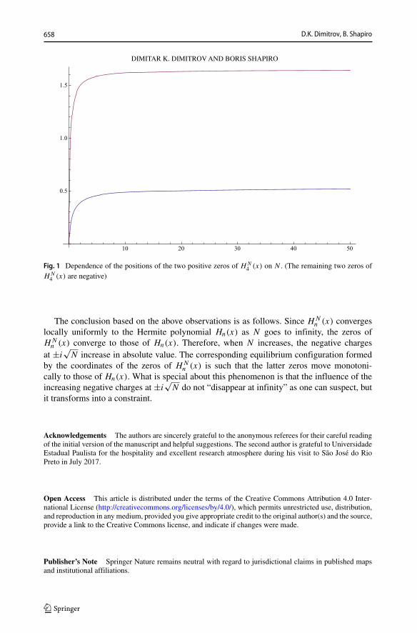
• When N → +∞, the force of attraction of the fixed negative charges decreases becausethey move away from the real line, but at the same time their strength increases in sucha way that the location of each movable charge has a limit, see Fig. 1.
Electrostatic Problems with a Rational Constraint and Degenerate... 657
10 20 30 40 50
0.5
1.0
1.5
DIMITAR K. DIMITROV AND BORIS SHAPIRO
Fig. 1 Dependence of the positions of the two positive zeros of HN4 (x) on N . (The remaining two zeros of
HN4 (x) are negative)
The conclusion based on the above observations is as follows. Since HNn (x) converges
locally uniformly to the Hermite polynomial Hn(x) as N goes to infinity, the zeros ofHN
n (x) converge to those of Hn(x). Therefore, when N increases, the negative chargesat ±i
√N increase in absolute value. The corresponding equilibrium configuration formed
by the coordinates of the zeros of HNn (x) is such that the latter zeros move monotoni-
cally to those of Hn(x). What is special about this phenomenon is that the influence of theincreasing negative charges at ±i
√N do not “disappear at infinity” as one can suspect, but
it transforms into a constraint.
Acknowledgements The authors are sincerely grateful to the anonymous referees for their careful readingof the initial version of the manuscript and helpful suggestions. The second author is grateful to UniversidadeEstadual Paulista for the hospitality and excellent research atmosphere during his visit to Sao Jose do RioPreto in July 2017.
Open Access This article is distributed under the terms of the Creative Commons Attribution 4.0 Inter-national License (http://creativecommons.org/licenses/by/4.0/), which permits unrestricted use, distribution,and reproduction in any medium, provided you give appropriate credit to the original author(s) and the source,provide a link to the Creative Commons license, and indicate if changes were made.
Publisher’s Note Springer Nature remains neutral with regard to jurisdictional claims in published mapsand institutional affiliations.
D.K. Dimitrov, B. Shapiro658

References
1. Dimitrov, D.K.: A late report on interlacing of zeros of polynomials. In: Nikolov, G., Uluchev, R. (eds.)Constructive Theory of Functions, Sozopol 2010: in Memory of Borislav Bojanov, pp. 69–79. MarinDrinov Academic Publishing House, Sofia (2012)
2. Gawronski, W., Van Assche, W.: Strong asymptotics for relativistic Hermite polynomials, RockyMountain. J. Math. 33, 489–524 (2003)
3. Gunning, R.C., Hugo, R.: Analytic Functions of Several Complex Variables, Prentice-Hall Series inModern Analysis, pp. xiv+317. Prentice-Hall, Englewood Cliffs (1965)
4. Heine, E.: Handbuch der Kugelfunctionen. G Reimer Verlag, Berlin (1878). vol. 1, pp. 472–4795. Klein, F.: Uber die Nullstellen von den Polynomen und den Potenzreihen, Gottingen, pp. 211–218 (1894)6. Korevaar, J., Wiegerinck, J.: Several complex variables, version November 18, 2011, p. 260. https://staff.
fnwi.uva.nl/j.j.o.o.wiegerinck/edu/scv/scv1.pdf7. Lundengrd, K., Osterberg, J., Silvestrov, S.: Optimization of the determinant of the Vandermonde matrix
and related matrices. AIP Conference Proceedings 1637(1), 627–636 (2014)8. Lundengrd, K., Osterberg, J., Silvestrov, S.: Extreme points of the Vandermonde determinant on the
sphere and some limits involving the generalized Vandermonde determinant, arXiv:1312.61939. Lundengrd, K.: Generalized Vandermonde matrices and determinants in electromagnetic compatibility.
Malardalen University Press Licentiate Theses 253, 157 (2017)10. Polya, G.: Sur un theoreme de Stieltjes. C. R. Acad. Sci. Paris 155, 767–769 (1912)11. Shapiro, B.: Algebro-geometric aspects of Heine-Stieltjes theory. J. London Math. Soc. 83, 36–56 (2011)12. Stieltjes, T.J.: Sur certains polynomes qui verifient une equation differentielle lineaire du second ordre
et sur la theorie des fonctions de Lame. Acta Math. 6(1), 321–326 (1885)13. Szego, G.: Orthogonal Polynomials, 4th edn., Amer. Math. Soc. Coll. Publ., vol. 23, Providence RI
(1975)14. Varchenko, A.: Multidimensional Hypergeometric Functions the Representation Theory of Lie Algebras
and Quantum Groups. World Scientific Publishing Company15. Varchenko, A.: Critical points of the product of powers of linear functions and families of bases of
singular vectors. Compos. Math. 97, 385–401 (1995)16. Van Vleck, E.B.: On the polynomials of Stieltjes. Bull. Amer. Math. Soc. 4, 426–438 (1898)
Electrostatic Problems with a Rational Constraint and Degenerate... 659