Embed Size (px)
Citation preview
Universidade Federal de Santa Catarina
Programa de Pos-Graduacao em Engenharia Mecanica
Analise Cinematica
Hierarquica de Robos
Manipuladores
Tese de Doutoramento submetida a
Universidade Federal de Santa Catarina
como requisito parcial a obtencao do grau de
Doutor em Engenharia Mecanica
por
Daniel Martins
Florianopolis, Fevereiro de 2002

A minha esposa
Andreia
e as minhas filhas
Barbara Augusta e Maria Eugenia. . .

AgradecimentosAo Prof Raul Guenther, pela amizade e pela paciencia em me guiar
pela ardua tarefa da escrita da tese.
Aos colegas Henrique Simas, Alexandre Campos, Emerson Raposo,
Julio Feller Golin, Waldoir Valentim Gomes Junior, Lucas Weih-
mann, Carlos Henrique Santos
Ao Prof Jose Carlos Zanini, que me iniciou nas lides da teoria de
mecanismos e maquinas.
Aos meus alunos e orientados, que muito me serviram de inspi-
racao e motivacao para a execucao deste trabalho.
AcknowledgementsTo Dr Craig Tischler and Prof Kenneth Hunt ( in memoriam) for
their patience in revealing me the inner secrets of screw theory and
geometry.
To Dr David Downing and Dr Stuart Lucas for a pleasant company
and very helpful comments when I was in Melbourne and even after
my short visit to the University of Melbourne.

Contents
List of Figures p. ii
List of Tables p. iii
Abstract p. iv
Abstract p. v
1 Introduction p. 1
1.1 Singularities . . . . . . . . . . . . . . . . . . . . . . . . . . . . . p. 2
1.2 Purposes of the method . . . . . . . . . . . . . . . . . . . . . . p. 3
1.3 Hierarchical analysis: a simple example . . . . . . . . . . . . . . p. 4
1.4 Extensions to the method . . . . . . . . . . . . . . . . . . . . . p. 7
1.5 Overview of the work . . . . . . . . . . . . . . . . . . . . . . . . p. 8
2 Hierarchical Kinematic Analysis p. 10
2.1 Permutation matrices . . . . . . . . . . . . . . . . . . . . . . . . p. 10
2.2 Digraph Analysis of Jacobian Matrices . . . . . . . . . . . . . . p. 12
2.2.1 Graph definitions . . . . . . . . . . . . . . . . . . . . . . p. 13
2.2.2 Strong components of a digraph . . . . . . . . . . . . . . p. 15

Contents ii
2.2.3 Related matrices R, S, T . . . . . . . . . . . . . . . . . . p. 18
2.3 Hierarchical Jacobian reordering . . . . . . . . . . . . . . . . . . p. 23
3 Jacobian Matrices and Screws p. 25
3.1 Sparsity of the Jacobian matrix . . . . . . . . . . . . . . . . . . p. 25
3.2 Denavit-Hartenberg method . . . . . . . . . . . . . . . . . . . . p. 26
3.3 Velocities along a serial chain . . . . . . . . . . . . . . . . . . . p. 27
3.4 Screw-based Jacobian matrix . . . . . . . . . . . . . . . . . . . p. 31
3.5 Screw dependence of the joint variables . . . . . . . . . . . . . . p. 34
3.6 Line permutations of the Jacobian matrix . . . . . . . . . . . . p. 39
4 Serial Robots p. 41
4.1 Hierarchical analysis of a Puma robot . . . . . . . . . . . . . . . p. 41
4.2 Hierarchical canonical form . . . . . . . . . . . . . . . . . . . . p. 45
4.3 Jacobian Inversion . . . . . . . . . . . . . . . . . . . . . . . . . p. 46
4.4 Hierarchical analysis . . . . . . . . . . . . . . . . . . . . . . . . p. 47
4.5 Other advantages . . . . . . . . . . . . . . . . . . . . . . . . . . p. 49
5 Redundant Robots p. 51
5.1 Introduction to redundant robots . . . . . . . . . . . . . . . . . p. 51
5.2 Redundancy resolution . . . . . . . . . . . . . . . . . . . . . . . p. 53
5.3 Extended Jacobian method . . . . . . . . . . . . . . . . . . . . p. 54
5.3.1 Comparison with generalised inverse methods . . . . . . p. 56
Contents iii
5.3.2 Hierarchical kinematic analysis using extended Jacobian
method . . . . . . . . . . . . . . . . . . . . . . . . . . . p. 58
5.4 Globally constrained Jacobian method . . . . . . . . . . . . . . p. 58
5.4.1 The simplest choice ~n = ei . . . . . . . . . . . . . . . . . p. 60
5.4.2 Algorithmic singularities . . . . . . . . . . . . . . . . . . p. 61
5.4.3 Hierarchical kinematic analysis using globally constrained
Jacobian method . . . . . . . . . . . . . . . . . . . . . . p. 62
5.5 Hierarchy of the singularities of the Roboturb robot . . . . . . . p. 62
5.6 Final comments . . . . . . . . . . . . . . . . . . . . . . . . . . . p. 68
6 Parallel Robots p. 69
6.1 Overview of the chapter . . . . . . . . . . . . . . . . . . . . . . p. 70
6.2 Requisites of the hierarchical kinematic analysis . . . . . . . . . p. 70
6.3 Parallel robots: an introduction . . . . . . . . . . . . . . . . . . p. 71
6.3.1 Stewart-Gough platforms . . . . . . . . . . . . . . . . . . p. 73
6.4 Kinematic problem of parallel robots . . . . . . . . . . . . . . . p. 74
6.5 Kirchhoff-Davies laws and parallel robots . . . . . . . . . . . . . p. 75
6.6 Hierarchical kinematic analysis of parallel robots . . . . . . . . . p. 79
6.7 Permutation of the system . . . . . . . . . . . . . . . . . . . . . p. 81
6.7.1 Actuators at joints A, F , G . . . . . . . . . . . . . . . . p. 82
6.7.2 Actuators at joints D, E, F . . . . . . . . . . . . . . . . p. 83
6.7.3 Actuators at joints A, F , E . . . . . . . . . . . . . . . . p. 84
6.8 Assur groups . . . . . . . . . . . . . . . . . . . . . . . . . . . . p. 86
6.9 Conclusions about parallel robots . . . . . . . . . . . . . . . . . p. 88
Contents iv
7 Conclusions p. 90
7.1 Perspectives and further work . . . . . . . . . . . . . . . . . . . p. 91
Appendix A -- Screw Theory p. 94
A.1 Kinematics and Statics of a rigid body . . . . . . . . . . . . . . p. 94
A.1.1 Line vectors and free vectors . . . . . . . . . . . . . . . . p. 95
A.1.2 Statics . . . . . . . . . . . . . . . . . . . . . . . . . . . . p. 96
A.1.3 Kinematics . . . . . . . . . . . . . . . . . . . . . . . . . p. 97
A.2 Screw Theory . . . . . . . . . . . . . . . . . . . . . . . . . . . . p. 98
A.2.1 Twists × Wrenches . . . . . . . . . . . . . . . . . . . . . p. 99
A.2.1.1 Twists . . . . . . . . . . . . . . . . . . . . . . . p. 99
A.2.1.2 Wrenches . . . . . . . . . . . . . . . . . . . . . p. 100
A.2.2 Screws . . . . . . . . . . . . . . . . . . . . . . . . . . . . p. 100
A.2.3 Plucker coordinates . . . . . . . . . . . . . . . . . . . . . p. 104
A.2.3.1 Plucker line coordinates . . . . . . . . . . . . . p. 104
A.2.3.2 Plucker screw coordinates . . . . . . . . . . . . p. 105
A.2.4 Normalised screws . . . . . . . . . . . . . . . . . . . . . p. 107
A.2.5 Ray order × Axis order . . . . . . . . . . . . . . . . . . p. 110
A.2.6 Virtual Work . . . . . . . . . . . . . . . . . . . . . . . . p. 113
A.3 Screw Coordinate Transformation . . . . . . . . . . . . . . . . . p. 117
A.3.1 Ray-axis screw coordinate transformation . . . . . . . . p. 118
A.3.2 Translation of axes . . . . . . . . . . . . . . . . . . . . . p. 118
A.3.3 Rotation of axes . . . . . . . . . . . . . . . . . . . . . . p. 120

Contents v
Appendix B -- Chasles’ and Poinsot’s lines p. 123
B.1 Screw independence on representation . . . . . . . . . . . . . . . p. 123
B.1.1 Pitch invariance . . . . . . . . . . . . . . . . . . . . . . . p. 124
B.1.2 Axis invariance . . . . . . . . . . . . . . . . . . . . . . . p. 124
B.2 A slightly different approach . . . . . . . . . . . . . . . . . . . . p. 125
Appendix C -- Matrix powers p. 127
Appendix D -- Numerical Inverse Jacobian p. 130
Appendix E -- Kirchhoff-Davies circuit law p. 133
E.1 Adaptation of the Kirchhoff laws to Kinematics . . . . . . . . . p. 133
E.2 Coupling graph of a kinematic chain . . . . . . . . . . . . . . . p. 134
E.3 Movement graph of a kinematic chain . . . . . . . . . . . . . . . p. 137
E.4 Kirchhoff-Davies circuit law . . . . . . . . . . . . . . . . . . . . p. 139
References p. 143

List of Figures
1 The SCARA robot. . . . . . . . . . . . . . . . . . . . . . . . . . p. 5
2 Directed graph (digraph) . . . . . . . . . . . . . . . . . . . . . . p. 13
3 Matrix, incidency matrix and digraph . . . . . . . . . . . . . . . p. 13
4 Digraph of the Scara Jacobian according to eq. (1.2) . . . . . . . p. 16
5 Condensation of the digraph related to the Scara Jacobian . . . p. 17
6 Manipulator with all joints frozen . . . . . . . . . . . . . . . . . p. 28
7 manipulator with all but the last joint frozen . . . . . . . . . . . p. 29
8 manipulator with all but the penultimate joint frozen . . . . . . p. 30
9 Representation of a normalised screw . . . . . . . . . . . . . . . p. 32
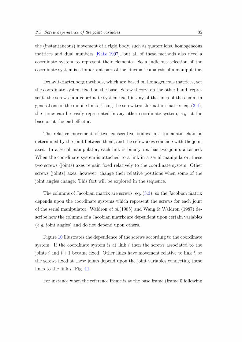
10 Sequence of links in a serial kinematic chain with the coordinate
system fixed at link i. . . . . . . . . . . . . . . . . . . . . . . . . p. 36
11 Sequence of links in a serial kinematic chain with the coordinate
system fixed at link i making explicit the screw dependence of
the joint variables qi. Mobile links are filled in black. . . . . . . p. 36
12 The Puma robot analyzed in this work. The screw $5, which is
not explicitly designated on the Figure is on the joint axis 5 in
the middle of the spherical wrist. . . . . . . . . . . . . . . . . . p. 42
13 Side view (xz-plane) of the Puma. . . . . . . . . . . . . . . . . . p. 42
14 Frontal view (yz-plane ) of the Puma highlighting the spherical
wrist. . . . . . . . . . . . . . . . . . . . . . . . . . . . . . . . . . p. 43

List of Figures vii
15 A sketch of the Puma robot with all joint variables at initial po-
sition.The coordinate system highlighted has origin at the wrist
centre and is fixed on link 3. . . . . . . . . . . . . . . . . . . . . p. 44
16 Condensation digraph of a Puma robot Jacobian based on the
system given by eq. (4.3). Vertex A of the condensation digraph
is the source of the digraph and vertex E is the sink of the
digraph. A singularity at the vertex D divides the condensation
digraph in two parts: one affected by the singularity and the
other free from singularity effects . . . . . . . . . . . . . . . . . p. 49
17 Comparison of the constraints of the globally constraint Jaco-
bian method and the classical extended Jacobian method seen
from a 2-dimensional projection of the R7 space. Scalars ri are
projections of the values of r in eq. (5.8). Negative values for r,
and correspondingly ri are also possible. . . . . . . . . . . . . . p. 60
18 The Roboturb manipulator . . . . . . . . . . . . . . . . . . . . . p. 63
19 Coordinate system chosen to the Roboturb robot . . . . . . . . p. 64
20 The planar Stewart platform 3RRR being actuated at joints A,
F , G. The greater triangle 1 is attached to the base (fixed link or
fixed platform) and the triangle 4 is the moving link or moving
platform . . . . . . . . . . . . . . . . . . . . . . . . . . . . . . . p. 75
21 Details of the the dimensions (lengths and angles) as well as of
the chosen coordinate system to represent the mechanism 3RRR
in the xy-plane . . . . . . . . . . . . . . . . . . . . . . . . . . . p. 76
22 Coupling graph of mechanism 3RRR. . . . . . . . . . . . . . . . p. 76
23 Chords and circuits of the movement graph GM for the mecha-
nism 3RRR. This graph coincides with the coupling graph GC
as there is no kinematic pairs with f > 1. . . . . . . . . . . . . . p. 77
24 Mechanism 3RRR actuated at joints A, F , G . . . . . . . . . . p. 82

List of Figures viii
25 Mechanism 3RRR actuated at joints D, E, F . . . . . . . . . . p. 83
26 Mechanism 3RRR actuated at joints A, F , E . . . . . . . . . . p. 85
27 Pair of first order Assur groups derived from mechanism 3RRR
actuated at joints D, E, F shown in Fig. 25. The pair of As-
sur groups, in this case two dyads, can be solved in any order,
e.g. Assur group 1 can be solved after or before Assur group 2. . p. 88
28 Pair of first order Assur groups derived from mechanism 3RRR
actuated at joints A, F , E shown in Fig. 26. Notice that this
Figure as a whole is non-minimal Assur group, but it can be
split up into two minimal Assur groups, in this case two dyads
which must be solved in order: Assur group 1 always before
Assur group 2. . . . . . . . . . . . . . . . . . . . . . . . . . . . . p. 89
29 Second order Assur group derived from the mechanism 3RRR
actuated at joints A, F , G shown in Fig. 24. Notice that this
Figure as a whole is a minimal Assur group, so it cannot be split
up into smaller Assur groups. . . . . . . . . . . . . . . . . . . . p. 89
30 Line-vectors a) Forces b) Angular velocities. . . . . . . . . . . . p. 96
31 Chasles’ line and Poinsot’s line. . . . . . . . . . . . . . . . . . . p. 101
32 Twist represented by a screw (plus a dimensional magnitude).
The velocity of a point A is given by vA = τ + ω × ~OA . . . . . p. 111
33 Wrench represented by a screw (plus a dimensional magnitude).
The summation of couples at a point A is given by MA = C +
F × ~OA . . . . . . . . . . . . . . . . . . . . . . . . . . . . . . . p. 111
34 A wrench $w acting on a twist $t. . . . . . . . . . . . . . . . . . p. 114
35 Virtual work of a wrench acting on a twist. . . . . . . . . . . . . p. 115
36 Details of the point dependent vector decomposition relative to
the wrench and to the twist. . . . . . . . . . . . . . . . . . . . . p. 115
List of Figures ix
37 Mechanism 3RRR in the xy-plane . . . . . . . . . . . . . . . . . p. 135
38 Graph of mechanism 3RRR. . . . . . . . . . . . . . . . . . . . . p. 135
39 Chords and circuits of the graph GC for the mechanism 3RRR . p. 137
40 Chords and circuits of the graph GM for the mechanism 3RRR p. 138

List of Tables
1 Normalised screws $ , pitches h and magnitudes qi for rotative
and prismatic pairs . . . . . . . . . . . . . . . . . . . . . . . . . p. 32
2 Comparison between Statics and Kinematics. All variables are
represented in SI units and are taken relative to a generic point Pp. 110
3 Combination of factors to generate the virtual work . . . . . . . p. 116
Abstract
Devido a sua estrutura cinematica, os robos manipuladores seriais apresentamsingularidades, que sao definidas como as configuracoes onde a mobilidade domanipulador e reduzida. Matematicamente estas configuracoes correspondemaquelas onde a matriz Jacobiana perde posto. As singularidades introduzemproblemas nas operacoes do robo que precisam ser evitadas.
Normalmente isto e feito detectando-se a priori a configuracao singular e en-tao desviando-se dela. Os metodos usuais para o evitamento de singularidadesconsideram implicitamente todas as singularidades igualmente desastrosas a cin-ematica do robo. Este fato torna mais difıcil o estabelecimento de uma estrategiapara o desvio de singularidades.
Esta tese introduz um metodo novo de analise, designado de analise cin-ematica hierarquica, que e baseado no fato de que as singularidades cinematicasdo robo nao sao igualmente importantes para o comportamento do manipulador.As singularidades sao classificadas de acordo com a sua influencia na cinematicainversa do robo. Alem disso, este metodo fornece um algoritmo recursivo pararesolver mais rapidamente, e com maior exatidao, o problema inverso da cin-ematica de robos seriais. O metodo, que e baseado em uma interpretacao graficada matriz Jacobiana, e sumarizado em um algoritmo.
Para ilustrar sua utilidade, este algoritmo e aplicado a um robo Puma. Osresultados sao interpretados e, mesmo neste exemplo classico, alguns fatos novospodem ser extraıdos usando a analise cinematica hierarquica.
Nos ultimos capıtulos o metodo e estendido a dois casos mais gerais: robos re-dundantes e robos paralelos. A solucao de robos redundantes requereu uma novaformulacao para resolver a redundancia. A solucao de robo paralelos nao utilizadiretamente a matriz Jacobiana mas sim uma matriz auxiliar de solucao. O pro-cedimento requereu o uso das leis de Kirchhoff-Davies e os resultados apresentamuma conexao direta com o conceito classico de grupos de Assur.

Abstract
Due to their kinematic structure, serial robot manipulators present singulari-ties, which are defined as the configurations where the mobility of the manipulatoris reduced. Mathematically, these singular configurations are those where the Ja-cobian matrix of the robot drops rank. Singularities introduce problems in therobot operations that need to be avoided.
Usually this is done by detecting the singular configuration and then deviat-ing from them. The usual methods for singularity avoidance implicitly considerall singularities equally disastrous to the robot kinematics; therefore, the estab-lishment of an strategy to deviate from the singularities becomes more difficult.
This paper introduces a new analysis method, designated as the hierarchicalkinematic analysis, which is based on the fact that the robot kinematic singulari-ties are not equally important to the behaviour of the manipulator. Singularitiesare ranked according to the their influence on the robot inverse kinematics. More-over, this method provides a recursive algorithm to solve faster, and with moreaccuracy, the inverse kinematics problem of serial robots. The method, which isbased on a graphical interpretation of the Jacobian matrix, is summarized in aalgorithm.
To illustrates its usefulness, this algorithm is applied to a Puma robot. Theresults are interpretated and, even in this classical example, some new facts canbe extracted by using the hierarchical kinematic analysis.
In the last chapters, the method is extended to two more general cases: re-dundant robots and parallel robots. The redundant robot solution demanded fora different form of solving the redundancy. The parallel robot solution does notuse the Jacobian matrix directly, but an intermediary matrix. The procedure wasbased on the Kirchhoff-Davies laws, and the results have a close connection withthe classical concept of Assur groups.

1
1 Introduction
Mas eu que falo, humilde, baxo e rudo,
De vos nao conhecido nem sonhado?
Da boca dos pequenos sei, contudo,
Que o louvor sai as vezes acabado.
Tem me falta na vida honesto estudo,
Com longa experiencia misturado,
Nem engenho, que aqui vereis presente,
Cousas que juntas se acham raramente.
Luıs de Camoes – Os Lusıadas, Canto Decimo – 154
As a rule, the end-effector of a serial robot is programmed to follow a set of
desired positions and orientations in the Cartesian space. Positions and orien-
tations first derivatives (velocities) are often imposed as extra conditions on the
path tracking. Transforming these motion specifications into the corresponding
joint space motions requires solving the inverse kinematics problem, which is the
determination of the joint variables related to a given end-effector position and
orientation.
The inverse kinematics, at differential level, can be represented by a linear
system
J(q)q = x (1.1)
where vector q comprises the joint variables, e.g. rotation angles if all joint are
rotative. Vector q of joint velocities, the time derivative of vector q, is related
1.1 Singularities 2
to vector x of end-effector velocities, specified as the desired velocities, by the
Jacobian matrix J(q). The matrix J(q), also designated simply by Jacobian,
must be inverted to solve eq. (1.1).
The inverse of the Jacobian, J−1, may be used to solve the inverse kinematic
problem even when only positions and orientations (and not their derivatives) are
specified. Inverting the Jacobian avoids solving the inverse kinematic problem
in closed form, as closed-form solutions are available only to simple kinematic
structures [Sciavicco e Siciliano 1996].
So, in general, the inverse kinematic problem solution demands the inversion
of the Jacobian matrix, a computationally expensive route [Lucas, Tischler e
Samuel 2000], particularly when this inversion has to be done online [Zomaya,
Smith e Olariu 1999].
1.1 Singularities
The Jacobian is a function of the robot geometrical parameters and, nor-
mally, of the configuration q; therefore, it may drop rank at some configurations.
Those configurations q where J(q) is rank deficient are termed kinematic singu-
larities. Kinematic singularities, in serial robots, represent configurations where
the mobility of the structure is reduced, i.e. an arbitrary movement to the end-
effector cannot be imposed. Furthermore, small velocities in the Cartesian space
may require large velocities in the joint space when the manipulator reaches the
neighbourhood of a singularity.
The problems introduced by singularities need to be avoided, e.g. by deviating
from those singular configurations. Avoiding singularities is normally done off-
line, i.e. first these configurations are to be a priori detected and then, when the
robot is moving and before the singularity is reached, they are deviated from. In
the worst case, when a singularity is reached, another strategy has to be employed
to escape from the singularity within feasible joint velocities.
1.2 Purposes of the method 3
A matrix J drops rank when e.g. two columns (or rows) are linearly dependent
each other. In this case det J = 0. The matrix J also drops rank when a line
(row or column) is null; therefore, det J = 0 is also satisfied in this case. So, an
equation like det J = 0 cannot be used to distinguish among these quite different
cases. The use of this equation to detect singularities is possibly originated by the
widely spread idea that all singularities are equally disastrous to the manipulator
kinematics, as each singularity leads det J to zero “equally”.
Standard algorithms, see a review at [Nakamura e Hanafusa 1986], detect the
proximity of a singularity but do not specify, or simply do not care about, which
particular singularity is being reached. Such algorithms, most of them based on
the determinant or the singular values of the Jacobian, turn the differences among
singularities hardly discernible.
1.2 Purposes of the method
By introducing a new analysis method, we intend to achieve three main pur-
poses. The first one is to provide a recursive algorithm to solve faster, and
with more accuracy, the inverse kinematics problem of serial robots based on a
preliminary Jacobian manipulation. The second purpose is to outline that all
singularities are not equally important to the behaviour of the manipulator. Fi-
nally, the third purpose is to explicitly determine the set of variables affected by
and responsible for each singularity.
We designate this new method as the hierarchical kinematic analysis, which is
a method based entirely on the structure of the Jacobian and on the reduction of
the Jacobian matrix to its finest block-triangular form. Sometimes this reduction
may be done easily by inspection, as described in section 1.3 for the SCARA
robot, but this only applies to quite simple manipulators. Moreover, the block-
triangular form obtained by inspection cannot be ensured to be the finest one,
e.g. another rearrangement, not so obvious, may yield smaller diagonal blocks. In
other words, a systematic method which leads a sparse matrix to its finest block-

1.3 Hierarchical analysis: a simple example 4
triangular form is needed. Such method, based on directed graphs, is described
in chapters 2-4.
The Jacobian matrix sparsity is crucial to all methods which represent matri-
ces by graphs [Pissanetsky 1984]. Chapter 3 describes how screw theory can be
employed to enhance the sparsity of the Jacobian matrix before using the method
described in chapter 2
A complete hierarchical kinematic analysis is performed on a Puma robot in
chapter 4.
1.3 Hierarchical analysis: a simple example
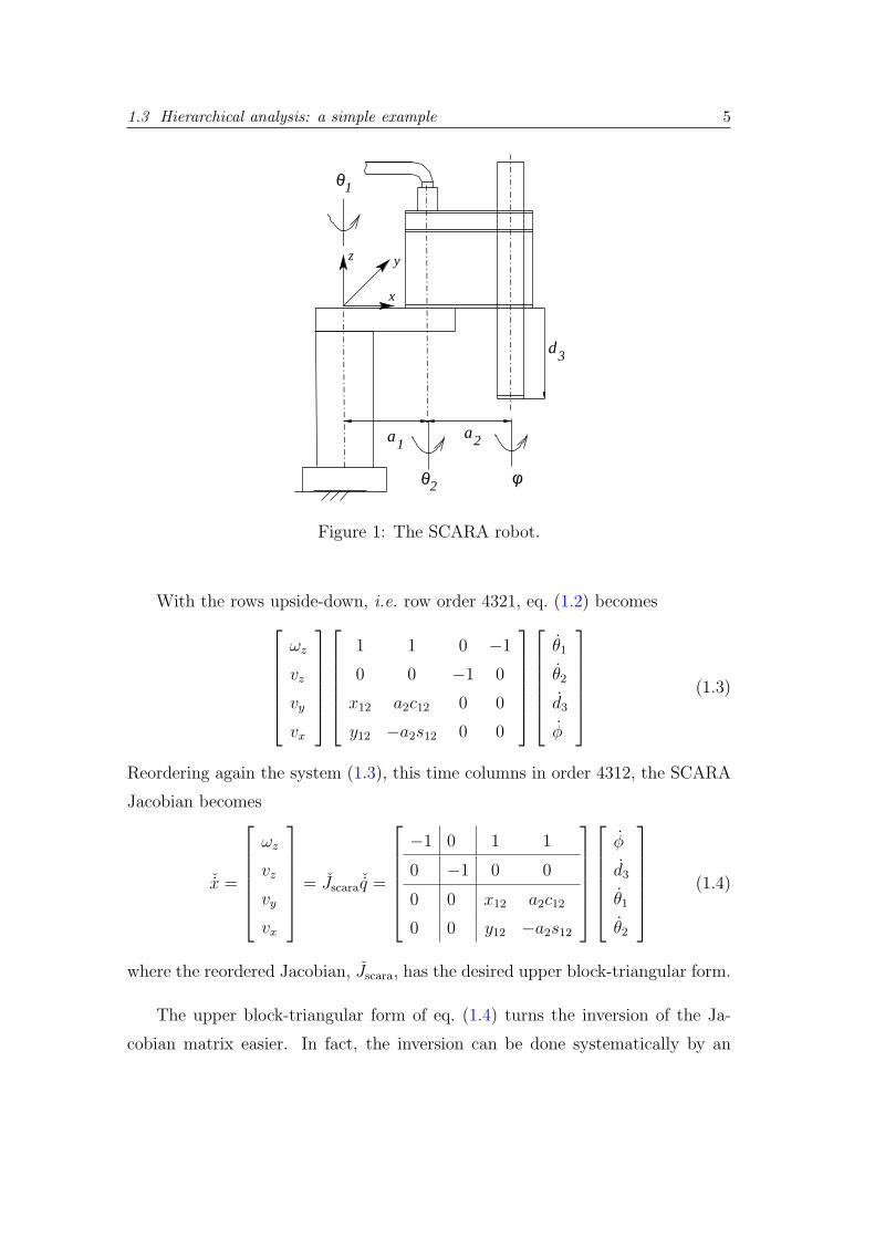
The usefulness of the proposed hierarchical analysis will be outlined by a sim-
ple example; therefore, we intentionally chose a SCARA robot with four degrees
of freedom (θ1, θ2, d3, φ) along three axes, Fig. 1. The Jacobian matrix of this
robot, relating the velocity vector in the Cartesian space, xscara = [vx vy vz ωz]T ,
and the joint velocity vector, qscara = [θ1 θ2 d3 φ]T , may be described by [Spong
e Vidyasagar 1989]
x =
vx
vy
vz
ωz
=
y12 −a2s12 0 0
x12 a2c12 0 0
0 0 −1 0
1 1 0 −1
θ1
θ2
d3
φ
= Jq (1.2)
where ai is the length of link i; y12 = −a1s1 + a2s12; x12 = −a1c1 + a2c12; θ1, θ2, φ
are the rate of rotation about the revolute joints; d3 is the rate of the linear
displacement of the prismatic joint; and si, ci, s12, c12 are the commonly accepted
short notation for sin θi, cos θi, sin(θ1 + θ2), cos(θ1 + θ2), respectively.
The hierarchical analysis is based on reordering the Jacobian into an upper
block-triangular form. The finest reordering scheme for this simple example al-
most reveals itself and it can be obtained following two steps: first changing the
rows upside-down, and then reordering the columns.
1.3 Hierarchical analysis: a simple example 5
yz
x
d3
a1a2
1θ
φ2θ
Figure 1: The SCARA robot.
With the rows upside-down, i.e. row order 4321, eq. (1.2) becomesωz
vz
vy
vx
1 1 0 −1
0 0 −1 0
x12 a2c12 0 0
y12 −a2s12 0 0
θ1
θ2
d3
φ
(1.3)
Reordering again the system (1.3), this time columns in order 4312, the SCARA
Jacobian becomes
ˇx =
ωz
vz
vy
vx
= Jscaraˇq =
−1 0 1 1
0 −1 0 0
0 0 x12 a2c12
0 0 y12 −a2s12
φ
d3
θ1
θ2
(1.4)
where the reordered Jacobian, Jscara, has the desired upper block-triangular form.
The upper block-triangular form of eq. (1.4) turns the inversion of the Ja-
cobian matrix easier. In fact, the inversion can be done systematically by an
1.3 Hierarchical analysis: a simple example 6
(almost) back-substitution process. From bottom to top the whole system (1.2)
becomes a chained series of subsystems to be solved in order. For example, the
solution of the inverse kinematic problem is obtained by the following steps[θ1
θ2
]=
[x12 a2c12
y12 −a2s12
]−1 [vy
vx
](1.5)
d3 = −vz (1.6)
φ = −1 · ωz + [1 1]
[θ1
θ2
](1.7)
where eq. (1.7) is solved only after obtaining the values of eq. (1.5). Equa-
tion (1.5), in turn, requires the inversion of a simple 2 × 2 system. Briefly, this
process uses less memory, induces fewer errors, and is easier to compute.
The block-triangular form, eq. (1.4), allows establishing a hierarchy of vari-
ables, because the relationship among variables becomes apparent. The block-
triangular form itself describes how the variables affect one another and, maybe
more importantly, which group of variables do not affect some other group of
variables.
For instance, d3 exclusively depends upon vz and vice-versa. Similarly, θ1, θ2
only depend upon vy, vx and vice-versa. Moreover φ = φ(ωz; θ1, θ2) and ωz =
ωz(φ; vy, vx).
Furthermore, the upper block-triangular form of eq. (1.4) introduces other
advantages when compared to the original form (1.2). Some of these advantages
appears even in this simple example, like:
• the hierarchy of diagonal blocks highlights a hierarchy of singularities. Un-
fortunately, this fact cannot be inferred from eq. (1.4) as the first diagonal
blocks are scalar and do not vary with the movement of the robot, so there
is only one singularity for the SCARA robot. This problem will be discussed
for a Puma robot in chapter 4.
• the pivoting process in a numerical LU decomposition [Golub e Loan 1983]

1.4 Extensions to the method 7
of an upper block-triangular matrix is almost done without aggregating
errors to the solution. Solving directly eq. (1.4) is better than solving
eq. (1.2) even when the decomposition, like eqs. (1.5)- (1.7), is not used.
• the determinant is easier to obtain. From eq. (1.4) we observe that the
determinant is explicitly constrained to the determinant of the 2×2 diagonal
block at the bottom of system:
[x12 a2c12
y12 −a2s12
].
1.4 Extensions to the method
Above, we described the hierarchical kinematic analysis from a nonredundant
serial robot point of view. However, this method can be extended to other types
of manipulators, namely redundant and parallel robots. These extensions requires
some adaptation and will be described in chapter 5, for redundant robots, and
chapter 6, for parallel robots.
Redundant robots, chapter 5, have non-square Jacobian matrices, turning
difficult the inversion and the use of the hierarchical kinematic analysis. One
approach to the redundancy resolution is the extended Jacobian method, i.e. the
addition of an extra line to “square” the Jacobian; the hierarchical kinematic
analysis could be, in principle, applied to this extended Jacobian.
The problem in the classical extended Jacobian methods is the selection of
the extra row. These classical methods rely on general minimisation criteria and
these criteria normally couple all the variables that were not originally coupled.
To overcome this difficulty we propose an alternative variant of the extended
Jacobian method, called globally constrained Jacobian method. This variant has
advantages over the extended Jacobian method in the setting of the constraints
and in the singularity avoidance.
Parallel robots, chapter 6, have an even higher complexity in their kinemat-
ics. Normally the inverse kinematics problem for parallel robots is considerably
simpler than the direct kinematics problem. The closure of the kinematic chain

1.5 Overview of the work 8
impose a first, and quite important, problem: the determination of the parame-
ters of all joints.
Differently from serial and redundant robots, not all joints in a parallel robot
are actuated. Some of the joints in the closed kinematic chain of a parallel robot
are passive, and their parameters (position, velocity, acceleration, . . . ) are depen-
dent upon the actuated joints parameters. The calculation of these parameters
at differential level (velocities) can be posed as a linear system obtained by the
Kirchhoff-Davies laws, see section 6.5 at page 75 and appendix E at page 133.
The solution of this linear system may be improved by the hierarchical kine-
matic analysis. As a collateral effect, we notice a close relationship between the
block-triangular form of the rearranged system and the intrinsic kinematic struc-
ture of the mechanism, in this case represented by Assur groups, section 6.8 at
page 86.
1.5 Overview of the work
Chapter 2, gives the graph theoretical basis of the hierarchical kinematic
analysis. This chapter relates matrices and graphs and discusses how the sparsity
of a matrix can be represented by its associated graph. The main result of the
chapter is the Algorithm 1 at page 22 that leads a matrix to its finest block-
triangular form by independent permutations of rows and columns.
Chapter 3 shows the relationship between the sparsity of the Jacobian and
the geometry of the robot. It discusses also the choice of the “best” coordinate
system, i.e. the system which leads to a sparser Jacobian.
Chapter 4 details the hierarchical kinematic analysis to serial robots. The
hierarchical kinematic analysis is applied to the Puma robot, and even in this
classical example some new results appear.
Chapter 5 extends the hierarchical kinematic analysis to redundant robots. It
also discusses some methods to the redundancy resolution, in special the extended
1.5 Overview of the work 9
Jacobian method. In this chapter a variant of the extended Jacobian method is
proposed: the globally constrained Jacobian method. The results are applied to
the Roboturb manipulator. The Roboturb manipulator is a redundant welding
manipulator, designed and built at the Universidade Federal de Santa Catarina in
a joint venture with the LacTec institute (Curitiba-Brazil), for repairing eroded
turbine blades.
Chapter 6 extends the hierarchical kinematic analysis to parallel robots. This
chapter also discusses some prerequisites of the hierarchical kinematic analysis
which were trivially satisfied by the serial and redundant formulations. The
proposal of the chapter uses the Kirchhoff-Davies laws to obtain the parallel
robot kinematics. The results are applied to a planar version of the Stewart-
Gough platform, the 3RRR manipulator.
Appendix A develops screw theory from a dual vector approach. Contrarily to
most texts in screw theory, this chapter describes some fundamentals of rigid body
motion with no pre-requisite. The duality statics-kinematics is also presented.
The text do not use advanced geometrical concepts such as projective geometry
and Plucker’s conoid (cylindroid). They are mentioned only when necessary. No
previous knowledge of these topics is required.
Appendix B demonstrates the theorems of Chasles and Poinsot, cite and used
in appendix A, in two different ways. This appendix also details some properties,
as the screw representation invariance, section B.1.
Appendix C discusses the matrix powers in the context of graph analysis. It
completes the demonstration of some steps before the Algorithm 1.
Appendix D provides an alternative way of obtaining the structure of the
inverse matrix used in Algorithm 1. The structure of the inverse matrix is used
without applying symbolic inversion.
Appendix E details the Kirchhoff-Davies laws used in the parallel robot kine-
matic analysis.

10
2 Hierarchical KinematicAnalysis
2.1 Permutation matrices
The tougher step in the whole process described in section 1.3 is to obtain
the order of rows and columns that reduce the Jacobian to an upper block-
triangular form. The row order 4321 and column order 4312 are selected from
the 4! × 4! = 576 possible independent permutations of rows and columns. For
the Scara robot these permutations can be found by inspection or, at most, with
a little number of trials.
An equivalent way to look at the search of a row order, like 4321 from eq. (1.2)
to eq. (1.3), and a column order, like 4321 from eq. (1.3) to eq. (1.4), is to look for
their corresponding permutation matrices. Hence, the problem can be restated
as: to find a pair of permutation matrices, Pr for rows and Pc for columns, that
reorder the system described in eq. (1.2).
A permutation matrix is a matrix whose rows are formed by versors ei where
the only non-null element is the i-th element which has value 1. For instance,
in the example above, the process to obtain ˇx from x can be described by the

2.1 Permutation matrices 11
following procedure
ˇx =
0 0 0 1
0 0 1 0
0 1 0 0
1 0 0 0
x =
· · · ~e4 · · ·· · · ~e3 · · ·· · · ~e2 · · ·· · · ~e1 · · ·
x = Prx (2.1)
Permutation matrices have interesting properties. An important property is that
permutation matrices P are orthonormal matrices and so PP T = P T P = I.
Using this property and eq. (2.1) we can obtain eq. (1.4) from eq. (1.2) by a
different route. Defining ˇx , Prx, the rearranged Cartesian velocities vector, and
ˇq , Pcq, the rearranged joint velocities vector, we obtain
ˇx = J ˇq (2.2)
where J = PrJP Tc is the reordered Jacobian matrix. The permutation matrix
Pr corresponds to the row permutation of the J and the permutation matrix Pc
corresponds to the column permutation of the J .
With this new definitions, the problem of reordering the Jacobian matrix
can now be restated as: find a pair of permutation matrices, Pr for rows and
Pc for columns, such that the reordered Jacobian matrix J = PrJP Tc has the
finest upper block-triangular form. The finest upper block-triangular form of
the Jacobian matrix will be designated as the hierarchical canonical form of the
Jacobian.
Another question that arises is whether the obtained block-triangular form
can be reordered to a finer upper block-triangular form i.e. with smaller diagonal
blocks. Eq. (1.4) has only one 2× 2 diagonal block and, again by inspection, we
can notice that this block cannot be split into two one-dimensional blocks by any
permutation. Any attempt to split this block will unavoidably create another
2× 2 diagonal block or destroy the block-triangular form.
The hierarchical canonical form for more complex robot architectures, such as
those with 6 degrees of freedom, will hardly expose itself so easily as the block-

2.2 Digraph Analysis of Jacobian Matrices 12
triangular form of the Scara robot. So there is a need of a systematic search
method for this form. Next sections will describe an algorithmic method, based
on directed graphs, which obtains the hierarchical canonical form of the Jacobian
matrix.
2.2 Digraph Analysis of Jacobian Matrices
Above we were acquainted with the necessity of a systematic method to de-
rive the block-triangular form of a sparse matrix. Several methods exist to re-
duce a matrix to a block-triangular form. Most of these methods are based on
graphs [Pissanetsky 1984], yet there are some works which propose a matroid
approach [Murota 2000]. Depending of the type of the matrix and computational
requirements a certain type of graph is required.
Pissanetsky (1984) makes a good review of the graph-based methods from
the computational point of view. If the matrix is symmetrical the most natural
representation is based on non-directed graphs; however, if the matrix is general,
i.e. not symmetrical, two options appears: bipartite graphs and directed graphs.
Bipartite graphs implicitly apply rows and columns permutations to the matrix,
while directed graphs are restricted to the simultaneous row and column permu-
tation. On the other hand, we believe that directed graphs expresses more clearly
the interdependency of the variables and, therefore, clarify the flow of variables
from one step to another. In this work, we obtain both independent permuta-
tions on the Jacobian matrix and, at the same time, these rearrangements are
applied to the inverse Jacobian, by introducing the kinematic structure matrix
in section 2.3.
Now, we start describing a method based on directed graphs; the main con-
cepts will be summarized in this and in the following sections. More detail on this
topic can be found on [Murota 2000] [Harary, Norman e Cartwright 1965] [Rein-
schke 1988] and references therein.
2.2 Digraph Analysis of Jacobian Matrices 13
2.2.1 Graph definitions
A graph G is a structure which consist of vertices or nodes and links. The
links can be orientated, arcs, or non-orientated,edges A vertex is a point in the
graph and an edge is a line connecting two vertices. A subgraph of a graph G is
a graph whose vertices and links are vertices and links of G.
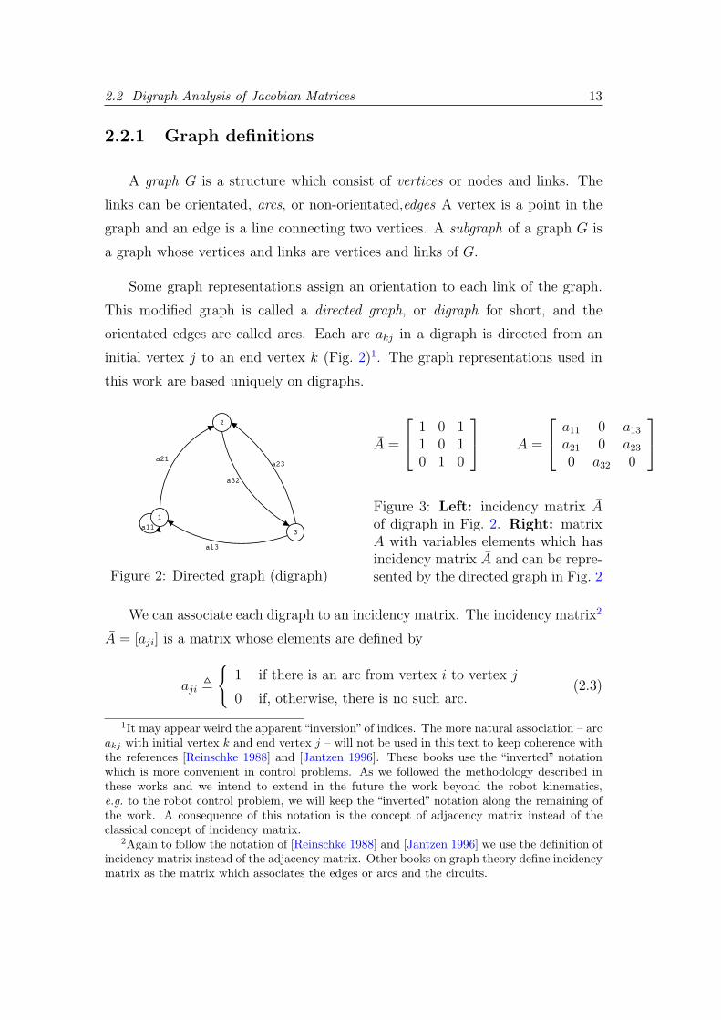
Some graph representations assign an orientation to each link of the graph.
This modified graph is called a directed graph, or digraph for short, and the
orientated edges are called arcs. Each arc akj in a digraph is directed from an
initial vertex j to an end vertex k (Fig. 2)1. The graph representations used in
this work are based uniquely on digraphs.
a21
a13
a23
a32
a11
2
1
3
Figure 2: Directed graph (digraph)
A =
1 0 11 0 10 1 0
A =
a11 0 a13
a21 0 a23
0 a32 0
Figure 3: Left: incidency matrix Aof digraph in Fig. 2. Right: matrixA with variables elements which hasincidency matrix A and can be repre-sented by the directed graph in Fig. 2
We can associate each digraph to an incidency matrix. The incidency matrix2
A = [aji] is a matrix whose elements are defined by
aji ,
{1 if there is an arc from vertex i to vertex j
0 if, otherwise, there is no such arc.(2.3)
1It may appear weird the apparent “inversion”of indices. The more natural association – arcakj with initial vertex k and end vertex j – will not be used in this text to keep coherence withthe references [Reinschke 1988] and [Jantzen 1996]. These books use the “inverted” notationwhich is more convenient in control problems. As we followed the methodology described inthese works and we intend to extend in the future the work beyond the robot kinematics,e.g. to the robot control problem, we will keep the “inverted” notation along the remaining ofthe work. A consequence of this notation is the concept of adjacency matrix instead of theclassical concept of incidency matrix.
2Again to follow the notation of [Reinschke 1988] and [Jantzen 1996] we use the definition ofincidency matrix instead of the adjacency matrix. Other books on graph theory define incidencymatrix as the matrix which associates the edges or arcs and the circuits.
2.2 Digraph Analysis of Jacobian Matrices 14
The incidency matrix is a Boolean matrix in a sense that their elements, only 0’s
or 1’s, satisfy Boolean arithmetics operations. Boolean arithmetics share most of
the properties of the real numbers. The only difference between Boolean addition
and real addition is 1+1 = 1. At first glance, it seems to be an awkward result but,
in fact, it is derived from the logical equation 1∨1 = 1 or 1 = 1. Boolean matrices
are here designated by Roman capital letters with an overbar like A, R, T , . . . A
graph related to an incidency matrix A is designated by G(A).
A specific labelling of vertices in G(A) is irrelevant to the properties of the
graph itself. Relabelling the vertices has no impact on the digraph intrinsic
properties but produces a simultaneous row and column permutation on the cor-
responding incidency matrix. Such permutations can be used to reorder the
associated matrix. A good reordering can lead the matrix to a block triangular
form using the concept of strong components of a digraph.
Up to now, we have derived a matrix from a digraph. Our problem, however,
requires the inverse procedure i.e. to know how to derive a graph from a matrix.
For this reason, we need to be acquaint with the concept of structure of a sparse
matrix.
Real matrices, e.g. Jacobian matrices, are often sparse matrices. The struc-
ture of a sparse matrix, also called structure matrix, is the relative position in
the matrix of the null and non-null elements. The structure matrix can be rep-
resented by a Boolean matrix simply by changing the non-null elements by the
number 1 and keeping the null elements as 0.
This Boolean matrix can be considered as the incidency matrix of an asso-
ciated graph and, with some abuse of terminology, the incidency matrix of the
real matrix. Figure 2 shows a simple digraph whose incidency matrix is shown
in Fig. 3 on the left. The real matrix, Fig. 3 on the right, is a matrix whose
associated digraph is shown in Fig. 2.
Vertices of an associated digraph can be related to the input and output
variables of the linear system represented by eq. (1.1) i.e. to the velocities at
2.2 Digraph Analysis of Jacobian Matrices 15
Cartesian and joint space. This association will be described in more detail
in section 2.3. Up to now, it is sufficient to state that diagonal blocks of the
hierarchical canonical form of the Jacobian, as obtained in eq. (1.4), have intrinsic
relationship to the role that these associated variables play on the sequentially
organized inversion of the Jacobian e.g. eqs. (1.5)- (1.7).
There is an intrinsic connection between the diagonal blocks and the strong
components of the digraph. The relative positions of these diagonal blocks have
also a correspondence with the partial order among these diagonal blocks. These
concepts will be explained below.
2.2.2 Strong components of a digraph
The main concept used in this work related to directed graphs is the concept
of strong components [Harary, Norman e Cartwright 1965]. This concept will be
derived here as an extension of the concept of reachability.
To reach the concept of reachability we have to define some preliminary graph
concepts. A path ia a sequence of arcs {e1, e2, . . .} where the initial vertex of the
succeeding arc (ei+1) is the final vertex of the preceding arc (ei). The length of a
path is the number of arcs in the path. A path comprising a single arc has unit
length. Let two vertices i and j be part of a same directed graph G. Vertex j is
said reachable from vertex i, symbolically i ⇀ j, if exists a (directed) path from
vertex i to vertex j.
Two vertices i and j are strongly connected if exists a path from vertex i to
vertex j as well as a path from vertex j to vertex i. Two strongly connected
vertices i and j will be designated by the symbol i j like 2 3 in Fig. 2. By
definition a vertex is always strongly connected to itself (i i). The concept of
strongly connected vertices can be extended from a pair of vertices to a generic
set of vertices. A subgraph is a strong component of the digraph or a strongly
connected set of vertices if every two vertices are strongly connected.
2.2 Digraph Analysis of Jacobian Matrices 16
zv
3
z
xv
1 yv
2
. .
. . .
. .
.
d
w
q
q
φ
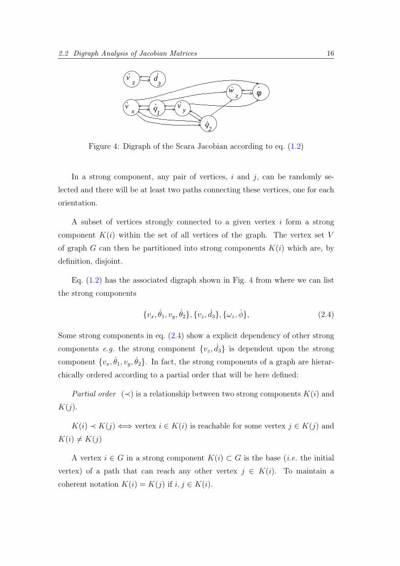
Figure 4: Digraph of the Scara Jacobian according to eq. (1.2)
In a strong component, any pair of vertices, i and j, can be randomly se-
lected and there will be at least two paths connecting these vertices, one for each
orientation.
A subset of vertices strongly connected to a given vertex i form a strong
component K(i) within the set of all vertices of the graph. The vertex set V
of graph G can then be partitioned into strong components K(i) which are, by
definition, disjoint.
Eq. (1.2) has the associated digraph shown in Fig. 4 from where we can list
the strong components
{vx, θ1, vy, θ2}, {vz, d3}, {ωz, φ}, (2.4)
Some strong components in eq. (2.4) show a explicit dependency of other strong
components e.g. the strong component {vz, d3} is dependent upon the strong
component {vx, θ1, vy, θ2}. In fact, the strong components of a graph are hierar-
chically ordered according to a partial order that will be here defined:
Partial order (≺) is a relationship between two strong components K(i) and
K(j).
K(i) ≺ K(j) ⇐⇒ vertex i ∈ K(i) is reachable for some vertex j ∈ K(j) and
K(i) 6= K(j)
A vertex i ∈ G in a strong component K(i) ⊂ G is the base (i.e. the initial
vertex) of a path that can reach any other vertex j ∈ K(i). To maintain a
coherent notation K(i) = K(j) if i, j ∈ K(i).

2.2 Digraph Analysis of Jacobian Matrices 17
zv
3
z
xv
1 yv
2
.
.
.
.
d
w φ
q
q
Figure 5: Condensation of the digraph related to the Scara Jacobian
Partial order leads to the concept of condensation of a digraph. The con-
densation of a digraph is a digraph whose vertices are the strong components of
the digraph. The condensation of a digraph is more precisely a tree because a
loop or cycle in the condensation imply that the strong components were not well
determined.
A tree, like Fig. 5, has sources and sinks [Harary, Norman e Cartwright
1965] which corresponds to the beginning and the end of the tree. Sources are
the variables which correspond to a vertex in the condensation digraph with no
output arcs. Sinks, on the other hand, are variables which correspond to a vertex
in the condensation digraph with no input arcs.
The source variables have priority on the solution of eq. (1.1). Variables
θ1, θ2; vy, vx are the sources of the Scara. Joint velocities and end-effector veloci-
ties are separated by a semi-colon “;” as they play different roles on the forward
and inverse kinematics. Sources must be solved first in the inverse kinematic
problem.
The sink variables are those which have complete dependency of the remaining
variables. In the inverse kinematic problem they are solved at the final steps of
the algorithm. Variables φ and ωz are the sinks of the Scara.
An isolated vertex in the condensation digraph is at same time a source and
a sink. Vertex B in Fig. 5 is isolated and points out that variables vz and d3 are
completely independent from the remaining variables. These isolated vertices can
be solved at any time because they have no influence on the remaining variables
2.2 Digraph Analysis of Jacobian Matrices 18
of the system.
2.2.3 Related matrices R, S, T
In the prior sections, we have shown the relationship among the incidency ma-
trix, the associated digraph and the block-triangular form. The block-triangular
form is derived from the strong components of the associated digraph. There are
several methods to extract the strong components of a digraph and they can be
divided into two groups: those directly based on a computational structure which
represents the graph itself and those based on the incidency matrix representation
of the digraph.
The first group covers methods which rely on linked chains or object-oriented
analysis [Orwant, Hietaniemi e Macdonald 1999]. Other methods of the first
group are those based on a different graph theoretical basis for the representation
of the system, like methods based on bipartite graphs [Murota 1987] [Harary
1967]. Both approaches require some expertise of the programmer as well as the
availability of the software tools.
While methods based on the structure of the graph itself have some advan-
tages over the incidency matrix methods they lack some didactic appeal. More-
over their use impose strong prerequisites both at conceptual level and at pro-
gramming level. Such requisites can puzzle researchers not directly concerned
with some subtleties of graph theory as, for instance, roboticists. On the other
hand, robot researchers are normally well trained in the use of simulation soft-
wares, specially those matrix orientated, such as Matlab [Corke 1996]. This fact
is improved by the existence of free matrix-based simulation softwares such as
Octave [Eaton 1996], which is the simulation software used to obtain all results
in this paper.
For this reason we take a route that converges to the matrix-based Algo-
rithm 1. This algorithm is based on the work of Reinschke [Reinschke 1988] and
it is entirely based on manipulations of the incidency matrix. The remaining of

2.2 Digraph Analysis of Jacobian Matrices 19
this section intends to clarify these manipulations and to interpret the interme-
diary matrices generated by the Algorithm 1.
First, we define the reachability matrix R that maps the “inter-accessibility”
of vertices. The matrix R = [rij] can be defined element by element, as
rij =
{1 if a path leads from vertex j to vertex i
0 if, otherwise, vertex i cannot be reached starting from vertex j
(2.5)
Harary et al.(1965) discuss how to obtain the reachability matrix from the
incidency matrix based on some properties of the product of Boolean matrices and
power of Boolean matrices in terms of their corresponding associated digraphs.
A discussion about the properties of the power of incidency matrices is presented
at the Appendix C. This discussion derives the reachability matrix from the
incidency matrix using the following summation
R =n−1∑k=0
Ak (2.6)
As matrix A is Boolean, eq. (2.6) has multiplication replaced by the Boolean and
(∧) and sum replaced by the Boolean or (∨). The same definitions are valid for
other Boolean matrices like S and T described below.
If the reachability matrix is full then a path starting at vertex i and ending
at a different vertex j can always be found. The interdependency of all vari-
ables is complete. In matricial terms this means that there is no simultaneous
permutation of rows and columns that lead this matrix to a block-triangular form.
A full reachability matrix is a signal of stop. Nothing more can be done to
reduce the initial incidency matrix to an upper block-triangular form. A full
incidency matrix, by eq. (2.6), implies in a full reachability matrix. However the
converse is not true: a full reachability matrix can be obtained from a sparse
incidency matrix e.g. the digraph in Fig. 2 is fully reachable and the reachability
matrix derived from the sparse matrix A in Fig. 3 is full.
2.2 Digraph Analysis of Jacobian Matrices 20
When the reachability matrix has some zeros a block-triangular form can
always be reached [Harary, Norman e Cartwright 1965]. In this case, two other
Boolean matrices, S and T , help us to reduce the original matrix A to an upper
block-triangular form.
The symmetrical structure Boolean matrix S shows the strong component
K(i) associated with each vertex i. Matrix S comes directly from the reachability
matrix R by
S , R ∧ RT (2.7)
i.e. each element sij from S satisfy
sij = rij · rji (2.8)
The matrix S maps all strong components of vertices in a directed graph. A
column j of S (which corresponds to vertex j) has “connections” with all vertices
i whose elements sij 6= 0, i = 1, n. Strong components K(j) are formed by
all vertices i such that sij 6= 0. By definition, two strong components with the
same number of variables are either disjoint or congruent i.e. are the same strong
component.
The symmetrical structure matrix S = [sij] can be alternatively defined by
sij =
{1 if vertices i and j are strongly connected.
0 otherwise.(2.9)
The asymmetrical structure Boolean matrix T differentiates strong components
one another.
T , R ∧v RT
(2.10)
where the operator v is the Boolean not applied to all elements of the Boolean
matrix. The matrix v R is simply a change 0 1 of all elements of the original
Boolean matrix R.
In other words
tij = rij· v rji (2.11)
2.2 Digraph Analysis of Jacobian Matrices 21
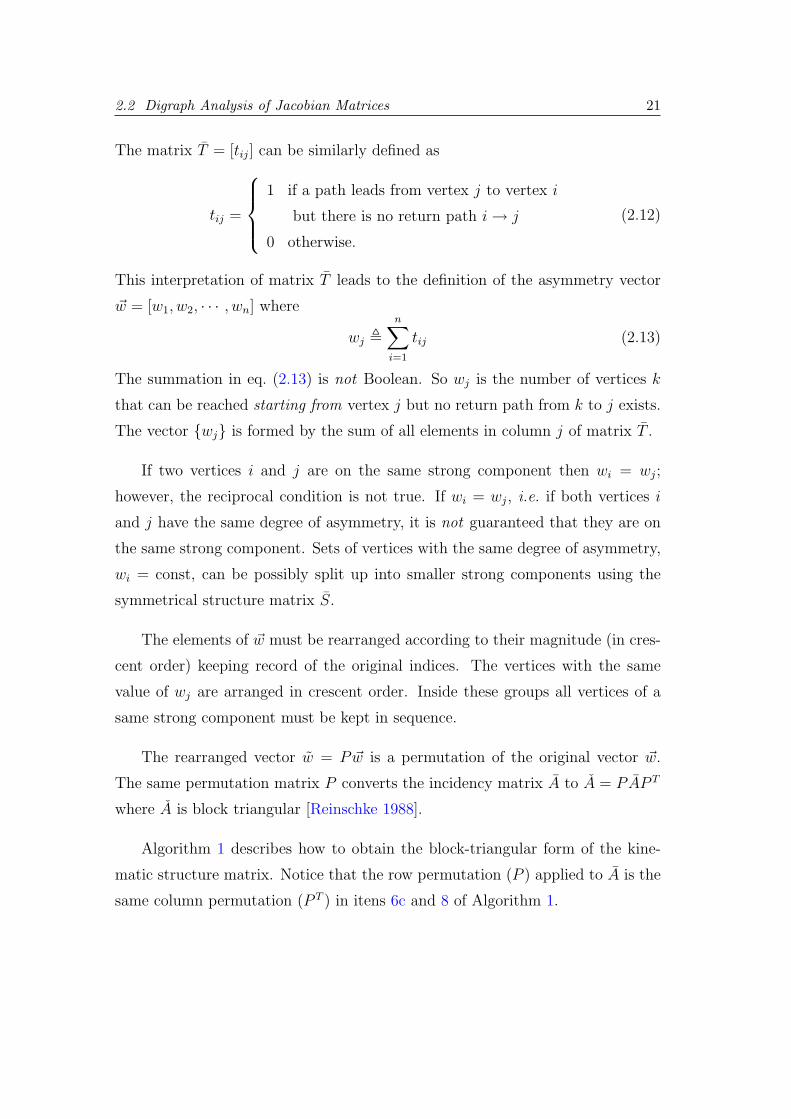
The matrix T = [tij] can be similarly defined as
tij =
1 if a path leads from vertex j to vertex i
but there is no return path i → j
0 otherwise.
(2.12)
This interpretation of matrix T leads to the definition of the asymmetry vector
~w = [w1, w2, · · · , wn] where
wj ,n∑
i=1
tij (2.13)
The summation in eq. (2.13) is not Boolean. So wj is the number of vertices k
that can be reached starting from vertex j but no return path from k to j exists.
The vector {wj} is formed by the sum of all elements in column j of matrix T .
If two vertices i and j are on the same strong component then wi = wj;
however, the reciprocal condition is not true. If wi = wj, i.e. if both vertices i
and j have the same degree of asymmetry, it is not guaranteed that they are on
the same strong component. Sets of vertices with the same degree of asymmetry,
wi = const, can be possibly split up into smaller strong components using the
symmetrical structure matrix S.
The elements of ~w must be rearranged according to their magnitude (in cres-
cent order) keeping record of the original indices. The vertices with the same
value of wj are arranged in crescent order. Inside these groups all vertices of a
same strong component must be kept in sequence.
The rearranged vector w = P ~w is a permutation of the original vector ~w.
The same permutation matrix P converts the incidency matrix A to A = PAP T
where A is block triangular [Reinschke 1988].
Algorithm 1 describes how to obtain the block-triangular form of the kine-
matic structure matrix. Notice that the row permutation (P ) applied to A is the
same column permutation (P T ) in itens 6c and 8 of Algorithm 1.

2.2 Digraph Analysis of Jacobian Matrices 22
Algorithm 1: Graph partitioning based on Boolean matrices Reinschke (1988)
• Input data: A
• Output data: reordered matrix A
1. Incidency matrix: A from original matrix A
2. Reachability matrix: R =∑n−1
i−1 Ak
• If R is full, stop. No improvement can be obtained by permutatingrows or columns.
• else, continue.
3. Symmetrical structure matrix: S , R ∧RT
4. Asymmetrical structure matrix: T , R ∧ RT
5. Asymmetry vector: ~w : wj =∑n
i=1 tij
6. Reordering of the asymmetry vector ~w
(a) Reorder the vertices with the same value of wj in crescent order.
(b) Check inside each group of vertices with the same value of wj if thegroup corresponds to more than one strong component. This check-upis done by looking at the corresponding columns of matrix S.
• If these columns are absolutely equal go to item 7.
• Else divide these groups: one for each pattern of the columns ofS.
(c) Reorder these groups internally keeping all vertices of a same strongcomponent in sequence.
7. Find the permutation matrix P that leads {w1, w2, · · · , wn} →{weind1
, weind2, · · · , weindn
} where {eind1 , eind2 , · · · , eindn} is the sequence ofpermuted indices of the original vector.
P =
· · · ~eind1 · · ·· · · ~eind2 · · ·
...· · · ~eindn · · ·
(2.14)
where ~eindjis a row vector corresponding to the j-th row of the identity
matrix In.
8. Reordering of the original matrix A : A = PAP T
2.3 Hierarchical Jacobian reordering 23
2.3 Hierarchical Jacobian reordering
Simultaneous rows and columns permutations are too restrictive to obtain
the block-triangular form of a generally sparse Jacobian matrix. For this reason,
digraph techniques, when directly applied to the Jacobian matrix, have poor
results.
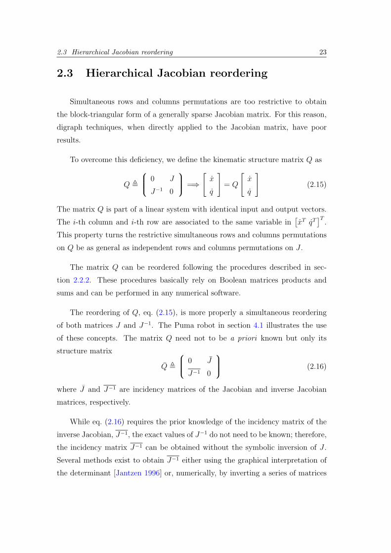
To overcome this deficiency, we define the kinematic structure matrix Q as
Q ,
0 J
J−1 0
=⇒
[x
q
]= Q
[x
q
](2.15)
The matrix Q is part of a linear system with identical input and output vectors.
The i-th column and i-th row are associated to the same variable in[xT qT
]T.
This property turns the restrictive simultaneous rows and columns permutations
on Q be as general as independent rows and columns permutations on J .
The matrix Q can be reordered following the procedures described in sec-
tion 2.2.2. These procedures basically rely on Boolean matrices products and
sums and can be performed in any numerical software.
The reordering of Q, eq. (2.15), is more properly a simultaneous reordering
of both matrices J and J−1. The Puma robot in section 4.1 illustrates the use
of these concepts. The matrix Q need not to be a priori known but only its
structure matrix
Q ,
0 J
J−1 0
(2.16)
where J and J−1 are incidency matrices of the Jacobian and inverse Jacobian
matrices, respectively.
While eq. (2.16) requires the prior knowledge of the incidency matrix of the
inverse Jacobian, J−1, the exact values of J−1 do not need to be known; therefore,
the incidency matrix J−1 can be obtained without the symbolic inversion of J .
Several methods exist to obtain J−1 either using the graphical interpretation of
the determinant [Jantzen 1996] or, numerically, by inverting a series of matrices

2.3 Hierarchical Jacobian reordering 24
whose incidency matrix is J as described in [Martins 2000].
Let Q be the hierarchical canonical form of the kinematic matrix Q, which is
obtained by applying Algorithm 1. Once Q is obtained we have at the same time
the hierarchical canonical form of the Jacobian and also of the inverse Jacobian.
For instance, to obtain the hierarchical canonical form of the Jacobian matrix is
sufficient to drop the lines (rows and columns) which corresponds to the inverse
Jacobian, see the example in section 4.2.

25
3 Jacobian Matrices andScrews
There are two main approaches for obtaining the Jacobian [Tsai 1999]: Denavit-
Hartenberg method and screw-based method. Section 3.2 describes the Denavit-
Hartenberg method. The screw-based method will be described from section 3.4
on.
Section 3.3 is intermediary between both descriptions, and shows how the
velocities of a link in a serial robot depend upon the joint variables. This descrip-
tion is used in section 3.4 to present the concepts of screw theory. Section 3.5
describes how the screws depend upon the joint variables, expanding the results
of section 3.3.
3.1 Sparsity of the Jacobian matrix
The rearrangement of matrices to their block-triangular form using graph
techniques entail sparse matrices [Pissanetsky 1984]. An extreme case is when
the associated digraph of the matrix is strongly connected, section 2.2.2, so any
trial to find a block-triangular form from such matrices is worthless. The opposite
extreme case is when the matrix is upper triangular. In this case, the matrix is
already in the hierarchical canonical form; any permutation of this matrix will
not improve its form.
The Jacobian matrix is not unique for a robot architecture; on the contrary, it
is highly dependent upon the coordinate system. To be profitable, the kinematic

3.2 Denavit-Hartenberg method 26
analysis must explore and enhance the sparsity of the Jacobian matrix as much
as possible before using graph theory.
3.2 Denavit-Hartenberg method
Classical texts in Robotics [Asada e Slotine 1986] [Spong e Vidyasagar 1989]
present the Denavit-Hartenberg method as the method of robot kinematic analy-
sis. Later, other texts [Angeles 1997] [Tsai 1999] present the Denavit-Hartenberg
method in parallel with screw-based analysis method. Although simple and easy
to apply to most of the serial robots, the Denavit-Hartenberg method has some
important drawbacks, e.g. the Jacobian is less sparse and has elements with higher
complexity [Hunt 1987] [Zomaya, Smith e Olariu 1999].
The essence of Denavit-Hartenberg method is the systematic generation of a
series of coordinate systems for the robot. These coordinate systems are based
on geometrical properties of the manipulator as well as the type of the joints of
the manipulator.
Due to its algorithmic features, the Denavit-Hartenberg method permits a
“blind use” of the kinematic principles and alleviates some problems related to
the search of the “best” coordinate system for each manipulator architecture. It
is a handy option for a first contact with a different robot architecture, or when
inverse kinematics efficiency is not a crucial problem. The Denavit-Hartenberg
method also permits a prompt off-line computation of the manipulator model.
The Denavit-Hartenberg method, see e.g. [Spong e Vidyasagar 1989], is es-
sentially an algorithm based on the Denavit-Hartenberg parameters [Denavit e
Hartenberg 1955]. This algorithm obtains, in a systematic way, each one of the
columns of the Jacobian matrix through the multiplication of homogeneous ma-
trices.
These homogeneous matrices relate the movement between the coordinate
systems. Apart from the existence of multiple coordinate systems, the Jacobian

3.3 Velocities along a serial chain 27
matrix is always determined in relation to the first (“0”) coordinate system at the
base. For this reason, the terms which compose the Jacobian matrix are normally
extremely complex.
To minimise the complexity of the Jacobian elements, some authors [Tsai
1999] suggest the use of the“modified”Denavit-Hartenberg method, i.e. the use of
a mobile reference frame to represent the Jacobian matrix. Waldron et al.(1985)
suggests the use of an intermediate link to attach the coordinate system. Al-
though with better form than the original Denavit-Hartenberg Jacobian matrix,
this “modified” Jacobian matrix is still based on the same fixed set of coordinate
systems.
Denavit-Hartenberg coordinate systems are judiciously selected to exploit the
geometrical relations between consecutive links. However, geometrical relations
between non consecutive links, which are not considered by Denavit-Hartenberg
method, can also improve the sparsity of the Jacobian matrix. Screw-based meth-
ods normally take in account both types of relations, so yielding sparser Jacobian
matrices.
In the Denavit-Hartenberg method, most of the coordinate systems are uniquely
determined. This rigid selection of the coordinate systems affects directly the
sparsity of the obtained Jacobian matrix [Hunt 1987]. It is known from the
literature that well chosen coordinate systems improve the sparsity of the Ja-
cobian [Wang e Waldron 1987] [Waldron, Wang e Bolin 1985]. Screw theory
concepts lead to a more suitable choice of the coordinate system [Hunt 1987].
For these reason, we will adopt a screw theory approach to derive the Jacobian
matrix throughout this work.
3.3 Velocities along a serial chain
This section describes the kinematic behaviour of a serial chain. A serial
(kinematic) chain in this context is a series of links connected by joints with one
degree of freedom. Each link in the chain is labelled by a natural number where

3.3 Velocities along a serial chain 28
0 is the base (fixed frame) and n is the end-effector. The objective of this section
is to show how the linear and angular velocities at a generic link i is influenced
by the linear and angular velocities of the previous joints.
Although the example used here is a serial manipulator, the results are quite
general and will be applied to redundant robots, chapter 5, and with some adap-
tation to parallel robots, chapter 6.
Let a serial manipulator in the imminence of being instantaneously displaced.
First, all kinematic pairs in the serial chain are fixed. The whole manipulator
becomes kinematically equivalent to a single rigid body, Fig. 6, satisfying the
rigidity principle discussed in appendix A.1.
���������������� ����������
� ��������� ������
� ��������� ������
� ��������� ������� ��������
� ������
n
n−1
3
2
1
Figure 6: A manipulator with all joints frozen behaving as a rigid body B0−n.
All joints, now instantaneously “frozen”, are considered helical kinematic
pairs. A helical kinematic pair can be visualised as a screw attached to one
link displacing relative to a nut attached to the other link. This screw nut pair
has a pitch h. This pitch can be zero (rotative pair), infinite (prismatic pair)
or any other finite value. In other words, the helical pair is a generalisation of
all kinematic pairs with one degree of freedom that have contact between two
mating surfaces (lower kinematic pairs, see [Hartenberg e Denavit 1964]).

3.3 Velocities along a serial chain 29
The joint n between link n − 1, and the end-effector, link n, is now re-
leased, Fig. 7. An actuator twists this joint with magnitude qn. The “rigid body”
B0−(n−1), a virtual link composed by links 0 to n − 1, remains fixed and, as
expected, is not affected by this input variable qn. The remaining of the ma-
nipulator, namely link n, is still a single rigid body being twisted about the
screw kinematic pair of the joint n, i.e. link n translates and rotates by the sole
imposition of joint n.
If joint n − 1, instead of joint n, is the only joint released a similar result
occurs, Fig. 8. Joint n− 1 connects links n− 2 and n− 1. Two rigid bodies are
divided by joint n− 1, namely B0−(n−2) and B(n−1)−n. Body B0−(n−2), composed
by links 0 to n − 2, is fixed. Body B(n−1)−n, composed by links n − 1 and n,
displaces relatively to body B0−(n−2) i.e. relatively to the base.
���������� ��� ��
����������� ������
��������� �
0−(n−1)��� ��� ��������� B
���������� ��� ��
n−1
2
3
� ��� ��
n
n
1
Figure 7: A manipulator with all joints frozen with the exception of joint nbetween the last and penultimate links. There are two rigid bodies: the end-effector n, and B0−(n−1) composed by the remaining frozen bodies.
If the same reasoning is applied to all joints some conclusions can be extracted
about the translational and angular velocities1 of a link i:
1A discussion of translational and angular velocities in the context of screw theory can be

3.3 Velocities along a serial chain 30
0−(n−2)B
���������������� ���� �����
�������������
(n−1)−n
��� ���� ����� B
� ���������������������n
� ������n−1
����������� ������
� ��������� ����������������� ������
�����! "4 to n−2
2
n−1
n
1
3
Figure 8: A manipulator with all joints frozen with the exception of joint n − 1between links n − 2 and n − 1. There are two rigid bodies: B(n−1)−n composedby links n− 1 and the end-effector n and the remaining frozen bodies B0−(n−2)
• The translational and angular velocities of link i is affected by the twists
imposed on joints 1 to i, i.e. those joints which are between the link i and
the base 0. The remaining joints do not affect velocities of the link i.
• The angular velocity of body i is the vectorial sum of the angular velocities
applied at joints 1 to i.
Let P be a fixed point on the link i. As the velocity of a point is a vector we
also conclude that:
• The linear velocity of a point P at link i is the vectorial sum of the linear
velocities imposed by each of these joints, as if they were acting alone and
independently.
A convenient choice for the point P is the origin of the coordinate system,
this point becomes unambiguously defined whatever link i is chosen. The rigid
found in appendix A and in [Ciblak 1998].

3.4 Screw-based Jacobian matrix 31
body movement of a link is completely determined in a given coordinate system
when
• The angular velocity ω of the link is represented in this coordinate system,
and
• The linear velocity vO of a point which is instantaneously coincident with
the origin O of this coordinate system is also known.
3.4 Screw-based Jacobian matrix
This section shows how to generate the Jacobian matrix using the screw
theory principles. This generation is based on two fundamentals: the linear
properties, and the separation of the magnitude of the screws from their geometric
information. The former was described in the last section, while the latter will
described in the sequence.
Screw theory is based on the physical principles of the rigid kinematics. Rigid
body instantaneous movements can be “carried out by” a screw [Ball 1900]. A
screw is a geometrical element with an axis (line), a pitch and a magnitude in
velocity dimensions (rad/s or m/s). From the conclusion of the last section, the
rigid body instantaneous movement of a link can be described by a pair of vectors
ω and vO, so a screw $i representing the movement of link i can be represented by
the pair $i = (ωi; vO|i). Using screw theory principles [Hunt 1978] [Tsai 1999], we
can extract the geometrical parameters of the screw (axis, pitch and magnitude)
from the representation $i = (ω; vO|i).
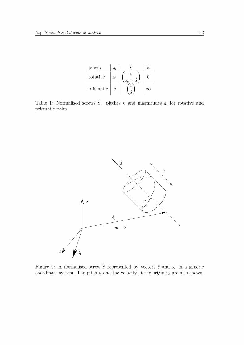
Although the helical pair is the generalisation, in common practice only rota-
tive and prismatic pairs are used. For these cases, Table 1 summarises the values
of axis, pitch and magnitude. There $ is the normalised screw associated with
the joint, s is a unit vector in the direction of the axis, and so is a vector starting
at the origin of the coordinate system and ending in any point along the screw
axis.
3.4 Screw-based Jacobian matrix 32
joint i qi $ h
rotative ω
(s
so × s
)0
prismatic v
(0
s
)∞
Table 1: Normalised screws $ , pitches h and magnitudes qi for rotative andprismatic pairs
so
s
ov
h
y
z
x
Figure 9: A normalised screw $ represented by vectors s and so in a genericcoordinate system. The pitch h and the velocity at the origin vo are also shown.
3.4 Screw-based Jacobian matrix 33
The separation of a screw as a product between the normalised screw and
the magnitude, $i = $iqi allows the determination of the Jacobian matrix almost
directly, sometimes by simple inspection of the robot geometry [Hunt 2000]. The
instantaneous movement of the end-effector $n is the sum of the instantaneous
movements, $i, of the links composing the serial chain.
x = $n =n∑
i=1
$i =n∑
i=1
[JRi
JLi
]qi =
n∑i=1
$iqi (3.1)
where x = $n = [x1, x2, x3, x4, x5, x6]T is represented in an appropriate coordinate
system, JRi= [x1, x2, x3]
T |i, JLi= [x4, x5, x6]
T |i. Each column of the Jacobian is
a normalised screw $i of eq. (3.1) corresponding to the i-th joint. More details
about this topic can be found in [Hunt 1987] and references therein.
Isolating vector q in eq. (3.1) we obtain the system
x = $n = Jq (3.2)
with the Jacobian matrix defined by
J = [$1 $2 $3 · · · $n] (3.3)
Two details about eq. (3.1): vectors JRiand JLi
are consequence of the
linear properties described in section 3.3, and in the Denavit-Hartenberg method
normally the order of the normalised screws is (v; ω) changing the order of the
vectors JRiand JLi
.
Screw theory is more flexible regarding the choice of the coordinate system
than the Denavit-Hartenberg method. In fact, the coordinate system for repre-
senting the screws can be freely chosen and then all joint velocities are represented
in relation to this coordinate system. Furthermore, we can migrate from one co-
ordinate system to another just using one matrix multiplication i.e. the screw
transformation matrix [Hunt 1987]. The screw transformation matrix, here in
ray order and from coordinate system i to coordinate system j, is [Tischler et al.

3.5 Screw dependence of the joint variables 34
2000]
Ti→j ,
[R 0
RS R
].where S ,
0 −xo yo
xo 0 −zo
−yo zo 0
(3.4)
The matrix Ti→j transforms the Jacobian matrix, originally given in a coordinate
system i, into a different coordinate system j i.e. Jj = Ti→jJi. In eq. (3.4)
R = Ri→j is the 3 × 3 rotation matrix from coordinate system i to coordinate
system j [Spong e Vidyasagar 1989], and (xo, yo, zo) are the coordinates of the
origin of the coordinate system j measured in the coordinate system i.
It must be recalled that, the Jacobian matrix, while different in form from
one coordinate system to another, has the same functionality. The screw trans-
formation matrix Ti→j, eq. (3.4), couples, or decouples, the terms that were not
present in other Jacobian representations,e.g. the Denavit-Hartenberg Jacobian
matrix. The main difference is that matrix Ti→j is orthogonal, and then is easily
invertible
T−1i→j =
[RT (RS)T
0 RT
]. (3.5)
where (RS)T = STRT = −STR.
To select a good coordinate system, i.e. a coordinate system which improves
the sparsity of the Jacobian, some geometrical insight is required. Once this
coordinate system is chosen, we apply graph theory techniques to prepare the
Jacobian matrix to the inversion process. The graphical techniques were described
above
To guide the selection of an appropriate coordinate system, the next section
will describe how the screw in a serial chain depend upon of the joint variables.
3.5 Screw dependence of the joint variables
Screws are instantaneous “shots” of the movement of a rigid body, and they
are described in a specific coordinate system. There are several ways to represent
3.5 Screw dependence of the joint variables 35
the (instantaneous) movement of a rigid body, such as quaternions, homogeneous
matrices and dual numbers [Katz 1997], but all of these methods also need a
coordinate system to represent their elements. So a judicious selection of the
coordinate system is a important part of the kinematic analysis of a manipulator.
Denavit-Hartenberg methods, which are based on homogeneous matrices, set
the coordinate system fixed on the base. Screw theory, on the other hand, repre-
sents the screws in a coordinate system fixed in any of the links of the chain, in
general one of the mobile links. Using the screw transformation matrix, eq. (3.4),
the screw can be easily represented in any other coordinate system, e.g. at the
base or at the end-effector.
The relative movement of two consecutive bodies in a kinematic chain is
determined by the joint between them, and the screw axes coincide with the joint
axes. In a serial manipulator, each link is binary i.e. has two joints attached.
When the coordinate system is attached to a link in a serial manipulator, these
two screws (joints) axes remain fixed relatively to the coordinate system. Other
screws (joints) axes, however, change their relative positions when some of the
joint angles change. This fact will be explored in the sequence.
The columns of Jacobian matrix are screws, eq. (3.3), so the Jacobian matrix
depends upon the coordinate systems which represent the screws for each joint
of the serial manipulator. Waldron et al.(1985) and Wang & Waldron (1987) de-
scribe how the columns of a Jacobian matrix are dependent upon certain variables
(e.g. joint angles) and do not depend upon others.
Figure 10 illustrates the dependence of the screws according to the coordinate
system. If the coordinate system is at link i then the screws associated to the
joints i and i + 1 became fixed. Other links have movement relative to link i, so
the screws fixed at these joints depend upon the joint variables connecting these
links to the link i. Fig. 11.
For instance when the reference frame is at the base frame (frame 0 following
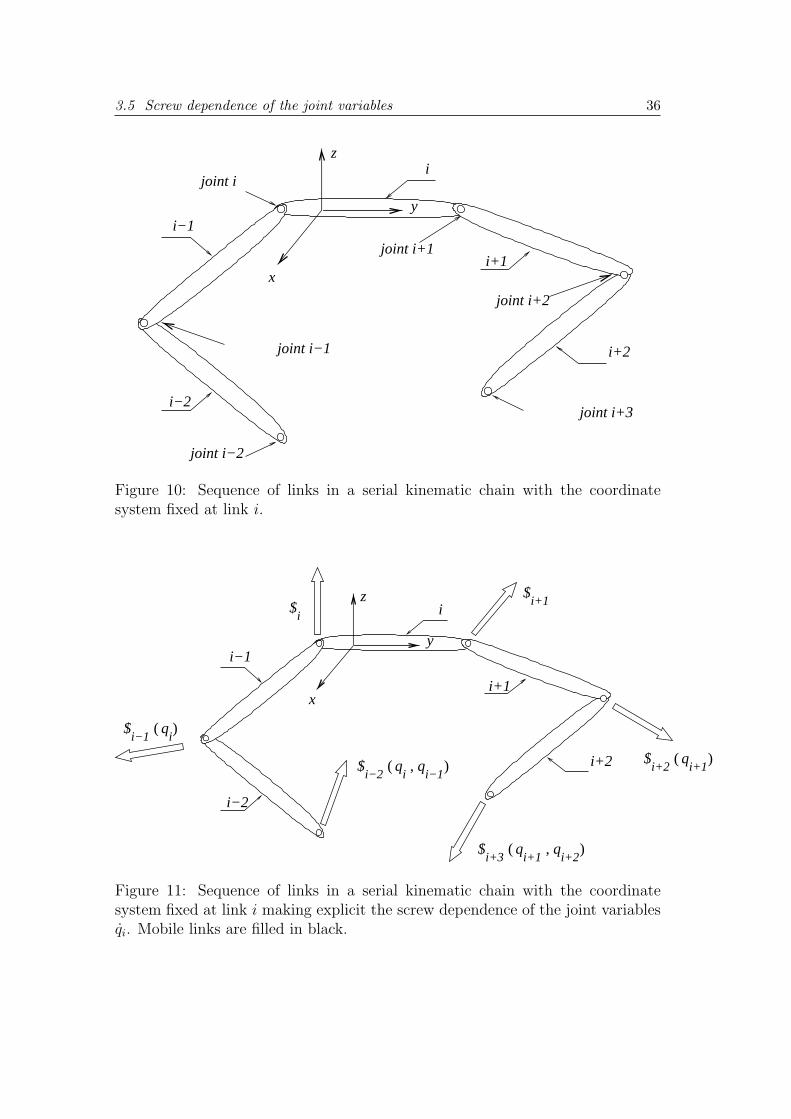
3.5 Screw dependence of the joint variables 36
joint i−2
i−2
i+2
joint i+3
joint i+2
joint i−1
i−1
joint ii
joint i+1i+1
x
y
z
Figure 10: Sequence of links in a serial kinematic chain with the coordinatesystem fixed at link i.
i−2
i
i−1
i+2 $i+2
qi+1
( )
$i−1
qi
( )
$i+1$
i
$i−2
qi
qi−1
( , )
$i+3
qi+1
qi+2
( , )
i+1x
y
z
Figure 11: Sequence of links in a serial kinematic chain with the coordinatesystem fixed at link i making explicit the screw dependence of the joint variablesqi. Mobile links are filled in black.
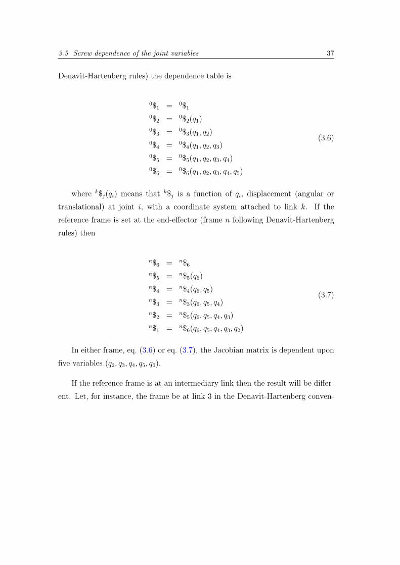
3.5 Screw dependence of the joint variables 37
Denavit-Hartenberg rules) the dependence table is
0$1 = 0$1
0$2 = 0$2(q1)
0$3 = 0$3(q1, q2)
0$4 = 0$4(q1, q2, q3)
0$5 = 0$5(q1, q2, q3, q4)
0$6 = 0$6(q1, q2, q3, q4, q5)
(3.6)
where k$j(qi) means that k$j is a function of qi, displacement (angular or
translational) at joint i, with a coordinate system attached to link k. If the
reference frame is set at the end-effector (frame n following Denavit-Hartenberg
rules) then
n$6 = n$6
n$5 = n$5(q6)
n$4 = n$4(q6, q5)
n$3 = n$3(q6, q5, q4)
n$2 = n$5(q6, q5, q4, q3)
n$1 = n$6(q6, q5, q4, q3, q2)
(3.7)
In either frame, eq. (3.6) or eq. (3.7), the Jacobian matrix is dependent upon
five variables (q2, q3, q4, q5, q6).
If the reference frame is at an intermediary link then the result will be differ-
ent. Let, for instance, the frame be at link 3 in the Denavit-Hartenberg conven-
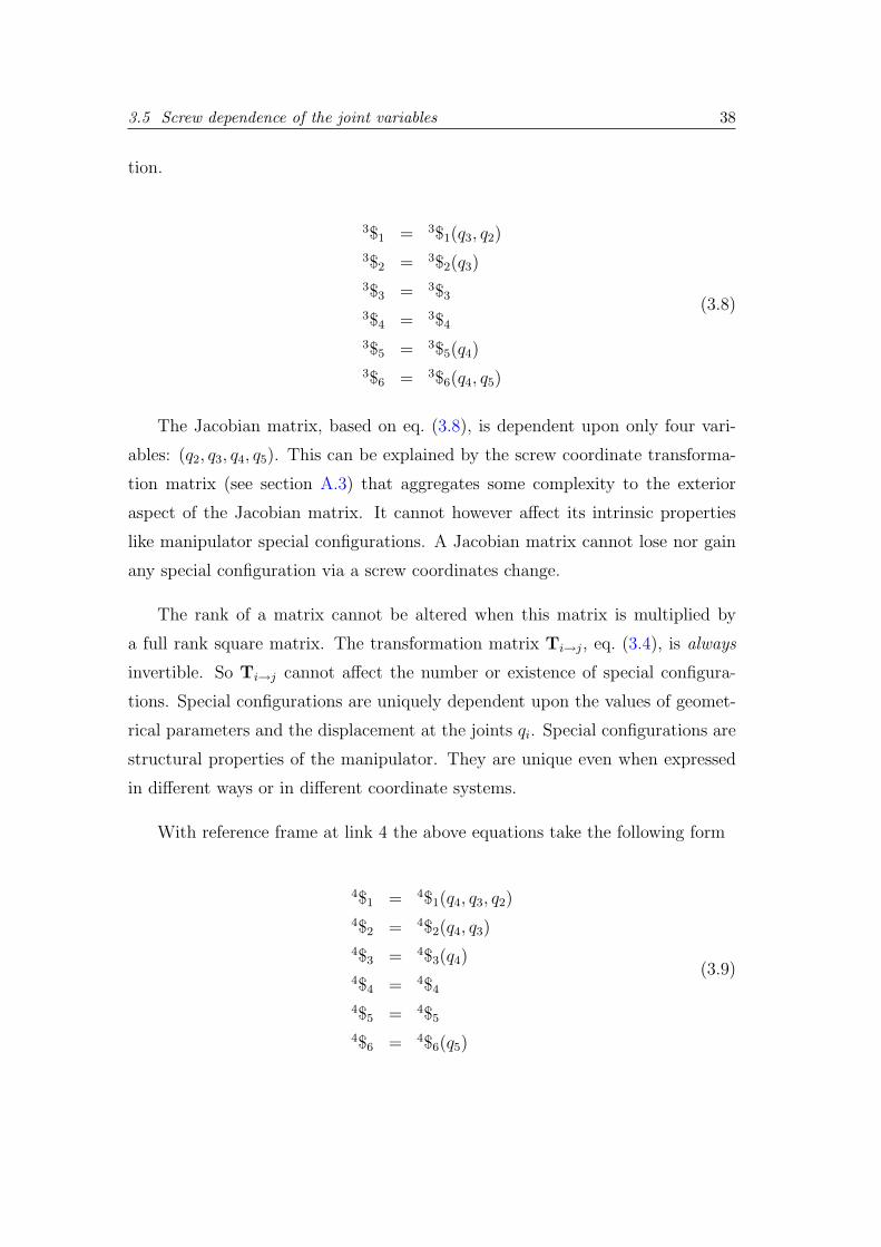
3.5 Screw dependence of the joint variables 38
tion.
3$1 = 3$1(q3, q2)
3$2 = 3$2(q3)
3$3 = 3$3
3$4 = 3$4
3$5 = 3$5(q4)
3$6 = 3$6(q4, q5)
(3.8)
The Jacobian matrix, based on eq. (3.8), is dependent upon only four vari-
ables: (q2, q3, q4, q5). This can be explained by the screw coordinate transforma-
tion matrix (see section A.3) that aggregates some complexity to the exterior
aspect of the Jacobian matrix. It cannot however affect its intrinsic properties
like manipulator special configurations. A Jacobian matrix cannot lose nor gain
any special configuration via a screw coordinates change.
The rank of a matrix cannot be altered when this matrix is multiplied by
a full rank square matrix. The transformation matrix Ti→j, eq. (3.4), is always
invertible. So Ti→j cannot affect the number or existence of special configura-
tions. Special configurations are uniquely dependent upon the values of geomet-
rical parameters and the displacement at the joints qi. Special configurations are
structural properties of the manipulator. They are unique even when expressed
in different ways or in different coordinate systems.
With reference frame at link 4 the above equations take the following form
4$1 = 4$1(q4, q3, q2)
4$2 = 4$2(q4, q3)
4$3 = 4$3(q4)
4$4 = 4$4
4$5 = 4$5
4$6 = 4$6(q5)
(3.9)

3.6 Line permutations of the Jacobian matrix 39
The Jacobian matrix is described by only four variables. Equations like (3.6)-
(3.9) express qualitatively the screw dependency of the columns of the Jacobian
matrix. Eqs. (3.8) and (3.9) show that the initial and final actuator variables have
no effect on the rank of the Jacobian matrix. Eqs. (3.6) and (3.7) have built-in an
“extra” screw transformation (to the base or the end-effector, respectively) that
is always invertible (see eq. (3.4) and comments in appendix A.3).
A specific robot architectures is associated with certain screw subsystems
[Hunt 2000], e.g. the spherical wrist. The knowledge of these subsystems can
improve the choice of a good coordinate system which may lead the Jacobian
matrix to a sparser form. For example, we can use a coordinate system in which
the screws take their simpler form, like those listed in [Gibson e Hunt 1990].
3.6 Line permutations of the Jacobian matrix
The Jacobian is originated from the system x = Jq, eq. (3.2). This system is
preserved after permutations of lines (rows and columns) if vectors x and q are
correspondingly permuted. Line permutations of the Jacobian matrix are divided
into rows permutations and columns permutations.
Rows permutations change the order of the equations (3.2), which leads to a
correspondent permutation of the vector x. The columns of the Jacobian matrix,
the screws $i, need similar permutations. These screws are represented in a order
different from the original ray order, see [Hunt 1978] and appendix A.2.5.
Lucas et al.(2000) for instance suggest the change of the first three rows by
the last three rows in their Jacobian matrix. Such a change represented, in that
case, simply the substitution of ray order by axis order. As commented out in
the appendix A.2.5 there is no obligation in the use ray or axis order.
Columns permutations change the summation order in eq. (3.1). Vector q
abandons its “natural” order : (q1, q2, q3, q4, q5, q6). It is natural to keep the cres-
cent order of the indices previously defined, but nothing is assured that this
indices order was well chosen.

3.6 Line permutations of the Jacobian matrix 40
This section justifies the hierarchical kinematic analysis, chapter 2 , which is
based on combinatorial methods [Schendel 1989] [Brualdi e Ryser 1991] applied
to the Jacobian matrix. It also supports an important aspect of the robot kine-
matics: the intrinsic geometrical properties of the screws are not affected by any
real location of rows and/or columns of the Jacobian matrix.
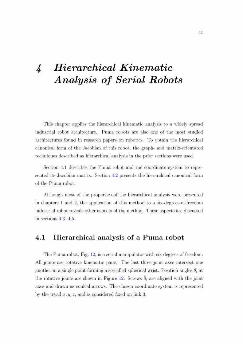
41
4 Hierarchical KinematicAnalysis of Serial Robots
This chapter applies the hierarchical kinematic analysis to a widely spread
industrial robot architecture. Puma robots are also one of the most studied
architectures found in research papers on robotics. To obtain the hierarchical
canonical form of the Jacobian of this robot, the graph- and matrix-orientated
techniques described as hierarchical analysis in the prior sections were used.
Section 4.1 describes the Puma robot and the coordinate system to repre-
sented its Jacobian matrix. Section 4.2 presents the hierarchical canonical form
of the Puma robot.
Although most of the properties of the hierarchical analysis were presented
in chapters 1 and 2, the application of this method to a six-degrees-of-freedom
industrial robot reveals other aspects of the method. These aspects are discussed
in sections 4.3- 4.5.
4.1 Hierarchical analysis of a Puma robot
The Puma robot, Fig. 12, is a serial manipulator with six degrees of freedom.
All joints are rotative kinematic pairs. The last three joint axes intersect one
another in a single point forming a so-called spherical wrist. Position angles θi at
the rotative joints are shown in Figure 12. Screws $i are aligned with the joint
axes and drawn as conical arrows. The chosen coordinate system is represented
by the tryad x, y, z, and is considered fixed on link 3.

4.1 Hierarchical analysis of a Puma robot 42
2θ
$1
2$
3$
3θ3θ2θ+
4$
6$θ5
θ6
θ4θ1
θ1
5$
x
f
h
z y
g
Figure 12: The Puma robot analyzed in this work. The screw $5, which is notexplicitly designated on the Figure is on the joint axis 5 in the middle of thespherical wrist.
6$
θ2
θ2+3
2+3θ2θ5$
1$
z
x
Figure 13: Side view (xz-plane) of the Puma.

4.1 Hierarchical analysis of a Puma robot 43
$1
θ4
θ4
$
$
3
5 $2
f
y
z
Figure 14: Frontal view (yz-plane ) of the Puma highlighting the spherical wrist.
The Jacobian of a Puma robot is a rather complex matrix-valued function,
especially when obtained from the Denavit-Hartenberg method. The complexity
of the Puma Jacobian imposes selecting some auxiliary variables to obtain their
elements recursively [Jr, Nugent e Saridis 1987]. However, using screw theory
with a good choice of the coordinate system a significantly sparser Jacobian can
be obtained [Hunt 1987]. This Jacobian, with the coordinate system sketched in
Figs. 12 and 15, is
J =
−s23 0 0 1 0 c5
0 1 1 0 −s4 c4s5
c23 0 0 0 c4 s4s5
−fc23 gs3 0 0 0 0
x14 0 0 0 0 0
−fs23 x′41 −h 0 0 0
(4.1)
where si = sin θi; sij = sin(θi + θj); ci = cos θi; cij = cos(θi + θj), etc. . . and
x14 = gc2 + hc23, x′41 = −(gc3 + h), letters f, h, g are the distances shown in

4.1 Hierarchical analysis of a Puma robot 44
4$6$
3$
2$
$1 $5
x
y
f
h
g z
Figure 15: A sketch of the Puma robot with all joint variables at initial posi-tion.The coordinate system highlighted has origin at the wrist centre and is fixedon link 3.
Fig. 12. The structure of the inverse Jacobian is [Hunt 1987]
J−1 =
0 0 0 0 × 0
0 0 0 × × 0
0 0 0 × × ×× × × × × ×0 0 0 × × ×0 × × × × 0
(4.2)
where × represents the non-null terms of the matrix. The values of the inverse
Jacobian is omitted here, as specific values of J−1 are not required by algorithm 1.
The matrix J−1 is presented in [Hunt 1987], including some pertinent comments.

4.2 Hierarchical canonical form 45
4.2 Hierarchical canonical form
We use the kinematic structure matrix Q, eq. (2.16), to rearrange the system.
The end-effector screw x = $n = [x1, x2, x3, x4, x5, x6]T is represented in the
coordinate system shown in Fig. 12, see details in [Hunt 1987].
Using Algorithm 1, the hierarchically rearranged linear system corresponding
to eq. (2.16) is
x1
q4
x2
x3
q5
q6
x6
q3
x4
q2
x5
q1
=
× × ×× × × × × ×
× × × ×× × ×
× × × × ×× × × × ×
× × ×× × ×
× ×× ×
××
x1
q4
x2
x3
q5
q6
x6
q3
x4
q2
x5
q1
(4.3)
Extracting only the terms relative to the forward kinematics, i.e. dropping rows
2, 5, 6, 8, 10 and 12, eq. (4.3) becomes
x1
x2
x3
x6
x4
x5
= J
q4
q5
q6
q3
q2
q1
where J =
1 c5 −s23
−s4 c4s5 1 1
c4 s4s5 c23
−h x′41 −fs23
gs3 −fc23
x14
(4.4)
Matrix J is the hierarchical canonical form of the Jacobian given by eq. (4.1).
In the following text, we describe how this hierarchical canonical form can be
4.3 Jacobian Inversion 46
explored to solve the rearranged system, eq. (4.4), i.e. to invert the Jacobian
by decomposition. In the sequence, we detail the inversion of J as well the
singularities of the robot architecture. Finally, section 4.5, we discuss other extras
advantages that may be obtained by using this hierarchical canonical form.
4.3 Jacobian Inversion
Equation (4.4) permits the inversion via smaller subsystems, which cannot
be performed directly on the original eq. (4.1). In other words, the hierarchical
canonical form lightens the computational efforts and errors of inverting a higher
dimensional matrix.
The process of inverting using subsystems takes the following steps: decompo-
sition of the system into subsystems, ordering of the subsystems, use of variables
obtained in prior steps and inversion of the diagonal block. Each subsystem is
associated with only one diagonal block and corresponds to the rows where this
diagonal block belongs to. The system, now decomposed, has to be solved se-
quentially. Bottom rows in eq. (4.4) have to be solved first, and upper rows have
to wait for the variables obtained in the earlier subsystems. The method, in fact,
is the same as the inversion of the Scara Jacobian using eqs. (1.5)-(1.7), but the
Puma robot Jacobian, due to its complexity, turn the advantages of the method
more explicit.
Once the system is subdivided and the subsystems are ordered, the process
continues with the flow of variables from prior subsystems to following subsys-
tems. An intermediate step waits for the availability of variables obtained in
previous steps, and, once solved, it turns more variables accessible to the next
steps. In this process, to solve a subsystem is basically to invert the diago-
nal block; when such inversion is not possible we can say that a singularity is
reached.
We illustrate the process of the flow of variables, described above, solving the

4.4 Hierarchical analysis 47
subsystem comprised by the rows 2 and 3 of eq. (4.4)[x2
x3
]=
[−s4 c4s5
c4 s4s5
] [q5
q6
]+
[1
0
]q3 +
[1
0
]q2 +
[0
c23
]q1 (4.5)
At this step, variables q1, q2, q3 must be a priori known, so the last three terms
can be transferred to the first member of eq. (4.5). Finally, the variables q5 and
q6 come from the inversion of the diagonal block[q5
q6
]=
[−s4 c4s5
c4 s4s5
]−1 {[x2
x3
]−
[1
0
]q3 −
[1
0
]q2 −
[0
c23
]q1
}(4.6)
The inversion via decomposition into subsystems implicitly underline a flow of
variables from past to future steps. In eq. (4.5) this flow is:
q1, q2, q3 →subsystem
rows 2 and 3→ q5, q6 (4.7)
In the hierarchical analysis approach, variables are not obtained all together in a
monolithic way, as e.g. inverting directly: q = J−1x; in contrast, they are revealed
gradually in small groups, one group at each step.
4.4 Hierarchical analysis
Hierarchical analysis is the kinematic analysis performed using the hierarchi-
cal canonical form of the Jacobian. First, we associate the hierarchical canonical
form with the condensation digraph of the rearranged kinematic matrix Q. Sec-
ond, using the graphical appeal of the condensation digraph derived from Q, we
describe the flow of variables discussed above. Finally, at the end of the section,
we discuss how each singularity affects the Puma robot.
The condensation digraph, Fig. 16, of the robot can be directly obtained from
eq. (4.3), instead of the procedures in section 2.2. The horizontal lines divide the
subsystems of the robot Jacobian. If we compare each subsystem described in
Fig. 16, we notice that the flow of variables in the subsystem corresponds to the
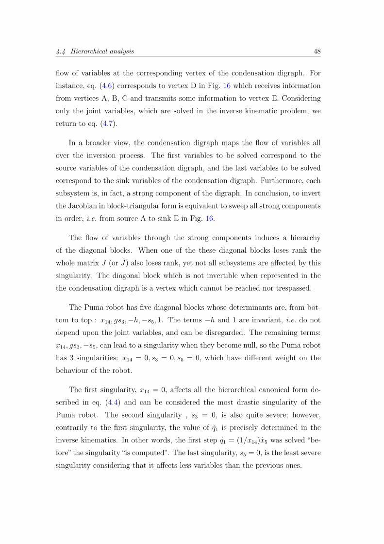
4.4 Hierarchical analysis 48
flow of variables at the corresponding vertex of the condensation digraph. For
instance, eq. (4.6) corresponds to vertex D in Fig. 16 which receives information
from vertices A, B, C and transmits some information to vertex E. Considering
only the joint variables, which are solved in the inverse kinematic problem, we
return to eq. (4.7).
In a broader view, the condensation digraph maps the flow of variables all
over the inversion process. The first variables to be solved correspond to the
source variables of the condensation digraph, and the last variables to be solved
correspond to the sink variables of the condensation digraph. Furthermore, each
subsystem is, in fact, a strong component of the digraph. In conclusion, to invert
the Jacobian in block-triangular form is equivalent to sweep all strong components
in order, i.e. from source A to sink E in Fig. 16.
The flow of variables through the strong components induces a hierarchy
of the diagonal blocks. When one of the these diagonal blocks loses rank the
whole matrix J (or J) also loses rank, yet not all subsystems are affected by this
singularity. The diagonal block which is not invertible when represented in the
the condensation digraph is a vertex which cannot be reached nor trespassed.
The Puma robot has five diagonal blocks whose determinants are, from bot-
tom to top : x14, gs3,−h,−s5, 1. The terms −h and 1 are invariant, i.e. do not
depend upon the joint variables, and can be disregarded. The remaining terms:
x14, gs3,−s5, can lead to a singularity when they become null, so the Puma robot
has 3 singularities: x14 = 0, s3 = 0, s5 = 0, which have different weight on the
behaviour of the robot.
The first singularity, x14 = 0, affects all the hierarchical canonical form de-
scribed in eq. (4.4) and can be considered the most drastic singularity of the
Puma robot. The second singularity , s3 = 0, is also quite severe; however,
contrarily to the first singularity, the value of q1 is precisely determined in the
inverse kinematics. In other words, the first step q1 = (1/x14)x5 was solved “be-
fore” the singularity“is computed”. The last singularity, s5 = 0, is the least severe
singularity considering that it affects less variables than the previous ones.

4.5 Other advantages 49
For illustration purposes, we will describe the last singularity in more detail.
When s5 = 0 the condensation digraph can be cut into two parts, Fig. 16, one
free from the singularity effects and the other affected by this singularity.
..
. .
.
.
.
. .
.
.
.xq
x q
x
q
q
x q
x
x
q51
4 2
6
3
5
2 6
3
1
4
Free part Affected part
vertex E
vertex Dvertex C
vertex B
vertex A (source)
(sink)
Figure 16: Condensation digraph of a Puma robot Jacobian based on the systemgiven by eq. (4.3). Vertex A of the condensation digraph is the source of thedigraph and vertex E is the sink of the digraph. A singularity at the vertex Ddivides the condensation digraph in two parts: one affected by the singularityand the other free from singularity effects
The affected part of Fig. 16 is composed by two types of variables: joint
velocities qi and end-effector directions xi. The joint velocities in the affected part
are those velocities which tends to have inadmissible higher magnitudes nearby
the singularity. On the other hand, end-effector directions in the affected part
are those directions which will certainly have errors, because the corresponding
joint velocities will not reach the high values required.
4.5 Other advantages
Above we described the two main advantages of the hierarchical analysis,
but other advantages are also a consequence of the hierarchical canonical form.

4.5 Other advantages 50
We will present here another two incidental advantages: direct inversion and
evaluation of the determinant.
Although the division of the whole system in smaller subsystems is a more
rewarding inversion procedure, we can also point out that the direct inversion of
J is better than the direct inversion of J . We can notice that the shape of the
system represented eq. (4.4) is improved when compared with eq. (4.1).
First, eq. (4.4) can be solved directly using methods such as LU decomposition
[Lucas, Tischler e Samuel 2000] with better results than eq. (4.1). The linear
system in eq. (4.4), in block-triangular form, has the pivoting process almost
done beforehand. Moreover, when the matrix has to be pivoted, the choice of
the pivot is limited to the elements of the diagonal blocks. Other point is that
“fill-in” generation (elements that were null and becomes non-null, i.e. becomes
filled in) is minimal when the matrix is its finest block-triangular form [Golub e
Loan 1983], which requires less storage capability.
Secondly, the determinant is easier to obtain in eq. (4.4) than in eq. (4.1).
Each diagonal block in eq. (4.4) for one term of the product which composes the
determinant. For instance,
det J = det J = (x14) · (gs3) · (−h) ·
det
[c4 −s4
s4 c4
] · (1) (4.8)

51
5 Hierarchical KinematicAnalysis of RedundantRobots
This chapter presents the hierarchical kinematic analysis in the context of
redundant manipulators. First, in section 5.1, the redundancy resolution is pre-
sented. Section 5.3 presents the extended Jacobian method, that is the most
affordable method to use the hierarchical kinematic analysis. In section 5.3.1,
this method is briefly compared with another important method in redundancy
resolution, the generalised inverse (or pseudoinverse) method.
To our purposes, the extended Jacobian method, as originally conceived, is
quite limited. Therefore, we propose a procedure for extending the Jacobian,
i.e. how to select the extra lines that shall be added to the matrix. Section 5.4
describes this method, designated here as globally constrained Jacobian method.
Despite this new method be based on the extension of the Jacobian, it has a
completely different approach to the redundancy resolution. In section 5.5, this
method is applied to the Roboturb manipulator.
5.1 Introduction to redundant robots
Robotic arms are defined as kinematically redundant when the number of
joints is greater than the number of degrees of freedom needed to describe a
specific task. The most general task of a manipulator is a general movement
of the end-effector along the three-dimensional Cartesian space. This general

5.1 Introduction to redundant robots 52
movement requires 6 degrees of freedom (d = 6) i.e. 6 independent variables to
be completely determined at every configuration. Therefore, every robot with
more than 6 independent joints is a redundant robot, as each joint is responsible
for an extra independent variable to the system. In a planar case (d = 3), on the
other hand, a manipulator with just four joints (f = 4) is always redundant no
matter which task is ascribed to it. The difference f − d is called the degree of
redundancy.
The interest in redundant manipulators has growing in the last two decades.
The main reason is that redundant manipulators can handle with movements in
confined or cluttered spaces. Other reason is the extra ability that redundant
manipulators have to avoid singularities, obstacles and joint limits. Another
reason is that many specific applications are derived from, or may be significantly
improved by, the use of redundant manipulators [Nenchev 1989]. We can cite
e.g. multi-fingered hands, cooperative robots1 [Hu e Goldenberg 1993], sheep
shearing [Trevelyan, Kovesi e Ong 1983] [Trevelyan 1992], and manipulation in
space [Hu e Vukovich 1998].
The first difficulty with redundant robots is in the design stage. Very few
industrial robots are redundant, so most of the redundant robots must be specif-
ically designed and manufactured by the interested part. At this stage, the de-
signer must choose the degree of redundancy of the robot. Higher degree of
redundancy has stronger disadvantages, such as higher weight, complexities in
the control system, and higher cost. However, Hollerbach (1985) shows that a
seven degrees of freedom manipulator can do the tasks described above. For
this reason, unless otherwise stated, we will consider only manipulators with one
degree of redundancy, f − d = 1 , in this work.
1Two or more robots together cooperating in performing a common task

5.2 Redundancy resolution 53
5.2 Redundancy resolution
After the path planning, the methods to deal with redundant and nonredun-
dant manipulators differ significantly. The path planning is, in few words, a quest
for a suitable path to perform the desired task. Once established in Cartesian
space, the path has to be converted to the joint space via inverse kinematics. This
step for a redundant manipulator is sometimes called the redundancy resolution
of the manipulator, i.e. the computation of the joint variables, as accurately as
possible, to follow the path previously defined. In general, the redundancy reso-
lution yields an infinite number of joint solutions corresponding to a desired end-
effector position/orientation. This multiplicity of solutions is the main difficulty
of redundant manipulators. The redundancy resolution may be also described as
the choice of one inverse kinematic solution among an infinitude of solutions.
Two approaches are suggested in the literature to the redundancy resolution:
the use of generalised inverses, such as the Moore-Penrose pseudoinverse [Klein
e Huang 1983], or the use of the extended Jacobian [Baillieul 1985] [Chang
1986] [Klein, Chu-Jenq e Ahmed 1995] i.e. a Jacobian with extra rows. The clas-
sical approaches cited above, namely the extended Jacobian and pseudoinverse
methods, come from a minimisation procedure. For instance, the Moore-Penrose
pseudoinverse method minimise the Euclidean norm of the vector composed by
the joint variables, which is closely related to the minimisation of the kinetic en-
ergy [Siciliano 1993]. The extended Jacobian method impose extra constraints,
but they are in general derived from a minimisation procedure.
The extended Jacobian method is based on adding more rows to the Ja-
cobian, and is described in more detail in section 5.3. Section 5.3.1 presents a
brief comparison between the extended Jacobian method and generalised inverses
methods. A more detailed comparison can be found elsewhere [Klein, Chu-Jenq
e Ahmed 1993], [Park, Chung e Youm 1994], [Baker e Wampler 1988]. A good
review on the use of pseudoinverses for redundancy resolution is found in [Klein,
Chu-Jenq e Ahmed 1995].
5.3 Extended Jacobian method 54
Section 5.4 describes the globally constrained Jacobian method, here pro-
posed, based on the interpretation of the geometry and kinematics of the manip-
ulator. The globally constrained Jacobian method is also based on an additional
row to the Jacobian matrix in order to invert it. In this sense, the globally
constrained Jacobian method has close similarity with the extended Jacobian
method; however, both methods have different formulations and philosophies as
will be described in the next sections.
5.3 Extended Jacobian method
The extended Jacobian method is based on imposing additional constraint
functions of the form h(q) = 0. The proponents of this method, Baillieul (1985)
and Chang (1986), use this extra constraint as a secondary task to be simultane-
ously satisfied. They also give formulations for converting minimisation criteria
into these constraint functions.
Once the functions h(q) = 0 are determined, one must solve simultaneously
the combined set of equations
x(t) = f(q(t)) (5.1)
0 = h(q)
where f(q(t)) represents the function which relates the joint positions q(t) and
the Cartesian positions of the end-effector x(t). Equations (5.1) can be solved
numerically at each point, as suggested by [Chang 1986] or, when h and f are
differentiable, an initial solution to eq. (5.1) can be propagated along a path by
solving the differential kinematic equation
Jeq =
[x
0
](5.2)
5.3 Extended Jacobian method 55
where Je was named by Baillieul (1985) as the extended Jacobian matrix defined
by
Je =
[J(q)
∂h(q)/∂q
](5.3)
The condition for the existence of a unique solution q in eq. (5.2) is that the
extended Jacobian matrix Je be nonsingular along the entire path. General spatial
manipulators with one degree of redundancy have J(q) as a 6 × 7 matrix, J6×7,
and Je is a 7 × 7 matrix. In this case h(q) is a scalar function of vector q.
Unless otherwise stated, this is the degree of redundancy that we consider in
this chapter; nevertheless, all methods described here are, mutatis mutandis,
applicable to higher degrees of redundancy.
Klein et al.(1993) asserts that the presence of algorithmic singularities is one
of the disadvantages of the method. Algorithmic singularities are those created
by the presence of the extra row and which were not present at the original
Jacobian J6×7. From eqs. (5.2) and (5.3) we noticed that det Je = 0 can have
solutions which are not related to the kinematics of the robot itself and are
purely related to the “intrusion” of the extra row ∂h(q)/∂q. In this sense, the
advantages of redundant robots cited above may be limited by some spurious
algorithmic singularities, possibly generated by a bad selection of the constraint
function h(q).
The choice of the “objective criterion h(q)” is described by Klein (1995) as a
rather complex task. The literature provides general objective criteria h(q) which
tend to be more appropriate to one or another problem, such as the avoidance of
obstacles, singularities or joint limits.
The most common objective criterion is [Klein, Chu-Jenq e Ahmed 1995]
h(q) =n∑
i=1
q2i (5.4)
Equation (5.4) is called the joint-range availability criterion because it tends to
keep the joints near their centre of travel and away from mechanical limits2. The
2We are considering that the joint angles origin are set at the centre of the travel of the

5.3 Extended Jacobian method 56
last row of eq. (5.3) will be then equal to 2 [q1 q2 · · · qn] = 2q
The equation which corresponds to the last row in eq. (5.2) is
∂h(q)/∂q = 0 (5.5)
Dividing eq. (5.5) by 2 and appending it to the original Jacobian generates the
extended Jacobian:
Je =
[J6×7(q)
q1 q2 · · · q7
](5.6)
The presence of all joint variables in the last row of Je is a clever way to avoid se-
lecting which variables are important to the performance of the robot and which
variables are not; however, the full last row increases the presence of unexpected
algorithmic singularities. Moreover, the full last row couples the associated di-
graph of eq. (5.6) perhaps more than necessary.
Despite these facts, the use of the extended Jacobian method has important
advantages over the pseudoinverse methods, and a comparison of both methods
will be presented next.
5.3.1 Comparison with generalised inverse methods
The generalised inverse methods are based on a minimisation of a criterion
to choose the best option, according to this criterion, among the infinitude of
possible solutions. Several generalised inverse methods exist [Doty, Melchiorri
e Bonivento 1993]; however, the most used generalised inverse is the Moore-
Penrose pseudoinverse or, for short, the pseudoinverse. This section will present
some comparative aspects of these methods in relation to the extended Jacobian
method.
The extended Jacobian method is claimed by some authors [Klein, Chu-Jenq
e Ahmed 1995] as being easier to set. The main goal of all these methods is to
joint. If this is not the case a simple adjustment can be done on eq. (5.4)
5.3 Extended Jacobian method 57
obtain a good performance between a sluggish manipulator and an unstable one.
In this aspect, the selection of an additional constraint can be easier than the
selection of suitable weight factors in the generalised inverse methods.
Other aspect is that the extended Jacobian method provides, under certain
conditions, a conservative movement, i.e. one closed path on the end-effector
space causes a closed path on the joint variables space. Baker & Wampler (1988)
demonstrate that the pseudoinverse methods cannot obtain conservative move-
ment while extended Jacobian methods guarantee conservative movement within
a simply connected region without internal singularities. This fact is reinforced
in simulations and experiments elsewhere [Nenchev 1989] [Klein e Huang 1983].
Similarly to the pseudoinverse solution, the extended Jacobian method, as it
was originally proposed, can be considered as a particular case of other formula-
tions. For example, Nenchev (1989) shows that the extended Jacobian method
is a particular case of the constrained least-square method. In reality, both ap-
proaches are closely intertwined. For instance, the problem of algorithmic singu-
larities, which is characteristic of extended Jacobian methods, is encountered also
in pseudoinverse-based solutions, such as the task-priority redundancy resolution
discussed in [Chiaverini 1997].
However, the difficulties of selecting precisely the function h(q), the coupling
of the associated digraph and the presence of unexpected algorithmic singularities
still remain. The selection of a suitable function h(q) at positional level is not
simple. General criteria, like the joint availability criterion of eq. (5.4), cannot
be widely applied. Most robot architectures demand for a specific function h(q).
These facts lead us to reconsider the extended Jacobian method. For these
reasons, we developed a method also based on the extension of the Jacobian
but with a different methodological perspective. To distinguish this method we
designate this variant as the globally constrained Jacobian method while keeping
the designation “extended Jacobian method” to the classical methods found in
the literature up to now. In fact, the globally constrained Jacobian method is an
“extended Jacobian method”. Their differences will be listed in the section 5.4.
5.4 Globally constrained Jacobian method 58
5.3.2 Hierarchical kinematic analysis using extended Ja-cobian method
As described above, the full last row of the classical extended Jacobian
method couples the associated digraph of eq. (5.6) perhaps more than necessary.
This strong coupling has two negative effects: singularities have a more complex
expression and are harder to predict and to avoid, and the use of hierarchical
kinematic analysis becomes less beneficial.
5.4 Globally constrained Jacobian method
The globally constrained Jacobian method, as the extended Jacobian method,
is a method based on appending an extra row to the Jacobian matrix; therefore,
avoiding generalised inverses and permitting hierarchical kinematic analysis. The
constraint, in this case, is not imposed considering a minimisation process or the
robot function h(q) at a positional level alone; instead, the extra row is selected
based on the task and on the geometry of the manipulator.
The crucial difference between both methods emulates the technical and philo-
sophical conflict between the choice of general methods in Kinematics, i.e. the
methods which can be applied to a wide class of mechanical architectures, and
particular methods, i.e. those fitted to (optimally) satisfy one specific architec-
ture and whose adaptation to another mechanism involves redesigns [Fanguella
e Galletti 1989]. In our case, the classical extended Jacobian method provides a
global kinematic solution to the problem while the globally constrained Jacobian
method provides a specific solution to each robot architecture.
The choice of this extra row in the globally constrained Jacobian method is
not based on an assumed position function, but rather on a velocity constraint.
We will illustrate the concept with an example: a redundant seven degrees-of-

5.4 Globally constrained Jacobian method 59
freedom robot. This kind of manipulators has a Jacobian matrix such as
J6×7 =[$1 $2 · · · $7
](5.7)
where each one of the seven columns is the 6 Plucker’s coordinates of the screw
$i corresponding to the joint variable qi [Hunt 1987]. The equation which corre-
sponds to the last row takes the general form
r = ~nq (5.8)
The variable r is a scalar, the redundancy parameter, which maps the “move-
ment” of the constraint plane whose normal is given by ~n. Vector ~n can be
e.g. ~n = e1 = [1 0 0 0 0 0 0] which reduces eq. (5.8) to a simpler form: r = q1.
In this case, the redundancy resolution is made by keeping control only of the
velocity of the first joint. For example, this velocity can be null; therefore, the
first joint is blocked and the remaining 6 joints are solved using the traditional
form of the inverse kinematics.
Comparing the extended row of the globally constrained Jacobian method,
eq. (5.8), and the extended row of the classical extended Jacobian method,
eq. (5.5), an important difference is perceived. Equation (5.5) imposes a con-
straint which is a hyperplane passing necessarily through the origin of the joint
space R7 spanned by the joint variables q1, q2, q3, q4, q5, q6, q7.
Figure 17 shows a projection of the joint space R7 into a 2-dimensional plane
corresponding to two generic variables qi and qj. Each inclined line corresponds
to the projected constraint. Distances ri are projections in this two-dimensional
subspace of some values of the redundancy parameter r.
The extended Jacobian method has no flexibility to vary r (and correspond-
ingly ri). In the extended Jacobian method the hyperplane representing the
constraint passes obligatorily through the origin of R7. In this case, the re-
dundancy parameter does not exist (r ≡ 0) and the following simple kinematic
interpretation is not feasible.

5.4 Globally constrained Jacobian method 60
r1
q j
q i
r4
r3
r2
r4
r3
r2
r1 < < <
extendedJacobianconstraint
Figure 17: Comparison of the constraints of the globally constraint Jacobianmethod and the classical extended Jacobian method seen from a 2-dimensionalprojection of the R7 space. Scalars ri are projections of the values of r in eq. (5.8).Negative values for r, and correspondingly ri are also possible.
5.4.1 The simplest choice ~n = ei
In fact, the simple choice ~n = ei can be suitable when the consequences of
this choice are known. In the remaining of this work we will adopt solutions of
the form ~n = ei explaining the reasons which lead us to the choice. However, this
is not the unique solution to the problem.
The above case leads to
~n = ei =⇒ r = qi (5.9)
which provides a strategy to avoid singularities. The Roboturb robot can serve as
an example. The Roboturb robot has three singularities, see details in section 5.5
and [Martins e Guenther 2001]. Two of these singularities are s4 = 0 and s6 = 0
which means that when q4, q6 = 0 (or π) the Jacobian matrix drops rank.
The proximity of a singularity can be monitored by the functions s4 and s6.
For example, when |s4| is near zero some joint velocities will become exceedingly

5.4 Globally constrained Jacobian method 61
large. Keeping |s4| > ε4 can avoid such situation, here ε4 is a scalar which
serves as a threshold chosen to obtain a certain degree of velocities around the
singularity. When this threshold is reached, the last row can be changed to a
more appropriate constraint like ~n = e4 = [0 0 0 1 0 0 0], =⇒ r = q4. As the
manipulator approaches an unsafe zone, the performance of the robot decreases.
A strategy to avoid this situation must be given. A way to control the redundancy
parameter is by imposing
r = −kq4
‖q4‖, k > 0 (5.10)
where q4 is the last velocity which the manipulator reached the subspace of the
Cartesian space which corresponds to the ball {q ∈ Rn|q4 ≤ ε4 in the joint space.
Details of this method of singularity avoidance can be found in [Martins, Simas
e Guenther 2001].
5.4.2 Algorithmic singularities
Algorithmic singularities are one of the problems which is derived from the
extended Jacobian method and some authors, e.g. [Klein, Chu-Jenq e Ahmed
1993], point out that this is the most critical problems with this method.
The globally constrained Jacobian method may also present algorithmic sin-
gularities but, as the added row is normally independent of the joint variables,
the mapping of these algorithmic singularities becomes quite easier.
Let us consider an added row in the form ~n = ei. In this case the algorithmic
singularities are avoided when the minor determinant excluding the added row
and the i-th column is kept non-null. This submatrix naturally will drop rank
only when the associated non-redundant robot, i.e. the robot with the i−joint
fixed, reaches a singular configuration. This type of singularity can be considered
troublesome, but it cannot be considered unexpected as it has a clear connection
with the robot geometry.
5.5 Hierarchy of the singularities of the Roboturb robot 62
5.4.3 Hierarchical kinematic analysis using globally con-strained Jacobian method
The globally constrained Jacobian method has the same features of the ex-
tended Jacobian method, as both methods rely on the the extension of the Jaco-
bian. However, as the design of this extra row has no direct relationship with a
positional constrained, the freedom of choice of this line is greater.
In the globally constrained Jacobian method, the extra row has normally two
basic characteristics: the row is quite simple such as ~n = ei, and normally is
independent of the positional parameters ~n 6= ~n(q).
Both characteristics lead to a minimal coupling of the associated graph of
Je and yield a better hierarchical kinematic analysis. The rearranged system has
smaller diagonal blocks, each one related to a unique singularity. The overlapping
of singularities in strongly avoided at this stage, whenever the robot architecture
permits, and unexpected singularities are minimised.
5.5 Hierarchy of the singularities of the Robo-
turb robot
The Roboturb robot is a serial manipulator with seven degrees of freedom
originally conceived to repair turbine blades [Guenther, Simas e Pieri 2000]. The
first joint is prismatic, and the remaining 6 joints are rotative. The last three
joint axes intersect one another in a single point forming a so-called spherical
wrist. Figure 18 illustrates the manipulator that will be analysed in this work.
Figure 19 shows a sketch of the manipulator architecture, and the chosen
coordinate system where screw theory methods are applied. This Figure remarks
the initial configuration of the robot i.e. qi = 0∀i.
Screws $i at joints are shown in Fig. 19. Position angles qi are associated
with each joint of the manipulator and have positive orientation shown in Fig. 19.

5.5 Hierarchy of the singularities of the Roboturb robot 63
Figure 18: The Roboturb manipulator
The first joint, represented by $1, is prismatic and has translational displacement
along the direction of $1. The chosen coordinate system is represented by the
triad x, y, z fixed on link 4. Figure 19 shows the coordinate system chosen and
the manipulator at the null position, i.e. at the position where all joint variables
are zero, qi = 0 for i = 1, 2, · · · , 7.
The Jacobian corresponding to Fig. 18 is
J =
0 −s34 0 0 1 0 c6
0 −c34 0 0 0 −s5 c5s6
0 0 1 1 0 c5 s5s6
−s34 d4c34 a2s4 0 0 0 0
−c34 d4c34 x24 a3 0 0 0
0 x14 0 0 0 0 0
(5.11)
where si = sin qi; sij = sin(qi + qj); ci = cos qi; cij = cos(qi + qj), etc . . . The

5.5 Hierarchy of the singularities of the Roboturb robot 64
a3
$7
$6
$3
$4
$5d
3
$2
$1
a2
a1
x
z
y
Figure 19: Coordinate system chosen to the Roboturb robot. The coordinatesystem is shown at the initial configuration i.e. the configuration where all thejoint variables qi are null. Notice that $1 corresponds to the prismatic jointdisplacement along the trail while the remaining six screws ($1−$7) are rotationaldisplacements.
symbols a1, a2, a3 are distances shown in Fig. 19.
Here x14 = a1 + a2c3 + a3c34 and x24 = a3 + a2c4 represent distances along
the x-axis from the spherical wrist centre to joints 1 and 2 axles, respectively.
This notation, based on [Hunt 1987], was also used for other Jacobians such as
the Puma robot.
The Jacobian of eq. (5.11) is extended by an extra row ~n = e1, as the main
positional movement of this manipulator is performed over the prismatic joint at
the first joint. This decision is in accordance with the kinematic conception of the
robot described in [Guenther, Simas e Pieri 2000]. This redundancy resolution
may be interpreted as: given the desired velocity of the manipulator over the
trail, q1(= r), the system is solved for the remaining velocities through inverse

5.5 Hierarchy of the singularities of the Roboturb robot 65
kinematics. This results in the extended Jacobian:
Je =
0 −s34 0 0 1 0 c6
0 −c34 0 0 0 −s5 c5s6
0 0 1 1 0 c5 s5s6
−s34 d4c34 a2s4 0 0 0 0
−c34 d4c34 x24 a3 0 0 0
0 x14 0 0 0 0 0
1 0 0 0 0 0 0
(5.12)
The structure of the inverse of the extended Jacobian is obtained numerically
using algorithm described in the appendix D
J−1e =
0 0 0 × 0 × ×0 0 0 0 0 × 0
0 0 0 0 0 0 ×0 0 0 × × × ×0 × × × × × ×0 × × × × × ×× × × × × × ×
(5.13)
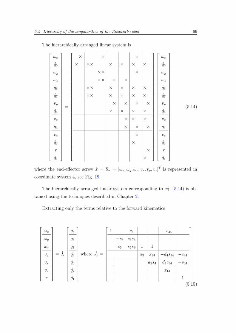
5.5 Hierarchy of the singularities of the Roboturb robot 66
The hierarchically arranged linear system is
ωx
q5
ωy
ωz
q6
q7
vy
q4
vx
q3
vz
q2
r
q1
=
× × ×× ×× × × × ×
×× ××× × ×
×× × × × ××× × × × ×
× × × ×× × × ×
× × ×× × ×
××
××
ωx
q5
ωy
ωz
q6
q7
vy
q4
vx
q3
vz
q2
r
q1
(5.14)
where the end-effector screw x = $n = [ωx, ωy, ωz, vx, vy, vz]T is represented in
coordinate system 4, see Fig. 19.
The hierarchically arranged linear system corresponding to eq. (5.14) is ob-
tained using the techniques described in Chapter 2.
Extracting only the terms relative to the forward kinematics
ωx
ωy
ωz
vy
vx
vz
r
= Je
q5
q6
q7
q4
q3
q2
q1
where Je =
1 c6 −s34
−s5 c5s6
c5 s5s6 1 1
a3 x24 −d4s34 −c34
a2s4 d4c34 −s34
x14
1
(5.15)

5.5 Hierarchy of the singularities of the Roboturb robot 67
Equation (5.15) has a strictly upper block-triangular form. The only 2 × 2
diagonal block has determinant −s6 which is associated to the so-called wrist
singularity of the manipulator. From bottom to top the hierarchy of special
configurations is (x14 = 0), (a2s4 = 0), (−s6 = 0). For instance x14 = 0 affects
all screw coordinates of the end-effector while s6 = 0 affects only ωx, ωy, ωz. The
linear velocity components vy, vx, vz of the end-effector are uniquely determined
even if s6 = 0. Physically, the spherical wrist singularity (s6 = 0) affects the
orientation of the end-effector but not its position nor linear velocity.
These facts become more evident when we extract only the terms relative to
the inverse kinematics
q5
q6
q7
q4
q3
q2
q1
=
XX��
J−1e
ωx
ωy
ωz
vy
vx
vz
r
(5.16)
where
XX��
J−1e =
1 × × × × × ×−s5 c5 × × × ×c5/s6 s5/s6 × × × ×
1/a3 × × ×1/(a2s4) × ×
1/x14
1
(5.17)
These results are quite similar to those obtained in [Martins e Guenther 2001]
where the Puma robot in the coordinate system of Hunt (1987) is analysed. In
fact, the Roboturb has an architecture similar to the Puma robot, but with the
shoulder eccentricity located at a different place. The Roboturb manipulator has
d3 located between joints 3 and 4, while the Puma manipulator has f (or d3

5.6 Final comments 68
according to the Denavit-Hartenberg convention) located between joints 1 and 4
axes.
5.6 Final comments
This chapter reinforced that the hierarchical kinematic analysis can be suc-
cessfully applied to redundant manipulators. The core of the problem is the use
of an extended Jacobian and then using Algorithm 1 to reorder the extended (and
square) Jacobian.
General positional criteria, such as the joint availability criterion of eq. (5.4),
couples the associated digraph of eq. (5.6) more than necessary and makes the
use hierarchical kinematic analysis less beneficial.
While the hierarchical kinematic method can be applied to any extended
Jacobian method, the results can be quite deceptive when the positional criteria
tend to couple all, or almost all, of the kinematic variables. The consequences
of this coupling are per se negative, e.g. increasing the presence of unexpected
singularities. For this reason, we provided a variant of the extended Jacobian
method which minimise this coupling and, as consequence, yields a more useful
hierarchical kinematic analysis.
At last, we observe that the obtained results, for the Roboturb manipulator,
are quite similar to those obtained in chapter 4 and in [Martins e Guenther 2001],
for the Puma robot, due to the similarity between both architectures.

69
6 Hierarchical KinematicAnalysis of Parallel Robots
This chapter deals with parallel robots and how the hierarchical kinematic
analysis may contribute to the kinematic solution of this kind of manipulators.
First, we describe the main differences between serial and parallel robots. In
the sequence, we present the steps needed to apply the hierarchical kinematic
analysis. Finally, the method is applied to a planar variant of the Stewart-Gough
platform.
Parallel robots have, in general, simpler inverse kinematics than direct kine-
matics. Other two differences between parallel robots and serial robots require
special attention before using the hierarchical kinematic analysis. First, singular-
ities of parallel robots are severer than the singularities of serial robots. Second,
the Jacobian matrix generally is not explicitly represented by the joint variables;
it is numerically obtained from internal and external (dot and cross) products of
vectors in the Cartesian space [Tsai 1999] [Valdiero et al. 2001].
Other characteristic of parallel robots is the presence of two types of singu-
larities: singularities which diminish the degrees of freedom of the manipulator,
and singularities which enlarge the degrees of freedom of the manipulator. Sin-
gularities in parallel robots are, in general, harder to predict and harder to avoid.
As the Jacobian matrix is numerically obtained, most of these singularities can
be even unexpected, so yielding hazardous consequences to on-line control.
6.1 Overview of the chapter 70
6.1 Overview of the chapter
In this chapter, we apply the hierarchical kinematic analysis to parallel robots.
Section 6.2 lists the prerequisites of the hierarchical kinematic analysis in order
to direct the focus of the next sections. These prerequisites were intrinsically
satisfied by the formulation applied to serial and redundant robots; however,
standard parallel robot kinematics algorithms do not satisfy these prerequisites.
Section 6.3 gives an overview of the structure of parallel robots and a brief history
of these manipulators, with special attention to Stewart-Gough platforms on sec-
tion 6.3.1. Section 6.5 describes the use of the Kirchhoff-Davies laws to obtain the
parallel robots kinematics. Section 6.6 shows how to improve the solution of the
linear system by using the hierarchical kinematic analysis. Section 6.8 shows the
close relationship between the hierarchical kinematic analysis of parallel robots
and their intrinsic decomposition into minimal Assur groups.
The first part of this chapter is based on the works of Davies (1981, 1983,
1995, 2000). The application of the Kirchhoff-Davies laws to the 3RRR planar
platform in this chapter, section 6.5, and in Appendix E follows closely [Campos
2001]. The Assur group theory, section 6.8, has several independent sources that
are specifically cited in section 6.8.
6.2 Requisites of the hierarchical kinematic anal-
ysis
Although not stated clearly in the earlier chapters, the hierarchical kinematic
analysis has two basic requisites:
• A linear system involving input and output velocities, e.g. in the form
x = Jq
• The elements of the matrix in this linear system must be explicitly known
for every configurations in space, i.e. J = J(q) or J = J(x).

6.3 Parallel robots: an introduction 71
The formalism used for serial robots in chapter 4 and the extension to redun-
dant robots in chapter 5 underline both of these requisites. Chapter 3 derives the
explicit relationship between each columns of the Jacobian matrix and the joint
variables, see for instance Fig. 11 at page. 36. For parallel robots, a method-
ology that encompasses both requisites is not widely used, as almost all of the
forms to obtain the Jacobian matrix are by internal and external (dot and cross)
products of vectors in the Cartesian space. An explicit (functional) dependence
relationship of the joint variables, or of the Cartesian coordinates, is not given.
The only method with attains both requisites seems to be the Kirchhoff-
Davies laws [Davies 1983] [Davies 1981] [Davies 1995] [Davies 2000] [Campos
2001].
The Kirchhoff-Davies laws, however, do not lead to a Jacobian matrix, at
least not directly. The method yields a linear system at a preliminary step in the
form [MN ][Ψ] = [0] that defines completely the (closed) kinematic chain but not
a particular mechanism. This mechanism is only defined when the actuators are
selected. The Kirchhoff-Davies laws is described in more detail in Appendix E.
A short description of these laws is in section 6.5.
6.3 Parallel robots: an introduction
Parallel manipulators differ from the more traditional serial robotic manipula-
tors by virtue of their kinematic structure. Parallel manipulators are composed by
one or more closed kinematic loops. Typically, these kinematic loops are formed
by two or more kinematic chains that connect a moving platform to a base, where
some of the joints of these kinematic chains does not have an actuator i.e. they
are passive. This kinematic structure allows parallel manipulators to be driven by
actuators positioned on, or near, the base of the manipulator [Tahmasebi 1992].
In contrast, serial manipulators, as those described earlier in this work, do not
have closed kinematic loops, and are usually actuated at each joint along the serial
linkage. In a serial chain, a significant part of the loads on the robot (including
6.3 Parallel robots: an introduction 72
link weights) is carried out by the actuators. The closer the base, the higher the
load the actuator has to overcome. In this sense, the first actuators have to be
more robust than the others. Reinforcing this fact, Trevelyan (1992) provides
a simple rule of thumb: each extra joint added to a serial robot approximately
doubles the weight of the manipulator.
Parallel manipulators distribute more evenly the loads among the actuators,
so they can weight less than serial manipulators. Hence, parallel manipulators
share the potential benefits associated with light weight construction, such as
high-speed operation and improved load to weight ratios. On the other hand,
parallel manipulators have smaller workspaces than serial manipulators of similar
size.
Tahmasebi (1992) describes the main advantages of parallel robots as
• Good rigidity
• Simple inverse kinematics
• High payload capacity
Nevertheless, they have the following extra disadvantages:
• Position and orientation of the moving platform are highly coupled.
• Their direct kinematics are difficult to solve.
• Most parallel robots require precise spherical joints, which are difficult to
manufacture at low cost.
Parallel robots architectures are usually of the platform-type, such as the
Stewart-Gough platform [Gough e Whitehall 1962] [Stewart 1966]. These parallel
robots are normally selected when serial robots are not suitable to the task. Two
reasons justify this choice: their generic applicability, and the avoidance of the

6.3 Parallel robots: an introduction 73
design process of a proper parallel robot to perform the task, as the design of
closed-chain mechanisms is not easy [Tischler, Samuel e Hunt 1995] [Tischler
1995] [Tischler, Samuel e Hunt 1998] [Tischler, Hunt e Samuel 1998]
Platform-type parallel robots are minimal kinematic chains, see details in
[Tischler, Samuel e Hunt 1995] [Tischler 1995], and for this reason are complex
when compared with non-minimal kinematic chains with the same number of
links. Non-minimal kinematic chains may be easier to build and be more ap-
propriate to a specific task. However, non-minimal kinematic chains require a
previous design. The designer needs firm grounds on kinematics and geometry as
well as some insight and patience to do this task.
6.3.1 Stewart-Gough platforms
Stewart (1966) proposes a mechanical architecture for a flight simulator,
whose variants are still used in Aeronautics. This mechanism was based on the
tyre testing machine devised by Gough & Whitehall (1962), apud [Tsai 2001].
Since then, the Stewart-Gough platform has also been applied in other areas, such
as milling machines, pointing devices, and underground excavation equipments.
Tsai (2001) provides more information at chapter 9 and references therein.
The Stewart-Gough platform has been extensively studied [Zhang e Song
1992] [Hunt e McAree 1998] [Ku 1999]. Generally, the Stewart platform has six
limbs, where each limb is connected to both the base and the moving platform
by spherical joints located at each end of the limb. The platform is typically
actuated by changing the lengths of the limbs.
Moreover, the closed-form direct kinematic solutions that have been reported
in the literature have generally required special forms of the Stewart-Gough plat-
form [Parenti-Castelli e Gregorio 1996] [Zhang e Song 1992]. In these special
forms, pairs of spherical joints may present design and manufacturing problems.
Some of these special forms require concentric spherical joints and a harder design
process, see comments on [Hunt e McAree 1998].

6.4 Kinematic problem of parallel robots 74
Due to the difficulties cited above, some of the current research focus on planar
parallel manipulators, specially on the planar variants of the Stewart platform,
e.g. [Wu e Huang 1996]. To illustrate the problem, we will exemplify the hier-
archical kinematic analysis of a planar mechanism: the 3RRR planar platform.
Nevertheless, the method described in the following sections may be generally
applied to any other planar, spherical or spatial mechanism.
6.4 Kinematic problem of parallel robots
A serial robot has, in general, no passive joints, i.e. all kinematic pairs are
actuated and we know in advance their positions, velocities and so on. Closed
kinematic chains, and in particular parallel robots, have passive joints constrain-
ing and cooperating to the desired end-effector behaviour. The parameters of all
of these passive joints are not known in advance; quite the opposite, the passive
joints parameters must be computed at each moment in function of the actuated
joints parameters.
This step, computation of the passive joints parameters in function of the ac-
tuated joints, is the crucial part of the parallel robot kinematics. This complexity
is derived from the closure of the chain that is not present in serial robots.
This chapter will be restricted to this problem and in how the hierarchical
kinematic analysis can improve the solution of this problem. Another goal is to
clarify the connection between the hierarchical canonical form and the kinematic
structure of the parallel robot.
In the next section, the Kirchhoff-Davies laws will be presented to prepare
the ground for the linear system at eq. (6.7) page 80. Kirchhoff-Davies laws lead
to a system satisfying the requirements described in section 6.2.
In the sequence, section 6.8, we correlate the hierarchical kinematic analysis
with the intrinsic kinematic structure of the parallel robot by using the classical
concept of the Assur groups [Assur 1952].
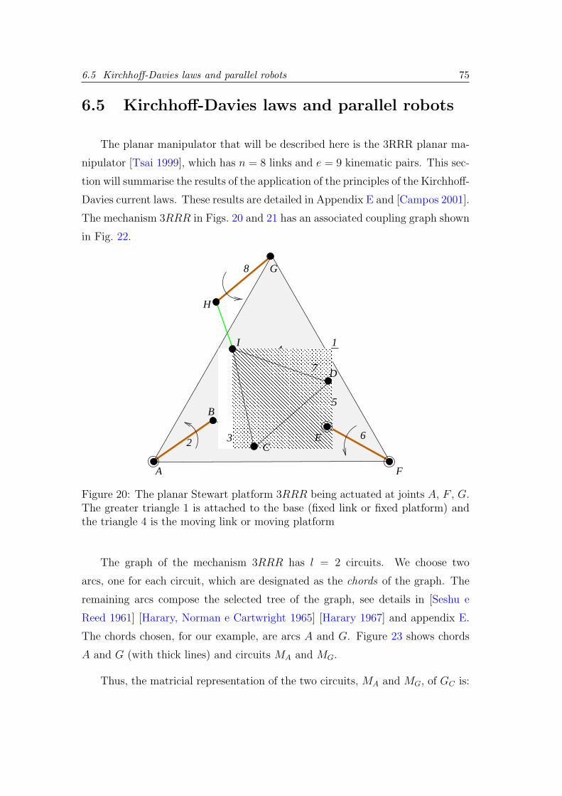
6.5 Kirchhoff-Davies laws and parallel robots 75
6.5 Kirchhoff-Davies laws and parallel robots
The planar manipulator that will be described here is the 3RRR planar ma-
nipulator [Tsai 1999], which has n = 8 links and e = 9 kinematic pairs. This sec-
tion will summarise the results of the application of the principles of the Kirchhoff-
Davies current laws. These results are detailed in Appendix E and [Campos 2001].
The mechanism 3RRR in Figs. 20 and 21 has an associated coupling graph shown
in Fig. 22.
41
� � � � � � � �� � � � � � � �� � � � � � � �� � � � � � � �� � � � � � � �� � � � � � � �� � � � � � � �
� � � � � � �� � � � � � �� � � � � � �� � � � � � �� � � � � � �� � � � � � �� � � � � � �
7
6
B
G
D
A F
5
2
I
H
3
8
CE
Figure 20: The planar Stewart platform 3RRR being actuated at joints A, F , G.The greater triangle 1 is attached to the base (fixed link or fixed platform) andthe triangle 4 is the moving link or moving platform
The graph of the mechanism 3RRR has l = 2 circuits. We choose two
arcs, one for each circuit, which are designated as the chords of the graph. The
remaining arcs compose the selected tree of the graph, see details in [Seshu e
Reed 1961] [Harary, Norman e Cartwright 1965] [Harary 1967] and appendix E.
The chords chosen, for our example, are arcs A and G. Figure 23 shows chords
A and G (with thick lines) and circuits MA and MG.
Thus, the matricial representation of the two circuits, MA and MG, of GC is:

6.5 Kirchhoff-Davies laws and parallel robots 76
2 θF
θH
θE
θB
θA
θG
8
7 1
4
3
5
6
B
CE
I
H
G
D
A Fk
h
�������
����� �������
x
y
Figure 21: Details of the the dimensions (lengths and angles) as well as of thechosen coordinate system to represent the mechanism 3RRR in the xy-plane
3
C
D
I4
5
6
1
A G
8
HB
7
E
F2
Figure 22: Coupling graph of mechanism 3RRR.

6.5 Kirchhoff-Davies laws and parallel robots 77
3
C
D
I4
5
6
1
A G
8
H
2
B
7
E
F
M MA G
Figure 23: Chords and circuits of the movement graph GM for the mechanism3RRR. This graph coincides with the coupling graph GC as there is no kinematicpairs with f > 1.
A B C D E F G H I
B =
[1
0
1
0
1
0
1
−1
1
−1
1
−1
0
1
0
1
0
1
]MA
MG
(6.1)
The movement graph GM for the mechanism 3RRR is also shown in Fig. 23;
indeed, there is no substitution of arcs, as each one of the e arcs has f = 1 degree
of freedom.
A B C D E F G H I
BM = B =
[1
0
1
0
1
0
1
−1
1
−1
1
−1
0
1
0
1
0
1
]MA
MG
(6.2)
As the mechanism 3RRR is planar, d = 3, we consider only three Plucker’s co-
ordinates: N ,P and Q [Hunt 1978]. Therefore, the matrix of normalised screws,
where the d rows represent the Plucker’s coordinates and the F columns represent
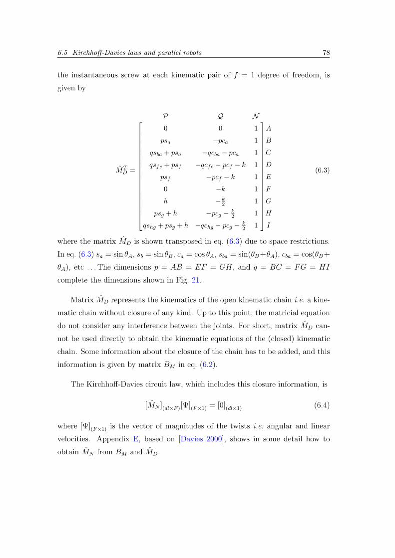
6.5 Kirchhoff-Davies laws and parallel robots 78
the instantaneous screw at each kinematic pair of f = 1 degree of freedom, is
given by
MTD =
P Q N
0
psa
qsba + psa
qsfe + psf
psf
0
h
psg + h
qshg + psg + h
0
−pca
−qcba − pca
−qcfe − pcf − k
−pcf − k
−k
−k2
−pcg − k2
−qchg − pcg − k2
1
1
1
1
1
1
1
1
1
A
B
C
D
E
F
G
H
I
(6.3)
where the matrix MD is shown transposed in eq. (6.3) due to space restrictions.
In eq. (6.3) sa = sin θA, sb = sin θB, ca = cos θA, sba = sin(θB +θA), cba = cos(θB +
θA), etc . . . The dimensions p = AB = EF = GH, and q = BC = FG = HI
complete the dimensions shown in Fig. 21.
Matrix MD represents the kinematics of the open kinematic chain i.e. a kine-
matic chain without closure of any kind. Up to this point, the matricial equation
do not consider any interference between the joints. For short, matrix MD can-
not be used directly to obtain the kinematic equations of the (closed) kinematic
chain. Some information about the closure of the chain has to be added, and this
information is given by matrix BM in eq. (6.2).
The Kirchhoff-Davies circuit law, which includes this closure information, is
[MN ](dl×F )[Ψ](F×1) = [0](dl×1) (6.4)
where [Ψ](F×1) is the vector of magnitudes of the twists i.e. angular and linear
velocities. Appendix E, based on [Davies 2000], shows in some detail how to
obtain MN from BM and MD.
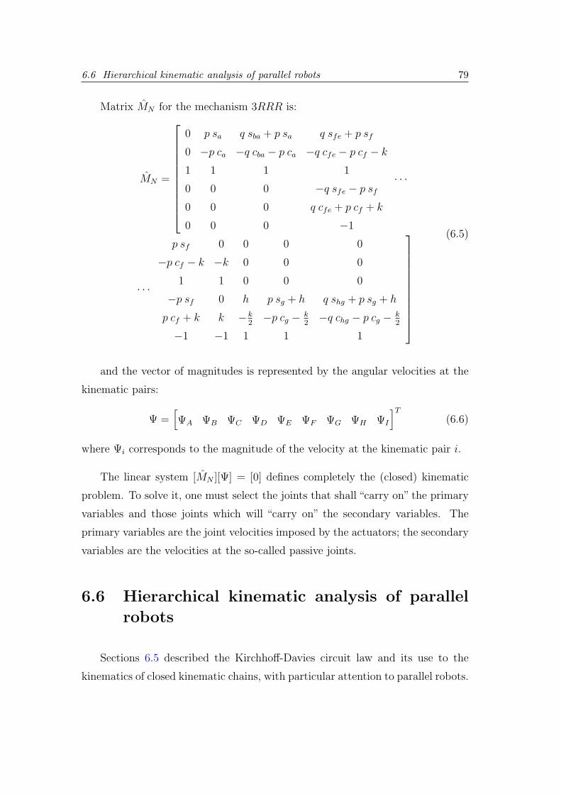
6.6 Hierarchical kinematic analysis of parallel robots 79
Matrix MN for the mechanism 3RRR is:
MN =
0 p sa q sba + p sa q sfe + p sf
0 −p ca −q cba − p ca −q cfe − p cf − k
1 1 1 1
0 0 0 −q sfe − p sf
0 0 0 q cfe + p cf + k
0 0 0 −1
· · ·
· · ·
p sf 0 0 0 0
−p cf − k −k 0 0 0
1 1 0 0 0
−p sf 0 h p sg + h q shg + p sg + h
p cf + k k −k2−p cg − k
2−q chg − p cg − k
2
−1 −1 1 1 1
(6.5)
and the vector of magnitudes is represented by the angular velocities at the
kinematic pairs:
Ψ =[ΨA ΨB ΨC ΨD ΨE ΨF ΨG ΨH ΨI
]T
(6.6)
where Ψi corresponds to the magnitude of the velocity at the kinematic pair i.
The linear system [MN ][Ψ] = [0] defines completely the (closed) kinematic
problem. To solve it, one must select the joints that shall “carry on” the primary
variables and those joints which will “carry on” the secondary variables. The
primary variables are the joint velocities imposed by the actuators; the secondary
variables are the velocities at the so-called passive joints.
6.6 Hierarchical kinematic analysis of parallel
robots
Sections 6.5 described the Kirchhoff-Davies circuit law and its use to the
kinematics of closed kinematic chains, with particular attention to parallel robots.

6.6 Hierarchical kinematic analysis of parallel robots 80
This section describes how to apply the hierarchical kinematic analysis to enhance
the solution of parallel robot kinematics.
The Kirchhoff-Davies circuit law leads to a relationship between each joint of
the kinematic chain, but it is not constrained to a specific choice of the actuators.
Each choice of the actuators underlines a different mechanism in a same kinematic
chain. Each mechanism has some particularity in the solution of the kinematic
equations, which leads to a different hierarchical kinematic analysis.
In section 6.8, we briefly indicate the relationship among the several hierar-
chical canonical forms generated by all the possible divisions of the variables, and
the Assur groups. A set of Assur groups is associated with each division. In this
section, we explore the differences in the hierarchical kinematic analysis among
the different mechanisms in a same kinematic chain. The kinematic chain, used
as example here, is again the 3RRR planar Stewart platform.
Equation (6.4), with eqs. (6.5) and (6.6), describes a homogeneous linear
system. The solution of this system, which is in fact the solution of the kinematics
of the parallel robot, requires the choice, among the Ψi in eq. (6.6), of d primary
variables i.e. those joints where the actuators are placed. The remaining (passive)
joints carry the secondary variables (joint velocities) which are the solution of the
system.
Equation (6.4) can be split in
[MN ]sec[Ψ]sec = −[MN ]pri[Ψ]pri (6.7)
where [MN ]sec is a (dl×dl) matrix and [MN ]pri is a (dl×d) matrix composed by the
columns of [MN ] corresponding to the primary joints. Vector Ψ is, accordingly,
subdivided into [Ψ]pri and [Ψ]sec.
In the 3RRR case, there is 6 rows and 9 columns in eq. (6.5) which can be
divided into a square 6× 6 matrix [MN ]sec and a 6× 3 matrix [MN ]pri. There is(93
)= 84 possible sets of primary joints, i.e. 84 different 6× 3 matrices [MN ]pri.
The subdivision of the matrix [MN ] into two parts has some similarity with
6.7 Permutation of the system 81
the serial manipulator system x = Jq. In this case, the analogue of the serial
manipulator Jacobian J is the square matrix [MN ]sec, the analogue of the vector
q of serial robots is the vector [Ψ]sec, and the analogue of the vector x of serial
robots is the vector formed by −[MN ]pri[Ψ]pri. This last vector may be considered
the sum of the effects of the all the actuators on the mechanism.
We will describe 3 choices of the actuators (i.e. 3 different mechanisms of the
same kinematic chain) and compare with their differences in the sequence.
6.7 Permutation of the system
The Algorithm 1 can rearrange the square matrix [MN ]sec to a block-triangular
form, unless it is undecomposable i.e. when the reachability matrix, eq. (2.6) at
page 19, is full.
However, prior to rearrange the square matrix the algorithm generates two
permutation matrices, Pr for rows and Pc for columns. While Pc permutation is
restricted to the first member of eq. (6.7), Pr permutation affects both sides of
eq. (6.7). The rearranged system is
Pr[MN ]secPcPcT [Ψ]sec = −Pr[MN ]pri[Ψ]pri (6.8)
which leads to
[MN ]sec[Ψ]sec = −Pr[MN ]pri[Ψ]pri (6.9)
So the right side of eq. (6.7) has to permute (Pr) its rows to maintain co-
herence with left side. As the dimensions of these matrices is not too large, in
general, these permutations can be done by inspection. In our example, the first
there rows of [MN ]pri are switch to the last three rows in sections 6.7.2 and 6.7.3.

6.7 Permutation of the system 82
6.7.1 Actuators at joints A, F , G
Figure 24 shows the mechanism 3RRR with actuators at joints A, F , G.
41
� � � � � � � �� � � � � � � �� � � � � � � �� � � � � � � �� � � � � � � �� � � � � � � �� � � � � � � �
� � � � � � �� � � � � � �� � � � � � �� � � � � � �� � � � � � �� � � � � � �� � � � � � �
7
6
B
G
D
A F
5
2
I
H
3
8
CE
Figure 24: Mechanism 3RRR actuated at joints A, F , G
The secondary variables correspond to the columns 2, 3, 4, 5, 8 and 9 of
eq. (6.5). The structure of the secondary matrix [MN ]sec is
[MN ]sec =
× × × × 0 0
× × × × 0 0
× × × × 0 0
0 0 × × × ×0 0 × × × ×0 0 × × × ×
(6.10)
Using algorithm 1 from chapter 2 at page 22, we notice that eq. (6.10) is un-
decomposable, as the reachability matrix, eq. (2.6) at page 19, is full. In other
words, no independent row and column permutation can lead matrix (6.10) to a
block-triangular form.

6.7 Permutation of the system 83
6.7.2 Actuators at joints D, E, F
Figure 25 shows the mechanism 3RRR with actuators at joints D, E, F .
41
� � � � � � � �� � � � � � � �� � � � � � � �� � � � � � � �� � � � � � � �� � � � � � � �� � � � � � � �� � � � � � � �
� � � � � � � �� � � � � � � �� � � � � � � �� � � � � � � �� � � � � � � �� � � � � � � �� � � � � � � �� � � � � � � �
6
B
C
G
D
A F
5
2
7
I
H
3
8
E
Figure 25: Mechanism 3RRR actuated at joints D, E, F
The secondary variables correspond to the columns 1, 2, 3, 7, 8, and 9 of
eq. (6.5). The structure of the secondary matrix [MN ]sec is
[MN ]sec =
0 × × 0 0 0
0 × × 0 0 0
× × × 0 0 0
0 0 0 × × ×0 0 0 × × ×0 0 0 × × ×
(6.11)
In this case the Algorithm 1 from chapter 2 has no effect, as the matrix is
already in its hierarchical canonical form. The matrix is a block-diagonal matrix
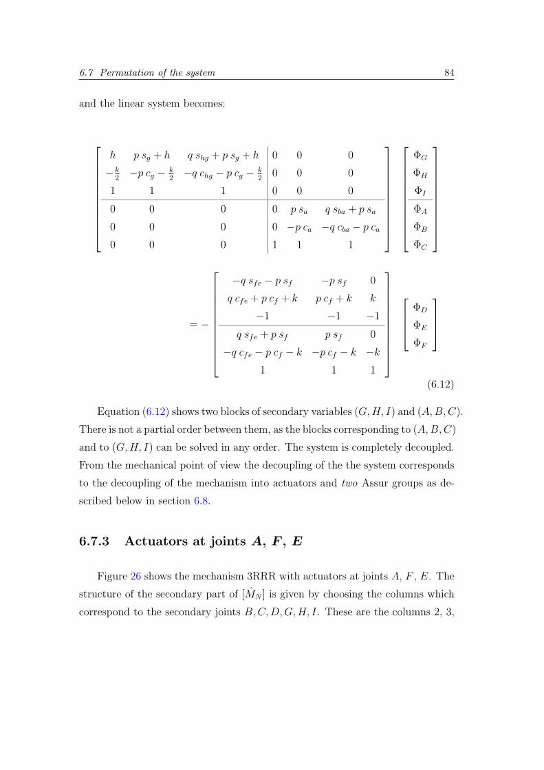
6.7 Permutation of the system 84
and the linear system becomes:
h p sg + h q shg + p sg + h 0 0 0
−k2−p cg − k
2−q chg − p cg − k
20 0 0
1 1 1 0 0 0
0 0 0 0 p sa q sba + p sa
0 0 0 0 −p ca −q cba − p ca
0 0 0 1 1 1
ΦG
ΦH
ΦI
ΦA
ΦB
ΦC
= −
−q sfe − p sf −p sf 0
q cfe + p cf + k p cf + k k
−1 −1 −1
q sfe + p sf p sf 0
−q cfe − p cf − k −p cf − k −k
1 1 1
ΦD
ΦE
ΦF
(6.12)
Equation (6.12) shows two blocks of secondary variables (G, H, I) and (A, B, C).
There is not a partial order between them, as the blocks corresponding to (A, B, C)
and to (G, H, I) can be solved in any order. The system is completely decoupled.
From the mechanical point of view the decoupling of the the system corresponds
to the decoupling of the mechanism into actuators and two Assur groups as de-
scribed below in section 6.8.
6.7.3 Actuators at joints A, F , E
Figure 26 shows the mechanism 3RRR with actuators at joints A, F , E. The
structure of the secondary part of [MN ] is given by choosing the columns which
correspond to the secondary joints B, C, D,G,H, I. These are the columns 2, 3,

6.7 Permutation of the system 85
41
� � � � � � �� � � � � � �� � � � � � �� � � � � � �� � � � � � �� � � � � � �� � � � � � �� � � � � � �
� � � � � � �� � � � � � �� � � � � � �� � � � � � �� � � � � � �� � � � � � �� � � � � � �� � � � � � �
6
B
C
G
D
A F
5
2
7
I
H
3
8
E
Figure 26: Mechanism 3RRR actuated at joints A, F , E
4, 7, 8, 9 in eq. (6.3). The structure of this square matrix is
[MN ]sec =
× × × 0 0 0
× × × 0 0 0
× × × 0 0 0
0 0 × × × ×0 0 × × × ×0 0 × × × ×
(6.13)
Using Algorithm 1 from chapter 2 at page 22, system (6.4) rearranged be-
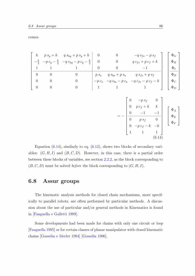
6.8 Assur groups 86
comes
h p sg + h q shg + p sg + h 0 0 −q sfe − p sf
−k2−p cg − k
2−q chg − p cg − k
20 0 q cfe + p cf + k
1 1 1 0 0 −1
0 0 0 p sa q sba + p sa q sfe + p sf
0 0 0 −p ca −q cba − p ca −q cfe − p cf − k
0 0 0 1 1 1
ΦG
ΦH
ΦI
ΦB
ΦC
ΦD
= −
0 −p sf 0
0 p cf + k k
0 −1 −1
0 p sf 0
0 −p cf − k −k
1 1 1
ΦA
ΦE
ΦF
(6.14)
Equation (6.14), similarly to eq. (6.12), shows two blocks of secondary vari-
ables: (G, H, I) and (B, C, D). However, in this case, there is a partial order
between these blocks of variables, see section 2.2.2, as the block corresponding to
(B, C, D) must be solved before the block corresponding to (G, H, I).
6.8 Assur groups
The kinematic analysis methods for closed chain mechanisms, more specif-
ically to parallel robots, are often performed by particular methods. A discus-
sion about the use of particular and/or general methods in Kinematics is found
in [Fanguella e Galletti 1989].
Some developments had been made for chains with only one circuit or loop
[Fanguella 1995] or for certain classes of planar manipulator with closed kinematic
chains [Gosselin e Merlet 1994] [Gosselin 1996].

6.8 Assur groups 87
The different behaviour presented by the kinematic chain when different actu-
ators are selected underline the intrinsic character of each mechanism derived. In
fact, this diversity can be explained using Assur groups [Assur 1952] [Manolescu
e Manafu 1963] [Baranov 1985] [Artobolevski 1988]
The technique of Assur groups [Manolescu 1968] [Hunt 1983] [Fanghella e Gal-
letti 1990] [Innocenti 1995] tries to decouple the kinematic equations from com-
plex kinematic chains into smaller modules whose behaviour can be more easily
studied. This technique is quite widespread for planar kinematic chains, mainly
the graphical approach [Baranov 1985]. However, computational approaches can
be already found in [Zablonski, Belokonev e Tchekin 1989] [Martins e Macie
1996] [Martins e Macie 1996].
Manolescu (1963,1968) defines an Assur group as an open subset which can
be added to a kinematic chain without affecting the mobility of the chain. The
simplest planar Assur group is the binary dyad, see a pair of them in Fig. 27. More
complicated Assur groups, both planar and spatial, can be found for instance
in [Tischler 1995]. If the unconnected joints of an Assur group were attached
directly to a base, a kinematic chain with zero degree of freedom would result.
Assur groups can be divided into minimal and non-minimal Assur groups.
The latter ones may be divided into smaller (fewer number of bodies) Assur
groups. The first ones are those which cannot be divided into minimal Assur
groups. For example, Fig. 28 shows a non-minimal Assur group and highlights
its decomposition into two minimal Assur groups, in this case two dyads.
Other division of planar Assur groups is relative to the order of these groups
[Martins e Macie 1996] [Martins e Macie 1996]. For the planar Assur groups
described in this work, Figures. 27 and 28 show first order Assur groups, while
Fig. 29 show a second order Assur group. The solution of higher order Assur
groups is, both graphically and computationally, more complex than lower order
Assur groups [Martins e Macie 1995]. The concept of order is generalised to any
spatial Assur group in [Tischler 1995]
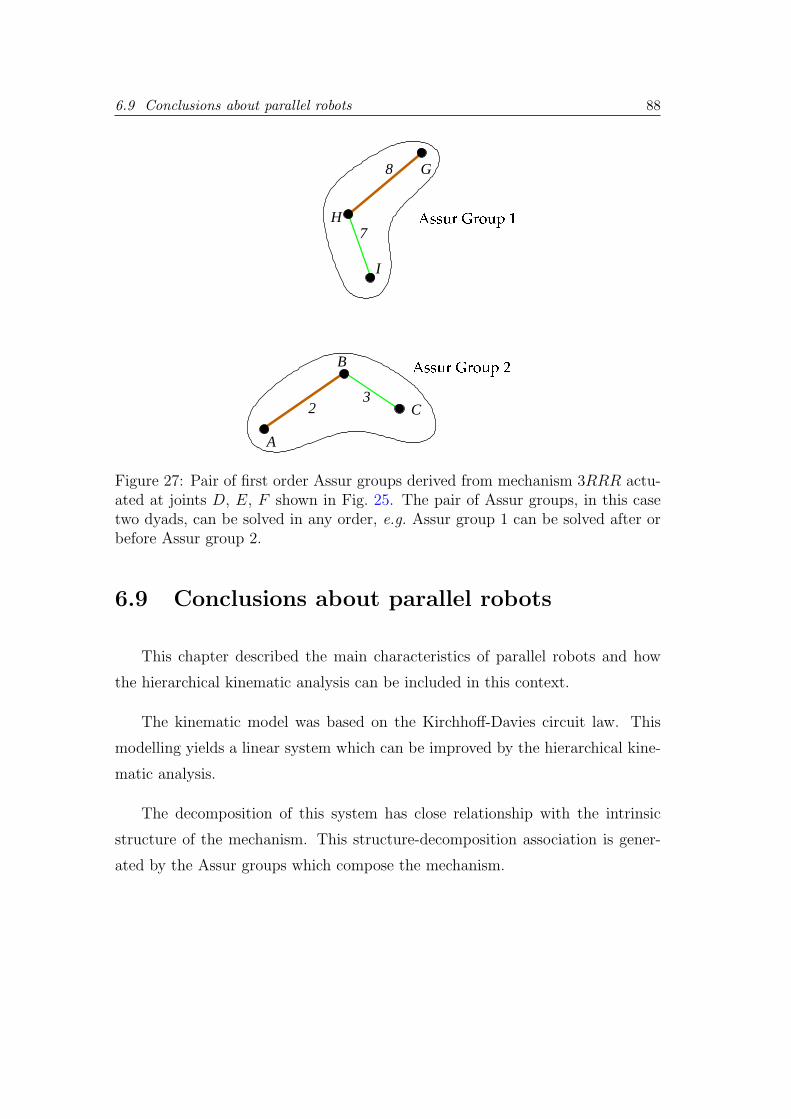
6.9 Conclusions about parallel robots 88
B
C
G
A
7
I
H
3
8
2
���������������� ��
���������������� ��
Figure 27: Pair of first order Assur groups derived from mechanism 3RRR actu-ated at joints D, E, F shown in Fig. 25. The pair of Assur groups, in this casetwo dyads, can be solved in any order, e.g. Assur group 1 can be solved after orbefore Assur group 2.
6.9 Conclusions about parallel robots
This chapter described the main characteristics of parallel robots and how
the hierarchical kinematic analysis can be included in this context.
The kinematic model was based on the Kirchhoff-Davies circuit law. This
modelling yields a linear system which can be improved by the hierarchical kine-
matic analysis.
The decomposition of this system has close relationship with the intrinsic
structure of the mechanism. This structure-decomposition association is gener-
ated by the Assur groups which compose the mechanism.
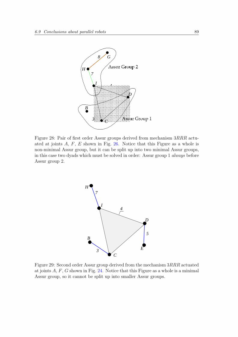
6.9 Conclusions about parallel robots 89
4
� � � � � � �� � � � � � �� � � � � � �� � � � � � �� � � � � � �� � � � � � �
� � � � � �� � � � � �� � � � � �� � � � � �� � � � � �� � � � � �
B
G
D
7
I
8 ������������ �����
������������ �����
3
H
C
Figure 28: Pair of first order Assur groups derived from mechanism 3RRR actu-ated at joints A, F , E shown in Fig. 26. Notice that this Figure as a whole isnon-minimal Assur group, but it can be split up into two minimal Assur groups,in this case two dyads which must be solved in order: Assur group 1 always beforeAssur group 2.
4
B
C
E
D
5
7
I
H
3
Figure 29: Second order Assur group derived from the mechanism 3RRR actuatedat joints A, F , G shown in Fig. 24. Notice that this Figure as a whole is a minimalAssur group, so it cannot be split up into smaller Assur groups.
90
7 Conclusions
This thesis develops the hierarchical kinematic analysis for serial, redundant
and parallel robots. The hierarchical kinematic analysis is a method based on
digraphs which leads the Jacobian matrix to a better form, the hierarchical canon-
ical form, to the analysis and resolution of the (inverse) kinematics of a wide class
of manipulators.
Some of the characteristics of the hierarchical kinematic analysis are:
• the determinant is easier to obtain in the hierarchical canonical form.
• the hierarchy of diagonal blocks induces a hierarchy of singularities.
• the concept of flow of variables is developed.
• the variables are classified as free or affected variables according to each
singularity. This classification has a direct correlation with the flow of
variables.
• the pivoting process in a numerical LU decomposition [Golub e Loan 1983]
of an upper block-triangular matrix is almost done without aggregating
errors to the solution.
• the inversion of a 6×6 Jacobian matrix is, in general, substituted by simpler
scalars or 2× 2 diagonal submatrices inversions.
• In the neighbourhood of a singularity, not all Cartesian velocities need
to be changed or adapted. Some may follow the path planning without

7.1 Perspectives and further work 91
modifications, even when the online control system alerts the proximity of
a singularity.
In chapters 5 and 6, the hierarchical kinematic analysis is extended to re-
dundant and parallel robots. Both of these extensions required a review of the
current methods of kinematic solution. For the redundant robots, we derived a
variant of the extended Jacobian method to the redundancy resolution. For par-
allel robots, we had to adapt the Kirchhoff-Davies laws to solve for the passive
joints parameters.
The method was applied to classical manipulators, such as the Puma robot
and the 3RRR planar variant of the Stewart-Gough platform. In both cases we
derive orignal correlations of the intrinsic geometrical structure of these manipu-
lators. For the redundant robot analysis, we applied to a new robot architecture,
the Roboturb manipulator for repairing eroded turbine blades [Guenther, Simas e
Pieri 2000] [Martins e Guenther 2001], designed as a redundant robot for confined
workspaces at the UFSC.
7.1 Perspectives and further work
Other topics are related to this thesis are worthy to mention. We present
here a list of possible new topics and enhancements of the work of the thesis.
• Development of a methodology and/or some criteria to derive a screw coor-
dinate system which can decouple the maximum number of input variables
for any manipulator. For instance, given a Denavit-Hartenberg Jacobian,
the application of the hierarchical kinematic analysis directly on this Jaco-
bian may suggest an appropriate coordinate system to refine the analysis.
In parallel some criteria to select the “best” coordinate system may be pro-
vided.
7.1 Perspectives and further work 92
• Analysis of the intrinsic singularities of redundant robots serial chain to
provide a strategy to singularity avoidance using the globally constrained
Jacobian method.
• Formalisation of a singularity avoidance technique, expanding the method
used in [Martins, Simas e Guenther 2001], to singularities which depend
upon a conjugation of two or more joint variables as x14 = gc2 + hc23 = 0
of the Puma robot, chapter 4.
• Expansion of the globally constrained Jacobian method to provide strategies
for general manipulators in constrained or confined workspaces.
• Integration between the hierarchical kinematic analysis and the path plan-
ning.
• Integration between the hierarchical kinematic analysis and the design of
control algorithms specific for a robot architecture.
• Application of similar results to the statics of mechanisms, including serial
and parallel robots, following the duality between statics and kinematics
and the Kirchhoff-Davies current laws [Davies 1983].
• Extension of the Algorithm 1 to the dynamic equations, as those listed
in [Tischler et al. 2000].
• Extension of the above procedures to a specific manipulator comparing
performance of the several choices of coordinate systems.
• Comparison among different manipulator configurations Jacobian matrices
in the rearranged form.
• Generalisation of the combinatorial results obtained through a digraph ap-
proach to a more generic scope. For instance using bipartite graphs and
matroids [Murota 2000] [Murota 1987]. A good possibility is the use of the
combinatorial canonical form cited in [Murota e Scharbrodt 1998].
7.1 Perspectives and further work 93
• Experimentation with more parallel robot architectures, specially spatial
manipulators.

94
APPENDIX A -- Screw Theory Basics
A.1 Kinematics and Statics of a rigid body
A review of some properties of the rigid body motion and static equilibrium
must precede the description of screw theory. The properties presented in this
section are the basis of the theory described in section A.2.
A body is considered rigid if it satisfies the rigidity condition i.e given any
pair of distinct points P (xP , yP , zP ) and Q(xQ, yQ, zQ) in the body the distance
d(P, Q) =√
(xQ − xP )2 + (yQ − yP )2 + (zQ − zP )2
is constant and independent of the time.
Kinematics and Statics of a rigid body have some similarities. Nonetheless
it is rare to observe in undergraduate textbooks a closer relationship between
Statics and Kinematics. However these similarities (more precisely dualities) are
crucial for a deep understanding of both areas.
Some connections between Statics and Kinematics (of rigid bodies) appear
at first glance. For instance the presence of a free vector and a line vector in
both areas. Forces and angular velocities are examples of line-vectors. They
have a line of action where they can slide freely without changing the static
and/or kinematic state of the body. On the other hand, couples and translational
velocities are examples of free vectors. Free vectors are those that do not depend
upon a specific point of application. Section A.1.2 for Statics and section A.1.3

A.1 Kinematics and Statics of a rigid body 95
for Kinematics describe the application of these concepts. Section A.1.1 will give
more detail about line vectors and free vectors.
Section A.1 introduces some concepts from Vectorial Mechanics. Most of
the following texts include ipsis litteris extracts from Coe (1938), for instance
Theorems 1 and 2.
A.1.1 Line vectors and free vectors
From High School Physics two vectors are considered equal if and only if they
have same direction, same sense along this direction and same length. It is often
adequate to combine other ideas in a same concept or be more specific when
dealing with a physical concept.
In Mechanics it is convenient to restrict the definition above to a “free vector”
as there are no constraints imposed on the “application point” of the physical
quantity carried out by this vector. In other words a free vector depends only
upon a direction, a sense and a length. Examples of free vectors are the translation
of a rigid body, the force of gravity in a small region on the earth’s surface and
the velocity of light from a distant star (e.g. sunbeams).
A line vector, also called “sliding vector”, is a combination of a straight line,
a sense along this line and a length. Two line vectors will be equal only if they lie
along the same axis, point in the same direction and have same length. Examples
of line vectors are the angular velocity of a body at any instant as well as forces
acting on a rigid body.
Another class of vectors is called attached vectors. An attached vector is a
vector associated with a specific point of application. Examples include velocity
profiles on a fluid flow, forces applied to a deformable body and the force of
gravity throughout the solar system. Rigid body Statics and Kinematics has no
examples of attached vectors so no further mention of attached vectors will be
given in this work.

A.1 Kinematics and Statics of a rigid body 96
The operation of addition, subtraction, internal and external (dot and cross)
multiplication of two vectors are performed on line and attached vectors exactly
as if they were free vectors. The result of these operations, when a vector, is
thought of as a free vector unless otherwise specified.
A.1.2 Statics
Any force vector field (including possibly some couples) can be substituted by
a resultant force F and a resultant moment (or couple) MP relative to a certain
point. Due to the sliding characteristic of the force vectors the same resultants
will be obtained if F is applied to any point along its line of action (Fig. 30). The
classical result in Statics is
F
F
F
F
ω
ω
ω
ω
(b)(a)
Figure 30: Line-vectors a) Forces b) Angular velocities.
Theorem 1 ( [Poinsot 1806]) Given a set of forces and pure couples applied
to a rigid body it is always possible to find a line along which the resultant force
and the resultant moment vectors will be directed.
The line mentioned in Theorem 1 is called Poinsot’s line. It is unique unless
F ≡ 0 (pure couple)1. The Poinsot’s line does not necessarily intersects any
1Using projective geometry it can be said that the pure couple is a force whose line of actionis at infinite
A.1 Kinematics and Statics of a rigid body 97
material point of the body. It only depends upon the external forces and couples
applied to the body. The shape of the body and even its convexity or continuity
are immaterial for the computation of the Poinsot’s line.
Couples can always be given as force binaries. The characteristics of a couple
are the magnitude of the pair the forces, the orientation of the plane where the
opposite forces actuate and their distance. The couple can be applied at any
material point on the body without affecting the static equilibrium of the body.
These facts characterize the couple as a free vector2.
A.1.3 Kinematics
Any rigid body movement can be decoupled in translational and rotational
parts. The velocity vector field in a rigid body can be substituted by a“resultant”
translational velocity3 τ and a “resultant” angular velocity ω relative to a certain
coordinate system. Due to the line-characteristic of the angular velocity vectors
this result will not be affected if ω is displaced along its line of action. The
classical result in instantaneous Kinematics is
Theorem 2 ( [Mozzi 1763]) The velocities of the points of a rigid body at any
instant are what they would be if the body were rotating about a certain fixed axis
and simultaneously had a motion of translation along this axis.
Chasles in 1830 expanded Theorem 2 to any finite displacement of a rigid
body. Today Theorem 2 is often refereed as Chasles-Mozzi’s Theorem or simply
Chasles’ Theorem. This line is unique unless ω ≡ 0 (pure translation). Similarly
to section A.1.2 this line do not necessarily intersects any material point of the
body.
2A free vector is defined as a infinite pitch screw, section A.23We use τ instead of the normally accepted v for two reasons:
• to reinforce the translational aspect of this velocity and
• to avoid confusion later when we represent a screw as a dual vector $ = (u, v)
A.2 Screw Theory 98
Translational velocity vectors are normally, in literature, associated to the
centre of mass of the body. This division decouples translational and rotational
kinetic energies and, in this sense, has some didactic appeal. The translational
velocity represents the translational “state”of the whole body and not of a specific
point. Any point pertaining to this body has the same translational velocity. The
resultant velocity field differs from point to point in virtue of the rotational com-
ponent of the velocity. The rotational component of the velocity is proportional
to the perpendicular distance from the point to the Chasles’ line. The transla-
tional velocity vector τ is another example of free vector as it is independent of
the point of application.
A.2 Screw Theory
There is a correlation or similitude of procedures relating Theorems 1 and 2.
This correlation was first discovered and formalised by Ball (1900) and remained
untouched for decades until Dimentberg (1948) and Hunt (1978) recover this topic
applying it to the theory of mechanisms.
The angular velocity ω and the linear velocity vector vP of a point P on
a moving body are three dimensional vectors. They can be assembled into a
six-dimensional vector $t called twist. The resultant force F and the couple C
acting at a point on the body can be assembled into a similar six-dimensional
vector $w called wrench. The mathematics of these vector pairs as well as their
physical and geometrical interpretation, also called dual vectors, is known as screw
theory, see Ball (1900), Hunt (1990) and Phillips (1984,1990). A mathematical
formalism known as a dual vector algebra is described in Dimentberg (1948), Woo
& Freudenstein (1970) and Bottema & Roth (1979). An algebraic treatment of
screw theory can also be found in Murray et al.(1994) or Selig (1996).
A.2 Screw Theory 99
A.2.1 Twists × Wrenches
A.2.1.1 Twists
Kinematics is based on the concept of velocity. Velocity of a rigid body,
however, has double meaning as the rigid body generally translates and rotates
simultaneously.
Thus angular velocity ω and translational velocity τ of the body must be
differentiated. Lemma 10, section B, shows how to uniquely represent τ and ω
via a dual vector $t = (ω;vP ), composed by the angular velocity ω of the whole
body and the linear velocity vP of a point P attached to the body. Both velocities,
ω and vP , need to be represented in the same coordinate system. On the Chasles’
line, and only there, ω and vP will be parallel. Moreover vP will have the same
value τ on any point along the Chasles’ line.
Definition 3 A twist is a dual vector $t = (ω;vP ) composed by the angular
velocity ω of the body and the linear velocity vP of a point P attached to the body,
both vectors represented in the same coordinate system.
The six-vector $t = (ω;vP ) = (ω;vQ + rQP ×ω) relative to a generic point P
is called the twist of the motion. The displacement vector rQP = P − Q relates
the point where the linear velocity vQ is a priori known (Q) and the desired point
(P )4. The twist is normally represented in ray order, see section A.2.5.
The second part (after “;”) represent the velocity of a point in the body in-
stantaneously coincident with the origin of the frame [Hunt 1978]. This particular
choice has some advantages, specially in the definition of the screw coordinate
transformation (section A.3). The symbol ; just separates two vectors that have
different physical dimensions. For instance ω can have dimension rad/s and vP
dimension m/s.
4Neither P nor Q have to be on the Chasles’ line.

A.2 Screw Theory 100
A.2.1.2 Wrenches
Statics of a rigid body is associated with (external) loads applied to this body.
The term load, as the term velocity discussed in section A.2.1.1, has also a double
meaning. A load can be a force or a couple (binary, moment of a force).
It is a common practice in elementary Statics to select an adequate point and
perform, relatively to this point, the summation of forces and summation of mo-
ments. However, differently from the twist case, the wrench free vector (resultant
couple C) varies from point to point and the wrench line vector (resultant force
F ) is independent of the chosen point. On the Poinsot’s line (and only there, see
section B) C and F are parallel.
Definition 4 A wrench is a dual vector, $w = (F ; MP ), composed by the resul-
tant (external) force F applied to a body and the resultant couple MP computed
at a point P of the coordinate system where both vectors are represented.
The vector pair $w = (F ; MP ) = (F ; MQ + rQP × F ) is the dual vector
associated with the static state of the system at P starting from an a priori
known summation of couples at a different point Q. This order of the vectors is
called ray order, see section A.2.5.
A wrench is represented in relation to the origin of the coordinate system
unless otherwise stated. This is also not obligatory but it is convenient [Hunt
1978].
A.2.2 Screws
A twist and a wrench are represented by a purely geometrical object called
screw plus a (dimensional) magnitude.
Definition 5 A screw $ is a geometrical entity composed by a line and a number
h called pitch which has length dimension.

A.2 Screw Theory 101
The relationship between a screw and a twist or between a screw and a wrench
is grosso modo similar to the notion of a vector as an entity having magnitude and
direction and its representation of the velocity or force acting on a body in space.
Any physical quantity that requires an line of action and a pitch can represented
by a screw. The same screw can be used indistinctly to represent a twist or a
wrench applied to a body. The dimension of the magnitude (for instance rad/s
and N) makes the distinction.
The notion of pitch h is associated with the relationship between both quan-
tities along the screw axis. In kinematics h = τ/ω. In statics h = C/F . In both
cases these quotients only make sense when both vectors are parallel i.e. along
the Chasles’ line (where vP = τ) or Poinsot’s line (where MP = C), respectively.
See Fig. 31.
C
F
Chasles’ line Poinsot’s line
ω
τ
Figure 31: Chasles’ line and Poinsot’s line.
We now state an important Lemma
Lemma 6 Any screw can be represented by a dual vector $ = (u; v) where the
A.2 Screw Theory 102
pitch can be calculated by
h =u · vu · u
(A.1)
and the minimum length vector r⊥ that points from the origin of the coordinates
to the axis of $ is given by
r⊥ =u× v
u · u(A.2)
Proof:
Only the kinematic case will considered (u = ω and v = τ). The same
reasoning could be applied to the static case using u = F and v = C instead.
The development for the static case is left as an exercise to the interested reader.
Section B gives a more generic approach.
The linear velocity vP of a point P in a rigid body can be decomposed into
two parts: the translational velocity of the body (τ) and the rotational velocity
component (v⊥). The rotational velocity component v⊥ is induced purely by the
angular velocity ω.
Due to the definition of the pitch τ = hω. Let r be a position vector starting
from any point along the Chasles’ line and pointing to P . The rotational velocity
component will be r × ω.
v = hω + r × ω (A.3)
The internal product with ω gives
ω · v = ω · (hω) + ω · (r × ω)

A.2 Screw Theory 103
As the second term ω · (r × ω) is null then
h =ω · vω · ω
(A.4)
and the first part (pitch) of the lemma is demonstrated.
Applying the external product to eq. (A.3)
ω × v = ω × (hω) + ω × (r × ω) (A.5)
This time the first term ω × (hω) is null.
The vectorial identity
a× (b× c) = (c · a)b− (a · b)c
can be applied to the second term in eq. (A.5).
In this case
ω × (r × ω) = (ω · ω)r − (ω · r)ω
By definition r⊥ will occur when ω · r = 0. So
r⊥ =ω × (r × ω)
ω · ω=
ω × v
ω · ω
Finally the screw axis can be parameterised as
$t = −r⊥ + ατ
where α is the free parameter and the minus sign means that this time we
are taking the direction from the point P to the screw axis and not vice-versa.
This line (screw axis) is unique as r⊥, given by eq. (A.2), and τ are unique.

A.2 Screw Theory 104
QED
A.2.3 Plucker coordinates
The geometry of rigid body movements is the geometry of the screws as
above defined. This geometry is basically a line geometry with some dimensional
remarks relative to the pitch and magnitude.
A.2.3.1 Plucker line coordinates
The representation of lines in Euclidean space by dual vectors in R3 is due to
Plucker (1865). Other representations exist such as those based on quaternions
or Lie (or Grassmann) algebras. Plucker line coordinates were chosen due to its
natural extension to the screw representation.
A line can be expressed in Plucker coordinates as
$l = (u; v) = (L,M,N ;P ,Q,R) (A.6)
where u represents the direction vector of the line and v = r×u is the “moment”
of the line in respect to the origin of the frame.
Observe that by definition the pair of vectors making up the Plucker coordi-
nates of a line are always orthogonal. In other words u and v satisfy u · v = 0.
In terms of coordinates, u = (L,M,N ) and v = (P ,Q,R), the constraint
above becomes
LP +MQ+NR = 0 (A.7)
Eq. (A.7) is known as the quadratic identity. It is a quadratic constraint in
terms of the components of the screw.

A.2 Screw Theory 105
The representation of lines using eq. (A.6) is homogeneous and can be nor-
malised (see section A.2.4).
A.2.3.2 Plucker screw coordinates
The screw $ is a geometrical entity with a pitch and an axis. Screw pitch
is described on eq. (A.1) in terms of the Plucker coordinates of the screw axis
Plucker coordinates of the screw axis is given in (A.6). The two equations can
be melted together in a unique representation of the screw in terms of Plucker
coordinates. These Plucker coordinates are designated here as Plucker screw
coordinates.
Plucker screw coordinates are not the only way of representating screws. Ball
(1900) used a set of six base screws These screws have non zero pitch and are
directed along the coordinate axes.
Let v∗ be the point dependent part of the dual vector (screw), that is, linear
velocity in Kinematics or couple in Statics. In this section the superscript (∗)
represents a screw coordinate, as opposite to the Plucker line coordinates of its
axis (u, v). The line vector part is u, angular velocity in Kinematics or force in
Statics. The line vector part (u) can be decomposed into two orthogonal com-
ponents: one parallel to the point independent part (u) and another component
(v) perpendicular to (u). Plucker screw coordinates are (u∗, v∗). The parallel
component, by equation (A.1), is obligatorily hu. The line vector u = u∗ as the
direction cosines of the screw or of its line (axis) are the same so there is no need
to keep the asterisks.
Symbolically the free vector part is
v∗ = v + hu
and then the screw representation as a dual vector (in ray-coordinates, see
A.2 Screw Theory 106
section A.2.5) becomes
$ = (u; v∗) = (u; v + hu) (A.8)
In terms of the Plucker coordinates explicitly
$ = (
u︷ ︸︸ ︷L,M,N ;
v∗︷ ︸︸ ︷P∗,Q∗,R∗) = (L,M,N ;P−hL,Q−hM,R−hN ) (A.9)
Here terms P∗,Q∗,R∗ represent the coordinates of the point dependent part
v∗ of the screw. The vector v = {P ,Q,R} describes the “moment” of the line
versor relative to the origin of the coordinate frame as in section A.2.3.
Comparing eqs. (A.6) and (A.8) it can be deduced that Plucker coordinates of
a line $l form a particular subset of screws. Lines $l = (u; v) can be considered as
screws of null pitch. Lines interrelationships (like linear dependence, for instance)
represent a particular case of screws interrelationships. This also justifies the use
of the same symbol ($) to describe twists ($t), wrenches ($w) or lines ($l) (although
these three quantities have different dimensions).
So Plucker coordinates may represent both lines and screws. The number
of independent variables however differ. A line has 4 independent parameters.
The screw has 5 independent parameters. The extra value corresponds to the
pitch h. Plucker coordinates are composed by 6 elements so they are dependent
one another. Both representations have less than 6 independent parameters.
Some constraints among these parameters must exist. The number of constraints
is 6 − 4 = 2 in Plucker line coordinates and is 6 − 5 = 1 in Plucker screw
coordinates. The common constraint is the normalisation (section A.2.4). For
Plucker line coordinates there is the perpendicularity between u and v (u ·v = 0).
Normalised screws are discussed again in section A.2.4.

A.2 Screw Theory 107
A.2.4 Normalised screws
Normalisation is the only constraint imposed on the Plucker coordinates rep-
resentation of screws. Lines require an extra constraint that is the orthogonality
between u and v or u · v ≡ 0 or, equivalently, h = 0.
Normalisation is a consequence of the homogeneity of the Plucker coordinates
ie
$ ≡ ρ$ (u; v) ≡ (ρu; ρv) ∀ρ ∈ R (A.10)
Eq. (A.10) indicates that the coordinates of a screw are homogeneous. Math-
ematically this means that the linear space spanned by screws is a projective
space. Gibson and Hunt (1990) proved that this space is P5, the projective real
space of dimension 5 (one dimension for each parameter that describe the screw).
Substituting ω → u; v → v∗ in eq. (A.3) an equivalent equation can be found.
v = hu + r × u
If instead of u we have a different vector u′ = ρu where ρ is a real constant,
the moment v∗′of this (enlarged or reduced) new vector u′ is
v∗′= hρu + r × ρu = ρv∗
In both cases, (u, v∗) or (u′, v∗′) [ = (ρu, ρv∗)], the same line is being described.
The norm of the vector u is immaterial. Vector u is used only to represent the
direction cosines of the straight line.
Let ρ be the magnitude of the screw defined by
ρ ,
{‖u‖ if ‖u‖ 6= 0
‖v‖ if ‖u‖ = 0(A.11)

A.2 Screw Theory 108
Definition 7 A screw with its magnitude ρ factored out, following eq. (A.11), is
as a normalised screw.
By the definition given in eq. (A.11) a screw with null magnitude (ρ = 0)
does not make sense or does not exist.
Eq. (A.11), in terms of the pitch h, can be derived from eq. (A.1)
ρ ,
{‖u‖ if h is finite
‖v‖ if h is infinite(A.12)
All infinite pitch (h = ∞) screws represent something that does not depend
upon an application point. Let us exemplify this fact with a screw, in ray coor-
dinates, representing a wrench in metric units of the form
$w = (0, 0, 1 ; 0, 0, a)
Fx Fy Fz Mx My Mz
(A.13)
Eq. (A.1) indicates that h = a. Consider a wrench in eq. (A.13) being carried
by a screw with a relatively high pitch. For instance h = a = 1010m.
One question appears: What does it mean a wrench whose screw has a so
large pitch? The formal answer is: the summation of forces will be a resultant
force along the z-axis with unit intensity (Fz = 1N) and the resultant couple will
be also along the z-axis but with greater intensity (Mz = 1010N.m). In other
words the resultant force can be considered negligible compared to the resultant
couple.
A second question can be posed: In which conditions such a disparity of
values between resultant couple and resultant force can be obtained? Answer: A
couple depend upon the intensity of forces and the application point. As the
intensity of the forces is comparatively small the line of action of this resultant
force is far from the point where the couples are being computed. As discussed

A.2 Screw Theory 109
in the end of section A.2.1.2 this point generally is the origin of the coordinate
system.
A fast computation indicates that the minimal (ie perpendicular) distance
from the origin of the coordinate system to the Poinsot’s line is Mz/Fz = 1010N.m/1N =
1010m!! Our rigid body is possibly restricted to a small region around the origin
of the coordinate system and then far from the Poinsot’s line. The computation
of resultant forces and couples in any point pertaining to the rigid body will make
little difference in the result $w = (0, 0, 1N ; 0, 0, 1010N.m)
Let us now take a different approach. The wrench $w = (0, 0, 1; 0, 0, a) can
be divided by the norm of v ie $w = 1010N.m · (0, 0, 1/a; 0, 0, 1). In the example
1/a = 1/1010m−1 is insignificant compared to unity in the last coordinate. The
tendency a → ∞, or more precisely h → ∞, means that the free vector part is
more significant than the line vector part.
In the extremal case (h = ∞) there is no presence at all of the line vector
part. This justifies the second condition in the definition of the magnitude of a
vector, eq. (A.11).
Screw components have not the same physical dimension. The dimensions of
vectors u and v are different one another. Dimensional discrepancy remains even
when the screw is normalised. In this case u normalised is non dimensional and
v becomes a length dimensional vector.
A screw can be a representation of a physical quantity like a twist or a wrench.
In this case ρ has the physical dimension of this quantity. We use the operator [·]to designate the physical dimension associated to the variable inside the square
brackets.
By the definition of the magnitude of the screw given by eq. (A.12) ρ has the
dimension of the line vector part of the screw if it is a finite pitch screw and the
dimension of the free vector part of the screw if it has infinite pitch. For instance
if the screw is carrying a twist then [ρ] = rad/s; if it is is carrying a wrench
[ρ] = N (newtons). However if the twist is a pure translation [ρ] = m/s or if the

A.2 Screw Theory 110
wrench is a pure couple [ρ] = N ·m
A.2.5 Ray order × Axis order
As discussed in section A.2.4 twists and wrenches behave quite similarly. Both
can be represented by a screw meaning that there is an axis and a (dimensional)
pitch. Both are composed by a free vector part and a line-vector part. Table 2
summaries some similarities and differences between them.
Kinematics Statics
quantity twist wrenchline-vector ω Ffree vector τ Cpoint dependent variable vP MP
magnitude dimension rad/s Npitch dimension m mbasic theorem Chasles’ Poinsot’sscrew (ray order) $t = (ω; vP ) $w = (F ; MP )screw (axis order) $t = (vP ; ω) $w = (MP ; F )
Table 2: Comparison between Statics and Kinematics. All variables are repre-sented in SI units and are taken relative to a generic point P
One characteristic of the dual vector representation relates to point depen-
dency. Generally all elements of the dual vector associated to a screw change
after a coordinate transformation. This is not particularly true if the coordinate
transformation is a pure translation of axes. In this case one of the two vectors is
not affected by the transformation. In Kinematics the translational velocity τ will
be the same as all points of the rigid body possess the same translational velocity
(see Fig. 32. Similarly, in Statics,the summation of forces will be the same no
matter what point is chosen to compute it (see Fig. 33. In the representation of
twists, $t = (ω;vP ) or $t = (vP ; ω), or wrenches, $w = (F ; MP ) or $w = (MP ; F ),
the part corresponding to ω or F is called the point independent part of the dual
vector.
In other words, couples and translational velocities do not suffer any change

A.2 Screw Theory 111
A
B
C
Dτ
τ
τ
A
B
C
D
τ
O
τω
ω ×
ΟΑ
Figure 32: Twist represented by a screw (plus a dimensional magnitude). The
velocity of a point A is given by vA = τ + ω × ~OA
F × ΟΑA
B
C
D
C
C
C
C
C
F
M D
MB
AM
MC
Figure 33: Wrench represented by a screw (plus a dimensional magnitude). The
summation of couples at a point A is given by MA = C + F × ~OA
A.2 Screw Theory 112
in their components because they are an intrinsic characteristic of the whole body
and not of a specific choice of the origin of the coordinate system.
We can define two orders to represent a screw using dual vectors
Definition 8 A screw $ = (u, v), represented by its coordinates, is in ray order
when the second part (v) is a free vector. In this case it can be said that the
screw has a representation in ray-coordinates.
Definition 9 A screw $ = (u, v), represented by its coordinates, is in axis order
when the first part (u) is a free vector. In this case it can be said that the screw
has a representation in axis-coordinates.
The choice between ray and axis order is fairly arbitrary, but need to be con-
sistent. Wrenches can be described (as row vectors) in axis order and twists (as
columns vectors) in ray order. The argument for this is based on the recipro-
cal product (or mutual moment), eq. (A.15), falling out in the matrix algebra.
However, unless otherwise specified ray order will be adopted ie $t = (ω;vP ) for
twists and $w = (F ; MP ) for wrenches.
Observe that even a dual choice between ray and axis-order is not obligatory.
A representation that mixes free vector and line-vector coordinates, like $ =
(u1, v1, u2, v2, u3, v3) or any other permutation, is equally valid. As pointed out
in [Gibson e Hunt 1990] the screw can be represented as a point in the projective
real space of dimension 5 (P5). This reinforces the arbitrariness of the coordinates
order. Furthermore the “finiteness” of some coordinates (or coordinate axes) is
also immaterial. They can be always described in a projective space. See [Semple
e Kneebone 1952] for more details in projective geometry.
An important warning: the choice of representation must be coherent through
the text. Otherwise this will imply in a series of unnecessary algebraic confusions
or theoretical misunderstandings. Duffy (1990) discusses an example of this kind
of misunderstanding in current literature.

A.2 Screw Theory 113
A.2.6 Virtual Work
Let p ,−→OP and q ,
−→OQ be the vectors between the origin O of the coordinate
system and points P and Q. Let $w = (F ; MP ) = (F ; p × F + C) be a wrench
composed by a couple C computed at the origin of the coordinate system and
a (resultant) force F whose line of action passes through a point P . Similarly
$t = (ω, vQ) = (ω; q × ω + τ) is a twist composed by the translational (linear)
velocity τ of the whole body and an angular velocity ω whose line of action passes
through a point Q. Both screws are represented in the same coordinate system
with origin at O.
The work done by the wrench $w as it moves through the twist $t over a
virtual time period δt (Figs. 34 and 35is given by
W = F · vQ + MP · ω (A.14)
In matricial form (using ray coordinates and treating both dual vectors as
column vectors)
W = $wT
[03 I3
I3 O3
]$t (A.15)
Here I3 and 03 are respectively the identity and null square matrices of order 3.
Expanding eq. (A.14) or (A.15) (see also Fig. 36)
W = (F · (q × ω + τ) + (p× F + C) · ω) (A.16)
= (F · τ + C · ω + (q − p) · (ω × F )) (A.17)
When wrenches are described as row vectors in axis order and twists as

A.2 Screw Theory 114
α
τω
F
C
r⊥
Figure 34: A wrench $w acting on a twist $t.
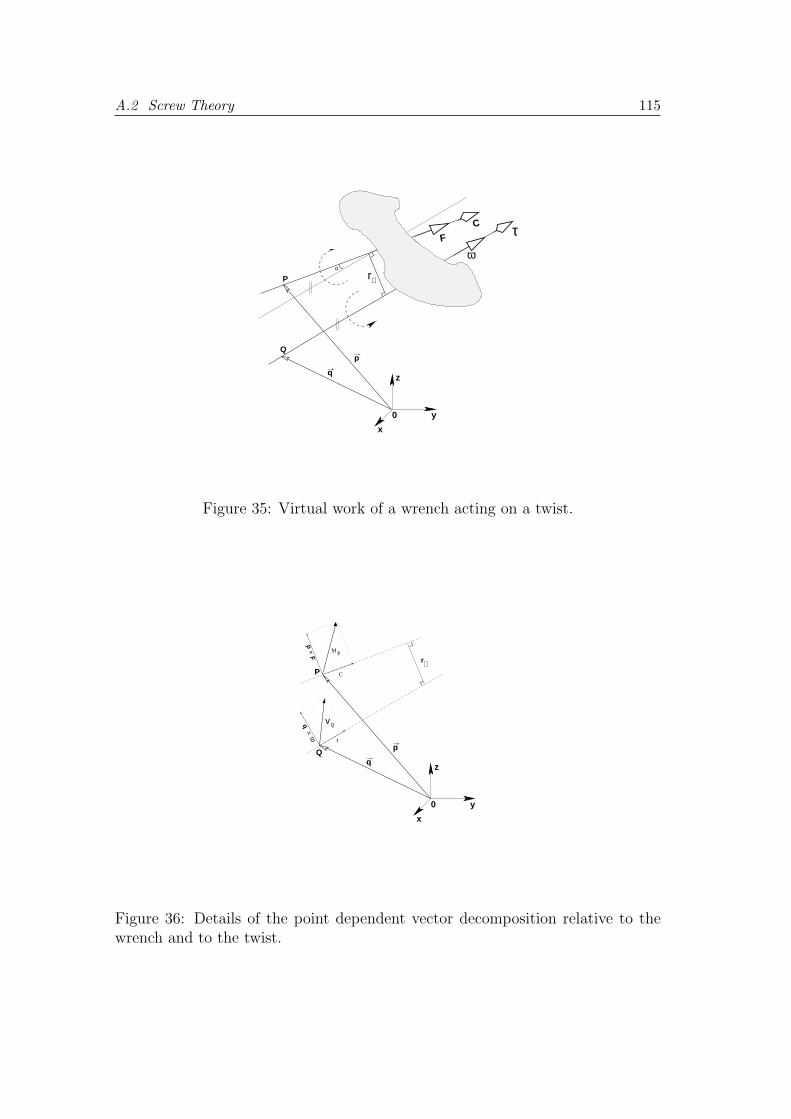
A.2 Screw Theory 115
0
z
y
x
q
p
F
C
P
Q
ω
τ
⊥rα
Figure 35: Virtual work of a wrench acting on a twist.
q
p
pF
×
0
z
y
x
r⊥P C
Q
τ
M P
vQq× ω
Figure 36: Details of the point dependent vector decomposition relative to thewrench and to the twist.

A.2 Screw Theory 116
columns vectors in ray order the eq. (A.15) becomes
W = $waxis$
tray (A.18)
Eq. (A.16) can be interpreted making explicit all combinations of factors that
generate the virtual work in geometrical terms. Quantities are considered along
their respective screw lines. Forces (F) and couples (C) are computed at any point
along the Poinsot’s line and angular velocities ω and translational velocities τ are
computed at any point along the Chasles’ line. Remember that translational
velocity τ coincides with the linear velocity v of any point along the Chasles’
line.
In other words we have two lines: Poinsot’s and Chasles’. At Poinsot’s line
a point is selected and relative to this point we have two parallel vectors (F
and C) acting on the rigid body. On the other side we have a different point
selected at the Chasles’ line with two parallel vectors (ω and τ) representing
completely the rigid body movement. The wrench $w = (F ; C) acts on a body
that instantaneously twists around following $t = (ω; τ). The remaining question
is: What does it mean geometrically the virtual work generated by the wrench $w
acting on the twist $t
F and ω = −Fωr⊥ sin αF and τ = −Fτ cos α = FωhtcosαC and ω = Cω cos α = FωhwcosαC and τ = 0
Table 3: Combination of factors to generate the virtual work
Table 3 lists the virtual work generated by each variable combination. There
r⊥ is the perpendicular distance between Poinsot’s and Chasles’ lines (screw axes),
α is the torsion angle between both axes, ht is the pitch of the twist and hw
is the pitch of the wrench (see Fig. 34). It is worth noticing that both point
independent quantities cannot do any work each other. A couple C can only
impose a rotational “tendency” to the movement of the rigid body and cannot
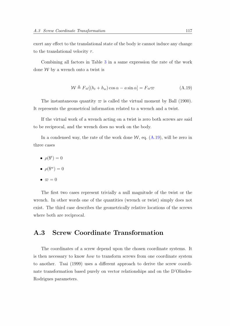
A.3 Screw Coordinate Transformation 117
exert any effect to the translational state of the body ie cannot induce any change
to the translational velocity τ .
Combining all factors in Table 3 in a same expression the rate of the work
done W by a wrench onto a twist is
W , Fω[(ht + hw) cos α− a sin α] = Fω$ (A.19)
The instantaneous quantity $ is called the virtual moment by Ball (1900).
It represents the geometrical information related to a wrench and a twist.
If the virtual work of a wrench acting on a twist is zero both screws are said
to be reciprocal, and the wrench does no work on the body.
In a condensed way, the rate of the work done W , eq. (A.19), will be zero in
three cases
• ρ($t) = 0
• ρ($w) = 0
• $ = 0
The first two cases represent trivially a null magnitude of the twist or the
wrench. In other words one of the quantities (wrench or twist) simply does not
exist. The third case describes the geometrically relative locations of the screws
where both are reciprocal.
A.3 Screw Coordinate Transformation
The coordinates of a screw depend upon the chosen coordinate systems. It
is then necessary to know how to transform screws from one coordinate system
to another. Tsai (1999) uses a different approach to derive the screw coordi-
nate transformation based purely on vector relationships and on the D’Olindes-
Rodrigues parameters.

A.3 Screw Coordinate Transformation 118
A.3.1 Ray-axis screw coordinate transformation
Let us consider first the transformation between ray and axis-coordinates
(section A.2.5) with dual vectors represented as column vectors.
[ω
vP
]ray
=
[03 I3
I3 03
] [vP
ω
]axis
(A.20)
[MP
F
]axis
=
[03 I3
I3 03
] [F
MP
]ray
(A.21)
Eqs. (A.20) and (A.21) are simply permutations among the screw coordinates.
The first three components are changed to the last three components.
The matrix that relates ray and axis-coordinates has some interesting prop-
erties5
∆ =
[03 I3
I3 03
], ∆T = ∆, ∆−1 = ∆ det(∆) = −1 (A.22)
A.3.2 Translation of axes
Another transformation expresses a screw (or screws) in relation to a desired
coordinate system. Let firstly this transformation be a simple translation of
axes. As discussed in section A.2 this transformation does not change the point
independent part of the screw.
In matrix form, the twist transformation in ray-coordinates is
[ω
vQ
]ray
=
[I3 03
SP→Q I3
] [ω
vP
]ray
(A.23)
5Furthermore, ∆ gives an indefinite metric for the space of screws. See proof in [Ciblak1998]. This fact has interesting consequences on the hybrid control problems.

A.3 Screw Coordinate Transformation 119
The matrix SP→Q represents the operator−→QP×. In other words SP→Qx =
−→QP ×x for any six dimensional vector x. The matrix SP→Q is skew-symmetrical.
SP→Q =
0 −xQP yQP
xQP 0 −zQP
−yQP zQP 0
≡ −→QP× (A.24)
where
−→QP = (xQP , yQP , zQP ) = P (xP , yP , zP )−Q(xQ, yQ, zQ)
The transpose of SP→Q is given by
S , SQ→P =
0 −xPQ yPQ
xPQ 0 −zPQ
−yPQ zPQ 0
' −→PQ× (A.25)
where
(xPQ, yPQ, zPQ) = Q(xQ, yQ, zQ)− P (xP , yP , zP )
The matrix TtransQ→P represents a change of origin of the screw representation
without any rotation. In other words TtransQ→P corresponds to a translation of the
coordinate system axes.
TtransQ→P ,
[I3 03
S I3
](A.26)
Naturally
TtransP→Q =
[I3 03
SP→Q I3
]=
[I3 03
−S I3
]
A.3 Screw Coordinate Transformation 120
as the matrix S in eq. (A.25) is skew-symmetrical.
For wrenches in ray-coordinates taken as column vectors similarly
[F
MQ
]ray
=
[I3 03
S I3
] [F
MP
]ray
= TtransP→Q
[F
MP
]ray
(A.27)
For wrenches in axis-coordinates taken as column vectors we have
[MQ
F
]axis
=
[I3 S
03 I3
] [MP
F
]axis
= TtransP→Q
[MP
F
]axis
(A.28)
A.3.3 Rotation of axes
Equations like (A.23) and (A.28) represent the “pointy” variance of the screw
representation. This approach when misused can lead to some conceptual mis-
takes. The whole geometry of the screws is purely line geometry and to restrict
its aspects to points can be sometimes dangerous as pointed out by Hunt (2000).
However the route taken in this section try to explain some frequent doubts for
the screw theory newcomer. One of these questions is: why most treatises related
to screw theory define the Plucker screw coordinates (or the Plucker represen-
tation) of a twist with the linear velocity of the point always instantaneously
coincident with the origin of the coordinate system? When dealing with Statics
we cannot make the summation of forces and couple relatively to any point in
the space? So why this kind of restriction?
The screw can be represented in relation to any point in the space. A triad of
coordinate axes can be attached to this point. These coordinate axes normally are
self intersecting lines mutually orthogonal in the space. The point of intersection
of the three axes is set as the origin of the coordinate system. However this
point (the origin of the coordinate system) need not to be the point where the
summation of forces and couples take place. Naturally a simple translation of
A.3 Screw Coordinate Transformation 121
axes (as discussed in section A.3.2) is enough to conciliate both points: the origin
of the coordinate system and the point where the screw is refereed to.
In section A.3.2 the aspects of the translation of axes in the screw represen-
tation was discussed. Here the effects of a pure rotation of axes are considered.
The next step is the conjugation of both changes of coordinates: first a change
of the origin (pure translation) and then a (pure) rotation of the frame.
Adding an extra rotation of the coordinate system via a rotation matrix R3×3
expresses each one of the dual vectors in a different coordinate system. Matrix
Ri→j is orthogonal and gives the orientation of a free vector specified in frame
i, whose origin is Q, in a second frame j, whose origin is P . The coordinate
system can be conveniently designated by a single number. This number has a
quid pro quo relationship with the label that the rigid body receives during the
robot analysis. For instance it can be 0 for the ground frame up to n for the
end-effector in the Denavit-Hartenberg convention for an n degrees of freedom
manipulator. The effect of Ri→j on the screw coordinates can be expressed by
the block diagonal matrix
Troti→j =
[Ri→j 03
03 Ri→j
](A.29)
The (complete) screw coordinate transformation matrix (Trayi→j) is thus ex-
pressed in ray-coordinates
Trayi→j =
[Ri→j 03
03 Ri→j
] [I3 03
S I3
]=
[Ri→j 03
Ri→jS Ri→j
](A.30)
or in axis-coordinates
Taxisi→j =
[Ri→j 03
03 Ri→j
] [I3 S
03 I3
]=
[Ri→j Ri→jS
03 Ri→j
](A.31)

A.3 Screw Coordinate Transformation 122
The inverse of matrix Trayi→j can be easily derived as
Trayi→j
−1 =
[Ri→j
T ST Ri→jT
03 Ri→jT
]=
[Rj→i −SRj→i
03 Rj→i
](A.32)
Eq. (A.31) consider wrenches as column vectors in axis-coordinates. Wrenches
can be expressed as row vectors in axis coordinates to take advantage of linear
algebra operations. So
Taxisi→j = Taxis
i→j
T=
[Ri→j Ri→jS
03 Ri→j
]T
=
[RT
i→j ST RTi→j
03 RTi→j
]=
[RT
i→j −SRTi→j
03 RTi→j
](A.33)
123
APPENDIX B -- Chasles’ and
Poinsot’s lines
We intend to demonstrate the existence of Chasles’ and Poinsot’s lines by a
vectorial route.. We need first to demonstrate an important lemma, Lemma 10.
The proof follows closely [Ciblak 1998].
The extension of Lemma 10 to Chasles’ or Poinsot’s Theorems is consequence
of the fact that physical quantities in Kinematics or Statics can be represented
by screws.
Firstly, a preliminary historical note: neither Chasles nor Poinsot used screw
theory to prove their theorems. In reality all screw theory was based on the
existence of these theorems as Ball (1900) points out in the introduction of his
treatise. Nevertheless the proofs given here, in reverse chronological order, make
explicit some screw properties and are interesting by themselves.
B.1 Screw independence on representation
Lemma 10 The pitch and screw axis of a screw are independent of the point of
representation.
Proof:
Let P and Q be two arbitrary points at which the screws (represented, for
instance, in ray order) are given by [~aT~bTP ]T and [~aT~bT
Q]T . This proof will be in
B.1 Screw independence on representation 124
two parts. First, it will be shown that the pitch is invariant and then that the
axis is also invariant.
B.1.1 Pitch invariance
From the transformation equation (3.5)
~bQ = ~bP +−→QP × ~a (B.1)
Then by eq. (6.3)
h =~aT~bQ
~aT~a=
~aT~bP
~aT~a+
~aT [−→QP × ~a]
~aT~a=
~aT~bP
~aT~a(B.2)
This confirms that the pitch remains the same after changing the point of repre-
sentation. Using u = a and v = bP eq. (B.2) is the same as eq. (1.2).
B.1.2 Axis invariance
The screw axis, viewed from the coordinate system at P , is a parameterised
line, locus of points pointed by a vector rP . Using eq. (1.3) one possible param-
eterisation is rP (αP ) = αP~a + ~a×~bP
~aT~a. The same line, viewed from the coordinate
system at Q, can be parameterised by rQ(αQ) = αQ~a +~a×~bQ
~aT~a
For the completion of the proof it is only necessary to prove that any point
parameterised at P can be parameterised at Q. In other words for any point on
the screw axis there are αP and αQ such that rP (αP ) and rQ(αQ) locate the same
point.
A geometrical argument is to verify whether the vector triangle rQ =−→QP +rP
is satisfied for every point on the screw axis or not. If this is true so both
B.2 A slightly different approach 125
parameterisation lead to the same line (axis). Expanding−→QP
−→QP = rQ − rP = (αQ − αP )~a +
~a× (~bQ −~bP )
~aT~a(B.3)
Using eq. (B.1) into (B.3)
−→PQ = (αQ − αP )~a +
~a× (−→PQ× ~a)
~aT~a(B.4)
Eq. (B.4) is just a decomposition of vector−→PQ into two components: one par-
allel to and other perpendicular to ~a. Since this is always possible (and unique),
given any αP it is possible to find an αQ such that eq. (B.4) is satisfied uniquely.
Therefore both representations, at P and at Q, result in the same screw axis.
QED
B.2 A slightly different approach
Lemma 10 and the argument developed in section B.1 are enough to prove
Chasles’ or Poinsot’s theorems. Another approach is to use directly the screw
transformation matrices instead. They show the screw coordinates dependence
of the point of representation without considering any rotation of axis.
Both theorems guarantee the existence of a line where the resultant couple
and force (in statics case) or the angular and linear velocities of the points (in
kinematics case) will be parallel.
Another question is about the existence or not of a vector r =−→PQ such that
the screw transformation becomes
[~a
h~a
]ray
=
[I3 03
S I3
] [~a
~bP
]ray
(B.5)
B.2 A slightly different approach 126
Here S ≡ r× as in eq. (4.4).
Eq. (B.5) reduces to a single vector equation
h~a = ~bP + r × a (B.6)
or
~bP = h~a− r × a = h~a− r⊥ × a (B.7)
Observe that
r × a = r⊥ × a
where r⊥ is the vector of minimum length defined in Lemma 10, eq. (1.3).
Equation (B.7) derives from the decomposition of r into components parallel
to ~a (h~a) and components perpendicular to ~a (r⊥ × a)
r =−→PQ = α~a + r⊥ × ~a (B.8)
Decompositions like eq. (B.8) are always possible to be done. Vectors rperp
and a are mutually perpendicular. The curve generated by the tip of vector r
represented by eq. (B.8) is a straight line. This line has α as the free parameter
and ~a/‖~a‖ as it versor. This line is the locus that satisfies the related theorem
(Chasles’ or Poinsot’s). QED

127
APPENDIX C -- Matrix powers
Let Fm×n = Dm×rEr×n be a Boolean matrix F generated by the product of
two generic Boolean matrices D and E. Each element of F is a number 0 or 1
and is generated by the summation
Fi,j =r∑
k=1
Di,k · Ek,j (C.1)
A element Fi,j is null only if all the terms in the summation are zero i.e.
Di,k · Ek,j = 0 ∀k = 1, . . . , r (C.2)
Equations (C.1) and (C.2) can be rewritten in logical (Boolean) terms as
Fi,j = 0 ⇐⇒ Di,k = 0 ∨ Ek,j = 0 ∀k = 1, . . . , r (C.3)
In other words: Fi,j = 1 unless the internal product of row i of first matrix D
with column j of second matrix E is null. This assertion can be explicitly stated
as:
“If there is an arc i → k in the digraph G(D) so there is not an arc k → j in
the digraph G(E) and vice-versa”
A important product of two Boolean matrices is the matrix power i.e. when
D = E in eq. (C.1). Here both matrices represent the same digraph and then
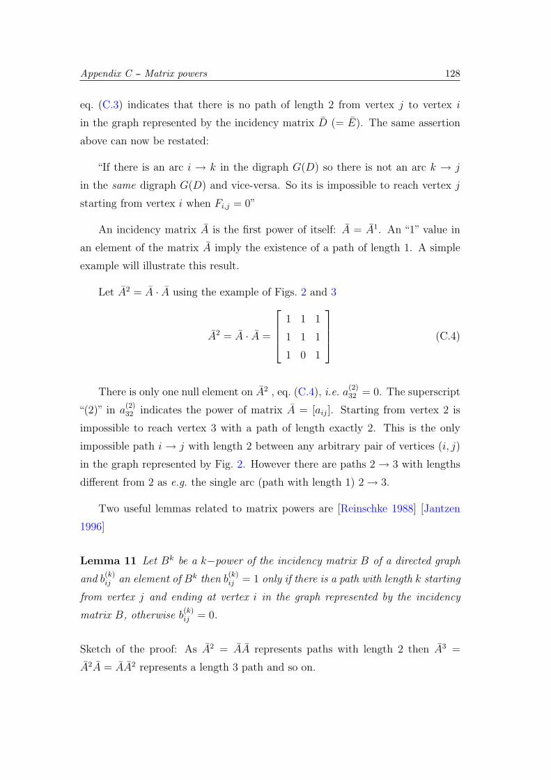
Appendix C -- Matrix powers 128
eq. (C.3) indicates that there is no path of length 2 from vertex j to vertex i
in the graph represented by the incidency matrix D (= E). The same assertion
above can now be restated:
“If there is an arc i → k in the digraph G(D) so there is not an arc k → j
in the same digraph G(D) and vice-versa. So its is impossible to reach vertex j
starting from vertex i when Fi,j = 0”
An incidency matrix A is the first power of itself: A = A1. An “1” value in
an element of the matrix A imply the existence of a path of length 1. A simple
example will illustrate this result.
Let A2 = A · A using the example of Figs. 2 and 3
A2 = A · A =
1 1 1
1 1 1
1 0 1
(C.4)
There is only one null element on A2 , eq. (C.4), i.e. a(2)32 = 0. The superscript
“(2)” in a(2)32 indicates the power of matrix A = [aij]. Starting from vertex 2 is
impossible to reach vertex 3 with a path of length exactly 2. This is the only
impossible path i → j with length 2 between any arbitrary pair of vertices (i, j)
in the graph represented by Fig. 2. However there are paths 2 → 3 with lengths
different from 2 as e.g. the single arc (path with length 1) 2 → 3.
Two useful lemmas related to matrix powers are [Reinschke 1988] [Jantzen
1996]
Lemma 11 Let Bk be a k−power of the incidency matrix B of a directed graph
and b(k)ij an element of Bk then b
(k)ij = 1 only if there is a path with length k starting
from vertex j and ending at vertex i in the graph represented by the incidency
matrix B, otherwise b(k)ij = 0.
Sketch of the proof: As A2 = AA represents paths with length 2 then A3 =
A2A = AA2 represents a length 3 path and so on.
Appendix C -- Matrix powers 129
Another useful Lemma is
Lemma 12 Let Bk be a k−power of the incidency matrix Bn×n of a directed
graph with n vertices. If k ≥ n then Bk will be a full Boolean matrix or will
repeat cyclically the patterns of the powers B1, B2, . . . , Bn−1.
Sketch of the proof: Every path with length greater than or equal to n will
necessarily pass twice by at least one vertex of the graph. If there is such a path
passing through every vertex of the graph then the reachability matrix R is full.
Otherwise, these paths will circulate the strong components of the graph.
Formal proofs of Lemmas 11 and 12 are found in [Reinschke 1988]. The
conjugation of both lemmas above leads to eq. (2.4) which obtains the reachability
matrix from the incidency matrix R =∑n−1
i−1 Ak.

130
APPENDIX D -- Numerical
computation of the
inverse Jacobian
matrix structure
The kinematic structure matrix Qkin depends upon the structure of the Jaco-
bian matrix and its inverse. The Jacobian matrix can be symbolically derived in
a straightforward manner either using Denavit-Hartenberg parameters and their
coordinate systems or using screw theory.
However the symbolic computation of the inverse Jacobian matrix is a tougher
task [Lucas, Tischler e Samuel 2000]. Some hierarchical kinematic analysis advan-
tages, which depends upon the kinematic structure matrix, would be lost if one
must compute Qkin for each robot architecture. Moreover a single robot archi-
tecture can have as many Jacobian matrices as coordinate systems and variables
(angles or lengths) are chosen to describe it.
The efficiency of the analysis of a specific robot architecture is, in a great
extent, a quest for a good coordinate system (possibly the best one) and a corre-
sponding set of descriptor variables that turn the Jacobian as simple as possible.
If, for every trial in the robot analysis, the Jacobian matrix has to be symbolically
inverted the analysis procedure becomes quite cumbersome.
Procedurally Qkin can be expressed only by its structure matrix Qkin i.e. there
is no need to know explicitly the real values of the elements of J and J−1. The
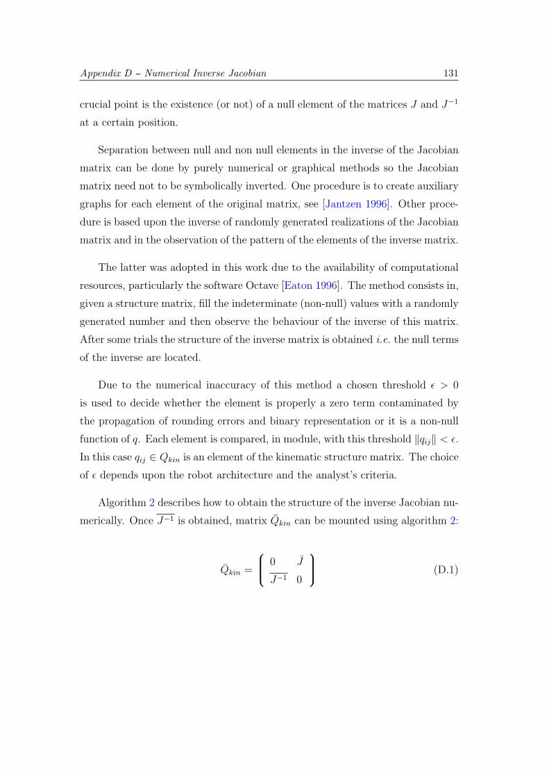
Appendix D -- Numerical Inverse Jacobian 131
crucial point is the existence (or not) of a null element of the matrices J and J−1
at a certain position.
Separation between null and non null elements in the inverse of the Jacobian
matrix can be done by purely numerical or graphical methods so the Jacobian
matrix need not to be symbolically inverted. One procedure is to create auxiliary
graphs for each element of the original matrix, see [Jantzen 1996]. Other proce-
dure is based upon the inverse of randomly generated realizations of the Jacobian
matrix and in the observation of the pattern of the elements of the inverse matrix.
The latter was adopted in this work due to the availability of computational
resources, particularly the software Octave [Eaton 1996]. The method consists in,
given a structure matrix, fill the indeterminate (non-null) values with a randomly
generated number and then observe the behaviour of the inverse of this matrix.
After some trials the structure of the inverse matrix is obtained i.e. the null terms
of the inverse are located.
Due to the numerical inaccuracy of this method a chosen threshold ε > 0
is used to decide whether the element is properly a zero term contaminated by
the propagation of rounding errors and binary representation or it is a non-null
function of q. Each element is compared, in module, with this threshold ‖qij‖ < ε.
In this case qij ∈ Qkin is an element of the kinematic structure matrix. The choice
of ε depends upon the robot architecture and the analyst’s criteria.
Algorithm 2 describes how to obtain the structure of the inverse Jacobian nu-
merically. Once J−1 is obtained, matrix Qkin can be mounted using algorithm 2:
Qkin =
0 J
J−1 0
(D.1)

Appendix D -- Numerical Inverse Jacobian 132
Algorithm 2: Structure of the inverse matrix obtained numericallyAlgorithm: Input data: Jacobian matrix J
1. Extract the structure matrix 〈J〉
2. Compute J = J(q) with arbitrary values for the variables qi, or
3. If J = J(q) is not available,generate a realization J ∈ 〈J〉 with randomvalues
4. Invert J and check the values, in module, with the threshold ε.
5. Repeat items 3, 2 and 4 to confirm the structure matrix of J−1 ie 〈J−1〉

133
APPENDIX E -- Kirchhoff-Davies
circuit law
E.1 Adaptation of the Kirchhoff laws to Kine-
matics
As parallel robots are closed kinematic chains we need to know how to solve
the kinematic problem. The most general technique to solve the kinematics of
closed kinematic chains appears to be the Kirchhoff-Davies laws [Davies 1983]
[Davies 1981] [Davies 1995] [Davies 2000] [Campos 2001], which will be described
in this section.
The Kirchhoff’s circuit law is a fundamental result to solve circuits in electrical
engineering. Davies (1981) adapted this law to the kinematics of closed kinematic
chains, combining graph theory and screw theory. This adaptation solves the set
of instantaneous screws transmitted by independent kinematic pairs to the other
pairs of the chain in a given architecture. The method leads to a matricial
formulation that, additionally, facilitates computational solutions and detects
singularities.
The method is quite general, as it is based on the topology of the kinematic
chain. Kirchhoff-Davies circuit law generates the kinematic matrices by graph
theoretical concepts. The method will be applied to a planar platform with three
degrees of freedom 3RRR.

E.2 Coupling graph of a kinematic chain 134
Initially, the platform kinematics is explained by constructing the coupling
graph of the chain, meanwhile some additional concepts of the theory of graphs
are explained. In the sequence, the movement graph of the kinematic chain is
generated. Finally, by means of the adaptation of the Kirchhoff’s circuit law,
the matrix containing the instantaneous screws of all the kinematic pairs of the
closed chain is calculated.
An additional special terminology described in [Davies 1995] is used to deal
with kinematics chains and graphs.
E.2 Coupling graph of a kinematic chain
The coupling graph GC of a kinematic chain represents each link of the chain
by means of one vertex n (identified by a number) and each kinematic pair of the
chain by means of an edge e (identified by a letter). If an orientation is assigned
to each edge of the graph, we obtain a digraph of the kinematic chain as discussed
in section 2.2.1 and these edges are called arcs. The orientation of the arcs can
be arbitrarily chosen, such as from vertices with lower numbers to vertices with
higher numbers. The mechanism 3RRR in Fig. 37, with n = 8 and e = 9, has an
associated coupling graph shown in Fig. 38.
Some extra concepts of the theory of graphs, not mentioned in Chapter 2,
are here defined, or redefined, in conformity with [Davies 1995]:
• Circuit: a synonym of closed path i.e. a path in which the initial and final
node are the same, see definitions in section 2.2.1 at page 2.2.1.
• Tree: a subgraph which contains all vertices of the graph but no circuits.
A graph can have several associated trees.
Some authors [Harary, Norman e Cartwright 1965] [Tsai 2001] define a tree
as any subgraph containing no circuits. A tree involving all the vertices of
the original graph is, by these authors, called a spanning tree.

E.2 Coupling graph of a kinematic chain 135
2 θF
θH
θE
θB
θA
θG
8
7 1
4
3
5
6
B
CE
I
H
G
D
A Fk
h
�������
����� �������
x
y
Figure 37: Mechanism 3RRR in the xy-plane
3
C
D
I4
5
6
1
A G
8
HB
7
E
F2
Figure 38: Graph of mechanism 3RRR.
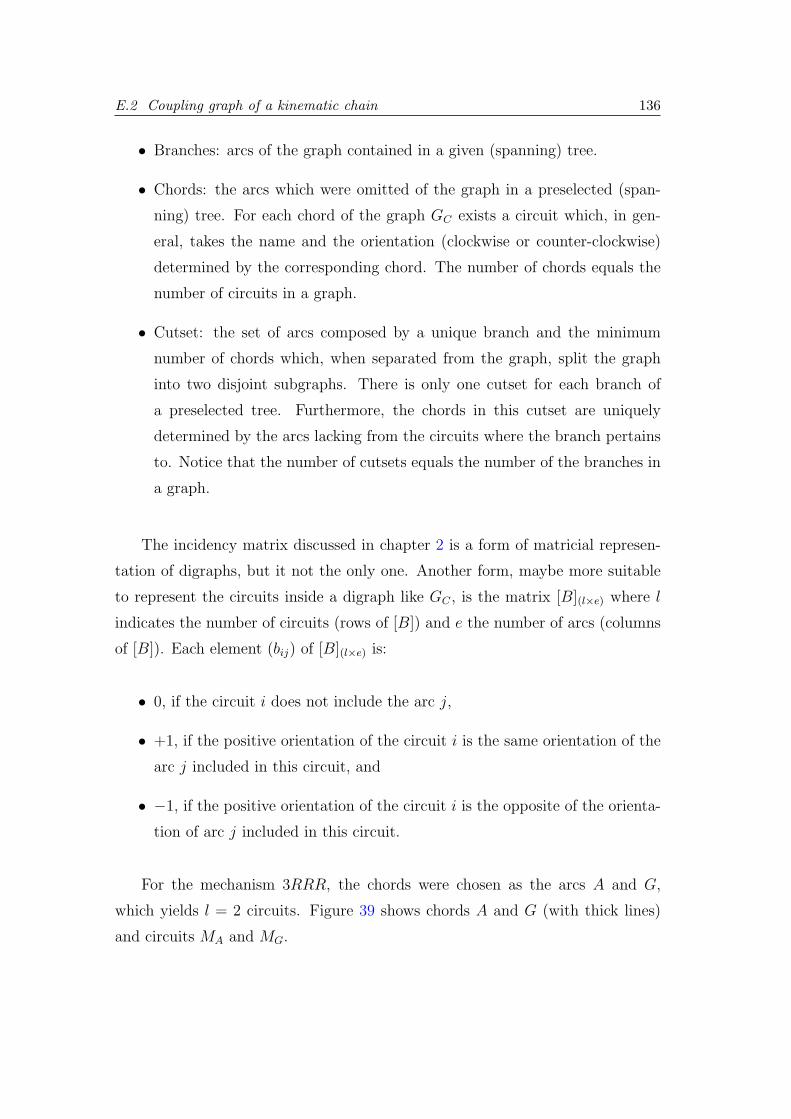
E.2 Coupling graph of a kinematic chain 136
• Branches: arcs of the graph contained in a given (spanning) tree.
• Chords: the arcs which were omitted of the graph in a preselected (span-
ning) tree. For each chord of the graph GC exists a circuit which, in gen-
eral, takes the name and the orientation (clockwise or counter-clockwise)
determined by the corresponding chord. The number of chords equals the
number of circuits in a graph.
• Cutset: the set of arcs composed by a unique branch and the minimum
number of chords which, when separated from the graph, split the graph
into two disjoint subgraphs. There is only one cutset for each branch of
a preselected tree. Furthermore, the chords in this cutset are uniquely
determined by the arcs lacking from the circuits where the branch pertains
to. Notice that the number of cutsets equals the number of the branches in
a graph.
The incidency matrix discussed in chapter 2 is a form of matricial represen-
tation of digraphs, but it not the only one. Another form, maybe more suitable
to represent the circuits inside a digraph like GC , is the matrix [B](l×e) where l
indicates the number of circuits (rows of [B]) and e the number of arcs (columns
of [B]). Each element (bij) of [B](l×e) is:
• 0, if the circuit i does not include the arc j,
• +1, if the positive orientation of the circuit i is the same orientation of the
arc j included in this circuit, and
• −1, if the positive orientation of the circuit i is the opposite of the orienta-
tion of arc j included in this circuit.
For the mechanism 3RRR, the chords were chosen as the arcs A and G,
which yields l = 2 circuits. Figure 39 shows chords A and G (with thick lines)
and circuits MA and MG.

E.3 Movement graph of a kinematic chain 137
3
C
D
I4
5
6
1
A G
8
H
2
B
7
E
F
M MA G
Figure 39: Chords and circuits of the graph GC for the mechanism 3RRR
Thus, the matricial representation of the two circuits MA and MG of GC is:
A B C D E F G H I
B =
[1
0
1
0
1
0
1
−1
1
−1
1
−1
0
1
0
1
0
1
]MA
MG
(E.1)
E.3 Movement graph of a kinematic chain
The movement1 graph GM is a coupling graph where the arcs represent kine-
matic pairs allowing only f = 1 degree of freedom. Thus, each one of the arcs
of GC , representing direct kinematic pairs with f > 1 degrees of freedom, are
substituted by f arcs representing direct kinematic pairs with f = 1 degree of
1While Davies (2000) uses the term motion graph, we adopt here the nomenclature suggestedby Hunt (1978) and corroborated by the Webster’s dictionary which asserts that: Motionexpresses a general idea of not being at rest; movement is oftener used to express a definite,regulated motion, especially a progress.. In this sense, motion could involve e.g. accelerations,inertia factors, etc . . . which were clearly outside the scope of this work.
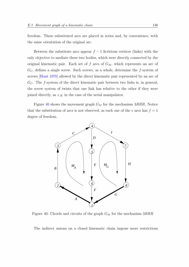
E.3 Movement graph of a kinematic chain 138
freedom. These substituted arcs are placed in series and, by convenience, with
the same orientation of the original arc.
Between the substitute arcs appear f − 1 fictitious vertices (links) with the
only objective to mediate these two bodies, which were directly connected by the
original kinematic pair. Each set of f arcs of GM , which represents an arc of
GC , defines a single screw. Such screws, as a whole, determine the f -system of
screws [Hunt 1978] allowed by the direct kinematic pair represented by an arc of
GC . The f -system of the direct kinematic pair between two links is, in general,
the screw system of twists that one link has relative to the other if they were
joined directly, as e.g. in the case of the serial manipulator.
Figure 40 shows the movement graph GM for the mechanism 3RRR. Notice
that the substitution of arcs is not observed, as each one of the e arcs has f = 1
degree of freedom.
1
2
3
4
5
6
7
8
A
B
CD
E
FG
H
I
M MGA
Figure 40: Chords and circuits of the graph GM for the mechanism 3RRR
The indirect unions on a closed kinematic chain impose more restrictions

E.4 Kirchhoff-Davies circuit law 139
on the movement than the direct kinematic pairs, thus the degree of freedom
f of the directly connected links i and j can be reduced to fij, fij ≤ fi and
fij ≤ fj, due to the presence of the other kinematic pairs. We can define the
gross degree of freedom F of a kinematic chain as the summation F =∑e
1 fi
of all arcs of GM where each arc represents one degree of freedom. For the
mechanism 3RRR the gross degree of freedom is calculated from the kinematic
pairs A, B, C,D,E, F, G, H and I:
F =9∑1
fi =9∑1
1 = 9 (E.2)
Similarly to the graph GC , the graph GM also possesses a matrix which
represents the circuits of the graph: [BM ](l×F ), where F ≤ e, i.e. the number of
arcs in GM cannot be lower than the number of arcs in GC .
Rewriting the matrix [B], but repeating fi times the columns of [B] corre-
sponding to the substituted arcs, leads to a matricial representation [BM ] of the
circuits of GM . For convenience, again, these substituted arcs will keep the same
original of the original arc.
As discussed above, the example discussed here has no kinematic pairs with
fi > 1, and then the matricial representation [BM ] of the circuits of GM is the
same as that of [B]:
A B C D E F G H I
BM = B =
[1
0
1
0
1
0
1
−1
1
−1
1
−1
0
1
0
1
0
1
]MA
MG
(E.3)
E.4 Kirchhoff-Davies circuit law
The Kirchhoff’s circuit law adapted to the kinematic case requires the rela-
tionship of the screws of all the kinematic pairs pertaining to the same circuit.
The basic principle underlining this adaptation is that the movement of a link rel-
atively to itself is always null. Thus, the matrix of the normalised screws (in open

E.4 Kirchhoff-Davies circuit law 140
chain) of the kinematic pairs MD is constrained by the the matrix that relates
the role each link has in each circuit BM . The matrix of normalised screws MN
combines these two aspects of the closed kinematic chains, namely: independent
screws associated with each joint and the closure of the kinematic chain.
Let d (1 ≤ d ≤ 6) be the minimum order of the screw-system (d-system) to
which belong all the F screws of the kinematic chain. So, we generate the matrix
[MD](d×F ) which represents all (normalised) screws of the direct kinematic pairs,
i.e. the screws allowed for each kinematic pair without the restrictions of the
remaining kinematic pairs of the kinematic chain. Each column of [MD](d×F ) is
the normalised screw of an arc of GM (one degree-of-freedom screw).
As the mechanism 3RRR is planar, d = 3, we consider only three Plucker’s
coordinates N ,P and Q [Hunt 1978]. Therefore, the matrix of normalised screws,
where the d rows represent the Plucker’s coordinates and the F columns represent
the instantaneous screw at each kinematic pair of f = 1 degree of freedom, is
given by
MTD =
P Q N
0
psa
qsba + psa
qsfe + psf
psf
0
hk
psg + hk
qshg + psg + hk
0
−pca
−qcba − pca
−qcfe − pcf − k
−pcf − k
−k
−k2
−pcg − k2
−qchg − pcg − k2
1
1
1
1
1
1
1
1
1
A
B
C
D
E
F
G
H
I
(E.4)
where the matrix MD is shown transposed in eq. (E.4) due to space restrictions.
In eq. (E.4) sa = sin θA, sb = sin θB, ca = cos θA, sba = sin(θB+θA), cba = cos(θB+
θA), etc . . . The dimensions p = AB = EF = GH, and q = BC = FG = HI
complete the dimensions shown in Fig. 37.
Matrix MD does not represent the true plot of the movements of the kinematic
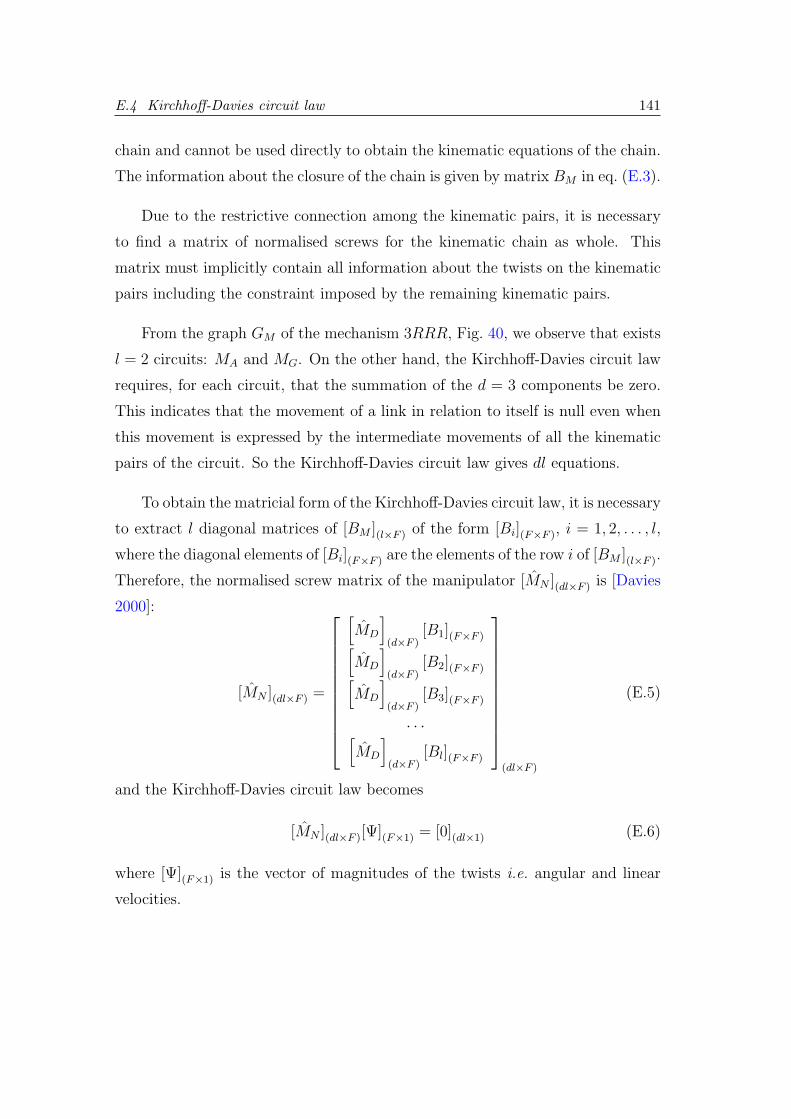
E.4 Kirchhoff-Davies circuit law 141
chain and cannot be used directly to obtain the kinematic equations of the chain.
The information about the closure of the chain is given by matrix BM in eq. (E.3).
Due to the restrictive connection among the kinematic pairs, it is necessary
to find a matrix of normalised screws for the kinematic chain as whole. This
matrix must implicitly contain all information about the twists on the kinematic
pairs including the constraint imposed by the remaining kinematic pairs.
From the graph GM of the mechanism 3RRR, Fig. 40, we observe that exists
l = 2 circuits: MA and MG. On the other hand, the Kirchhoff-Davies circuit law
requires, for each circuit, that the summation of the d = 3 components be zero.
This indicates that the movement of a link in relation to itself is null even when
this movement is expressed by the intermediate movements of all the kinematic
pairs of the circuit. So the Kirchhoff-Davies circuit law gives dl equations.
To obtain the matricial form of the Kirchhoff-Davies circuit law, it is necessary
to extract l diagonal matrices of [BM ](l×F ) of the form [Bi](F×F ), i = 1, 2, . . . , l,
where the diagonal elements of [Bi](F×F ) are the elements of the row i of [BM ](l×F ).
Therefore, the normalised screw matrix of the manipulator [MN ](dl×F ) is [Davies
2000]:
[MN ](dl×F ) =
[MD
](d×F )
[B1](F×F )[MD
](d×F )
[B2](F×F )[MD
](d×F )
[B3](F×F )
· · ·[MD
](d×F )
[Bl](F×F )
(dl×F )
(E.5)
and the Kirchhoff-Davies circuit law becomes
[MN ](dl×F )[Ψ](F×1) = [0](dl×1) (E.6)
where [Ψ](F×1) is the vector of magnitudes of the twists i.e. angular and linear
velocities.
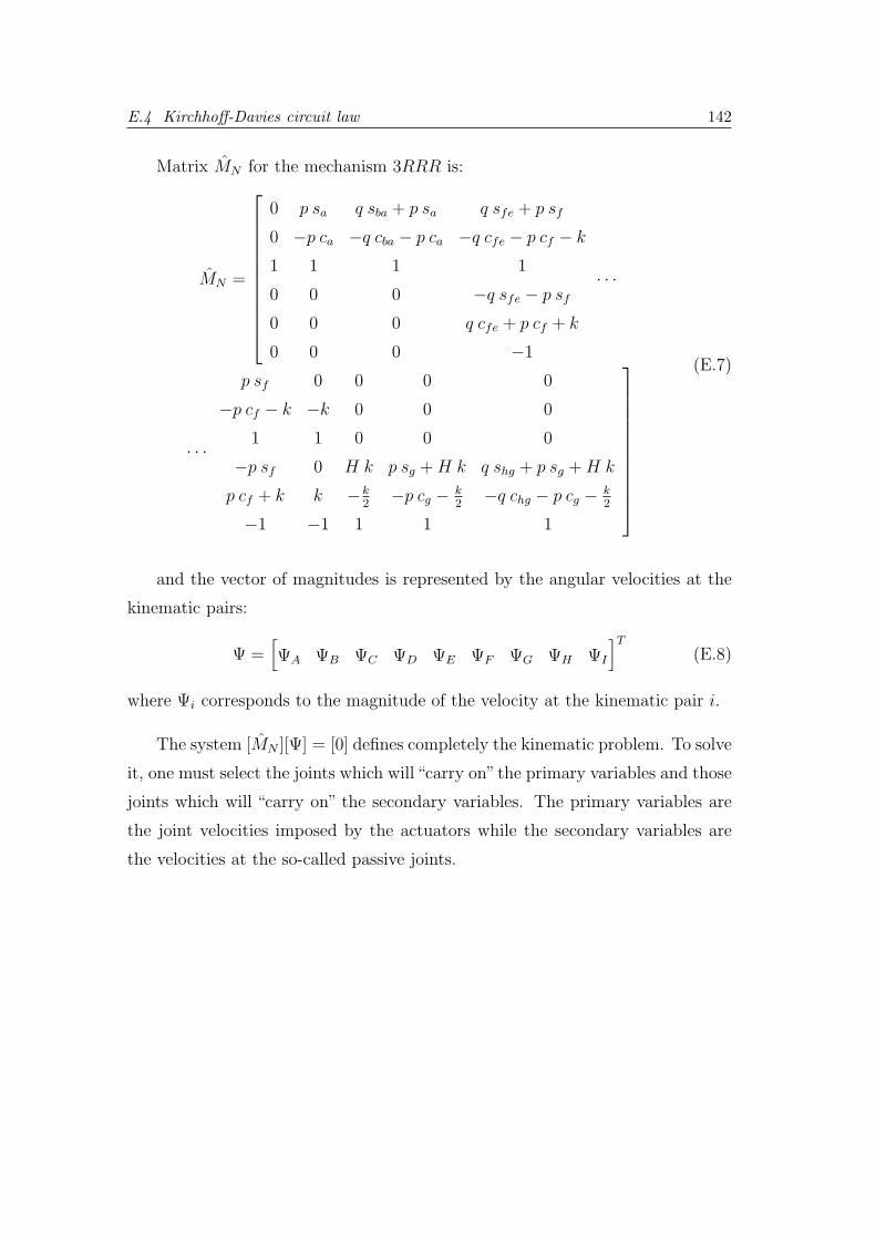
E.4 Kirchhoff-Davies circuit law 142
Matrix MN for the mechanism 3RRR is:
MN =
0 p sa q sba + p sa q sfe + p sf
0 −p ca −q cba − p ca −q cfe − p cf − k
1 1 1 1
0 0 0 −q sfe − p sf
0 0 0 q cfe + p cf + k
0 0 0 −1
· · ·
· · ·
p sf 0 0 0 0
−p cf − k −k 0 0 0
1 1 0 0 0
−p sf 0 H k p sg + H k q shg + p sg + H k
p cf + k k −k2
−p cg − k2
−q chg − p cg − k2
−1 −1 1 1 1
(E.7)
and the vector of magnitudes is represented by the angular velocities at the
kinematic pairs:
Ψ =[ΨA ΨB ΨC ΨD ΨE ΨF ΨG ΨH ΨI
]T
(E.8)
where Ψi corresponds to the magnitude of the velocity at the kinematic pair i.
The system [MN ][Ψ] = [0] defines completely the kinematic problem. To solve
it, one must select the joints which will “carry on”the primary variables and those
joints which will “carry on” the secondary variables. The primary variables are
the joint velocities imposed by the actuators while the secondary variables are
the velocities at the so-called passive joints.

143
References
ANGELES, J. Fundamentals of Robotic Mechanical Systems. New York:Springer, 1997.
ARTOBOLEVSKI, I. I. Teori� mehanizmov i maxin. fourth. Moscow: Nauka,1988. 640 p. In English Mechanism and Machine Theory. ISBN 5-02-013810-X.
ASADA, H.; SLOTINE, J. J. E. Robot Analysis and Control. [S.l.]: John Wileyand Sons, 1986.
ASSUR, L. V. Issledovanie ploskih sternevyh mehanizmov s nizimi parami stoki zreni� ih struktury i klassifikacii. [S.l.]: Izdat. Akad. Nauk SSSR, 1952.592 pp. (4 folded insets, 1 plate) p. Edited by I. I. Artobolevskiı. In EnglishResearch about the structure and classification of plane mechanisms.
BAILLIEUL, J. Kinematic programming alternatives for redundantmanipulators. In: Proc. 1985 IEEE Int. Conf. Robotics & Automation. [S.l.:s.n.], 1985. p. 722–728.
BAKER, D.; WAMPLER, C. The inverse kinematics of redundant manipulators.The International Journal of Robotics Research, v. 7, n. 2, p. 3–21, March/April1988.
BALL, R. S. A Treatise on the Theory of Screws. Cambridge: CambridgeUniversity Press, 1900. ISBN 0521636507 -reedicao 1998.
BARANOV, G. G. Curso de la Teorıa de Mecanismos y Maquinas. second.moscow: mir, 1985. Spanish translation. Russian original.
BOTTEMA, O.; ROTH, B. Theoretical Kinematics. New York: Dover, 1979.
BRUALDI, R. A.; RYSER, H. J. Combinatorial matrix theory. Cambridge[England] ; New York: Cambridge University Press, 1991. ISBN 0521322650.
CAMPOS, A. Calculo da Matriz Cinematica de Rede do Manipulador Paralelo3RRR baseado na Lei de Kirchhoff e na Teoria de Helicoides. Florianopolis, SC,2001.

References 144
CHANG, P. H. A Closed Form Solution for Inverse Kinematics of RobotManipulator with Redundancy. [S.l.], 1986.
CHIAVERINI, S. Singularity-robust task-priority redundancy resolution forreal-time kinematic control of robot manipulators. IEEE Transactions onRobotics and Automation, IEEE, p. 399–410, July 1997.
CIBLAK, N. Analysis of Cartesian Stiffness and Compliance with Applications.Tese (Doutorado) — Georgia Institute of Technology, maio 1998.
COE, C. J. Theoretical mechanics : a vectorial treatment. New York: TheMacmillan, 1938.
CORKE, P. I. A robotics toolbox for MATLAB. IEEE Robotics and AutomationMagazine, v. 3, n. 1, p. 24–32, Mar 1996.
DAVIES, T. The 1887 committee meets again. subject: freedom and constraint.In: HUNT, H. (Ed.). Ball 2000 Conference. Trinity College: CambridgeUniversity Press, 2000. p. 1–56.
DAVIES, T. H. Kirchhoff’s circulation law applied to multi-loop kinematicchains. Mechanism and Machine Theory, v. 16, p. 171–183, 1981.
DAVIES, T. H. Mechanical networks—I: Passivity and redundancy. Mechanismand Machine Theory, v. 18, n. 2, p. 95–101, 1983.
DAVIES, T. H. Mechanical networks—III: Wrenches on circuit screws.Mechanism and Machine Theory, v. 18, n. 2, p. 107–112, 1983.
DAVIES, T. H. Circuit actions attributable to active couplings. Mechanism andMachine Theory, v. 30, n. 7, p. 1001–1012, 1995.
DAVIES, T. H. Couplings,coupling network and their graphs. Mechanism andMachine Theory, v. 30, n. 7, p. 991–1000, 1995.
DENAVIT, J.; HARTENBERG, R. S. A kinematic notation for lower-pairmechanisms based on matrices. Trans. ASME E, Journal of Applied Mechanics,v. 22, p. 215–221, June 1955.
DIMENTBERG, F. M. A general method for the investigation of finitedisplacements of spatial mechanisms and certain cases of passive joints. Akad.Nauk, SSSR Trudi Sem. Teorii Mash. Mekh., v. 5, n. 17, p. 5–39, PurdueTranslation No. 436 1948.
DOTY, K. L.; MELCHIORRI, C.; BONIVENTO, C. A theory of generalizedinverse applied to robotics. Int. J. Robotics Research, v. 12, n. 1, p. 1–19, 1993.
References 145
DUFFY, J. The fallacy of modern hybrid control theory that is based on’orthogonal complements’ of twist and wrench space. Journal of Robotic Systems,v. 7, n. 2, p. 139–144, 1990.
EATON, J. W. Octave: A High Level Interactive Language for NumericalComputations. Second. [S.l.], October 1996. For Octave Version 1.94.
FANGHELLA, P.; GALLETTI, C. Kinematics of robot mechanisms with closedactuating loops. International Journal of Robotics Research, v. 9, n. 6, p. 19–24,Dec 1990.
FANGUELLA, P. Kinematics of single-loop mechanisms and serial robot arms:A systematic approach. Meccanica, v. 30, p. 685–705, 1995.
FANGUELLA, P.; GALLETTI, C. Particular or general methods in robotkinematics. Mechanism and Machine Theory, v. 24, n. 5, p. 383–394, 1989.
GIBSON, C. G.; HUNT, K. H. Geometry of screws systems parts 1 and 2.Mechanism and Machine Theory, v. 25, n. 1, p. 1–27, 1990.
GOLUB, G. H.; LOAN, C. F. van. Matrix Computations. [S.l.]: North OxfordAcademic Publishing, 1983.
GOSSELIN, C. M. Kinematische und statische analyse eines ebenen parallelenmanipulators mit dem freihaitsgrad zwei. Mechanism and Machine Theory,v. 31, n. 2, p. 149–160, 1996.
GOSSELIN, C. M.; MERLET, J.-P. The direct kinematics of planar parallelmanipulators: Special architectures and number of solutions. Mechanism andMachine Theory, v. 29, n. 8, p. 1083–1097, 1994.
GOUGH, V. E.; WHITEHALL, S. G. Universal tyre testing machine. In:F.I.S.I.T.A, INSTITUTION OF MECHANICAL ENGINEERS. Proceedings ofthe 9th International Technical Congress. London, 1962.
GUENTHER, R.; SIMAS, H.; PIERI, E. R. de. Concepcao cinematica deum manipulador para volumes de trabalho restritos. In: Proceedings of theCongresso Nacional de Engenharia Mecanica. [S.l.: s.n.], 2000. in CDROM. InEnglish : Kinematic conception of a manipulator for constrained workspaces.
HARARY, F. (Ed.). Graph Theory and Theoretical Physics. London: AcademicPress, 1967.
HARARY, F.; NORMAN, R. Z.; CARTWRIGHT, D. Structural Models: AnIntroduction to the Theory of Directed Graphs. 4. ed. New York: John Wiley &Sons, 1965.

References 146
HARTENBERG, R. S.; DENAVIT, J. Kinematic Synthesis of Linkages. NewYork: McGraw-Hill, 1964.
HOLLERBACH, J. M. Optimum kinematic design for a seven degree of freedommanipulator. In: HANAFUSA, H.; INOUE, H. (Ed.). Robotics Research 2ndInternational Symposium. Kyoto, Japan: MIT Press, 1985. p. 215–222.
HU, Y.-R.; GOLDENBERG, A. A. An adaptive approach to motion and forcecontrol of multiple coordinated manipulators. Journal of Dynamic Systems,Measurement, and Control, v. 115, p. 60–69, 1993.
HU, Y.-R.; VUKOVICH, G. Dynamic control of free-floating coordinated spacerobots. Journal of Robotic Systems, v. 15, n. 4, p. 217–230, 1998.
HUNT, K. H. Kinematic Geometry of Mechanisms. Oxford: Clarendon Press,1978.
HUNT, K. H. Structural kinematics of in-parallel-actuated robot-arms. Trans.ASME, Journal of Mechanisms, Transmissions and Automation in Design,v. 105, p. 705–712, Dec 1983.
HUNT, K. H. Robot kinematics—a compact analytic inverse solutionfor velocities. Trans. ASME, Journal of Mechanisms, Transmissions andAutomation in Design, v. 109, p. 42–49, March 1987.
HUNT, K. H. Dont’t cross-thread the screw. In: HUNT, H. (Ed.). Ball 2000Conference. Trinity College: Cambridge University Press, 2000. p. 1–37.
HUNT, K. H.; MCAREE, P. R. The octahedral manipulator: Geometry andmobility. International Journal of Robotics Research, v. 17, n. 8, p. 868–885,1998.
INNOCENTI, C. Polynominal solution to the position analysis of the 7-linkassur kinematic chain with one quaternary link. Mechanism and MachineTheory, v. 30, n. 8, p. 1295–1303, 1995.
JANTZEN, J. Digraph Analyses of Linear Control Systems. Dept of Automation:Technical University of Denmark, 1996. Publ. 96-H-838 (lecture notes).
JR, M. B. L.; NUGENT, L. M.; SARIDIS, G. N. Efficient PUMA manipulatorJacobian calculation and inversion. Journal of Robotic Systems, v. 4, n. 2, p.185–197, 1987.
KATZ, A. Computational Rigid Vehicle Dynamics. first. Malabar, Florida, USA:Krieger Publisher Company, 1997.
References 147
KLEIN, C.; CHU-JENQ, C.; AHMED, S. Use of an extended jacobian methodto map algorithmic singularities. In: Werner, Robert; O’Conner, L. (Ed.).Proceedings of the 1993 IEEE International Conference on Robotics andAutomation: Volume 3. Atlanta, GE: IEEE Computer Society Press, 1993. p.632–637. ISBN 0-8186-3450-2.
KLEIN, C.; CHU-JENQ, C.; AHMED, S. A new formulation of the extendedJacobian method and its use in mapping algorithmic singularities forkinematically redundant manipulators. 1995.
KLEIN, C. A.; HUANG, C. H. Review of pseudoinverse control for use withkinematically redundant manipulators. IEEE Transactions on Systems Man andCybernetics, v. 13, n. 3, p. 245–250, 1983.
KU, D.-M. Direct displacement analysis of a Stewart platform mechanism.Mech. Mach. Theory, v. 34, n. 3, p. 453–465, 1999.
LUCAS, S. R.; TISCHLER, C. R.; SAMUEL, A. E. Real-time solution of theinverse kinematic-rate problem. International Journal of Robotics Research,v. 19, n. 12, p. 1236–1244, December 2000.
MANOLESCU, N. I. For a united point of view in the study of the structuralanalysis of kinematic chains and mechanisms. Journal of Mechanisms, v. 3, p.149–169, 1968.
MANOLESCU, N. I.; MANAFU, V. Sur la determination du degre de mobilitedes mecanismes. Bull Polytech. Inst. Bucharest, v. 25, p. 45–66, 1963.
MARTINS, D. Geometrical and Combinatorial Approaches to Robot ManipulatorsKinematics. Florianopolis, SC, 2000.
MARTINS, D.; GUENTHER, R. Hierarchical singularity analysis of anarticulated robot. In: Proceedings of the Brazilian Congress of MechanicalEngineering -IX COBEM. Uberlandia: Brazilian Society of Mechanical Sciences,2001. p. ??–??
MARTINS, D.; GUENTHER, R. Hierarchical singularity analysis of robots. In:ESPINDOLA, J. J.; LOPES, E. M. O.; BAZAN, F. S. V. (Ed.). Proceedings ofthe Nineth International Symposium on Dinamic Problems in Mechanics -IXDINAME. Florianopolis: Brazilian Society of Mechanical Sciences, 2001. p.219–224. ISBN 85-85769-05-X.
MARTINS, D.; MACIE, C. A. Sistematica computacional para a resolucao degrupos de Assur de segunda ordem. In: MACHADO, R. D. (Ed.). Anais do XIVCILAMCE -Congresso Ibero-Latino-Americano de Metodos Computacionais emEngenharia. [S.l.], 1995. v. 2. In Portuguese.

References 148
MARTINS, D.; MACIE, C. A. Determinacao de reacoes em grupos de Assurde primeira ordem. In: UNIVERSIDAD DE VALDIVIA. Congreso NacionalChileno de Ingenierıa. Valdivia, Chile, 1996.
MARTINS, D.; MACIE, C. A. Determinacao de reacoes em grupos de Assurde primeira ordem. In: UNIVERSIDAD DE VALDIVIA. Congreso NacionalChileno de Ingenierıa. Valdivia, Chile, 1996.
MARTINS, D.; SIMAS, H.; GUENTHER, R. Singularity avoidance based on theglobally constrained Jacobian method. Florianopolis, SC, 2001. In Portuguese.
MOZZI, G. Discorso matematico sopra il rotamiento momentaneo dei corpi.naples: Stamperia di Donato Campo, 1763.
MUROTA, K. Systems analysis by graphs and matroids: Structural solvabilityand controllability. Berlin: Springer-Verlag, 1987. ISBN 3-540-17659-4.
MUROTA, K. Matrices and Matroids for Systems Analysis. Berlin: Springer-Verlag, 2000. ISBN 3540660240.
MUROTA, K.; SCHARBRODT, M. Computing the combinatorial canonicalform of a layered mixed matrix. Optimization Methods and Software, v. 10, n. 2,p. 373–391, 1998.
MURRAY, R. M.; LI, Z.; SASTRY, S. S. A Mathematical Introduction toRobotic Manipulation. Ann Arbor: CRC Press, 1994.
NAKAMURA, Y.; HANAFUSA, H. Inverse kinematic solutions with singularityrobustness for robot manipulator control. Journal of Dynamic Systems,Measurement and Control, v. 108, p. 163–171, September 1986.
NENCHEV, D. N. Redundancy resolution through local optimization: A review.J. Robot. Syst., v. 6, n. 6, p. 769–798, December 1989.
ORWANT, J.; HIETANIEMI, J.; MACDONALD, J. Mastering Algorithms withPerl. [S.l.]: O’Reilly & Associates, 1999. ISBN 1-56592-398-7.
PARENTI-CASTELLI, V.; GREGORIO, R. D. Closed-form solution of thedirect kinematics of the 6-3 type stewart platform using one extra sensor.Meccanica, v. 31, n. 6, p. 705–714, 1996.
PARK, J.; CHUNG, W. K.; YOUM, Y. Behaviors of extended jacobian methodfor kinematic resolutions of redundancy. In: STRAUB, E.; SIPPLE, R. S.(Ed.). Proceedings of the International Conference on Robotics and Automation.Volume 1. Los Alamitos, CA, USA: IEEE Computer Society Press, 1994. p.89–95. ISBN 0-8186-6061-9.

References 149
PHILLIPS, J. Freedom in Machinery, Vol 1. Cambridgeshire: CambridgeUniversity Press, 1984.
PHILLIPS, J. Freedom in Machinery, Vol 2. Cambridgeshire: CambridgeUniversity Press, 1990.
PISSANETSKY, S. Sparse Matrix Technology. New York, NY, USA: AcademicPress, 1984. xiii + 321 p. ISBN 0-12-557580-7.
PLuCKER, J. On a new geometry of space. Phil. Trans., v. 155, p. 725–791,1865.
POINSOT, L. Sur la composition des moments et la composition des aires. J.Ec Polyt. Paris, v. 6, p. 182–205, 1806.
REINSCHKE, K. J. Multivariable control : a graph-theoretic approach. Berlin:Springer-Verlag, 1988. ISBN 0387188991.
SCHENDEL, U. Sparse matrices : numerical aspects with applications forscientists and engineers. Chichester : New York: Ellis Horwood ; Halsted Press,1989. ISBN 074580635X.
SCIAVICCO, L.; SICILIANO, B. Modeling and Control of Robot Manipulators.[S.l.]: McGraw-Hill, 1996. (Electrical and Computer Engineering). ISBN0070572178.
SELIG, J. M. Geometrical Methods in Robotics. [S.l.]: Springer-Verlag, 1996.
SEMPLE, J. G.; KNEEBONE, G. T. Algebraic Projective Geometry. [S.l.: s.n.],1952.
SESHU, S.; REED, M. B. Linear Graphs and Electrical Networks. Reading:Addison-Wesley, 1961.
SICILIANO, B. Closed-loop inverse kinematics algorithms for redundantspacecraft/manipulator systems. In: Werner, Robert; O’Conner, L. (Ed.).Proceedings of the 1993 IEEE International Conference on Robotics andAutomation: Volume 3. Atlanta, GE: IEEE Computer Society Press, 1993. p.95–100. ISBN 0-8186-3450-2.
SPONG, M. W.; VIDYASAGAR, M. Robot Dynamics and Control. New York:John Wiley and Sons, 1989.
STEWART, D. A platform with six degrees of freedom. Proceedings of theInstitution of Mechanical Engineers, v. 180, n. 15, p. 371–386, 1966.

References 150
TAHMASEBI, F. Kinematic Synthesis and Analysis of a Novel Class ofSix-DOF Parallel Minimanipulators. Tese (Doutorado) — The University ofMaryland, 1992.
TISCHLER, C. Alternative Structures for Robot Hands. Tese (Doutorado) —The University of Melbourne, Melbourne, 1995.
TISCHLER, C. R. Alternative Structures for Robot Hands. Tese (Ph.D.Dissertation) — University of Melbourne, 1995.
TISCHLER, C. R.; HUNT, K. H.; SAMUEL, A. E. On optimizing the kinematicgeometry of a dextrous robot finger. International Journal of Robotics Research,v. 17, p. 1055–1067, 1998.
TISCHLER, C. R. et al. Screw geometry and Ball’s inertia. In: LIPKIN,H.; DUFFY, J. (Ed.). Ball 2000 Conference. Trinity College: University ofCambridge CDROM, 2000. p. 1–14:Ball2000–28.pdf.
TISCHLER, C. R.; SAMUEL, A. E.; HUNT, K. H. Kinematic chains for robothands: Part 1 orderly number-synthesis. Mechanism and Machine Theory, v. 30,n. 8, p. 1193–1215, 1995.
TISCHLER, C. R.; SAMUEL, A. E.; HUNT, K. H. Kinematic chains for robothands: Part 2 kinematic constraints, classification, connectivity, and actuation.Mechanism and Machine Theory, v. 30, n. 8, p. 1217–1239, 1995.
TISCHLER, C. R.; SAMUEL, A. E.; HUNT, K. H. Dextrous robot fingers withdesirable kinematic forms. International Journal of Robotics Research, v. 17, p.996–1012, 1998.
TREVELYAN, J. P. Robots for shearing sheep : shear magic. Oxford ; NewYork: Oxford University Press
”1992. ISBN 0198562527.
TREVELYAN, J. P.; KOVESI, P. D.; ONG, M. C. H. Motion control for a sheepshearing robot. In: Robotics Research. [S.l.: s.n.], 1983. p. 175–190.
TSAI, L.-W. Robot Analysis: the Mechanics of serial and parallel manipulators.New York: John Wiley & Sons, 1999. ISBN 0-471-32593-7.
TSAI, L.-W. Mechanism Design: Enumeration of Kinematic StructuresAccording to Function. Boca Raton: CRC Press, 2001. ISBN 0-8493-0901-8.
VALDIERO, A. C. et al. Calculo e analise do jacobiano de um manipuladorparalelo de 3 graus de liberdade baseado na teoria dos helicoides. In: Proceedingsof the Brazilian Congress of Mechanical Engineering -IX COBEM. Uberlandia:Brazilian Society of Mechanical Sciences, 2001.

References 151
WALDRON, K. J.; WANG, S. L.; BOLIN, S. J. A study of the Jacobian matrixof serial manipulators. Trans. ASME, Journal of Mechanisms, Transmissionsand Automation in Design, v. 107, p. 230–238, 1985.
WANG, S.-L.; WALDRON, K. J. A study of the singular configurations ofserial manipulators. Journal of Mechanisms, Transmissions, and Automation inDesign, v. 109, p. 14–20, 1987.
WOO, L.; FREUDENSTEIN, F. Application of line geometry to theoreticalkinematics and the kinematic analysis of mechanical systems. Journal ofMechanisms, v. 5, p. 417–460, 1970.
WU, W.; HUANG, Y. The direct kinematic solution of the planar Stewartplatform with coplanar ground points. J. Comput. Math., v. 14, n. 3, p. 263–272,1996.
ZABLONSKI, K. I.; BELOKONEV, I. M.; TCHEKIN, B. Teoria de Mecanismose Maquinas. Kiev, Ucrania: Edicoes Ensino Superior, 1989. Em russo.
ZHANG, C.-d.; SONG, S.-M. Forward kinematics of a class of parallel (stewart)platforms with closed-form solutions. J. Rob. Syst., v. 9, n. 1, p. 93–112, 1992.
ZOMAYA, A. Y.; SMITH, H.; OLARIU, S. Computing robot Jacobian onmeshes with multiple buses. Microprocessors and Microsystems, v. 23, p.309–324, 1999.