Embed Size (px)
Citation preview
Elasticity of Demand
Chapter 5
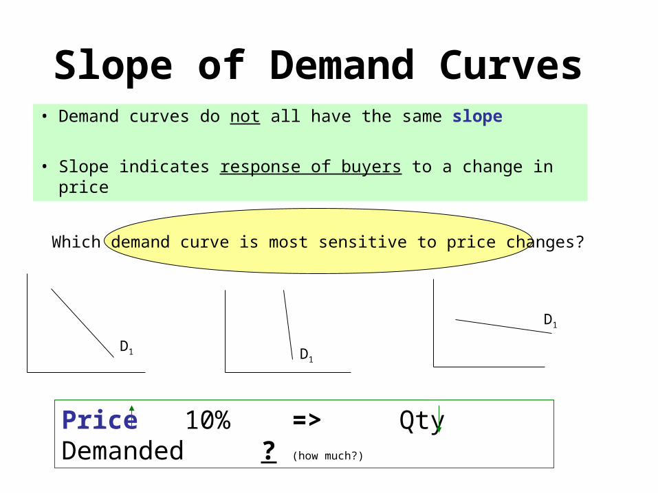
Slope of Demand Curves• Demand curves do not all have the same slope
• Slope indicates response of buyers to a change in price
D1
D1
D1
Price 10% => Qty Demanded ? (how much?)
Which demand curve is most sensitive to price changes?
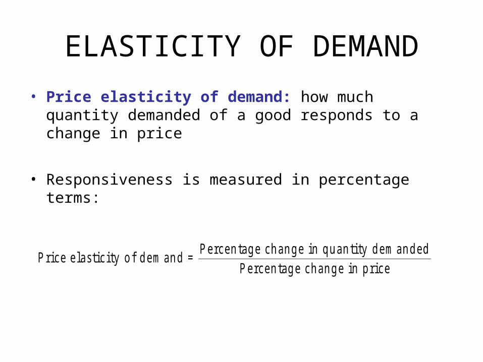
ELASTICITY OF DEMAND
• Price elasticity of demand: how much quantity demanded of a good responds to a change in price
• Responsiveness is measured in percentage terms:
P rice e las tic ity o f d em an d =P ercen tag e ch an g e in q u an tity d em an d ed
P ercen tag e ch an g e in p rice
Determinants of Elasticity of Demand
• Availability of Close Substitutes
• Necessities versus Luxuries
• Proportion of Income
• Time Horizon
Demand is more elastic:
• the larger the number of close substitutes
• if the good is a luxury
• Good is a larger percent of budget
• the longer the time period
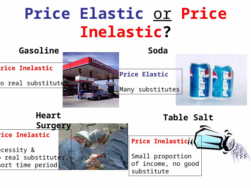
Price Elastic or Price Inelastic?
Soda
Heart Surgery Table Salt
Gasoline
Price Inelastic
No real substitutes
Price Inelastic
Necessity &No real substitutes,Short time period
Price Elastic
Many substitutes
Price Inelastic
Small proportionof income, no goodsubstitute
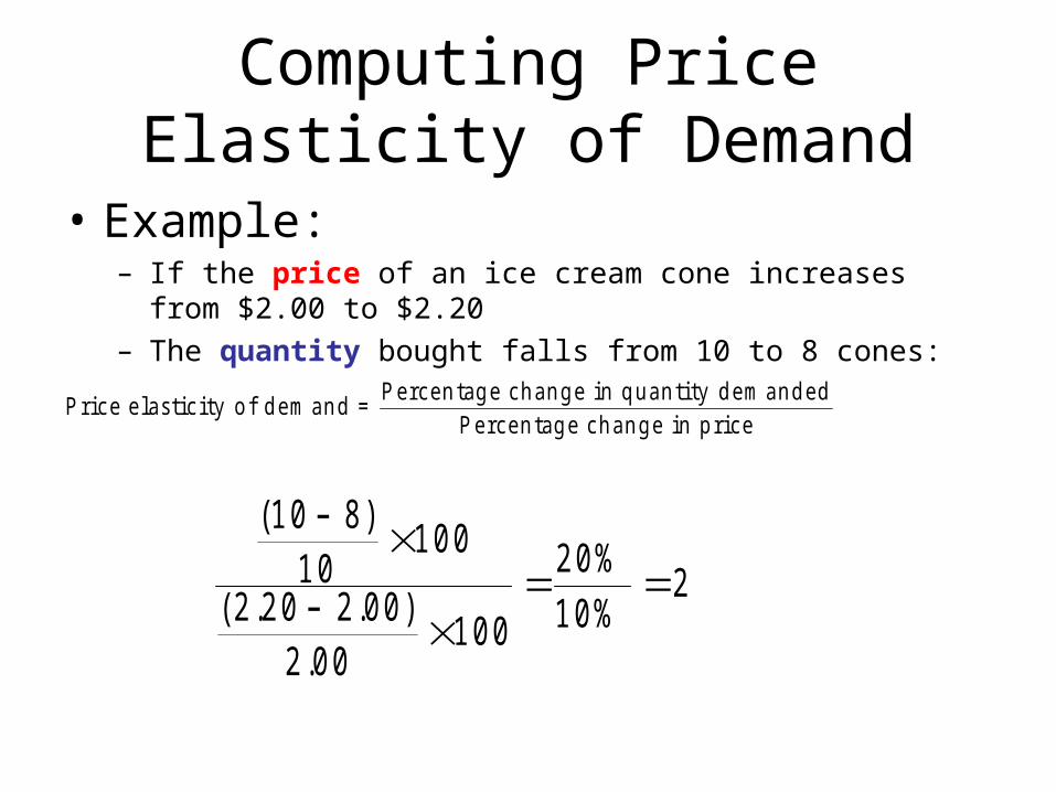
Computing Price Elasticity of Demand
• Example: – If the price of an ice cream cone increases from $2.00 to $2.20 – The quantity bought falls from 10 to 8 cones:
( )
( . . ).
1 0 81 0
1 0 0
2 2 0 2 0 02 0 0
1 0 0
2 0 %
1 0 %2
P rice e las tic ity o f d em an d =P ercen tag e ch an g e in q u an tity d em an d ed
P ercen tag e ch an g e in p rice
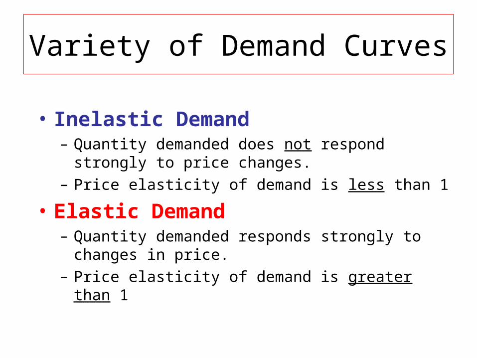
Variety of Demand Curves
• Inelastic Demand– Quantity demanded does not respond strongly to
price changes.– Price elasticity of demand is less than 1
• Elastic Demand– Quantity demanded responds strongly to changes in
price.– Price elasticity of demand is greater than 1
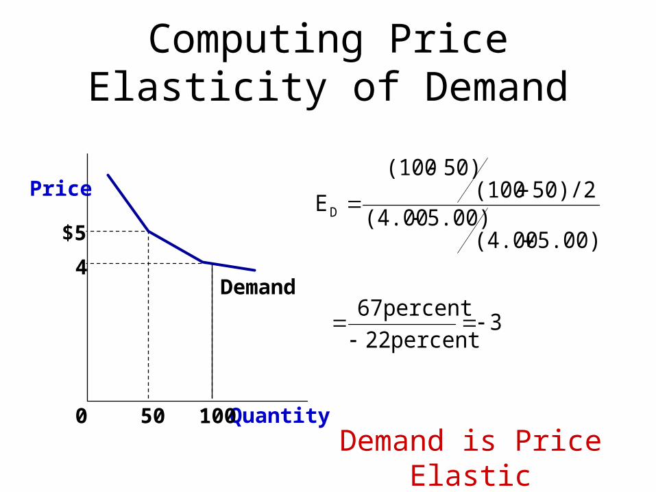
Computing Price Elasticity of Demand
Demand is Price Elastic or Greater than 1---(use absolute values)
$5
4Demand
Quantity1000 50
3percent 22
percent 67
5.00)/2(4.005.00)(4.00
50)/2(10050)(100
ED
Price
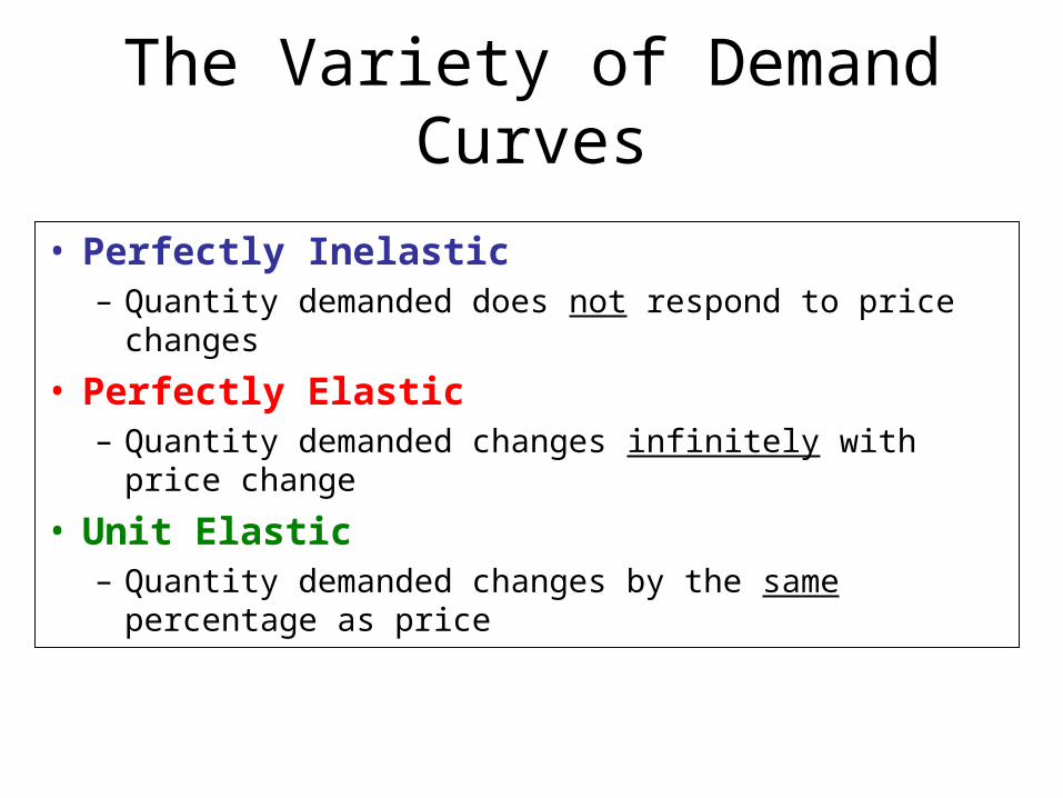
The Variety of Demand Curves
• Perfectly Inelastic– Quantity demanded does not respond to price changes
• Perfectly Elastic– Quantity demanded changes infinitely with price change
• Unit Elastic– Quantity demanded changes by the same percentage
as price
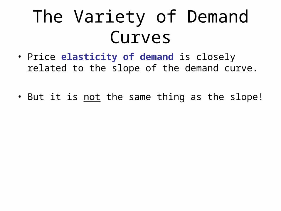
The Variety of Demand Curves
• Price elasticity of demand is closely related to the slope of the demand curve.
• But it is not the same thing as the slope!
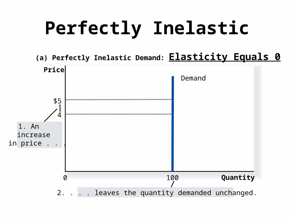
Perfectly Inelastic
(a) Perfectly Inelastic Demand: Elasticity Equals 0
$5
4
Quantity
Demand
1000
1. Anincreasein price . . .
2. . . . leaves the quantity demanded unchanged.
Price
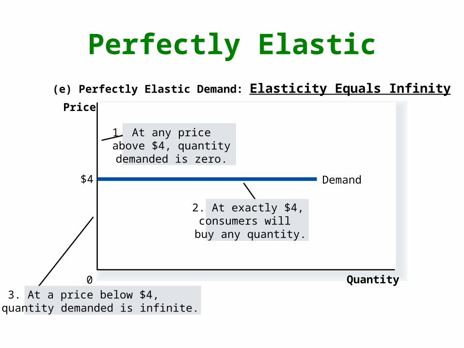
Perfectly Elastic(e) Perfectly Elastic Demand: Elasticity Equals Infinity
Quantity0
Price
$4 Demand
2. At exactly $4,consumers willbuy any quantity.
1. At any priceabove $4, quantitydemanded is zero.
3. At a price below $4,quantity demanded is infinite.
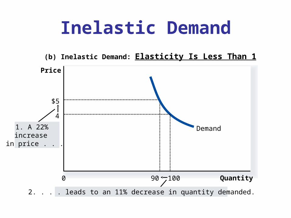
Inelastic Demand
(b) Inelastic Demand: Elasticity Is Less Than 1
Quantity0
$5
90
Demand1. A 22%increasein price . . .
Price
2. . . . leads to an 11% decrease in quantity demanded.
4
100
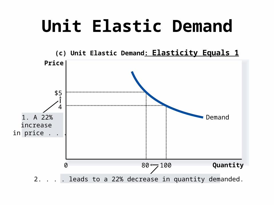
Unit Elastic Demand
2. . . . leads to a 22% decrease in quantity demanded.
(c) Unit Elastic Demand: Elasticity Equals 1
Quantity
4
1000
Price
$5
80
1. A 22%increasein price . . .
Demand
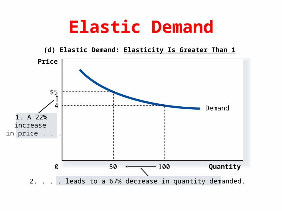
Elastic Demand(d) Elastic Demand: Elasticity Is Greater Than 1
Demand
Quantity
4
1000
Price
$5
50
1. A 22%increasein price . . .
2. . . . leads to a 67% decrease in quantity demanded.
Elasticity & Total Revenue
Chapter 5
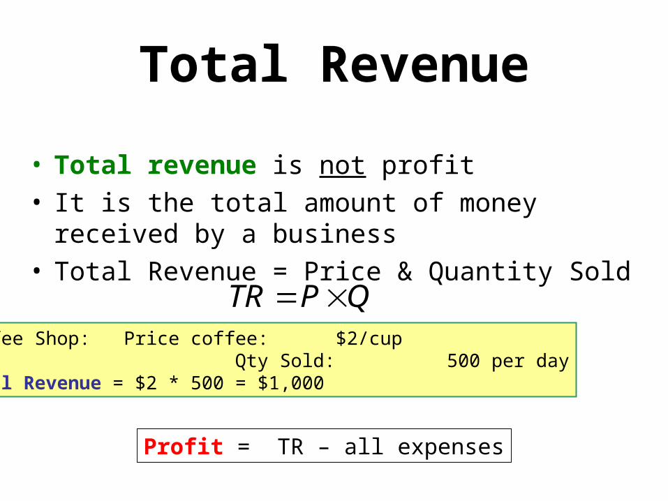
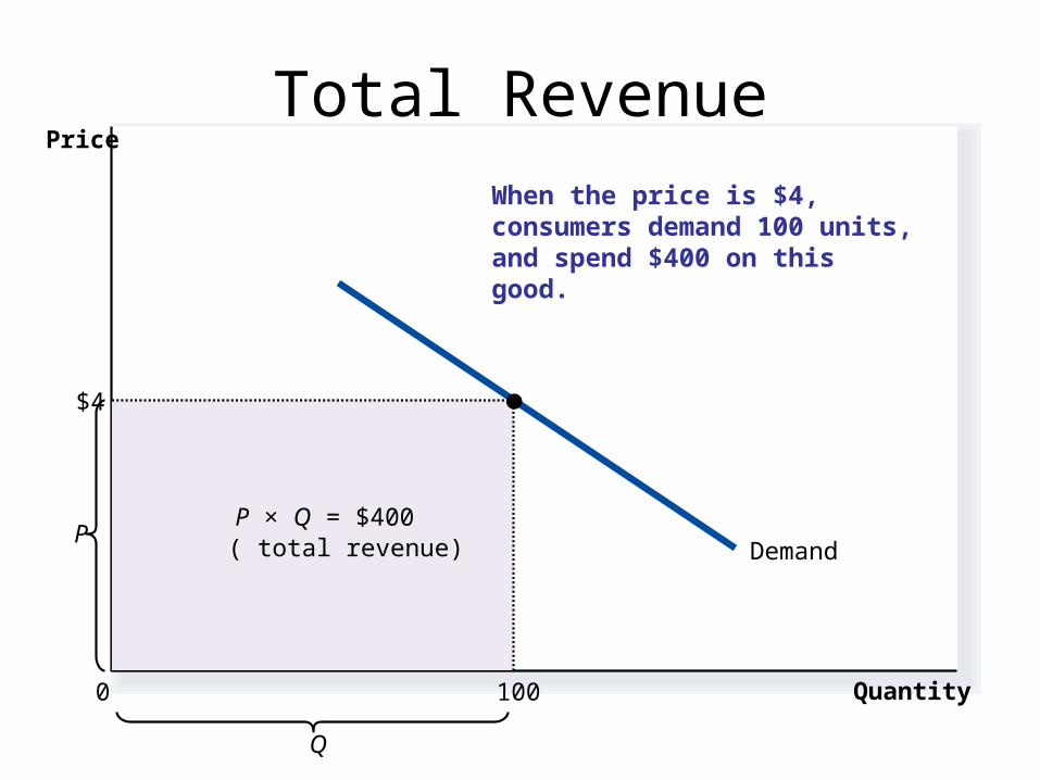
Total Revenue
• Total revenue is not profit• It is the total amount of money received by a
business• Total Revenue = Price & Quantity Sold
QPTR Coffee Shop: Price coffee: $2/cup Qty Sold: 500 per dayTotal Revenue = $2 * 500 = $1,000
Profit = TR – all expenses
Total Revenue
Demand
Quantity
Q
P
0
Price
P × Q = $400( total revenue)
$4
100
When the price is $4, consumers demand 100 units, and spend $400 on this good.
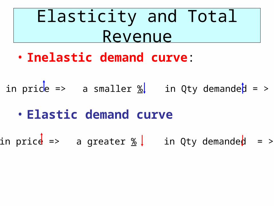
Elasticity and Total Revenue
• Inelastic demand curve:
• Elastic demand curve
in price => a smaller % in Qty demanded = > TR
in price => a greater % in Qty demanded = > TR
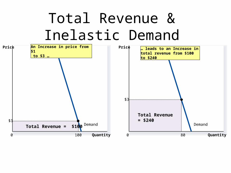
Total Revenue & Inelastic Demand
Demand
Quantity0
Price
Total Revenue = $100
Quantity0
Price
Total Revenue = $240
Demand$1
100
$3
80
An Increase in price from $1 to $3 …
… leads to an Increase in total revenue from $100 to $240
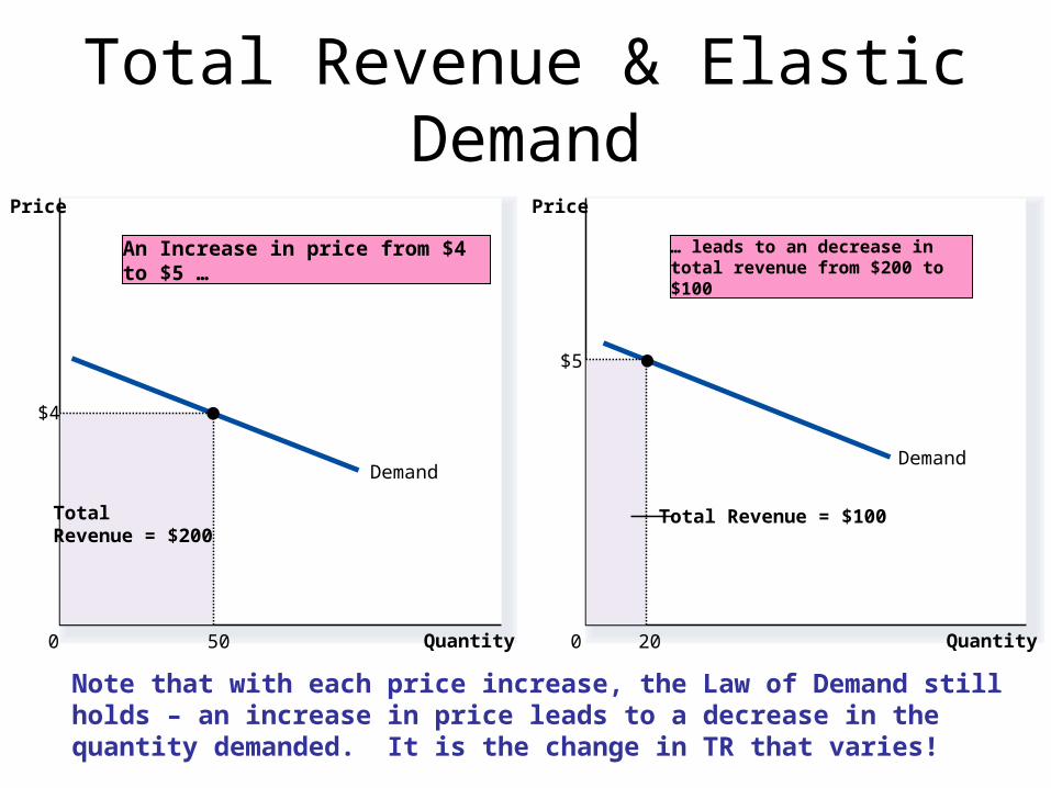
Total Revenue & Elastic Demand
Demand
Quantity0
Price
TotalRevenue = $200
$4
50
Demand
Quantity0
Price
Total Revenue = $100
$5
20
An Increase in price from $4 to $5 … … leads to an decrease in total revenue from $200 to $100
Note that with each price increase, the Law of Demand still holds – an increase in price leads to a decrease in the quantity demanded. It is the change in TR that varies!
D1
D1
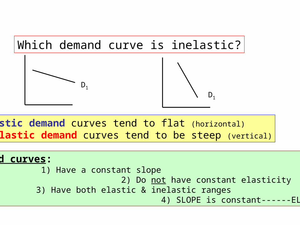
Which demand curve is inelastic?
Elastic demand curves tend to flat (horizontal)
Inelastic demand curves tend to be steep (vertical)
Linear demand curves: 1) Have a constant slope
2) Do not have constant elasticity 3) Have both elastic & inelastic ranges
4) SLOPE is constant------ELASTICITY changes
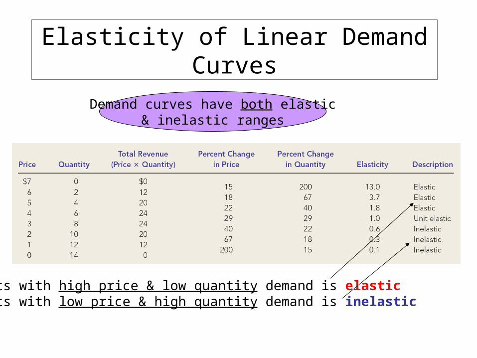
Elasticity of Linear Demand Curves
Demand curves have both elastic& inelastic ranges
Points with high price & low quantity demand is elasticPoints with low price & high quantity demand is inelastic
0 2 64 108 12 14
2
1
4
3
5
6
$7
Elastic Range: Elasticity > 1
Inelastic Range: Elasticity < 1
Price
Quantity
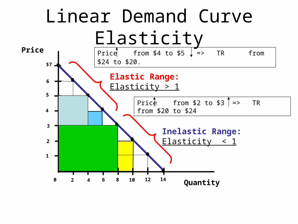
Linear Demand Curve Elasticity
Price from $4 to $5 => TR from $24 to $20.
Price from $2 to $3 => TR from $20 to $24
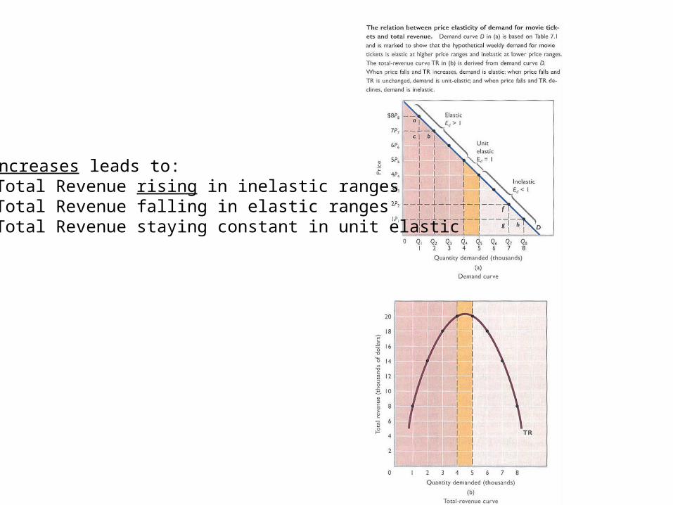
Price increases leads to:Total Revenue rising in inelastic rangesTotal Revenue falling in elastic rangesTotal Revenue staying constant in unit elastic
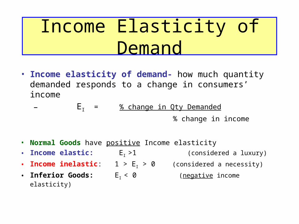
Income Elasticity of Demand
• Income elasticity of demand- how much quantity demanded responds to a change in consumers’ income
– EI = % change in Qty Demanded
% change in income
• Normal Goods have positive Income elasticity
• Income elastic: EI >1 (considered a luxury)
• Income inelastic: 1 > EI > 0 (considered a necessity)
• Inferior Goods: EI < 0 (negative income elasticity)
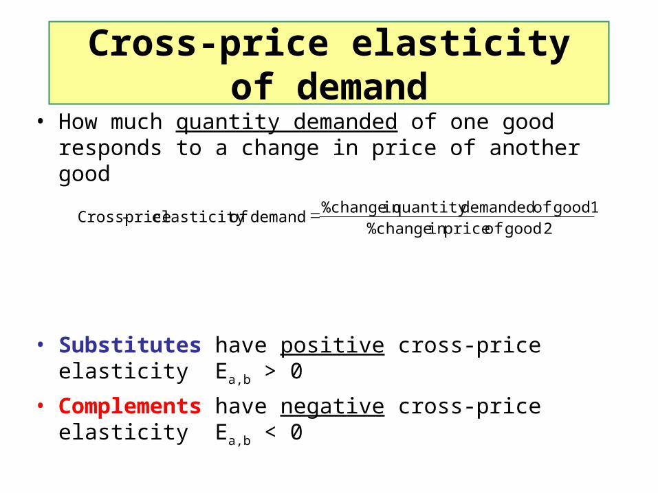
Cross-price elasticity of demand
• How much quantity demanded of one good responds to a change in price of another good
• Substitutes have positive cross-price elasticity Ea,b > 0
• Complements have negative cross-price elasticity Ea,b < 0
2 good of pricein %change1good of demandedquantity in %change
demand of elasticity price-Cross
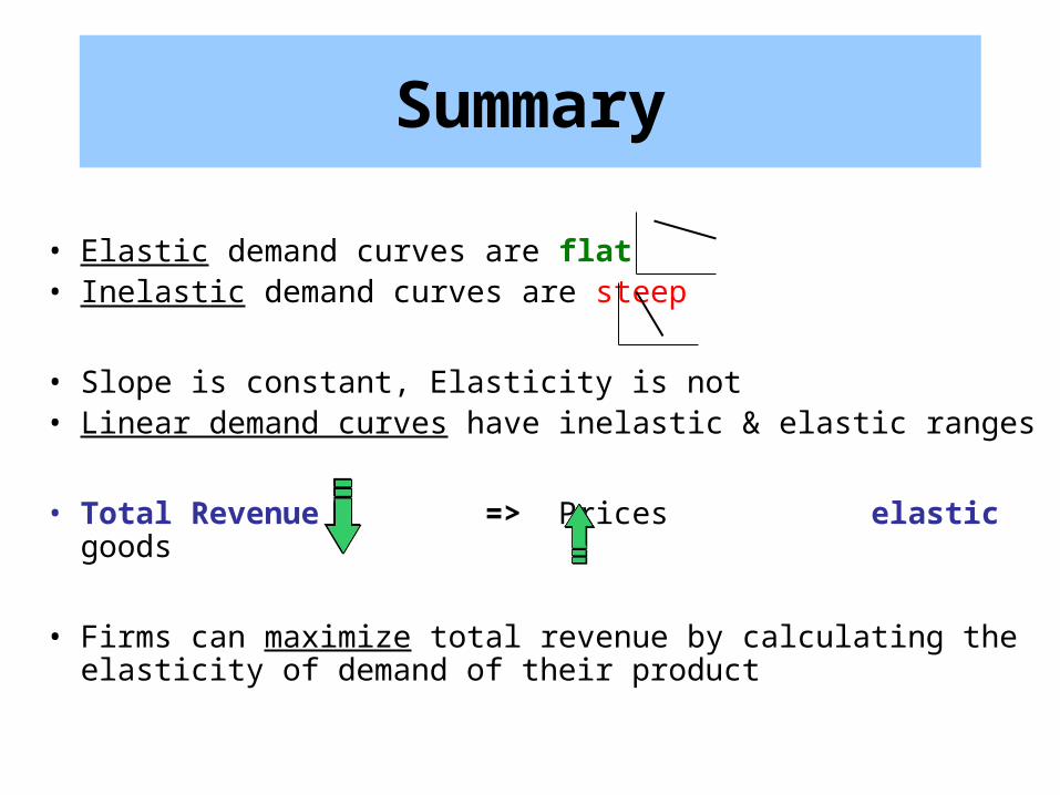
Summary
• Elastic demand curves are flat • Inelastic demand curves are steep
• Slope is constant, Elasticity is not • Linear demand curves have inelastic & elastic ranges
• Total Revenue => Prices elastic goods
• Firms can maximize total revenue by calculating the elasticity of demand of their product
Taxes & Market Equilibrium
Chapter 6
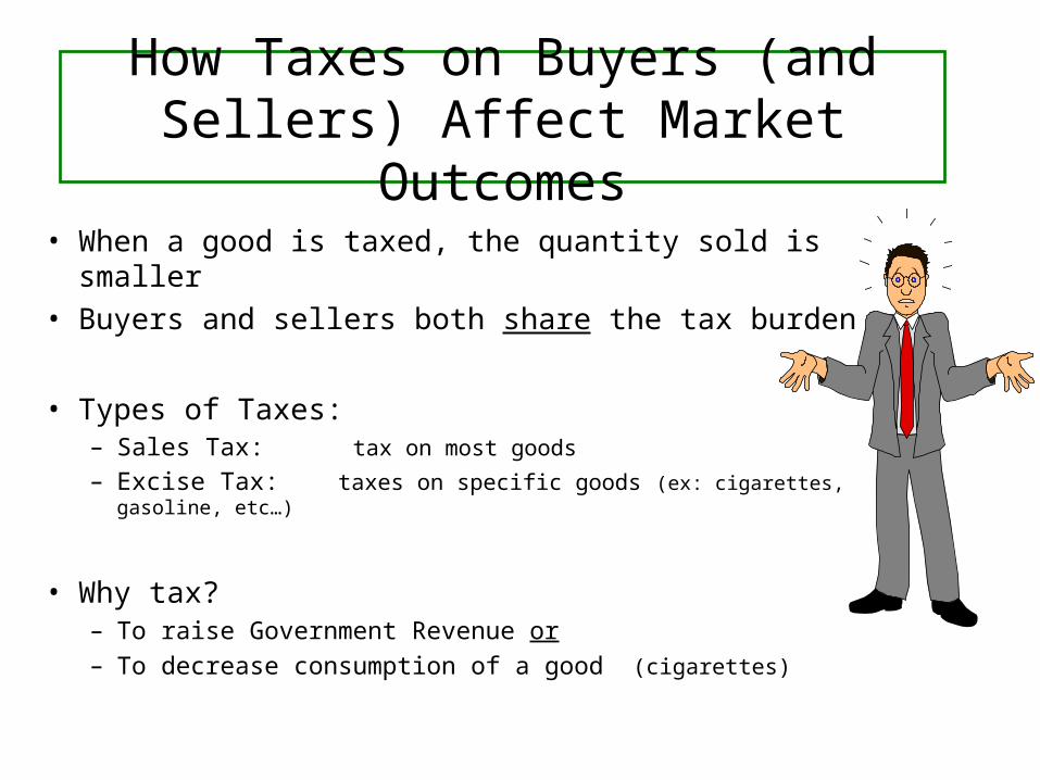
How Taxes on Buyers (and Sellers) Affect Market Outcomes
• When a good is taxed, the quantity sold is smaller • Buyers and sellers both share the tax burden
• Types of Taxes:– Sales Tax: tax on most goods
– Excise Tax: taxes on specific goods (ex: cigarettes, gasoline, etc…)
• Why tax?– To raise Government Revenue or– To decrease consumption of a good (cigarettes)
Elasticity & Tax Incidence
• Tax incidence is the study of who bears the burden of a tax
• Taxes result in a change in market equilibrium
• Buyers pay more & sellers receive less – regardless of whom the tax is levied on
Example: Tax on Buyers• Government places a tax on ice cream of .50 cents
• Does the tax shift the supply or demand curve?
• Supply Curve is not affected – Determinant of supply did not change (TINE & TP)
• Demand Curve will shift left– Price of substitute good in effect fell (remember TIPSEN)
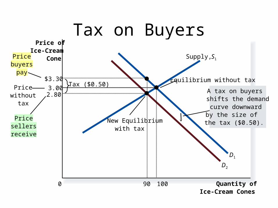
Tax on Buyers
Quantity ofIce-Cream Cones
0
Price ofIce-Cream
Cone
Pricewithout
tax
Pricesellersreceive
Equilibrium without taxTax ($0.50)
Pricebuyers
pay
D1
D2
Supply, S1
A tax on buyersshifts the demandcurve downwardby the size ofthe tax ($0.50).
$3.30
90
New Equilibriumwith tax
2.803.00
100
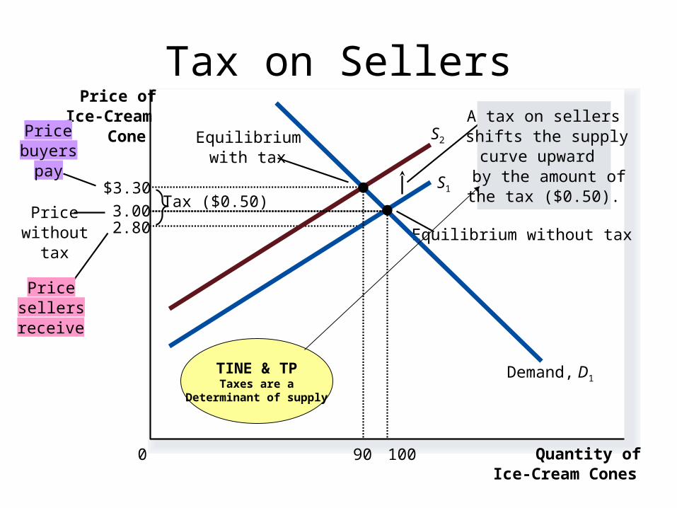
Tax on Sellers
2.80
Quantity ofIce-Cream Cones
0
Price ofIce-Cream
Cone
Pricewithout
tax
Pricesellersreceive
Equilibriumwith tax
Equilibrium without tax
Tax ($0.50)
Pricebuyers
payS1
S2
Demand, D1
A tax on sellersshifts the supplycurve upwardby the amount ofthe tax ($0.50).
3.00
100
$3.30
90
TINE & TPTaxes are a
Determinant of supply
Elasticity and Tax Incidence
• In what proportions is the burden of the tax divided?
• How do the effects of taxes on sellers compare to those levied on buyers?
• It depends on the elasticity of demand & the elasticity of supply.
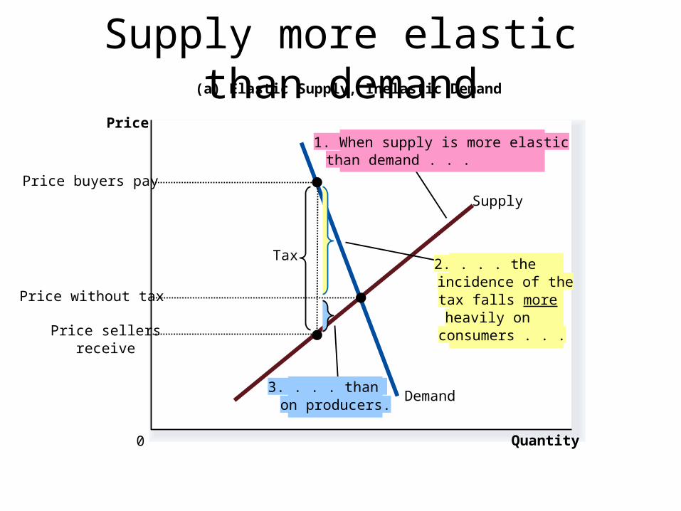
Supply more elastic than demand
Quantity0
Price
Demand
Supply
Tax
Price sellersreceive
Price buyers pay
(a) Elastic Supply, Inelastic Demand
2. . . . theincidence of thetax falls moreheavily onconsumers . . .
1. When supply is more elasticthan demand . . .
Price without tax
3. . . . than on producers.
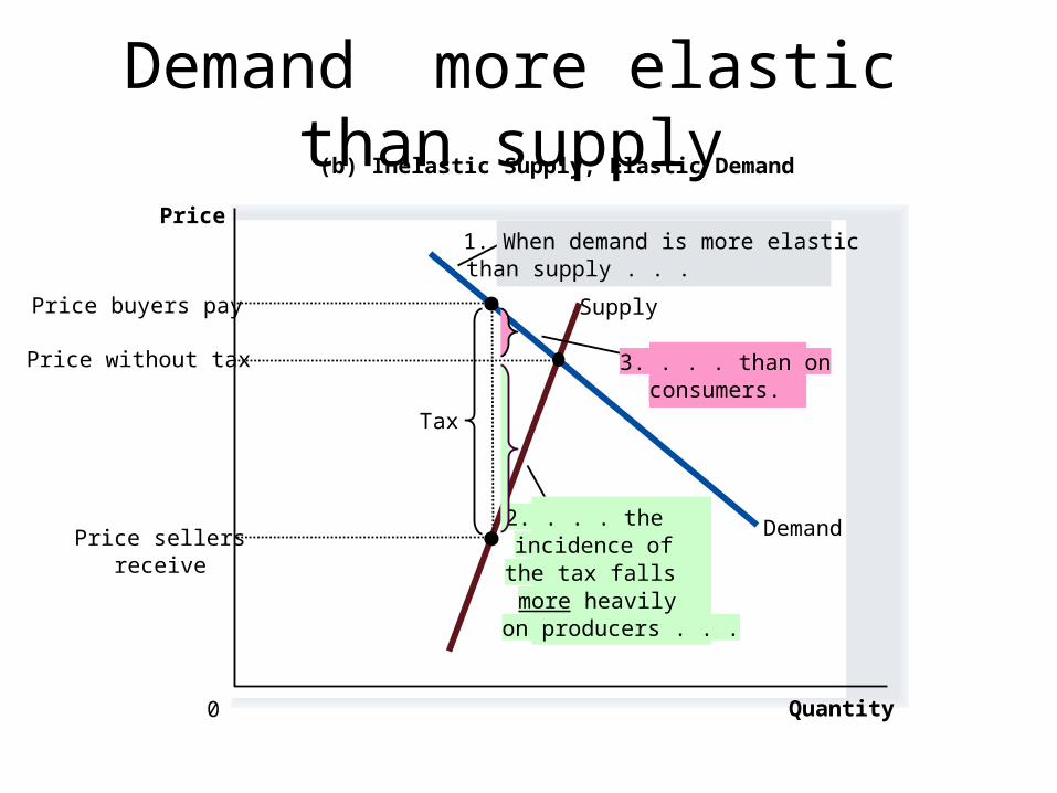
Demand more elastic than supply
Quantity0
Price
Demand
Supply
Tax
Price sellersreceive
Price buyers pay
(b) Inelastic Supply, Elastic Demand
3. . . . than onconsumers.
1. When demand is more elasticthan supply . . .
Price without tax
2. . . . theincidence of the tax falls more heavily on producers . . .
So, how is the burden of the tax divided?
The burden of a tax falls more heavily on the side of the market that is less elastic.
• The incidence of a tax does not depend on whether the tax is levied on buyers or sellers
• It depends on the price elasticities of supply and demand.
• The burden falls on the side of the market that is less elastic
Incidence of Tax Summary
Welfare Economics
Chapter 7: Consumer Surplus
Consumers, Producers & Efficiency of Markets
• Market equilibrium reflects the way markets allocate scarce resources
• Whether the market allocation is desirable can be addressed by welfare economics
• Welfare economics is the study of how the allocation of resources affects economic well-being
Welfare Economics
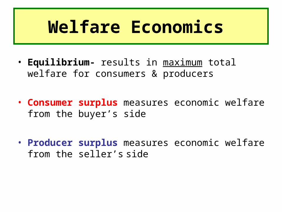
• Equilibrium- results in maximum total welfare for consumers & producers
• Consumer surplus measures economic welfare from the buyer’s side
• Producer surplus measures economic welfare from the seller’s side
CONSUMER SURPLUS
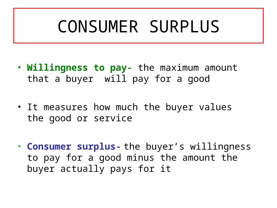
• Willingness to pay- the maximum amount that a buyer will pay for a good
• It measures how much the buyer values the good or service
• Consumer surplus- the buyer’s willingness to pay for a good minus the amount the buyer actually pays for it
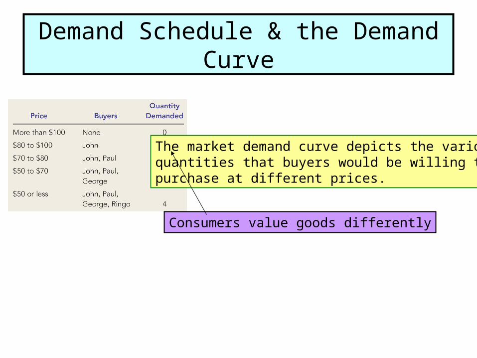
Demand Schedule & the Demand Curve
The market demand curve depicts the various quantities that buyers would be willing to purchase at different prices.
Consumers value goods differently
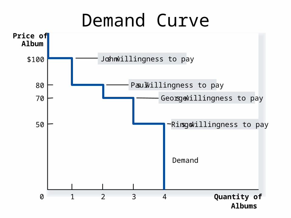
Demand CurvePrice of
Album
0 Quantity ofAlbums
Demand
1 2 3 4
$100 John’s willingness to pay
80 Paul’s willingness to pay
70 George’s willingness to pay
50 Ringo’s willingness to pay
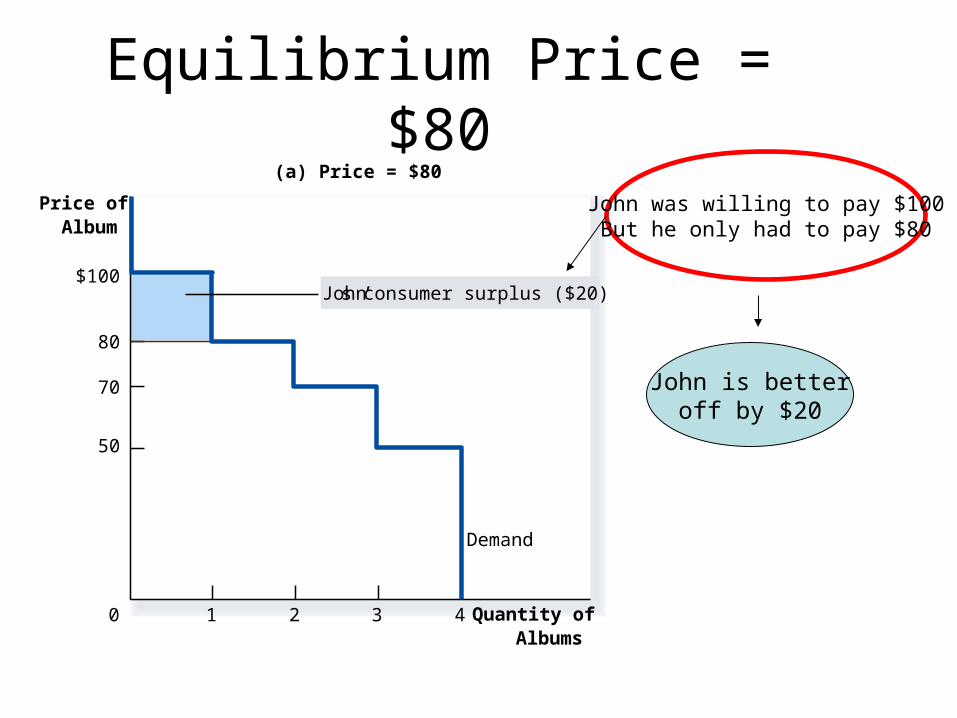
Equilibrium Price = $80(a) Price = $80
Price ofAlbum
50
70
80
0
$100
Demand
1 2 3 4 Quantity ofAlbums
John’s consumer surplus ($20)
John was willing to pay $100But he only had to pay $80
John is betteroff by $20
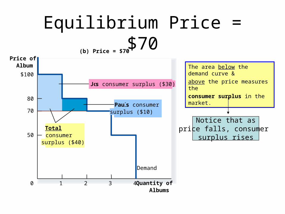
Equilibrium Price = $70(b) Price = $70
Price ofAlbum
50
70
80
0
$100
Demand
1 2 3 4
Totalconsumersurplus ($40)
Quantity ofAlbums
John’s consumer surplus ($30)
Paul’s consumersurplus ($10)
The area below the demand curve &
above the price measures the
consumer surplus in the market.
Notice that asprice falls, consumer
surplus rises
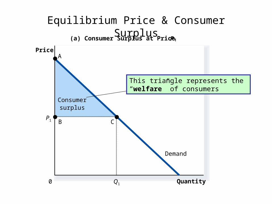
Equilibrium Price & Consumer Surplus
Consumersurplus
Quantity
(a) Consumer Surplus at Price P
Price
0
Demand
P1
Q1
B
A
C
This triangle represents the “welfare” of consumers
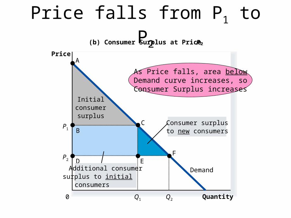
Price falls from P1 to P2
Initialconsumer
surplus
Quantity
(b) Consumer Surplus at Price P
Price
0
Demand
A
BC
D EF
P1
Q1
P2
Q2
Consumer surplusto new consumers
Additional consumersurplus to initial consumers
As Price falls, area belowDemand curve increases, soConsumer Surplus increases
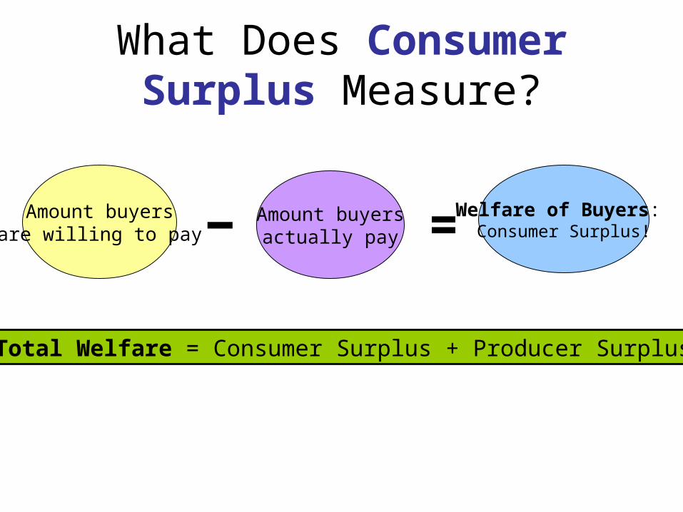
What Does Consumer Surplus Measure?
Amount buyersare willing to pay
Amount buyersactually pay
Welfare of Buyers: Consumer Surplus!- =
Total Welfare = Consumer Surplus + Producer Surplus
Welfare Economics Part II
Chapter 7: Producer Surplus
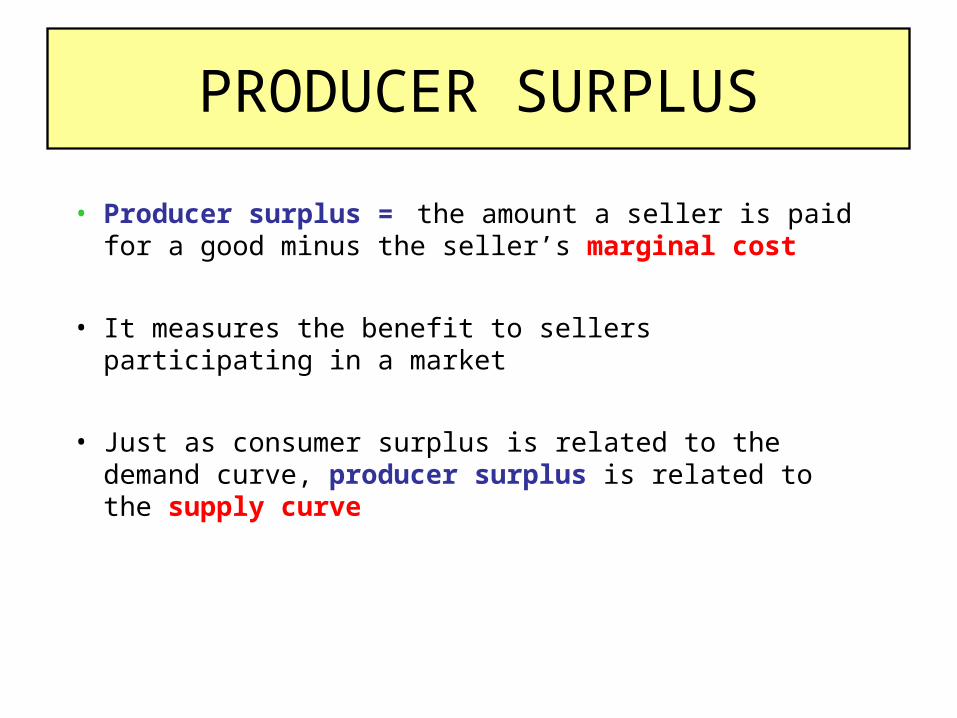
PRODUCER SURPLUS
• Producer surplus = the amount a seller is paid for a good minus the seller’s marginal cost
• It measures the benefit to sellers participating in a market
• Just as consumer surplus is related to the demand curve, producer surplus is related to the supply curve

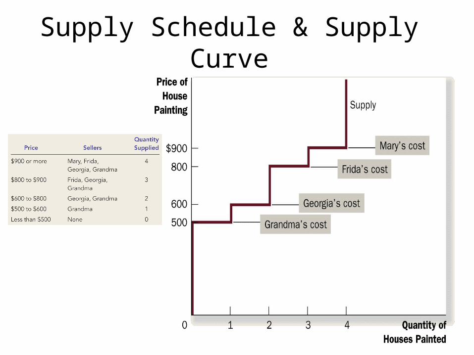
Supply Schedule & Supply Curve
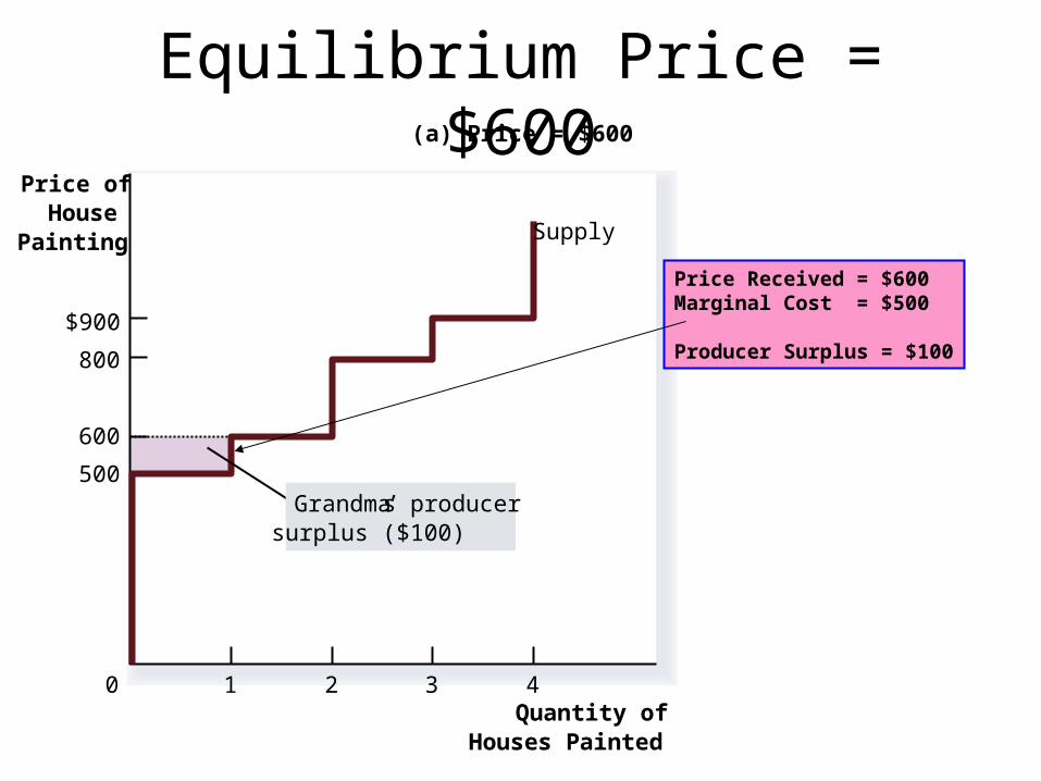
Equilibrium Price = $600
Quantity ofHouses Painted
Price ofHouse
Painting
500
800
$900
0
600
1 2 3 4
(a) Price = $600
Supply
Grandma’s producersurplus ($100)
Price Received = $600Marginal Cost = $500
Producer Surplus = $100

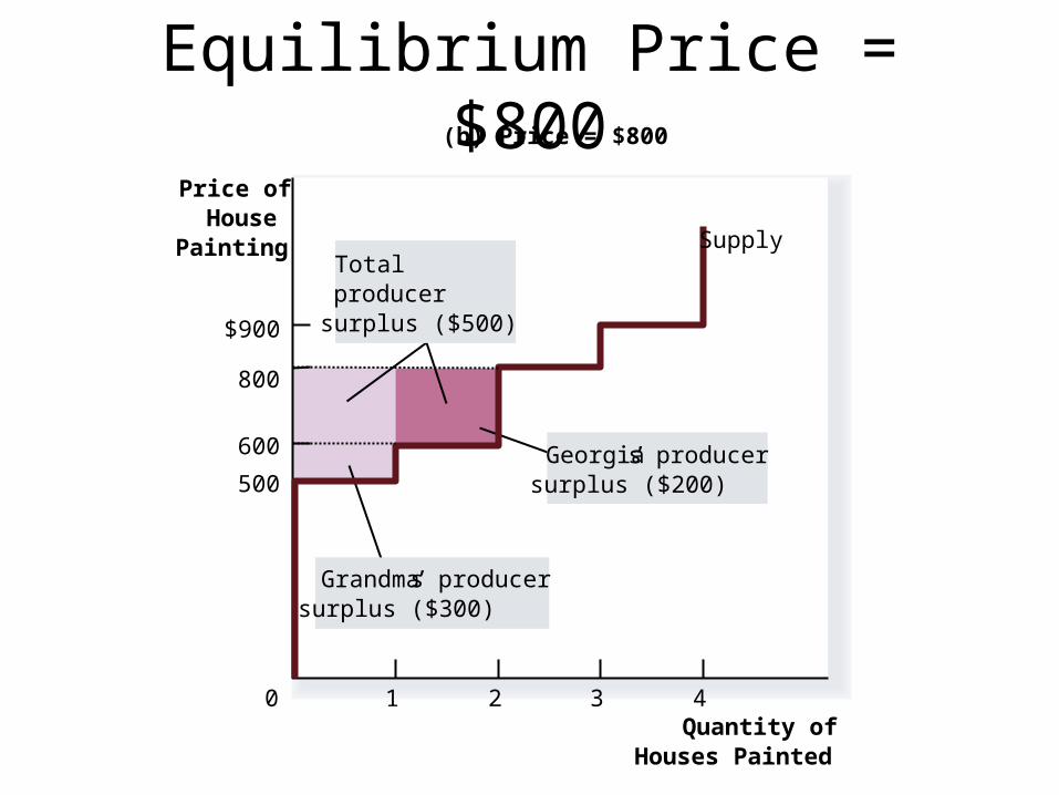
Equilibrium Price = $800
Quantity ofHouses Painted
Price ofHouse
Painting
500
800
$900
0
600
1 2 3 4
(b) Price = $800
Georgia’s producersurplus ($200)
Totalproducersurplus ($500)
Grandma’s producersurplus ($300)
Supply

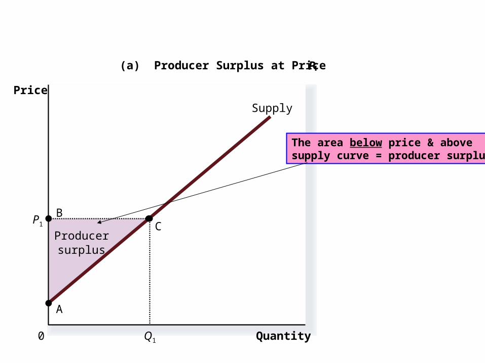
Producersurplus
Quantity
(a) Producer Surplus at Price P
Price
0
Supply
B
A
C
Q1
P1
The area below price & abovesupply curve = producer surplus
Quantity
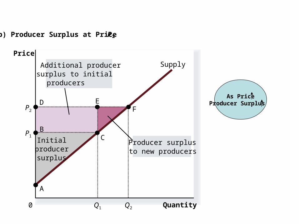
(b) Producer Surplus at Price P
Price
0
P1B
C
Supply
A
Initialproducersurplus
Q1
P2
Q2
Producer surplusto new producers
Additional producersurplus to initialproducers
D EF
As PriceProducer Surplus
EFFICIENCY vs. EQUITY
• Efficiency = resource allocation which maximizes the total surplus received by all members of society
• Equity = the fairness of the distribution of well-being among the various buyers and sellers – Equity is not addressed in free markets
• Free markets naturally (invisible hand) maximize efficiency by maximizing total welfare (consumer surplus + producer surplus)

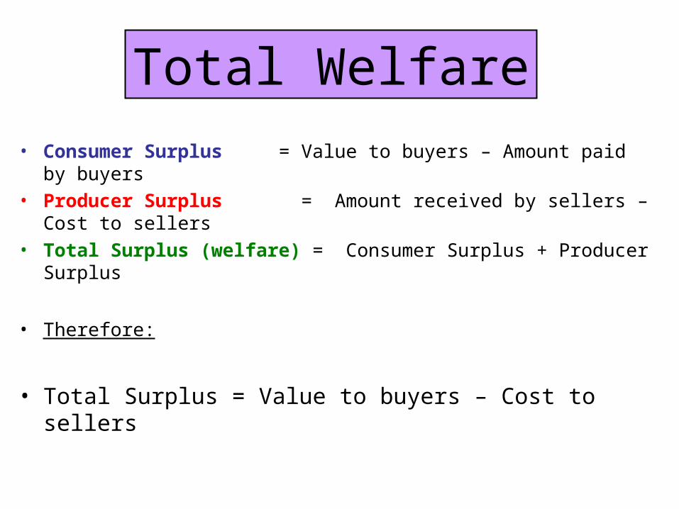
• Consumer Surplus = Value to buyers – Amount paid by buyers• Producer Surplus = Amount received by sellers – Cost to sellers• Total Surplus (welfare) = Consumer Surplus + Producer Surplus
• Therefore:
• Total Surplus = Value to buyers – Cost to sellers
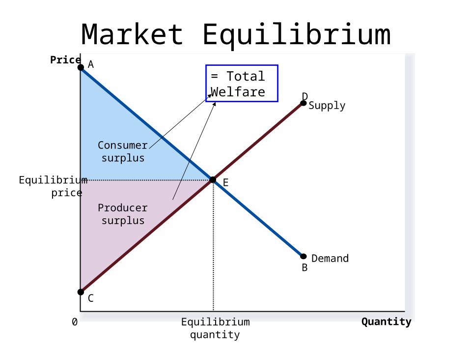
Total Welfare

Market Equilibrium
Producersurplus
Consumersurplus
Price
0 Quantity
Equilibriumprice
Equilibriumquantity
Supply
Demand
A
C
B
D
E
= Total Welfare
Evaluating Free Market Equilibrium
• Free markets allocate the supply of goods to buyers who value them most highly (willingness to pay)
• Free markets allocate the demand for goods to sellers who can produce goods at least cost
• Free markets produce the quantity of goods that maximizes the sum of consumer & producer surplus (Total Welfare/Surplus)

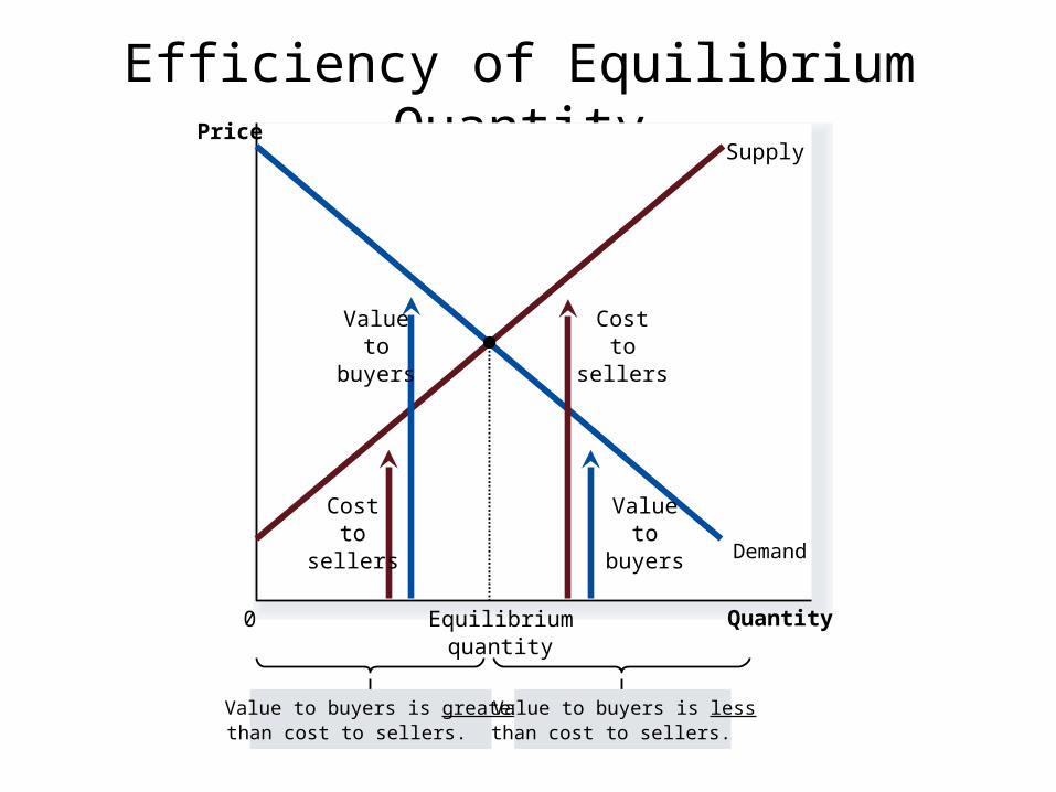
Efficiency of Equilibrium Quantity
Quantity
Price
0
Supply
Demand
Costto
sellers
Costto
sellers
Valueto
buyers
Valueto
buyers
Value to buyers is greaterthan cost to sellers.
Value to buyers is lessthan cost to sellers.
Equilibriumquantity
Worksheet: Lesson 1, Activity 9
• Please complete side 2 of the Consumer/Producer Surplus worksheet

Welfare Economics Part II
Chapter 7: Producer Surplus

PRODUCER SURPLUS
• Producer surplus = the amount a seller is paid for a good minus the seller’s marginal cost
• It measures the benefit to sellers participating in a market
• Just as consumer surplus is related to the demand curve, producer surplus is related to the supply curve
Supply Schedule & Supply Curve

Equilibrium Price = $600
Quantity ofHouses Painted
Price ofHouse
Painting
500
800
$900
0
600
1 2 3 4
(a) Price = $600
Supply
Grandma’s producersurplus ($100)
Price Received = $600Marginal Cost = $500
Producer Surplus = $100
Equilibrium Price = $800
Quantity ofHouses Painted
Price ofHouse
Painting
500
800
$900
0
600
1 2 3 4
(b) Price = $800
Georgia’s producersurplus ($200)
Totalproducersurplus ($500)
Grandma’s producersurplus ($300)
Supply
Producersurplus
Quantity
(a) Producer Surplus at Price P
Price
0
Supply
B
A
C
Q1
P1
The area below price & abovesupply curve = producer surplus

Quantity
(b) Producer Surplus at Price P
Price
0
P1B
C
Supply
A
Initialproducersurplus
Q1
P2
Q2
Producer surplusto new producers
Additional producersurplus to initialproducers
D EF
As PriceProducer Surplus

EFFICIENCY vs. EQUITY
• Efficiency = resource allocation which maximizes the total surplus received by all members of society
• Equity = the fairness of the distribution of well-being among the various buyers and sellers – Equity is not addressed in free markets
• Free markets naturally (invisible hand) maximize efficiency by maximizing total welfare (consumer surplus + producer surplus)
• Consumer Surplus = Value to buyers – Amount paid by buyers• Producer Surplus = Amount received by sellers – Cost to sellers• Total Surplus (welfare) = Consumer Surplus + Producer Surplus
• Therefore:
• Total Surplus = Value to buyers – Cost to sellers
Total Welfare
Market Equilibrium
Producersurplus
Consumersurplus
Price
0 Quantity
Equilibriumprice
Equilibriumquantity
Supply
Demand
A
C
B
D
E
= Total Welfare

Evaluating Free Market Equilibrium
• Free markets allocate the supply of goods to buyers who value them most highly (willingness to pay)
• Free markets allocate the demand for goods to sellers who can produce goods at least cost
• Free markets produce the quantity of goods that maximizes the sum of consumer & producer surplus (Total Welfare/Surplus)
Efficiency of Equilibrium Quantity
Quantity
Price
0
Supply
Demand
Costto
sellers
Costto
sellers
Valueto
buyers
Valueto
buyers
Value to buyers is greaterthan cost to sellers.
Value to buyers is lessthan cost to sellers.
Equilibriumquantity