Embed Size (px)
Citation preview
Do Demand Curves for Currencies SlopeDown? Evidence from the MSCI GlobalIndex Change
Harald HauINSEAD
Massimo MassaINSEAD
Joel PeressINSEAD
Traditional portfolio balance theory derives a downward sloping currency demand func-tion from limited international asset substitutability. Historically, this theory enjoyed littleempirical support. We provide direct evidence by examining the exchange rate effect of amajor redefinition of the MSCI Global Equity Index in 2001 and 2002. The index redefini-tion implied large changes in the representation of different countries in the MSCI GlobalEquity Index and therefore produced strong exogenous equity flows by index funds. Ourevent study reveals that countries with a relatively increasing equity representation experi-enced a relative currency appreciation upon announcement of the index change. Moreover,stock markets that are upweighted (downweighted) feature a higher (lower) permanentcomovement of their currency with the basket of other MSCI currencies. (JEL F21, F31,G11, G15)
To what extent do exogenous demand shocks move financial market prices?Can they propagate from one asset class to another? These are the questionswe address in this article. The first question—commonly referred to as theresilience of a market—has been examined extensively for individual equityprices.1 Much less is known about the resilience of macroeconomic prices suchas exchange rates.2 Yet exchange rates are particularly important and their
Johann-Ruben Schaser provided outstanding research assistance. We also thank Tamas Calderwook from MSCIfor his generous help with the MSCI data. Francis Breedon and Paolo Vitale assisted us with the orderflowdata. Helpful comments were provided by seminar participants at the Western Finance Association Meetings(2005), Saı̈d Business School (Oxford University), Brandeis University, and Humboldt University (Berlin). Sendcorrespondence to Harald Hau, Massimo Massa, and Joel Peress, Department of Finance, Boulevard de Con-stance, 77305 Fontainebleau Cedex, France; telephone: (33)-1-6072-4484, (33)-1-6072-4481, (33)-1-6072-4035;fax: (33)-1-6072-4045. E-mail: [email protected], [email protected], [email protected].
1 We use the term “resilience” here to denote the price impact with respect to uninformative demand shocksas opposed to market depth, which refers to the price impact of general orderflow (from both informed anduninformed investors).
2 It is by no means clear how resilient currencies are. On the one hand, a large literature shows that the demand forstocks slopes down (i.e., their resilience is limited). On the other hand, currencies are viewed as the most liquid
C© The Author 2009. Published by Oxford University Press on behalf of The Society for Financial Studies.All rights reserved. For Permissions, please e-mail: [email protected]:10.1093/rfs/hhp095 Advance Access publication December 3, 2009
alleged misalignment is at the core of a large literature on external imbalances.Imperfect exchange rate resilience underlies the traditional portfolio approachto exchange rates, which derives a downward-sloping demand curve for for-eign balances from imperfect international asset substitutability. The growingquantitative importance of equity flows has increased interest in the portfoliochannel of exchange rate theory.
The second question relates to the propagation of uninformative demandshocks across markets. The traditional literature focuses on frictionless mar-kets in which the propagation is information-based, that is, comovements inasset prices reflect comovements in their fundamental values. However, in thepresence of frictions such as transaction costs, trading restrictions, or imperfectinformation, assets with unrelated fundamentals may comove merely becauseinvestors assign them to similar categories. For example, Barberis and Shleifer(2003) argue that investors tend to categorize assets into styles (e.g., valueversus growth or small-cap versus large-cap), and allocate funds at the level ofthese styles rather than at the individual asset level. As they move funds acrossstyles, they induce a correlation across the returns of assets classified into thesame style, even if the cashflows of these assets are uncorrelated.Barberis,Shleifer, and Wurgler (2005) provide persuasive evidence that such style in-vesting generates comovement among stocks, but there is no evidence to datethat it can induce comovement across different asset classes such as stocks andcurrencies.
The correlation structure between capital flows and exchange rate move-ments has been the subject of much empirical research. But causal inference ishampered by a lack of clear identification. While flows may trigger exchangerate movements, flows may themselves be induced by investors’ trend-chasingbehavior. Similarly, though it can readily be observed that assets belongingto different classes (e.g., equity and fixed income) can move in sync or anti-sync, establishing a directional link from one asset class to another remainsa challenge. This article examines a unique natural experiment in which theeffects of flows on exchange rates can be measured for truly exogenous anduninformative portfolio flows, namely, the rebalancing of the MSCI GlobalEquity Index.
In December 2000, Morgan Stanley Capital International (MSCI) announceda major redefinition of its international equity indices. The new index weightswould be based on the freely floating proportion of a stock’s capitalizationinstead of the market capitalization itself. This implied a large change for theequity representation of many countries in the MSCI Global Equity Index,also referred to as MSCI ACWI (All Country World Index). ApproximatelyUS$300–$350 billion may be directly indexed to MSCI equity indices.3 The
asset class. For example, Menkhoff and Taylor (2007) estimate that currency turnover exceeds equity turnoverby a factor of three in the seven largest financial centers in the world.
3 See the investment newsletter “Spotlight on: Throwing Weights Around,” Hewitt Investment Group, December2000.
2168
The Review of Financial Studies / v 23 n 4 2010
Do Demand Curves for Currencies Slope Down?
up- or downweighting of a country or currency area therefore triggered con-siderable exogenous capital in- or outflow. The MSCI redefinition providesa natural experiment for the exchange rate effect of equity flows. Moreover,because demand shocks clearly originate in the equity market, it offers theopportunity to test whether they are transmitted to the currency market.
We first establish that upweighted stocks earn large excess returns aroundthe announcement event. For example, a strategy that buys a stock upweightedby one standard deviation and sells a stock downweighted by the same amountyields an average abnormal return of 1.18% over a twelve-day window. Thisreturn opportunity is quantitatively similar for various window sizes and mea-sures of stock returns, namely, raw or abnormal relative to an internationalasset pricing model, or returns denominated in U.S. dollars or in local cur-rency. These results conform to previous studies of domestic equity indexchanges. They show that the equity impact of index changes carries over tointernational indices (i.e., that the global demand for stocks slopes down).
We then turn our attention to the currency market. We document that theannouncement event caused a systematic exchange rate appreciation for (rel-atively) upweighted countries. Over an eight-trading-day window around theannouncement event, the sixteen most upweighted currencies appreciate rela-tive to the seventeen most downweighted countries on average by more than2%. While the exact magnitude of the effect is sensitive to the size of the eventwindow and the estimation procedure, its qualitative nature and statistical sig-nificance is robust.
Our findings not only provide evidence that the demand for currencies slopesdown, they also demonstrate that shocks to equities can propagate to curren-cies. Moreover, they have important implications for the current debate aboutinternational current account imbalances. If exogenous capital inflows canstrengthen the domestic exchange rate, then such flows may be the source ofcurrency overvaluation and the cause of current account deficits rather thantheir mere consequence. The issue of causality becomes even more importantin light of the increasing quantitative significance of international equity flowsover the last decade. A further implication is that any anticipation of futuresterilized intervention by central banks can have an immediate exchange rateimpact.4
Finally, we explore whether changes to country weights in the MSCI GlobalEquity Index also modify the permanent correlation structure of exchangerates. Individual stocks have been shown to comove more with an index upontheir addition to the index. We find strong evidence that the same is true ofcurrencies when their representation in a global equity index changes. Weshow that upweighted (downweighted) currencies tend to comove more (less)with the other currencies in the MSCI Global Equity Index.
4 An example of such an annoucement is the Plaza Accord in September 1985 when the G5 countries promised tointervene in currency markets to obtain a devalued U.S. dollar.
1683
The article is structured as follows. In the next section, we discuss the testablehypotheses. In Section 2, we review the literature. Section 3 describes theinstitutional background and provides summary statistics on our experiment.In Section 4, we explain the statistical methodology. The results are presentedin Section 5.1 for the equity market and in Sections 5.2 and 5.3 for the currencymarket. Though we focus our attention on the announcement of the indexredefinition, we discuss briefly in Section 5.4 how the market reacted whenthe index changes were implemented. Section 6 features a discussion of ourfindings. In Section 6.1, we examine whether the index redefinition had anyimpact on currencies’ comovement. In Section 6.2, we discuss whether theeffect on the level of exchange rates should persist. A conclusion follows.
1. Hypotheses
We develop two testable hypotheses that help structure our empirical analysis.The index redefinition presents a natural experiment in which the equity flowsresult from exogenous rebalancing needs of global index funds. This impliesthat these flows are not related to asymmetric information shocks or otherendogenous shocks. The event study therefore allows us to assess directlywhether exogenous global equity flows have an impact on domestic equityprices and exchange rates. Our analysis proceeds in two steps, starting fromthe equity market (Hypothesis H1) and then moving to the currency market(Hypothesis H2). Under Hypothesis H1, stocks are not perfect substitutes forone another in international equity markets—their global demand slopes down.Hence, upweighted stocks see their demand shift up and their price rise, whiledownweighted stocks see their demand shift down and their price fall.
H1. The global demand for stocks slopes down.
Imperfect equity substitutability implies that stock prices react to a global indexredefinition. Stocks that are upweighted (downweighted) in a global index earnpositive (negative) returns.
The alternative hypothesis is that of complete stock substitutability, whichrules out any price effect. A nonrejection of Hypothesis H1 opens the possibilityfor the index redefinition to generate countrywide demand shocks.5 HypothesisH2 investigates whether such shocks have an impact on exchange rates.
H2. The demand for currencies slopes down.
Imperfect currency substitutability implies that exchange rates react to a globalindex redefinition. Currencies that are upweighted (downweighted) in the indexexperience an exchange rate appreciation (depreciation).
5 Hypothesis H1 does not subsume Hypothesis H2. That is, observing an equity effect but no currency effect ispossible, for example, if some international investors are willing to accomodate the excess demand for upweightedcurrencies.
1684
The Review of Financial Studies / v 23 n 4 2010
Do Demand Curves for Currencies Slope Down?
Under this hypothesis, exogenous shocks to the global demand for stocksaggregate at the country level and generate exogenous shocks to the demandfor currencies. If currencies are not perfect substitutes for one another, then theindex change can have a measurable impact on exchange rates. We emphasizethat Hypothesis H2 does not subsume Hypothesis H1. In other words, observinga currency effect but no equity effect is possible. Indeed, if the global demandfor an upweighted country’s equity shifts up but local investors in that countryare willing to accommodate the excess demand, then there will be no observablechange in the country’s equity prices. Yet, to the extent that funds do not flowout of the country, that is, local investors invest their proceeds in local securitiessuch as nonindex stocks or fixed income assets, there will be an excess demandfor the country’s currency, which in turn can trigger a currency appreciation.The alternative to H2 states that the index redefinition does not affect exchangerates.
2. Literature
2.1 Evidence on price pressureOur work is methodologically related to event studies of the equity price im-pact of (domestic equity) index changes. There is evidence that demand curvesfor stocks slope down. S&P 500 index inclusions (exclusions) increase (de-crease) stock prices (Garry and Goetzmann 1986; Harris and Gurel 1986;Shleifer 1986; Dillon and Johnson 1991; Beneish and Whaley 1996; Lynch andMendenhall 1997). Chen (2006) and Onayev and Zdorovtsov (2008) find sim-ilar effects for redefinitions of Russell indices, which represent smaller stocks,and document in addition changes in stocks’ liquidity. Most similar to our study,Kaul, Mehrotra, and Morck (2000) examine index reweighting for stocks inthe Toronto Stock Exchange 300 index and find that upweighted stocks expe-rience a persistent positive price effect. Greenwood (2005) studies the Nikkei225 reweighting. Taking a portfolio approach, he shows both theoretically andempirically that limits to arbitrage are related to the risk contribution of thedemand shock to the portfolio risk of an arbitrageur. Chakrabarti et al. (2005)study changes to MSCI indices as we do, but they examine equities while ourfocus is on currencies. They find that the rebalancing of twenty-nine MSCIcountry indices carried out quarterly between 1998 and 2001 leads to effectsthat are similar to those reported for the United States.
While the short-term price effect of index inclusions is not controversial,its persistence is debated. Shleifer (1986) argues that when a firm is added tothe S&P 500, its stock price permanently increases by 2.79%. His observationis confirmed by Garry and Goetzmann (1986), who find no reversal of short-term announcement returns, but is contradicted by Harris and Gurel (1986) andLynch and Mendenhall (1997), who report some evidence of reversal. Massa,Tong, and Peyer (2004) help reconcile these results by showing that companies
1685
may offset the initial price effect of the index inclusion by issuing moreshares.
While this literature has focused so far on domestic indices and the impactof their redefinitions on the equity market, we examine a global index. Beyondinvestigating whether domestic equity effects carry over to an internationalenvironment, the MSCI experiment allows us to study potential currency ef-fects. Moreover, because demand shocks clearly originate in the equity market,we can provide direct evidence of their propagation to the currency market.That is, we can test whether shocks in the equity market are transmitted tothe currency market. Our article is the first to provide direct evidence of sucha causal linkage. As the transmission of demand shocks from the equity tothe currency market induces a correlation between stocks and currencies—upweighted (downweighted) countries see both their equity and currency ap-preciate (depreciate)—our article also relates to the large literature on comove-ment. But in contrast to this literature, it displays evidence of comovementacross asset classes rather than within an asset class. For example, Barberis,Shleifer, and Wurgler (2005) show that stocks included in the S&P 500 indexcomove more with each other. Boyer (2004) documents a similar phenomenonwhen stocks switch from an S&P/BARRA Value and Growth index to anotherindex.
Our article also connects to a broader literature that assesses whether demandand supply shocks correlate with individual stock returns. Time series studieson block purchases and sales of stocks as well as of the trades of institutionalinvestors have consistently uncovered evidence of temporary price pressure onindividual securities conditional upon unusual demand or supply (Lakonishok,Shleifer, and Vishny 1991, 1992; Chan and Lakonishok 1993, 1995). In theinternational finance literature, Froot, O’Connell, and Seasholes (1998) haveshown that local stock prices are sensitive to international investor flows, andthat transitory inflows have a positive future impact on returns. Focusing onmutual funds, Warther (1995) and Zheng (1999) have documented that investorsupply and demand effects may aggregate to the level of the stock market itself.Goetzmann and Massa (2002) show that, at daily frequency, inflows into S&P500 index funds have a direct impact on the stocks that are part of the index.Generally, the results in this stream of literature are contingent on implicitor explicit identification assumptions. In contrast to the aforementioned eventstudies, causal inference is problematic.
2.2 Price pressure for exchange rates?Our study is also part of the strand of research that links exchange rate move-ments to currency orderflows—a measure of net buying pressure. Evans andLyons (2002a, 2002c) document a strong contemporaneous correlation betweencurrency returns and orderflows. The reason for this correlation, they argue, isthat orderflows proxy for aggregate information flows. They develop models of
61 68
The Review of Financial Studies / v 23 n 4 2010
Do Demand Curves for Currencies Slope Down?
FX trading in the presence of dispersed information that can explain over 60%of the daily Deutsche mark/U.S. dollar exchange rate movements. In a relatedarticle (Evans and Lyons 2002b), they show that trades following macroeco-nomic news have higher price impact. They estimate that the price impact perU.S. dollar traded is about 10% higher per news announcement in the previ-ous hour. The MSCI Global Equity Index rebalancing that we examine here isunlikely to represent a source of macroeconomic information. It allows us tofocus instead on the price impact of uninformative flows.
Uninformative flows lie at the center of the traditional portfolio approachto exchange rates. It views assets in different currencies as imperfect substi-tutes (Kouri 1983; Branson and Henderson 1985). This implies typically thatthe demand for foreign exchange balances slopes downward. Historically, theportfolio balance theory enjoyed little empirical support.6 Hau and Rey (forth-coming) provide microfoundations to the portfolio balance theory in a dynamicincomplete market framework. They derive a positive correlation between cap-ital flows and exchange rate returns and find empirical support for the modelimplications in recent data. Froot and Ramadorai (2005) use a simple VARframework to document very persistent exchange rate effects related to U.S.institutional in- and outflows. Pavlova and Rigobon (2003) and Hau and Rey(2004) use model-based identification assumptions to assess the role of capitalflows for exchange rate movements. In all these studies, causal inference iscontingent on the validity of the identification assumptions. The MSCI indexredefinition provides a natural experiment in which the currency impact ofportfolio flows can be measured for truly exogenous and uninformative flows.
The resilience of the exchange rate is also at the core of a literature on theeffectiveness of central bank interventions (Edison 1993). Recent studies basedon microeconomic data provide evidence that central bank interventions indeedcreate a price effect. Payne and Vitale (2003) show price pressure effects forinterventions by the Swiss central bank. Dominquez (2003) documents a short-term daily and intraday volatility effect related to central bank intervention.However, these studies on central bank interventions are inherently ambiguousabout the nature of the exchange rate effect. Indeed, besides the traditional“portfolio effect” of the intervention, a “signaling effect” provides an alternativeinterpretation of the data. Central bank interventions may reveal informationabout the bank’s future monetary policy.
3. Institutional Background
3.1 MSCI and its index maintenanceMorgan Stanley Capital International Inc. (MSCI) is a leading provider of eq-uity (international and U.S.), fixed income, and hedge fund indices. The MSCI
6 For a survey of the relevant literature, see Rogoff (1984) and Hodrick (1987).
1687
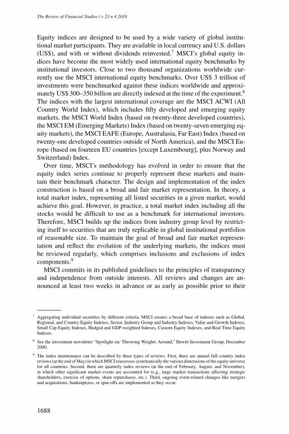
Equity indices are designed to be used by a wide variety of global institu-tional market participants. They are available in local currency and U.S. dollars(US$), and with or without dividends reinvested.7 MSCI’s global equity in-dices have become the most widely used international equity benchmarks byinstitutional investors. Close to two thousand organizations worldwide cur-rently use the MSCI international equity benchmarks. Over US$ 3 trillion ofinvestments were benchmarked against these indices worldwide and approxi-mately US$ 300–350 billion are directly indexed at the time of the experiment.8
The indices with the largest international coverage are the MSCI ACWI (AllCountry World Index), which includes fifty developed and emerging equitymarkets, the MSCI World Index (based on twenty-three developed countries),the MSCI EM (Emerging Markets) Index (based on twenty-seven emerging eq-uity markets), the MSCI EAFE (Europe, Australasia, Far East) Index (based ontwenty-one developed countries outside of North America), and the MSCI Eu-rope (based on fourteen EU countries [except Luxembourg], plus Norway andSwitzerland) Index.
Over time, MSCI’s methodology has evolved in order to ensure that theequity index series continue to properly represent these markets and main-tain their benchmark character. The design and implementation of the indexconstruction is based on a broad and fair market representation. In theory, atotal market index, representing all listed securities in a given market, wouldachieve this goal. However, in practice, a total market index including all thestocks would be difficult to use as a benchmark for international investors.Therefore, MSCI builds up the indices from industry group level by restrict-ing itself to securities that are truly replicable in global institutional portfoliosof reasonable size. To maintain the goal of broad and fair market represen-tation and reflect the evolution of the underlying markets, the indices mustbe reviewed regularly, which comprises inclusions and exclusions of indexcomponents.9
MSCI commits in its published guidelines to the principles of transparencyand independence from outside interests. All reviews and changes are an-nounced at least two weeks in advance or as early as possible prior to their
7 Aggregating individual securities by different criteria, MSCI creates a broad base of indexes such as Global,Regional, and Country Equity Indexes, Sector, Industry Group and Industry Indexes, Value and Growth Indexes,Small Cap Equity Indexes, Hedged and GDP-weighted Indexes, Custom Equity Indexes, and Real Time EquityIndexes.
8 See the investment newsletter “Spotlight on: Throwing Weights Around,” Hewitt Investment Group, December2000.
9 The index maintenance can be described by three types of reviews. First, there are annual full country indexreviews (at the end of May) in which MSCI reassesses systematically the various dimensions of the equity universefor all countries. Second, there are quarterly index reviews (at the end of February, August, and November),in which other significant market events are accounted for (e.g., large market transactions affecting strategicshareholders, exercise of options, share repurchases, etc.). Third, ongoing event-related changes like mergersand acquisitions, bankruptcies, or spin-offs are implemented as they occur.
1688
The Review of Financial Studies / v 23 n 4 2010
Do Demand Curves for Currencies Slope Down?
implementation. Only in rare cases are events announced during market hoursfor implementation on the same or following day.10
3.2 The announcement processIn February 2000, MSCI communicated that it was reviewing its weightingpolicy and that it was considering a move to index weights defined by thefreely floating proportion of the stock value. Such free-float weights wouldtake account of restrictions like Foreign Ownership Limits (FOLs) in differentcountries and therefore would better reflect the limited investibility of manystocks. Free-float weights were subsequently adopted by MSCI’s competitorDow Jones on September 18, 2000. On the next day, MSCI published a con-sultative article on possible changes and elicited comments from its clients. OnDecember 1, 2000, MSCI announced that it would communicate its decisionon the redefinition of the MSCI Global Equity Index on December 10, 2000.Fund managers could by then infer that MSCI’s adoption of free-float weightswas imminent. The second announcement on December 10, 2000, provided thetimetable for the implementation of the index change in two steps and the newtarget for market representation was 85%, up from the previous 60%. To mini-mize the price impact of the redefinition, the equity indices would adjust 50%toward the new index on November 30, 2001, and the remaining adjustmentwas scheduled for May 31, 2002.
MSCI’s decision was broadly in line with the previous consultative article.Only the target level of 85% was somewhat higher (by 5%) and the imple-mentation timetable was somewhat longer than most observers had expected.11
December 10, 2000, therefore marks the confirmation of existing market expec-tations. Most participants appear to have anticipated the adoption of free-floatweights, at least since the first announcement 10 days earlier. An examinationof transaction volumes in the Euro/U.S. dollar spot market confirms this view.We use FX transaction data previously used and documented by Breedon andVitale (2004).12 The data consist of all electronically brokered spot transactionsin both the EBS and Reuters D-2000 trading platforms on any given day fromAugust 1, 2000, to January 24, 2001. The exact size of each transaction (interms of U.S. dollar value) is unknown, but separate volume statistics indi-cate that the average FX spot transaction size in the EBS platform amounts toUS$3.14 million and is somewhat lower for trades in the Reuters system.13 Inthe relevant time period, EBS accounts for approximately 81% of all electron-ically brokered spot trades in the Euro/U.S. dollar market.
10 A more descriptive text announcement is sent out to clients for significant events like additions and deletionsof constituents and changes in free float larger than US$ 5 billion or with an impact of more than 1% of theconstituent’s underlying country index.
11 See again the investment newsletter “Spotlight on: Throwing Weights Around,” Hewitt Investment Group,December 2000.
12 We thank Francis Breedon and Paolo Vitale for generously sharing the data.
13 See Table 3 in Breedon and Vitale (2004).
1689
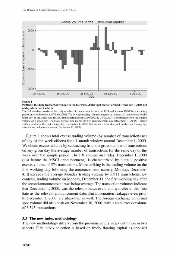
Figure 1Plotted is the daily transaction volume in the Euro/U.S. dollar spot market around December 1, 2000, netof day-of-the-week effectsThe volume data consist of the daily number of transactions in both the EBS and Reuters D-2000 spot tradingplatforms (see Breedon and Vitale 2004). The average trading volume (in terms of number of transactions) for thesame day of the week over the six-month period from 01/08/2000 to 24/01/2001 is subtracted from the tradingvolume on a given day. The black vertical line marks the first announcement day (December 1, 2000). Tradingvolume peaks on the first trading day (December 4, 2000) that follows it but does not on the first trading dayafter the second announcement (December 11, 2000).
Figure 1 shows total excess trading volume (by number of transactions netof day-of-the-week effects) for a 1-month window around December 1, 2000.We obtain excess volume by subtracting from the gross number of transactionson any given day the average number of transactions for the same day of theweek over the sample period. The FX volume on Friday, December 1, 2000(just before the MSCI announcement), is characterized by a small positiveexcess volume of 574 transactions. More striking is the trading volume on thefirst working day following the announcement, namely, Monday, December4. It exceeds the average Monday trading volume by 5,911 transactions. Bycontrast, trading volume on Monday, December 11, the first working day afterthe second announcement, was below average. The transaction volumes indicatethat December 1, 2000, was the relevant news event and we refer to this firstdate as the relevant announcement date. But information leakages even priorto December 1, 2000, are plausible, as well. The foreign exchange abnormalspot volume did also peak on November 30, 2000, with a total excess volumeof 3,545 transactions.
3.3 The new index methodologyThe new methodology differs from the previous equity index definition in twoaspects. First, stock selection is based on freely floating capital as opposed
1690
The Review of Financial Studies / v 23 n 4 2010
Do Demand Curves for Currencies Slope Down?
to market capitalization. Second, the market representation is enhanced in thenew index. MSCI defines the free float of a security as the proportion of sharesoutstanding that is available for purchase by international investors. In prac-tice, limitations on the investment opportunities of international institutionsare common due to so-called “strategic holdings” by either public or privateinvestors. Given that disclosure requirements generally do not permit a clearidentification of “strategic” investments, MSCI labels shareholdings by clas-sifying investors as strategic and nonstrategic. Freely floating shares includethose held by households, investment funds, mutual funds and unit trusts, pen-sion funds, insurance companies, social security funds, and security brokers.The non-free-float shares include those held by governments, companies, banks(excluding trusts), principal officers, board members, and employees. Non-free-float is also defined in terms of foreign ownership restrictions. Such foreignownership limits (FOLs) can come from law, government regulations, companyby-laws, and other authoritative statements. MSCI free float adjusts the marketcapitalization of each security using a factor referred to as the foreign inclusionfactor (FIF). For securities subject to FOLs, the FIF is equal to the lesser ofthe FOL (rounded to the closest 1% increment) and the free float available toforeign investors (rounded up to the closest 5% increment above 15% and tothe closest 1% below a 15% free float). Securities with a FIF of less than 15%across all share classes are generally not eligible for inclusion in the MSCIindices.14
The second goal of the equity index modification was an enhanced marketrepresentation. In its new indices, MSCI targets a free-float-adjusted marketrepresentation of 85% within each industry and country, compared to the 60%share based on market capitalization in the old index. Because of differences inindustry structure, the 85% threshold may not be uniformly achieved. Moreover,the occasional over- and under-representation of industries may also imply thatthe aggregate country representation may deviate from the 85% target.15
The overall index rebalancing effect is illustrated in Figure 2, which plots thepercentage change in index weight for each country in the Global Equity Index(ACWI) as a function of the initial weight. The percentage weight change �wi
is expressed in percentage terms (relative to the mid-point) as
�wi = wni − wo
i12
(wn
i + woi
) ,
where woi and wn
i represent, respectively, the old and new index weight ofcountry i . Normalizing by the average country weight allows us to adjust
14 Exceptions to this general rule are made only in significant cases, where exclusion of a large company wouldcompromise the index’s ability to fully and fairly represent the characteristics of the underlying market.
15 MSCI’s bottom-up approach to index construction may lead to a large company in an industry not being includedin the index, while a smaller company from a different industry might be included.
1691
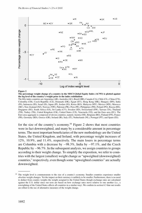
Figure 2The percentage weight change of a country in the MSCI Global Equity Index (ACWI) is plotted againstthe log level of the country’s weight prior to the index redefinitionThe fifty index countries are Argentina (AR), Australia (AU), Brazil (BR), Canada (CA), Chile (CL), China (CN),Colombia (CB), Czech Republic (CZ), Denmark (DK), Egypt (EY), Hong Kong (HK), Hungary (HN), India(IN), Indonesia (ID), Israel (IS), Japan (JP), Jordan (JO), Korea (KO), Malaysia (MY), Mexico (MX), Morocco(MC), New Zealand (NZ), Norway (NW), Pakistan (PK), Peru (PE), Philippines (PH), Poland (PO), Russia (RS),Singapore (SG), South Africa (SA), Sri Lanka (CY), Sweden (SD), Switzerland (SW), Taiwan (TA), Thailand(TH), Turkey (TK), United Kingdom (UK), United States (US), Venezuela (VE), and the Euro area (EU). TheEuro area aggregate is composed of eleven countries, namely Austria (OE), Belgium (BG), Finland (FN), France(FR), Germany (BD), Greece (GR), Ireland (IR), Italy (IT), Netherlands (NL), Portugal (PT), and Spain (ES).
for the size of the country’s economy.16 Figure 2 shows that most countrieswere in fact downweighted, and many by a considerable amount in percentageterms. The most important beneficiaries of the new methodology are the UnitedStates, the United Kingdom, and Ireland, with percentage weight increases of12%, 10.9%, and 11.4%, respectively. The main losers in percentage termsare Columbia with a decrease by −98.3%, India by −97.1%, and the CzechRepublic by −96.7%. In the subsequent analysis, we assign countries to groupsaccording to their weight change. To simplify the exposition, we refer to coun-tries with the largest (smallest) weight change as “upweighted (downweighted)countries,” respectively, even though some “upweighted countries” are actuallydownweighted.
16 The weight level is commensurate to the size of a country’s economy. Smaller countries experience smallerabsolute weight changes. Yet the impact on their currency is unlikely to be smaller. Furthermore, there is no needto deduct from country weights the weight assigned to the United States though exchange rates are calculatedagainst the U.S. dollar since our tests are based on how exchange rates move relative to one another (i.e., areweighting of the United States affects all countries in a similar way). We confirm in section 6.3 that our resultsare robust to the use of alternative measures of the weight change.
1692
The Review of Financial Studies / v 23 n 4 2010
Do Demand Curves for Currencies Slope Down?
The initial sample consists of the fifty countries in the MSCI ACWI.17 Weexclude the United States as the U.S. dollar constitutes our reference currency.We also remove Argentina, Brazil, and Turkey because these countries expe-rienced a major currency crisis before or during the period of our analysis.Since the eleven countries in the Euro zone share one common exchange rate,we aggregate these observations into one so that the old (new) weight equalsthe sum of the eleven country weights in the old (new) index. The final sampleconsists of thirty-six countries with exchange rate data, of which ten are fromdeveloped and twenty-six are from emerging markets. Three countries, namelyChina, Malaysia, and Hong Kong, maintained their currencies pegged to theU.S. dollar. We therefore excluded these three currencies from our sample,which leaves us with thirty-three countries and 2,436 stocks.18 Cross-sectionalsummary statistics for the weight changes of countries and stocks are reportedin Table 1. The table also provides summary statistics on the cross-sectionalexchange rate and stock returns for the announcement event windows. Becauseof the predominant role of the U.S. dollar in the global MSCI index, we expressall exchange rate changes in U.S. dollars per local currency. Generally, wedenote by eit the value of currency i at date t. An appreciation of currency iagainst the U.S. dollar implies �eit > 0. All exchange rate and stock returnsdata were obtained from Datastream. Daily exchange rate returns are based onlog exchange rate changes since the previous (end of the day) London pricefixing.
4. Statistical Methodology
An index fund should rebalance its portfolio close to the implementation of theindex change. This timing will minimize the tracking error relative to the validbenchmark. On the other hand, a possible price impact justifies a more gradualrebalancing toward the new index. Risk arbitrageurs are likely to anticipatethe price impact of index trackers and front-run their reallocation. As in moststudies, we focus our attention on the announcement event (but also discussthe implementation events) and use a symmetric window of a few days aroundit. This is the most appropriate method to capture front-running effects. Weexperiment with both a short window of six trading days and a longer windowof twelve trading days. Generally, we cannot exclude the possibility that a largeproportion of any possible exchange rate effect occurs outside our chosen event
17 The 50 index countries are: Argentina, Australia, Brazil, Canada, Chile, China, Colombia, Czech Republic,Denmark, Egypt, Hong Kong, Hungary, India, Indonesia, Israel, Japan, Jordan, Korea, Malaysia, Mexico,Morocco, New Zealand, Norway, Pakistan, Peru, Philippines, Poland, Russia, Singapore, South Africa, Sri Lanka,Sweden, Switzerland, Taiwan, Thailand, Turkey, United Kingdom, United States, Venezuela, and the 11 Euroarea countries, namely Austria, Belgium, Finland, France, Germany, Greece, Ireland, Italy, Netherlands, Portugal,and Spain.
18 We check that our results are robust to the inclusion of the three countries that experienced a currency crisis orof the three countries with pegged currencies.
1693
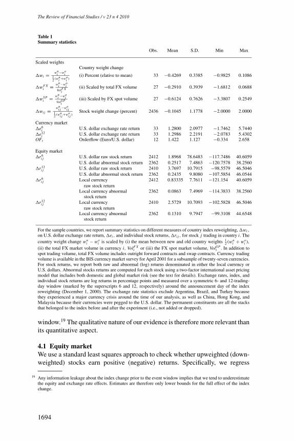
Table 1Summary statistics
Obs. Mean S.D. Min Max
Scaled weightsCountry weight change
�wi = wni −wo
i12 (wn
i +woi )
(i) Percent (elative to mean) 33 −0.4269 0.3385 −0.9825 0.1086
�wF Xi = wn
i −woi
VolF Xi
(ii) Scaled by total FX volume 27 −0.2910 0.3939 −1.6812 0.0688
�wS Pi = wn
i −woi
VolS Pi
(iii) Scaled by FX spot volume 27 −0.6124 0.7626 −3.3807 0.2549
�wi j = wni j −wo
i j12 (wn
i j +woi j )
Stock weight change (percent) 2436 −0.1045 1.1778 −2.0000 2.0000
Currency market�e6
i U.S. dollar exchange rate return 33 1.2800 2.0977 −1.7462 5.7440�e12
i U.S. dollar exchange rate return 33 1.2986 2.2191 −2.0783 5.4302OFt Orderflow (Euro/U.S. dollar) 12 1.422 1.127 −0.334 2.658
Equity market�r6
i j U.S. dollar raw stock return 2412 1.8968 78.6483 −117.7486 40.6059U.S. dollar abnormal stock return 2362 0.2517 7.4863 −120.7578 38.2560
�r12i j U.S. dollar raw stock return 2410 3.7697 10.7915 −98.5579 46.5046
U.S. dollar abnormal stock return 2362 0.2435 9.8080 −107.5854 46.0544�r6
i j Local currency 2412 0.83335 7.7611 −121.154 40.6059raw stock return
Local currency abnormal 2362 0.0863 7.4969 −114.3833 38.2560stock return
�r12i j Local currency 2410 2.5729 10.7093 −102.5828 46.5046
raw stock returnLocal currency abnormal 2362 0.1310 9.7947 −99.3108 44.6548
stock return
For the sample countries, we report summary statistics on different measures of country index reweighting, �wi ,
on U.S. dollar exchange rate return, �ei , and individual stock returns, �ri j , for stock j trading in country i. Thecountry weight change wn
i − woi is scaled by (i) the mean between new and old country weights 1
2 (wni + wo
i ),(ii) the total FX market volume in currency i, VolF X
i or (iii) the FX spot market volume, VolS Pi . In addition to
spot trading volume, total FX volume includes outright forward contracts and swap contracts. Currency tradingvolume is available in the BIS currency market survey for April 2001 for a subsample of twenty-seven currencies.For stock returns, we report both raw and abnormal (log) returns denominated in either the local currency orU.S. dollars. Abnormal stocks returns are computed for each stock using a two-factor international asset pricingmodel that includes both domestic and global market risk (see the text for details). Exchange rates, index, andindividual stock returns are log returns in percentage points and measured over a symmetric 6- and 12-trading-day window (marked by the superscripts 6 and 12, respectively) around the announcement day of the indexreweighting (December 1, 2000). The exchange rate statistics exclude Argentina, Brazil, and Turkey becausethey experienced a major currency crisis around the time of our analysis, as well as China, Hong Kong, andMalaysia because their currencies were pegged to the U.S. dollar. The permanent constituents are all the stacksthat belonged to the index before and after the experiment (i.e., not added or dropped).
window.19 The qualitative nature of our evidence is therefore more relevant thanits quantitative aspect.
4.1 Equity marketWe use a standard least squares approach to check whether upweighted (down-weighted) stocks earn positive (negative) returns. Specifically, we regress
19 Any information leakage about the index change prior to the event window implies that we tend to underestimatethe equity and exchange rate effects. Estimates are therefore only lower bounds for the full effect of the indexchange.
1694
The Review of Financial Studies / v 23 n 4 2010
Do Demand Curves for Currencies Slope Down?
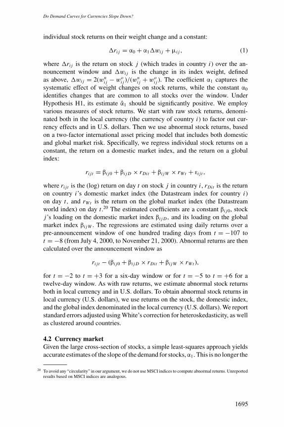
individual stock returns on their weight change and a constant:
�ri j = α0 + α1�wi j + μi j , (1)
where �ri j is the return on stock j (which trades in country i) over the an-nouncement window and �wi j is the change in its index weight, definedas above, �wi j = 2(wn
i j − woi j )/(wn
i j + woi j ). The coefficient α1 captures the
systematic effect of weight changes on stock returns, while the constant α0
identifies changes that are common to all stocks over the window. UnderHypothesis H1, its estimate α̂1 should be significantly positive. We employvarious measures of stock returns. We start with raw stock returns, denomi-nated both in the local currency (the currency of country i) to factor out cur-rency effects and in U.S. dollars. Then we use abnormal stock returns, basedon a two-factor international asset pricing model that includes both domesticand global market risk. Specifically, we regress individual stock returns on aconstant, the return on a domestic market index, and the return on a globalindex:
ri j t = βi j0 + βi j D × rDit + βi jW × rW t + εi j t ,
where ri j t is the (log) return on day t on stock j in country i , rDit is the returnon country i’s domestic market index (the Datastream index for country i)on day t, and rW t is the return on the global market index (the Datastreamworld index) on day t .20 The estimated coefficients are a constant βi j0, stockj’s loading on the domestic market index βi j D, and its loading on the globalmarket index βi jW . The regressions are estimated using daily returns over apre-announcement window of one hundred trading days from t = −107 tot = −8 (from July 4, 2000, to November 21, 2000). Abnormal returns are thencalculated over the announcement window as
ri j t − (βi j0 + βi j D × rDit + βi jW × rW t ),
for t = −2 to t = +3 for a six-day window or for t = −5 to t = +6 for atwelve-day window. As with raw returns, we estimate abnormal stock returnsboth in local currency and in U.S. dollars. To obtain abnormal stock returns inlocal currency (U.S. dollars), we use returns on the stock, the domestic index,and the global index denominated in the local currency (U.S. dollars). We reportstandard errors adjusted using White’s correction for heteroskedasticity, as wellas clustered around countries.
4.2 Currency marketGiven the large cross-section of stocks, a simple least-squares approach yieldsaccurate estimates of the slope of the demand for stocks, α1. This is no longer the
20 To avoid any “circularity” in our argument, we do not use MSCI indices to compute abnormal returns. Unreportedresults based on MSCI indices are analogous.
1695

case when we turn to exchange rates. We therefore assess the relation betweencountry weight changes and currency returns using three different tests. First,we carry out a nonparametric Fisher test. This test examines whether the rankingof the percentage weight change �wi is related to the ranking of the exchangerate change �es
i over the event window, where s denotes the window length.An advantage of the Fisher test is that it represents an exact test and is thereforeparticularly appropriate for small samples. Its null hypothesis is a nonzerocorrelation between the currencies return over the event window and the weightchange. A problem with the test is that such a nonzero correlation might alsoexist outside the event period in normal times. If, for example, exchange ratecorrelations among upweighted exchange rates are systematically differentfrom exchange rate correlations among downweighted currency, then the nullhypothesis of the Fisher test could be rejected over any arbitrary time interval. Inthis case, the Fisher test provides necessary but not sufficient evidence to claimany event-specific effect. Unfortunately, we find evidence of such correlationclustering in the dimension of the country weight changes. Currency pairs ofupweighted countries comove more than currency pairs, consisting of one up-and one downweighted country (we describe the evidence for this phenomenonin the next section). The null hypothesis of the Fisher test may therefore be toogeneral for the problem in hand. We need a model specification that identifies anevent-specific effect against the background of an arbitrary contemporaneouscorrelation structure of all exchange rates.
Our second test addresses the issue of correlation clustering by explicitlyaccounting for the covariance structure of all currencies. To obtain reliablecovariance estimates, we combine the event sample with historical exchangerate data. The historical data cover weekly exchange rate returns from July 1,1996, to July 1, 2000. The weekly returns are measured from the Mondayclosing price to the next Monday closing price. We define a time dummy Dt ,
which equals one for the week with the announcement date (December 1, 2000)and zero for the historical data period. The weekly exchange rate return �eit isregressed on the demeaned scaled weight change �w̄i for currency i (definedas �w̄i = �wi − 1
N
∑Nn=i �wi ) interacted with the time dummy Dt . Formally,
we have
�eit = α0 + α1 Dt + α2(�w̄i × Dt ) + μi t .
We report coefficient estimates α̂1 and α̂2 under both OLS and a panel-error-adjusted procedure. In the latter, the coefficients are estimated using aPrais-Winsten regression and the standard errors are adjusted by assumingthat the disturbances are heteroskedastic and contemporaneously correlatedacross panels and time (which we refer to as a “general covariance struc-ture”). The coefficient α2 captures the systematic effect of the weight changeon the exchange rate, while the coefficient α1 reflects U.S. dollar specific ef-fects common to all currencies. Hypothesis H2 is consistent with a significantlypositive α̂2.
1696
The Review of Financial Studies / v 23 n 4 2010
Do Demand Curves for Currencies Slope Down?
Our third test pushes the analysis of currencies one step further. It accountsfor the possibility that currency trades induced by the index redefinition maynot be spread uniformly over the event window, so identifying the days onwhich they are more intense can improve the power of our tests. It is plausiblethat arbitrageurs take positions simultaneously in all currencies. In that case,above average trading in one currency can serve as a proxy for the “speculativeintensity” common to all currencies.
Euro/U.S. dollar orderflow statistics obtained from Breedon and Vitale(2004) allow us to carry out this analysis. These data consist of the num-ber of daily buy- minus sell-initiated orders in the two important interdealertrading systems EBS and Reuters D-2000 over a window ranging from August2000 to January 2001 (i.e., a period that straddles the announcement). The dailyfrequency of the orderflow data allows us to distinguish trading days character-ized by particularly large U.S. dollar purchases within the event window. TheU.S. equity market was upweighted in the MSCI Global Equity Index relativeto all other markets, including the Euro-denominated equity markets. We ex-pect therefore to observe positive orderflows OFt for days of strong speculativetrading induced by the index rebalancing. For the event window, we define OFt
as the demeaned daily FX orderflow and assume it provides an appropriate in-tertemporal measure of speculative intensity common to all currency markets.We interact orderflow with the demeaned cross-sectional weight change to gen-erate a panel structure with both daily and country variation. This allows us to re-peat the multivariate regression on daily data. We use again a general covariancestructure across all the exchanges and time to control for correlation clustering.The time dummy Dt now equals one for each day around the announcementdate and zero otherwise. In particular, we estimate the linear regression:
�eit = α0 + α1 Dt + α2(�w̄i × Dt ) + α3(OFt × Dt )
+ α4(�w̄i × OFt × Dt ) + μi t .
Under Hypothesis H2, the estimates of α̂2 and/or α̂4 should be significantlypositive. The coefficients α1 and α3 again capture U.S. dollar-specific effectscommon to all currencies.
5. Results
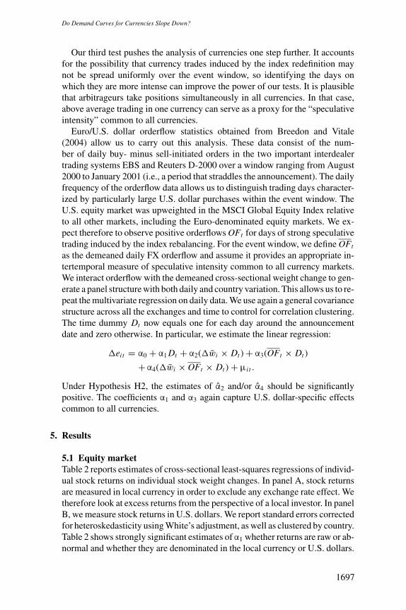
5.1 Equity marketTable 2 reports estimates of cross-sectional least-squares regressions of individ-ual stock returns on individual stock weight changes. In panel A, stock returnsare measured in local currency in order to exclude any exchange rate effect. Wetherefore look at excess returns from the perspective of a local investor. In panelB, we measure stock returns in U.S. dollars. We report standard errors correctedfor heteroskedasticity using White’s adjustment, as well as clustered by country.Table 2 shows strongly significant estimates of α1 whether returns are raw or ab-normal and whether they are denominated in the local currency or U.S. dollars.
1697
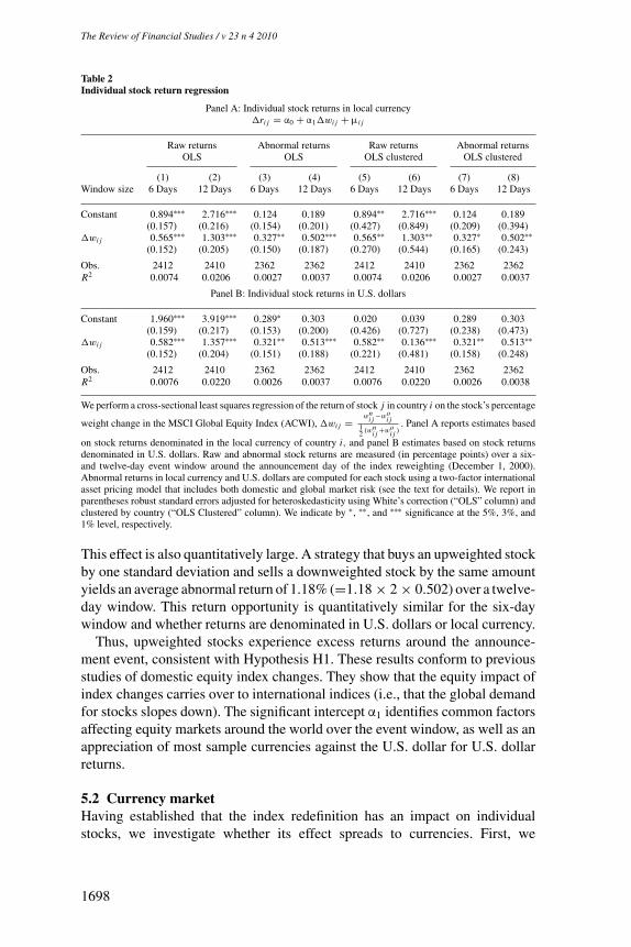
Table 2Individual stock return regression
Panel A: Individual stock returns in local currency�ri j = α0 + α1�wi j + μi j
Raw returns Abnormal returns Raw returns Abnormal returnsOLS OLS OLS clustered OLS clustered
(1) (2) (3) (4) (5) (6) (7) (8)Window size 6 Days 12 Days 6 Days 12 Days 6 Days 12 Days 6 Days 12 Days
Constant 0.894∗∗∗ 2.716∗∗∗ 0.124 0.189 0.894∗∗ 2.716∗∗∗ 0.124 0.189(0.157) (0.216) (0.154) (0.201) (0.427) (0.849) (0.209) (0.394)
�wi j 0.565∗∗∗ 1.303∗∗∗ 0.327∗∗ 0.502∗∗∗ 0.565∗∗ 1.303∗∗ 0.327∗ 0.502∗∗(0.152) (0.205) (0.150) (0.187) (0.270) (0.544) (0.165) (0.243)
Obs. 2412 2410 2362 2362 2412 2410 2362 2362R2 0.0074 0.0206 0.0027 0.0037 0.0074 0.0206 0.0027 0.0037
Panel B: Individual stock returns in U.S. dollars
Constant 1.960∗∗∗ 3.919∗∗∗ 0.289∗ 0.303 0.020 0.039 0.289 0.303(0.159) (0.217) (0.153) (0.200) (0.426) (0.727) (0.238) (0.473)
�wi j 0.582∗∗∗ 1.357∗∗∗ 0.321∗∗ 0.513∗∗∗ 0.582∗∗ 0.136∗∗∗ 0.321∗∗ 0.513∗∗(0.152) (0.204) (0.151) (0.188) (0.221) (0.481) (0.158) (0.248)
Obs. 2412 2410 2362 2362 2412 2410 2362 2362R2 0.0076 0.0220 0.0026 0.0037 0.0076 0.0220 0.0026 0.0038
We perform a cross-sectional least squares regression of the return of stock j in country i on the stock’s percentage
weight change in the MSCI Global Equity Index (ACWI), �wi j = wni j −wo
i j12 (wn
i j +woi j )
. Panel A reports estimates based
on stock returns denominated in the local currency of country i, and panel B estimates based on stock returnsdenominated in U.S. dollars. Raw and abnormal stock returns are measured (in percentage points) over a six-and twelve-day event window around the announcement day of the index reweighting (December 1, 2000).Abnormal returns in local currency and U.S. dollars are computed for each stock using a two-factor internationalasset pricing model that includes both domestic and global market risk (see the text for details). We report inparentheses robust standard errors adjusted for heteroskedasticity using White’s correction (“OLS” column) andclustered by country (“OLS Clustered” column). We indicate by ∗, ∗∗, and ∗∗∗ significance at the 5%, 3%, and1% level, respectively.
This effect is also quantitatively large. A strategy that buys an upweighted stockby one standard deviation and sells a downweighted stock by the same amountyields an average abnormal return of 1.18% (=1.18 × 2 × 0.502) over a twelve-day window. This return opportunity is quantitatively similar for the six-daywindow and whether returns are denominated in U.S. dollars or local currency.
Thus, upweighted stocks experience excess returns around the announce-ment event, consistent with Hypothesis H1. These results conform to previousstudies of domestic equity index changes. They show that the equity impact ofindex changes carries over to international indices (i.e., that the global demandfor stocks slopes down). The significant intercept α1 identifies common factorsaffecting equity markets around the world over the event window, as well as anappreciation of most sample currencies against the U.S. dollar for U.S. dollarreturns.
5.2 Currency marketHaving established that the index redefinition has an impact on individualstocks, we investigate whether its effect spreads to currencies. First, we
1698
The Review of Financial Studies / v 23 n 4 2010
Do Demand Curves for Currencies Slope Down?
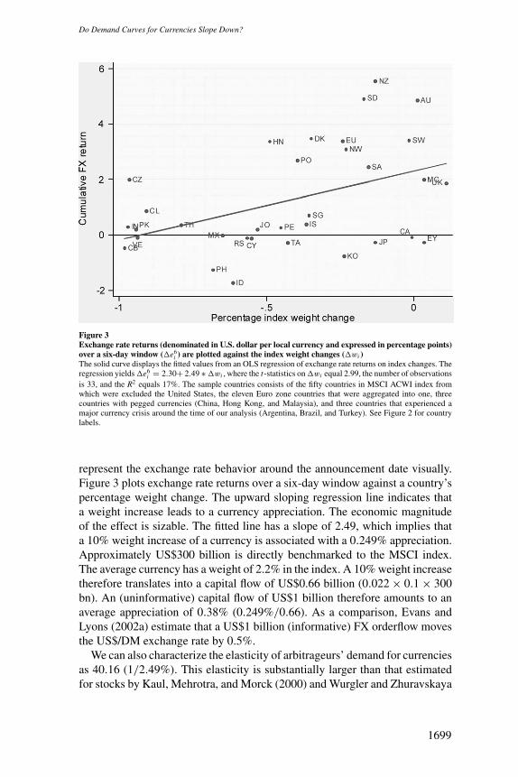
Figure 3Exchange rate returns (denominated in U.S. dollar per local currency and expressed in percentage points)over a six-day window (�e6
i ) are plotted against the index weight changes (�wi )The solid curve displays the fitted values from an OLS regression of exchange rate returns on index changes. Theregression yields �e6
i = 2.30+ 2.49 ∗ �wi , where the t-statistics on �wi equal 2.99, the number of observationsis 33, and the R2 equals 17%. The sample countries consists of the fifty countries in MSCI ACWI index fromwhich were excluded the United States, the eleven Euro zone countries that were aggregated into one, threecountries with pegged currencies (China, Hong Kong, and Malaysia), and three countries that experienced amajor currency crisis around the time of our analysis (Argentina, Brazil, and Turkey). See Figure 2 for countrylabels.
represent the exchange rate behavior around the announcement date visually.Figure 3 plots exchange rate returns over a six-day window against a country’spercentage weight change. The upward sloping regression line indicates thata weight increase leads to a currency appreciation. The economic magnitudeof the effect is sizable. The fitted line has a slope of 2.49, which implies thata 10% weight increase of a currency is associated with a 0.249% appreciation.Approximately US$300 billion is directly benchmarked to the MSCI index.The average currency has a weight of 2.2% in the index. A 10% weight increasetherefore translates into a capital flow of US$0.66 billion (0.022 × 0.1 × 300bn). An (uninformative) capital flow of US$1 billion therefore amounts to anaverage appreciation of 0.38% (0.249%/0.66). As a comparison, Evans andLyons (2002a) estimate that a US$1 billion (informative) FX orderflow movesthe US$/DM exchange rate by 0.5%.
We can also characterize the elasticity of arbitrageurs’ demand for currenciesas 40.16 (1/2.49%). This elasticity is substantially larger than that estimatedfor stocks by Kaul, Mehrotra, and Morck (2000) and Wurgler and Zhuravskaya
1699
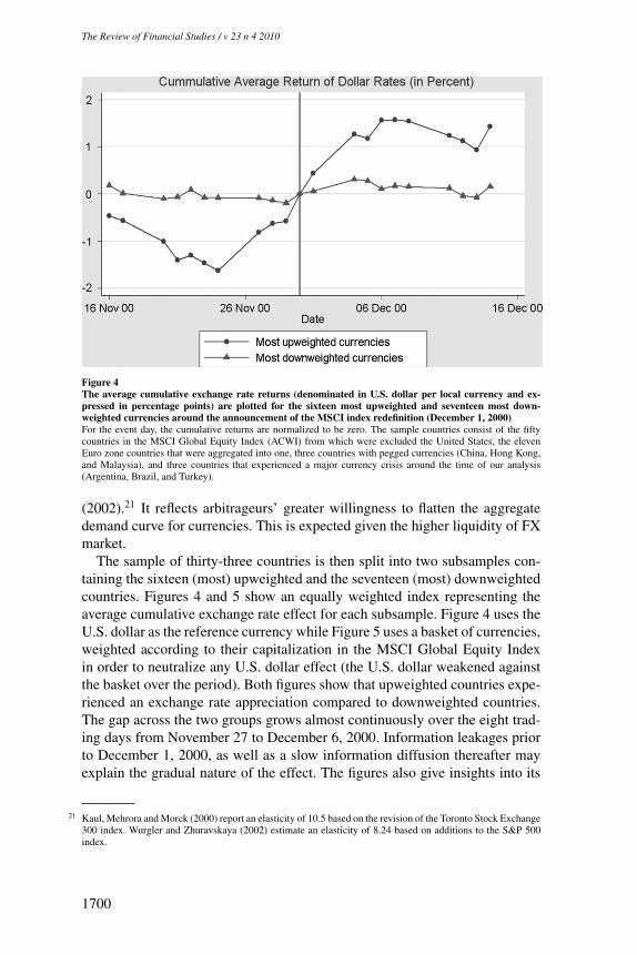
Figure 4The average cumulative exchange rate returns (denominated in U.S. dollar per local currency and ex-pressed in percentage points) are plotted for the sixteen most upweighted and seventeen most down-weighted currencies around the announcement of the MSCI index redefinition (December 1, 2000)For the event day, the cumulative returns are normalized to be zero. The sample countries consist of the fiftycountries in the MSCI Global Equity Index (ACWI) from which were excluded the United States, the elevenEuro zone countries that were aggregated into one, three countries with pegged currencies (China, Hong Kong,and Malaysia), and three countries that experienced a major currency crisis around the time of our analysis(Argentina, Brazil, and Turkey).
(2002).21 It reflects arbitrageurs’ greater willingness to flatten the aggregatedemand curve for currencies. This is expected given the higher liquidity of FXmarket.
The sample of thirty-three countries is then split into two subsamples con-taining the sixteen (most) upweighted and the seventeen (most) downweightedcountries. Figures 4 and 5 show an equally weighted index representing theaverage cumulative exchange rate effect for each subsample. Figure 4 uses theU.S. dollar as the reference currency while Figure 5 uses a basket of currencies,weighted according to their capitalization in the MSCI Global Equity Indexin order to neutralize any U.S. dollar effect (the U.S. dollar weakened againstthe basket over the period). Both figures show that upweighted countries expe-rienced an exchange rate appreciation compared to downweighted countries.The gap across the two groups grows almost continuously over the eight trad-ing days from November 27 to December 6, 2000. Information leakages priorto December 1, 2000, as well as a slow information diffusion thereafter mayexplain the gradual nature of the effect. The figures also give insights into its
21 Kaul, Mehrora and Morck (2000) report an elasticity of 10.5 based on the revision of the Toronto Stock Exchange300 index. Wurgler and Zhuravskaya (2002) estimate an elasticity of 8.24 based on additions to the S&P 500index.
1700
The Review of Financial Studies / v 23 n 4 2010
Do Demand Curves for Currencies Slope Down?
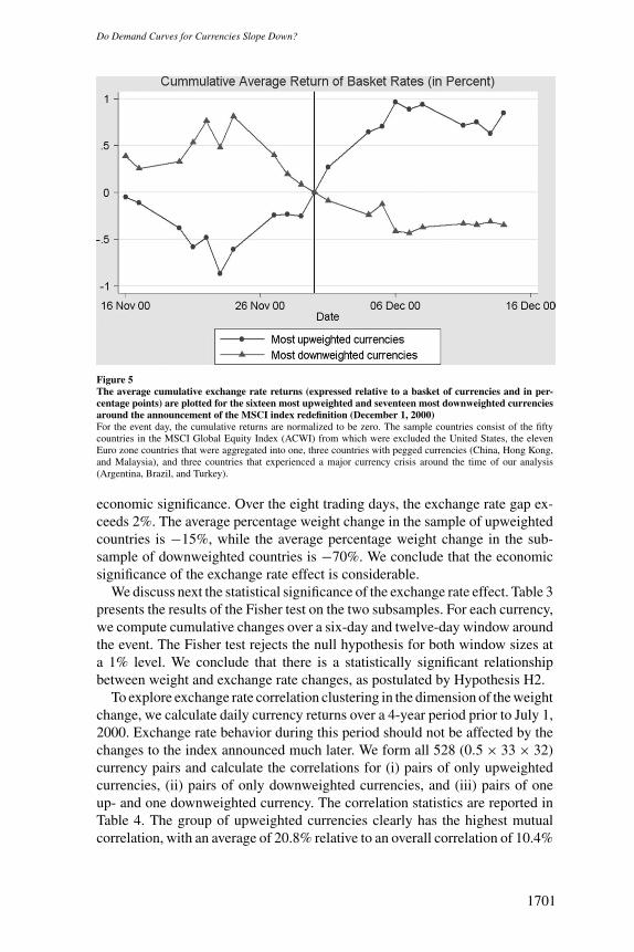
Figure 5The average cumulative exchange rate returns (expressed relative to a basket of currencies and in per-centage points) are plotted for the sixteen most upweighted and seventeen most downweighted currenciesaround the announcement of the MSCI index redefinition (December 1, 2000)For the event day, the cumulative returns are normalized to be zero. The sample countries consist of the fiftycountries in the MSCI Global Equity Index (ACWI) from which were excluded the United States, the elevenEuro zone countries that were aggregated into one, three countries with pegged currencies (China, Hong Kong,and Malaysia), and three countries that experienced a major currency crisis around the time of our analysis(Argentina, Brazil, and Turkey).
economic significance. Over the eight trading days, the exchange rate gap ex-ceeds 2%. The average percentage weight change in the sample of upweightedcountries is −15%, while the average percentage weight change in the sub-sample of downweighted countries is −70%. We conclude that the economicsignificance of the exchange rate effect is considerable.
We discuss next the statistical significance of the exchange rate effect. Table 3presents the results of the Fisher test on the two subsamples. For each currency,we compute cumulative changes over a six-day and twelve-day window aroundthe event. The Fisher test rejects the null hypothesis for both window sizes ata 1% level. We conclude that there is a statistically significant relationshipbetween weight and exchange rate changes, as postulated by Hypothesis H2.
To explore exchange rate correlation clustering in the dimension of the weightchange, we calculate daily currency returns over a 4-year period prior to July 1,2000. Exchange rate behavior during this period should not be affected by thechanges to the index announced much later. We form all 528 (0.5 × 33 × 32)currency pairs and calculate the correlations for (i) pairs of only upweightedcurrencies, (ii) pairs of only downweighted currencies, and (iii) pairs of oneup- and one downweighted currency. The correlation statistics are reported inTable 4. The group of upweighted currencies clearly has the highest mutualcorrelation, with an average of 20.8% relative to an overall correlation of 10.4%
1701
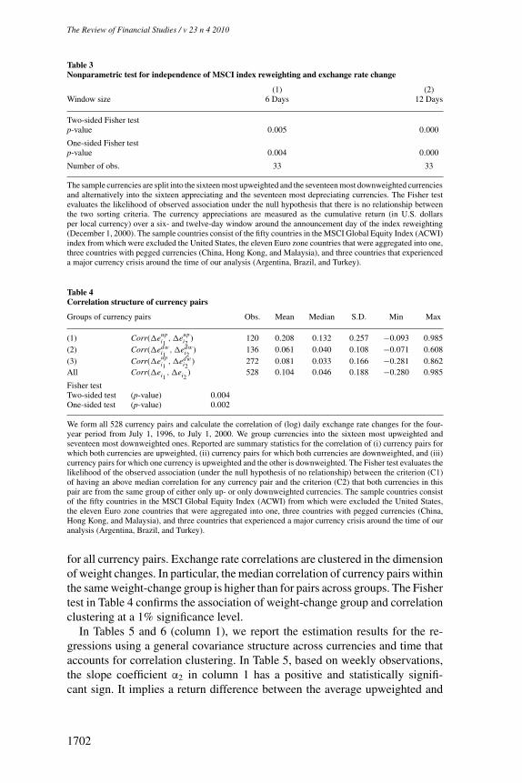
Table 3Nonparametric test for independence of MSCI index reweighting and exchange rate change
(1) (2)Window size 6 Days 12 Days
Two-sided Fisher testp-value 0.005 0.000
One-sided Fisher testp-value 0.004 0.000
Number of obs. 33 33
The sample currencies are split into the sixteen most upweighted and the seventeen most downweighted currenciesand alternatively into the sixteen appreciating and the seventeen most depreciating currencies. The Fisher testevaluates the likelihood of observed association under the null hypothesis that there is no relationship betweenthe two sorting criteria. The currency appreciations are measured as the cumulative return (in U.S. dollarsper local currency) over a six- and twelve-day window around the announcement day of the index reweighting(December 1, 2000). The sample countries consist of the fifty countries in the MSCI Global Equity Index (ACWI)index from which were excluded the United States, the eleven Euro zone countries that were aggregated into one,three countries with pegged currencies (China, Hong Kong, and Malaysia), and three countries that experienceda major currency crisis around the time of our analysis (Argentina, Brazil, and Turkey).
Table 4Correlation structure of currency pairs
Groups of currency pairs Obs. Mean Median S.D. Min Max
(1) Corr(�eupi1
,�eupi2
) 120 0.208 0.132 0.257 −0.093 0.985(2) Corr(�edw
i1, �edw
i2) 136 0.061 0.040 0.108 −0.071 0.608
(3) Corr(�eupi1
,�edwi2
) 272 0.081 0.033 0.166 −0.281 0.862All Corr(�ei1
,�ei2) 528 0.104 0.046 0.188 −0.280 0.985
Fisher testTwo-sided test (p-value) 0.004One-sided test (p-value) 0.002
We form all 528 currency pairs and calculate the correlation of (log) daily exchange rate changes for the four-year period from July 1, 1996, to July 1, 2000. We group currencies into the sixteen most upweighted andseventeen most downweighted ones. Reported are summary statistics for the correlation of (i) currency pairs forwhich both currencies are upweighted, (ii) currency pairs for which both currencies are downweighted, and (iii)currency pairs for which one currency is upweighted and the other is downweighted. The Fisher test evaluates thelikelihood of the observed association (under the null hypothesis of no relationship) between the criterion (C1)of having an above median correlation for any currency pair and the criterion (C2) that both currencies in thispair are from the same group of either only up- or only downweighted currencies. The sample countries consistof the fifty countries in the MSCI Global Equity Index (ACWI) from which were excluded the United States,the eleven Euro zone countries that were aggregated into one, three countries with pegged currencies (China,Hong Kong, and Malaysia), and three countries that experienced a major currency crisis around the time of ouranalysis (Argentina, Brazil, and Turkey).
for all currency pairs. Exchange rate correlations are clustered in the dimensionof weight changes. In particular, the median correlation of currency pairs withinthe same weight-change group is higher than for pairs across groups. The Fishertest in Table 4 confirms the association of weight-change group and correlationclustering at a 1% significance level.
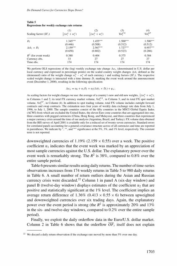
In Tables 5 and 6 (column 1), we report the estimation results for the re-gressions using a general covariance structure across currencies and time thataccounts for correlation clustering. In Table 5, based on weekly observations,the slope coefficient α2 in column 1 has a positive and statistically signifi-cant sign. It implies a return difference between the average upweighted and
2170
The Review of Financial Studies / v 23 n 4 2010
Do Demand Curves for Currencies Slope Down?
Table 5Regressions for weekly exchange rate returns
(1) (2) (3) (4)Scaling factor (SFi ) 1
2 (wni + wo
i ) 12 (wn
i + woi ) VolF X
i VolS Pi
Dt 1.345∗∗∗ 1.455∗∗∗ 1.500∗∗∗ 1.500∗∗∗(0.446) (0.508) (0.512) (0.512)
�w̄i × Dt 2.159∗∗∗ 2.567∗∗∗ 1.727∗∗∗ 0.957∗∗∗(0.658) (0.802) (0.523) (0.286)
R2 (for event week) 0.380 0.404 0.375 0.384Currency obs. 33 27 27 27Time obs. 174 174 174 174
We perform OLS regressions of the (log) weekly exchange rate change �eit (denominated in U.S. dollar perlocal currency and expressed in percentage points) on the scaled country weight changes �w̄i defined as the(demeaned) ratio of the weight change wn
i − woi of each currency i and scaling factors (SFi ). The respective
scaled weight change is interacted with a time dummy Dt marking the event week around the announcementevent (December 1, 2000), resulting in the following specification:
�eit = α0 + α1 Dt + α2(�w̄i × Dt ) + μi t .
As scaling factors for weight changes we use: the average of a country’s new and old new weights, 12 (wn
i + woi ),
in Columns 1 and 2; its total FX currency market volume, VolF Xi , in Column 3; and its total FX spot market
volume, VolS Pi , in Column (4). In addition to spot trading volume, total FX volume includes outright forward
contracts and swap contracts. The estimation uses four years of weekly data exchange rate data from July 1,1996, to July 1, 2000. The sample countries consist of the fifty countries in the MSCI Global Equity Index(ACWI) from which are excluded the United States, the eleven Euro zone countries that are aggregated into one,three countries with pegged currencies (China, Hong Kong, and Malaysia), and three countries that experienceda major currency crisis around the time of our analysis (Argentina, Brazil, and Turkey). FX volume data obtainedfrom the BIS survey of April 2001 is available only for a reduced set of twenty-seven currencies. Standard errorsfor correlated panels accounting for a general covariance structure across of all currencies and time are reportedin parentheses. We indicate by ∗, ∗∗, and ∗∗∗ significance at the 5%, 3%, and 1% level, respectively. The constantterm is not reported.
downweighted currencies of 1.19% (2.159 × 0.55) over a week. The positivecoefficient α1 indicates that the event week was marked by an appreciation ofmost sample currencies against the U.S. dollar. The explanatory power over theevent week is remarkably strong. The R2 is 38%, compared to 0.8% over theentire sample period.
Table 6 presents similar results using daily returns. The number of time-seriesobservations increases from 174 weekly returns in Table 5 to 980 daily returnsin Table 6. A small number of return outliers during the Asian and Russiancurrency crisis were discarded.22 Column 1 in panel A (six-day window) andpanel B (twelve-day window) displays estimates of the coefficient α2 that arepositive and statistically significant at the 1% level. The coefficient implies anaverage return difference of 1.36% (0.413 × 0.55 × 6) between upweightedand downweighted currencies over six trading days. Again, the explanatorypower over the event period is strong (the R2 is approximately 20% and 13%in the six- and twelve-day windows, compared to 0.2% over the entire sampleperiod).
Finally, we exploit the daily orderflow data in the Euro/U.S. dollar market.Column 2 in Table 6 shows that the orderflow OFt itself does not explain
22 We discard a daily return observation if the exchange rate moved by more than 5% over one day.
1703
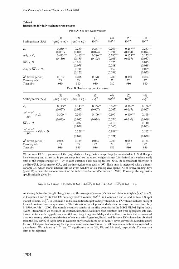
Table 6Regression for daily exchange rate returns
Panel A: Six-day event window
(1) (2) (3) (4) (5) (6)Scaling factor (SFi ) 1
2 (wni + wo
i ) 12 (wn
i + woi ) VolF X
i VolF Xi VolS P
i VolS Pi
Dt 0.230∗∗∗ 0.230∗∗∗ 0.267∗∗∗ 0.267∗∗∗ 0.267∗∗∗ 0.267∗∗∗(0.081) (0.081) (0.094) (0.094) (0.094) (0.094)
�w̄i × Dt 0.413∗∗∗ 0.413∗∗∗ 0.286∗∗∗ 0.286∗∗∗ 0.155∗∗∗ 0.155∗∗∗(0.130) (0.130) (0.105) (0.105) (0.057) (0.057)
OFt × Dt −0.019 0.075 0.075(0.078) (0.088) (0.088)
�w̄i × OFt × Dt 0.191 0.159 0.089(0.123) (0.098) (0.053)
R2 (event period) 0.183 0.206 0.178 0.200 0.180 0.204Currency obs. 33 33 27 27 27 27Time obs. 980 980 980 980 980 980
Panel B: Twelve-day event window
(1) (2) (3) (4) (5) (6)Scaling factor (SFi ) 1
2 (wni + wo
i ) 12 (wn
i + woi ) VolF X
i VolF Xi VolS P
i VolS Pi
Dt 0.143∗∗ 0.143∗∗ 0.166∗∗ 0.166∗∗ 0.166∗∗ 0.166∗∗(0.057) (0.057) (0.067) (0.067) (0.067) (0.067)
wni − wo
i
SFi× Dt 0.300∗∗∗ 0.300∗∗∗ 0.199∗∗∗ 0.199∗∗∗ 0.109∗∗∗ 0.109∗∗∗
(0.093) (0.092) (0.074) (0.074) (0.040) (0.040)OFt × Dt −0.007 0.110 0.110
(0.056) (0.063) (0.063)wn
i − woi
SFi× OFt × Dt 0.229∗∗∗ 0.184∗∗∗ 0.102∗∗∗
(0.088) (0.071) (0.038)
R2 (event period) 0.085 0.129 0.083 0.083 0.083 0.134Currency obs. 33 33 27 27 27 27Time obs. 986 986 986 986 986 986
We perform OLS regressions of the (log) daily exchange rate change �eit (denominated in U.S. dollar perlocal currency and expressed in percentage points) on the scaled weight change �w̄i defined as the (demeaned)ratio of the weight change wn
i − woi of each currency i and scaling factors (SFi ), the (demeaned) orderflow in
the Euro/U.S. dollar market OFt , and the interaction term �w̄i × OFt . Each term is interacted with a dummyvariable Dt , which marks alternatively an event window of six trading days (panel A) or twelve trading days(panel B) around the announcement of the index redefinition (December 1, 2000). Formally, the regressionspecification is given by
�eit = α0 + α1 Dt + α2(�w̄i × Dt ) + α3(OFt × Dt ) + α4(�w̄i × OFt × Dt ) + μi t .
As scaling factors for weight changes we use: the average of a country’s new and old new weights 12 (wn
i + woi ),
in Columns 1 and 2; its total FX currency market volume, VolF Xi , in Columns 3 and 4; and its total FX spot
market volume, VolS Pi , in Columns 5 and 6. In addition to spot trading volume, total FX volume includes outright
forward contracts and swap contracts. The estimation uses 4 years of daily data exchange rate data from July1, 1996, to July 1, 2000. The sample countries consist of the fifty countries in the MSCI Global Equity Index(ACWI) from which we excluded the United States, the eleven Euro zone countries that were aggregated into one,three countries with pegged currencies (China, Hong Kong, and Malaysia), and three countries that experienceda major currency crisis around the time of our analysis (Argentina, Brazil, and Turkey). FX volume data obtainedfrom the BIS survey of April 2001 is available only for a reduced set of twenty-seven currencies. Standard errorsfor correlated panels accounting for a general covariance structure across all currencies and time are reported inparentheses. We indicate by ∗, ∗∗, and ∗∗∗ significance at the 5%, 3%, and 1% level, respectively. The constantterm is not reported.
1704
The Review of Financial Studies / v 23 n 4 2010
Do Demand Curves for Currencies Slope Down?
the intertemporal pattern of exchange rate changes around the announcement.However, the interaction term between weight changes and orderflow duringthe event window days, namely �w̄i × OFt × Dt , produces a statistically sig-nificant positive coefficient in panel B. Intuitively, orderflow in the U.S. dollar/Euro market proxies for the intertemporal intensity of currency speculationin favor of the U.S. dollar. Over the event window, orderflow should pick upcurrency speculation related to the MSCI Global Equity Index weight change.Interacted with the weight change, it proxies for “speculation intensity” in eachindividual currency. The positive sign on the coefficient α4 provides additionalsupport in favor of a downward sloping demand for currencies. The coefficientα2 captures the time average of the weight change impact and remains positive,significant, and of similar magnitude as in column 1.
5.3 Robustness checksIn this section, we check whether the results obtain under alternative normal-izations of the weight change. We relied so far on the change in countries’index representation to predict their currency impact. We used relative weightchange since one would expect this impact to depend on the size of the FXmarkets—currencies in which the daily trading volume is smaller should bemore sensitive to the index redefinition. Specifically, we divided a measure ofthe absolute (U.S. dollar) flow into country i’s currency, wn
i − woi , by the value
(in U.S. dollars) of country i’s equity in the index, (wni + wo
i )/2. We assumedthat the latter is positively related to the size of the market for currency i .
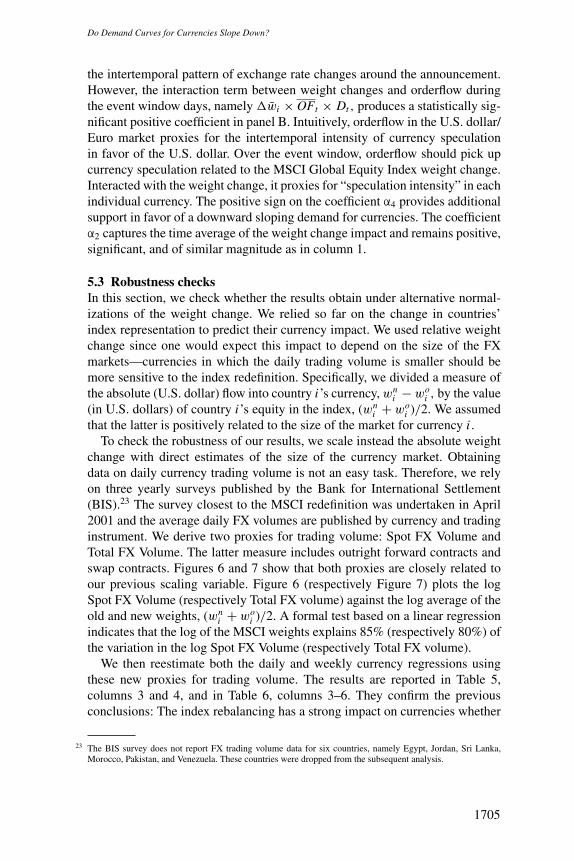
To check the robustness of our results, we scale instead the absolute weightchange with direct estimates of the size of the currency market. Obtainingdata on daily currency trading volume is not an easy task. Therefore, we relyon three yearly surveys published by the Bank for International Settlement(BIS).23 The survey closest to the MSCI redefinition was undertaken in April2001 and the average daily FX volumes are published by currency and tradinginstrument. We derive two proxies for trading volume: Spot FX Volume andTotal FX Volume. The latter measure includes outright forward contracts andswap contracts. Figures 6 and 7 show that both proxies are closely related toour previous scaling variable. Figure 6 (respectively Figure 7) plots the logSpot FX Volume (respectively Total FX volume) against the log average of theold and new weights, (wn
i + woi )/2. A formal test based on a linear regression
indicates that the log of the MSCI weights explains 85% (respectively 80%) ofthe variation in the log Spot FX Volume (respectively Total FX volume).
We then reestimate both the daily and weekly currency regressions usingthese new proxies for trading volume. The results are reported in Table 5,columns 3 and 4, and in Table 6, columns 3–6. They confirm the previousconclusions: The index rebalancing has a strong impact on currencies whether
23 The BIS survey does not report FX trading volume data for six countries, namely Egypt, Jordan, Sri Lanka,Morocco, Pakistan, and Venezuela. These countries were dropped from the subsequent analysis.
1705
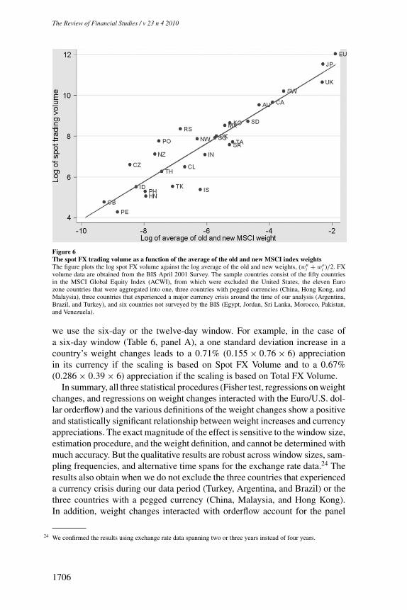
Figure 6The spot FX trading volume as a function of the average of the old and new MSCI index weightsThe figure plots the log spot FX volume against the log average of the old and new weights, (wn
i + woi )/2. FX
volume data are obtained from the BIS April 2001 Survey. The sample countries consist of the fifty countriesin the MSCI Global Equity Index (ACWI), from which were excluded the United States, the eleven Eurozone countries that were aggregated into one, three countries with pegged currencies (China, Hong Kong, andMalaysia), three countries that experienced a major currency crisis around the time of our analysis (Argentina,Brazil, and Turkey), and six countries not surveyed by the BIS (Egypt, Jordan, Sri Lanka, Morocco, Pakistan,and Venezuela).
we use the six-day or the twelve-day window. For example, in the case ofa six-day window (Table 6, panel A), a one standard deviation increase in acountry’s weight changes leads to a 0.71% (0.155 × 0.76 × 6) appreciationin its currency if the scaling is based on Spot FX Volume and to a 0.67%(0.286 × 0.39 × 6) appreciation if the scaling is based on Total FX Volume.
In summary, all three statistical procedures (Fisher test, regressions on weightchanges, and regressions on weight changes interacted with the Euro/U.S. dol-lar orderflow) and the various definitions of the weight changes show a positiveand statistically significant relationship between weight increases and currencyappreciations. The exact magnitude of the effect is sensitive to the window size,estimation procedure, and the weight definition, and cannot be determined withmuch accuracy. But the qualitative results are robust across window sizes, sam-pling frequencies, and alternative time spans for the exchange rate data.24 Theresults also obtain when we do not exclude the three countries that experienceda currency crisis during our data period (Turkey, Argentina, and Brazil) or thethree countries with a pegged currency (China, Malaysia, and Hong Kong).In addition, weight changes interacted with orderflow account for the panel
24 We confirmed the results using exchange rate data spanning two or three years instead of four years.
6701
The Review of Financial Studies / v 23 n 4 2010
Do Demand Curves for Currencies Slope Down?
Figure 7The spot FX trading volume as a function of the average of the old and new MSCI index weightsThe figure plots the log total FX volume against the log average of the old and new weights, (wn
i + woi )/2. In
addition to spot trading volume, Total FX Volume includes outright forward contracts and swap contracts and isobtained from the BIS April 2001 Survey. The sample countries consist of the fifty countries in the MSCI GlobalEquity Index (ACWI) from which were excluded the United States, the eleven Euro zone countries that wereaggregated into one, three countries with pegged currencies (China, Hong Kong, and Malaysia), three countriesthat experienced a major currency crisis around the time of our analysis (Argentina, Brazil, and Turkey), and sixcountries not surveyed by the BIS (Egypt, Jordan, Sri Lanka, Morocco, Pakistan, and Venezuela).
structure of currency returns around the announcement event. This is consis-tent with the idea that orderflow in the Euro/U.S. dollar market proxies forspeculative intensity in all currencies. Overall, the evidence strongly supportsthe notions that shocks originating in the equity market spill over to the currencymarket, and that currencies are imperfect substitutes for one another.
5.4 Implementation effectsWe have focused so far on the market’s reaction to the announcement of theMSCI Global Equity Index redefinition. We examine next the market’s reactionto its implementation. As described above, the redefinition took place in twosteps. On November 31, 2001, half of the changes were implemented for theexisting index constituents and all the new constituents were added at half oftheir final weight. The rest of the changes occurred on May 31, 2002.
Previous studies that distinguish between a price impact occurring at the an-nouncement of an index change from one occurring at its implementation findevidence of a “reversal” on the implementation day. Such a pattern has beenobserved, for example, in the case of changes to the S&P 500 index occurringafter 1990, when S&P started announcing changes to its index. Beneish andWhaley (1996) and Lynch and Mendenhall (1997) report that added stocks
1707
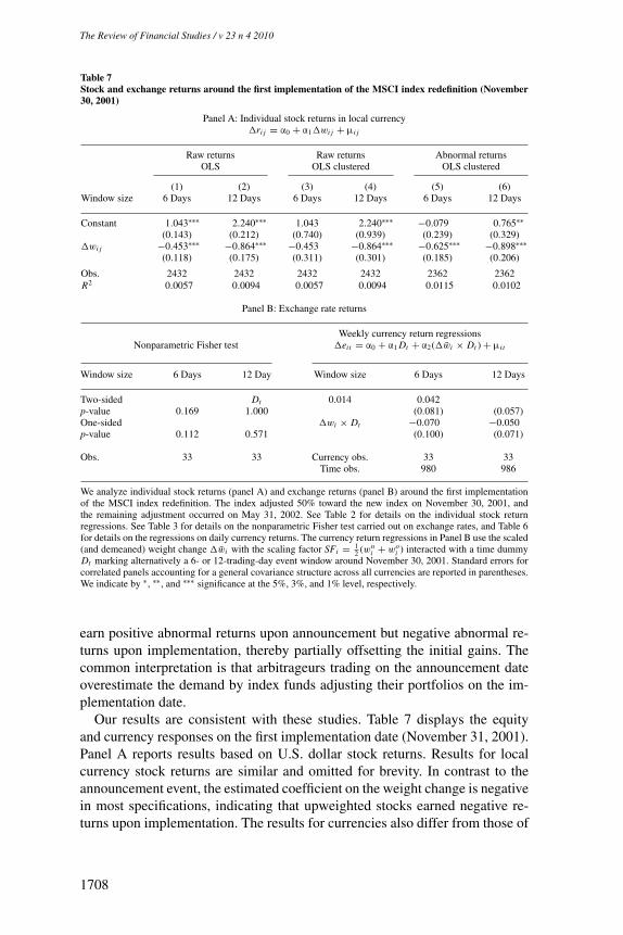
Table 7Stock and exchange returns around the first implementation of the MSCI index redefinition (November30, 2001)
Panel A: Individual stock returns in local currency�ri j = α0 + α1�wi j + μi j
Raw returns Raw returns Abnormal returnsOLS OLS clustered OLS clustered
(1) (2) (3) (4) (5) (6)Window size 6 Days 12 Days 6 Days 12 Days 6 Days 12 Days
Constant 1.043∗∗∗ 2.240∗∗∗ 1.043 2.240∗∗∗ −0.079 0.765∗∗(0.143) (0.212) (0.740) (0.939) (0.239) (0.329)
�wi j −0.453∗∗∗ −0.864∗∗∗ −0.453 −0.864∗∗∗ −0.625∗∗∗ −0.898∗∗∗(0.118) (0.175) (0.311) (0.301) (0.185) (0.206)
Obs. 2432 2432 2432 2432 2362 2362R2 0.0057 0.0094 0.0057 0.0094 0.0115 0.0102
Panel B: Exchange rate returns
Weekly currency return regressionsNonparametric Fisher test �eit = α0 + α1 Dt + α2(�w̄i × Dt ) + μi t
Window size 6 Days 12 Day Window size 6 Days 12 Days
Two-sided Dt 0.014 0.042p-value 0.169 1.000 (0.081) (0.057)One-sided �wi × Dt −0.070 −0.050p-value 0.112 0.571 (0.100) (0.071)
Obs. 33 33 Currency obs. 33 33Time obs. 980 986
We analyze individual stock returns (panel A) and exchange returns (panel B) around the first implementationof the MSCI index redefinition. The index adjusted 50% toward the new index on November 30, 2001, andthe remaining adjustment occurred on May 31, 2002. See Table 2 for details on the individual stock returnregressions. See Table 3 for details on the nonparametric Fisher test carried out on exchange rates, and Table 6for details on the regressions on daily currency returns. The currency return regressions in Panel B use the scaled(and demeaned) weight change �w̄i with the scaling factor SFi = 1
2 (wni + wo
i ) interacted with a time dummyDt marking alternatively a 6- or 12-trading-day event window around November 30, 2001. Standard errors forcorrelated panels accounting for a general covariance structure across all currencies are reported in parentheses.We indicate by ∗, ∗∗, and ∗∗∗ significance at the 5%, 3%, and 1% level, respectively.
earn positive abnormal returns upon announcement but negative abnormal re-turns upon implementation, thereby partially offsetting the initial gains. Thecommon interpretation is that arbitrageurs trading on the announcement dateoverestimate the demand by index funds adjusting their portfolios on the im-plementation date.
Our results are consistent with these studies. Table 7 displays the equityand currency responses on the first implementation date (November 31, 2001).Panel A reports results based on U.S. dollar stock returns. Results for localcurrency stock returns are similar and omitted for brevity. In contrast to theannouncement event, the estimated coefficient on the weight change is negativein most specifications, indicating that upweighted stocks earned negative re-turns upon implementation. The results for currencies also differ from those of
1 087
The Review of Financial Studies / v 23 n 4 2010
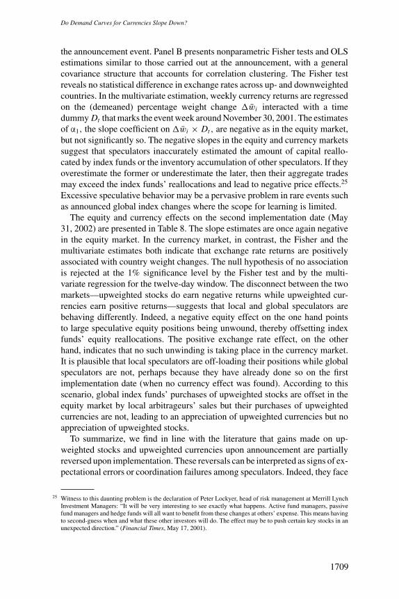
Do Demand Curves for Currencies Slope Down?
the announcement event. Panel B presents nonparametric Fisher tests and OLSestimations similar to those carried out at the announcement, with a generalcovariance structure that accounts for correlation clustering. The Fisher testreveals no statistical difference in exchange rates across up- and downweightedcountries. In the multivariate estimation, weekly currency returns are regressedon the (demeaned) percentage weight change �w̄i interacted with a timedummy Dt that marks the event week around November 30, 2001. The estimatesof α1, the slope coefficient on �w̄i × Dt , are negative as in the equity market,but not significantly so. The negative slopes in the equity and currency marketssuggest that speculators inaccurately estimated the amount of capital reallo-cated by index funds or the inventory accumulation of other speculators. If theyoverestimate the former or underestimate the later, then their aggregate tradesmay exceed the index funds’ reallocations and lead to negative price effects.25
Excessive speculative behavior may be a pervasive problem in rare events suchas announced global index changes where the scope for learning is limited.
The equity and currency effects on the second implementation date (May31, 2002) are presented in Table 8. The slope estimates are once again negativein the equity market. In the currency market, in contrast, the Fisher and themultivariate estimates both indicate that exchange rate returns are positivelyassociated with country weight changes. The null hypothesis of no associationis rejected at the 1% significance level by the Fisher test and by the multi-variate regression for the twelve-day window. The disconnect between the twomarkets—upweighted stocks do earn negative returns while upweighted cur-rencies earn positive returns—suggests that local and global speculators arebehaving differently. Indeed, a negative equity effect on the one hand pointsto large speculative equity positions being unwound, thereby offsetting indexfunds’ equity reallocations. The positive exchange rate effect, on the otherhand, indicates that no such unwinding is taking place in the currency market.It is plausible that local speculators are off-loading their positions while globalspeculators are not, perhaps because they have already done so on the firstimplementation date (when no currency effect was found). According to thisscenario, global index funds’ purchases of upweighted stocks are offset in theequity market by local arbitrageurs’ sales but their purchases of upweightedcurrencies are not, leading to an appreciation of upweighted currencies but noappreciation of upweighted stocks.
To summarize, we find in line with the literature that gains made on up-weighted stocks and upweighted currencies upon announcement are partiallyreversed upon implementation. These reversals can be interpreted as signs of ex-pectational errors or coordination failures among speculators. Indeed, they face
25 Witness to this daunting problem is the declaration of Peter Lockyer, head of risk management at Merrill LynchInvestment Managers: “It will be very interesting to see exactly what happens. Active fund managers, passivefund managers and hedge funds will all want to benefit from these changes at others’ expense. This means havingto second-guess when and what these other investors will do. The effect may be to push certain key stocks in anunexpected direction.” (Financial Times, May 17, 2001).
1709
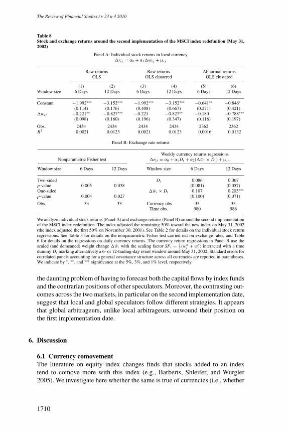
Table 8Stock and exchange returns around the second implementation of the MSCI index redefinition (May 31,2002)
Panel A: Individual stock returns in local currency�ri j = α0 + α1�wi j + μi j
Raw returns Raw returns Abnormal returnsOLS OLS clustered OLS clustered
(1) (2) (3) (4) (5) (6)Window size 6 Days 12 Days 6 Days 12 Days 6 Days 12 Days
Constant −1.992∗∗∗ −3.152∗∗∗ −1.992∗∗∗ −3.152∗∗∗ −0.641∗∗ −0.846∗(0.114) (0.176) (0.408) (0.667) (0.271) (0.421)
�wi j −0.221∗∗ −0.827∗∗∗ −0.221 −0.827∗∗ −0.180 −0.788∗∗∗(0.098) (0.160) (0.196) (0.347) (0.116) (0.197)
Obs. 2434 2434 2434 2434 2362 2362R2 0.0021 0.0123 0.0021 0.0123 0.0016 0.0132
Panel B: Exchange rate returns
Weekly currency returns regressionsNonparametric Fisher test �eit = α0 + α1 Dt + α2(�w̄i × Dt ) + μi t ,
Window size 6 Days 12 Days Window size 6 Days 12 Days
Two-sided Dt 0.086 0.067p-value 0.005 0.038 (0.081) (0.057)One-sided �w̄i × Dt 0.107 0.203∗∗∗p-value 0.004 0.027 (0.100) (0.071)
Obs. 33 33 Currency obs 33 33Time obs. 980 986
We analyze individual stock returns (Panel A) and exchange returns (Panel B) around the second implementationof the MSCI index redefinition. The index adjusted the remaining 50% toward the new index on May 31, 2002(the index adjusted the first 50% on November 30, 2001). See Table 2 for details on the individual stock returnregressions. See Table 3 for details on the nonparametric Fisher test carried out on exchange rates, and Table6 for details on the regressions on daily currency returns. The currency return regressions in Panel B use thescaled (and demeaned) weight change �w̄i with the scaling factor SFi = 1
2 (wni + wo
i ) interacted with a timedummy Dt marking alternatively a 6- or 12-trading-day event window around May 31, 2002. Standard errors forcorrelated panels accounting for a general covariance structure across all currencies are reported in parentheses.We indicate by ∗, ∗∗, and ∗∗∗ significance at the 5%, 3%, and 1% level, respectively.
the daunting problem of having to forecast both the capital flows by index fundsand the contrarian positions of other speculators. Moreover, the contrasting out-comes across the two markets, in particular on the second implementation date,suggest that local and global speculators follow different strategies. It appearsthat global arbitrageurs, unlike local arbitrageurs, unwound their position onthe first implementation date.
6. Discussion
6.1 Currency comovementThe literature on equity index changes finds that stocks added to an indextend to comove more with this index (e.g., Barberis, Shleifer, and Wurgler2005). We investigate here whether the same is true of currencies (i.e., whether
0171
The Review of Financial Studies / v 23 n 4 2010
Do Demand Curves for Currencies Slope Down?
upweighted [downweighted] currencies tend to comove more [less] with theother currencies in the MSCI index).
To test this prediction, we apply the methodology developed by Barberis,Shleifer, and Wurgler (2005). We construct a currency index, representing theaverage return on a basket of currencies. We measure both the equally weightedand the value-weighted return on the basket, where the weights in the latter caseequal the MSCI country weights. We evaluate currencies’ correlation with thebasket by regressing the daily return on a currency i on the daily basket return.A positive slope coefficient reflects the fact that currencies tend to fluctuatetogether. To avoid spurious effects, we remove the contribution of currency i tothe basket. This implies that the basket always consists of all currencies exceptthe U.S. dollar and the currency that is the dependent variable.
We use daily data on exchange rates covering two-year periods before andafter the announcement event (1998–1999 and 2003–2004), and test whethercurrencies’ correlation with the basket has changed. We run the following panelregression:
�eit = α0 + α1Baskett + α2�w̄i + α3 Dt + α4(�w̄i × Baskett )
+ α5(Dt × Baskett ) + α6(Dt × �w̄i )
+ α7(�w̄i × Baskett × Dt ) + εi t , (2)
where �eit measures the percentage change in the currency i on day t , Baskett isthe return on our constructed index on day t (equally or value weighted), �w̄i isthe weight change for currency i , and Dt is a dummy variable that equals 0 in thepre-event period (1998–1999) and 1 in the post-event period (2003–2004). Thecoefficient of interest is α7, which multiplies �w̄i × Baskett × Dt . A positivecoefficient estimate indicates that upweighted currencies comove more withthe basket in the post-event period, as expected. We estimate Equation (2) asa pooled regression with robust standard errors, clustered by both country anddate, as well as a panel regression with errors that are correlated across panels.
The results are reported in Table 9. Panel A uses an equally weighted basket,while panel B uses a value-weighted one. The results show a significantlypositive value for α7, across the different specifications. This suggests thatfollowing the rebalancing, upweighted currencies tend to comove more witheach other than downweighted currencies. The results are not only statisticallysignificant, but also economically large. Indeed, the estimate for α7 is about aslarge as that for α4, the coefficient on the interaction between Baskett and �w̄i .This suggests that the magnitude of the comovement across currencies doublesin the post-event window relative to the pre-event window.
Interestingly, the estimates of α1 and α5 are statistically positive acrossspecifications. The positive coefficient estimate on Baskett , α1, captures thecommonality of shocks across currencies, but it could also reflect shocks to theU.S. dollar, which affect both the currency on the left-hand side and the basket(since currencies are all denominated against the U.S. dollar). This commonality
1711
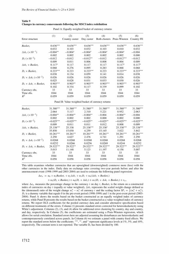
Table 9Changes in currency comovements following the MSCI index redefinition
Panel A: Equally-weighted basket of currency returns
(1) (2) (3) (4) (5) (6)Error structure Country custer Day custer Both clusters Prais-Winsten Country FE
Baskett 0.636∗∗∗ 0.636∗∗∗ 0.636∗∗∗ 0.636∗∗∗ 0.636∗∗∗ 0.636∗∗∗0.032 0.103 0.032 0.103 0.010 0.032
�w̄i (×10−1) −0.004∗∗ −0.004∗ −0.004∗ −0.004∗ −0.004∗ −0.0040.002 0.002 0.002 0.002 0.002 0.000
Dt (×10−2) −0.012 −0.012 −0.012∗∗ −0.012 −0.012∗∗∗ −0.0120.009 0.011 0.006 0.008 0.004 0.009
�w̄i × Baskett 0.117∗ 0.117 0.117 0.117 0.117∗ 0.117∗0.068 0.276 0.095 0.283 0.068 0.068
Dt × Baskett 0.223∗∗∗ 0.223 0.223∗∗∗ 0.223 0.223∗∗∗ 0.223∗∗∗0.038 0.134 0.059 0.141 0.014 0.038
Dt × �w̄i (×10−2) 0.026 0.026 0.026 0.026 0.026 0.0260.025 0.028 0.031 0.033 0.030 0.026
Dt × �w̄i × Baskett 0.903∗∗∗ 0.903∗∗ 0.903∗∗∗ 0.903∗∗∗ 0.903∗∗∗ 0.903∗∗∗0.102 0.334 0.117 0.339 0.099 0.102
Currency obs. 33 33 33 33 33 33Time obs. 1044 1044 1044 1044 1044 1044R2 0.059 0.059 0.059 0.059 0.059 0.059
Panel B: Value-weighted basket of currency returns
Baskett 31.580∗∗∗ 31.580∗∗∗ 31.580∗∗∗ 31.580∗∗∗ 31.580∗∗∗ 31.580∗∗∗2.064 5.117 2.310 5.221 0.952 2.063
�w̄i (×10−1) −0.004∗∗ −0.004∗∗ −0.004∗∗ −0.004 −0.004∗∗ −0.0040.002 0.002 0.002 0.000 0.002 0.000
Dt (×10−2) −0.025∗∗∗ −0.025∗∗∗ −0.025∗∗ −0.025∗∗ −0.025∗∗∗ −0.025∗∗∗0.009 0.011 0.011 0.012 0.008 0.009
�w̄i × Baskett 25.338∗∗∗ 25.338 25.338∗∗∗ 25.338∗ 25.338∗∗∗ 25.338∗∗∗35.850 15.030 4.259 15.145 3.022 3.842
Dt × Baskett 10.261∗∗∗ 10.261∗∗ 10.261∗∗∗ 10.261∗∗ 10.261∗∗∗ 10.261∗∗∗2.250 4.627 2.476 4.741 1.291 2.250
Dt × �w̄i (×10−2) 0.0268 0.0268 0.0268 0.0268 0.0268 0.02680.0252 0.0266 0.0256 0.0269 0.0244 0.0252
Dt × �w̄i × Baskett 29.522∗∗∗ 29.522∗∗ 29.522∗∗∗ 29.522∗∗∗ 29.522∗∗∗ 29.522∗∗∗5.015 11.148 5.123 11.197 4.158 5.007
Currency obs. 33 33 33 33 33 33Time obs. 1044 1044 1044 1044 1044 1044R2 0.058 0.058 0.058 0.058 0.058 0.058
This table examines whether currencies that are upweighted (downweighted) commove more (less) with theother currencies in the index. Daily data on exchange rates covering two-year periods before and after theannouncement event (1998-1999 and 2003-2004) are used to estimate the following panel regression:
�eit = α0 + α1Baskett + α2�w̄i + α3 Dt + α4(�w̄i × Baskett )
+ α5(Dt × Baskett ) + α6(Dt × �w̄i ) + α7(Dt × �w̄i × Baskett ) + εi t ,
where �eit measures the percentage change in the currency i on day t , Baskett is the return on a constructedindex of currencies on day t (equally or value weighted), �w̄i represents the scaled weight change defined asthe (demeaned) ratio of the weight change wn
i − woi of currency i and the scaling factor SFi = 1
2 (wni + wo
i ),Dt is a dummy variable that equals 0 in the pre-event period (1998-1999) and 1 in the post-event period (2003-2004). Panel A shows the results based on the basket constructed as an equally weighed index of currencyreturns, while Panel B presents the results based on the basket constructed as a value-weighted index of currencyreturns. We report OLS coefficients for the pooled currency data and consider alternative specification basedon different treatments of the errors. Column (1) presents standard errors corrected for heteroskedasticity usingWhite’s adjustment. Columns (2), (3), and (4) allow for additional error clustering by country, day and country,and day, respectively. In Column (5), the coefficients are estimated using a Prais-Winsten regression, whichallows for serial correlation. Standard errors here are adjusted assuming the disturbances are heteroskedastic andcontemporaneously correlated across panels. In Column (6) we estimate a panel with country fixed effects. Wereport the standard errors below the coefficients. ∗∗∗, ∗∗, and ∗ represent significance levels at 1%, 5%, and 10%,respectively. The constant term is not reported. The variable Dt has been divided by 100.
2171
The Review of Financial Studies / v 23 n 4 2010
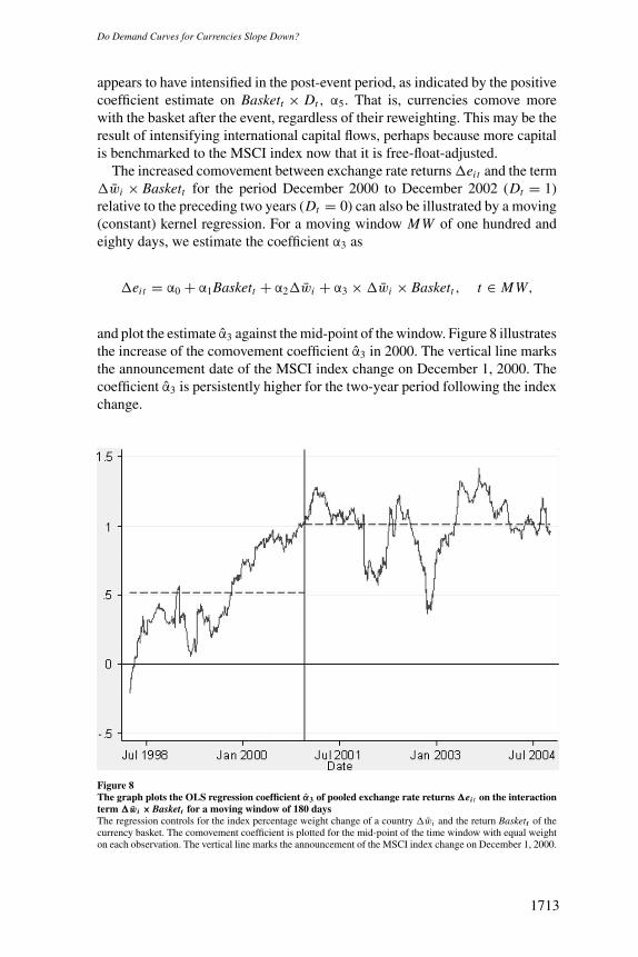
Do Demand Curves for Currencies Slope Down?
appears to have intensified in the post-event period, as indicated by the positivecoefficient estimate on Baskett × Dt , α5. That is, currencies comove morewith the basket after the event, regardless of their reweighting. This may be theresult of intensifying international capital flows, perhaps because more capitalis benchmarked to the MSCI index now that it is free-float-adjusted.
The increased comovement between exchange rate returns �eit and the term�w̄i × Baskett for the period December 2000 to December 2002 (Dt = 1)relative to the preceding two years (Dt = 0) can also be illustrated by a moving(constant) kernel regression. For a moving window MW of one hundred andeighty days, we estimate the coefficient α3 as
�eit = α0 + α1Baskett + α2�w̄i + α3 × �w̄i × Baskett , t ∈ MW,
and plot the estimate α̂3 against the mid-point of the window. Figure 8 illustratesthe increase of the comovement coefficient α̂3 in 2000. The vertical line marksthe announcement date of the MSCI index change on December 1, 2000. Thecoefficient α̂3 is persistently higher for the two-year period following the indexchange.
Figure 8The graph plots the OLS regression coefficient α̂3 of pooled exchange rate returns �ei t on the interactionterm �w̄i × Baskett for a moving window of 180 daysThe regression controls for the index percentage weight change of a country �w̄i and the return Baskett of thecurrency basket. The comovement coefficient is plotted for the mid-point of the time window with equal weighton each observation. The vertical line marks the announcement of the MSCI index change on December 1, 2000.
1713
6.2 Is the currency effect permanent?While our evidence shows that the index redefinition has an effect on the levelof exchange rates that is both statistically and economically sizable in the shortterm, it is unclear whether or not it should persist. This ambiguity is alsopresent in the literature on domestic index additions. While Harris and Gurel(1986) and Schleifer (1986) argue for a permanent effect, Beneish and Whaley(1996), and Lynch and Mendenhall (1997), examining S&P 500 index changesthat were announced before being implemented, find that the announcementeffects are partially reversed on the following days. The literature on blocktrades also reports evidence of temporary price pressure on individual stocksconditional upon unusual demand or supply (Lakonishok, Shleifer, and Vishny1991; Chan and Lakonishok 1993, 1995). In the international finance literature,Froot, O’Connell, and Seasholes (1998) find that local stock prices are sensitiveto international investor flows, and that transitory inflows have a positive futureimpact on returns.
Since our analysis is based on short windows (from six or twelve days aroundeach event for the return analysis, to two years for the comovement analysis),the effect may just be transitory and disappear after a few years. Here, weshare the methodological limitations encountered by the articles that study theequity impact of index changes. Any long-term conclusion requires an esti-mation window so long that the ability of the standard event methodology topin down changes in a statistically meaningful way is hampered. Indeed, otherconfounding effects may alter the relationship, and the underlying assumptionof a constant stock (currency) sensitivity to index weight changes is less accu-rate. However, within the limited two-year window, the results clearly point inthe direction of an increased comovement.
From a theoretical perspective, any discussion of the persistence of theexchange rate effect is still more complicated. According to the standard theoryof money, exchange rates are a function of the relative supply of and demandfor money. Any theoretical conclusion within a monetary framework dependson whether index changes modify the relative money demand temporarilyor permanently. Arguments in favor of both hypotheses can be made. Thereallocation of the index capital itself represents a one-time surge in the relativemoney demand for the upweighted country. But if a higher index representationleads to permanently higher relative asset turnover and generates related cashpositions, changes in the money demand might be of a permanent nature.26
In light of this theoretical ambiguity, we refrain from making any predictionsabout the long-term behavior of exchange rates. But their short-term reaction
26 Moreover, the monetary authorities might respond to any change in the (permanent) relative money demand.If the central bank is concerned about asset price inflation or the price increase of imports, it may reduce themoney supply and this reaction may potentially magnify the short-run exchange rate change. However, under anytype of foreign currency peg, the central bank may respond to the increased money demand by a correspondingincrease in the money supply. The latter channel would neutralize the persistence of the exchange rate effecteven if the money demand does increase permanently. The monetary regime of the country under considerationshould therefore matter for the persistence of the exchange rate effect.
4171
The Review of Financial Studies / v 23 n 4 2010
Do Demand Curves for Currencies Slope Down?
to the index change shown in Figure 4 is still of a striking magnitude and islikely to have real effects.
The evidence of a downward sloping demand curve for currencies presentsevidence for international market segmentation. Assets denominated in differ-ent currencies are imperfect substitutes. Therefore, even uninformative equityflows as those resulting from an index revision result in an exchange rate ad-justment. Such imperfect international asset substitutability is also supportedby evidence on persistent violations of uncovered interest parity, which are theunderlying source of the so-called carry trades. International arbitrage forcesin the currency market appear too weak to maintain uncovered interest rateparty. They also appear too weak to provide a flat currency supply curve toaccommodate uninformative equity flows from an index revision.
7. Conclusions
The exchange rate reaction to exogenous capital flows has long been an openissue in international finance. Empirical work suffered from a lack of clearidentification of capital flow shocks. At the same time, the growing quantitativeimportance of international equity flows has revived interest in the traditionalportfolio channel of exchange rate determination. The MSCI Global EquityIndex redefinition announced in December 2000 provides an ideal naturalexperiment to examine the impact of clearly exogenous equity flows on a largenumber of exchange rates. Moreover, because demand shocks clearly originatein the equity market, the redefinition offers the opportunity to test whether theyare transmitted to the currency market.
We find that upweighted stocks and upweighted currencies earn large excessreturns around the announcement of the index change. In other words, the globaldemand for stocks and the demand for currencies both slope down. Our resultsdemonstrate that shocks to the equity market can propagate to the currencymarket. They also provide statistically and economically strong evidence thatcurrencies—which form, by most accounts, the most liquid asset class—have alimited resilience. Our findings imply that foreign capital inflows may, in princi-ple, cause exchange rate appreciations and current account deficits, as opposedto the reverse linkage underlying much of the macroeconomic literature.
ReferencesBaker, M., and S. Savasoglu. 2002. Limited Arbitrage in Mergers and Acquisitions. Journal of FinancialEconomics 64:91–116.
Baker, M., J. Stein, and J. Wurgler. 2003. When Does the Market Matter? Stock Prices and the Investment ofEquity-Dependent Firms. Quarterly Journal of Economics 118:969–1006.
Baker, M., and J. Wurgler. 2002. Market Timing and Capital Structure. Journal of Finance 57:1–32.
Barberis, N., and A. Shleifer. 2003. Style Investing. Journal of Financial Economics 68:161–99.
Barberis, N., A. Shleifer, and J. Wurgler. 2005. Comovement. Journal of Financial Economics 75:283–317.
5171
Beneish, M. D., and R. E. Whaley. 1996. An Anatomy of the “S&P Game”: The Effects of Changing the Rules.Journal of Finance 51:1909–30.
Boyer B. H. 2004. Style Investing and the Book-to-Market Factor. Working Paper, Brigham Young University.
Breedon, F., and P. Vitale. 2004. An Empirical Study of Liquidity and Information Effects of Order Flow onExchange Rates. CEPR Discussion Papers, CEPR Discussion Papers: 4586.
Chakrabartia, R., W. Huang, N. Jayaramana, and J. Lee. 2005. Price and Volume Effects of Changes in MSCIIndices—Nature and Causes. Journal of Banking and Finance 29:1237–64.
Chan, L., and J. Lakonishok. 1993. Institutional Trades and Intraday Stock Price Behavior. Journal of FinancialEconomics 33:173–99.
———. 1995. The Behavior of Stock Prices around Institutional Trades. Journal of Finance 50:1147–74.
Chen, H.-L. 2006. On Russell Index Reconstitution. Review of Quantitative Finance and Accounting 26:409–30.
Denis, D. K., J. J. McConnell, A. V. Ovtchinnikov, and Y. Yu. 2003. S&P 500 Index Additions and EarningsExpectations. Journal of Finance 58:1821–40.
Dillon, U., and H. Johnson. 1991. Changes in the Standard and Poor’s 500 List. Journal of Business 64:75–85.
Dominquez, K. 2003. When Do Central Bank Intervention Influence Intra-Daily and Longer-Term ExchangeRate Movements. Working Paper No. 9875, NBER.
Edison, H. J. 1993. The Effectiveness of Central Bank Intervention: A Survey of the Literature after 1982.Princeton Special Papers in International Economics, 18.
Evans, M. D., and R. K. Lyons. 2002a. Order Flows and Exchange Rate Dynamics. Journal of Political Economy110:170–81.
———. 2002b. Time Varying Liquidity in Foreign Exchange Markets. Journal of Monetary Economics 49:1025–52.
———. 2002c. Informational Integration and FX Trading. Journal of International Money & Finance 21:807–32.
Frankel, J. A. 1982. In Search of the Exchange Risk Premium: A Six-Currency Test Assuming Mean-VarianceOptimization. Journal of International Money and Finance 1:255–74.
Froot, K., P. O’Connell, and M. Seasholes. 2001. The Portfolio Flows of International Investors. Journal ofFinancial Economics 59:151–93.
Froot, K., and T. Ramadorai. 2005. Currency Returns, Intrinsic Value, and Institutional Investor Flows. Journalof Finance 60:1535–66.
Garry, M., and W. N. Goetzmann. 1986. Does Delisting from the S&P 500 Affect Stock Price? Financial AnalystsJournal 42:64–69.
Goetzmann, W. N., and M. Massa. 2002. Index Funds and Stock Market Growth. Journal of Business 76:1–28.
Greenwood, R. 2005. Short- and Long-Term Demand Curves for Stocks: Theory and Evidence on the Dynamicsof Arbitrage. Journal of Financial Economics 75:607–49.
Harris, L., and E. Gurel. 1986. Price and Volume Effects Associated with Changes in the S&P 500: New Evidencefor the Existence of Price Pressure. Journal of Finance 41:851–60.
Hau, H., W. Killeen, and M. Moore. 2002. How Has the Euro Changed the Foreign Exchange Market? EconomicPolicy 34:151–77.
Hau, H., and H. Rey. 2004. Can Portfolio Rebalancing Explain the Dynamics of Equity Returns, Equity Flows,and Exchange Rates. American Economic Review 96:126–33.
Hau, H., and H. Rey. Forthcoming. Exchange Rates, Equity Prices and Capital Flows. Review of FinancialStudies.
6171
The Review of Financial Studies / v 23 n 4 2010
Do Demand Curves for Currencies Slope Down?
Hedge, S. P., and J. B. McDermott. 2003. The Liquidity Effects of Revisions to the S&P500 Index: An EmpiricalAnalysis. Journal of Financial Markets 6:413–59.
Kaul, A., V. Mehrotra, and R. Morck. 2000. Demand Curves for Stocks Do Slope Down: New Evidence from anIndex Weights Adjustment. Journal of Finance 55:893–912.
Kouri, P. 1983. Balances of Payment and the Foreign Exchange Market: A Dynamic Partial Equilibrium Model.In J. Bhandri and B. Putnam (eds.), Economic Interdependence and Flexible Exchange Rates, pp. 85–104.Cambridge, MA: MIT Press.
Lakonishok, J., A. Shleifer, and R. W. Vishny. 1991. Do Institutional Investors Destabilize Stock Prices? Evidenceon Herding and Feedback Trading. Working Paper No. 3846, NBER.
———. 1992. The Impact of Institutional Trading on Stock Prices. Journal of Financial Economics 32:23–43.
Lynch, A. W., and R. R. Mendenhall. 1997. New Evidence on Stock Price Effects Associated with Changes inthe S&P 500 Index. Journal of Business 70:351–83.
Massa, M., X. Tong, and U. Peyer. 2004. Limits of Arbitrage and Corporate Financial Policy. Working Paper,CEPR 4829.
Menkhoff, L., and M. Taylor. 2007. The Obstinate Passion of Foreign Exchange Professionals: TechnicalAnalysis. Journal of Economic Literature 45:936–73.
Onayev, Z. M., and V. M. Zdorovtsov. 2008. Predatory Trading around Russell Reconstitution. Working Paper,State Street Global Advisors.
Pavlova, A., and R. Rigobon. 2003. Asset Prices and Exchange Rates. Working Paper, MIT.
Payne, R., and P. Vitale. 2003. A Transaction Level Study of the Effects of Central Bank Intervention on ExchangeRates. Journal of International Economics 61:331–52.
Rogoff, K. 1984. On the Effect of Sterilized Intervention: An Analysis of Weekly Data. Journal of MonetaryEconomics 18:199–217.
Shleifer, A. 1986. Do Demand Curves for Stocks Slope Down? Journal of Finance 41:579–90.
Shleifer, A., and R. W. Vishny. 1997. The Limits of Arbitrage. Journal of Finance 52:35–55.
Siourounis, G. 2004. Capital Flows and Exchange Rates: An Empirical Analysis. Mimeo, London BusinessSchool.
Teo, M., and S. J. Woo. 2002. Style Effects. Unpublished Working Paper, Singapore Management University.
Warther, V. A. 1995. Aggregate Mutual Fund Flows and Security Returns. Journal of Financial Economics39:209–35.
Wurgler, J., and E. Zhuravskaya. 2002. Does Arbitrage Flatten Demand Curves for Stocks? Journal of Business75:583–608.
Zheng, L. 1999. Is Money Smart? A Study of Mutual Fund Investors’ Fund Selection Ability. Journal of Finance54:901–33.
71 17

Copyright of Review of Financial Studies is the property of Society for Financial Studies and its content may
not be copied or emailed to multiple sites or posted to a listserv without the copyright holder's express written
permission. However, users may print, download, or email articles for individual use.