Embed Size (px)
Citation preview
Mathematical Social Sciences 37 (1999) 139–163
Market demand curves and Dupuit–Marshall consumers’surpluses: a general equilibrium analysis
a b ,*Charles Blackorby , David DonaldsonaUniversity of British Columbia and GREQAM, Vancouver, Canada
bDepartment of Economics, University of British Columbia, 997 –1873 East Mall, Vancouver,Canada BC V6T 1Z1
Received 30 October 1997; received in revised form 1 April 1998; accepted 15 May 1998
Abstract
This paper investigates a claim of Hicks that the area to the left of a market demandcurve—calculated by assuming that other markets are in equilibrium—is equal to the aggregateoverall Dupuit–Marshall consumers’ surplus together with producers’ surplus in other markets,and extends it to general equilibrium in an economy with a competitive private sector. Theusefulness of the result is questioned by considering path independence and the possibility ofconsistency with a Bergson–Samuelson social-welfare function. In the only interesting possibility,
´there must be no income effects on non-numeraire goods for each person. 1999 ElsevierScience B.V. All rights reserved.
Keywords: Consumer’s surplus; General equilibrium
[P]olitical economy, being concerned only with wealth, can take account of the intensity of a wish onlythrough its monetary expression. Political economy only bakes bread for those who can buy it, and leavesto social economy the care of supplying it to those with nothing of value to give in exchange. Dupuit(1969) p. 262
This involves the consideration that a pound’s worth of satisfaction to an ordinary poor man is a muchgreater thing than a pound’s worth of satisfaction to an ordinary rich man . . . In earlier generations,many statesmen, and even some economists, neglected to make adequate allowance for considerations ofthis class, especially when constructing schemes of taxation; and their words or deeds seemed to imply awant of sympathy with the sufferings of the poor, though more often they were simply due to lack ofthought. Marshall (1920) p. 108
*Corresponding author. Tel.: 11-604-224-0933; fax: 11-604-822-5915; e-mail: [email protected]
0165-4896/99/$ – see front matter 1999 Elsevier Science B.V. All rights reserved.PI I : S0165-4896( 98 )00022-5
140 C. Blackorby, D. Donaldson / Mathematical Social Sciences 37 (1999) 139 –163
1. Introduction
In consumer’s surplus analysis, an interesting argument, originally due to Hicks(1946a), (1946b), is used to justify the use of a kind of partial-equilibrium analysis. It ismost clearly stated in Sugden and Williams (1978). Suppose that an economy consists ofan undistorted competitive private sector and a government sector that producesmarketed goods. If the government increases its production of one good, price ischanged in that market, but price and quantity changes in other markets are also induced.The argument claims that the area to the left of the market demand curve in the originalmarket is equal to the sum of Dupuit–Marshall consumers’ surpluses in all markets plusproducers’ surpluses in the other markets. The market demand curve is the one thatobtains when all other markets clear on the transition path (see Section 2 for adiscussion). Adding this surplus to the change in government-sector profit provides acost-benefit test.
We show that this argument is true in general equilibrium. As in Hicks andSugden/Williams, price changes are generated by changing a public-sector input-outputvector. In principle, all prices in the economy could change. The area to the left of themarket demand curve(s) (translated into a general-equilibrium setting) is equal to thesum across all consumers of the sum of Dupuit–Marshall surpluses and producers’surpluses in all markets. In general equilibrium, the Dupuit–Marshall surpluses includechanges in consumers’ (lump-sum or full) incomes. In addition, we show that projectprofitability at the simple average of before-project and after-project prices approximatesthe cost-benefit test.
Having established this result, we turn to its interpretation and usefulness. It is wellknown that, when more than one price changes, Dupuit–Marshall surpluses suffer froma path-dependency problem (Silberberg, 1972; Chipman and Moore, 1976). That is, thevalue of the surplus can be different depending on the path of integration. Accordingly,we investigate the possibilities for path independence. In addition, we ask whether theaggregate surplus is consistent with a Bergson–Samuelson social-welfare function. Ifthere is only one consumer, this requires the surplus to accord with his or her well-being.
We study four cases which differ in the way prices and incomes are normalized. First,we allow prices and incomes to be unrestricted, and show that it is not possible to havepath independence. As a consequence, it is impossible for the surplus to be consistentwith a single consumer’s preferences or, in the many-consumer case, with a social-welfare function.
The second case uses normalized prices—prices divided by aggregate income. In thesingle-consumer case, path independence and consistency with individual preferencesrequires homotheticity (Silberberg, 1972; Chipman and Moore, 1976). In the many-consumer case, we show that there must be an aggregate consumer with homotheticpreferences. This requires individuals to have parallel quasi-homothetic preferences witha restriction across consumers that ensures a homothetic aggregate.
The third normalization requires prices to sum to one. As in the first case, this leads toan impossibility.
´The fourth and last normalization sets the price of a numeraire good to one. This´implies that there must be no income effects for non-numeraire goods. Therefore, the
´requirement for individual preferences is different for different choices of numeraire.
C. Blackorby, D. Donaldson / Mathematical Social Sciences 37 (1999) 139 –163 141
Thus, there are two circumstances in which Hicks’s result has normative significance.But these two possibilities are not encouraging. We live in many-consumer economiesand we cannot reasonably expect to find preferences that support an aggregate consumer,
´nor can we bargain on the absence of income effects on all but the numeraire good forall consumers. In addition, these two possibilities force the evaluator to be indifferent toincome inequality, a standard but ethically unattractive feature of most cost-benefitanalysis.
2. Partial equilibrium
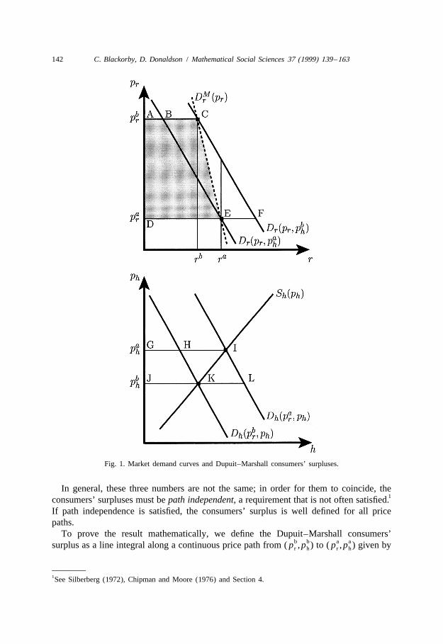
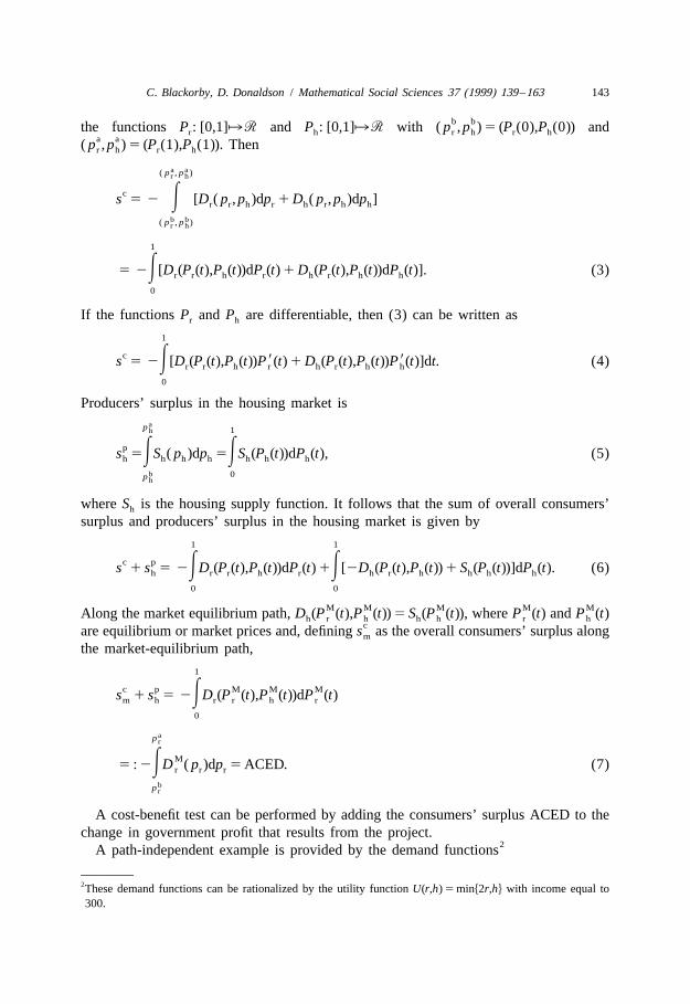
Before presenting our main general equilibrium result, we discuss the problem inpartial equilibrium. Following Sugden and Williams (1978), suppose that the govern-ment operates a rail service between a city and one of its suburbs, as illustrated in Fig. 1.
b aA project is planned which will reduce the price of rail trips from p to p (b stands forr r
‘before’, a stands for ‘after’). Cheaper transportation results in increased demand in the(competitive) suburban rental housing market, shifting the demand curve to the right—
b a bfrom D ( p , p ) to D ( p , p ). This results in an increase in the price of housing from ph r h h r h ha bto p which, in turn, shifts the demand curve for rail trips to the left—from D ( p , p ) toh r r h
aD ( p , p ). The initial equilibrium is at C and K, and the equilibrium after the change isr r h
at E and I.Dupuit–Marshall consumers’ surpluses can be measured in many different ways. If
cˆconsumers’ surplus in the rail market is calculated first, it is s 5 ACFD. Once p hasr rachanged, the relevant housing demand curve is D ( p , p ) and consumers’ surplus in theh r h
cˆhousing market is s 5 2 GILJ. Producers’ surplus (the increase in landlords’ profit) inhpthe housing market is s 5 GIKJ, and consumers’ surplus plus producers’ surplus inh
housing is
c p c c pˆ ˆ ˆs 1 s :5s 1 s 1 s 5 ACFD 2 GILJ 1 GIKJ 5 ACFD 2 ILK. (1)h r h h
Alternatively, the consumers’ surplus in housing can be computed first, and, in thisc b˜case, it is s 5 2 GHKJ, the area to the left of the original demand curve D ( p , p ).h h r h
aThe relevant demand curve for the rail-market surplus becomes D ( p , p ), andr r hc˜consumers’ surplus is s 5 ABED. Using this method, consumers’ surplus plusr
producers’ surplus in housing isc p c c c˜ ˜ ˜s 1 s :5s 1 s 1 s 5 ABED 2 GHKJ 1 GIKJ 5 ABED 1 HIK. (2)h r h h
A third method for calculating the surpluses can be obtained by considering a pricepath which reduces the price of rail trips, keeping the housing market in equilibrium.When this is done, price and quantity in the rail market move along the market demand
Mcurve D ( p ). The claim made by Hicks (1946a), (1946b) and by Sugden and Williamsr r
(1978) is that the area ACED to the left of the market demand curve is equal to theoverall consumers’ surplus plus producers’ surplus in the housing market. This can beseen intuitively by thinking of the change in p as a sequence of very small changes.r
This makes the ‘corrections’ 2ILK and HIK in (1) and (2) very small, and the sum ofconsumers’ surplus and producers’ surplus approaches ACED, the shaded area in Fig. 1.
142 C. Blackorby, D. Donaldson / Mathematical Social Sciences 37 (1999) 139 –163
Fig. 1. Market demand curves and Dupuit–Marshall consumers’ surpluses.
In general, these three numbers are not the same; in order for them to coincide, the1consumers’ surpluses must be path independent, a requirement that is not often satisfied.
If path independence is satisfied, the consumers’ surplus is well defined for all pricepaths.
To prove the result mathematically, we define the Dupuit–Marshall consumers’b b a asurplus as a line integral along a continuous price path from ( p , p ) to ( p , p ) given byr h r h
1See Silberberg (1972), Chipman and Moore (1976) and Section 4.
C. Blackorby, D. Donaldson / Mathematical Social Sciences 37 (1999) 139 –163 143
b bthe functions P : [0,1]∞5 and P : [0,1]∞5 with ( p , p ) 5 (P (0),P (0)) andr h r h r ha a( p , p ) 5 (P (1),P (1)). Thenr h r h
a a( p , p )r h
cs 5 2 E [D ( p , p )dp 1 D ( p , p )dp ]r r h r h r h h
b b( p , p )r h
1
5 2E[D (P (t),P (t))dP (t) 1 D (P (t),P (t))dP (t)]. (3)r r h r h r h h
0
If the functions P and P are differentiable, then (3) can be written asr h
1
c 9 9s 5 2E[D (P (t),P (t))P (t) 1 D (P (t),P (t))P (t)]dt. (4)r r h r h r h h
0
Producers’ surplus in the housing market isaph 1
ps 5ES ( p )dp 5ES (P (t))dP (t), (5)h h h h h h h
b 0ph
where S is the housing supply function. It follows that the sum of overall consumers’h
surplus and producers’ surplus in the housing market is given by
1 1
c ps 1 s 5 2ED (P (t),P (t))dP (t) 1E[2D (P (t),P (t)) 1 S (P (t))]dP (t). (6)h r r h r h r h h h h
0 0
M M M M MAlong the market equilibrium path, D (P (t),P (t)) 5 S (P (t)), where P (t) and P (t)h r h h h r hcare equilibrium or market prices and, defining s as the overall consumers’ surplus alongm
the market-equilibrium path,
1
c p M M Ms 1 s 5 2ED (P (t),P (t))dP (t)m h r r h r
0
ap r
M5 : 2ED ( p )dp 5 ACED. (7)r r r
bp r
A cost-benefit test can be performed by adding the consumers’ surplus ACED to thechange in government profit that results from the project.
2A path-independent example is provided by the demand functions
2These demand functions can be rationalized by the utility function U(r,h) 5 minh2r,hj with income equal to300.
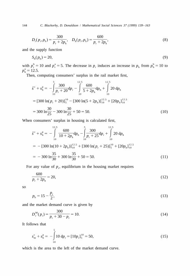
144 C. Blackorby, D. Donaldson / Mathematical Social Sciences 37 (1999) 139 –163
300 600]]] ]]]D ( p , p ) 5 , D ( p , p ) 5 , (8)r r h h r hp 1 2p p 1 2pr h r h
and the supply function
S ( p ) 5 20, (9)h h
b a bwith p 5 10 and p 5 5. The decrease in p induces an increase in p from p 5 10 tor r r h hap 5 12.5.h
Then, computing consumers’ surplus in the rail market first,
5 12.5 12.5
300 600c pˆ ]] ]]]s 1 s 5 2E dp 2 E dp 1 E 20 dph r h hp 1 20 5 1 2pr h10 10 10
10 12.5 12.55 [300 ln( p 1 20)] 2 [300 ln(5 1 2p )] 1 [20p ]r 5 h 10 h 10
30 30] ]5 300 ln 2 300 ln 1 50 5 50. (10)25 25
When consumers’ surplus in housing is calculated first,
12.5 5 12.5
600 300c p˜ ]]] ]]s 1 s 5 2 E dp 2E dp 1 E 20 dph h r h10 1 2p p 1 25h r10 10 10
12.5 10 12.55 2 [300 ln(10 1 2p )] 1 [300 ln( p 1 25)] 1 [20p ]h 10 r 5 h 10
35 35] ]5 2 300 ln 1 300 ln 1 50 5 50. (11)30 30
For any value of p , equilibrium in the housing market requiresr
600]]] 5 20, (12)p 1 2pr h
so
pr]p 5 15 2 , (13)h 2
and the market demand curve is given by
300M ]]]]D ( p ) 5 5 10. (14)r r p 1 30 2 pr r
It follows that5
c p 10s 1 s 5 2E10 dp 5 [10p ] 5 50, (15)m h r r 5
10
which is the area to the left of the market demand curve.
C. Blackorby, D. Donaldson / Mathematical Social Sciences 37 (1999) 139 –163 145
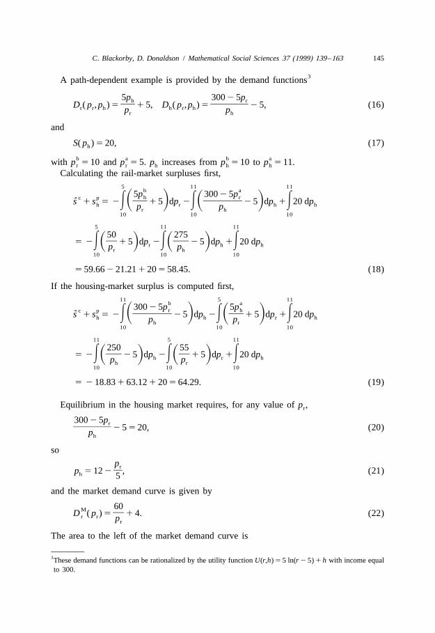
3A path-dependent example is provided by the demand functions
5p 300 2 5ph r] ]]]D ( p , p ) 5 1 5, D ( p , p ) 5 2 5, (16)r r h h r hp pr h
and
S( p ) 5 20, (17)h
b a b awith p 5 10 and p 5 5. p increases from p 5 10 to p 5 11.r r h h h
Calculating the rail-market surpluses first,5 11 11
b a5p 300 2 5ph rc pˆ ] ]]]s 1 s 5 2E 1 5 dp 2E 2 5 dp 1E20 dpS D S Dh r h hp pr h10 10 10
5 11 11
50 275] ]5 2E 1 5 dp 2E 2 5 dp 1E20 dpS D S Dr h hp pr h
10 10 10
5 59.66 2 21.21 1 20 5 58.45. (18)
If the housing-market surplus is computed first,11 5 11
b a300 2 5p 5pr hc p˜ ]]] ]s 1 s 5 2E 2 5 dp 2E 1 5 dp 1E20 dpS D S Dh h r hp ph r10 10 10
11 5 11
250 55] ]5 2E 2 5 dp 2E 1 5 dp 1E20 dpS D S Dh r hp ph r
10 10 10
5 2 18.83 1 63.12 1 20 5 64.29. (19)
Equilibrium in the housing market requires, for any value of p ,r
300 2 5pr]]]2 5 5 20, (20)ph
so
pr]p 5 12 2 , (21)h 5
and the market demand curve is given by
60M ]D ( p ) 5 1 4. (22)r r pr
The area to the left of the market demand curve is
3These demand functions can be rationalized by the utility function U(r,h) 5 5 ln(r 2 5) 1 h with income equalto 300.
146 C. Blackorby, D. Donaldson / Mathematical Social Sciences 37 (1999) 139 –163
5
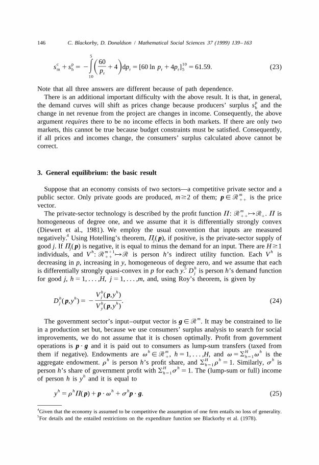
60c p 10]s 1 s 5 2E 1 4 dp 5 [60 ln p 1 4p ] 5 61.59. (23)S Dm h r r r 5pr10
Note that all three answers are different because of path dependence.There is an additional important difficulty with the above result. It is that, in general,
pthe demand curves will shift as prices change because producers’ surplus s and theh
change in net revenue from the project are changes in income. Consequently, the aboveargument requires there to be no income effects in both markets. If there are only twomarkets, this cannot be true because budget constraints must be satisfied. Consequently,if all prices and incomes change, the consumers’ surplus calculated above cannot becorrect.
3. General equilibrium: the basic result
Suppose that an economy consists of two sectors—a competitive private sector and ampublic sector. Only private goods are produced, m$2 of them; p [ 5 is the price11
vector.mThe private-sector technology is described by the profit function P : 5 ∞5 . P is11 1
homogeneous of degree one, and we assume that it is differentially strongly convex(Diewert et al., 1981). We employ the usual convention that inputs are measured
4negatively. Using Hotelling’s theorem, P ( p), if positive, is the private-sector supply ofj
good j. If P ( p) is negative, it is equal to minus the demand for an input. There are H $1jh m11 hindividuals, and V : 5 ∞5 is person h’s indirect utility function. Each V is11
decreasing in p, increasing in y, homogeneous of degree zero, and we assume that each5 his differentially strongly quasi-convex in p for each y. D is person h’s demand functionj
for good j, h 5 1, . . . ,H, j 5 1, . . . ,m, and, using Roy’s theorem, is given by
h hV ( p,y )jh h ]]]D ( p,y ) 5 2 . (24)j h hV ( p,y )y
mThe government sector’s input–output vector is g [ 5 . It may be constrained to liein a production set but, because we use consumers’ surplus analysis to search for socialimprovements, we do not assume that it is chosen optimally. Profit from governmentoperations is p ? g and it is paid out to consumers as lump-sum transfers (taxed from
h m H hthem if negative). Endowments are v [ 5 , h 5 1, . . . ,H, and v 5 o v is the1 h51h H h haggregate endowment. r is person h’s profit share, and o r 5 1. Similarly, s ish51
H hperson h’s share of government profit with o s 5 1. The (lump-sum or full) incomeh51hof person h is y and it is equal to
h h h hy 5 r P( p) 1 p ? v 1 s p ? g. (25)
4Given that the economy is assumed to be competitive the assumption of one firm entails no loss of generality.5For details and the entailed restrictions on the expenditure function see Blackorby et al. (1978).
C. Blackorby, D. Donaldson / Mathematical Social Sciences 37 (1999) 139 –163 147
1 H H hy 5 ( y , . . . ,y ) is the economy’s income vector and y 5 o y is aggregate income,h51
with
Hhy 5O y 5 P( p) 1 p ? v 1 p ? g. (26)
h51
Equilibrium requires, for each j 5 1, . . . ,m,
Hh hD ( p,y):5OD ( p,y ) 5 P ( p) 1 v 1 g . (27)j j j j j
h51
bWe consider a public project that moves the public input–output vector g from ga(before) to g (after). A path of integration is described by the continuous functions
m b a m bG: [0,1]∞5 , with g 5 G(0) and g 5 G(1), and P: [0,1]∞5 , with p 5 P(0) anda b a b ap 5 P(1). Equilibrium prices corresponding to g and g are p and p . The income
1 Hvector along the paths G and P is Y(t) 5 (Y (t), . . . ,Y (t)), t [ [0,1], and is given byb a(25) evaluated at g 5 G(t) and p 5 P(t) with y 5 Y(0) and y 5 Y(1). Aggregate income
H h b aalong the paths is Y(t) 5 o Y (t) with Y(0) 5 y and Y(1) 5 y , and is given by (26)h51
evaluated at g 5 G(t) and p 5 P(t).The Hicksian partial-equilibrium claim discussed in Section 2 above can be demon-
strated in this general equilibrium model. The aggregate Dupuit–Marshall consumers’surplus, allowing for income change, is
a a( p , y )m
s 5 E 2OD ( p,y)dp 1 dyF Gba j jj51
b b( p , y )
1m
5E 2OD (P(t),Y(t))dP (t) 1 dY(t) . (28)F Gj jj51
0
1 HIt is equal to the sum of the individual consumer’s surpluses s , . . . ,s , andba ba
a a( p , y )H H m
h h h hs 5O s 5O E 2OD ( p,y )dp 1 dyF Gba ba j jh51 h51 j51
b b( p , y )
1H m
h h h5OE 2OD (P(t),Y (t))dP (t) 1 dY (t) . (29)F Gj j
h51 j510
Theorem 1 shows that this consumers’ surplus can be computed in another way in anundistorted competitive economy: one in which all agents are price takers, producer andconsumer prices are equal, and all taxes and/or transfers are lump-sum. The generalequilibrium analogue to the market-demand-curve surplus of (7) is computed along aparticular path where all markets are in equilibrium. Along a market-equilibrium path,
M M 1M H MP(t) 5 P (t) and Y(t) 5 Y (t) 5 (Y (t), . . . ,Y (t)), where
148 C. Blackorby, D. Donaldson / Mathematical Social Sciences 37 (1999) 139 –163
HM M h M hMD (P (t),Y (t)) 5OD (P (t),Y (t))j j
h51
M5 P (P (t)) 1 v 1 G (t), (30)j j j
j 5 1, . . . ,m, for all G(t), t [ [0,1]. It is possible for these paths to be different even ifb athe end points g and g are the same because the paths hG(t)ut [ [0,1]j can be different,
t [ (0,1).
Theorem 1. For any market-equilibrium price path, the aggregate Dupuit–Marshallconsumers’ surplus (28) is equal to
1H m
h M a a b bs 5O s 5 2EOG (t)dP (t) 1 [ p ? g 2 p ? g ] (31)ba ba j jh51 j51
0
or, equivalently,
1H m
h Ms 5O s 5EOP (t)dG (t). (32)ba ba j jh51 j51
0
Proof. Along the market-equilibrium path, using (29) and (30) and noting that Y(t) 5H h b ao Y (t), Y(0) 5 y , and Y(1) 5 y ,h51
1H m
h M M M Ms 5O s 5E 2OD (P (t),Y (t))dP (t) 1 dY (t)F Gba ba j jh51 j51
0
1 1 1m m m
M M M M a b5 2EOP (P (t))dP (t) 2EOv dP (t) 2EOG (t)dP (t) 1 [y 2 y ]j j j j j j
j51 j51 j510 0 0
1m
a b a b M a b5 2 [P( p ) 2 P( p )] 2 [ p ? v 2 p ? v] 2EOG (t)dP (t) 1 [y 2 y ]. (33)j j
j510
Using (26), the change in income is
a b a b a b a a b by 2 y 5 [P( p ) 2 P( p )] 1 [ p ? v 2 p ? v] 1 [ p ? g 2 p ? g ], (34)
and (33) becomes
1m
M a a b bs 5 2EOG (t)dP (t) 1 [ p ? g 2 p ? g ], (35)ba j jj51
0
which is (31).Integrating (35) by parts yields
C. Blackorby, D. Donaldson / Mathematical Social Sciences 37 (1999) 139 –163 149
1m
a a b b M a a b bs 5 [ p ? g 2 p ? g ] 1EOP (t)dG (t) 2 [ p ? g 2 p ? g ], (36)ba j jj51
0
which yields (32). j
It is straightforward to interpret the results of Theorem 1. Eq. (31) is the generalequilibrium analogue of (7), the partial-equilibrium result. Because p ? g is government-
a a b bsector profit, [ p ? g 2 p ? g ] is the change in profit. It results in a change inconsumers’ incomes. The first term is easiest to interpret if the government sectorproduces a single good ( j51) with a change in its price but no change in the prices ofgovernment inputs (other prices may change). In that case, the surplus is simply
1
M a a b b2EG (t)dP (t) 1 [ p ? g 2 p ? g ]. (37)1 1
0
The first term corresponds to the area to the left of the market demand curve—ACED inFig. 1—and it should be added to the change in government-sector profit. Thesummation sign in (31) indicates that, in each market in which the governmentparticipates, consumers’ surpluses should be computed for each output or input whoseprice changes. It is true, of course, that there may be private-sector involvement in someor all of the goods (including inputs) that correspond to the non-zero elements of g. Eq.(31) indicates that this can be accounted for completely through the market equilibrium
Mpath hP (t)ut [ [0,1]j.Eq. (32) is an area under market demand curves. Suppose that some prices
b a ¯( j [ ^ # h1, . . . ,mj) are unaffected by the change in g, then p 5 p 5 p for thosej j ja b¯values of j, and the corresponding terms in (32) are o p [g 2 g ], the change inj[^ j j j
government-sector profit. If ^ 5 h1, . . . ,mj, this is the usual cost-benefit test in anundistorted competitive economy. In the case where all prices can change, it is possibleto approximate the path hP(t), t [ [0,1]j linearly with
P (t) 5 a G (t) 1 b , (38)j j j j
b aj 5 1, . . . ,m, P(0) 5 p , P(1) 5 p . In this case, (32) becomes
b ap 1 p a bF G]]s 5 ? [g 2 g ]. (39)ba 2b aThis is the change in government-sector profit computed at the average of p and p ,
before and after prices. Such averaging, based on partial-equilibrium arguments, iscommon in cost-benefit analysis and (39) provides a general-equilibrium justification.
4. Interpretation
In this section, we interpret the result of Theorem 1. Although it is interesting andpotentially useful, it is important to ask whether and under what conditions the
150 C. Blackorby, D. Donaldson / Mathematical Social Sciences 37 (1999) 139 –163
market-demand-curve surplus is an indicator of welfare change. To do that, weinvestigate it for all possible paths hG(t)ut [ [0,1]j and the corresponding paths h p 5
b aP(t)ut [ [0,1]j. We do not restrict the end points g 5 G(0) and g 5 G(1) and weassume, throughout the section, that individual incomes can move independently along
6 mmarket-equilibrium paths. It is not true that all possible price vectors p [ 5 are in11
some path. The results presented below do not depend on this, however. They are localresults and hold for feasible prices and incomes.
Because the demand functions are homogeneous of degree zero and because themarket-clearing equations only determine relative prices, many different normalizationsare possible: dividing by aggregate income, holding income equal to a constant, dividingby one price, and letting the sum of prices be constant. Of course, these normalizationsare mutually exclusive and, as we shall see, each leads to a different result. Eachsubsection below is devoted to one of them.
We use the following result from Courant (1936) on path independence of lineintegrals of the form
ax 1K K
k kEO f (x)dx 5EO f (X(t))dX (t), (40)k kk51 k51
b 0x
K K bx 5 (x , . . . ,x ) 5 (X (t), . . . ,X (t)) 5 X(t) [ 5 and X: [0,1]∞5 , with X(0) 5 x and1 K 1 KaX(1) 5 x . If the integral in (40) is path independent, then there must be a potential
a bfunction F such that it is equal to F(x ) 2 F(x ), and it must, therefore, be true that
K K≠F(x) k]]dF(x) 5O dx 5O f (x)dx (41)k k≠xkk51 k51
for all (dx , . . . ,dx ). This requires1 K
≠F(x) k]]5 f (x), (42)≠xk
k 5 1, . . . ,K, and, because
2 2≠ F(x) ≠ F(x)]] ]]5 , (43)≠x ≠x ≠x ≠xk l l k
k l≠f (x) ≠f (x)]] ]]5 (44)
≠x ≠xl k
for all x.
6A sufficient condition for this is that their endowment vectors are not co-linear.
C. Blackorby, D. Donaldson / Mathematical Social Sciences 37 (1999) 139 –163 151
4.1. No normalization
In this subsection, we normalize neither prices nor income and show that it isimpossible for the consumers’ surplus s , described by (31) or (32), to be pathba
independent for either a one- or a many-consumer economy. Theorem 2 was proved byChipman and Moore (1976) for one consumer.
Theorem 2. For any H $ 1, there are no well-behaved preferences such that s , givenba
by (28) or (29), is path independent.
Proof. Using (27), (28) and (29), the surplus can be rewritten as
a a( p , y )m H H
h h hs 5 E 2OOD ( p,y )dp 1Ody . (45)F Gba j jj51h51 h51
b b( p , y )
Path independence requires
H≠ ≠(1)h h] ]]OD ( p,y ) 5 5 0, (46)h j ≠p≠y jh51
or
≠ h h]D ( p,y ) 5 0 (47)h j≠y
for all h and all j which violates the regularity conditions on preferences. j
Path independence does not necessarily imply, however, that the aggregate consum-ers’ surplus s is consistent with a social-welfare function. We say that, for any H $ 1,ba
s is consistent with a Bergson–Samuelson social-welfare function if and only if therebaHexists an increasing function W : 5 ∞5 such that
a b 1a Ha 1b H bs $ 0↔W(u ) $ W(u )↔W(u , . . . ,u ) $ W(u , . . . ,u ) (48)ba
b 1b H bfor all alternatives B and A and all paths between them. u 5 (u , . . . ,u ) anda 1a Ha 7u 5 (u , . . . ,u ) are the utility vectors in B and A. If there is a single consumer, (48)
requires the surplus to be consistent with preferences. If s is consistent with aba
social-welfare function, it must be path independent (see Lemma 1 in Appendix A). Thisobservation together with Theorem 2 is sufficient for Corollary 2.1.
Corollary 2.1. For any H $ 1, there are no well-behaved preferences such that s isba
consistent with a Bergson–Samuelson social-welfare function.
7We use a social-welfare function for clarity of exposition. The existence of a social-welfare ordering of utilityvectors is sufficient.
152 C. Blackorby, D. Donaldson / Mathematical Social Sciences 37 (1999) 139 –163
This result suggests that, without normalizations of price(s) or income, the result ofTheorem 1 is nothing more than an intellectual curiosity.
4.2. Normalized prices
“In general equilibrium, only relative prices are determined and, if p is an equilibrium“price vector, so is lp for all l . 0. We consider first a one-consumer economy in which
prices along the equilibrium path can be divided by income without disturbingN 8equilibrium to create the normalized price path hP (t)ut [ [0,1]j, where
P (t) P (t)1 mN N N N ]] ]]p 5 P (t) 5 (P (t), . . . ,P (t)):5 , . . . , . (49)S D1 m Y(t) Y(t)
In this case the consumers’ surplus becomesNap
mN N Ns 5 2 EOD ( p ,1)dp . (50)ba j j
j51Nbp
Theorem 3. In a one-consumer economy, the consumer’s surplus in normalized pricesNs , given by (50), is path independent if and only if preferences are homothetic; that is,ba
* * Nu 5V( p,y) 5V(a( p)y) 5V(a( p )) (51)
*m11 mfor all ( p,y) [ 5 , where a : 5 ∞5 is homogeneous of degree minus one and V11 11
is increasing. In this case,N Na Nbs 5 ln a( p ) 2 ln a( p )ba
a a b b5 ln(a( p )y ) 2 ln(a( p )y )
21 21* *a b5 ln V (u ) 2 ln V (u ). (52)
Proof. Path independence and (50) imply
N N≠D ( p ,1) ≠D ( p ,1)j k]]] ]]]5 (53)N N
≠p ≠pk j
N mfor all j,k [ h1, . . . ,mj and all p [ 5 . For any y . 0,11
N≠D ( p,y) ≠D ( p ,1) 1j j]]] ]]]]5 (54)N≠p y≠pk k
for all j,k 5 1, . . . ,m, and (53) implies
8Mathematically, this is equivalent to requiring that Y(t) 5 1 for all t [ [0,1]. This result was proved bySilberberg (1972) and Chipman and Moore (1976).
C. Blackorby, D. Donaldson / Mathematical Social Sciences 37 (1999) 139 –163 153
≠D ( p,y) ≠D ( p,y)j k]]] ]]]5 (55)
≠p ≠pk j
m11for all j,k [ h1, . . . ,mj and all ( p,y) [ 5 . Therefore, the cross-partial derivatives of11
the uncompensated demand functions are symmetric, which implies homotheticity and(51) (Silberberg, 1972; Chipman and Moore, 1976). a is homogeneous of degree minus
hone because each V is homogeneous of degree zero.Given (51),
Na ( p )jN ]]D ( p ,1) 5 2 , (56)j Na( p )
Nj 5 1, . . . ,m. In this case, s becomesba
NapNm a ( p )jN N]]s 5 EO dpba N j
a( p )j51Nbp
Nap
N5 E d ln a( p )
Nbp
Na Nb5 ln(a( p )) 2 ln(a( p ))
a a b b5 ln(a( p )y ) 2 ln(a( p )y )
21 21* *a b5 ln V (u ) 2 ln V (u ). j (57)
Ns is an exact index of welfare change if and only if (51) is satisfied with normalizedba
prices which implies path independence. Accordingly, we have
Corollary 3.1. In a one-consumer economy, the consumer’s surplus in normalizedNprices s , given by (50), is an exact index of welfare change if and only if preferencesba
are homothetic and (51) is satisfied.
Although Theorem 3 and its corollary provide a possibility, it is a very restrictive one.Path independence requires symmetry of the cross-derivatives of the uncompensateddemand functions, which implies homotheticity. Consequently, the utility function isgiven by (51). Normalizing prices is equivalent to setting income equal to one,
m m2 o D ( p,1)dp 5 o a ( p) /a( p)dp 5 d ln a( p), and the logarithmic structure ofj51 j j j51 j j
(52) results.There is an analogue to Theorem 3 for many consumers. Equilibrium is consistent
with many normalizations and one of them allows us to choose aggregate income to beequal to one. In that case, prices are normalized by dividing by aggregate income and(49) applies. We show that this implies the existence of an aggregate consumer withhomothetic preferences. In addition, individual preferences must be either identical and
154 C. Blackorby, D. Donaldson / Mathematical Social Sciences 37 (1999) 139 –163
homothetic or quasi-homothetic and parallel. In the latter case, preferences mustaggregate to overall homotheticity.
˜The income vector y is defined by
1 Hy yS D˜ ] ]y 5 , . . . , (58)Y Y
H h˜and, because o y 5 1,h51
h 2 H˜ ˜ ˜ ˜y 5 1 2O y ,y , . . . ,y . (59)S Dh±1
The aggregate consumers’ surplus is written as
Na Na˜( p ,y )m H H
y h N h N h˜ ˜s 5 E 2OOD ( p ,y )dp 1OdyF Gba j jj51h51 h51
Nb Nb˜( p ,y )
Na Na˜( p ,y )m H
h N h N˜5 E 2OOD ( p ,y )dp . (60)F Gj jj51h51
Nb Nb˜( p ,y )
yTheorem 4. For H $ 2, the consumers’ surplus in normalized prices s , given by (60),ba
is path independent if and only if
h*h h h hV ( p,y ) 5V (a( p)y 1 b ( p)), (61)
m h mwhere a : 5 ∞5 is homogeneous of degree minus one, b : 5 ∞5 is homoge-11 11h* 9neous of degree zero, and V is increasing, h 5 1, . . . ,H. In addition,
hOb ( p) 5 constant. (62)h
yThe surplus s can be written asba
y Na Nbs 5 ln a( p ) 2 ln a( p )ba
a a b b5 ln(a( p )Y ) 2 ln(a( p )Y ).
H h 1 h˜ ˜ ˜Proof. Because o dy 5 0, dy 5 2 o dy , and (60) can be rewritten ash51 h±1
9Note that the function a is the same for each person.
C. Blackorby, D. Donaldson / Mathematical Social Sciences 37 (1999) 139 –163 155
Na a˜( p ,y )m
h N h 1 N h N h h˜ ˜ ˜ ˜E 2O OD ( p ,y ) 1 D p ,1 2O y dp 1Ody 2Ody .F S DGF Gj j jj51 h±1 h±1 h±1 h±1
Nb b˜( p ,y )
(64)
Path independence requires, for g ± 1,
≠ h N h 1 N h˜ ˜] OD ( p ,y ) 1 D p ,1 2O y 5 0 (65)F S DGg j j˜≠y h±1 h±1
or that
≠ g N g 1 N h˜ ˜] D ( p ,y ) 1 D p ,1 2O y 5 0. (66)F S DGg j j˜≠y h±1
This in turn implies that
≠ ≠g N g h N h˜ ˜] ][D ( p ,y )] 5 [D ( p ,y )] (67)g j h j˜≠y ˜≠y
for all g and h. Consequently,g g h hD ( p,y )Y 5 D ( p,y )Y (68)jy jy
org g h hD ( p,y ) 5 D ( p,y ), (69)jy jy
so that there must exist an aggregate consumer. It follows that the individual indirectutility functions can be written as in (61) (Gorman, 1953, 1961) with homogeneity
1 H 1 Hproperties of a and b , . . . ,b implied by homogeneity of degree zero of V , . . . ,V .˚The aggregate consumer’s utility function is V, with
H* hV̊( p,Y) 5V a( p)Y 1Ob ( p) . (70)S D
h51
yThe consumers’ surplus s is the surplus for the aggregate consumer (in normalizedba
prices). Path independence requires homotheticity by Theorem 3, and (62) results. Thesurplus is calculated as in Theorem 3. j
yIf s is consistent with a social-welfare function (48), path independence is implied.ba
Corollary 4.1 follows.
yCorollary 4.1. The consumers’ surplus in normalized prices s is consistent with aba
Bergson–Samuelson social-welfare function if and only if it is path-independent and(61) and (62) are satisfied, with
H H21h* h hW(u) 5OV (u ) 5 a( p) O y 1 constant. (71)S D
h51 h51
156 C. Blackorby, D. Donaldson / Mathematical Social Sciences 37 (1999) 139 –163
Corollary 4.1 indicates that the evaluator must be indifferent to inequality in thedistribution of income. The result of Theorem 4 and its corollary is connected to resultson social evaluation using the sum of compensating or equivalent variations inBlackorby and Donaldson (1985). Consistent aggregation is possible only when anaggregate consumer exists. As in the result above, evaluators must be indifferent toinequality in the distribution of income.
Eq. (61) requires each consumer to have quasi-homothetic preferences. Althoughh h h h¯there is a representation of the preferences of household h (V ( p,y ) 5 a( p)y 1 b ( p))
in which the marginal utility of income is independent of the level of income, it is not aconstant: because a is homogeneous of degree minus one, it must depend on at least oneprice. In addition, this property of the marginal utility of income is not shared by all ofthe (ordinally equivalent) representations of preferences.
4.3. Prices normalized to add to one
In this subsection, we normalize prices to add to one. This means that income andeach price must be divided by the sum of unadjusted prices along the path of integration.
hˇ ˇWriting the resulting prices and income as p and y , with
hp yh]]] ]]]ˇ ˇp 5 and y 5 , (72)m mO p O pi51 i i51 i
Sthe consumers’ surplus is equal to s , which is given byba
a aˇ ˇ( p ,y )m H
S hˇ ˇ ˇ ˇs 5 E 2OD (p,y )dp 1Ody . (73)F Gba j jj51 h51
b bˇ ˇ( p ,y )
Theorem 5. For any H $ 1, with prices and incomes normalized so that prices sum toSone, there are no well-behaved preferences such that s , given by (73), is pathba
independent.
m ˜ˇ ˇ ˇProof. Because o dp 5 0, writing p 5 (p , . . . ,p ),i51 i 2 m
a a˜ ˇ( p ,y )m H
S hˇ ˇ ˇ ˇ ˇ ˇs 5 E O[D (p,y ) 2 D (p,y )]dp 1Ody . (74)F Gba 1 j jj52 h51
b b˜ ˇ( p ,y )
Path independence requires
≠ ≠] ]ˇ ˇ ˇ ˇD (p,y ) 2 D (p,y ) 5 0, (75)h 1 h jˇ ˇ≠y ≠y
j ± 1, h 5 1, . . . ,H, and hence, using homogeneity of degree zero of the demandfunctions, that
C. Blackorby, D. Donaldson / Mathematical Social Sciences 37 (1999) 139 –163 157
≠ ≠h h h h] ]D ( p,y ) 5 D ( p,y ) (76)h 1 h j≠y ≠y
for all h and all j ± 1. The individual budget constraints imply thatm
≠ h h]Op D ( p,y ) 5 1, (77)j h j≠yj51
and, therefore, using (76),
≠ 1h h] ]]]D ( p,y ) 5 . (78)mh j≠y O pi51 i
Integrating,
hyh h hj]]]D ( p,y ) 5 1 f ( p) (79)mj O pi51 i
hjfor some function f . (79) and Roy’s theorem imply that
hyh h h h]]]˚u 5V ( p,y ) 5 1 c ( p), (80)mO pi51 i
h ˚where c is homogeneous of degree zero and 5 means ‘is ordinally equivalent to’.Consequently, there is an aggregate consumer. The demand functions can be written as
h myh h h h h]]] ˇ ˇD ( p,y ) 5 2 Op c ( p) 5 y 2 c (p ), (81)S Dmj i j ji51O pi51 i
h h H hwhere c is the jth partial derivative of c . Defining c( p) 5 o c ( p),j h51
Hhˇ ˇ ˇ ˇD (p,y ) 5O y 2 c (p ). (82)j j
h51
It follows thata aˇ ˇ( p ,y )
m HS hˇ ˇ ˇ ˇs 5 2 E O[c (p ) 2 c (p )]dp 1Ody , (83)ba 1 j j
j52 h51b bˇ ˇ( p ,y )
and path independence requires, for all j,k ± 1,
ˇ ˇ ˇ ˇc (p ) 2 c (p ) 5 c (p ) 2 c (p ), (84)1j kj 1k jk
and, therefore,
ˇ ˇc (p ) 5 c (p ). (85)1j 1k
ˇBecause (85) holds for all p and all j,k ± 1, there exist functions d and e such that
158 C. Blackorby, D. Donaldson / Mathematical Social Sciences 37 (1999) 139 –163
m
ˇ ˇ ˇ ˇc (p ) 5 d(p ) Op 1 e(p ). (86)S D1 1 i 1i52
m ˇBecause o p 5 1,i51 i
ˇ ˇ ˇ ˇc (p ) 5 d(p )(1 2 p ) 1 e(p ), (87)1 1 1 1
ˇwhich is a function of p alone. Because c is homogeneous of degree zero, c is1 1
homogeneous of degree minus one, and it follows that
l1]ˇc (p ) 5 , (88)1 p̌1
where l is an arbitrary constant.1
Although good one was chosen in the argument above to be the residual commodity,any good can play that role and, therefore, (88) generalizes to all goods with
l j]ˇc (p ) 5 , (89)j p̌ j
j 5 1, . . . ,m. Because c is homogeneous of degree minus one,j
m ˇc (p ) l lj j j]]] ]]]] ]ˇc ( p) 5 c Op p 5 5 5 (90)SS D D m mj j i pji51 ˇO p O p ps di51 i i51 i j
for all j and, integrating,
m
c( p) 5Ol ln p 1 g, (91)j jj51
mwhere g is a constant. Because c is homogeneous of degree zero, o l 5 0.j51 j
Now consider the case m 5 2. There is an aggregate consumer with preferencesrepresented by
Y]]˚V( p,Y) 5 1 l ln p 2 l ln p . (92)1 2p 1 p1 2
If l 5 0, our curvature assumption is violated. Without loss of generality, let l . 0. Theexpenditure function corresponding to V is E, with
E(u, p) 5 ( p 1 p )(u 2 l ln p 1 l ln p ). (93)1 2 1 2
Given this,
l( p 2 p )1 2]]]E (u, p) 5 2 , (94)11 2( p )1
and our assumptions require it to be negative for all (u, p). But, because it is positivewhen p . p , an impossibility results. j2 1
SIt is also impossible for the consumers’ surplus s to be consistent with a Bergson–ba
C. Blackorby, D. Donaldson / Mathematical Social Sciences 37 (1999) 139 –163 159
Samuelson social-welfare function because that requires the integral in (73) to be pathindependent. This observation proves
SCorollary 5.1. For any H $ 1, there are no well-behaved preferences such that s isba
consistent with a Bergson–Samuelson social-welfare function.
´4.4. A numeraire good
´It is also possible to choose some good as a numeraire, normalizing its price to one. Ifh h¯ ¯good k is chosen, prices and income become p 5 p /p , j 5 1, . . . ,m, and y 5 y /p .j j k k
1 H¯ ¯ ¯Letting y 5 (y , . . . ,y ) 5 y /p , consumers’ surplus isk
a a¯ ¯( p ,y )2kH
k h¯ ¯ ¯ ¯ ¯s 5 E 2OD (p,y )dp 1Ody , (95)F Gba j jj±k h51
b b¯ ¯( p ,y )2k
¯ ¯where p is p without its kth element. Theorem 6 characterizes preferences that allow2kks̄ to be path independent.ba
´Theorem 6. For any H $ 1, if good k [ h1, . . . ,mj is chosen as numeraire, thek¯consumers’ surplus s , given by (95), is path independent if and only if the individualba
indirect utility functions can be written as
h hh y 1 c ( p)*h h ]]]]V ( p,y ) 5V , (96)S Dpk
h*hwhere c is homogeneous of degree one and V is increasing, h 5 1, . . . ,H. The surplus
is given by
H H Hk kh ha h a hb h b¯ ¯ ¯ ¯ ¯ ¯s 5O s 5O (y 1 c (p )) 2O (y 1 c (p ))ba ba
h51 h51 h51
H ha h a H hb h by 1 c ( p ) y 1 c ( p )]]]] ]]]]5O 2O . (97)S Da S Dbp ph51 h51k k
Proof. The surplus can be written as
a a¯ ¯( p ,y )2kH H
k h h¯ ¯ ¯ ¯ ¯s 5 E 2O OD (p,y )dp 1Ody , (98)F Gba j jj±k h51 h51
b b¯ ¯( p ,y )2k
and path independence requiresH
≠ ≠ ≠(1)h g h] ¯ ¯ ] ¯ ¯ ]]OD (p,y ) 5 D (p,y ) 5 5 0 (99)g gj j ¯≠p¯ ¯≠y ≠y jh51
¯ ¯for all g, j ± k, p, y. Therefore, for each h and each j ± k,
160 C. Blackorby, D. Donaldson / Mathematical Social Sciences 37 (1999) 139 –163
≠ h h]D ( p,y ) 5 0, (100)h j≠y
hbecause D is homogeneous of degree zero. By Hotelling’s theorem,j
≠h h h h h]D ( p,y ) 5 E (V ( p,y ), p), (101)j ≠pj
h hwhere E is the expenditure function corresponding to V . Eqs. (100) and (101) imply
h hE (u , p) 5 0 (102)ju
or, equivalently,
h hE (u , p) 5 0 (103)uj
hfor all (u , p) and all j ± k. Integrating, and taking account of the fact that (103) holds forall j ± k and that the expenditure function and its utility derivative are homogeneous ofdegree one in prices,
h h h h¯¯E (u ,p ) 5 f (u , p )u k
h h¯5 p f (u ,1)k
h h5 :p f (u ) (104)k
hfor some function f . Integrating again yields
h h h h hE (u , p) 5 p f (u ) 2 c ( p) (105)k
h h h h hfor functions f and c . Setting E (u , p) 5 y and inverting yields
h hh y 1 c ( p)*h h ]]]]V ( p,y ) 5V , (106)S Dpk
h hwhich is (96). For each h, c must be homogeneous of degree one because V ishomogeneous of degree zero.
Given (106),
h h h¯ ¯ ¯D (p,y ) 5 2 c (p ), (107)j j
j ± k. Then, the surplus of consumer h is given by
a ha¯ ¯( p ,y )2k
kh h h¯ ¯ ¯ ¯s 5 E Oc (p )dp 1 dyF Gba j jj±k
b hb¯ ¯( p ,y )2k
C. Blackorby, D. Donaldson / Mathematical Social Sciences 37 (1999) 139 –163 161
a ha¯ ¯( p ,y )2k
h h¯ ¯5 E [dc (p ) 1 dy ]b hb¯ ¯( p ,y )2k
ha h a hb h b¯ ¯ ¯ ¯5 [y 1 c (p )] 2 [y 1 c (p )]. (108)
k H kh¯ ¯Because s 5 o s , the aggregate surplus is given by (97). jba h51 ba
It follows immediately from Theorem 6 that
k¯Corollary 6.1. For any H $ 1, the consumers’ surplus s is consistent with aba
Bergson–Samuelson social-welfare function if and only if (96) holds and the social-welfare function W is given by
H21h* h˚W(u) 5OV (u ). (109)
h51
´The indirect utility functions in (96) have no income effects for non-numeraire goods.Because of this, the aggregate Dupuit–Marshall consumers’ surplus is the same as theaggregate of the Hicksian compensating and equivalent variations. In addition, as in
h h h˜Section 4.2, there is a representation of each household’s preferences (V ( p,y ) 5 ( y 1h
c ( p)) /p ) such that the marginal utility of income is independent of the level ofk
income. But it is not constant because it depends on p . This property is not shared by allk
of the representations of households’ preferences. It is true, of course, that theDupuit–Marshall consumers’ surpluses depend on household demand functions and,because of this, are unaffected by applications of increasing transformations to utilityfunctions. Consequently, any attempt to characterize necessary or sufficient conditionsfor consistent aggregation in terms of marginal utilities of income is both misleading andmeaningless.
´Each choice of numeraire good results in different preferences and a differentsocial-welfare function. Because consumers must have different preferences for different
´choices of numeraire, this result is unsatisfactory. In each case, however, the evaluatormust be indifferent to inequality in the distribution of income.
5. Conclusion
We have extended the claim of Hicks that the aggregate Dupuit–Marshall consumers’surplus associated with the market demand curve(s) is equal to the consumers’ surplus inall markets together with producers’ surpluses in other markets in partial and generalequilibrium in an undistorted economy. This attractive result can be used to justify acost-benefit test which simply computes project profitability at the average of before-and after-project prices.
There are difficulties with this result in cost-benefit analysis, however. Withoutnormalization, the surplus can be path dependent and, as a consequence, cannot be
162 C. Blackorby, D. Donaldson / Mathematical Social Sciences 37 (1999) 139 –163
consistent with a Bergson–Samuelson social-welfare function. Possibilities arise only´when normalized prices (prices divided by aggregate income) or a numeraire are
employed. In the first case, an aggregate consumer with homothetic preferences isrequired. In the second, there is an aggregate consumer, income effects for each person
´are confined to the numeraire, and preferences must be different for different choices of´ ´numeraire. Because of this, a project may pass the cost-benefit test using one numeraire
and fail it using another. But preferences are supposed to be primitives in economicmodels; choosing them to accommodate an arbitrary price normalization is not in thespirit of the cost-benefit enterprise. All of these results suggest that the Dupuit–Marshallconsumers’ surplus methodology that pervades cost-benefit analysis is theoreticallyunsatisfactory.
Acknowledgements
Financial support through a grant from the Social Sciences and Humanities ResearchCouncil of Canada is gratefully acknowledged. We are indebted to a referee and anAssociate Editor for helpful comments. Earlier versions of the paper were presented atDalhousie University, the University of Nottingham, and the University of BritishColumbia. We thank the participants for their comments.
Appendix A
Lemma 1. The line integralax
mkEO f (x)dx (A.1)k
k51bx
satisfiesax
mk a bEO f (x)dx $ 0↔F(x ) $ F(x ) (A.2)k
k51bx
mfor all continuous paths in 6 # 5 and some function F : 6 ∞5 if and only if it ispath-independent.
b a ¯ ˆ ˆProof. Consider, for any x , x [ 6, any two paths C and C. Define C 9 as the reverse ofa b b a b˜ˆ ¯ ˆC (from x to x ) and C as the path from x to x along C and back to x along C 9. Eq.
(A.2) implies that the line integral must be zero on any closed path (from any x toitself). Therefore,
m m mk k kEO f (x)dx 5EO f (x)dx 1EO f (x)dxk k k
k51 k51 k51¯˜ ˆC C 9C
C. Blackorby, D. Donaldson / Mathematical Social Sciences 37 (1999) 139 –163 163
m mk k
5EO f (x)dx 2EO f (x)dx 5 0. (A.3)k kk51 k51
¯ ˆC C
Consequently,
m mk kEO f (x)dx 5EO f (x)dx , (A.4)k k
k51 k51¯ ˆC C
and the integral is path-independent.b aIf the integral is path-independent, for all paths between x and x ,
axm
k a bEO f (x)dx 5 G(x ) 2 G(x ) (A.5)kk51
bx
for some function G: 6 ∞5 and (A.2) is satisfied. j
References
Dupuit, J., 1969. On the measurement of the utility of public works. In: Arrow, K., Scitovsky, T. (Eds.),Readings in Welfare Economics (Barback, R.H., Trans.). Irwin, Homewood, pp. 255–283 (original workpublished 1844).
Marshall, A., 1920. Principles of Economics: An Introductory Volume, 8th ed. Macmillan, London (originalwork published 1890).
´ ˆ ´Hicks, J., 1946a. L’economie de bien-etre et la theorie des surplus du consommateur. Bulletin de l’Institut de´Sciences Economique Appliquee 2, 1–17.
´Hicks, J., 1946b. Quelques applications de la theorie des surplus du consommateur. Bulletin de l’Institut de´Sciences Economique Appliquee 2, 18–28.
Sugden, R., Williams, A., 1978. The Principles of Practical Cost-Benefit Analysis. Oxford University Press,Oxford.
Silberberg, E., 1972. Duality and the many consumer’s surpluses. American Economic Review 62, 942–956.Chipman, J., Moore, J., 1976. The scope of consumer’s surplus arguments. In: Tang, M., Westfield, F., Worley,
J. (Eds.), Welfare and Time in Economics: Essays in Honor of Nicholas Georgescu-Roegen. Heath,Lexington, pp. 69–123.
Diewert, W., Avriel, M., Zang, I., 1981. Nine kinds of quasiconcavity and concavity. Journal of EconomicTheory 25, 397–420.
Blackorby, C., Primont, D., Russell, R.R., 1978. Duality, Separability and Functional Structure: Theory andEconomic Applications. North-Holland/American Elsevier, Amsterdam/New York.
Courant, R., 1936. Differential and Integral Calculus, Vol. II. Wiley-Interscience, New York.Gorman, W., 1953. Community preference fields. Econometrica 21, 63–80 (reprinted in: Blackorby, C.,
Shorrocks, A. (Eds.), 1995. Separability and Aggregation: Vol. 1, Collected Works of W.M. Gorman.Clarendon, Oxford).
Gorman, W., 1961. On a class of preference fields. Metroeconomica 13, 53–56 (reprinted in: Blackorby, C.,Shorrocks, A. (Eds.), 1995. Separability and Aggregation: Vol. 1, Collected Works of W.M. Gorman.Clarendon, Oxford).
Blackorby, C., Donaldson, D., 1985. Consumers’ surpluses and consistent cost-benefit tests. Social Choice andWelfare 1, 251–262.