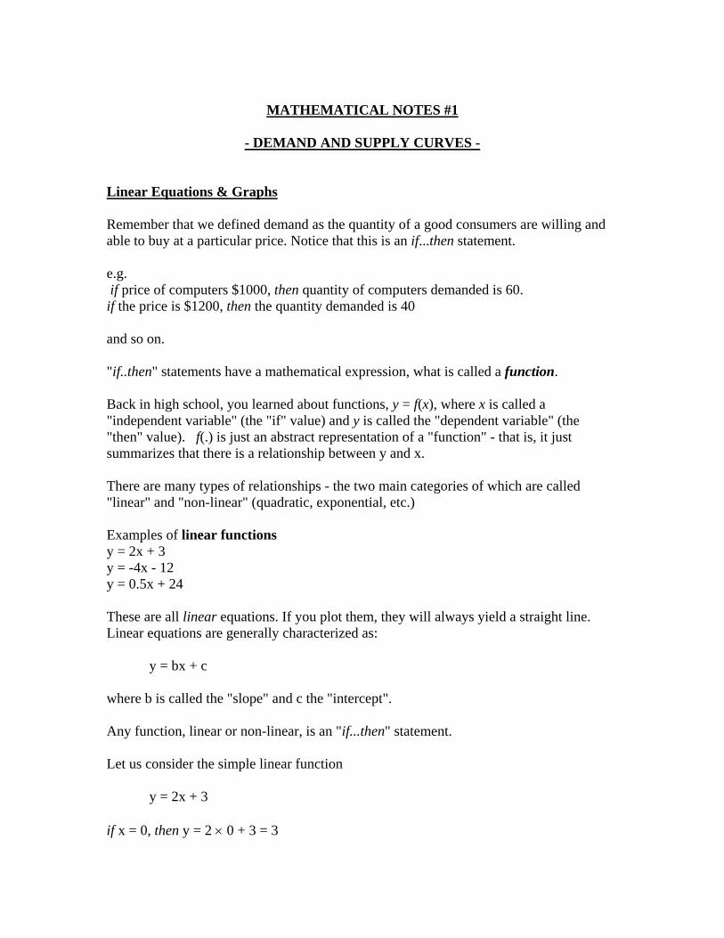
MATHEMATICAL NOTES #1

- DEMAND AND SUPPLY CURVES -

Linear Equations & Graphs Remember that we defined demand as the quantity of a good consumers are willing and able to buy at a particular price. Notice that this is an if...then statement. e.g. if price of computers $1000, then quantity of computers demanded is 60. if the price is $1200, then the quantity demanded is 40 and so on. "if..then" statements have a mathematical expression, what is called a function. Back in high school, you learned about functions, y = f(x), where x is called a "independent variable" (the "if" value) and y is called the "dependent variable" (the "then" value). f(.) is just an abstract representation of a "function" - that is, it just summarizes that there is a relationship between y and x. There are many types of relationships - the two main categories of which are called "linear" and "non-linear" (quadratic, exponential, etc.) Examples of linear functions y = 2x + 3 y = -4x - 12 y = 0.5x + 24 These are all linear equations. If you plot them, they will always yield a straight line. Linear equations are generally characterized as: y = bx + c where b is called the "slope" and c the "intercept". Any function, linear or non-linear, is an "if...then" statement. Let us consider the simple linear function y = 2x + 3 if x = 0, then y = 2 × 0 + 3 = 3

2

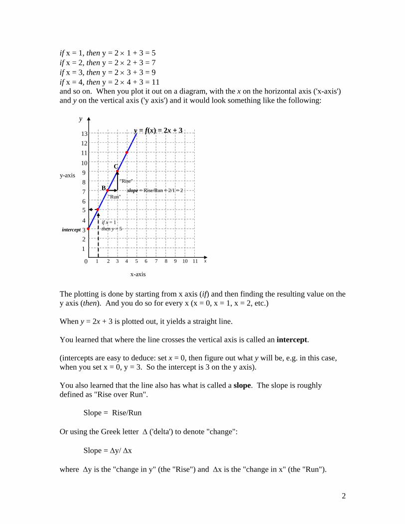
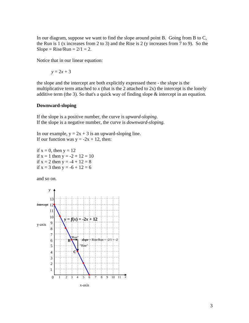
if x = 1, then y = 2 × 1 + 3 = 5 if x = 2, then y = 2 × 2 + 3 = 7 if x = 3, then y = 2 × 3 + 3 = 9 if x = 4, then y = 2 × 4 + 3 = 11 and so on. When you plot it out on a diagram, with the x on the horizontal axis ('x-axis') and y on the vertical axis ('y axis') and it would look something like the following:

1 2 3 4

5 6 7 8 9 10

1 2 3 4 5 6 7 8 9 10

y-axis

0 11

•

"Rise"

"Run"

C

y = f(x) = 2x + 3

11 12 13

x

y

x-axis

•

•

•

•

slope = Rise/Run = 2/1 = 2

intercept

if x = 1 then y = 5

B

The plotting is done by starting from x axis (if) and then finding the resulting value on the y axis (then). And you do so for every x (x = 0, x = 1, x = 2, etc.) When y = 2x + 3 is plotted out, it yields a straight line. You learned that where the line crosses the vertical axis is called an intercept. (intercepts are easy to deduce: set x = 0, then figure out what y will be, e.g. in this case, when you set x = 0, y = 3. So the intercept is 3 on the y axis). You also learned that the line also has what is called a slope. The slope is roughly defined as "Rise over Run". Slope = Rise/Run Or using the Greek letter Δ ('delta') to denote "change": Slope = Δy/ Δx where Δy is the "change in y" (the "Rise") and Δx is the "change in x" (the "Run").

3

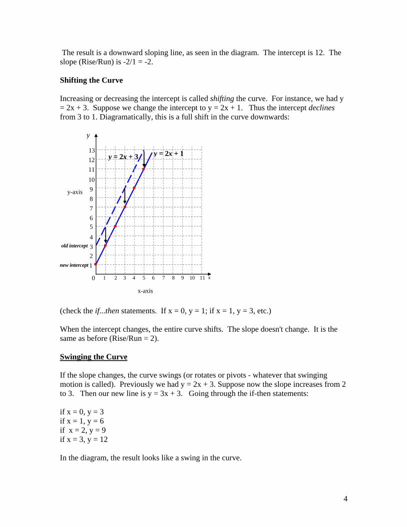
In our diagram, suppose we want to find the slope around point B. Going from B to C, the Run is 1 (x increases from 2 to 3) and the Rise is 2 (y increases from 7 to 9). So the Slope = Rise/Run = 2/1 = 2. Notice that in our linear equation: y = 2x + 3 the slope and the intercept are both explicitly expressed there - the slope is the multiplicative term attached to x (that is the 2 attached to 2x) the intercept is the lonely additive term (the 3). So that's a quick way of finding slope & intercept in an equation. Downward-sloping If the slope is a positive number, the curve is upward-sloping. If the slope is a negative number, the curve is downward-sloping. In our example, y = 2x + 3 is an upward-sloping line. If our function was y = -2x + 12, then: if x = 0, then y = 12 if x = 1 then y = -2 + 12 = 10 if x = 2 then y = -4 + 12 = 8 if x = 3 then y = -6 + 12 = 6 and so on.

1 2 3 4

5 6 7 8 9 10

1 2 3 4 5 6 7 8 9 10

y-axis

0 11

• "Rise"

"Run"

C

y = f(x) = -2x + 12

11 12 13

x

y

x-axis

•

•

•

•

slope = Rise/Run = -2/1 = -2

intercept

B

•

•

4

The result is a downward sloping line, as seen in the diagram. The intercept is 12. The slope (Rise/Run) is -2/1 = -2. Shifting the Curve Increasing or decreasing the intercept is called shifting the curve. For instance, we had y = 2x + 3. Suppose we change the intercept to y = 2x + 1. Thus the intercept declines from 3 to 1. Diagramatically, this is a full shift in the curve downwards:

1 2 3 4 5 6 7 8 9 10

1 2 3 4 5 6 7 8 9 10

y-axis

0 11

•

y = 2x + 3

11 12 13

x

y

x-axis

•

•

•

new intercept

y = 2x + 1

•

• old intercept

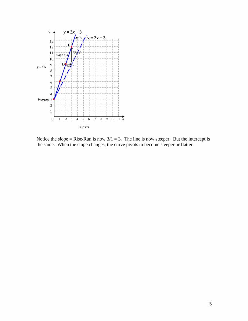
(check the if...then statements. If x = 0, y = 1; if x = 1, y = 3, etc.) When the intercept changes, the entire curve shifts. The slope doesn't change. It is the same as before (Rise/Run = 2). Swinging the Curve If the slope changes, the curve swings (or rotates or pivots - whatever that swinging motion is called). Previously we had y = 2x + 3. Suppose now the slope increases from 2 to 3. Then our new line is y = 3x + 3. Going through the if-then statements: if x = 0, y = 3 if x = 1, y = 6 if x = 2, y = 9 if x = 3, y = 12 In the diagram, the result looks like a swing in the curve.

5

1 2 3 4 5 6 7 8 9 10

1 2 3 4 5 6 7 8 9 10

y-axis

0 11

•

"Rise"

"Run"

y = 2x + 3

11 12 13

x

y

x-axis

slope = 3

intercept

D

•

•

•

E

y = 3x + 3

Notice the slope = Rise/Run is now 3/1 = 3. The line is now steeper. But the intercept is the same. When the slope changes, the curve pivots to become steeper or flatter.

6

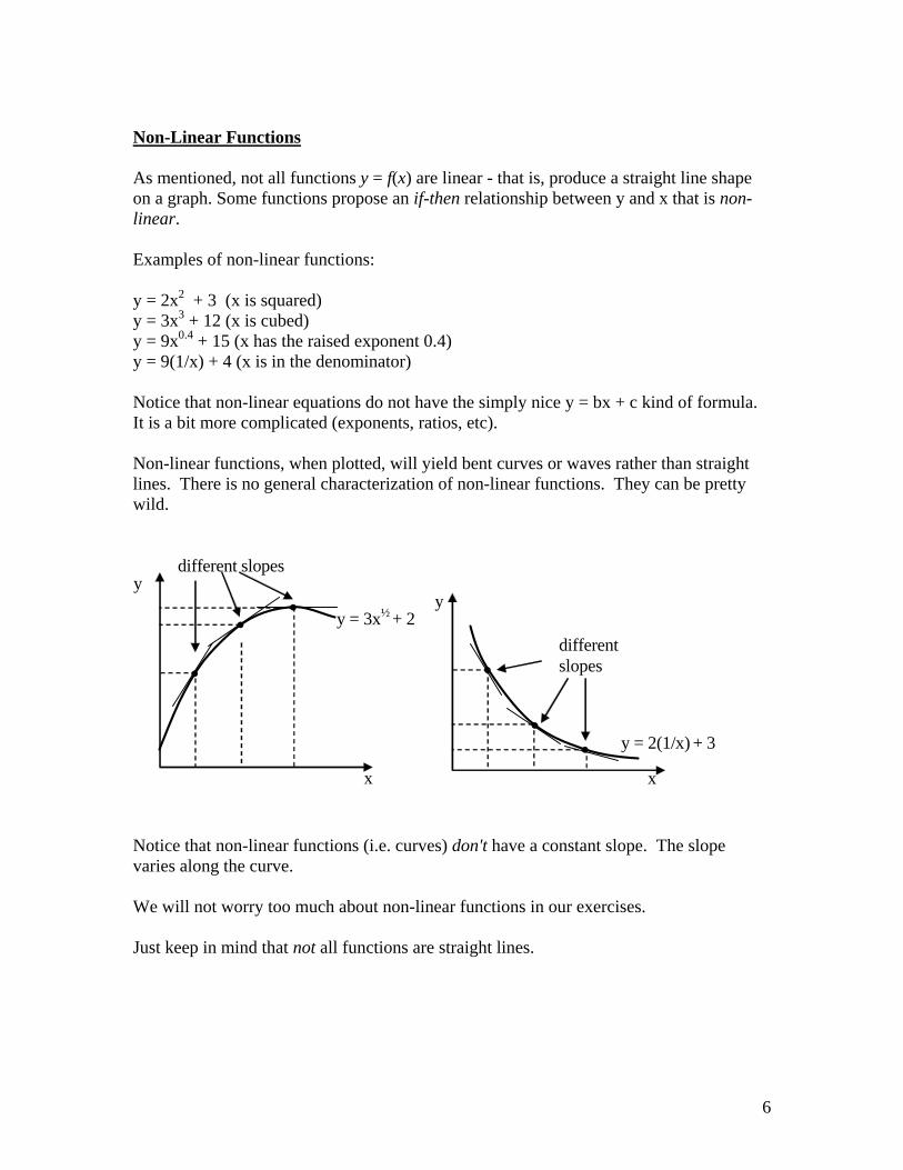
Non-Linear Functions As mentioned, not all functions y = f(x) are linear - that is, produce a straight line shape on a graph. Some functions propose an if-then relationship between y and x that is non-linear. Examples of non-linear functions: y = 2x2 + 3 (x is squared) y = 3x3 + 12 (x is cubed) y = 9x0.4 + 15 (x has the raised exponent 0.4) y = 9(1/x) + 4 (x is in the denominator) Notice that non-linear equations do not have the simply nice y = bx + c kind of formula. It is a bit more complicated (exponents, ratios, etc). Non-linear functions, when plotted, will yield bent curves or waves rather than straight lines. There is no general characterization of non-linear functions. They can be pretty wild.

x

y = 3x½ + 2

y

•

• •

different slopes

x

y = 2(1/x) + 3

y

•

• •

different slopes

Notice that non-linear functions (i.e. curves) don't have a constant slope. The slope varies along the curve. We will not worry too much about non-linear functions in our exercises. Just keep in mind that not all functions are straight lines.

7

DEMAND CURVES

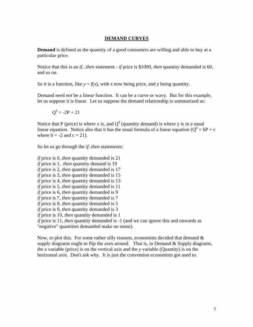
Demand is defined as the quantity of a good consumers are willing and able to buy at a particular price. Notice that this is an if...then statement - if price is $1000, then quantity demanded is 60, and so on. So it is a function, like y = f(x), with x now being price, and y being quantity. Demand need not be a linear function. It can be a curve or wavy. But for this example, let us suppose it is linear. Let us suppose the demand relationship is summarized as: Qd = -2P + 21 Notice that P (price) is where x is, and Qd (quantity demand) is where y is in a usual linear equation. Notice also that it has the usual formula of a linear equation (Qd = bP + c where b = -2 and c = 21). So let us go through the if..then statements: if price is 0, then quantity demanded is 21 if price is 1, then quantity demand is 19 if price is 2, then quantity demanded is 17 if price is 3, then quantity demanded is 15 if price is 4, then quantity demanded is 13 if price is 5, then quantity demanded is 11 if price is 6, then quantity demanded is 9 if price is 7, then quantity demanded is 7 if price is 8, then quantity demanded is 5 if price is 9, then quantity demanded is 3 if price is 10, then quantity demanded is 1 if price is 11, then quantity demanded is -1 (and we can ignore this and onwards as "negative" quantities demanded make no sense). Now, to plot this. For some rather silly reasons, economists decided that demand & supply diagrams ought to flip the axes around. That is, in Demand & Supply diagrams, the x variable (price) is on the vertical axis and the y variable (Quantity) is on the horizontal axis. Don't ask why. It is just the convention economists got used to.

8

1 2 3 4

5 6 7 8 9 10

1 2 3 4 5 6 7 8 9 10

x-axis

0 11

"Rise"

"Run"

C

Q = -2P + 21

11 12 13

Quantity

Price

y-axis

• •

slope = Rise/Run = -1/2

intercept

B

• 12 13 14 15 16 17 18 19 20 21 22

• •

• •

• •

• •

Demand Curve

if Price = 2....

...then Quantity = 17....

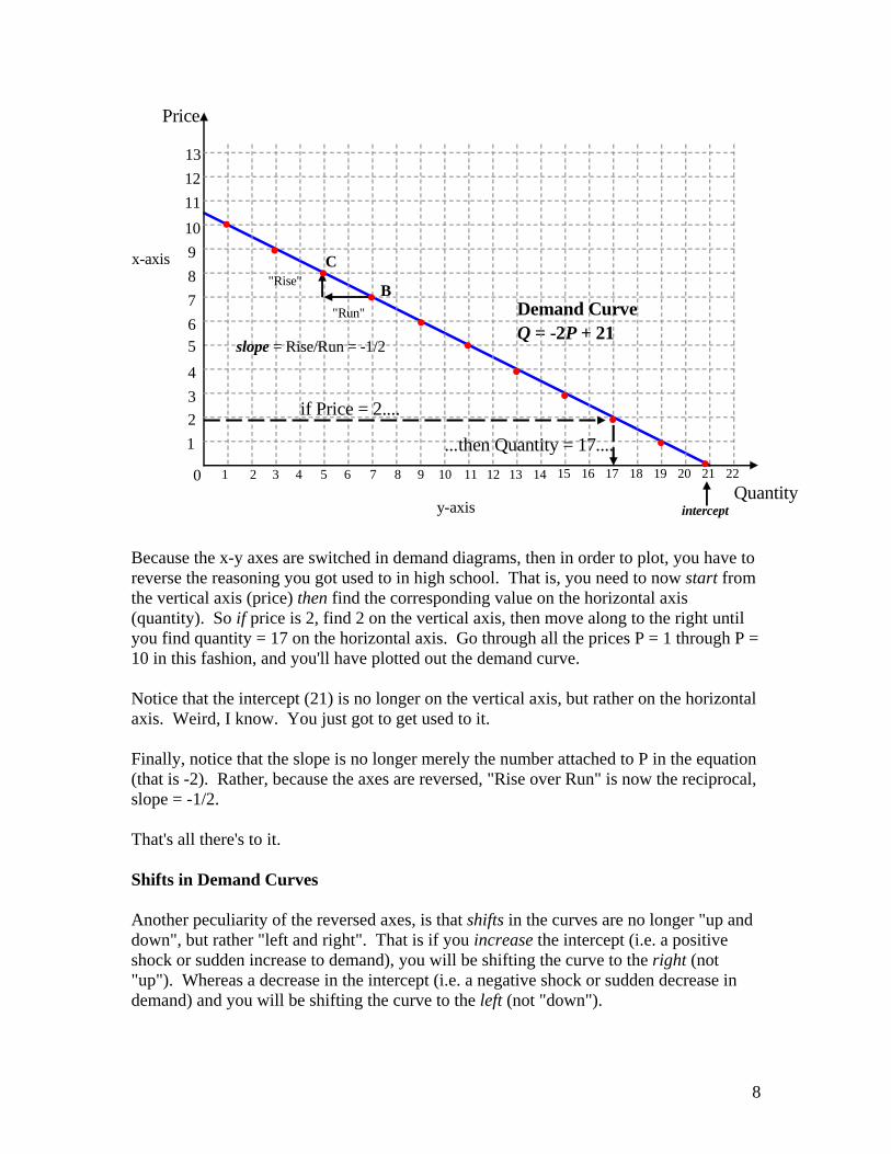
Because the x-y axes are switched in demand diagrams, then in order to plot, you have to reverse the reasoning you got used to in high school. That is, you need to now start from the vertical axis (price) then find the corresponding value on the horizontal axis (quantity). So if price is 2, find 2 on the vertical axis, then move along to the right until you find quantity = 17 on the horizontal axis. Go through all the prices P = 1 through P = 10 in this fashion, and you'll have plotted out the demand curve. Notice that the intercept (21) is no longer on the vertical axis, but rather on the horizontal axis. Weird, I know. You just got to get used to it. Finally, notice that the slope is no longer merely the number attached to P in the equation (that is -2). Rather, because the axes are reversed, "Rise over Run" is now the reciprocal, slope = -1/2. That's all there's to it. Shifts in Demand Curves Another peculiarity of the reversed axes, is that shifts in the curves are no longer "up and down", but rather "left and right". That is if you increase the intercept (i.e. a positive shock or sudden increase to demand), you will be shifting the curve to the right (not "up"). Whereas a decrease in the intercept (i.e. a negative shock or sudden decrease in demand) and you will be shifting the curve to the left (not "down").

9

Q

P A positive shock to demand

right is more

Q

P A negative shock to demand

left is less The mnemonic device "less is left" maybe a way to remember that. When does a demand curve shift? Anything that causes an increase or decrease in demand for a good (except for a change in the price of the good itself) will lead to a shift the demand curve. Examples of what can cause a shock in demand (a shift): - increase or decrease in popular taste for a good - increase or decrease in people's incomes - lower price of a substitute good (e.g. lower price of tea causes a decrease in demand for coffee (a natural substitute for tea), thus there will be a shift left in demand for coffee). - higher price for a substitute good (e.g. higher price of tea causes an increase in demand for coffee, thus shift right in demand for coffee). Why is all this a shift? Because all these things increase demand for a good regardless of the exact price. e.g. Price Old Quantity

Demanded New Quantity Demanded

10 1 4 9 3 6 8 5 8 7 7 10 6 9 12 5 11 14 4 13 16 3 15 18 2 17 20 1 19 22 0 21 24

10

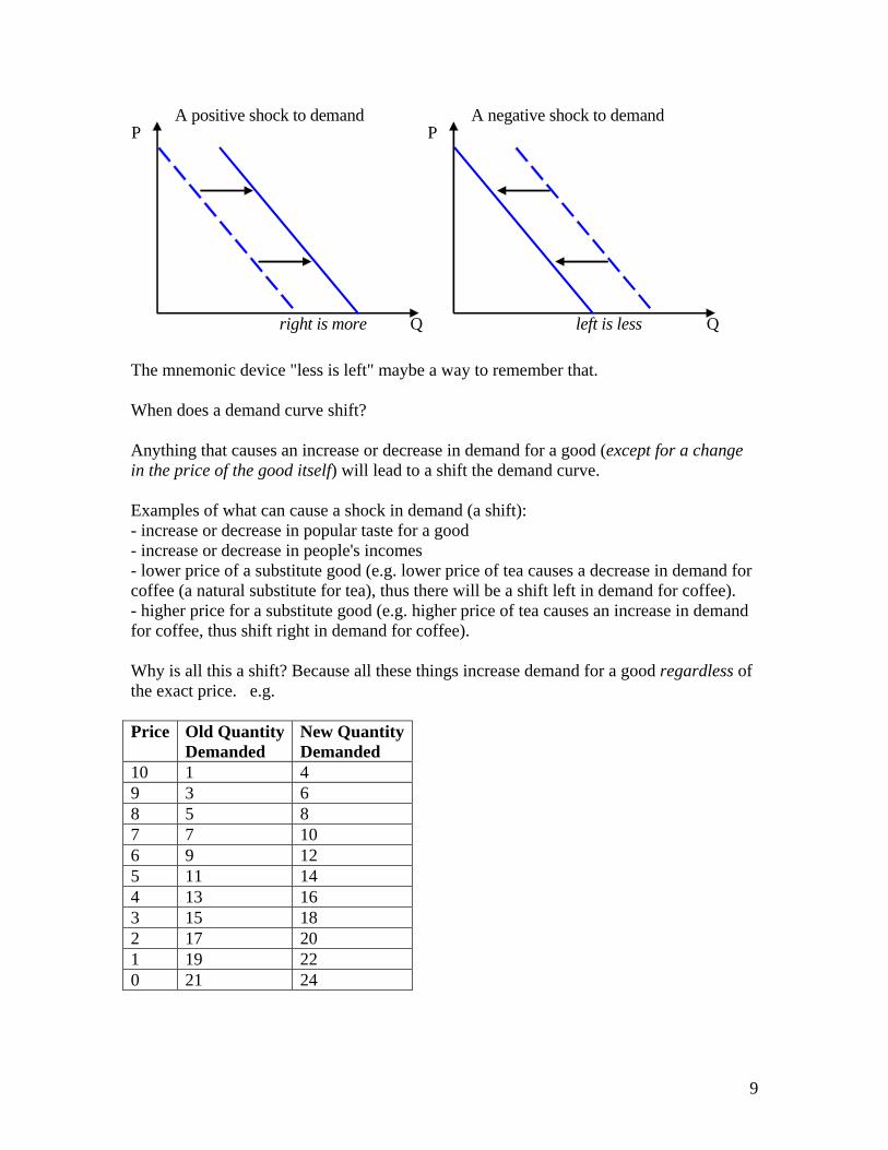
Notice that at every price, the quantity demanded is three units greater than it was before. These three extra units arise for any the reasons cited above - because people are suddenly richer, because there is a new fashionable taste for the good, etc. Plotted out it will look like:

1 2 3 4

5 6 7 8 9 10

1 2 3 4 5 6 7 8 9 10

x-axis

0 11

C

Q = -2P + 21

11 12 13

Quantity

Price

y-axis

• •

old intercept

B

• 12 13 14 15 16 17 18 19 20 21 22

• •

• •

• •

• •

Old Demand Curve

• •

• New Demand Curve

Q = -2P + 24 •

• •

• •

• •

• 23 24

new intercept

A change in the price of the good itself is traced by the shape of the demand curve, that is, it is a movement along the curve. e.g. in the diagram above, if coffee rises in price from $7 to $8, then demand for coffee goes down from 7 to 4 units. But since that change in demand is caused by a change in price (rather than income, taste, etc.), then that is represented as a movement along the curve from point B to point C. But anything else that affects demand (other than its own price) will be represented by a shift in the entire curve.

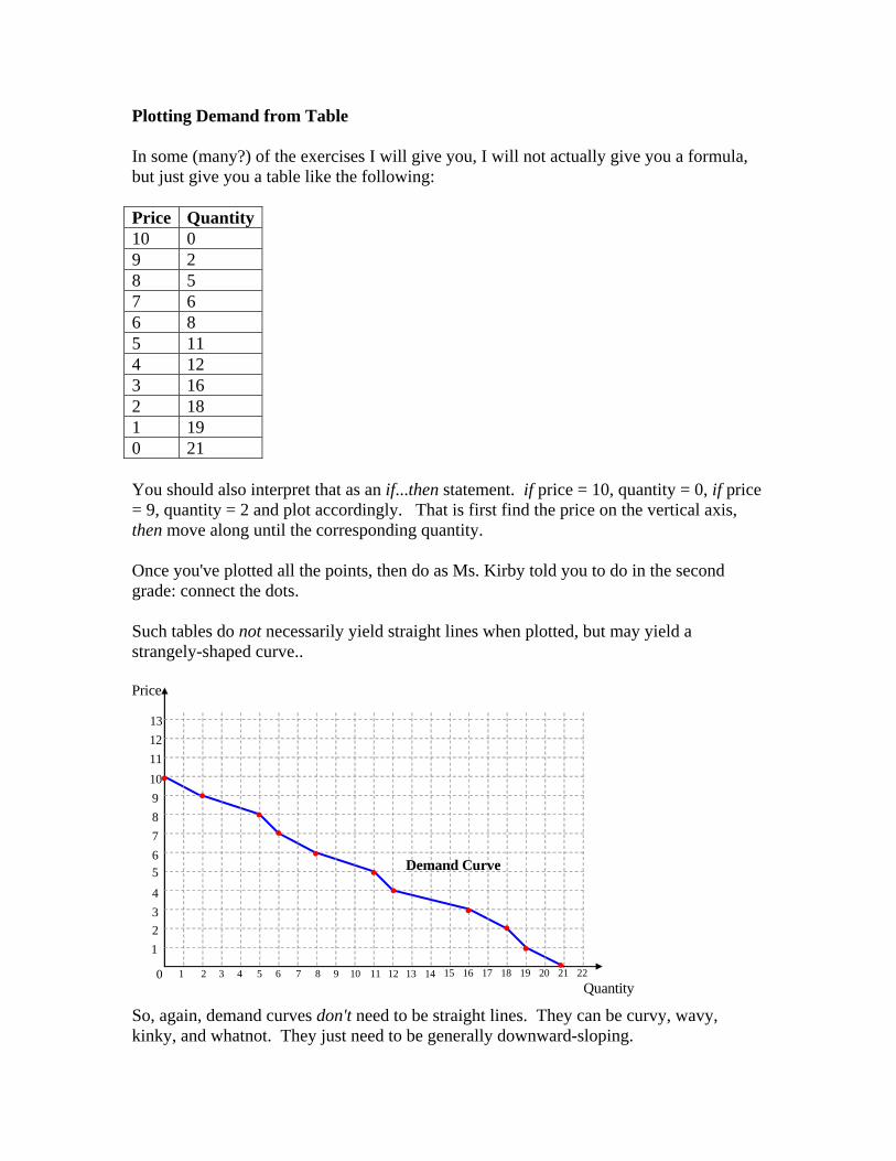
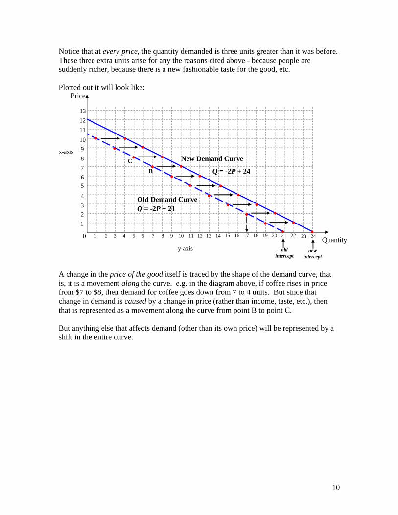
Plotting Demand from Table In some (many?) of the exercises I will give you, I will not actually give you a formula, but just give you a table like the following: Price Quantity 10 0 9 2 8 5 7 6 6 8 5 11 4 12 3 16 2 18 1 19 0 21 You should also interpret that as an if...then statement. if price = 10, quantity = 0, if price = 9, quantity = 2 and plot accordingly. That is first find the price on the vertical axis, then move along until the corresponding quantity. Once you've plotted all the points, then do as Ms. Kirby told you to do in the second grade: connect the dots. Such tables do not necessarily yield straight lines when plotted, but may yield a strangely-shaped curve..

1 2 3 4 5 6 7 8 9 10

1 2 3 4 5 6 7 8 9 10 0 11

11 12 13

Quantity

Price

• •

• 12 13 14 15 16 17 18 19 20 21 22

• •

• •

• •

• •

Demand Curve

So, again, demand curves don't need to be straight lines. They can be curvy, wavy, kinky, and whatnot. They just need to be generally downward-sloping.

12

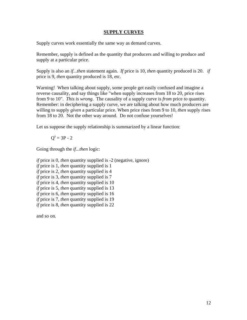
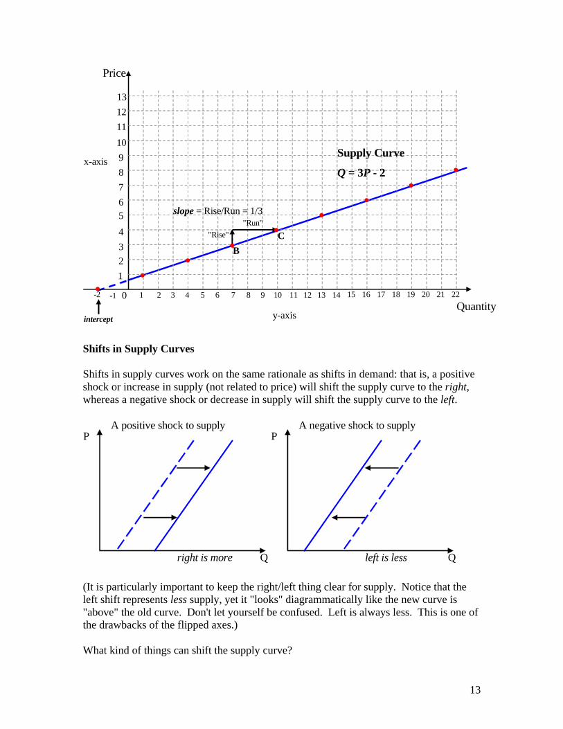
SUPPLY CURVES Supply curves work essentially the same way as demand curves. Remember, supply is defined as the quantity that producers and willing to produce and supply at a particular price. Supply is also an if...then statement again. If price is 10, then quantity produced is 20. if price is 9, then quantity produced is 18, etc. Warning! When talking about supply, some people get easily confused and imagine a reverse causality, and say things like "when supply increases from 18 to 20, price rises from 9 to 10". This is wrong. The causality of a supply curve is from price to quantity. Remember: in deciphering a supply curve, we are talking about how much producers are willing to supply given a particular price. When price rises from 9 to 10, then supply rises from 18 to 20. Not the other way around. Do not confuse yourselves! Let us suppose the supply relationship is summarized by a linear function: Qs = 3P - 2 Going through the if...then logic: if price is 0, then quantity supplied is -2 (negative, ignore) if price is 1, then quantity supplied is 1 if price is 2, then quantity supplied is 4 if price is 3, then quantity supplied is 7 if price is 4, then quantity supplied is 10 if price is 5, then quantity supplied is 13 if price is 6, then quantity supplied is 16 if price is 7, then quantity supplied is 19 if price is 8, then quantity supplied is 22 and so on.

13

1 2 3 4 5 6 7 8 9 10

1 2 3 4 5 6 7 8 9 10

x-axis

0 11

"Rise"

"Run"

C

Q = 3P - 2

11 12 13

Quantity

Price

y-axis

slope = Rise/Run = 1/3

intercept

B

• 12 13 14 15 16 17 18 19 20 21 22

• •

• •

• •

• •

Supply Curve

-2 -1

Shifts in Supply Curves Shifts in supply curves work on the same rationale as shifts in demand: that is, a positive shock or increase in supply (not related to price) will shift the supply curve to the right, whereas a negative shock or decrease in supply will shift the supply curve to the left.

Q

P A positive shock to supply

right is more

Q

P A negative shock to supply

left is less (It is particularly important to keep the right/left thing clear for supply. Notice that the left shift represents less supply, yet it "looks" diagrammatically like the new curve is "above" the old curve. Don't let yourself be confused. Left is always less. This is one of the drawbacks of the flipped axes.) What kind of things can shift the supply curve?

14

- bad weather that may destroy a crop (shift left) - a sudden increase in costs of production (workers' wages increase, higher energy costs) will reduce supply (shift left) - a sudden improvement in technology, particularly if it is cost saving, that allows more to be supplied without extra cost (shift right) and so on. Keep in mind that anything that affects the profitability of a firm (except for price itself) will be a shift in the curve. By contrast, a change in price affecting supply will be represented as a movement along the supply curve.

15

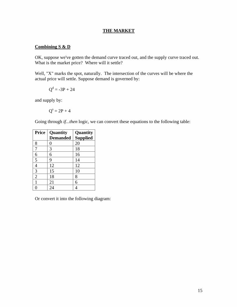
THE MARKET Combining S & D OK, suppose we've gotten the demand curve traced out, and the supply curve traced out. What is the market price? Where will it settle? Well, "X" marks the spot, naturally. The intersection of the curves will be where the actual price will settle. Suppose demand is governed by: Qd = -3P + 24 and supply by: Qs = 2P + 4 Going through if...then logic, we can convert these equations to the following table: Price Quantity

Demanded Quantity Supplied

8 0 20 7 3 18 6 6 16 5 9 14 4 12 12 3 15 10 2 18 8 1 21 6 0 24 4 Or convert it into the following diagram:

16

1 2 3 4

5 6 7 8 9 10

1 2 3 4 5 6 7 8 9 10 0 11

Qs = 2P + 4

11 12 13

Quantity

Price

• •

supply intercept

Excess Supply = 10

12 13 14 15 16 17 18 19 20 21 22

• •

• •

•

•

• •

Supply Curve

• •

•

Demand Curve

Qd = -3P + 24

•

•

• •

• 23 24

demand intercept

Excess Demand = 5

market-clearing equilibrium price

price too high

price too low

equilibrium quantity

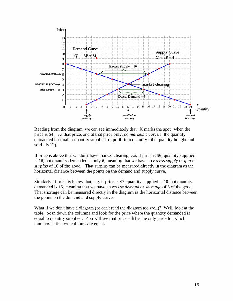
Reading from the diagram, we can see immediately that "X marks the spot" when the price is $4. At that price, and at that price only, do markets clear, i.e. the quantity demanded is equal to quantity supplied. (equilibrium quantity - the quantity bought and sold - is 12). If price is above that we don't have market-clearing, e.g. if price is $6, quantity supplied is 16, but quantity demanded is only 6, meaning that we have an excess supply or glut or surplus of 10 of the good. That surplus can be measured directly in the diagram as the horizontal distance between the points on the demand and supply curve. Similarly, if price is below that, e.g. if price is $3, quantity supplied is 10, but quantity demanded is 15, meaning that we have an excess demand or shortage of 5 of the good. That shortage can be measured directly in the diagram as the horizontal distance between the points on the demand and supply curve. What if we don't have a diagram (or can't read the diagram too well)? Well, look at the table. Scan down the columns and look for the price where the quantity demanded is equal to quantity supplied. You will see that price = $4 is the only price for which numbers in the two columns are equal.

17

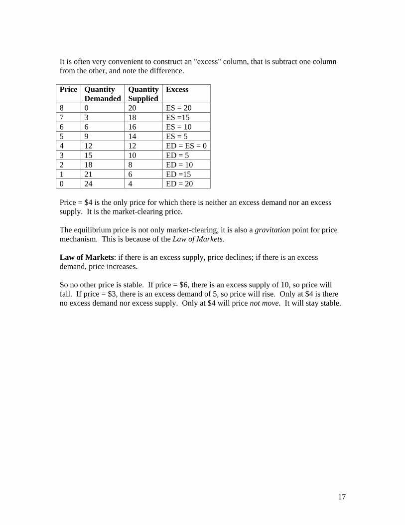
It is often very convenient to construct an "excess" column, that is subtract one column from the other, and note the difference. Price Quantity

Demanded Quantity Supplied

Excess

8 0 20 ES = 20 7 3 18 ES =15 6 6 16 ES = 10 5 9 14 ES = 5 4 12 12 ED = ES = 03 15 10 ED = 5 2 18 8 ED = 10 1 21 6 ED =15 0 24 4 ED = 20 Price = $4 is the only price for which there is neither an excess demand nor an excess supply. It is the market-clearing price. The equilibrium price is not only market-clearing, it is also a gravitation point for price mechanism. This is because of the Law of Markets. Law of Markets: if there is an excess supply, price declines; if there is an excess demand, price increases. So no other price is stable. If price = $6, there is an excess supply of 10, so price will fall. If price = $3, there is an excess demand of 5, so price will rise. Only at $4 is there no excess demand nor excess supply. Only at $4 will price not move. It will stay stable.

18

SOLVING EQUATIONS As we have seen, demand and supply curves are sometimes expressed as equations. If we have simple linear equations for demand and supply (which is nice, but not necessary), then we can easily solve for the equilibrium solution directly by using simple algebra, rather than going through the trouble of tracing diagrams or constructing tables. Algebra Rules There are really only a few rules of algebra to keep in mind (scratch your memory....) e.g. consider the equation: 3x + 5 = 0 x is called a variable the number multiplicatively attached to a variable (that is, 3) is called a coefficient. the number that is connected by summation or subtraction (that is 5) is called a constant. (i) Like combines with like. Constant terms can be added (subtracted if negative): e.g. in the equation 2x + 4 - 1 = 0, add constants 4 and -1 to yield 2x - 3 = 0. Coefficient terms are also combinable with other coefficient terms: e.g. in the equation 2x + 3x - 12 = 0, we can combine 2 and 3, so (2 + 3)x - 12 = 0, or simply 5x - 12 = 0 (but you can't combine coefficients with constants). (ii) if you move something from one side of the equal sign (=), to the other, then the sign of the term flips from positive to negative (or from negative to positive), e.g. if 3x - 2 = 5, then flipping -2 from the left to the right of the equal sign will yield 3x = 5 + 2. Notice that 2 changes sign from -2 to +2. e.g. if 2x = 9 + 4x, then flipping 4x from the right to the left side of the equal sign will yield 2x - 4x = 9, where notice 4x changes sign from +4x to -4x. (iii) The only way to get rid of coefficients is by dividing the whole expression.

19

e.g. suppose 5x = 20. 5 is a coefficient since it is multiplicatively attached to x, whereas 20 is a constant. Dividing the whole thing by 5 yields x = 20/5 or x = 5. Congratulations. You've solved for x. And that's all. Solving for Equilibrium Suppose demand is governed by: Qd = -3P + 24 and supply is governed by: Qs = 2P + 4 How do we find the equilibrium price without resorting to diagrams or tables? Algebra. We know that at the equilibrium price, the market will clear. That is, we know that at equilibrium, quantity demanded must equal quantity supplied, that is:

Qd = Qs This must be true (it is the definition of equilibrium). But what are Qd and Qs? You may say, "but that depends on price! It seems circular reasoning!" But it isn't. Just substitute the equations we have for Qd and Qs That is if Qd = Qs at equilibrium, then it must also be true that at equilibrium: -3P + 24 = 2P + 4 we've just plugged in our equations for for Qd and Qs. The P which solves this equation must be our equilibrium price. How do we solve? Well, first just use algebra. Let's flip the cofficients to one side, and the constants to the other side of the equal sign (keeping the flips in signs in mind): 24 - 4 = 2P + 3P combining like with like: 20 = (2 + 3)P or simply: 20 = 5P

20

Now we have a constant (20) and a coefficient (5). Dividing by 5, it must be that: P = 20/5 or simply: P = 4. That is, P = 4, is the price that clears the market. Is it? Well, we happened to use the equations we used before. We know $4 is the equilibrium price. Easy, wasn't it? OK, so we got the equilibrium price. How about the equilibrium quantity? That is even simpler. We know that the equilibrium quantity is the quantity demanded when the price is at equilibrium. Since we already found the equilibrium price is 4, then since Qd = -3P + 24, then equilibrium quantity must be: Q = -3 (4) + 24 or simply: Q = -12 + 24 or simply: Q = 12. And we're done. That's the equilibrium quantity. [Note: we also know the equilibrium quantity is the quantity supplied when the price is at equilibrium. So we could also use that equation instead. Since we know that P = 4 and Qs = 2P + 4, then equilibrium quantity: Q = 2(4) + 4 or Q = 8 + 4, or simply Q = 12. Same result. In practice, you don't have to repeat it. Just pick one or the other equation to solve for quantity.] So using algebra, we can deduce the equilibrium price and quantity rather quickly. Example #2 Let's try another example. Suppose the demand and supply functions are Qd = -6P + 140 Qs = 3P + 5

21

Let's do it again. Impose the equilibrium condition:

Qd = Qs then plug in our equations: -6P + 140 = 3P + 5 rearranging terms around: 140 - 5 = 3P + 6P or: 135 = 9P So solving for P: P = 135/9 = 15 Equilibrium price is $15. What about equilibrium quantity? Let's use the supply curve Qs = 3P + 5, so plugging in our equilibrium price (15) into it: Q = 3(15) + 5 or Q = 45 + 5 or simply: Q = 50 So equilibrium price is $15 and equilibrium quantity is 50 units. Example #3 One more? Suppose the demand and supply functions are Qd = -5P + 80 Qs = (7.5)P - 20 (yes, we can have fractions & decimals). Let's do it again. Set the equilibrium condition:

Qd = Qs plugging in our equations:

22

-5P + 80 = (7.5)P - 20 Combining: 80 + 20 = (7.5)P + 5P as 7.5 + 5 = 12.5, then: 100 = (12.5)P that means: P = 100/12.5 = $8. The equilibrium price is $8. To get equilibrium quantity, let's use the supply curve, Qs = 3P - 20: Q = (7.5)(8) - 20 or: Q = 60 - 20 so Q = 40. And we are done. Price is $8, quantity is 40. Non-linear Functions As mentioned, sometimes our demand and supply equations are not linear. Sometimes they are non-linear (curves, wavy, etc.). In principle, you should be able to solve them the same way. But since manipulating the expressions with exponents and stuff is a little more complicated, let's not bother. Rest assured I will (probably) be giving you any exercises using non-linear equations. (well, I will, but I'll ask you to solve by table or eyeballing diagrams). But just keep in mind that the same method can be used if you have the equations explicitly written out. Just impose the equilibrium condition (Qd = Qs), solve for P, then plug P in one equation and solve for Q.