Embed Size (px)
Citation preview
EEG/MEG Source Localization: Practical Application
Bioelectromagnetics and Neuroimaging Laboratory
Department of Biomedical Engineering, Yonsei University
Chang-Hwan Im, Ph.D.
http://bem.yonsei.ac.kr
http://bem.yonsei.ac.kr
Contents
1. Signal Processing
2. Pre-processing
3. Equivalent Current Dipole (ECD) Localization
4. EEG/MEG Source Imaging
5. Commercial/Open Software for EEG/MEG Source Imaging

http://bem.yonsei.ac.kr
Preparing Analysis
1. EEG/MEG Data (Raw data)
2. Structural MRI Data
3. Position of Electrodes or SQUID sensors
4. Anatomical Landmarks, Head Shape (optional)
http://bem.yonsei.ac.kr
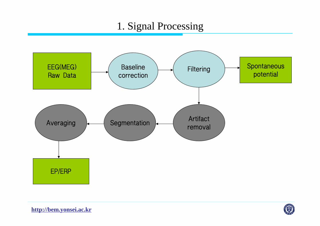
1. Signal Processing
EEG(MEG)Raw Data
Baselinecorrection
Filtering
SegmentationArtifactremoval
Averaging
EP/ERP
Spontaneouspotential
http://bem.yonsei.ac.kr
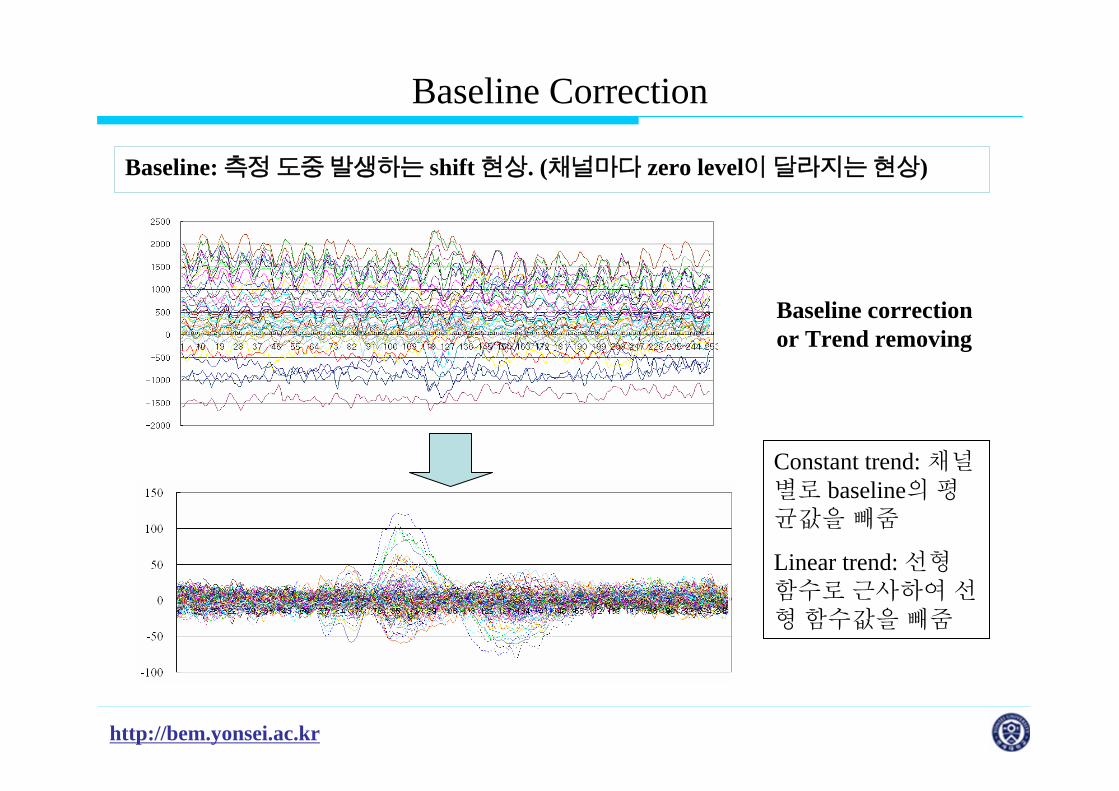
Baseline Correction
Baseline: 측정도중발생하는 shift 현상. (채널마다 zero level이달라지는현상)
Baseline correctionor Trend removing
Constant trend: 채널별로 baseline의 평균값을빼줌
Linear trend: 선형함수로근사하여선형함수값을빼줌

http://bem.yonsei.ac.kr
Filtering
Bandpass filtering(1 – 30 Hz)
일반적으로 band-pass filter 사용

http://bem.yonsei.ac.kr
Artifact Removal
왜발생하는가?
어떻게제거하는가?
ICA 등여러가지기술사용가능
http://bem.yonsei.ac.kr
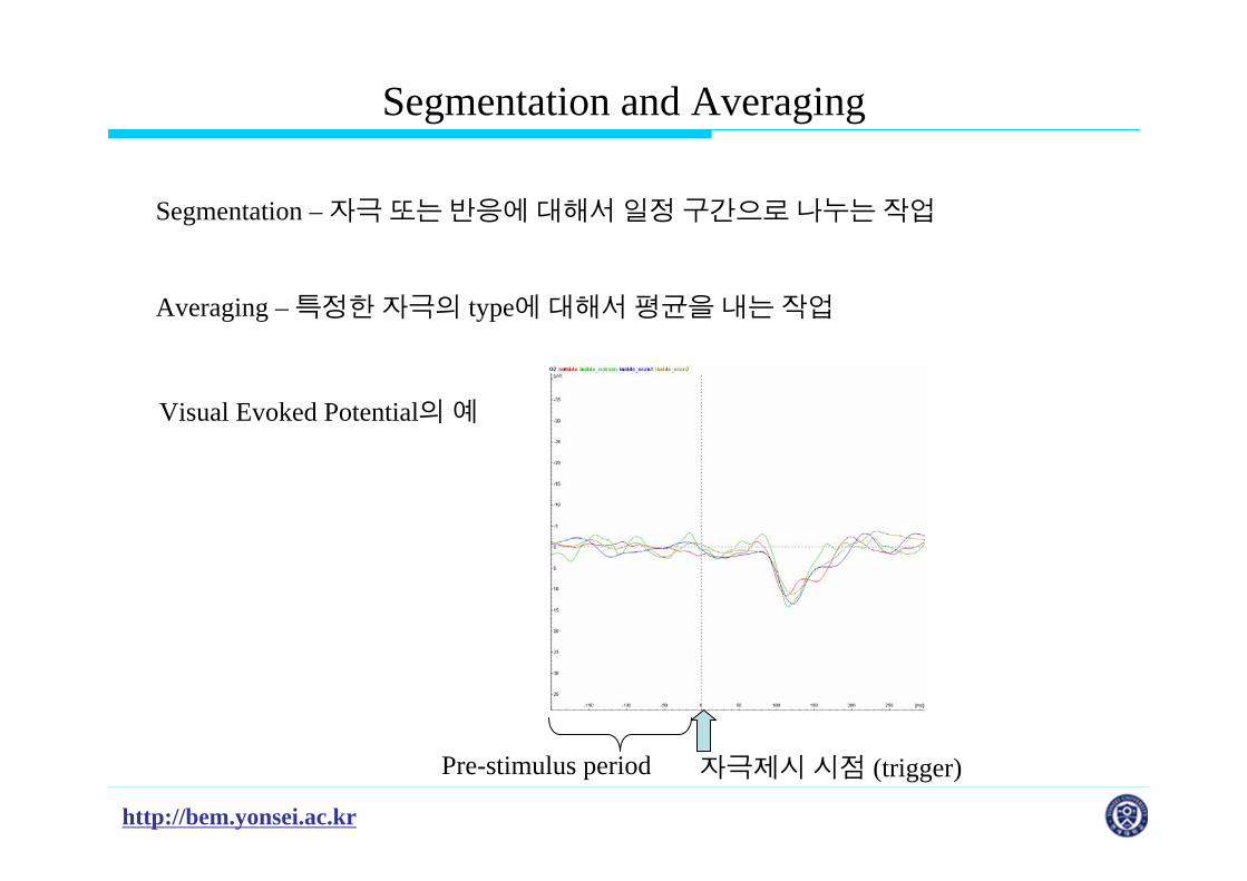
Segmentation and Averaging
Segmentation – 자극또는반응에대해서일정구간으로나누는작업
Averaging – 특정한자극의 type에대해서평균을내는작업
Visual Evoked Potential의예
자극제시시점 (trigger)Pre-stimulus period

http://bem.yonsei.ac.kr
참고 – Average Reference (EEG)
1
1ˆ ( ) ( )MN
i i ref j refjM
V V V V VN =
= − − −∑
Why reference is needed??
Where to put reference??
Average reference??

http://bem.yonsei.ac.kr
Contents
1. Signal Processing
2. Pre-processing
3. Equivalent Current Dipole (ECD) Localization
4. EEG/MEG Source Imaging
5. Commercial/Open Software for EEG/MEG Source Imaging
http://bem.yonsei.ac.kr
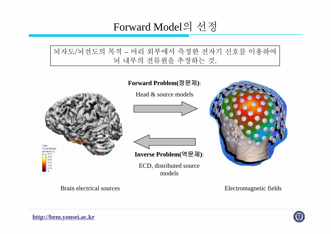
Forward Model의선정
Brain electrical sources Electromagnetic fields
Forward Problem(Forward Problem(정문제정문제)):
Head & source models
Inverse Problem(Inverse Problem(역문제역문제)):
ECD, distributed source models
뇌자도/뇌전도의 목적 – 머리 외부에서 측정한 전자기 신호를 이용하여뇌 내부의 전류원을 추정하는 것.
http://bem.yonsei.ac.kr
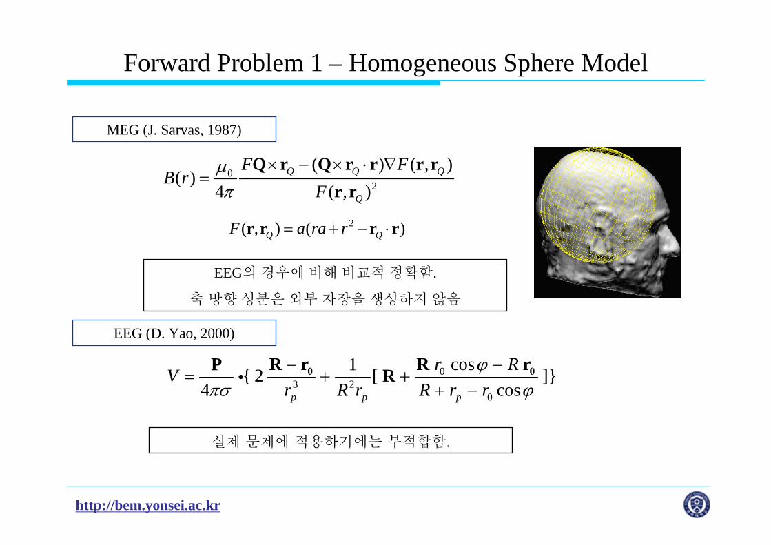
Forward Problem 1 – Homogeneous Sphere Model
MEG (J. Sarvas, 1987)
EEG (D. Yao, 2000)
03 2
0
cos1{ 2 [ ]}4 cosp p p
r RVr R r R r r
ϕπσ ϕ
− −= + +
+ −0 0R r R rP Ri
EEG의경우에비해 비교적 정확함.
축 방향성분은외부 자장을 생성하지않음
실제 문제에 적용하기에는 부적합함.
02
( ) ( , )( )
4 ( , )Q Q Q
Q
F FB r
Fμπ
× − × ⋅ ∇=
Q r Q r r r rr r
2( , ) ( )Q QF a ra r= + − ⋅r r r r

http://bem.yonsei.ac.kr
Forward Problem 2 – Concentric Sphere Model
brain
Inner skull
Outer skull
scalp
• EEG의 경우에는 정해(exact solution) 존재, MEG의경우에는근사해만존재.
• MEG의 경우에는 거의 사용 안 함 . MEG의 경우에는 두개골(skull) 밖으로나가는 전류가 대부분 차단되기 때문에단일 구형 도체 모델을 사용하는 경우와정확도차이가거의없음.
• EEG의 경우에는 정확도가 많이 향상됨. 하지만 실제 뇌의 구조를 고려하는경우와는 정확도 차이가 많이 남. 특수한영역에서만정확도보장
실제 문제에서는 보다 정확한 모델이필요하다.
Head fitting

http://bem.yonsei.ac.kr
Forward Problem 3 – 경계요소법
0 0( ) ( ) 2 ( )
1 '( ) ( ') ( ') ,2 ij
i j
i j Sij
V V
V d
σ σ σ
σ σπ
+ =
+ − Ω∑ ∫ r
r r
r r ∫⋅∇
=G
p
dvR
V ')'('4
1)(0
0rJr
πσ
∑ ∫ ×−+=ij
S ijjiij RV 'dSRrrBrB 3
00 )'()(
4)()( σσ
πμ
∫ ×= ')'(4
)( 30
0 dvR
pG
RrJrBπμ
In EEG
In MEG, after solving EEG problem
일반적으로 3~4층의다른전기전도도를지니는영역으로분류
하고각영역은균일하고isotropic conductivity를가진다
고가정함.
뇌자도는일반적으로두개골안쪽경계부분만사용
http://bem.yonsei.ac.kr
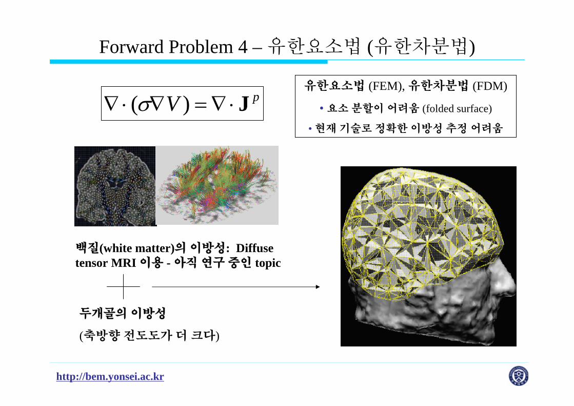
Forward Problem 4 – 유한요소법 (유한차분법)
백질(white matter)의 이방성: Diffuse tensor MRI 이용 - 아직 연구 중인 topic
두개골의 이방성
(축방향 전도도가 더 크다)
유한요소법 (FEM), 유한차분법 (FDM)
• 요소 분할이 어려움 (folded surface)
• 현재 기술로 정확한 이방성 추정 어려움
pV J⋅∇=∇⋅∇ )(σ

http://bem.yonsei.ac.kr
When anatomical information is not available
1. Use of standard head model/sensor configuration: MNI model is usually used.- CURRY, BESA, BrainStorm 등에서모두지원하며 LORETA는 standard만지원함
2. Scalp surface를이용한 BEM model의생성
http://bem.yonsei.ac.kr
Pre-processing for EEG/MEG Analysis
Boundary Element Method와 Distributed Source Model을 사용한다고 가정하였을 때의 Pre-processing 과정
http://bem.yonsei.ac.kr
Preprocessing for MEG Analysis
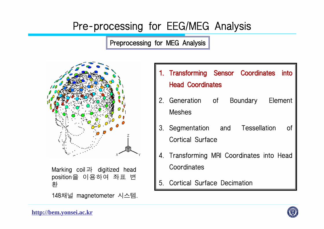
1.1. Transforming Sensor Coordinates into Transforming Sensor Coordinates into
Head Coordinates Head Coordinates
2. Generation of Boundary Element
Meshes
3. Segmentation and Tessellation of
Cortical Surface
4. Transforming MRI Coordinates into Head
Coordinates
5. Cortical Surface Decimation
Marking coil과 digitized head position을 이용하여 좌표 변환
148채널 magnetometer 시스템.
Pre-processing for EEG/MEG Analysis

http://bem.yonsei.ac.kr
Preprocessing for MEG Analysis
1. Transforming Sensor Coordinates into
Head Coordinates
2.2. Generation of Boundary Element Meshes Generation of Boundary Element Meshes
3. Segmentation and Tessellation of
Cortical Surface
4. Transforming MRI Coordinates into Head
Coordinates
5. Cortical Surface Decimation Inner skull boundary만을 삼각형 요소를 이용하여 분할.
Pre-processing for EEG/MEG Analysis
http://bem.yonsei.ac.kr
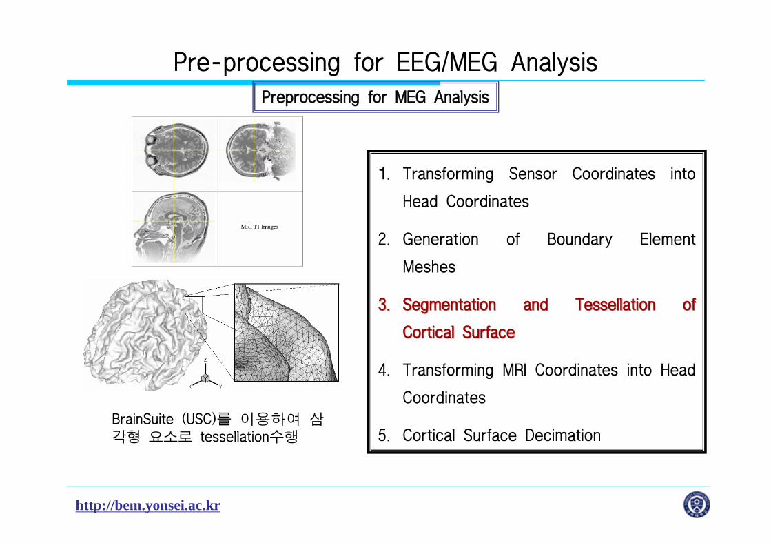
Preprocessing for MEG Analysis
1. Transforming Sensor Coordinates into
Head Coordinates
2. Generation of Boundary Element
Meshes
3.3. Segmentation and Tessellation of Segmentation and Tessellation of
Cortical SurfaceCortical Surface
4. Transforming MRI Coordinates into Head
Coordinates
5. Cortical Surface Decimation BrainSuite (USC)를 이용하여 삼각형 요소로 tessellation수행
Pre-processing for EEG/MEG Analysis

http://bem.yonsei.ac.kr
Preprocessing for MEG Analysis
1. Transforming Sensor Coordinates into
Head Coordinates
2. Generation of Boundary Element
Meshes
3. Segmentation and Tessellation of
Cortical Surface
4.4. Transforming MRI Coordinates into Head Transforming MRI Coordinates into Head
CoordinatesCoordinates
5. Cortical Surface Decimation Tessellated scalp surface 와digitized head position을 맞춤으로써 좌표 변환.
Pre-processing for EEG/MEG Analysis
http://bem.yonsei.ac.kr
Preprocessing for MEG Analysis
1. Transforming Sensor Coordinates into
Head Coordinates
2. Generation of Boundary Element
Meshes
3. Segmentation and Tessellation of
Cortical Surface
4. Transforming MRI Coordinates into Head
Coordinates
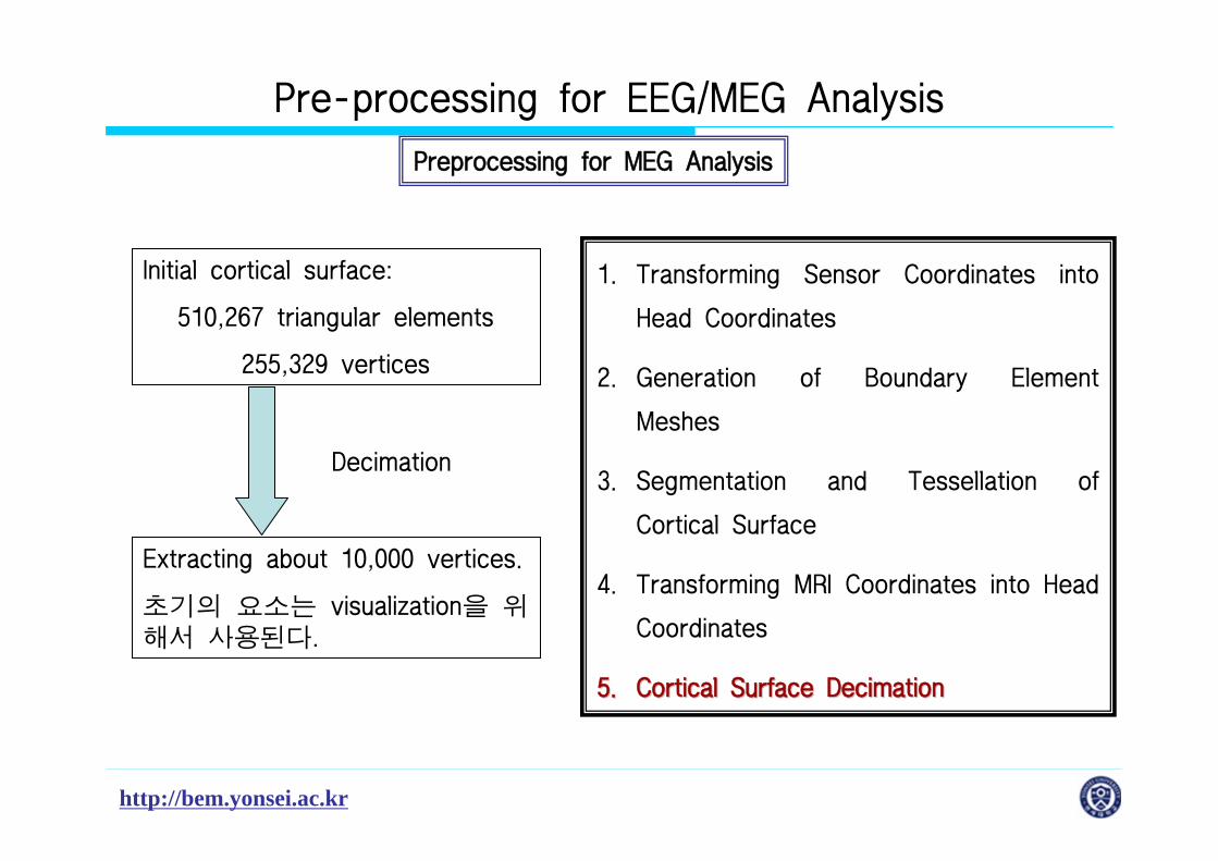
5.5. Cortical Surface Decimation Cortical Surface Decimation
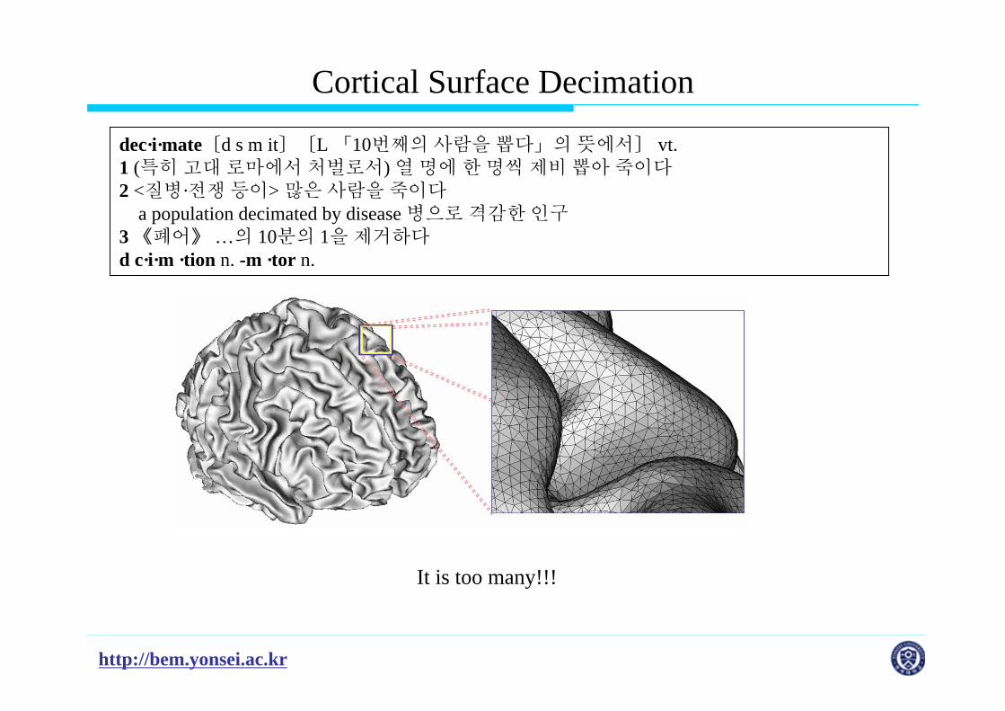
Initial cortical surface:
510,267 triangular elements
255,329 vertices
Decimation
Extracting about 10,000 vertices.
초기의 요소는 visualization을 위해서 사용된다.
Pre-processing for EEG/MEG Analysis
http://bem.yonsei.ac.kr
Cortical Surface Decimation
dec·i·mate〔d s m it〕〔L 「10번째의사람을뽑다」의 뜻에서〕 vt.1 (특히고대 로마에서처벌로서) 열 명에 한명씩 제비뽑아 죽이다2 <질병·전쟁 등이> 많은사람을죽이다
a population decimated by disease 병으로격감한인구3 《폐어》 …의 10분의 1을 제거하다d c·i·m ·tion n. -m ·tor n.
It is too many!!!
http://bem.yonsei.ac.kr
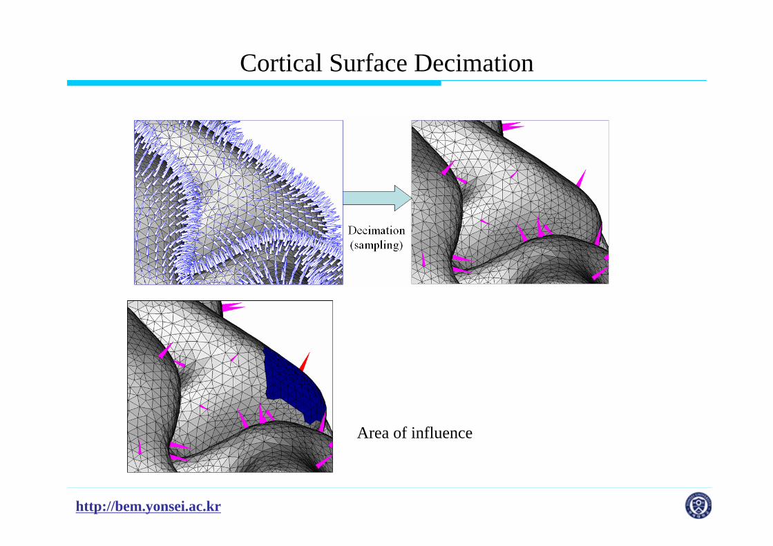
Cortical Surface Decimation
Area of influence

http://bem.yonsei.ac.kr
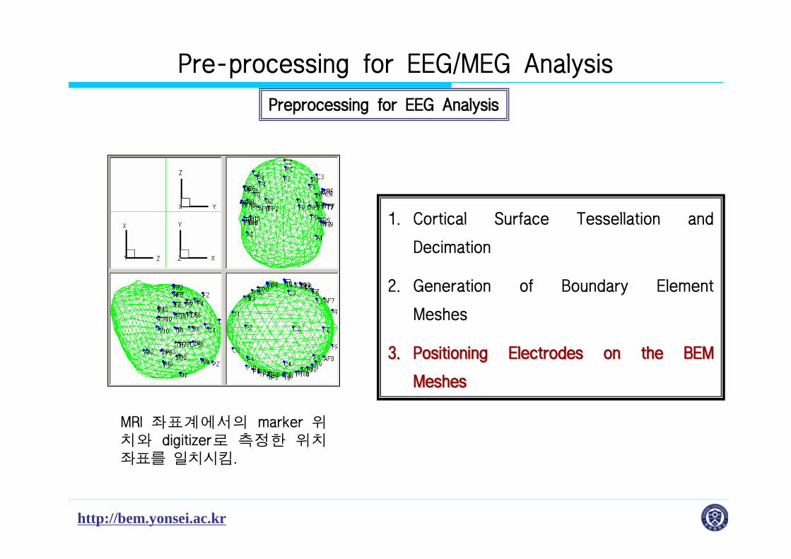
Preprocessing for EEG Analysis
1.1. Cortical Surface Tessellation and Cortical Surface Tessellation and
DecimationDecimation
2. Generation of Boundary Element
Meshes
3. Positioning Electrodes on the BEM
Meshes
Extract about 10,000 vertices from 641,195 elements and 321,698 vertices using decimation process.
Pre-processing for EEG/MEG Analysis

http://bem.yonsei.ac.kr
Preprocessing for EEG Analysis
1. Cortical Surface Tessellation and
Decimation
2.2. Generation of Boundary Element MeshesGeneration of Boundary Element Meshes
3. Positioning Electrodes on the BEM
Meshes
3260 elements and 1836 vertices
Pre-processing for EEG/MEG Analysis
http://bem.yonsei.ac.kr
Preprocessing for EEG Analysis
1. Cortical Surface Tessellation and
Decimation
2. Generation of Boundary Element
Meshes
3.3. Positioning Electrodes on the BEM Positioning Electrodes on the BEM
MeshesMeshes
MRI 좌표계에서의 marker 위치와 digitizer로 측정한 위치좌표를 일치시킴.
Pre-processing for EEG/MEG Analysis
http://bem.yonsei.ac.kr
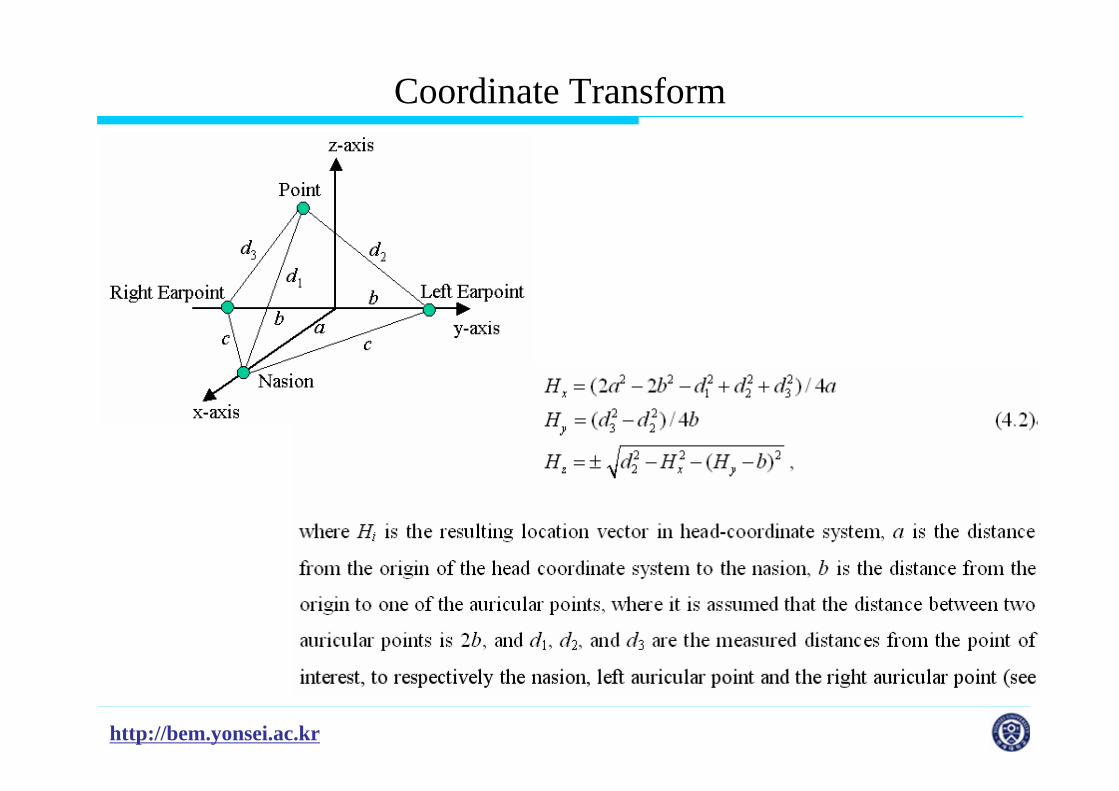
Coordinate Transform

http://bem.yonsei.ac.kr
Constructing Leadfield Matrix
x = As + n
Orientation Constraint가있을경우: Size of A - #sensors by #variables
구하는방법
Orientation Constraint가없을경우: Size of A – #sensors by #variables*3
구하는방법

http://bem.yonsei.ac.kr
Contents
1. Signal Processing
2. Pre-processing
3. Equivalent Current Dipole (ECD) Localization
4. EEG/MEG Source Imaging
5. Commercial/Open Software for EEG/MEG Source Imaging
http://bem.yonsei.ac.kr
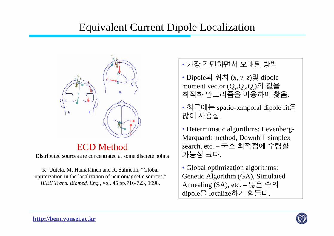
Equivalent Current Dipole Localization
ECD MethodDistributed sources are concentrated at some discrete points
K. Uutela, M. Hämäläinen and R. Salmelin, “Global optimization in the localization of neuromagnetic sources,”
IEEE Trans. Biomed. Eng., vol. 45 pp.716-723, 1998.
• 가장간단하면서오래된방법
• Dipole의위치 (x, y, z)및 dipole moment vector (Qx,Qy,Qz)의값을최적화알고리즘을이용하여찾음.
• 최근에는 spatio-temporal dipole fit을많이사용함.
• Deterministic algorithms: Levenberg-Marquardt method, Downhill simplex search, etc. – 국소최적점에수렴할가능성크다.
• Global optimization algorithms: Genetic Algorithm (GA), Simulated Annealing (SA), etc. – 많은수의dipole을 localize하기 힘들다.

http://bem.yonsei.ac.kr
Equivalent Current Dipole Localization (Cont’d)
Instantaneous Dipole Fit vs Spatio-temporal Dipole Fit
Spatio-temporal Dipole Fit이 Noise 성분에대해보다 robust하다 (대부분사용).
2|| ( ) ||FE = −x A p sError Function
where x is the measured electromagnetic signals, A lead field matrix that relates sensor positions and source locations, p location parameters of dipoles, and s corresponding dipole moment vectors.

http://bem.yonsei.ac.kr
Spatio-temporal Dipole Fit
Definition of Frobenius norm: 2|| ||F ija= ∑A
, where aij is i-th row and j-th column of the matrix A.
2|| ( ) ||FE = −x A p s
Spatio-temporal dipole fit utilizes series of multiple time samples.
Classification of ECDs:
(1) Moving dipole: 6 DOF – location vector (3 components) + moment vector (3 components)
(2) Rotating dipole: 3 DOF – location vector (3 components)
(3) Fixed dipole: do not need any nonlinear optimization
http://bem.yonsei.ac.kr
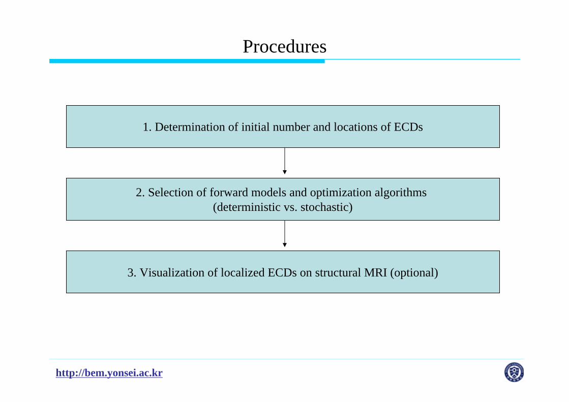
Procedures
1. Determination of initial number and locations of ECDs
2. Selection of forward models and optimization algorithms (deterministic vs. stochastic)
3. Visualization of localized ECDs on structural MRI (optional)
http://bem.yonsei.ac.kr
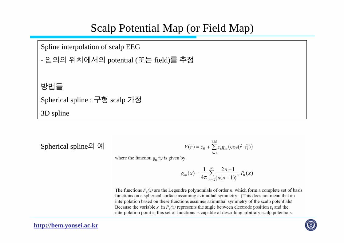
Scalp Potential Map (or Field Map)Spline interpolation of scalp EEG
- 임의의위치에서의 potential (또는 field)를추정
방법들
Spherical spline : 구형 scalp 가정
3D spline
Spherical spline의예
http://bem.yonsei.ac.kr
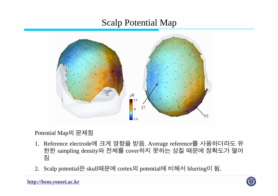
Scalp Potential Map
Potential Map의문제점
1. Reference electrode에 크게 영향을 받음. Average reference를 사용하더라도 유한한 sampling density와 전체를 cover하지 못하는 성질 때문에 정확도가 떨어짐
2. Scalp potential은 skull때문에 cortex의 potential에 비해서 blurring이됨.
http://bem.yonsei.ac.kr
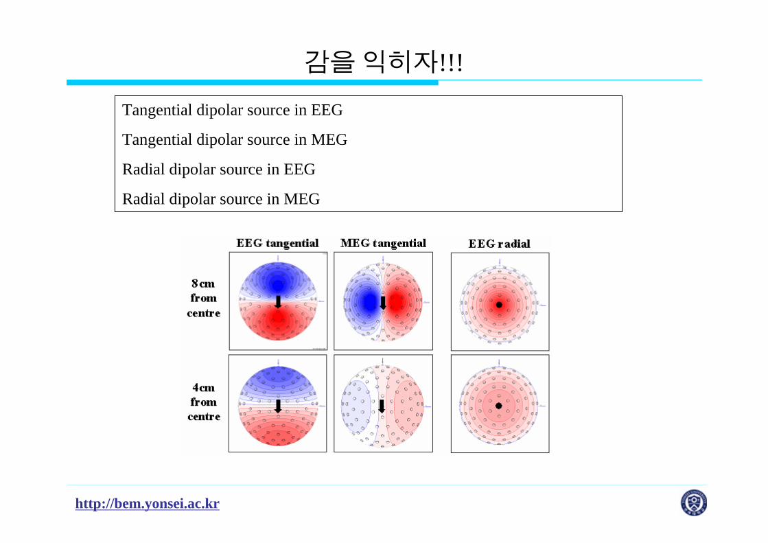
감을익히자!!!
Tangential dipolar source in EEG
Tangential dipolar source in MEG
Radial dipolar source in EEG
Radial dipolar source in MEG
http://bem.yonsei.ac.kr Bioelectromagnetics and Neuroimaging Lab.Bioelectromagnetics and Neuroimaging Lab. Yonsei BME
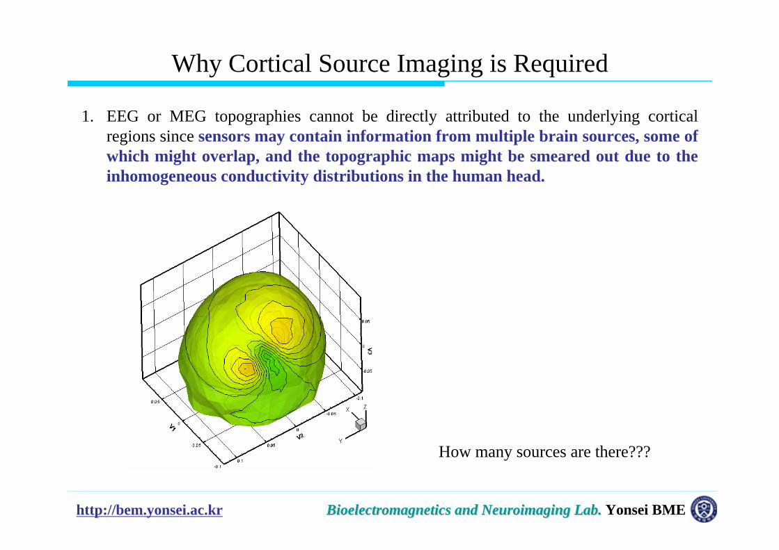
Why Cortical Source Imaging is Required
1. EEG or MEG topographies cannot be directly attributed to the underlying cortical regions since sensors may contain information from multiple brain sources, some of which might overlap, and the topographic maps might be smeared out due to the inhomogeneous conductivity distributions in the human head.
How many sources are there???
http://bem.yonsei.ac.kr Bioelectromagnetics and Neuroimaging Lab.Bioelectromagnetics and Neuroimaging Lab. Yonsei BME
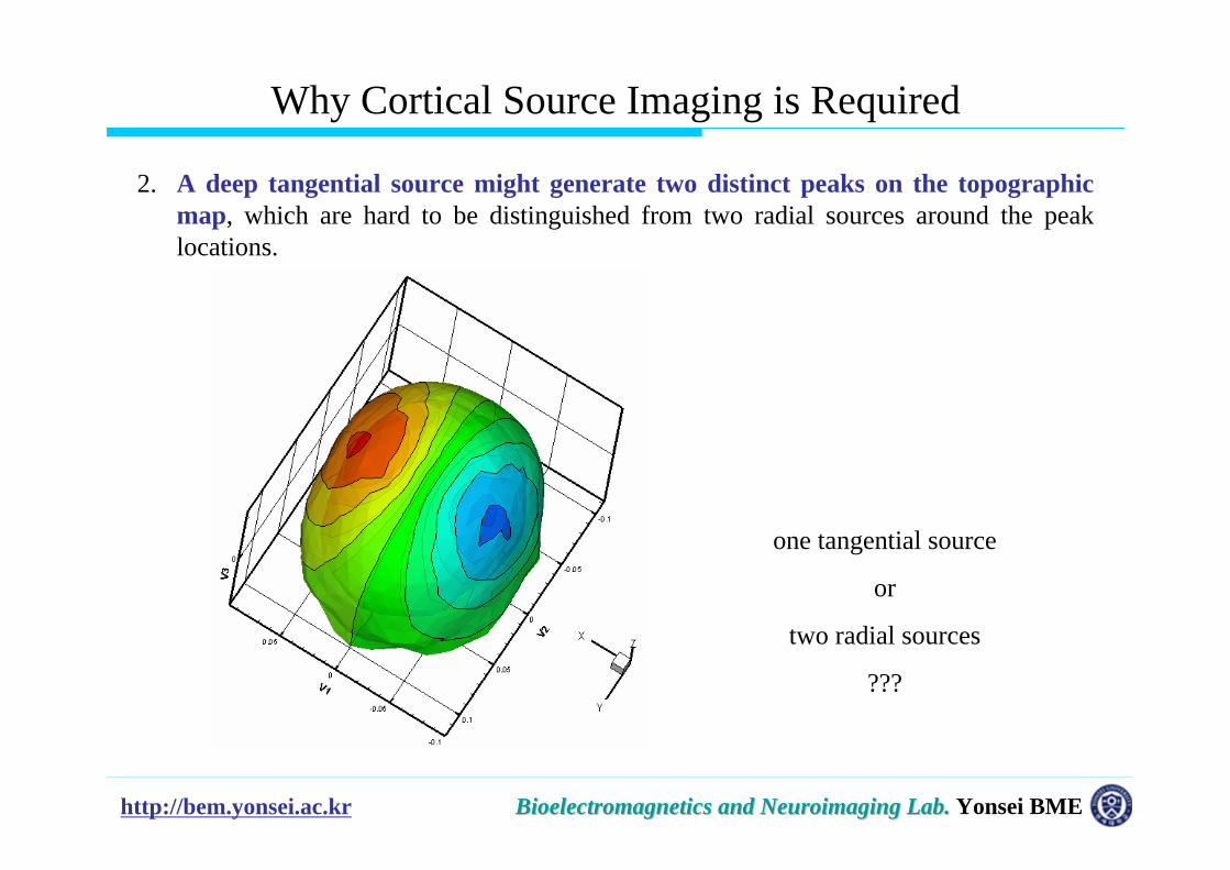
2. A deep tangential source might generate two distinct peaks on the topographic map, which are hard to be distinguished from two radial sources around the peak locations.
one tangential source
or
two radial sources
???
Why Cortical Source Imaging is Required
http://bem.yonsei.ac.kr Bioelectromagnetics and Neuroimaging Lab.Bioelectromagnetics and Neuroimaging Lab. Yonsei BME
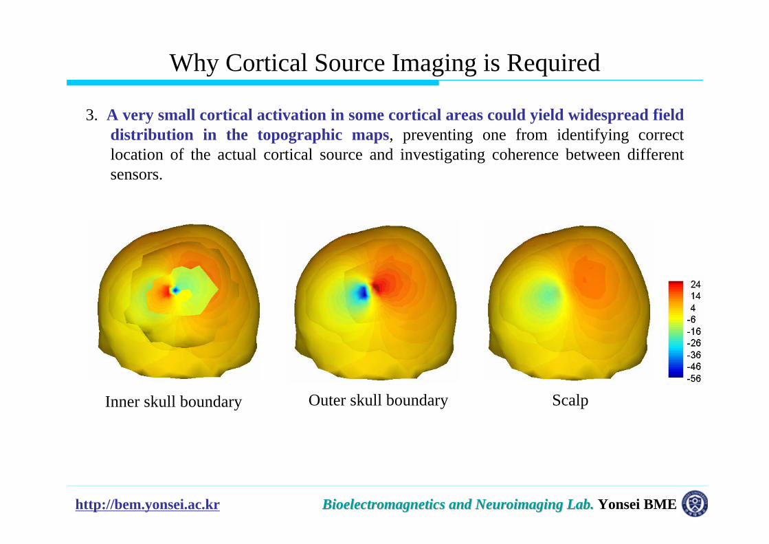
3. A very small cortical activation in some cortical areas could yield widespread field distribution in the topographic maps, preventing one from identifying correct location of the actual cortical source and investigating coherence between different sensors.
Inner skull boundary Outer skull boundary Scalp
Why Cortical Source Imaging is Required
http://bem.yonsei.ac.kr Bioelectromagnetics and Neuroimaging Lab.Bioelectromagnetics and Neuroimaging Lab. Yonsei BME
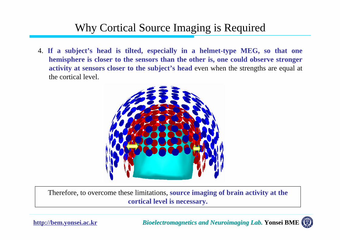
4. If a subject’s head is tilted, especially in a helmet-type MEG, so that one hemisphere is closer to the sensors than the other is, one could observe stronger activity at sensors closer to the subject’s head even when the strengths are equal at the cortical level.
Therefore, to overcome these limitations, source imaging of brain activity at the cortical level is necessary.
Why Cortical Source Imaging is Required

http://bem.yonsei.ac.kr
How to Estimate the Number of ECDs
1. Goodness of Fit (GOF)Goodness of Fit이 saturate되는 지점의 number of source 이용Goodness of Fit의정의: the squared sum of the signal explained by the model divided by the squared sum of the total signal
2. Independent Component Analysis (ICA)
3. MUSIC or FINE Algorithm
4. fMRI constraint

http://bem.yonsei.ac.kr
Use of ICA: Example 1
http://bem.yonsei.ac.kr
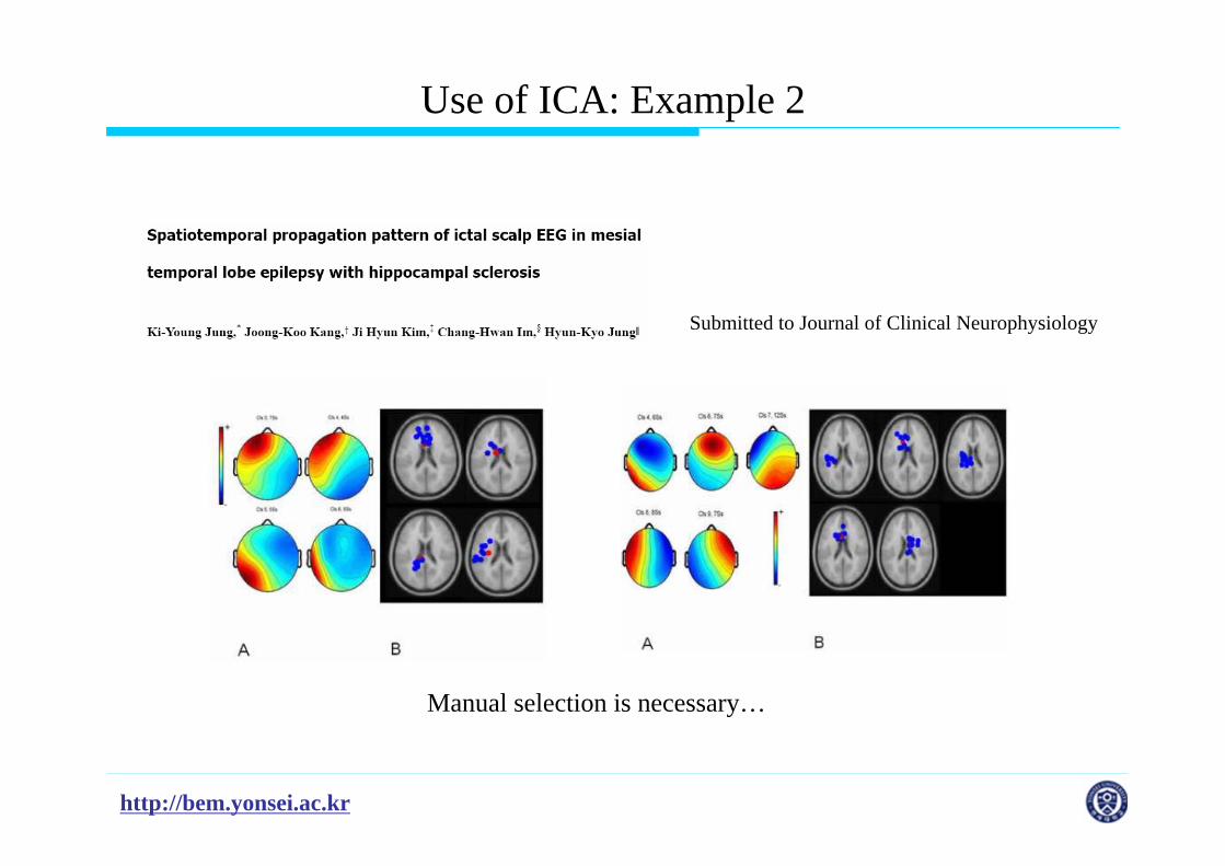
Use of ICA: Example 2
Submitted to Journal of Clinical Neurophysiology
Manual selection is necessary…
http://bem.yonsei.ac.kr
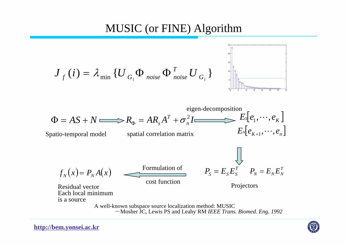
MUSIC (or FINE) Algorithm
}{)( min ii GTnoisenoiseGf UUiJ ΦΦ= λ
NAS +=Φ IAARR nT
s2σ+=Φ
spatial correlation matrix
eigen-decomposition
TSSS EEP = T
NNN EEP =
Projectors
( ) ( )xAPxf NN =Formulation of
cost functionResidual vectorEach local minimum is a source
[ ]nK eeEN ,,1+Spatio-temporal model
[ ]Ks eeE ,,1
A well-known subspace source localization method: MUSIC―Mosher JC, Lewis PS and Leahy RM IEEE Trans. Biomed. Eng. 1992

http://bem.yonsei.ac.kr
An Example
Potential problems
1. Solutions are dependent on the number of signal subspaces.
2. Cannot separate temporally correlated sources
http://bem.yonsei.ac.kr
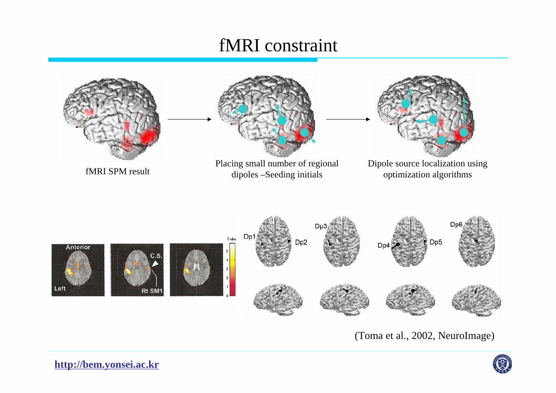
fMRI constraint
fMRI SPM resultPlacing small number of regional
dipoles –Seeding initialsDipole source localization using
optimization algorithms
(Toma et al., 2002, NeuroImage)
http://bem.yonsei.ac.kr
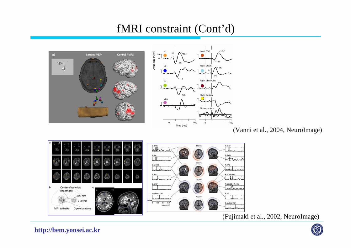
fMRI constraint (Cont’d)
(Vanni et al., 2004, NeuroImage)
(Fujimaki et al., 2002, NeuroImage)
http://bem.yonsei.ac.kr
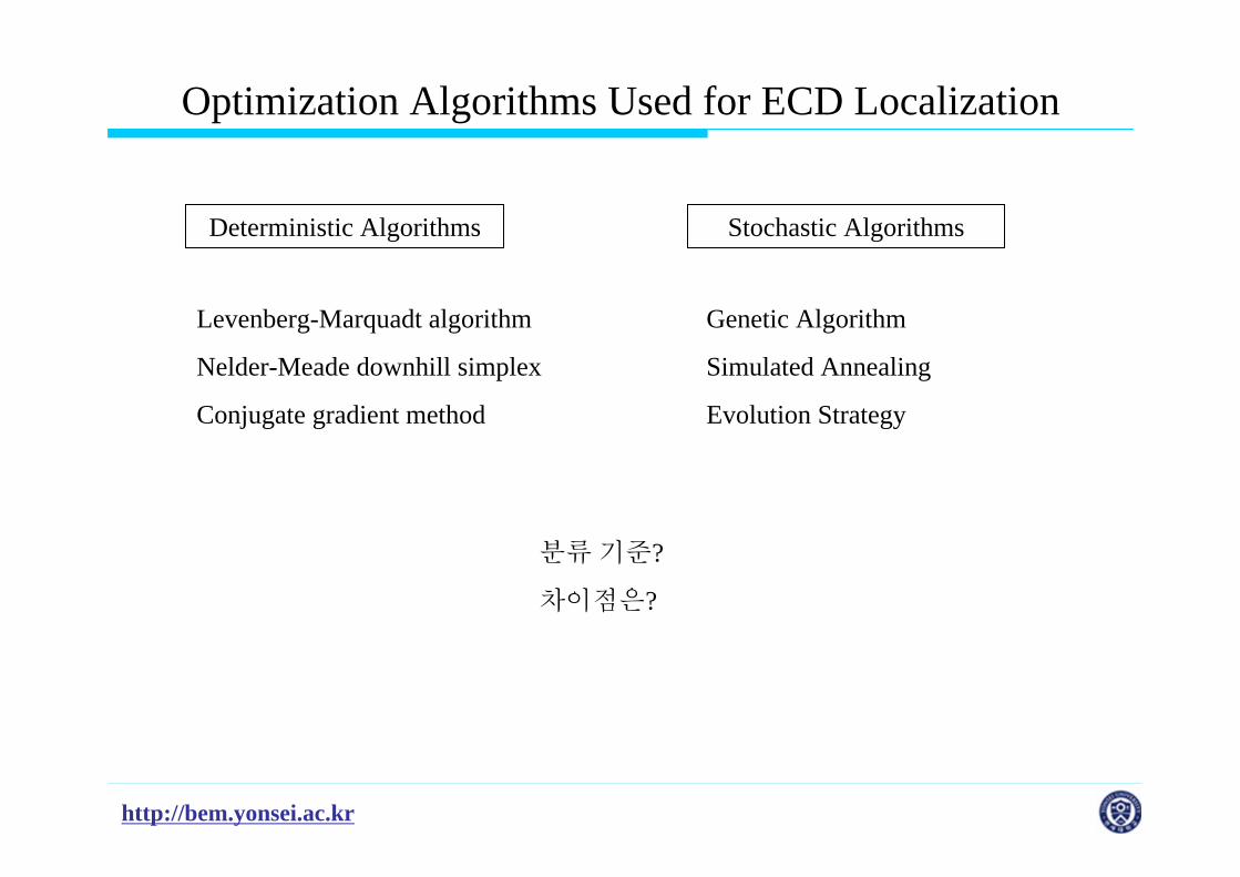
Optimization Algorithms Used for ECD Localization
Deterministic Algorithms Stochastic Algorithms
Levenberg-Marquadt algorithm
Nelder-Meade downhill simplex
Conjugate gradient method
Genetic Algorithm
Simulated Annealing
Evolution Strategy
분류기준?
차이점은?

http://bem.yonsei.ac.kr
Contents
1. Signal Processing
2. Pre-processing
3. Equivalent Current Dipole (ECD) Localization
4. EEG/MEG Source Imaging
5. Commercial/Open Software for EEG/MEG Source Imaging
http://bem.yonsei.ac.kr
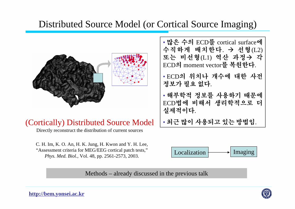
(Cortically) Distributed Source ModelDirectly reconstruct the distribution of current sources
C. H. Im, K. O. An, H. K. Jung, H. Kwon and Y. H. Lee, “Assessment criteria for MEG/EEG cortical patch tests,”
Phys. Med. Biol., Vol. 48, pp. 2561-2573, 2003.
• 많은 수의 ECD를 cortical surface에수직하게 배치한다 . 선형(L2) 또는 비선형(L1) 역산 과정 각ECD의 moment vector를 복원한다.
• ECD의 위치나 개수에 대한 사전정보가 필요 없다.
• 해부학적 정보를 사용하기 때문에ECD법에 비해서 생리학적으로 더실제적이다.
• 최근 많이 사용되고 있는 방법임.
Distributed Source Model (or Cortical Source Imaging)
Localization Imaging
Methods – already discussed in the previous talk
http://bem.yonsei.ac.kr
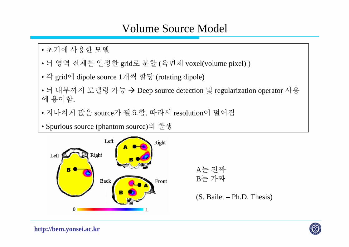
Volume Source Model
• 초기에사용한모델
• 뇌영역전체를일정한 grid로분할 (육면체 voxel(volume pixel) )
• 각 grid에 dipole source 1개씩할당 (rotating dipole)
• 뇌내부까지모델링가능 Deep source detection 및 regularization operator 사용에용이함.
• 지나치게많은 source가필요함. 따라서 resolution이떨어짐
• Spurious source (phantom source)의 발생
A는진짜B는가짜
(S. Bailet – Ph.D. Thesis)
http://bem.yonsei.ac.kr
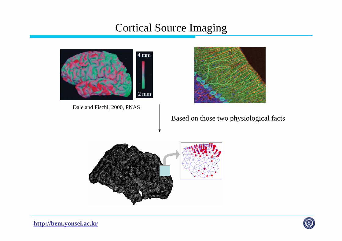
Cortical Source Imaging
Based on those two physiological factsDale and Fischl, 2000, PNAS

http://bem.yonsei.ac.kr
Orientation Constraint
1. Cortical surface가잘생성되었을경우 orientation constraint를 부여하는것이좋음
2. Cortical surface가잘생성되지않았을경우 orientation constraint를부여하면정확한결과를얻을수없음
http://bem.yonsei.ac.kr
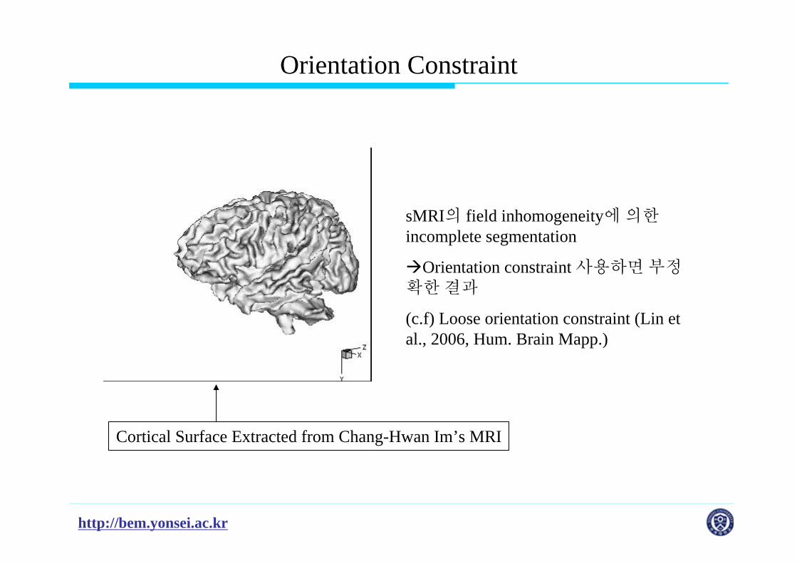
Orientation Constraint
sMRI의 field inhomogeneity에 의한incomplete segmentation
Orientation constraint 사용하면부정확한결과
(c.f) Loose orientation constraint (Lin et al., 2006, Hum. Brain Mapp.)
Cortical Surface Extracted from Chang-Hwan Im’s MRI
http://bem.yonsei.ac.kr
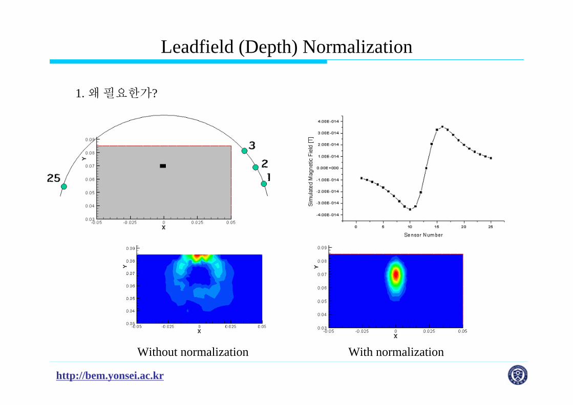
Leadfield (Depth) Normalization
1. 왜필요한가?
Without normalization With normalization

http://bem.yonsei.ac.kr
Leadfield (Depth) Normalization
2. Implementation
k-th dipole 성분에다음 term을곱해줌.
일반적인 p값은 ½를사용해왔음.
p = 0.75 가적합함을최근에밝힘 (Lin et al., 2006, Neuroimage)

http://bem.yonsei.ac.kr
Source Imaging에서 Pre-processing과 processing은분리가능!!
Forward model
Coordinate transform
Pre-processing
Generation of
Leadfield
Matrix A
Using Only
Geometry
Information
W = RAT (ARAT + λ2 C)-1
Linear inverse operator
sx = Ws
You can obtain A usingBrainStorm!
http://bem.yonsei.ac.kr
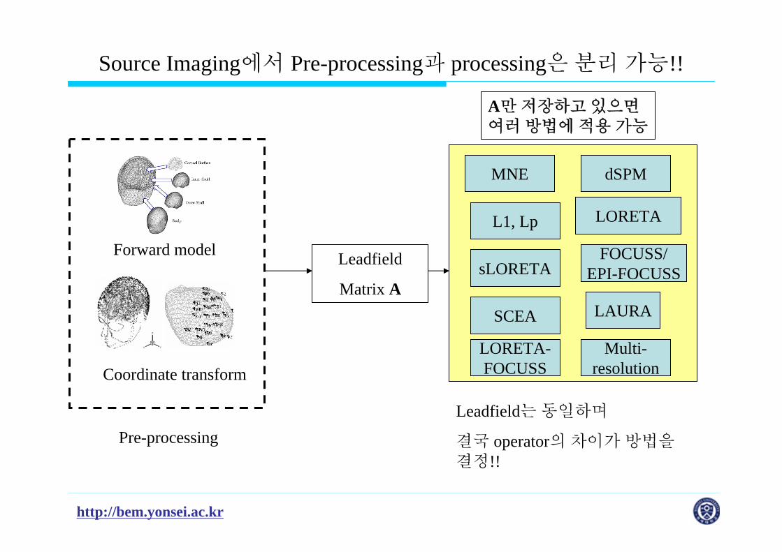
Source Imaging에서 Pre-processing과 processing은분리가능!!
Forward model
Coordinate transform
Pre-processing
Leadfield
Matrix A
A만저장하고있으면여러방법에적용가능
MNE
L1, Lp
sLORETA
SCEA
LORETA
FOCUSS/EPI-FOCUSS
dSPM
LORETA-FOCUSS
Multi-resolution
LAURA
Leadfield는동일하며
결국 operator의 차이가방법을결정!!
http://bem.yonsei.ac.kr
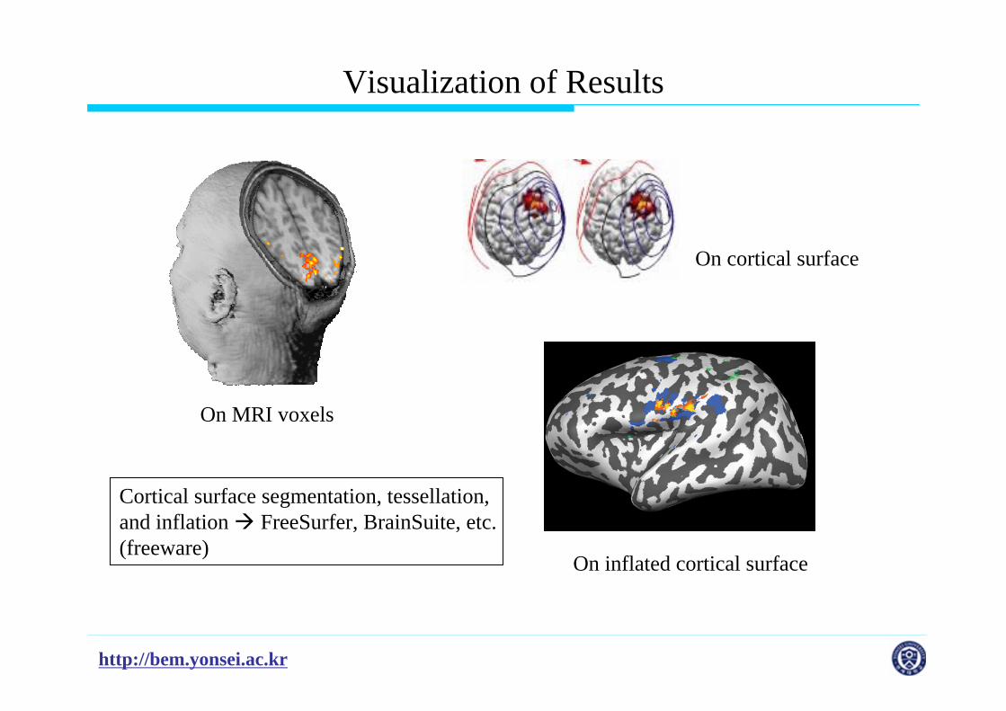
Visualization of Results
On MRI voxels
On cortical surface
On inflated cortical surface
Cortical surface segmentation, tessellation, and inflation FreeSurfer, BrainSuite, etc. (freeware)

http://bem.yonsei.ac.kr
Use of fMRI prior Information
1
0.1 • Liu et al. [1998] revealed that the distortion by the fMRI invisible sources could be reduced considerably by just giving a constant weighting factor to the diagonal terms of source covariance matrix in linear Wiener estimate operator.
Liu AK, Belliveau JW, Dale AM (1998): Spatiotemporal imaging of human brain activity using functional MRI constrained magnetoencephalography data: Monte Carlo simulations. Proc NatlAcad Sci 95:8945-8950.
W = RAt(ARAt + C)-1
The first paper that addressed the possibility of fMRI or PET prior constraint
Dale AM, Sereno M (1993): Improved localization of cortical activity by combining EEG and MEG with MRI surface reconstruction: a linear approach. J Cognit Neurosci 5:162-176.
http://bem.yonsei.ac.kr
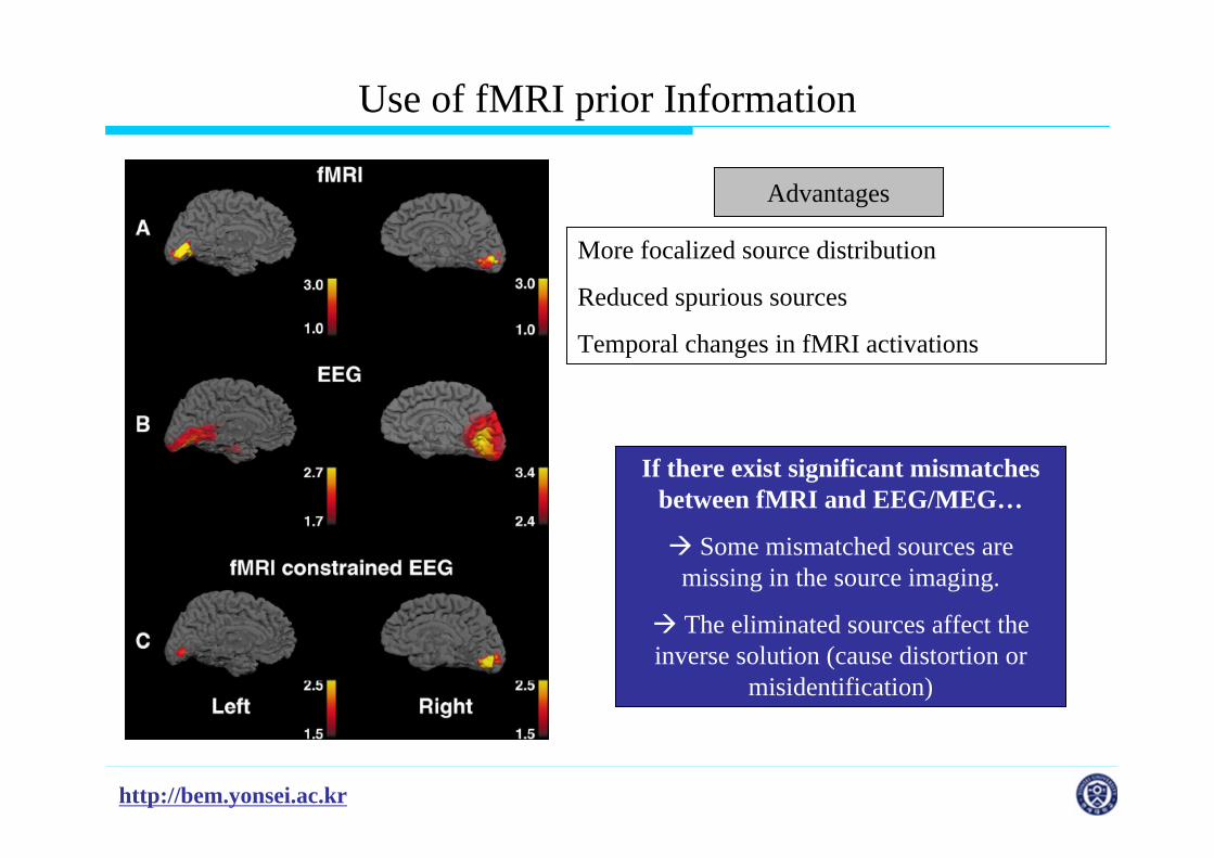
Use of fMRI prior Information
More focalized source distribution
Reduced spurious sources
Temporal changes in fMRI activations
Advantages
If there exist significant mismatches between fMRI and EEG/MEG…
Some mismatched sources are missing in the source imaging.
The eliminated sources affect the inverse solution (cause distortion or
misidentification)
http://bem.yonsei.ac.kr
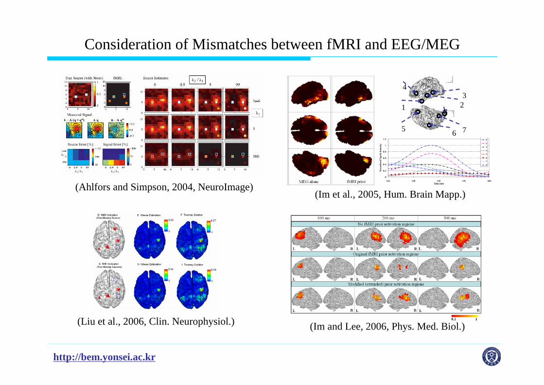
Consideration of Mismatches between fMRI and EEG/MEG
(Ahlfors and Simpson, 2004, NeuroImage)
75
2
4
13
8
6
(Im et al., 2005, Hum. Brain Mapp.)
(Liu et al., 2006, Clin. Neurophysiol.) (Im and Lee, 2006, Phys. Med. Biol.)
http://bem.yonsei.ac.kr 6464/15/15
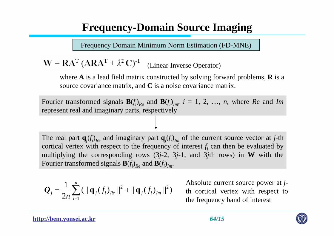
Frequency-Domain Source Imaging
where A is a lead field matrix constructed by solving forward problems, R is a source covariance matrix, and C is a noise covariance matrix.
Fourier transformed signals B(fi)Re and B(fi)Im, i = 1, 2, …, n, where Re and Imrepresent real and imaginary parts, respectively
The real part qj(fi)Re and imaginary part qj(fi)Im of the current source vector at j-thcortical vertex with respect to the frequency of interest fi can then be evaluated by multiplying the corresponding rows (3j-2, 3j-1, and 3jth rows) in W with the Fourier transformed signals B(fi)Re and B(fi)Im.
2 2
1
1 ( || ( ) || || ( ) || )2
n
j j i Re j i Imi
f fn =
= +∑Q q qAbsolute current source power at j-th cortical vertex with respect to the frequency band of interest
(Linear Inverse Operator)
Frequency Domain Minimum Norm Estimation (FD-MNE)

http://bem.yonsei.ac.kr Bioelectromagnetics and Neuroimaging Lab.Bioelectromagnetics and Neuroimaging Lab. Yonsei BME
Real-time Cortical Rhythmic Activity Monitoring System
(Im et al., 2007, Physiol. Meas.)

http://bem.yonsei.ac.kr Bioelectromagnetics and Neuroimaging Lab.Bioelectromagnetics and Neuroimaging Lab. Yonsei BME
Experimental Study (Example 1)
Real-time cortical alpha (8-13 Hz) activity imaging
Subject: YJ (26 years old)
4 frames per second, 16 channels
http://bem.yonsei.ac.kr Bioelectromagnetics and Neuroimaging Lab.Bioelectromagnetics and Neuroimaging Lab. Yonsei BME
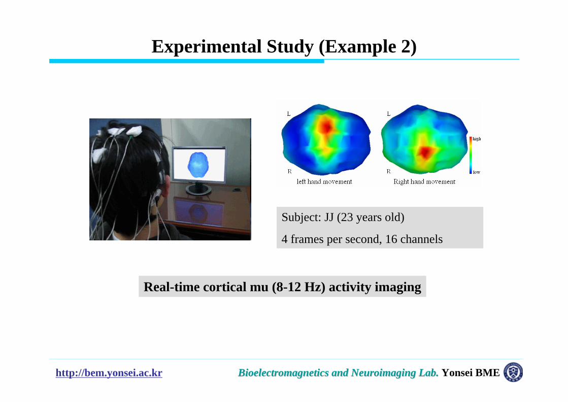
Subject: JJ (23 years old)
4 frames per second, 16 channels
Real-time cortical mu (8-12 Hz) activity imaging
Experimental Study (Example 2)
http://bem.yonsei.ac.kr
Contents
1. Signal Processing
2. Pre-processing
3. Equivalent Current Dipole (ECD) Localization
4. EEG/MEG Source Imaging
5. Commercial/Open Software for EEG/MEG Source Imaging
http://bem.yonsei.ac.kr
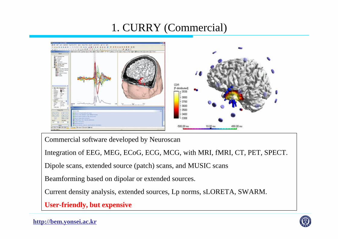
1. CURRY (Commercial)
Commercial software developed by Neuroscan
Integration of EEG, MEG, ECoG, ECG, MCG, with MRI, fMRI, CT, PET, SPECT.
Dipole scans, extended source (patch) scans, and MUSIC scans
Beamforming based on dipolar or extended sources.
Current density analysis, extended sources, Lp norms, sLORETA, SWARM.
User-friendly, but expensive
http://bem.yonsei.ac.kr
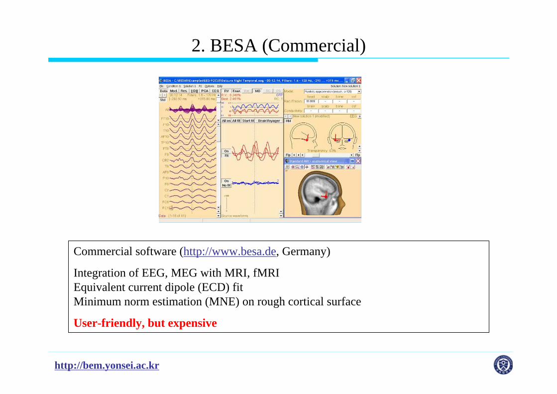
2. BESA (Commercial)
Commercial software (http://www.besa.de, Germany)
Integration of EEG, MEG with MRI, fMRIEquivalent current dipole (ECD) fitMinimum norm estimation (MNE) on rough cortical surface
User-friendly, but expensive
http://bem.yonsei.ac.kr
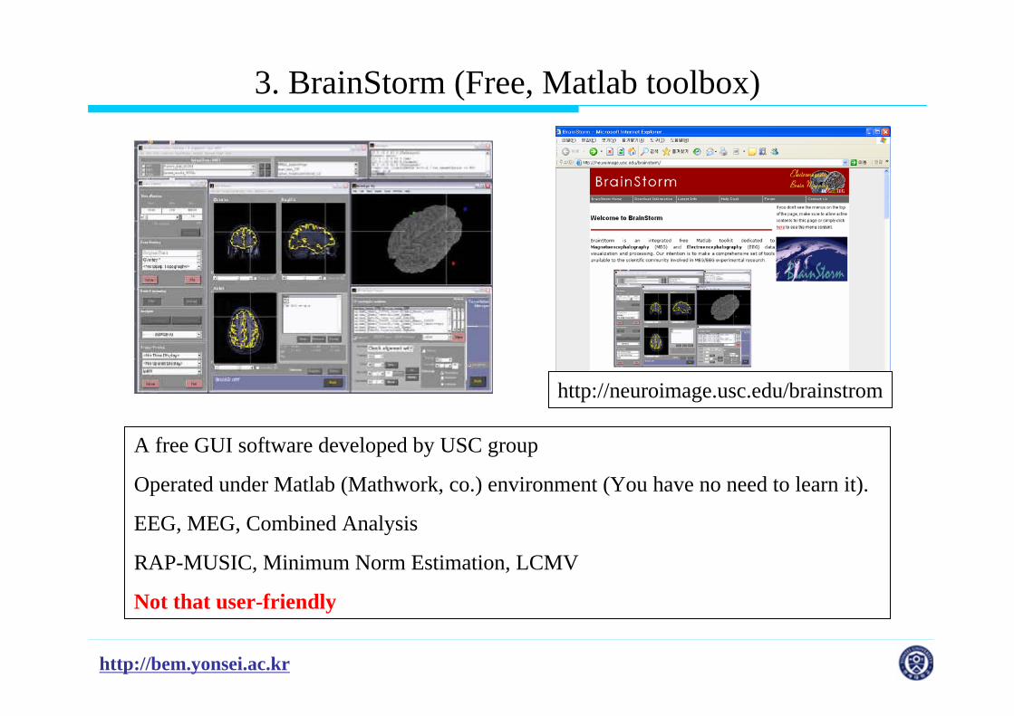
3. BrainStorm (Free, Matlab toolbox)
A free GUI software developed by USC group
Operated under Matlab (Mathwork, co.) environment (You have no need to learn it).
EEG, MEG, Combined Analysis
RAP-MUSIC, Minimum Norm Estimation, LCMV
Not that user-friendly
http://neuroimage.usc.edu/brainstrom
http://bem.yonsei.ac.kr
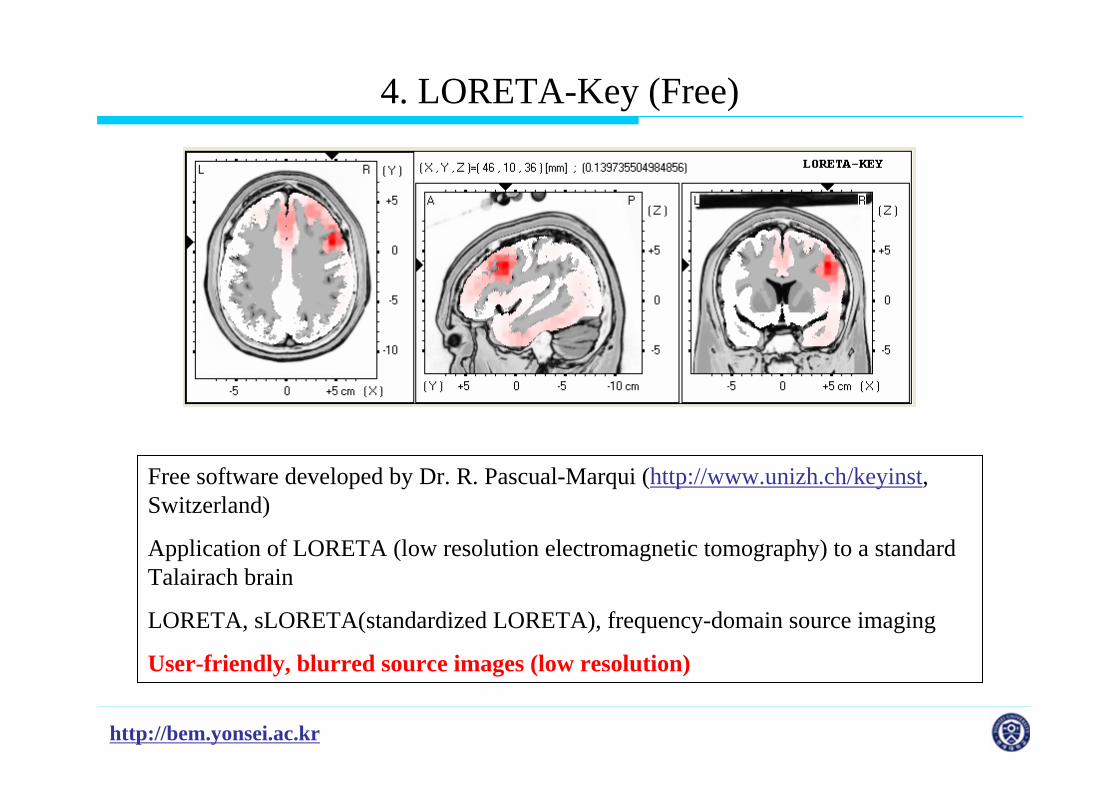
4. LORETA-Key (Free)
Free software developed by Dr. R. Pascual-Marqui (http://www.unizh.ch/keyinst, Switzerland)
Application of LORETA (low resolution electromagnetic tomography) to a standard Talairach brain
LORETA, sLORETA(standardized LORETA), frequency-domain source imaging
User-friendly, blurred source images (low resolution)
http://bem.yonsei.ac.kr Bioelectromagnetics and Neuroimaging Lab.Bioelectromagnetics and Neuroimaging Lab. Yonsei BME
For More Information
Visit our web-page at
http://bem.yonsei.ac.kr
Thank you!
![130125 ich printver.ppt [호환 모드] - Hanyangcone.hanyang.ac.kr/BioEST/Kor/pds/130125_ich_printver.pdf · 2008-02-04 · a periodic brain response elicited by the continuous presentation](https://img.pdfslide.us/doc/110x75/5ee297a1ad6a402d666cf70a/130125-ich-eeoe-hanyangconehanyangackrbioestkorpds130125ichprintverpdf.jpg)