Embed Size (px)
Citation preview
Effects of Multipath Interference
on Radio Positioning Systems
Ramsey Michael Faragher
Department of Physics
Churchill College, University of Cambridge
A thesis submitted for the degree of
Doctor of Philosophy
September 2007

ii

Declaration
This dissertation is the result of work carried out in the Astrophysics Group
of the Cavendish Laboratory, Cambridge, between October 2004 and June 2007.
The work contained in the thesis is my own except where stated otherwise. No
part of this dissertation has been submitted for a degree, diploma or other quali-
fication at this or any other university. The total length of this dissertation does
not exceed sixty thousand words.
Ramsey Faragher
September 2007
iii

This thesis is dedicated to my parents, Pauline and Brian, and to
my brother Paul.
iv

Acknowledgements
I would like to thank my supervisor, Dr. Peter Duffett-Smith, for his friendly
and expert guidance during the last three years, and for giving me the oppor-
tunity to work on such an interesting project. Cambridge Positioning Systems
sponsored this research and I am grateful for their support. I would like to
acknowledge James Brice for his invaluable help in understanding Viterbi decod-
ing and the GSM signal structure. I also want to thank my close friends for
keeping me sane(ish) - Stanislav Shabala, George Vardulakis, Michael Bridges,
Anna Scaife, Emily Curtis, Tom Auld, Jonathan Zwart, Huw Jones, Matt Raskie,
Max Holzner, Paul Rhatigan, David Singerman, Marisa Grillo, Iga Wegorzewska,
Kerry McCann, Vicky Lister, Priya Shah, Friederike Mansfeld, Kirstin Woody,
Avaleigh Milne, Liz Azzato, Alex Gillies and the rest of my basketball team. I
would especially like to thank my girlfriend Ally for her love, patience, and sup-
port during the writing of this thesis. Finally, and most importantly, I want to
thank my parents for their unconditional support, and for putting so much of
their time and money into my education. I could not have reached this point in
my academic career without them.
v

I do not think that the wireless waves I have discovered will have any
practical application.
Heinrich Rudolf Hertz
vi
Abstract
The effects of multipath interference on GSM signal timing stabilities and on ra-
dio positioning systems using the GSM network are examined. Two experimental
methods for accurately measuring signal arrival times are described - the inter-
ferometric technique and the network-synchronised technique. An experimental
apparatus capable of performing measurements on the GSM network to a reso-
lution of 24.5 nanoseconds or 7.35 metres is described. The results of a set of
experiments measuring the timing stability of the received signals from two net-
works suggest that Fine Time Aiding can be provided on one network over time
periods of 3 days or more and on the other over time periods of up to 5 hours.
A set of experiments measuring the positioning error associated with moving an
antenna slowly over sub-wavelength distances indoors is described. Examples of
errors in the region of hundreds of metres are noted for an antenna moving a few
millimetres. The errors are shown to be caused by corruption of the Extended
Training Sequence timing marker in the received signal. The raised-cosine model
is proposed and demonstrates the ability to accurately reproduce experimental
behaviour and determine probable propagation paths. Alternative methods of
determining signal arrival times using the ETS timing marker are proposed and
their accuracies are compared to the usual ‘peak-max’ technique. Finally, the
timing error distributions for rural, suburban, light-urban and mid-urban envi-
ronments are measured. A probability density function model derived from the
raised-cosine model is shown to reproduce the experimental results.
vii
Glossary of Abbreviations
3G. Third Generation.
AOA. Angle Of Arrival.
BCCH. Broadcast Control Channel.
BSIC. Base Station Identity Code.
BTS. Base Transceiver Station.
C/A code. Coarse Acquisition code.
CCH. Control Channel.
CDMA. Code Division Multiple Access.
DCM. Database Correlation Method.
ETS. Extended Training Sequence.
FCB. Frequency Control Burst.
FDMA. Frequency Division Multiple Access.
FH. Frequency Hopping.
FTA. Fine Time Aiding.
FRK-H. The model of Rubidium Oscillator used in this project.
GLONASS. GLObal NAvigation Satellite System.
GNSS. Global Navigation Satellite System.
GPIB. General Purpose Interface Bus.
GPS. Global Positioning System.
GSM. Group Speciale Mobile
ILS. Instrument Landing System.
LORAN. LOng RAnge Navigation.
LOS. Line Of Sight.
MCXO. Microprocessor Controlled Crystal Oscillator.
viii
NAVSTAR. NAVigation Satellite Timing And Ranging.
OCXO. Oven Controlled Crystal Oscillator.
P code. Precise code.
PN code. Pseudorandom Number code.
RbO. Rubidium Oscillator.
RDF. Radio Direction Finder.
RFS. Rubidium Frequency Standard.
SA. Selective Availability.
SCB. SynChronisation Burst.
SCH. SynChronisation Channel.
SNR. Signal to Noise Ratio.
TCXO. Temperature Controlled Crystal Oscillator.
TDOA. Time Difference Of Arrival.
TDMA. Time Division Multiple Access.
TOA. Time Of Arrival.
TOF. Time Of Flight.
TTFF. Time To First Fix.
UMTS. Universal Mobile Telecommunications System.
UPS. Uninterruptible Power Supply.
VHF. Very High Frequency.
VLF. Very Low Frequency.
VOR. Very High Frequency Omni-directional Radio Ranging.
XO. Crystal Oscillator.
ix

x
Contents
1 Introduction to radio positioning 1
1.1 Local radio positioning . . . . . . . . . . . . . . . . . . . . . . . . 3
1.2 Cell-phone positioning . . . . . . . . . . . . . . . . . . . . . . . . 9
1.2.1 Cell-ID . . . . . . . . . . . . . . . . . . . . . . . . . . . . . 11
1.2.2 Database Correlation . . . . . . . . . . . . . . . . . . . . . 12
1.2.3 Enhanced Observed Time Difference . . . . . . . . . . . . 13
1.2.4 Matrix . . . . . . . . . . . . . . . . . . . . . . . . . . . . . 13
1.2.5 Enhanced GPS . . . . . . . . . . . . . . . . . . . . . . . . 14
1.2.5.1 Autonomous start . . . . . . . . . . . . . . . . . 17
1.2.5.2 Cold start . . . . . . . . . . . . . . . . . . . . . . 18
1.2.5.3 Warm and hot starts . . . . . . . . . . . . . . . . 18
1.2.5.4 Fine Time Aiding . . . . . . . . . . . . . . . . . . 18
1.3 Multipath interference . . . . . . . . . . . . . . . . . . . . . . . . 19
1.4 Contributions to this field of research . . . . . . . . . . . . . . . . 20
1.5 Thesis outline . . . . . . . . . . . . . . . . . . . . . . . . . . . . . 21
2 Timing stability 23
2.1 Allan Variance . . . . . . . . . . . . . . . . . . . . . . . . . . . . 24
2.2 Oscillators . . . . . . . . . . . . . . . . . . . . . . . . . . . . . . . 32
2.2.1 Crystal oscillators . . . . . . . . . . . . . . . . . . . . . . . 34
2.2.2 Temperature-compensated crystal oscillators . . . . . . . . 37
2.2.3 Oven-controlled crystal oscillators . . . . . . . . . . . . . . 37
xi
CONTENTS
2.2.4 Microcomputer-controlled crystal oscillators . . . . . . . . 38
2.3 Atomic oscillators . . . . . . . . . . . . . . . . . . . . . . . . . . . 39
2.3.1 Rubidium oscillators . . . . . . . . . . . . . . . . . . . . . 40
2.3.2 Caesium beam oscillators . . . . . . . . . . . . . . . . . . . 44
2.3.3 Hydrogen masers . . . . . . . . . . . . . . . . . . . . . . . 45
2.3.4 Caesium fountains . . . . . . . . . . . . . . . . . . . . . . 47
2.3.5 Optical atomic clocks . . . . . . . . . . . . . . . . . . . . . 48
2.4 Measurements with two Rb frequency standards . . . . . . . . . . 48
2.5 Measurements of the stabilities of FRK-H Rb oscillators . . . . . 49
2.6 Conclusions . . . . . . . . . . . . . . . . . . . . . . . . . . . . . . 51
3 Time of flight measurements on cellular networks 55
3.1 Methods . . . . . . . . . . . . . . . . . . . . . . . . . . . . . . . . 55
3.1.1 Interferometric method . . . . . . . . . . . . . . . . . . . . 55
3.1.2 Network-synchronised method . . . . . . . . . . . . . . . . 56
3.2 The Apparatus . . . . . . . . . . . . . . . . . . . . . . . . . . . . 58
3.2.1 Radio frequency digitiser . . . . . . . . . . . . . . . . . . . 59
3.2.2 Triggering and synchronisation . . . . . . . . . . . . . . . 59
3.2.3 Uninterruptible power supplies . . . . . . . . . . . . . . . . 60
3.3 Data storage and analysis . . . . . . . . . . . . . . . . . . . . . . 60
3.3.1 Sampling theory . . . . . . . . . . . . . . . . . . . . . . . 61
3.3.2 MATLAB driven data capture . . . . . . . . . . . . . . . . 63
3.3.3 Cross correlation . . . . . . . . . . . . . . . . . . . . . . . 66
3.3.3.1 The ambiguity function . . . . . . . . . . . . . . 66
3.4 Anatomy of a GSM signal . . . . . . . . . . . . . . . . . . . . . . 68
3.4.1 GSM digital encoding . . . . . . . . . . . . . . . . . . . . 71
3.5 Anatomy of a CDMA signal . . . . . . . . . . . . . . . . . . . . . 72
3.6 The Experiments . . . . . . . . . . . . . . . . . . . . . . . . . . . 73
3.6.1 Preparation . . . . . . . . . . . . . . . . . . . . . . . . . . 73
3.6.2 Surveying . . . . . . . . . . . . . . . . . . . . . . . . . . . 74
xii
CONTENTS
3.6.3 Post-processing . . . . . . . . . . . . . . . . . . . . . . . . 74
4 GSM Network Stability 85
4.1 Method and apparatus . . . . . . . . . . . . . . . . . . . . . . . . 85
4.1.1 Calibration . . . . . . . . . . . . . . . . . . . . . . . . . . 87
4.2 Results and discussion . . . . . . . . . . . . . . . . . . . . . . . . 88
4.2.1 900 MHz Network . . . . . . . . . . . . . . . . . . . . . . . 93
4.2.2 1800 MHz Network . . . . . . . . . . . . . . . . . . . . . . 98
4.3 Conclusions . . . . . . . . . . . . . . . . . . . . . . . . . . . . . . 101
5 The effects of indoor multipath environments on timing stability103
5.1 Method and apparatus . . . . . . . . . . . . . . . . . . . . . . . . 103
5.2 Results and discussions . . . . . . . . . . . . . . . . . . . . . . . . 104
5.2.1 Roof experiment . . . . . . . . . . . . . . . . . . . . . . . 105
5.2.2 Roof Laboratory Tests . . . . . . . . . . . . . . . . . . . . 110
5.2.3 Electronics Laboratory tests . . . . . . . . . . . . . . . . . 117
5.2.3.1 Spatial and temporal variations . . . . . . . . . . 120
5.3 Conclusions . . . . . . . . . . . . . . . . . . . . . . . . . . . . . . 126
6 Modelling the effects of indoor multipath environments on tim-
ing stability 127
6.1 Modelling cross-correlation peak distortions . . . . . . . . . . . . 127
6.1.1 Received Signal Interference model . . . . . . . . . . . . . 128
6.1.2 Cross-Correlation Peak Interference model . . . . . . . . . 128
6.1.3 Results of simulations . . . . . . . . . . . . . . . . . . . . 129
6.2 Determining signal arrival times . . . . . . . . . . . . . . . . . . . 138
6.3 Conclusions . . . . . . . . . . . . . . . . . . . . . . . . . . . . . . 144
7 A study of the timing errors encountered when performing radio-
location using the GSM network 147
7.1 Definitions of environment . . . . . . . . . . . . . . . . . . . . . . 148
7.2 Apparatus . . . . . . . . . . . . . . . . . . . . . . . . . . . . . . . 149
xiii
CONTENTS
7.2.1 GPS . . . . . . . . . . . . . . . . . . . . . . . . . . . . . . 149
7.2.2 GPS accuracy and errors . . . . . . . . . . . . . . . . . . . 150
7.3 Method . . . . . . . . . . . . . . . . . . . . . . . . . . . . . . . . 152
7.3.1 Indoor mapping accuracy . . . . . . . . . . . . . . . . . . 155
7.4 Results . . . . . . . . . . . . . . . . . . . . . . . . . . . . . . . . . 155
7.4.1 Error analysis . . . . . . . . . . . . . . . . . . . . . . . . . 159
7.5 Modelling the timing error distributions . . . . . . . . . . . . . . 161
7.5.1 Fitting the free parameters . . . . . . . . . . . . . . . . . . 166
7.6 Conclusions . . . . . . . . . . . . . . . . . . . . . . . . . . . . . . 172
8 Summary and further work 175
8.1 The experimental apparatus . . . . . . . . . . . . . . . . . . . . . 175
8.2 The experimental methods . . . . . . . . . . . . . . . . . . . . . . 175
8.3 GSM network timing stabilities . . . . . . . . . . . . . . . . . . . 176
8.4 GSM network timing stabilities in indoor multipath environments 176
8.5 GSM radio location timing error distributions in various environ-
ments . . . . . . . . . . . . . . . . . . . . . . . . . . . . . . . . . 177
8.6 Further work . . . . . . . . . . . . . . . . . . . . . . . . . . . . . 178
A Distributions of A, φ and α 181
A.1 Distribution of φ . . . . . . . . . . . . . . . . . . . . . . . . . . . 182
A.2 Distribution of α . . . . . . . . . . . . . . . . . . . . . . . . . . . 183
A.3 Distribution of A . . . . . . . . . . . . . . . . . . . . . . . . . . . 183
References 199
xiv

List of Figures
1.1 Sketch showing the geometries involved with the Angle Of Arrival,
Time Of Arrival and signal strength positioning methods. . . . . . 2
1.2 Sketch showing the hyperbolic geometry involved with the TDOA
positioning method. . . . . . . . . . . . . . . . . . . . . . . . . . . 5
1.3 Plot showing the variation in candidate locations for a GPS re-
ceiver position using the weak-signal method as the satellites move
through their orbits. . . . . . . . . . . . . . . . . . . . . . . . . . 10
1.4 Plot showing the cross-correlation function resulting from search-
ing a frequency range for a given PN code . . . . . . . . . . . . . 15
1.5 Sketch demonstrating the benefit of having accurate estimates of
the positions of the PN codes in the received satellite broadcasts . 17
2.1 Sketch showing the types of error affecting an oscillator’s frequency 25
2.2 Plot of a series of phase samples versus time. . . . . . . . . . . . . 27
2.3 Idealised Allan deviation Plot . . . . . . . . . . . . . . . . . . . . 30
2.4 Allan deviation plot for various oscillators. . . . . . . . . . . . . . 31
2.5 Plot showing a simple electrical circuit which displays oscillatory
behaviour. . . . . . . . . . . . . . . . . . . . . . . . . . . . . . . . 33
2.6 Plot showing the transfer of energy in a tank circuit during its
oscillatory cycles. . . . . . . . . . . . . . . . . . . . . . . . . . . . 33
2.7 Plot showing nomalised resonance curves for oscillators with dif-
ferent Q values. . . . . . . . . . . . . . . . . . . . . . . . . . . . . 35
xv
LIST OF FIGURES
2.8 The equivalent electrical circuit for a crystal resonator . . . . . . 35
2.9 A circuit diagram for a crystal oscillator . . . . . . . . . . . . . . 36
2.10 Plot showing the frequency variations with temperature for three
crystal oscillator systems. . . . . . . . . . . . . . . . . . . . . . . 38
2.11 Schematic diagram of a Rubidium frequency standard. . . . . . . 42
2.12 Schematic diagram of a Caesium beam frequency standard. . . . . 45
2.13 Schematic diagram of a Hydrogen maser frequency standard. . . . 47
2.14 Schematic diagram of the apparatus used to measure the stability
of an FRK-H Rb oscillator. . . . . . . . . . . . . . . . . . . . . . . 50
2.15 Allan deviation plots for an Efratom FRK-H Rb oscillator and for
an OCXO. . . . . . . . . . . . . . . . . . . . . . . . . . . . . . . . 52
2.16 The phase differences between the 10MHz outputs of two Rubid-
ium oscillators in four experiments. . . . . . . . . . . . . . . . . . 53
3.1 The experimental apparatus . . . . . . . . . . . . . . . . . . . . . 58
3.2 A sample of data showing the signal-to-noise ratio . . . . . . . . . 63
3.3 Sampling theory . . . . . . . . . . . . . . . . . . . . . . . . . . . . 64
3.4 The ETS ambiguity function . . . . . . . . . . . . . . . . . . . . . 67
3.5 GSM Framing . . . . . . . . . . . . . . . . . . . . . . . . . . . . . 69
3.6 GSM Bursts . . . . . . . . . . . . . . . . . . . . . . . . . . . . . . 70
3.7 Post-processing flowchart . . . . . . . . . . . . . . . . . . . . . . . 75
3.8 A description of the GSM modulation and encoding techniques,
and the BSIC and frame number decoding process . . . . . . . . . 77
3.9 A description of the GSM modulation and encoding techniques,
and the BSIC and frame number decoding process (continued) . . 78
3.10 A description of the GSM modulation and encoding techniques,
and the BSIC and frame number decoding process (continued) . . 79
3.11 A description of the GSM modulation and encoding techniques,
and the BSIC and frame number decoding process (continued) . . 80
3.12 A cross-correlation profile generated using the interferometric method 82
xvi
LIST OF FIGURES
3.13 A cross-correlation profile generated using the network-synchronised
method . . . . . . . . . . . . . . . . . . . . . . . . . . . . . . . . 83
4.1 A picture showing the antenna above the roof of the Cavendish
Laboratory . . . . . . . . . . . . . . . . . . . . . . . . . . . . . . 86
4.2 Sketch showing the experimental setup used to produce the cali-
bration Allan Deviation curves . . . . . . . . . . . . . . . . . . . . 88
4.3 Plot showing the Allan deviation curves produced by an internally-
and externally-locked Racal GSM signal generator. . . . . . . . . 89
4.4 Plots showing the variation in relative signal arrival times from a
GSM base station broadcasting in the 900 MHz waveband. . . . . 90
4.5 Plot showing the variation in signal arrival times from a GSM base
station broadcasting in the 1800 MHz waveband. . . . . . . . . . 91
4.6 The Fourier transform of the data given in Figure 4.4. . . . . . . . 92
4.7 The Fourier transform of the data given in Figure 4.5. . . . . . . . 92
4.8 The Allan deviation plots for the base stations on the 900MHz
network . . . . . . . . . . . . . . . . . . . . . . . . . . . . . . . . 94
4.9 Map of Cambridgeshire showing the positions of the base stations
studied and the Cavendish Laboratory . . . . . . . . . . . . . . . 95
4.10 The timing data and Allan deviation curves from the 900 MHz
GSM base station represented by Curve ‘C’ in Figure 4.8 . . . . . 97
4.11 The Allan deviation plots for the base stations on the 1800MHz
network . . . . . . . . . . . . . . . . . . . . . . . . . . . . . . . . 99
4.12 Plot comparing the timing errors for three base stations. . . . . . 100
5.1 A view of the BTS from the roof of the Rutherford building . . . 106
5.2 A view of the BTS from the first position of the antenna during
the initial experiment on the roof of the Rutherford building . . . 107
5.3 Diagram illustrating the first Fresnel zone for a transmitter-receiver
separation of 1,200 metres and operating with a wavelength of 30
centimetres . . . . . . . . . . . . . . . . . . . . . . . . . . . . . . 108
xvii
LIST OF FIGURES
5.4 Plot showing the data from the roof experiment. . . . . . . . . . . 109
5.5 Plot showing sample SCB peaks from the roof experiment . . . . 110
5.6 Plot showing multipath behaviour recorded inside the Roof Labo-
ratory . . . . . . . . . . . . . . . . . . . . . . . . . . . . . . . . . 112
5.7 Plot showing multipath behaviour recorded inside the Roof Labo-
ratory . . . . . . . . . . . . . . . . . . . . . . . . . . . . . . . . . 114
5.8 Plot showing multipath behaviour recorded inside the Roof Labo-
ratory . . . . . . . . . . . . . . . . . . . . . . . . . . . . . . . . . 115
5.9 Sketch demonstrating how sharp spikes in timing error can be pro-
duced by SCB peaks deformed by multipath interference . . . . . 116
5.10 Plot showing the signal stability recorded inside the Rutherford
Building during the night . . . . . . . . . . . . . . . . . . . . . . 117
5.11 Plot showing the consistency of the multipath behaviour recorded
inside a room in the Rutherford building. . . . . . . . . . . . . . . 119
5.12 Plot showing the multipath behaviour recorded inside the Ruther-
ford building over a small area. . . . . . . . . . . . . . . . . . . . 120
5.13 Plot showing the moduli of ten consecutive SCB peaks recorded
during an indoor survey . . . . . . . . . . . . . . . . . . . . . . . 121
5.14 Scatter plots showing the correlation between temporal and the
apparent spatial multipath variation. . . . . . . . . . . . . . . . . 123
5.15 Plot showing multipath behaviour recorded inside the Rutherford
building by a slow moving antenna. . . . . . . . . . . . . . . . . . 124
5.16 Plot showing the timing variations recorded in the main corridor
of the Rutherford building for a slow moving antenna. . . . . . . . 125
6.1 Plot showing a simulation of the Roof Laboratory experiment . . 130
6.2 Plot showing a simulation of the Roof Laboratory experiment . . 131
6.3 Picture showing the view from the Roof Laboratory window . . . 132
6.4 Plot showing a simulation of the Roof Laboratory experiment. . . 133
6.5 Plot showing a simulation of the Electronics Laboratory experiment.134
xviii
LIST OF FIGURES
6.6 Plot showing a simulation of the Electronics Laboratory experi-
ment with random phases on reception. . . . . . . . . . . . . . . . 136
6.7 Plot showing a simulation of the Electronics Laboratory experi-
ment with random amplitudes on reception. . . . . . . . . . . . . 137
6.8 Plot showing a simulation of the Electronics Laboratory experi-
ment with random amplitudes and measurement noise on reception.138
6.9 Plot showing methods of determining a signal arrival time using
the SCB peak. . . . . . . . . . . . . . . . . . . . . . . . . . . . . . 139
6.10 Plots showing tests of the three signal-arrival techniques using sim-
ulated data. . . . . . . . . . . . . . . . . . . . . . . . . . . . . . . 141
6.11 Plots showing tests of the three signal-arrival techniques using two
sets of data gathered using an indoor receiver. . . . . . . . . . . . 142
6.12 Plot showing tests of the three signal-arrival techniques using the
data from the initial roof experiment. . . . . . . . . . . . . . . . . 143
7.1 Plot showing the effects of good and bad satellite geometry on the
accuracy of a GPS position . . . . . . . . . . . . . . . . . . . . . . 151
7.2 Plot showing the distribution of GPS positions recorded in a fixed
position on the Cavendish Laboratory roof at 2 pm and 5 pm over
many days and weather conditions. . . . . . . . . . . . . . . . . . 153
7.3 Plot showing the use of Pythagoras’ theorem in calculating the
distance from a base station using the signal flight time. . . . . . 154
7.4 Plots of the normalised histograms of the timing error for each
environment . . . . . . . . . . . . . . . . . . . . . . . . . . . . . . 156
7.5 Diagram showing the floor plan of the indoor environment used in
the survey. . . . . . . . . . . . . . . . . . . . . . . . . . . . . . . . 158
7.6 Comparison of the modulus of the GSM ETS auto-correlation peak
and a truncated raised-cosine function . . . . . . . . . . . . . . . 162
7.7 Plot showing how the superposition of two displaced and out-of-
phase cross-correlation peaks can result in a distorted function. . . 163
xix
LIST OF FIGURES
7.8 Plot showing the effect of varying σy in the model . . . . . . . . . 167
7.9 Plot showing the effect of varying R in the model . . . . . . . . . 167
7.10 Plot showing the effect of varying p in the model . . . . . . . . . . 168
7.11 Plot showing the characteristic delays in the outdoor environments 169
7.12 Plots showing the rural data set with the multipath model overlaid 170
7.13 Plots showing the suburban data set with the multipath model
overlaid . . . . . . . . . . . . . . . . . . . . . . . . . . . . . . . . 170
7.14 Plots showing the light-urban data set with the multipath model
overlaid. . . . . . . . . . . . . . . . . . . . . . . . . . . . . . . . . 171
7.15 Plots showing the mid-urban data set with the multipath model
overlaid. . . . . . . . . . . . . . . . . . . . . . . . . . . . . . . . . 171
7.16 Plots showing the indoor data set with an adjusted multipath
model overlaid . . . . . . . . . . . . . . . . . . . . . . . . . . . . 172
A.1 Diagram showing the parameters for considering Fresnel diffraction
at a knife edge . . . . . . . . . . . . . . . . . . . . . . . . . . . . . 184
A.2 Plots of the signal amplitudes after diffraction down to points of
interest from a single knife edge for various distances from a 15
metre tall BTS . . . . . . . . . . . . . . . . . . . . . . . . . . . . 186
A.3 A plane wave incident onto a plane boundary . . . . . . . . . . . 187
A.4 Plots of the reflection coefficients for vertically polarised 900MHz
GSM signals incident on brick and concrete surfaces . . . . . . . . 188
A.5 Plots showing the received signal amplitude (relative to the unob-
structed signal) for two propagation mechanisms. . . . . . . . . . 190
A.6 Plots showing the correlation between S1 and S2 for the four po-
tential distributions of A and the distributions of α and φ. . . . . 192
xx
Chapter 1
Introduction to radio positioning
This thesis examines the effects of multipath interference on radio positioning
techniques, specifically those that can be employed on the GSM cellular network
using signal arrival time measurements. The ability to locate a person or object
using radio waves holds great appeal for many applications such as safety and
security applications, personal navigation, the provision of location-based services
and the tracking of people or goods. All cellular radio-positioning systems require
a method of determining a user’s position relative to a set of signal sources at
known locations. This position can be determined using one or more of the
following basic methods:
Angle Of Arrival (AOA). The user’s position can be determined by considering
the direction to each source (triangulation).
Time Of Arrival (TOA). The user’s position can be determined by calculating the
distance (or difference in distances) to each source, inferred from measurements
of the signal arrival times (or differences in arrival times). The distance to a
source is directly proportional to the signal flight time for a signal propagating
in a given medium.
Signal strength. Signal strength decreases predictably in free space with distance
from the source. The received signal strengths from a number of sources can be
used to establish estimates of the distances to the sources.
1
1. INTRODUCTION TO RADIO POSITIONING
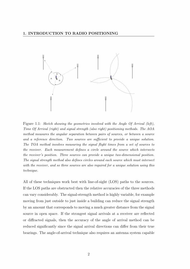
Figure 1.1: Sketch showing the geometries involved with the Angle Of Arrival (left),Time Of Arrival (right) and signal strength (also right) positioning methods. The AOAmethod measures the angular separation between pairs of sources, or between a sourceand a reference direction. Two sources are sufficient to provide a unique solution.The TOA method involves measuring the signal flight times from a set of sources tothe receiver. Each measurement defines a circle around the source which intersectsthe receiver’s position. Three sources can provide a unique two-dimensional position.The signal strength method also defines circles around each source which must intersectwith the receiver, and so three sources are also required for a unique solution using thistechnique.
All of these techniques work best with line-of-sight (LOS) paths to the sources.
If the LOS paths are obstructed then the relative accuracies of the three methods
can vary considerably. The signal-strength method is highly variable, for example
moving from just outside to just inside a building can reduce the signal strength
by an amount that corresponds to moving a much greater distance from the signal
source in open space. If the strongest signal arrivals at a receiver are reflected
or diffracted signals, then the accuracy of the angle of arrival method can be
reduced significantly since the signal arrival directions can differ from their true
bearings. The angle-of-arrival technique also requires an antenna system capable
2
1.1 Local radio positioning
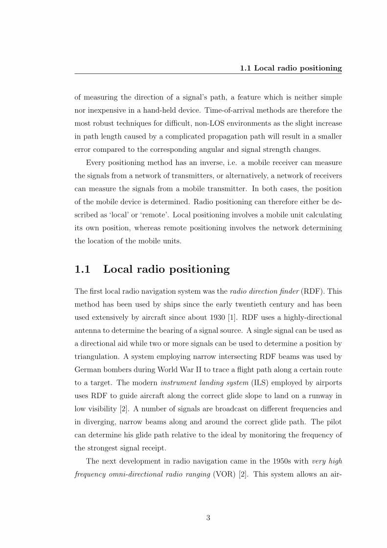
of measuring the direction of a signal’s path, a feature which is neither simple
nor inexpensive in a hand-held device. Time-of-arrival methods are therefore the
most robust techniques for difficult, non-LOS environments as the slight increase
in path length caused by a complicated propagation path will result in a smaller
error compared to the corresponding angular and signal strength changes.
Every positioning method has an inverse, i.e. a mobile receiver can measure
the signals from a network of transmitters, or alternatively, a network of receivers
can measure the signals from a mobile transmitter. In both cases, the position
of the mobile device is determined. Radio positioning can therefore either be de-
scribed as ‘local’ or ‘remote’. Local positioning involves a mobile unit calculating
its own position, whereas remote positioning involves the network determining
the location of the mobile units.
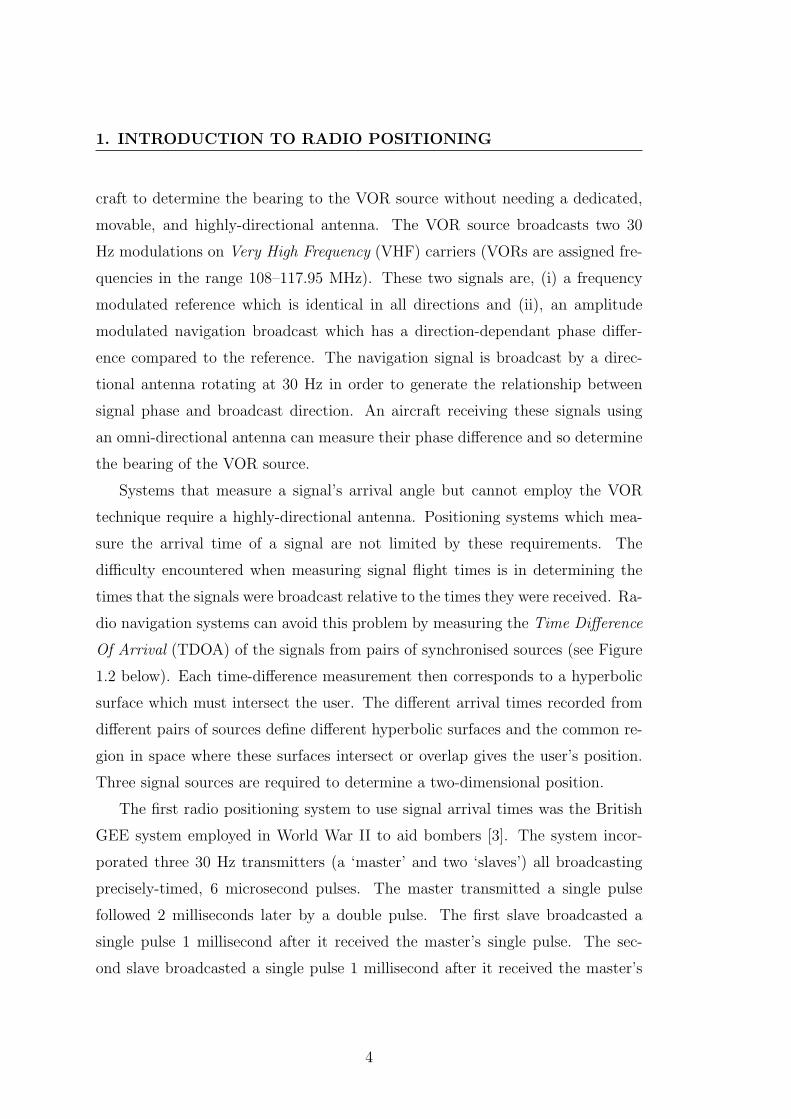
1.1 Local radio positioning
The first local radio navigation system was the radio direction finder (RDF). This
method has been used by ships since the early twentieth century and has been
used extensively by aircraft since about 1930 [1]. RDF uses a highly-directional
antenna to determine the bearing of a signal source. A single signal can be used as
a directional aid while two or more signals can be used to determine a position by
triangulation. A system employing narrow intersecting RDF beams was used by
German bombers during World War II to trace a flight path along a certain route
to a target. The modern instrument landing system (ILS) employed by airports
uses RDF to guide aircraft along the correct glide slope to land on a runway in
low visibility [2]. A number of signals are broadcast on different frequencies and
in diverging, narrow beams along and around the correct glide path. The pilot
can determine his glide path relative to the ideal by monitoring the frequency of
the strongest signal receipt.
The next development in radio navigation came in the 1950s with very high
frequency omni-directional radio ranging (VOR) [2]. This system allows an air-
3
1. INTRODUCTION TO RADIO POSITIONING
craft to determine the bearing to the VOR source without needing a dedicated,
movable, and highly-directional antenna. The VOR source broadcasts two 30
Hz modulations on Very High Frequency (VHF) carriers (VORs are assigned fre-
quencies in the range 108–117.95 MHz). These two signals are, (i) a frequency
modulated reference which is identical in all directions and (ii), an amplitude
modulated navigation broadcast which has a direction-dependant phase differ-
ence compared to the reference. The navigation signal is broadcast by a direc-
tional antenna rotating at 30 Hz in order to generate the relationship between
signal phase and broadcast direction. An aircraft receiving these signals using
an omni-directional antenna can measure their phase difference and so determine
the bearing of the VOR source.
Systems that measure a signal’s arrival angle but cannot employ the VOR
technique require a highly-directional antenna. Positioning systems which mea-
sure the arrival time of a signal are not limited by these requirements. The
difficulty encountered when measuring signal flight times is in determining the
times that the signals were broadcast relative to the times they were received. Ra-
dio navigation systems can avoid this problem by measuring the Time Difference
Of Arrival (TDOA) of the signals from pairs of synchronised sources (see Figure
1.2 below). Each time-difference measurement then corresponds to a hyperbolic
surface which must intersect the user. The different arrival times recorded from
different pairs of sources define different hyperbolic surfaces and the common re-
gion in space where these surfaces intersect or overlap gives the user’s position.
Three signal sources are required to determine a two-dimensional position.
The first radio positioning system to use signal arrival times was the British
GEE system employed in World War II to aid bombers [3]. The system incor-
porated three 30 Hz transmitters (a ‘master’ and two ‘slaves’) all broadcasting
precisely-timed, 6 microsecond pulses. The master transmitted a single pulse
followed 2 milliseconds later by a double pulse. The first slave broadcasted a
single pulse 1 millisecond after it received the master’s single pulse. The sec-
ond slave broadcasted a single pulse 1 millisecond after it received the master’s
4
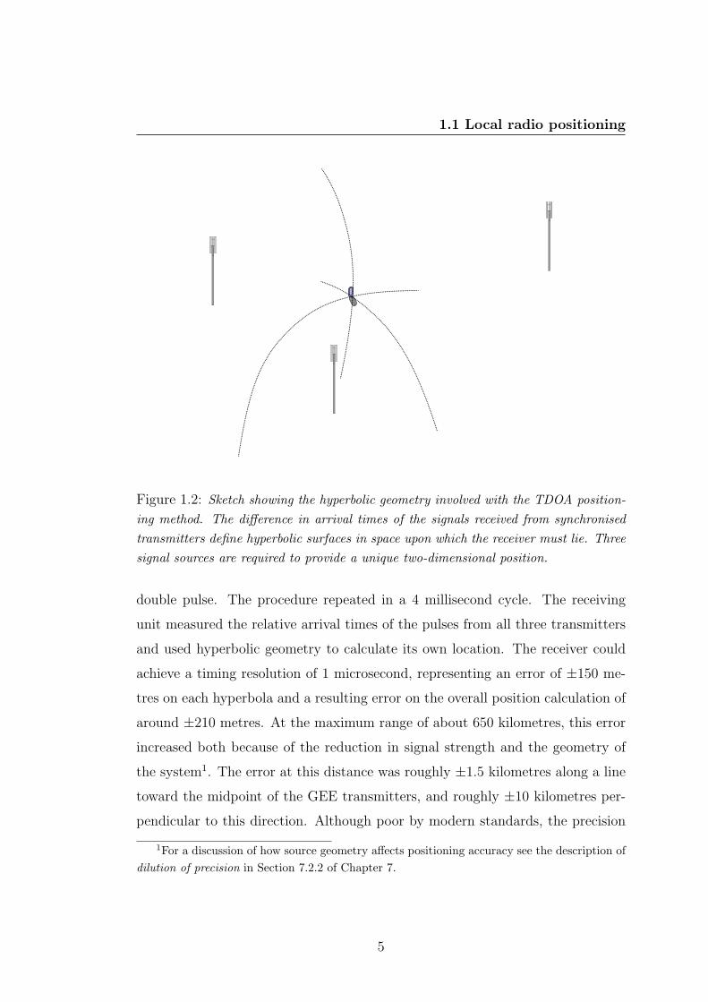
1.1 Local radio positioning
Figure 1.2: Sketch showing the hyperbolic geometry involved with the TDOA position-ing method. The difference in arrival times of the signals received from synchronisedtransmitters define hyperbolic surfaces in space upon which the receiver must lie. Threesignal sources are required to provide a unique two-dimensional position.
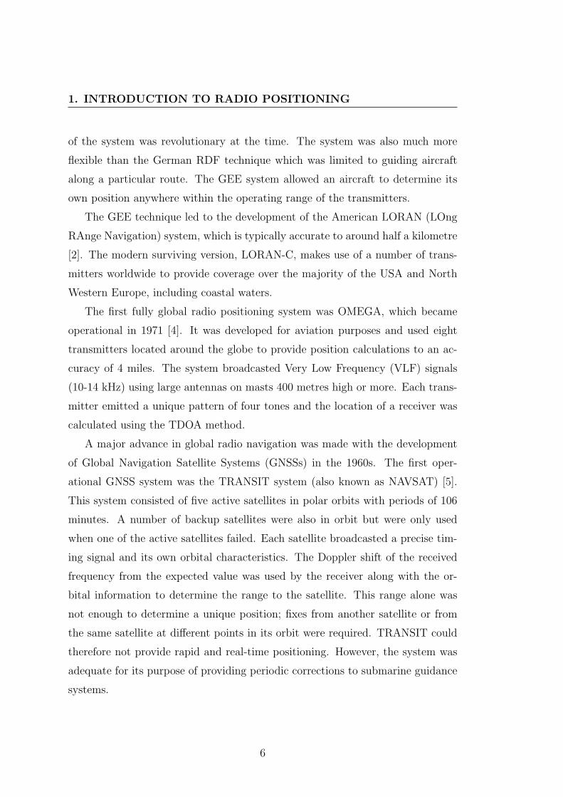
double pulse. The procedure repeated in a 4 millisecond cycle. The receiving
unit measured the relative arrival times of the pulses from all three transmitters
and used hyperbolic geometry to calculate its own location. The receiver could
achieve a timing resolution of 1 microsecond, representing an error of ±150 me-
tres on each hyperbola and a resulting error on the overall position calculation of
around ±210 metres. At the maximum range of about 650 kilometres, this error
increased both because of the reduction in signal strength and the geometry of
the system1. The error at this distance was roughly ±1.5 kilometres along a line
toward the midpoint of the GEE transmitters, and roughly ±10 kilometres per-
pendicular to this direction. Although poor by modern standards, the precision
1For a discussion of how source geometry affects positioning accuracy see the description ofdilution of precision in Section 7.2.2 of Chapter 7.
5
1. INTRODUCTION TO RADIO POSITIONING
of the system was revolutionary at the time. The system was also much more
flexible than the German RDF technique which was limited to guiding aircraft
along a particular route. The GEE system allowed an aircraft to determine its
own position anywhere within the operating range of the transmitters.
The GEE technique led to the development of the American LORAN (LOng
RAnge Navigation) system, which is typically accurate to around half a kilometre
[2]. The modern surviving version, LORAN-C, makes use of a number of trans-
mitters worldwide to provide coverage over the majority of the USA and North
Western Europe, including coastal waters.
The first fully global radio positioning system was OMEGA, which became
operational in 1971 [4]. It was developed for aviation purposes and used eight
transmitters located around the globe to provide position calculations to an ac-
curacy of 4 miles. The system broadcasted Very Low Frequency (VLF) signals
(10-14 kHz) using large antennas on masts 400 metres high or more. Each trans-
mitter emitted a unique pattern of four tones and the location of a receiver was
calculated using the TDOA method.
A major advance in global radio navigation was made with the development
of Global Navigation Satellite Systems (GNSSs) in the 1960s. The first oper-
ational GNSS system was the TRANSIT system (also known as NAVSAT) [5].
This system consisted of five active satellites in polar orbits with periods of 106
minutes. A number of backup satellites were also in orbit but were only used
when one of the active satellites failed. Each satellite broadcasted a precise tim-
ing signal and its own orbital characteristics. The Doppler shift of the received
frequency from the expected value was used by the receiver along with the or-
bital information to determine the range to the satellite. This range alone was
not enough to determine a unique position; fixes from another satellite or from
the same satellite at different points in its orbit were required. TRANSIT could
therefore not provide rapid and real-time positioning. However, the system was
adequate for its purpose of providing periodic corrections to submarine guidance
systems.
6
1.1 Local radio positioning
The American NAVSTAR GPS (NAVigation Satellite Timing And Ranging
Global Positioning System) is currently the only fully operational GNSS [5]. The
system’s constellation of thirty active satellites (as of April 2007) are in a medium
Earth orbit at a height of 20,200 kilometres and provide navigation assistance to
both military and civilian users using two different wave-bands.
GPS incorporates CDMA encoding (see Section 3.5 for a discussion of this
technique) to allow all of the satellites to broadcast on the same frequency and
to use the entire available bandwidth. Each satellite broadcasts data using two
spreading codes (PN codes), the 1023 bit (or ‘chip’) long Coarse Acquisition
(C/A) code at a bit-rate of 1.023 million chips per second, and the Precise code
(P code) at a bit-rate of 10.23 million chips per second, with the latter only
available for military purposes. The C/A code repeats every millisecond and
each code is unique to each satellite. The P code is a more complicated sequence,
being 2.35× 10¹⁴ chips (approximately 266.4 days) long but allocated such that
each satellite broadcasts a 6.182× 10¹² chips (one week) long portion of the full
sequence.
The satellites carry atomic clocks which are kept in coarse alignment with
each other and with GPS time by signals from a ground-based control network.
The satellite timing references are allowed to drift away from GPS time by up
to a microsecond before their on-board frequency standards are corrected, but
these time offsets are continually monitored and updated in transmissions to the
satellite to be including in their own signal broadcasts.
The navigation information transmitted by the satellites contains three types
of data. The first is almanac data containing the status and coarse orbital in-
formation for every satellite in the constellation. The second is ephemeris data,
allowing the receiver to calculate the precise orbital position of the transmitting
satellite. The third is the clock information (including the offset of the on-board
clock from GPS time) used by a receiver to calculate the signal’s Time Of Flight
(TOF).
7
1. INTRODUCTION TO RADIO POSITIONING
The relative position of the receiver to a given satellite is described by the
equation √(X0 −Xn)2 + (Y0 − Yn)2 + (Z0 − Zn)2 = c(T0 − Tn), (1.1)
where c is the speed of the radio waves, X0, Y0 and Z0 are the Cartesian coor-
dinates of the receiver, Xn, Yn and Zn are the Cartesian coordinates of the nth
satellite, Tn is the transmission time of the signal from the nth satellite and T0
is the reception time of this signal at the receiver. Each satellite broadcasts its
own Tn value at regular intervals. The orbital information broadcasted by the
satellites allow Xn, Yn and Zn to be calculated for a given Tn. When a GPS signal
is received and decoded from the nth satellite, the values of Tn, Xn, Yn and Zn at
the moment that the signal was transmitted are known. A set of four simultane-
ous equations of the form given above in equation 1.1 (and so signals from four
satellites) are therefore required in order to solve for the unknowns X0, Y0, Z0
and T0 and calculate the receiver’s position. As the equations are non-linear, the
solution is found via an iterative process. If an estimate of the receiver’s position
is available at the start of the process, then the time required to arrive at the
solution (or the best estimate of the solution) is reduced.
This technique is only available when the satellite signals are strong enough to
be fully decoded and when the hardware allows the precise timing of the leading
edge of a data sub-frame to be determined. Other techniques are available which
allow GPS navigation using weak signals and rely on the fact that when the
spreading code template is cross correlated with the received signal, the position
of the cross-correlation peak in the data stream can be determined even when the
signal is too weak to be decoded. The signal timings can be measured to a high
precision modulo one millisecond (the repeat rate of the C/A PN code), but the
integer number of millisecond units that have passed between transmission and
reception is not known. The offsets in the arrival times of the PN codes from
each satellite can therefore be compared as they are measured, but the times of
flights of each signal are unknown. The time offsets then define a very large set of
8
1.2 Cell-phone positioning
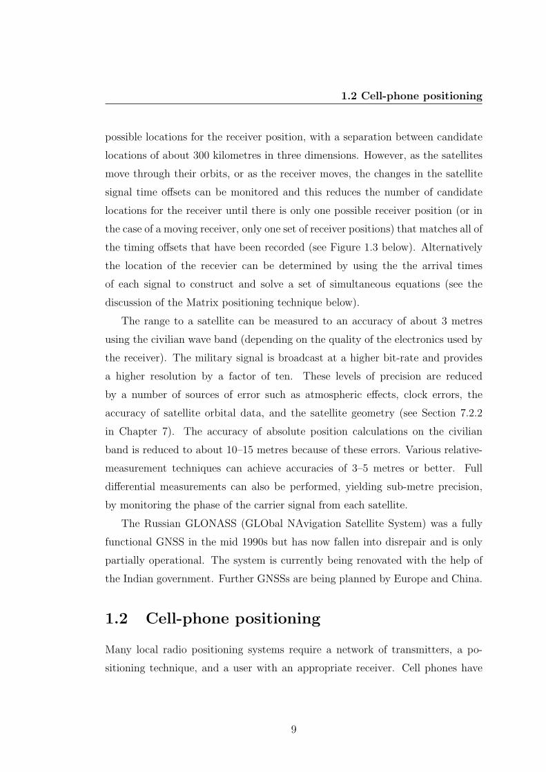
possible locations for the receiver position, with a separation between candidate
locations of about 300 kilometres in three dimensions. However, as the satellites
move through their orbits, or as the receiver moves, the changes in the satellite
signal time offsets can be monitored and this reduces the number of candidate
locations for the receiver until there is only one possible receiver position (or in
the case of a moving receiver, only one set of receiver positions) that matches all of
the timing offsets that have been recorded (see Figure 1.3 below). Alternatively
the location of the recevier can be determined by using the the arrival times
of each signal to construct and solve a set of simultaneous equations (see the
discussion of the Matrix positioning technique below).
The range to a satellite can be measured to an accuracy of about 3 metres
using the civilian wave band (depending on the quality of the electronics used by
the receiver). The military signal is broadcast at a higher bit-rate and provides
a higher resolution by a factor of ten. These levels of precision are reduced
by a number of sources of error such as atmospheric effects, clock errors, the
accuracy of satellite orbital data, and the satellite geometry (see Section 7.2.2
in Chapter 7). The accuracy of absolute position calculations on the civilian
band is reduced to about 10–15 metres because of these errors. Various relative-
measurement techniques can achieve accuracies of 3–5 metres or better. Full
differential measurements can also be performed, yielding sub-metre precision,
by monitoring the phase of the carrier signal from each satellite.
The Russian GLONASS (GLObal NAvigation Satellite System) was a fully
functional GNSS in the mid 1990s but has now fallen into disrepair and is only
partially operational. The system is currently being renovated with the help of
the Indian government. Further GNSSs are being planned by Europe and China.
1.2 Cell-phone positioning
Many local radio positioning systems require a network of transmitters, a po-
sitioning technique, and a user with an appropriate receiver. Cell phones have
9
1. INTRODUCTION TO RADIO POSITIONING
Figure 1.3: Plot showing the variation in candidate locations for a GPS receiver po-sition using the weak-signal method as the satellites move through their orbits. Thegreen markers represent an initial set of candidate locations, the red markers representthe set of candidate locations a few tens of seconds later as the satellites have movedthrough their orbits. As time passes, only one candidate location will be common to allsets for a stationary receiver, and this gives the receiver’s position.
become very popular portable radio receivers, with an estimated 2.5 billion hand-
sets in use the world as of 2006 [6], and so the idea of providing a radio positioning
system via cell phone networks is very attractive. A cell-phone positioning sys-
tem would allow networks and handset manufacturers to provide location-based
services, navigational aid, and the position of a user during an emergency call.
10
1.2 Cell-phone positioning
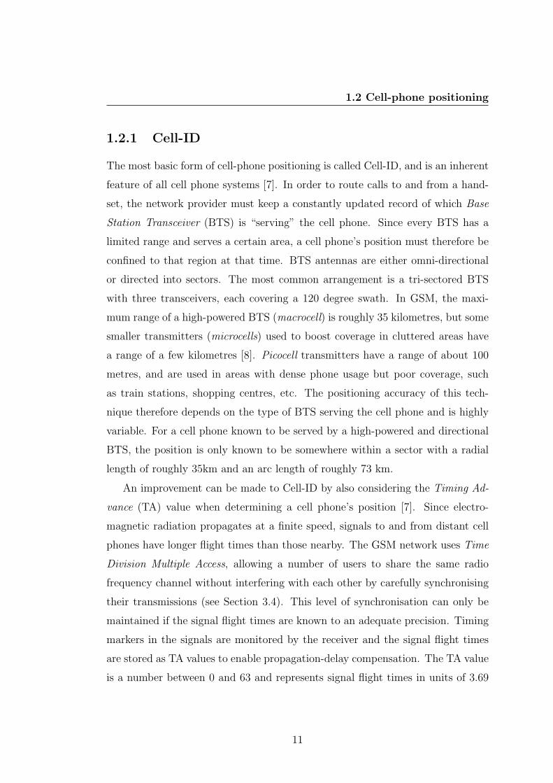
1.2.1 Cell-ID
The most basic form of cell-phone positioning is called Cell-ID, and is an inherent
feature of all cell phone systems [7]. In order to route calls to and from a hand-
set, the network provider must keep a constantly updated record of which Base
Station Transceiver (BTS) is “serving” the cell phone. Since every BTS has a
limited range and serves a certain area, a cell phone’s position must therefore be
confined to that region at that time. BTS antennas are either omni-directional
or directed into sectors. The most common arrangement is a tri-sectored BTS
with three transceivers, each covering a 120 degree swath. In GSM, the maxi-
mum range of a high-powered BTS (macrocell) is roughly 35 kilometres, but some
smaller transmitters (microcells) used to boost coverage in cluttered areas have
a range of a few kilometres [8]. Picocell transmitters have a range of about 100
metres, and are used in areas with dense phone usage but poor coverage, such
as train stations, shopping centres, etc. The positioning accuracy of this tech-
nique therefore depends on the type of BTS serving the cell phone and is highly
variable. For a cell phone known to be served by a high-powered and directional
BTS, the position is only known to be somewhere within a sector with a radial
length of roughly 35km and an arc length of roughly 73 km.
An improvement can be made to Cell-ID by also considering the Timing Ad-
vance (TA) value when determining a cell phone’s position [7]. Since electro-
magnetic radiation propagates at a finite speed, signals to and from distant cell
phones have longer flight times than those nearby. The GSM network uses Time
Division Multiple Access, allowing a number of users to share the same radio
frequency channel without interfering with each other by carefully synchronising
their transmissions (see Section 3.4). This level of synchronisation can only be
maintained if the signal flight times are known to an adequate precision. Timing
markers in the signals are monitored by the receiver and the signal flight times
are stored as TA values to enable propagation-delay compensation. The TA value
is a number between 0 and 63 and represents signal flight times in units of 3.69
11
1. INTRODUCTION TO RADIO POSITIONING
microseconds (the GSM symbol period). This in turn corresponds to increments
of about 1,100 metres in the round-trip signal propagation path. The TA value
therefore increments for every 550 metre change in range between a mobile and
BTS and allows propagation-delay compensation for handsets up to about 35.2
kilometres away. Since the TA value only represents the radial distance from the
BTS the improvement to the positioning accuracy only applies to this aspect of
the cell phone’s position. The position estimate provided by TA with a direc-
tional high powered BTS antenna is an arc in space 550 metres wide which can
be between a few hundred metres and 73 kilometres long depending on the cell
phone’s distance from the BTS.
A further improvement to this technique can be made by forcing the cell
phone to register with other base stations within range and repeating the TA
measurements. Depending on the geometry and number of available base stations,
this can improve the positioning accuracy to around ±275 metres in all directions.
1.2.2 Database Correlation
A technique called the Database Correlation Method (DCM) can also be used to
position cell phones [9]. This system relies on the assumption that each position
in a given region has a unique ‘signal fingerprint’ defined by the set of signal
strength measurements from all nearby BTSs. A database containing the signal
strengths measured at every position in an area is first created either by surveying
or by computer simulation. The handset can then compare a given set of BTS
signal strengths to the values in this database and look up the corresponding
location. Accuracies of 100 metres or better have been demonstrated for outdoor
positioning using a database generated with signal propagation models [9, 10].
Signal propagation models are inadequate for simulating the complicated signal
environments found indoors, but the system has been shown to determine indoor
receiver positions to an accuracy of 5 metres or better using a database generated
12
1.2 Cell-phone positioning
with previously recorded data [11]. However, the signal strength at a given loca-
tion can vary due to changes in the local environment, atmospheric conditions,
and variations in the output from the BTS. A given ‘fingerprint’ is therefore not
necessarily constant and reliable over time.
1.2.3 Enhanced Observed Time Difference
The TDOA technique discussed above can be also be applied to cell phone posi-
tioning, however, the TDOA technique relies on synchronised base station trans-
missions, which are not a feature of the GSM network. This can be accounted
for in a central processing node called a Serving Mobile Location Centre (SMLC),
which constantly monitors the relative transmission times of the BTSs on the
network using measurements made by Location Measurement Units (LMUs) dis-
tributed throughout the network at known locations. The time offsets of the
BTS broadcasts are then taken into account during the TDOA calculations when
positioning a given handset (using the same timing marker used for TA). This
method is called Enhanced Observed Time Difference (E-OTD). The positioning
accuracy depends on the distribution of the BTSs, the use of interpolation tech-
niques (see Section 3.3.1 in Chapter 3), and signal degradation caused by noise
and multipath, but is typically quoted as being in the range of 50–150m [12].
1.2.4 Matrix
The Matrix positioning system, invented and developed by Cambridge Positioning
Systems, is a technique that provides the high accuracy associated with E-OTD
without requiring any LMUs distributed throughout the network [13, 14, 15].
Matrix calculates receiver positions by constructing, and then solving, a set of
simultaneous equations of the form
ctij = |ri − bj|+ εi + αj, (1.2)
13
1. INTRODUCTION TO RADIO POSITIONING
where c is the speed of the radio waves, the vector ri is the position of the
ith receiver, and the vector bj is the position of the jth BTS. The value of tij
represents the arrival time of the timing marker from the jth BTS at the ith
receiver. The ε value is the timing offset of a given receiver and the α value is the
timing offset of a given BTS. The values of t, ε and α are all expressed relative
to an imaginary universal uniform clock.
The set of simultaneous equations cannot be solved for a single stationary
handset, but for a distribution of handsets sharing information, or a single moving
handset, enough data can be gathered to solve the set of equations. For a system
with ‘M ’ receivers and ‘B’ BTSs, the set can be solved when M×B ≥ 3M+B−1.
As more receivers join the distribution, or as any of the current set move, the
extra data continues to be used to improve the accuracy of previous and current
positions by improving the estimates of the ε and α values. Consequently, the
accuracy of the entire track of a single moving cell phone can improve steadily
as the cell phone (or others around it) move around the network. The typical
accuracy of the Matrix method is in the range of 50–150 metres.
1.2.5 Enhanced GPS
E-GPS is a cell phone positioning technique pioneered by Cambridge Positioning
Systems that incorporates both the Matrix system and an integrated, low-power
and low-cost GPS receiver [16]. In E-GPS, the GPS receiver is aided in acquiring
the satellite signals rapidly. In principle, a GPS device could acquire a satellite’s
signal immediately if it had knowledge of both the expected time offset and
frequency offset. The broadcast frequencies appear to be shifted because of the
Doppler effect as the satellites move through their orbits, and the time offsets
of the transmissions depend on the unknown distances to the satellites and the
unknown current value of GPS time. An unassisted GPS device therefore needs
to scan through a large range of frequency and time offsets searching for signals.
This two-dimensional search consists of cross-correlating a known code sequence
14
1.2 Cell-phone positioning
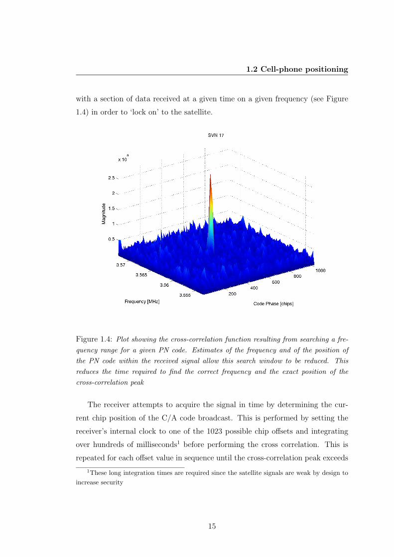
with a section of data received at a given time on a given frequency (see Figure
1.4) in order to ‘lock on’ to the satellite.
Figure 1.4: Plot showing the cross-correlation function resulting from searching a fre-quency range for a given PN code. Estimates of the frequency and of the position ofthe PN code within the received signal allow this search window to be reduced. Thisreduces the time required to find the correct frequency and the exact position of thecross-correlation peak
The receiver attempts to acquire the signal in time by determining the cur-
rent chip position of the C/A code broadcast. This is performed by setting the
receiver’s internal clock to one of the 1023 possible chip offsets and integrating
over hundreds of milliseconds1 before performing the cross correlation. This is
repeated for each offset value in sequence until the cross-correlation peak exceeds
1These long integration times are required since the satellite signals are weak by design toincrease security
15
1. INTRODUCTION TO RADIO POSITIONING
a given threshold, indicating that the signal has been found. If all of the possible
offset values are exhausted before a signal is found, then another frequency must
be searched. Since the C/A code repeats every millisecond, the minimum coher-
ent integration time is a millisecond and therefore the coarsest frequency steps
that a receiver can make during an initial acquisition stage is 1 kHz without risk-
ing ‘missing’ the signal. The combination of the maximum possible Doppler shift
and the possible error on the receiver’s frequency reference results in a total fre-
quency error of up to about ±10 kHz, meaning that there are about 10 frequency
channels to test.
The search time can be reduced by increasing the number of correlators in the
device to allow parallel searching, but this increases its cost. If the GPS device
can estimate the time offset and frequency offset, the signal acquisition time and
required number of correlators can both be greatly reduced. These estimates
can be made using data from a recent position fix by the GPS device itself, or
using data from an external source. This ‘assistance’ data usually includes the
satellite orbital data, an estimate of the GPS receiver location, and an estimate
of the current GPS time. The GPS device can use these pieces of information
to calculate a narrow range of frequency offsets over which to search for each
satellite. The search window is also reduced by estimating the time offsets (i.e.
the code-phase offsets of the PN code sequences in each satellite broadcast) so
that the cross correlations can be performed over smaller time-offset ranges (see
Figure 1.5 below).
GPS devices can perform ‘hot’, ‘warm’, ‘cold’ and ‘autonomous’ starts de-
pending on the accuracy and content of the assistance data they are given or the
amount of time that has passed since their last satellite acquisition. The Time To
First Fix (TTFF) for each of these conditions varies considerably. TTFF refers
to the time taken for a GPS device to return a position calculation after it has
been requested.
16
1.2 Cell-phone positioning
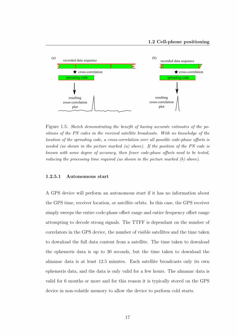
Figure 1.5: Sketch demonstrating the benefit of having accurate estimates of the po-sitions of the PN codes in the received satellite broadcasts. With no knowledge of thelocation of the spreading code, a cross-correlation over all possible code-phase offsets isneeded (as shown in the picture marked (a) above). If the position of the PN code isknown with some degree of accuracy, then fewer code-phase offsets need to be tested,reducing the processing time required (as shown in the picture marked (b) above).
1.2.5.1 Autonomous start
A GPS device will perform an autonomous start if it has no information about
the GPS time, receiver location, or satellite orbits. In this case, the GPS receiver
simply sweeps the entire code-phase offset range and entire frequency offset range
attempting to decode strong signals. The TTFF is dependant on the number of
correlators in the GPS device, the number of visible satellites and the time taken
to download the full data content from a satellite. The time taken to download
the ephemeris data is up to 30 seconds, but the time taken to download the
almanac data is at least 12.5 minutes. Each satellite broadcasts only its own
ephemeris data, and the data is only valid for a few hours. The almanac data is
valid for 6 months or more and for this reason it is typically stored on the GPS
device in non-volatile memory to allow the device to perform cold starts.
17
1. INTRODUCTION TO RADIO POSITIONING
1.2.5.2 Cold start
A GPS device performs a cold start if it only has valid almanac data available.
The TTFF then depends on the time required for the GPS device to acquire
each satellite and then download its ephemeris data. The TTFF is therefore
governed by the number of correlators, the number of available satellites, their
signal strengths and the ephemeris download times. A cold start usually takes at
least 30 seconds.
1.2.5.3 Warm and hot starts
Warm and hot starts are possible if the GPS receiver has the almanac data, valid
ephemeris data for one or more satellites, an estimate of the receiver location
(within 100km or better) and an estimate of GPS time (within a few microseconds
or better). Depending on the accuracy of these estimates and the age of the
ephemeris data, the TTFF range is about 1–15 seconds. A hot start refers to a
TTFF of a few seconds or less.
1.2.5.4 Fine Time Aiding
As discussed above, a GPS device can either store data in order to perform future
warm or hot starts, or be provided with the data from an external source when
required. The device would need to search for (and acquire) satellites every few
hours in order to maintain warm starts independently, which would result in an
unwanted drain of its power supply. This approach would also rely on the device
being in a suitable environment at each ‘update time’ in order to receive the
signals. If the data is provided externally however, then the GPS device only
needs to be powered when a position calculation is required by the user. Every
fix can be then be a warm or hot fix with a low TTFF value, even for a GPS
device which has never been used before.
Assistance data can be categorised into an estimate of the receiver’s position,
an estimate of GPS time, the satellite orbital information, and estimates of the
18
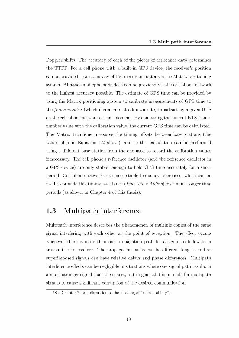
1.3 Multipath interference
Doppler shifts. The accuracy of each of the pieces of assistance data determines
the TTFF. For a cell phone with a built-in GPS device, the receiver’s position
can be provided to an accuracy of 150 metres or better via the Matrix positioning
system. Almanac and ephemeris data can be provided via the cell phone network
to the highest accuracy possible. The estimate of GPS time can be provided by
using the Matrix positioning system to calibrate measurements of GPS time to
the frame number (which increments at a known rate) broadcast by a given BTS
on the cell-phone network at that moment. By comparing the current BTS frame-
number value with the calibration value, the current GPS time can be calculated.
The Matrix technique measures the timing offsets between base stations (the
values of α in Equation 1.2 above), and so this calculation can be performed
using a different base station from the one used to record the calibration values
if necessary. The cell phone’s reference oscillator (and the reference oscillator in
a GPS device) are only stable1 enough to hold GPS time accurately for a short
period. Cell-phone networks use more stable frequency references, which can be
used to provide this timing assistance (Fine Time Aiding) over much longer time
periods (as shown in Chapter 4 of this thesis).
1.3 Multipath interference
Multipath interference describes the phenomenon of multiple copies of the same
signal interfering with each other at the point of reception. The effect occurs
whenever there is more than one propagation path for a signal to follow from
transmitter to receiver. The propagation paths can be different lengths and so
superimposed signals can have relative delays and phase differences. Multipath
interference effects can be negligible in situations where one signal path results in
a much stronger signal than the others, but in general it is possible for multipath
signals to cause significant corruption of the desired communication.
1See Chapter 2 for a discussion of the meaning of “clock stability”.
19
1. INTRODUCTION TO RADIO POSITIONING
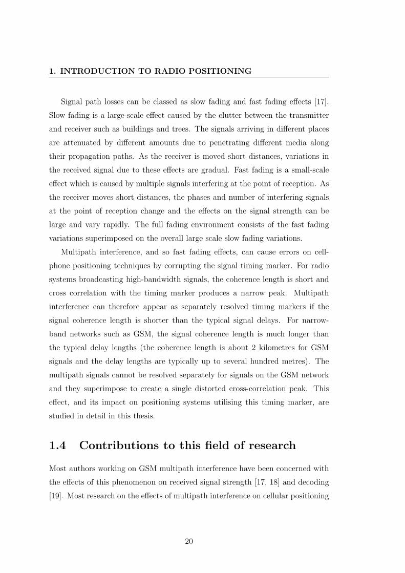
Signal path losses can be classed as slow fading and fast fading effects [17].
Slow fading is a large-scale effect caused by the clutter between the transmitter
and receiver such as buildings and trees. The signals arriving in different places
are attenuated by different amounts due to penetrating different media along
their propagation paths. As the receiver is moved short distances, variations in
the received signal due to these effects are gradual. Fast fading is a small-scale
effect which is caused by multiple signals interfering at the point of reception. As
the receiver moves short distances, the phases and number of interfering signals
at the point of reception change and the effects on the signal strength can be
large and vary rapidly. The full fading environment consists of the fast fading
variations superimposed on the overall large scale slow fading variations.
Multipath interference, and so fast fading effects, can cause errors on cell-
phone positioning techniques by corrupting the signal timing marker. For radio
systems broadcasting high-bandwidth signals, the coherence length is short and
cross correlation with the timing marker produces a narrow peak. Multipath
interference can therefore appear as separately resolved timing markers if the
signal coherence length is shorter than the typical signal delays. For narrow-
band networks such as GSM, the signal coherence length is much longer than
the typical delay lengths (the coherence length is about 2 kilometres for GSM
signals and the delay lengths are typically up to several hundred metres). The
multipath signals cannot be resolved separately for signals on the GSM network
and they superimpose to create a single distorted cross-correlation peak. This
effect, and its impact on positioning systems utilising this timing marker, are
studied in detail in this thesis.
1.4 Contributions to this field of research
Most authors working on GSM multipath interference have been concerned with
the effects of this phenomenon on received signal strength [17, 18] and decoding
[19]. Most research on the effects of multipath interference on cellular positioning
20
1.5 Thesis outline
systems has previously involved either (a) ray-tracing computer simulations [20],
or (b) studying a radio signal created specifically for the research, which cannot
be broadcast in the cellular frequency bands and is not structured in the same
way as the cell phone signals [21]. Some research has been performed using real
cellular signals to produce empirical models of the effects of multipath interference
on positioning systems [22].
The work I present here consists of accurate and high-resolution measurements
of the GSM signals using an atomic reference, the first absolute measurements
of signal flight times on GSM networks, models that reproduce the observed
multipath interference effects, and two new methods of determining GSM signal
arrival times which remove the largest errors caused by multipath interference.
1.5 Thesis outline
Chapter 1 - Introduction to radio positioning
This chapter provides a summary of local radio positioning techniques and their
history. A discussion of radio positioning techniques specific to the GSM network
is included, followed by a description of multipath interference, signal fading, and
the content of this thesis.
Chapter 2 - Timing stability
This chapter describes the importance of timing stability to the experimental
stages of the project and discusses various frequency references. The concept of
Allan variance as a measure of timing stability is included. An experiment was
performed to determine the timing error associated with the experimental appa-
ratus used for this research and the results are presented here.
Chapter 3 - Time of flight measurements on cellular networks
This chapter presents two methods for measuring signal arrival times on the GSM
network along with a discussion of the apparatus and experimental techniques
21
1. INTRODUCTION TO RADIO POSITIONING
used during the research presented in this thesis.
Chapter 4 - GSM network stability
This chapter presents the results of a series of experiments which measured the
temporal stabilities of a number of cell phone base stations from two different
network providers at a stationary receiver.
Chapter 5 - Effects of indoor multipath environments on GSM tim-
ing stability
This chapter presents the results of a series of experiments which measured the
degradation of the apparent temporal stability of received signals on the GSM
network caused by moving a receiver slowly over sub-wavelength distances in-
doors.
Chapter 6 - Modelling the effects of indoor multipath environments
on GSM timing stability
A model based on multipath interference is presented and shown to reproduce
the behaviour observed in the experiments described in Chapter 5.
Chapter 7 - A study of the timing errors encountered when performing
radio location using the GSM network
This chapter presents the results of a series of experiments which measured the
distributions of the errors on signal arrival times in various environments. A
model based on multipath interference is proposed and is shown to reproduce the
experimentally-obtained distributions.
Chapter 8 - Summary and further work
This chapter presents a summary of the results obtained from the work carried
out in this thesis and suggests further work.
22
Chapter 2
Timing stability
The aim of the research described in this thesis was to study the effects of multi-
path interference in various environments on the apparent arrival times of signals
radiated by GSM base stations. There were four main stages in this investigation:
a) designing and building a set of apparatus to gather data;
b) determining the signal stabilities of the base station transmissions;
c) determining the signal stabilities on reception in varying environments; and
d) modelling the signal stabilities.
There were three limiting aspects to making timing measurements. The first was
the resolution with which any measurement was made. The signals being mea-
sured were continuous but the apparatus sampled the signals at discrete instances
with a fixed sampling period. Fluctuations on time scales shorter than twice this
period were not resolved and contributed only to noise.
The second was the accuracy with which each measurement was made. The
effect of the quantisation of the analogue measurements by the digital apparatus
is considered in the next chapter. Here, the calibration of the reference oscillator
against which the measurements were compared is considered. In this sense, the
accuracy of the frequency reference is defined as the difference between its output
frequency averaged over a given time interval and its nominal frequency.
23
2. TIMING STABILITY
The third limiting aspect was the frequency stability of the reference oscillator.
Frequency stability refers to the repeatability of frequency measurements and is
determined by the distribution of error around the average value for a given set
of measurements. An oscillator can be stable but not accurate and it can be
accurate but not stable (i.e. stability and accuracy are independent attributes).
These lead to the concepts of frequency bias error and frequency bias rate error
(see Figure 2.1 below). The instantaneous frequency ω of an oscillator can be
modelled using a power series expansion,
ω = ω0 + ω′t+ ω′′t2 + ... (2.1)
where ω0 is the frequency at t = 0, ω′ is the first-order frequency variation with
time, ω′′ is the second order frequency variation with time, etc. The frequency
bias error is given by ∆ωb = ω0 − ωn, where ωn is the nominal frequency. The
frequency bias rate error is given by ω′. The higher order terms are not usually
named. The instantaneous frequency error is given by
∆ω(t) = ω0 − ωn + ω′t+ ω′′t2 + ... (2.2)
2.1 Allan Variance
The stability of a test oscillator can be determined by analysing its phase fluc-
tuations when compared to a reference oscillator [23]. A perfect oscillator would
produce a pure sine wave,
V (t) = V0 cos (2πf0t) , (2.3)
but in reality there is always some phase noise associated with the output signal.
A more realistic model is therefore given by
V (t) = V0 cos [2πf0t+ φ (t)] , (2.4)
24
2.1 Allan Variance
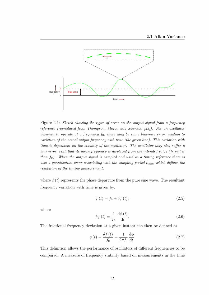
Figure 2.1: Sketch showing the types of error on the output signal from a frequencyreference (reproduced from Thompson, Moran and Swenson [23]). For an oscillatordesigned to operate at a frequency f0, there may be some bias-rate error, leading tovariation of the actual output frequency with time (the green line). This variation withtime is dependent on the stability of the oscillator. The oscillator may also suffer abias error, such that its mean frequency is displaced from the intended value (fb ratherthan f0). When the output signal is sampled and used as a timing reference there isalso a quantisation error associating with the sampling period tmin, which defines theresolution of the timing measurement.
where φ (t) represents the phase departure from the pure sine wave. The resultant
frequency variation with time is given by,
f (t) = f0 + δf (t) , (2.5)
where
δf (t) =1
2π
dφ (t)
dt. (2.6)
The fractional frequency deviation at a given instant can then be defined as
y (t) =δf (t)
f0
=1
2πf0
dφ
dt. (2.7)
This definition allows the performance of oscillators of different frequencies to be
compared. A measure of frequency stability based on measurements in the time
25
2. TIMING STABILITY
domain can be made by considering a set of frequency measurements recorded
with sampling period τ and the average fractional frequency deviation given by
yk =1
τ
∫ tk+τ
tk
y (t) dt. (2.8)
Combining this with equation 2.7 gives
yk =φ (tk + τ)− φ (tk)
2πf0τ. (2.9)
Measurements of yk are made at the repetition interval T , where T ≥ τ and such
that tk+1 = tk +T . The value of φ represents the phase of the test oscillator with
respect to the reference. The values of t and τ are also measured with respect to
the reference oscillator. A measure of the test oscillator’s frequency stability can
then be formed as the sample variance of yk given by
⟨σ2y (N, T, τ)
⟩=
1
N − 1
⟨N∑n=1
(yn −
1
N
N∑k=1
yk
)2⟩, (2.10)
where N is the number of time intervals of length T . As N → ∞ the above
quantity becomes the true variance. In many cases, however, equation 2.10 does
not converge because of the low-frequency behaviour of the power spectrum of
y, and then the true variance is not defined. This occurs because the long term
behaviour of an oscillator is determined by a random walk process and the timing
error at any point is the accumulation of all the past timing errors. This phe-
nomenon results in the true variance being unbounded. To avoid this problem, a
particular case of equation 2.10 is more commonly used with N = 2 and T = τ .
This two-sample variance is referred to as the Allan variance [24] and is given by
σ2A(τ) =
⟨(yk+1 − yk)
2⟩2
, (2.11)
or from equation 2.9,
σ2A(τ) =
⟨[φ (t+ 2τ)− 2φ (t+ τ) + φ (t)]2
⟩8 (πf0τ)
2 . (2.12)
26
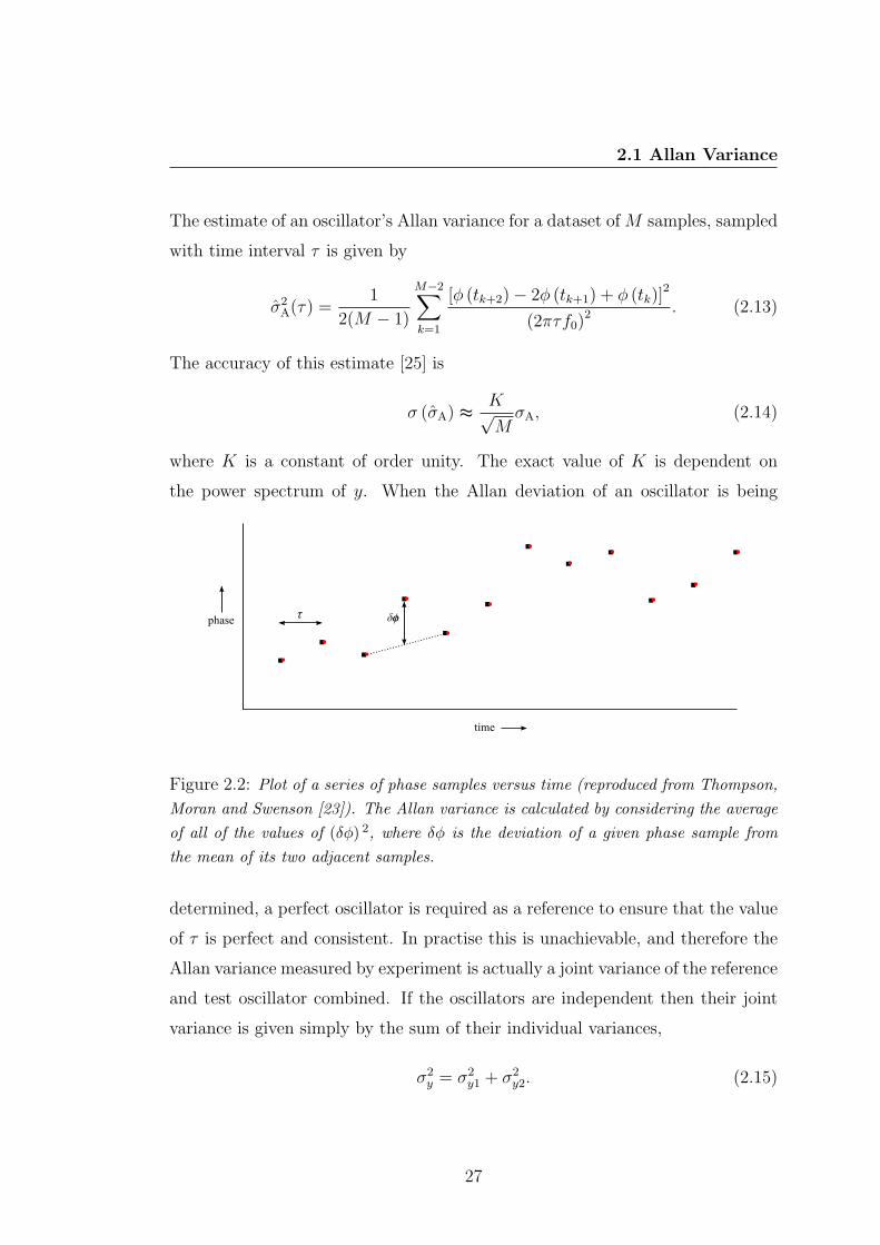
2.1 Allan Variance
The estimate of an oscillator’s Allan variance for a dataset of M samples, sampled
with time interval τ is given by
σ2A(τ) =
1
2(M − 1)
M−2∑k=1
[φ (tk+2)− 2φ (tk+1) + φ (tk)]2
(2πτf0)2 . (2.13)
The accuracy of this estimate [25] is
σ (σA) ≈K√MσA, (2.14)
where K is a constant of order unity. The exact value of K is dependent on
the power spectrum of y. When the Allan deviation of an oscillator is being
Figure 2.2: Plot of a series of phase samples versus time (reproduced from Thompson,Moran and Swenson [23]). The Allan variance is calculated by considering the averageof all of the values of (δφ) 2, where δφ is the deviation of a given phase sample fromthe mean of its two adjacent samples.
determined, a perfect oscillator is required as a reference to ensure that the value
of τ is perfect and consistent. In practise this is unachievable, and therefore the
Allan variance measured by experiment is actually a joint variance of the reference
and test oscillator combined. If the oscillators are independent then their joint
variance is given simply by the sum of their individual variances,
σ2y = σ2
y1 + σ2y2. (2.15)
27
2. TIMING STABILITY
Three approaches can be used to determine a test oscillator’s Allan variance. If
the test oscillator is known to be much less stable than the reference oscillator
(such that σ2y1 σ2
y2), then the joint variance will be a close estimate of the test
oscillator’s variance. Alternatively, if an oscillator similar to the test oscillator can
be used for the reference (σ2y1 ≈ σ2
y2), then the Allan variance of the test oscillator
can be estimated as half of the measured Allan variance. In reality, however, two
oscillators of the same design will not be identical, and so an alternative estimate
is given by comparing three oscillators simultaneously. The three joint variances
are given by σ2ij, σ
2jk and σ2
ik where the individual variances are σ2i , σ
2j and σ2
k. Each
individual variance can then be calculated using the following set of equations
[26],
σ2i =
1
2
(σ2ij + σ2
ik − σ2jk
), (2.16)
σ2j =
1
2
(σ2jk + σ2
ij − σ2ik
), (2.17)
σ2k =
1
2
(σ2jk + σ2
ik − σ2ij
). (2.18)
For calculations of the Allan variance at time periods approaching half the length
of the experiment it is possible to find a negative sample Allan variance using this
approach. This occurs because of the lack of data for that time period resulting
in significant errors on the values of the joint variances (see equation 2.14 above).
Allan variances cannot be negative by their definition and so caution must be
exercised for long time periods with few data points.
Allan deviation plots of the logarithm of σA(τ) versus the logarithm of τ
are useful in analysing the stability of a test oscillator and are more conven-
tional in the literature than Allan variance plots. Allan deviation plots often
exhibit behaviour which can be categorised into four regimes as shown in Fig-
ure 2.3 below. These regimes are determined by a number of different processes
[27, 28], and are separable because of the distinct power-law dependencies of these
processes. Noise with a flat power spectrum independent of frequency is called
28
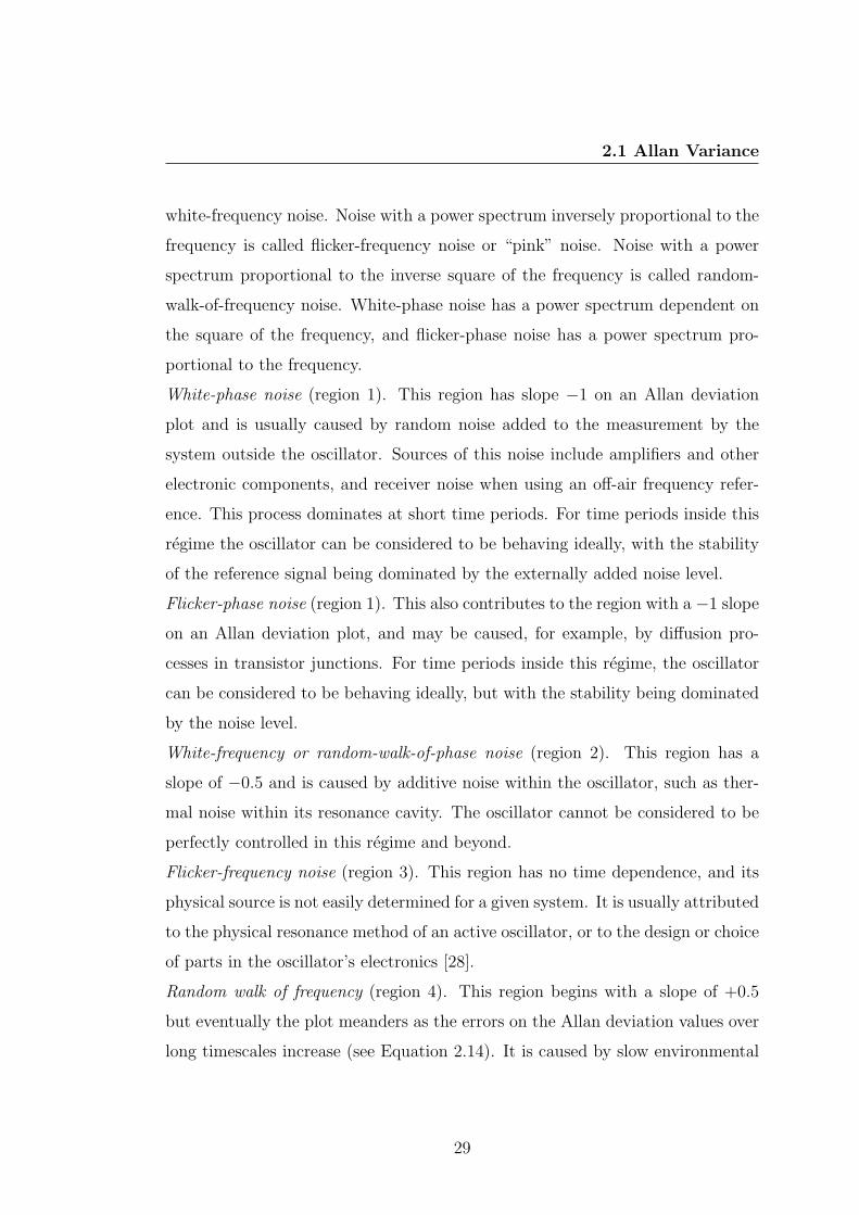
2.1 Allan Variance
white-frequency noise. Noise with a power spectrum inversely proportional to the
frequency is called flicker-frequency noise or “pink” noise. Noise with a power
spectrum proportional to the inverse square of the frequency is called random-
walk-of-frequency noise. White-phase noise has a power spectrum dependent on
the square of the frequency, and flicker-phase noise has a power spectrum pro-
portional to the frequency.
White-phase noise (region 1). This region has slope −1 on an Allan deviation
plot and is usually caused by random noise added to the measurement by the
system outside the oscillator. Sources of this noise include amplifiers and other
electronic components, and receiver noise when using an off-air frequency refer-
ence. This process dominates at short time periods. For time periods inside this
regime the oscillator can be considered to be behaving ideally, with the stability
of the reference signal being dominated by the externally added noise level.
Flicker-phase noise (region 1). This also contributes to the region with a −1 slope
on an Allan deviation plot, and may be caused, for example, by diffusion pro-
cesses in transistor junctions. For time periods inside this regime, the oscillator
can be considered to be behaving ideally, but with the stability being dominated
by the noise level.
White-frequency or random-walk-of-phase noise (region 2). This region has a
slope of −0.5 and is caused by additive noise within the oscillator, such as ther-
mal noise within its resonance cavity. The oscillator cannot be considered to be
perfectly controlled in this regime and beyond.
Flicker-frequency noise (region 3). This region has no time dependence, and its
physical source is not easily determined for a given system. It is usually attributed
to the physical resonance method of an active oscillator, or to the design or choice
of parts in the oscillator’s electronics [28].
Random walk of frequency (region 4). This region begins with a slope of +0.5
but eventually the plot meanders as the errors on the Allan deviation values over
long timescales increase (see Equation 2.14). It is caused by slow environmental
29
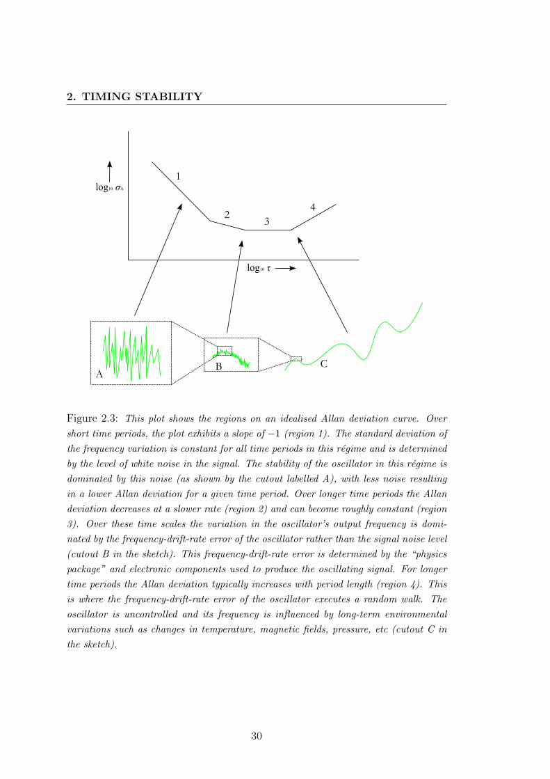
2. TIMING STABILITY
Figure 2.3: This plot shows the regions on an idealised Allan deviation curve. Overshort time periods, the plot exhibits a slope of −1 (region 1). The standard deviation ofthe frequency variation is constant for all time periods in this regime and is determinedby the level of white noise in the signal. The stability of the oscillator in this regime isdominated by this noise (as shown by the cutout labelled A), with less noise resultingin a lower Allan deviation for a given time period. Over longer time periods the Allandeviation decreases at a slower rate (region 2) and can become roughly constant (region3). Over these time scales the variation in the oscillator’s output frequency is domi-nated by the frequency-drift-rate error of the oscillator rather than the signal noise level(cutout B in the sketch). This frequency-drift-rate error is determined by the “physicspackage” and electronic components used to produce the oscillating signal. For longertime periods the Allan deviation typically increases with period length (region 4). Thisis where the frequency-drift-rate error of the oscillator executes a random walk. Theoscillator is uncontrolled and its frequency is influenced by long-term environmentalvariations such as changes in temperature, magnetic fields, pressure, etc (cutout C inthe sketch).
30
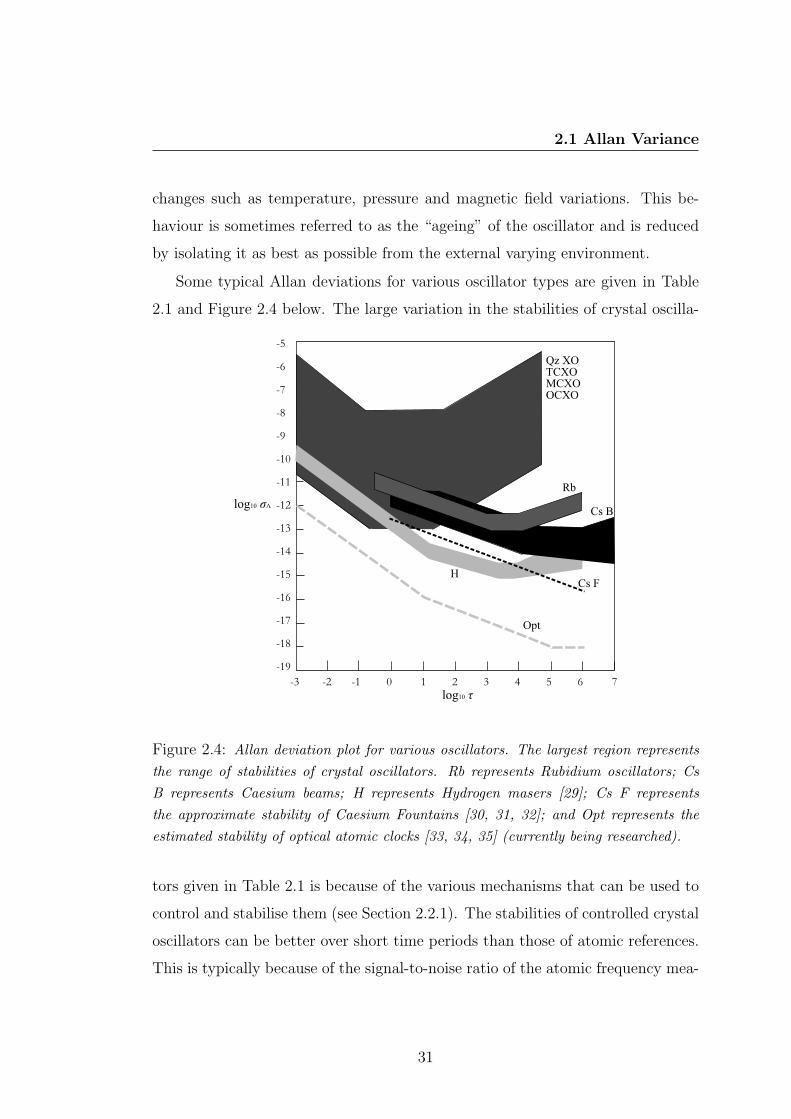
2.1 Allan Variance
changes such as temperature, pressure and magnetic field variations. This be-
haviour is sometimes referred to as the “ageing” of the oscillator and is reduced
by isolating it as best as possible from the external varying environment.
Some typical Allan deviations for various oscillator types are given in Table
2.1 and Figure 2.4 below. The large variation in the stabilities of crystal oscilla-
Figure 2.4: Allan deviation plot for various oscillators. The largest region representsthe range of stabilities of crystal oscillators. Rb represents Rubidium oscillators; CsB represents Caesium beams; H represents Hydrogen masers [29]; Cs F representsthe approximate stability of Caesium Fountains [30, 31, 32]; and Opt represents theestimated stability of optical atomic clocks [33, 34, 35] (currently being researched).
tors given in Table 2.1 is because of the various mechanisms that can be used to
control and stabilise them (see Section 2.2.1). The stabilities of controlled crystal
oscillators can be better over short time periods than those of atomic references.
This is typically because of the signal-to-noise ratio of the atomic frequency mea-
31
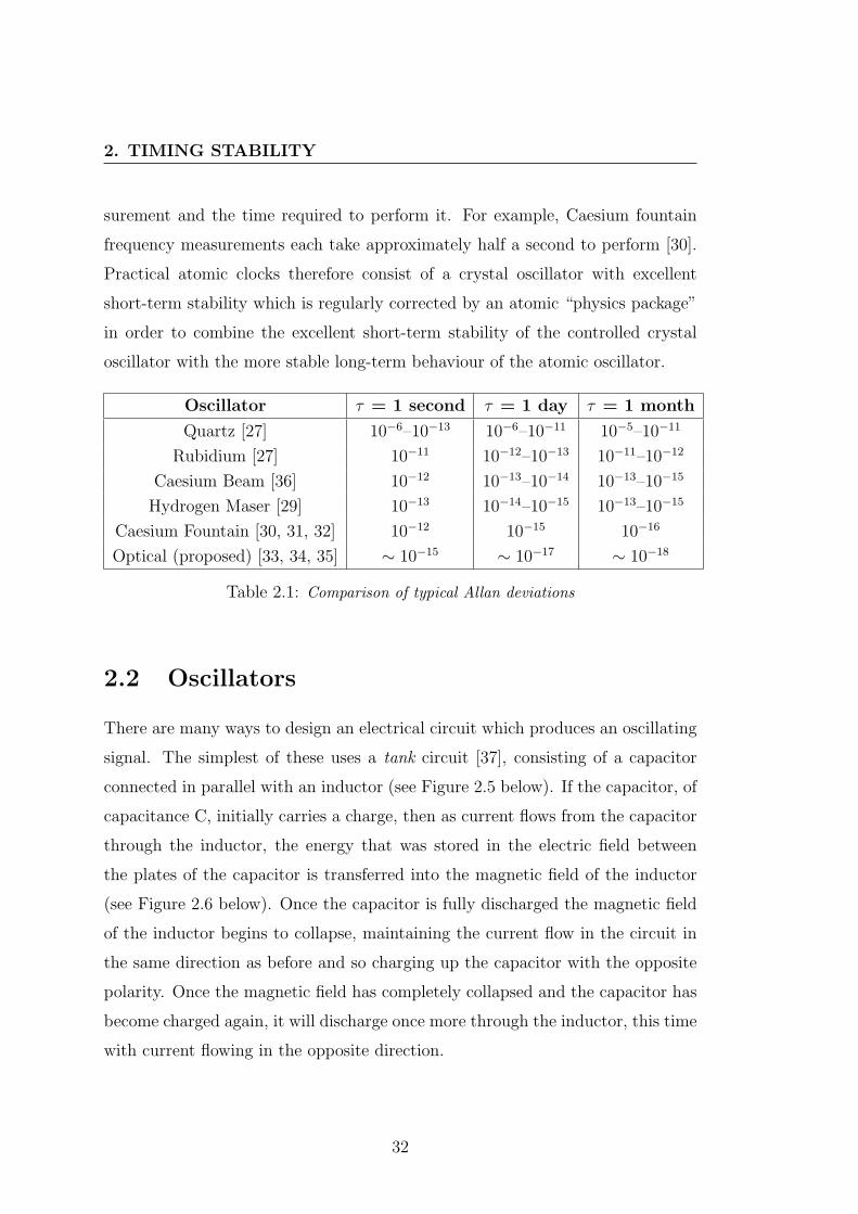
2. TIMING STABILITY
surement and the time required to perform it. For example, Caesium fountain
frequency measurements each take approximately half a second to perform [30].
Practical atomic clocks therefore consist of a crystal oscillator with excellent
short-term stability which is regularly corrected by an atomic “physics package”
in order to combine the excellent short-term stability of the controlled crystal
oscillator with the more stable long-term behaviour of the atomic oscillator.
Oscillator τ = 1 second τ = 1 day τ = 1 month
Quartz [27] 10−6–10−13 10−6–10−11 10−5–10−11
Rubidium [27] 10−11 10−12–10−13 10−11–10−12
Caesium Beam [36] 10−12 10−13–10−14 10−13–10−15
Hydrogen Maser [29] 10−13 10−14–10−15 10−13–10−15
Caesium Fountain [30, 31, 32] 10−12 10−15 10−16
Optical (proposed) [33, 34, 35] ∼ 10−15 ∼ 10−17 ∼ 10−18
Table 2.1: Comparison of typical Allan deviations
2.2 Oscillators
There are many ways to design an electrical circuit which produces an oscillating
signal. The simplest of these uses a tank circuit [37], consisting of a capacitor
connected in parallel with an inductor (see Figure 2.5 below). If the capacitor, of
capacitance C, initially carries a charge, then as current flows from the capacitor
through the inductor, the energy that was stored in the electric field between
the plates of the capacitor is transferred into the magnetic field of the inductor
(see Figure 2.6 below). Once the capacitor is fully discharged the magnetic field
of the inductor begins to collapse, maintaining the current flow in the circuit in
the same direction as before and so charging up the capacitor with the opposite
polarity. Once the magnetic field has completely collapsed and the capacitor has
become charged again, it will discharge once more through the inductor, this time
with current flowing in the opposite direction.
32
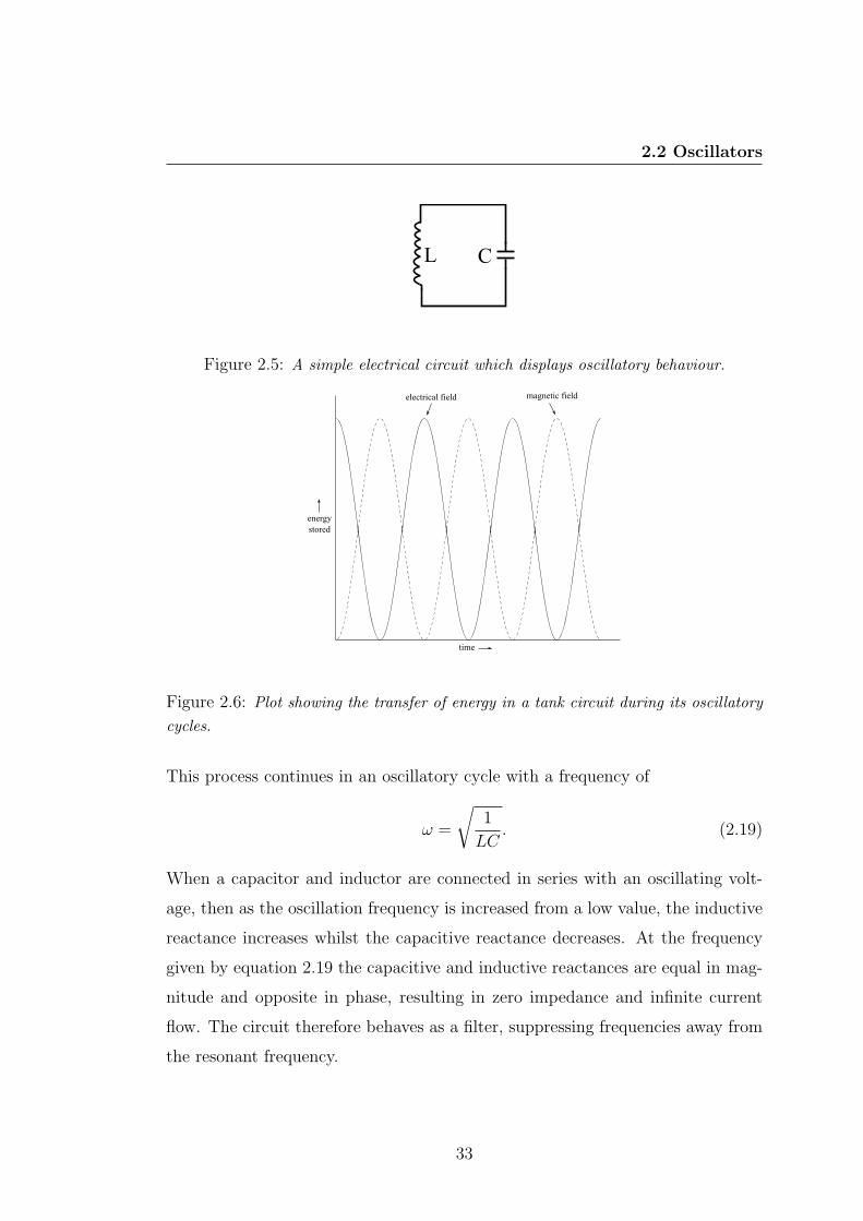
2.2 Oscillators
Figure 2.5: A simple electrical circuit which displays oscillatory behaviour.
Figure 2.6: Plot showing the transfer of energy in a tank circuit during its oscillatorycycles.
This process continues in an oscillatory cycle with a frequency of
ω =
√1
LC. (2.19)
When a capacitor and inductor are connected in series with an oscillating volt-
age, then as the oscillation frequency is increased from a low value, the inductive
reactance increases whilst the capacitive reactance decreases. At the frequency
given by equation 2.19 the capacitive and inductive reactances are equal in mag-
nitude and opposite in phase, resulting in zero impedance and infinite current
flow. The circuit therefore behaves as a filter, suppressing frequencies away from
the resonant frequency.
33
2. TIMING STABILITY
In practise, there is always some resistance in the circuit, which results in
dissipation of the energy. This can be described in terms of the quality factor Q,
defined by
Q = 2π × energy stored
energy lost per cycle. (2.20)
When an oscillatory system is driven at a given frequency, its response is depen-
dant on Q and the driving frequency. As the driving frequency is moved away
from the system’s resonant frequency, the amplitude of driven oscillations for a
high Q system will decrease more rapidly than for a low Q system (see Figure
2.7 below). The width of the resonance peak, defined as the range of frequencies
between the half-power points of the resonance peak, is given by
∆f =f0
Q. (2.21)
The narrower the frequency response of the oscillatory element, the more stable
the oscillator can be. A perfect oscillatory element with an infinite value of Q
could, in theory, be used to make a frequency reference that would have only one
frequency component in its output.
2.2.1 Crystal oscillators
A piezoelectric crystal responds mechanically to an externally applied electric
field, and can also be used to generate a voltage by physically deforming it. This
behaviour allows the crystal to store and release energy, and when placed in an
electrical circuit it is equivalent to the system of electrical components shown
below in Figure 2.8. The section of the circuit with a capacitor, inductor and
resistor in series corresponds to the electrical properties of the vibrating crystal
itself. The capacitance (C0) in parallel with them corresponds to the capacitance
between the electrodes connecting the crystal to the circuit and any stray capac-
itance due to the crystal enclosure. This circuit can oscillate in two ways. The
series section containing C1 and L1 becomes resonant when the impedances of
the capacitor (ZC1 = 1iωC1
) and inductor (ZL1 = iωL1) are equal in magnitude
34
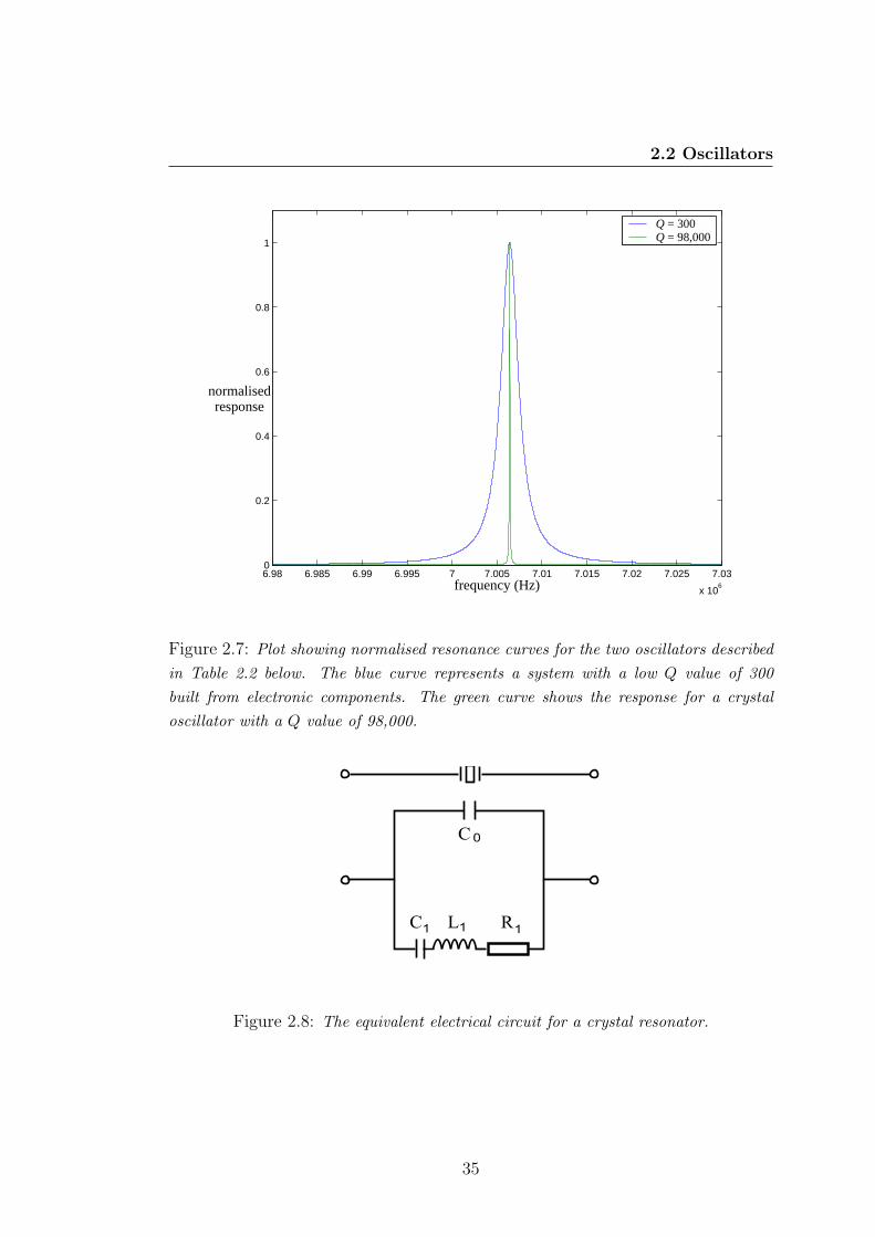
2.2 Oscillators
6.98 6.985 6.99 6.995 7 7.005 7.01 7.015 7.02 7.025 7.03
x 106
0
0.2
0.4
0.6
0.8
1
frequency (Hz)
normalisedresponse
Q = 300 Q = 98,000
Figure 2.7: Plot showing normalised resonance curves for the two oscillators describedin Table 2.2 below. The blue curve represents a system with a low Q value of 300built from electronic components. The green curve shows the response for a crystaloscillator with a Q value of 98,000.
Figure 2.8: The equivalent electrical circuit for a crystal resonator.
35
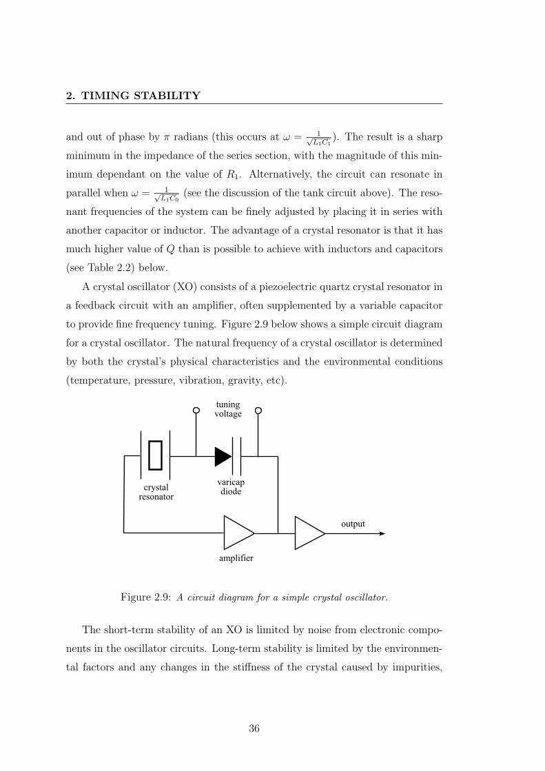
2. TIMING STABILITY
and out of phase by π radians (this occurs at ω = 1√L1C1
). The result is a sharp
minimum in the impedance of the series section, with the magnitude of this min-
imum dependant on the value of R1. Alternatively, the circuit can resonate in
parallel when ω = 1√L1C0
(see the discussion of the tank circuit above). The reso-
nant frequencies of the system can be finely adjusted by placing it in series with
another capacitor or inductor. The advantage of a crystal resonator is that it has
much higher value of Q than is possible to achieve with inductors and capacitors
(see Table 2.2) below.
A crystal oscillator (XO) consists of a piezoelectric quartz crystal resonator in
a feedback circuit with an amplifier, often supplemented by a variable capacitor
to provide fine frequency tuning. Figure 2.9 below shows a simple circuit diagram
for a crystal oscillator. The natural frequency of a crystal oscillator is determined
by both the crystal’s physical characteristics and the environmental conditions
(temperature, pressure, vibration, gravity, etc).
Figure 2.9: A circuit diagram for a simple crystal oscillator.
The short-term stability of an XO is limited by noise from electronic compo-
nents in the oscillator circuits. Long-term stability is limited by the environmen-
tal factors and any changes in the stiffness of the crystal caused by impurities,
36
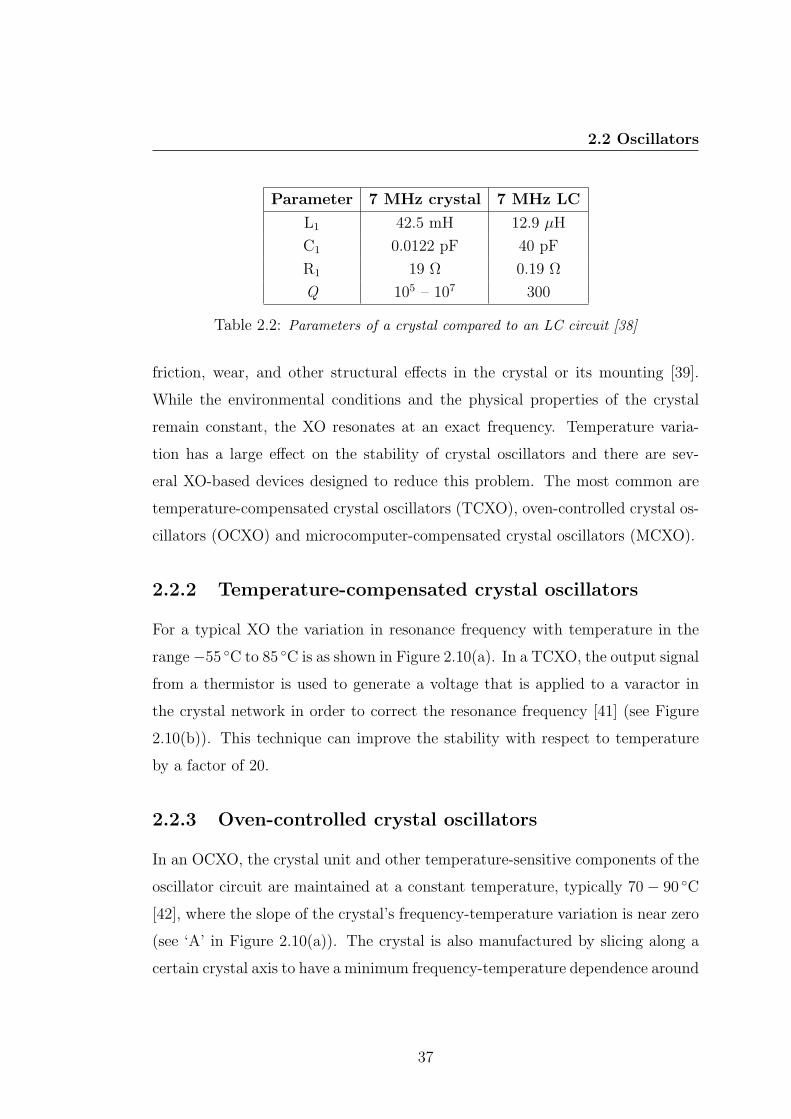
2.2 Oscillators
Parameter 7 MHz crystal 7 MHz LC
L1 42.5 mH 12.9 µH
C1 0.0122 pF 40 pF
R1 19 Ω 0.19 Ω
Q 105 – 107 300
Table 2.2: Parameters of a crystal compared to an LC circuit [38]
friction, wear, and other structural effects in the crystal or its mounting [39].
While the environmental conditions and the physical properties of the crystal
remain constant, the XO resonates at an exact frequency. Temperature varia-
tion has a large effect on the stability of crystal oscillators and there are sev-
eral XO-based devices designed to reduce this problem. The most common are
temperature-compensated crystal oscillators (TCXO), oven-controlled crystal os-
cillators (OCXO) and microcomputer-compensated crystal oscillators (MCXO).
2.2.2 Temperature-compensated crystal oscillators
For a typical XO the variation in resonance frequency with temperature in the
range−55 C to 85 C is as shown in Figure 2.10(a). In a TCXO, the output signal
from a thermistor is used to generate a voltage that is applied to a varactor in
the crystal network in order to correct the resonance frequency [41] (see Figure
2.10(b)). This technique can improve the stability with respect to temperature
by a factor of 20.
2.2.3 Oven-controlled crystal oscillators
In an OCXO, the crystal unit and other temperature-sensitive components of the
oscillator circuit are maintained at a constant temperature, typically 70− 90 C
[42], where the slope of the crystal’s frequency-temperature variation is near zero
(see ‘A’ in Figure 2.10(a)). The crystal is also manufactured by slicing along a
certain crystal axis to have a minimum frequency-temperature dependence around
37
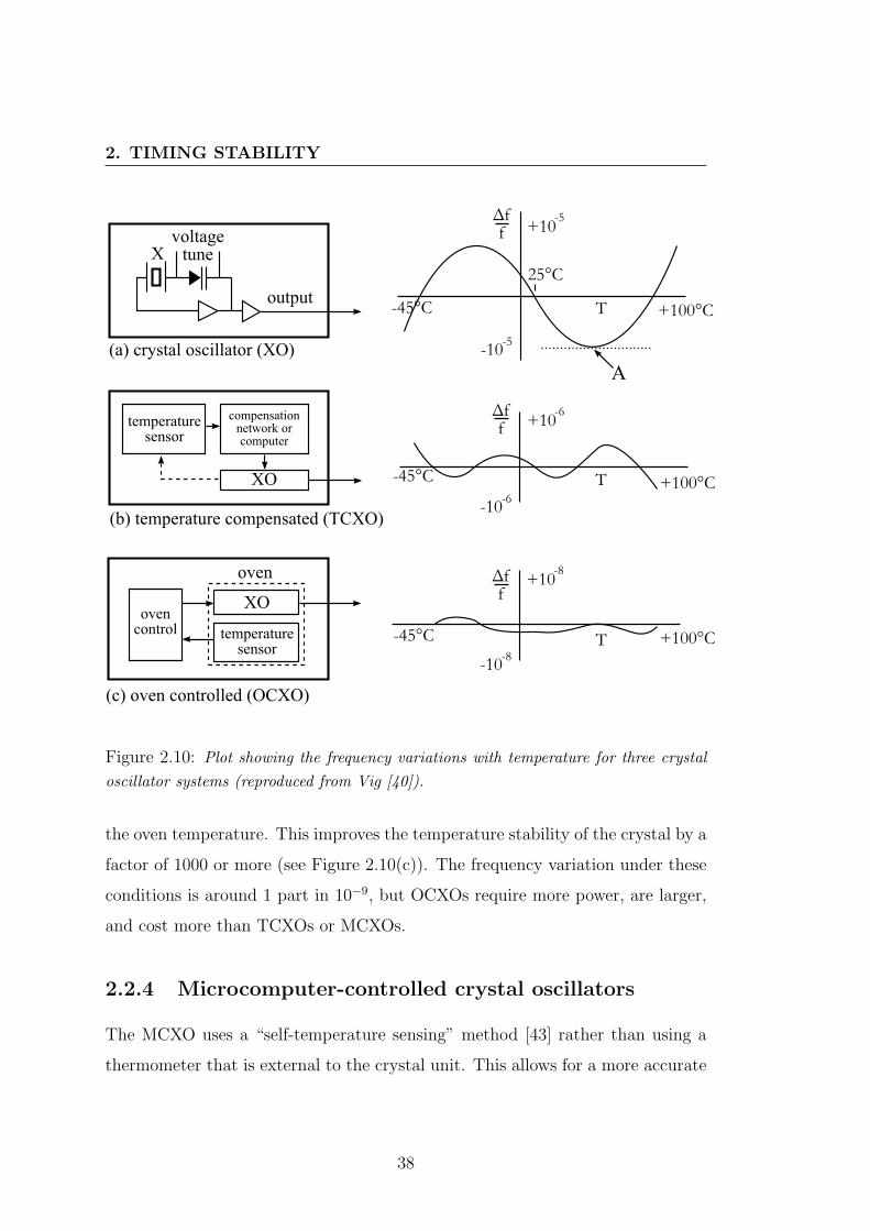
2. TIMING STABILITY
Figure 2.10: Plot showing the frequency variations with temperature for three crystaloscillator systems (reproduced from Vig [40]).
the oven temperature. This improves the temperature stability of the crystal by a
factor of 1000 or more (see Figure 2.10(c)). The frequency variation under these
conditions is around 1 part in 10−9, but OCXOs require more power, are larger,
and cost more than TCXOs or MCXOs.
2.2.4 Microcomputer-controlled crystal oscillators
The MCXO uses a “self-temperature sensing” method [43] rather than using a
thermometer that is external to the crystal unit. This allows for a more accurate
38
2.3 Atomic oscillators
measurement of the temperature of the crystal to be made than in a TCXO. Two
vibrational modes of the crystal are excited simultaneously and are combined such
that the resulting beat frequency is a monotonic (and nearly linear) function of
temperature. The crystal therefore senses its own temperature and a correction
voltage is applied to the varactor. The frequency variation with temperature of
an MCXO in the range −55 C to 85 C is around 1 part in 10−8.
2.3 Atomic oscillators
The principle of an atomic oscillator (also known as an atomic clock) is to use
an atomic resonance frequency as a reference. This can be achieved in two ways.
In an active atomic clock, the photons released during the quantum transition
between two known energy levels can be used directly to provide the reference
frequency. In a passive atomic clock, a feedback circuit is used to match the
frequency of an OCXO or a laser to the transition frequency. In each case, the
reference frequency is provided via photon interaction with a quantum transition
on the atomic scale, and so can be less affected by environmental factors than the
mechanical vibration of a crystal. The two key requirements for a highly-stable
atomic reference are (i) a narrow atomic resonance (corresponding to a high Q
value) and (ii) a high signal-to-noise ratio. Heisenberg’s uncertainty principle
indicates that the narrowest resonance is obtained with the longest interaction
time (∆E∆t & ~ where ∆E = 2π~∆f). The stability of an atomic reference
is therefore typically poorest for very small time periods. In a passive atomic
clock such as the Rubidium standard used in this project, an OCXO provides the
output frequency signal and is continuously corrected to match the frequency of
the atomic absorption resonance, combining the excellent short-term stability of
an OCXO with the excellent long-term stability of an atomic oscillator.
The main types of atomic clocks utilise atomic transitions in Rubidium, Cae-
sium or Hydrogen gases and are discussed briefly below.
39
2. TIMING STABILITY
2.3.1 Rubidium oscillators
Rubidium is an alkali metal with a single valence electron. The spatial distribu-
tion of electrons in an atom depends on their values of n (the principal quantum
number), and l (the orbital angular-momentum quantum number). If an electron
has l 6= 0, then there is also some magnetic moment associated with it. Further-
more, electrons all have an intrinsic magnetic moment, or spin. The interaction
between the orbital magnetic moment and the intrinsic magnetic moment is called
spin-orbit coupling, or LS coupling, and is largely responsible for the complexity
of atomic spectra.
The electronic configuration of the ground state of Rubidium [44] is
1s22s22p63s23p63d104s24p65s.
There are four fully-filled shells (numbers 1− 4) and a single electron in the 5th
shell. The spectroscopic notation uses capital letters and so the electron in the
5s shell has the spectroscopic state given by 52S1/2 [44]. In this convention, the
upright letter S indicates that the total orbital angular momentum of the electron
is zero (l = 0), the upright letters P,D and F correspond to the total orbital
angular momentum quantum numbers 1, 2 and 3 accordingly. The superscript
value in the spectroscopic notation is given by (2S + 1) where italic S is the
total electron spin angular momentum quantum number. Since Rubidium only
has one valence electron, S = 12
and (2S + 1) = 2. The subscript value in the
spectroscopic notation indicates the total electronic angular momentum J . The
vectors of the total orbital angular momentum L and the electron spin S give
rise to the total angular momentum vector J = L + S. J (the modulus of J) can
therefore take any values given by J = |L + S|, |L + S − 1|, ..., |L − S|. For the
electron in the 5s orbit, L = 0 and S = 12
and so the only possible value of J is
12.
For an electron with one unit of orbital angular momentum (L = 1), such as
one excited to the 5p shell, J can take the values J = |1+ 12| = 3
2or J = |1− 1
2| = 1
2.
40
2.3 Atomic oscillators
These correspond to the first two excited states of Rubidium and are denoted by
52P3/2 and 52P1/2. The P state is therefore split into a doublet. The splitting of
energy levels in this way is referred to as the fine structure of the atomic spectra.
Atomic nuclei also carry angular momentum I (I = 32
for Rb87). The total
angular momentum for an atom is given by F = I+J. The situation is analogous
to the spin-orbit coupling described above with the possible values of quantum
number F being F = |I+J |, |I+J−1|, ..., |I−J |. The coupling between electronic
and nuclear momenta is very weak, unlike spin-orbit coupling. If F 6= 0 then the
electronic state can be split into several further hyperfine levels. These levels are
quantised and take on the values mF = F, F − 1, ...,−F . If a magnetic field is
imposed on the atom in the direction of this angular momentum vector then a
torque is exerted on the atomic magnetic moment. The energy associated with the
interaction between the external field and the magnetic moment is proportional
to the value of mF for weak magnetic fields (. 1mT ). The result is that the
atomic states at zero magnetic field are split into 2F + 1 states when a magnetic
field is applied (see Figure 2.11 below). This hyperfine splitting of the electronic
states into these magnetic sub-levels is called the Zeeman effect [45].
In the case of Rubidium, the electronic ground state (52S1/2) is split into
two fine structure levels, determined by whether the spin of the unpaired valence
electron is aligned parallel or anti-parallel to the nuclear spin. The total quantum
angular momentum for these states is F = 2 and F = 1 respectively (see Figure
2.11 below). The frequency of the spin-flip transition between these states for a
87Rb atom is 6,834,682,614 Hz. This transition is used to provide the reference
frequency in a Rubidium oscillator [46] via a technique known as optical pumping
[47].
Optical pumping is used to drive all of the atoms in a cell containing Rubidium
vapour into the F = 2 state via an intermediate excited state. Circularly polarised
photons carry either +~ or −~ of angular momentum, and are labelled σ+ and σ−
accordingly. When an electron spontaneously relaxes from an excited state it can
emit a photon of either polarisation and drop into the corresponding fine-structure
41
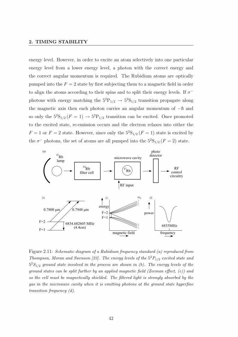
2. TIMING STABILITY
energy level. However, in order to excite an atom selectively into one particular
energy level from a lower energy level, a photon with the correct energy and
the correct angular momentum is required. The Rubidium atoms are optically
pumped into the F = 2 state by first subjecting them to a magnetic field in order
to align the atoms according to their spins and to split their energy levels. If σ−
photons with energy matching the 52P1/2 → 52S1/2 transition propagate along
the magnetic axis then each photon carries an angular momentum of −~ and
so only the 52S1/2 (F = 1) → 52P1/2 transition can be excited. Once promoted
to the excited state, re-emission occurs and the electron relaxes into either the
F = 1 or F = 2 state. However, since only the 52S1/2 (F = 1) state is excited by
the σ− photons, the set of atoms are all pumped into the 52S1/2 (F = 2) state.
Figure 2.11: Schematic diagram of a Rubidium frequency standard (a) reproduced fromThompson, Moran and Swenson [23]. The energy levels of the 52P1/2 excited state and52S1/2 ground state involved in the process are shown in (b). The energy levels of theground states can be split further by an applied magnetic field (Zeeman effect, (c)) andso the cell must be magnetically shielded. The filtered light is strongly absorbed by thegas in the microwave cavity when it is emitting photons at the ground state hyperfinetransition frequency (d).
42
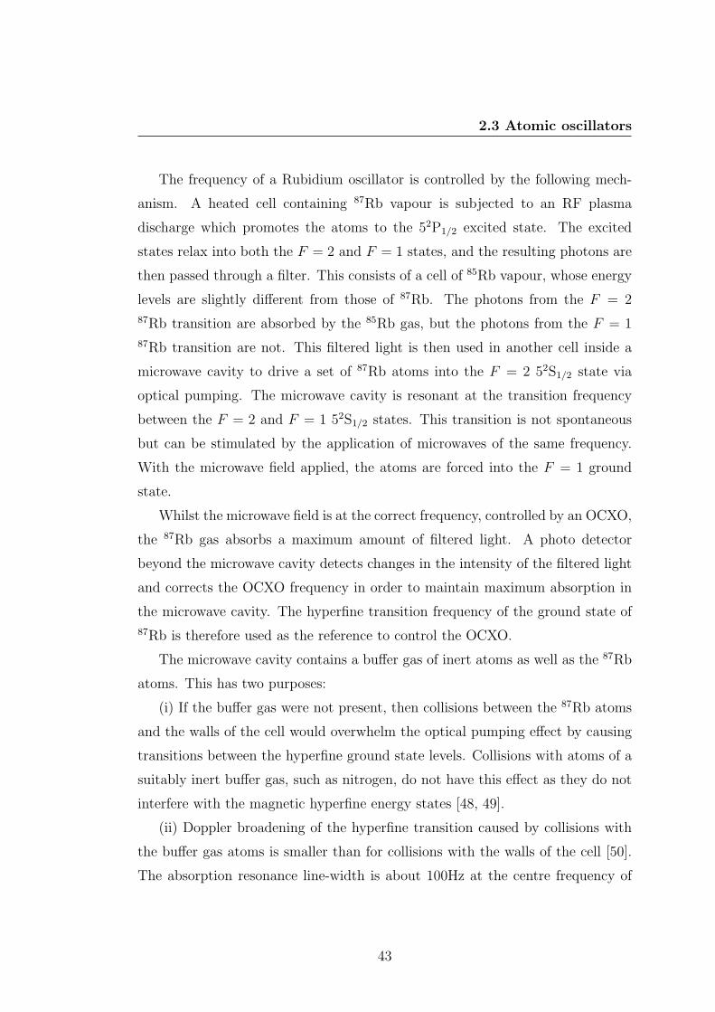
2.3 Atomic oscillators
The frequency of a Rubidium oscillator is controlled by the following mech-
anism. A heated cell containing 87Rb vapour is subjected to an RF plasma
discharge which promotes the atoms to the 52P1/2 excited state. The excited
states relax into both the F = 2 and F = 1 states, and the resulting photons are
then passed through a filter. This consists of a cell of 85Rb vapour, whose energy
levels are slightly different from those of 87Rb. The photons from the F = 2
87Rb transition are absorbed by the 85Rb gas, but the photons from the F = 1
87Rb transition are not. This filtered light is then used in another cell inside a
microwave cavity to drive a set of 87Rb atoms into the F = 2 52S1/2 state via
optical pumping. The microwave cavity is resonant at the transition frequency
between the F = 2 and F = 1 52S1/2 states. This transition is not spontaneous
but can be stimulated by the application of microwaves of the same frequency.
With the microwave field applied, the atoms are forced into the F = 1 ground
state.
Whilst the microwave field is at the correct frequency, controlled by an OCXO,
the 87Rb gas absorbs a maximum amount of filtered light. A photo detector
beyond the microwave cavity detects changes in the intensity of the filtered light
and corrects the OCXO frequency in order to maintain maximum absorption in
the microwave cavity. The hyperfine transition frequency of the ground state of
87Rb is therefore used as the reference to control the OCXO.
The microwave cavity contains a buffer gas of inert atoms as well as the 87Rb
atoms. This has two purposes:
(i) If the buffer gas were not present, then collisions between the 87Rb atoms
and the walls of the cell would overwhelm the optical pumping effect by causing
transitions between the hyperfine ground state levels. Collisions with atoms of a
suitably inert buffer gas, such as nitrogen, do not have this effect as they do not
interfere with the magnetic hyperfine energy states [48, 49].
(ii) Doppler broadening of the hyperfine transition caused by collisions with
the buffer gas atoms is smaller than for collisions with the walls of the cell [50].
The absorption resonance line-width is about 100Hz at the centre frequency of
43
2. TIMING STABILITY
6,834,682,605 Hz, and corresponds to a Q of 6.834× 10⁷, a factor of nearly 1000
times greater than for a quartz crystal.
The microwave cavity is magnetically shielded to reduce the effects of stray
external magnetic fields on the Zeeman splitting [51]. A weak magnetic field
is maintained in the cavity to maintain spin alignments. The shot noise of
individually-arriving photons leads to white-frequency noise which dominates the
frequency error at short timescales.
2.3.2 Caesium beam oscillators
Caesium is an alkali metal with a single valence electron like Rubidium. A Cae-
sium beam atomic clock uses a technique similar to that used in a Rubidium
atomic clock in order to generate a reference frequency [36], but uses inhomoge-
neous magnetic fields to filter atoms of the required electronic state instead of
using optical pumping.
The ground electronic state of 133Cs is split into two levels (F = 4 and F = 3),
depending on whether the spin of the unpaired valence electron is aligned parallel
to or anti-parallel to the nuclear spin. The transition frequency between these
states is 9,192,631,770 Hz and is used as the primary reference defining the length
of the SI second [52].
Atoms of Caesium are evaporated by an oven and move in a beam along a
confining cell through a number of stages (see Figure 2.12 below). They are first
filtered by a magnet according to their energy configurations, with the higher-
energy atoms (F = 4) following a different path through the magnetic field than
the lower-energy atoms. Only the beam of F = 3 atoms is directed into the
interaction region. The higher-energy beam is discarded. An OCXO driving a
dual microwave cavity (known as a Ramsey cavity [53]) tuned to 9,192,631,770
Hz is used to excite the F = 3 atoms into the F = 4 energy state. The Ramsey
cavity consists of two short microwave interaction regions of length l, separated
by a relatively large distance L, the microwaves in each cavity having almost
44
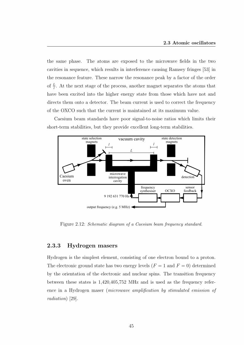
2.3 Atomic oscillators
the same phase. The atoms are exposed to the microwave fields in the two
cavities in sequence, which results in interference causing Ramsey fringes [53] in
the resonance feature. These narrow the resonance peak by a factor of the order
of Ll. At the next stage of the process, another magnet separates the atoms that
have been excited into the higher energy state from those which have not and
directs them onto a detector. The beam current is used to correct the frequency
of the OXCO such that the current is maintained at its maximum value.
Caesium beam standards have poor signal-to-noise ratios which limits their
short-term stabilities, but they provide excellent long-term stabilities.
Figure 2.12: Schematic diagram of a Caesium beam frequency standard.
2.3.3 Hydrogen masers
Hydrogen is the simplest element, consisting of one electron bound to a proton.
The electronic ground state has two energy levels (F = 1 and F = 0) determined
by the orientation of the electronic and nuclear spins. The transition frequency
between these states is 1,420,405,752 MHz and is used as the frequency refer-
ence in a Hydrogen maser (microwave amplification by stimulated emission of
radiation) [29].
45
2. TIMING STABILITY
A schematic diagram of the Hydrogen maser is given in Figure 2.13 below.
Hydrogen from a storage tank is excited by an RF discharge and passes through
a state-selecting magnet which separates the F = 1 and F = 0 states. The atoms
in the upper state are directed into a microwave cavity resonant at 1,420,405,752
MHz. The cavity is shielded from external magnetic fields, and a solenoid provides
a weak homogeneous magnetic field inside the cavity. This field slightly splits the
hyperfine levels and allows the microwave radiation injected into the cavity to
stimulate transitions from the F = 1,mF = 0 state to the F = 0,mF = 0 state
while minimising transitions from the F = 1,mF = 1 state. Transitions with
∆mF = 0 have frequencies independent of applied weak magnetic fields to a first
approximation, and so slight variations in local magnetic field do not change the
reference frequency.
The maser oscillates if (a) the cavity is tuned close to the transition frequency
and (b) the power applied to the cavity is greater than the power lost inside
it. In an active maser, the stimulated emissions of the atomic medium are self-
sustaining and the addition of microwaves at the resonant frequency from an
external source is not required. In a passive maser, this injection of energy is
required. In an active maser, a probe in the cavity measures the frequency of
the radiation emitted by the atomic transitions and the measurement is used to
phase lock an OCXO. In a passive maser, the OCXO controls the frequency of the
microwave radiation injected into the cavity to stimulate the maser process. A
feedback circuit is used to adjust the OCXO frequency to maintain the maximum
level of stimulated emission.
Active masers are inherently more stable than passive ones, but are also more
expensive because of the quality of the cavity required in order to maintain self-
sustained stimulated emission. Active Hydrogen masers provide very stable fre-
quencies over periods of 1 second to 1 day. In a 1 hour averaging time, active
Hydrogen masers exceed the stabilities of the best known Caesium beam oscil-
lators by up to a factor of 100, with typical Allan deviations of about 2× 10⁻¹⁵
[54].
46
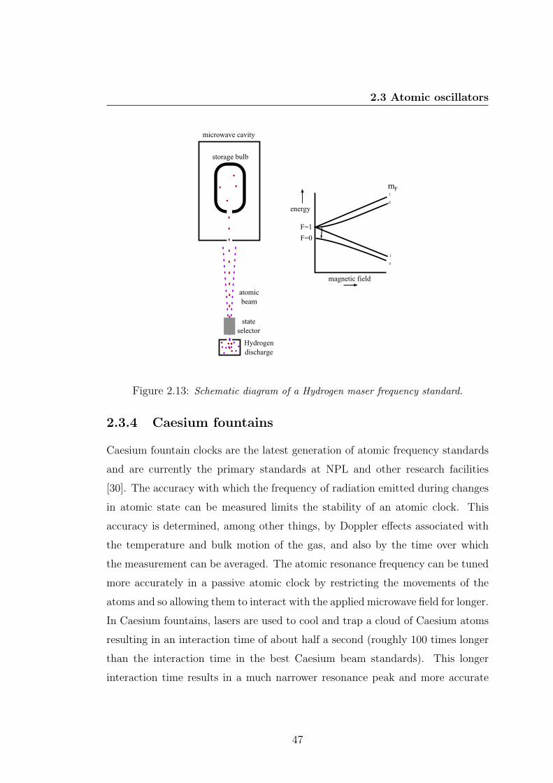
2.3 Atomic oscillators
Figure 2.13: Schematic diagram of a Hydrogen maser frequency standard.
2.3.4 Caesium fountains
Caesium fountain clocks are the latest generation of atomic frequency standards
and are currently the primary standards at NPL and other research facilities
[30]. The accuracy with which the frequency of radiation emitted during changes
in atomic state can be measured limits the stability of an atomic clock. This
accuracy is determined, among other things, by Doppler effects associated with
the temperature and bulk motion of the gas, and also by the time over which
the measurement can be averaged. The atomic resonance frequency can be tuned
more accurately in a passive atomic clock by restricting the movements of the
atoms and so allowing them to interact with the applied microwave field for longer.
In Caesium fountains, lasers are used to cool and trap a cloud of Caesium atoms
resulting in an interaction time of about half a second (roughly 100 times longer
than the interaction time in the best Caesium beam standards). This longer
interaction time results in a much narrower resonance peak and more accurate
47
2. TIMING STABILITY
OCXO tuning, hence higher frequency stability. Caesium fountain frequency
standards out-perform Hydrogen masers on timescales longer than about one
month [30].
2.3.5 Optical atomic clocks
Optical atomic clocks are expected to provide much higher frequency stabilities
than current atomic standards [33, 34]. Since the frequency of optical radia-
tion is five orders of magnitude higher than microwave frequencies, 105 optical
oscillations can in principle be counted and averaged in the same time as one
microwave oscillation. An optical standard therefore should be roughly 105 times
more stable. Optical transitions usually have narrower line-widths too, resulting
in a further improvement in stability. However, optical frequencies are difficult
to measure accurately using standard electronic techniques [35] and optical tran-
sitions are also often ‘forbidden’ transitions, so are weak.
2.4 Measurements with two Rb frequency stan-
dards
The experiments discussed in this thesis involved measuring the signal flight time
along a path from a transmitter to a receiver. Efratom Rubidium frequency
standards were used in the apparatus, and tests were performed to characterise
their performance.
It is best to measure the signal flight time along a path from a transmitter to a
receiver using the same timing reference for the apparatus at each end. However,
this would at least require very long cables, which would be impractical and which
would, in any case, introduce further problems. In practise, two references must
be used. Frequency references of the same design should, in principle, output
identical frequencies, but in reality one drifts relative to the other so that at
any time there is a phase difference φ(t) between them. This varies over time
48
2.5 Measurements of the stabilities of FRK-H Rb oscillators
according to
φ(t) = φ0 + φt+ higher order terms, (2.22)
where φ0 is the phase difference at time t = 0 (corresponding to a synchronisation
point). Two clocks attached to these free-running frequency references would not
record identical times at the same instant (for t > 0), but if the value of φ(t)
is known in full (i.e. not just modulo 2π), then the time according to one clock
can be corrected to match the time according to the other. Therefore, if the two
clocks are used to gather data in separate locations, the data streams can be
aligned such that the corrected recordings represent simultaneous measurements.
The correction process is straightforward if the higher-order terms in equation
2.22 can be ignored, i.e.
φ (t2)− φ (t1) = φ (t2 − t1) , (2.23)
where φ (t1) and φ (t2) are measurements of the phase difference of the two clocks
at the beginning and end of the recording period. These measurements can then
be used to determine the value of φ and so the full phase difference between the
clocks at any point during the experiment can be calculated.
The accuracy of this method is limited by (a) the size of the frequency differ-
ence between the oscillators and (b) the assumption that the phase drift during
the experiment is linear. The frequency difference needs to be small enough such
that the sampling windows of the two sets of apparatus overlap in time for all
of the measurements during the experiment. The linearity of the phase drift,
and hence the accuracy of the phase correction technique, is determined by the
stabilities of the oscillators.
2.5 Measurements of the stabilities of FRK-H
Rb oscillators
The cumulative phase difference between two FRK-H Rb oscillators was measured
using the apparatus shown in Figure 2.14 below. Each unit was mounted inside
49
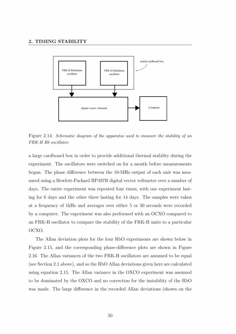
2. TIMING STABILITY
Figure 2.14: Schematic diagram of the apparatus used to measure the stability of anFRK-H Rb oscillator.
a large cardboard box in order to provide additional thermal stability during the
experiment. The oscillators were switched on for a month before measurements
began. The phase difference between the 10-MHz output of each unit was mea-
sured using a Hewlett-Packard HP497B digital vector voltmeter over a number of
days. The entire experiment was repeated four times, with one experiment last-
ing for 6 days and the other three lasting for 14 days. The samples were taken
at a frequency of 1kHz and averages over either 5 or 30 seconds were recorded
by a computer. The experiment was also performed with an OCXO compared to
an FRK-H oscillator to compare the stability of the FRK-H units to a particular
OCXO.
The Allan deviation plots for the four RbO experiments are shown below in
Figure 2.15, and the corresponding phase-difference plots are shown in Figure
2.16. The Allan variances of the two FRK-H oscillators are assumed to be equal
(see Section 2.1 above), and so the RbO Allan deviations given here are calculated
using equation 2.15. The Allan variance in the OXCO experiment was assumed
to be dominated by the OXCO and no correction for the instability of the RbO
was made. The large difference in the recorded Allan deviations (shown on the
50
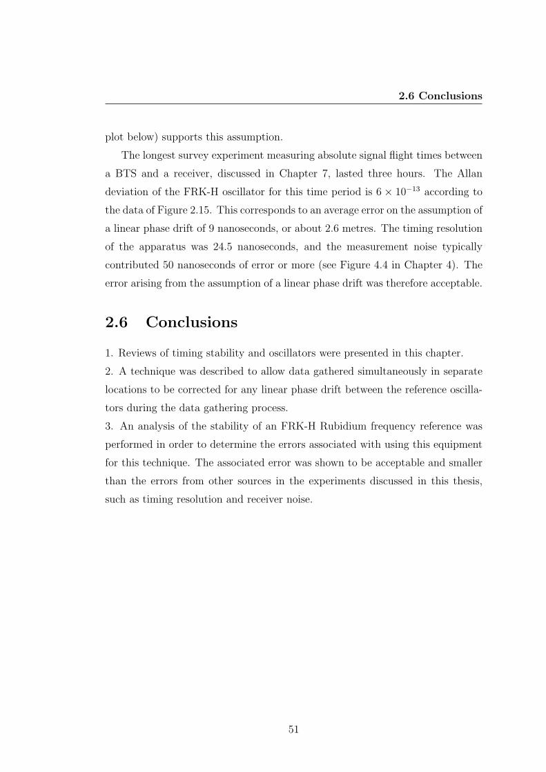
2.6 Conclusions
plot below) supports this assumption.
The longest survey experiment measuring absolute signal flight times between
a BTS and a receiver, discussed in Chapter 7, lasted three hours. The Allan
deviation of the FRK-H oscillator for this time period is 6 × 10⁻¹³ according to
the data of Figure 2.15. This corresponds to an average error on the assumption of
a linear phase drift of 9 nanoseconds, or about 2.6 metres. The timing resolution
of the apparatus was 24.5 nanoseconds, and the measurement noise typically
contributed 50 nanoseconds of error or more (see Figure 4.4 in Chapter 4). The
error arising from the assumption of a linear phase drift was therefore acceptable.
2.6 Conclusions
1. Reviews of timing stability and oscillators were presented in this chapter.
2. A technique was described to allow data gathered simultaneously in separate
locations to be corrected for any linear phase drift between the reference oscilla-
tors during the data gathering process.
3. An analysis of the stability of an FRK-H Rubidium frequency reference was
performed in order to determine the errors associated with using this equipment
for this technique. The associated error was shown to be acceptable and smaller
than the errors from other sources in the experiments discussed in this thesis,
such as timing resolution and receiver noise.
51
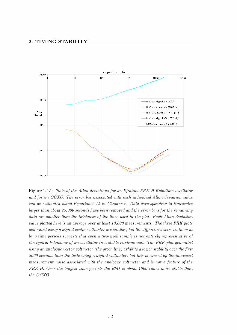
2. TIMING STABILITY
Figure 2.15: Plots of the Allan deviations for an Efratom FRK-H Rubidium oscillatorand for an OCXO. The error bar associated with each individual Allan deviation valuecan be estimated using Equation 2.14 in Chapter 2. Data corresponding to timescaleslarger than about 25,000 seconds have been removed and the error bars for the remainingdata are smaller than the thickness of the lines used in the plot. Each Allan deviationvalue plotted here is an average over at least 10,000 measurements. The three FRK plotsgenerated using a digital vector voltmeter are similar, but the differences between them atlong time periods suggests that even a two-week sample is not entirely representative ofthe typical behaviour of an oscillator in a stable environment. The FRK plot generatedusing an analogue vector voltmeter (the green line) exhibits a lower stability over the first2000 seconds than the tests using a digital voltmeter, but this is caused by the increasedmeasurement noise associated with the analogue voltmeter and is not a feature of theFRK-H. Over the longest time periods the RbO is about 1000 times more stable thanthe OCXO.
52
2.6 Conclusions
0 2 4 6 8 10 12 14
x 105
−15
−10
−5
0
5
10
15
20
25
30
time (seconds)
phasedifference
(wavelengths)
2005 test2007 test (i)2007 test (ii)2007 test (ii)
Figure 2.16: The phase differences between the 10MHz outputs of two Rubidium os-cillators in four experiments. The variation in the plots demonstrates that even a twoweek data sample is still not entirely representative of the typical behaviour of an RbO
53

2. TIMING STABILITY
54
Chapter 3
Time of flight measurements on
cellular networks
3.1 Methods
Two methods can be used to measure the signal flight times between a GSM
transmitter and a receiver. They can be described as the interferometric method
and the network-synchronised method.
3.1.1 Interferometric method
Two identical sets of apparatus are used in the interferometric method to gather
data simultaneously at a reference position and at a position of interest. A
synchronised pair of highly-stable clocks is required to ensure that the recordings
occur simultaneously. The difference in signal arrival times at the two locations
is determined by cross-correlating the sampled data sets. The maximum absolute
value of the cross-correlation function (referred to as ‘the peak’) is at the centre, or
zero-offset point, of the cross-correlation function for two locations with identical
signal flight times. For a peak at any other position, the difference in arrival
times may be calculated by dividing the number of samples between the peak
and the centre of the cross-correlation function by the sampling frequency. The
55
3. TIME OF FLIGHT MEASUREMENTS ON CELLULARNETWORKS
time of flight (TOF) of a signal from the BTS to the position of interest can be
estimated directly from this offset if one set of apparatus is at the BTS itself.
Different methods of estimating the TOF from measurements of the cross-
correlation function are discussed in Chapter 6. In the experiments presented
in this thesis, the maximum absolute value of the cross-correlation function was
used as the estimator.
An advantage of the interferometric technique is that it filters out all common-
mode variations, such as oscillations and drifts in the signal caused by the base
station’s electronics or its frequency standard. Any variations caused by the
propagation path and multipath interference can therefore be studied directly. A
disadvantage of this technique is that it requires two sets of expensive apparatus
and two operators.
3.1.2 Network-synchronised method
The network-synchronised method relies on the transmission of a known code
word at regular intervals from each BTS. On GSM networks, the code word
is called the Extended Training Sequence (ETS) and it is transmitted during a
synchronisation burst (SCB) on the logical broadcast control channel (BCCH).
The measuring equipment is programmed to record data at a multiple of the
same regular interval so that the ETS appears at the same position in the data
stream every time for a stationary receiver. This position can be found by cross-
correlating the data stream with a copy of the ETS. The maximum value of the
modulus of the cross-correlation function marks the position of the ETS in the
signal, and is referred to here as the SCB peak.
For a stationary receiver, variations in the position of the SCB peak are caused
by (a) instabilities of the frequency references in the BTS or the measuring ap-
paratus, (b) transmitter based errors such as maintenance work at the BTS, (c)
changes in the propagation path, and (d) signal interference effects at the receiver.
As the receiving equipment is moved relative to the base station, the signal TOF
56
3.1 Methods
changes and the position of the SCB peak in the data recordings varies accord-
ingly. The SCB peak position corresponding to zero distance from the BTS can
be calibrated by making a recording at the base station itself during the exper-
iment. The number of samples between this calibration SCB peak and an SCB
peak recorded in a position of interest, divided by the sampling frequency, gives
an estimate of the TOF of the signal from the base station to the position of
interest.
The SCB peak position is only expected to be stationary with time for a
stationary receiver if the frequency references in the BTS and the measuring
apparatus both remain exactly on their nominal frequencies, or drift in exactly
the same fashion such that their difference remains the same. In practise neither
of these are situations are likely, but the systematic error caused by a relative drift
between the oscillators can be corrected. A constant offset in the frequencies of the
two references results in the SCB peak position drifting at a constant rate. Such
a linear drift can be corrected easily by performing calibration measurements at
the BTS at the beginning and end of an experiment. These measurements define
a linear slope across the recordings which can then be removed from the data set
(see Section 2.4 in Chapter 2 above).
An advantage of this method over the interferometric approach is that only
one set of apparatus and one operator are needed. A disadvantage is that this
technique does not filter out any slight variations, oscillations, non-linear drifts,
or other unwanted behaviour affecting the base station’s transmission times, but
instead relies on the BTS frequency reference being highly stable. A set of exper-
iments was performed to test the viability of the network-synchronised approach
(see Chapter 4 below). For base stations with highly-stable and consistent sig-
nals, the network-synchronised method can be as accurate as the interferometric
approach but without the need for as much equipment and manpower.
The signal stabilities of BTSs with highly-stable frequency references are dom-
inated by the level of measurement noise in the system over periods of a few hours
57
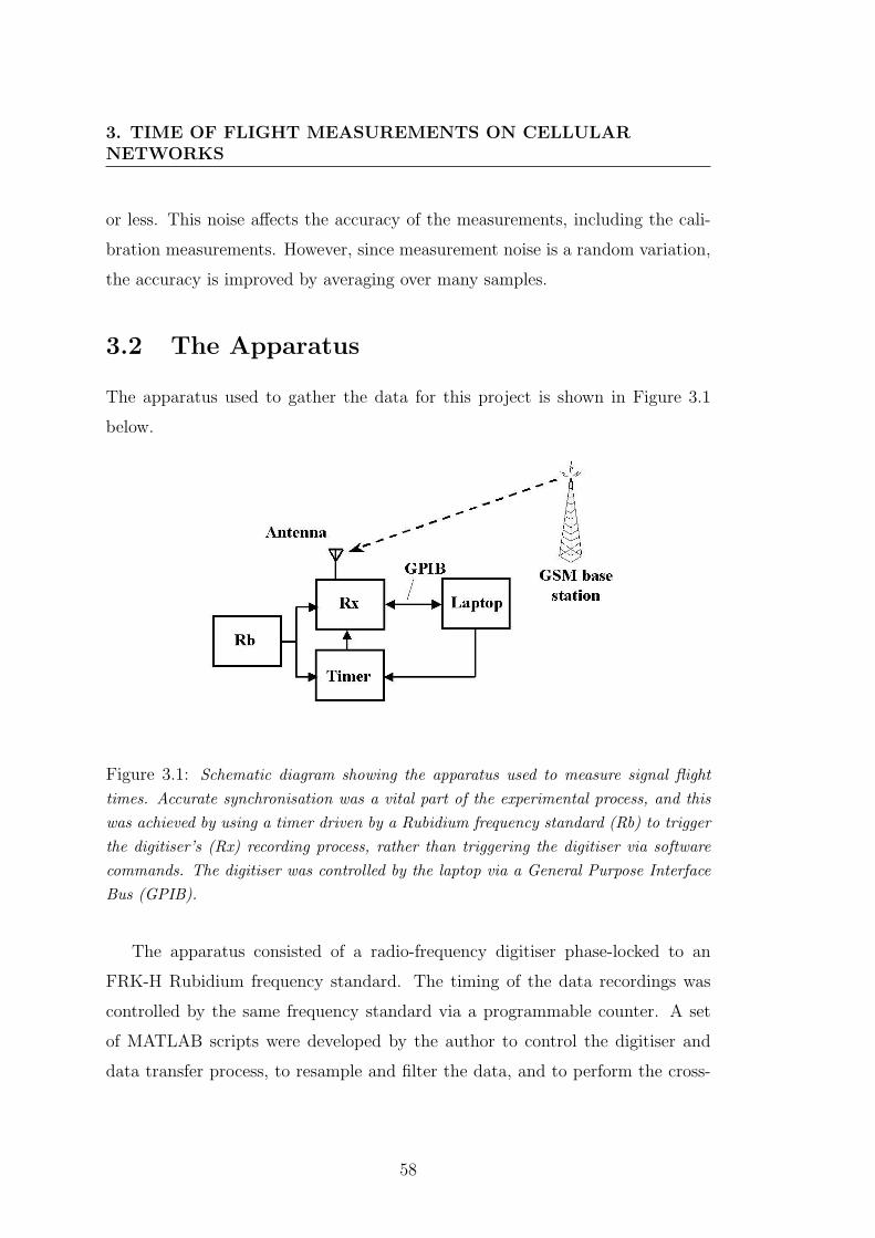
3. TIME OF FLIGHT MEASUREMENTS ON CELLULARNETWORKS
or less. This noise affects the accuracy of the measurements, including the cali-
bration measurements. However, since measurement noise is a random variation,
the accuracy is improved by averaging over many samples.
3.2 The Apparatus
The apparatus used to gather the data for this project is shown in Figure 3.1
below.
Figure 3.1: Schematic diagram showing the apparatus used to measure signal flighttimes. Accurate synchronisation was a vital part of the experimental process, and thiswas achieved by using a timer driven by a Rubidium frequency standard (Rb) to triggerthe digitiser’s (Rx) recording process, rather than triggering the digitiser via softwarecommands. The digitiser was controlled by the laptop via a General Purpose InterfaceBus (GPIB).
The apparatus consisted of a radio-frequency digitiser phase-locked to an
FRK-H Rubidium frequency standard. The timing of the data recordings was
controlled by the same frequency standard via a programmable counter. A set
of MATLAB scripts were developed by the author to control the digitiser and
data transfer process, to resample and filter the data, and to perform the cross-
58
3.2 The Apparatus
correlation processes. The digitiser’s recording process was not triggered by soft-
ware commands, but was controlled directly by the output from the Rubidium
atomic frequency reference via the timer. At the end of each timing period, the
timer output a pulse which triggered the digitiser’s capture sequence.
Each part of the apparatus and each stage of the MATLAB processing are de-
scribed in more detail below. One set of apparatus was required for the network-
synchronised approach, and two sets were required for the interferometric ap-
proach.
3.2.1 Radio frequency digitiser
The digitiser used was an IFR 2319E model [55], capable of recording a maximum
of one million complex samples at rates of 2.04 MHz, 4.08 MHz, 8.16 MHz or 16.32
MHz, over a frequency range of 500 MHz to 2 GHz, and with a bandwidth of up
to 10 MHz. The maximum length of an individual recording was therefore 0.49
seconds (one million samples at 2.04 MHz). The bandwidth of a GSM signal is
140kHz, and so any of these sampling frequencies satisfied the Nyquist-Shannon
sampling criterion [56]. The lowest sampling frequency was chosen in order to
maximise the amount of data that could be recorded in one measurement. The
original signal could therefore be fully reconstructed from the sampled data before
a time-of-flight calculation was performed. Timing resolution was improved using
interpolation, and averaging the values from a number of recordings at a given
position reduced the error caused by system noise. The digitizer output data in
the form of I and Q complex samples, such that the magnitude and phase of a
given sample were stored in cartesian coordinates rather than polar coordinates.
3.2.2 Triggering and synchronisation
The most important factor in gathering useful data was timing the recordings with
the highest accuracy possible. An FRK-H Rubidium Frequency Standard (RFS)
controlled the timing of the data captures via the counter and also provided the
59
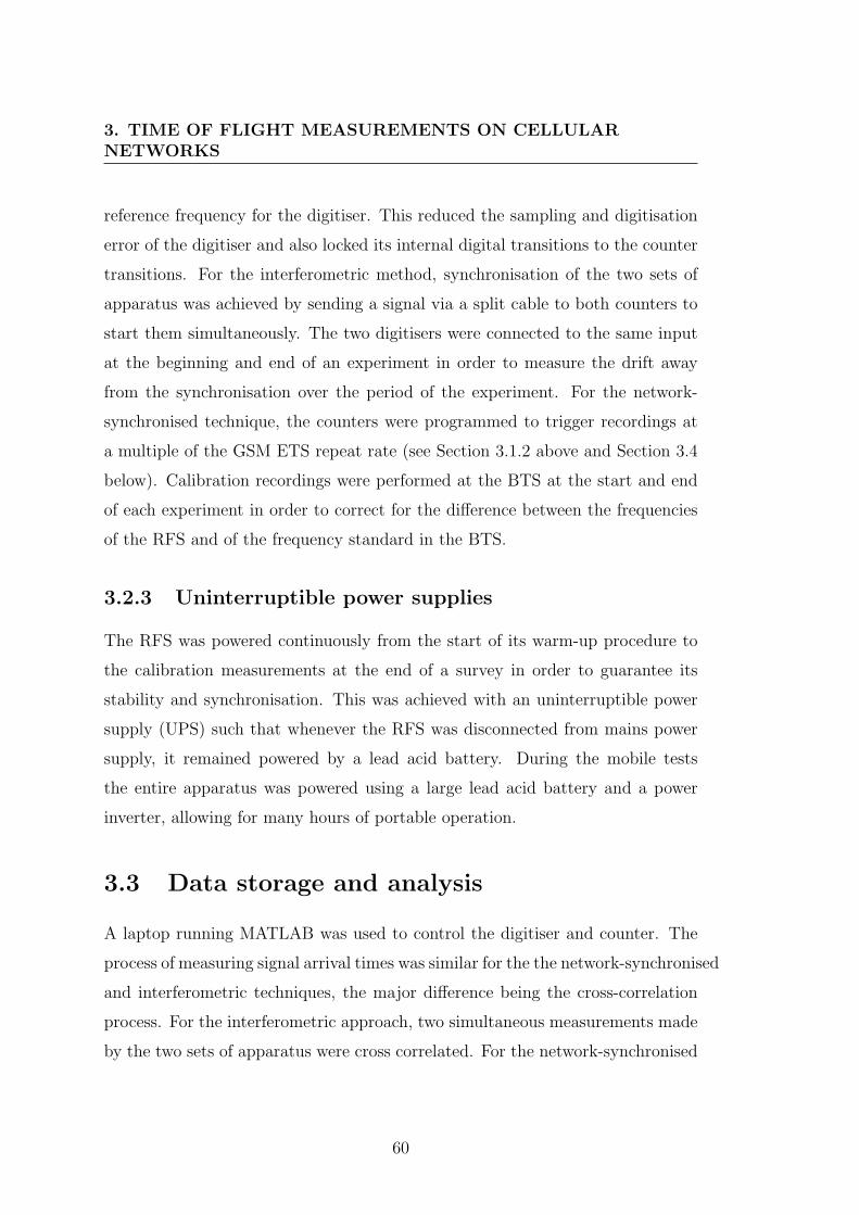
3. TIME OF FLIGHT MEASUREMENTS ON CELLULARNETWORKS
reference frequency for the digitiser. This reduced the sampling and digitisation
error of the digitiser and also locked its internal digital transitions to the counter
transitions. For the interferometric method, synchronisation of the two sets of
apparatus was achieved by sending a signal via a split cable to both counters to
start them simultaneously. The two digitisers were connected to the same input
at the beginning and end of an experiment in order to measure the drift away
from the synchronisation over the period of the experiment. For the network-
synchronised technique, the counters were programmed to trigger recordings at
a multiple of the GSM ETS repeat rate (see Section 3.1.2 above and Section 3.4
below). Calibration recordings were performed at the BTS at the start and end
of each experiment in order to correct for the difference between the frequencies
of the RFS and of the frequency standard in the BTS.
3.2.3 Uninterruptible power supplies
The RFS was powered continuously from the start of its warm-up procedure to
the calibration measurements at the end of a survey in order to guarantee its
stability and synchronisation. This was achieved with an uninterruptible power
supply (UPS) such that whenever the RFS was disconnected from mains power
supply, it remained powered by a lead acid battery. During the mobile tests
the entire apparatus was powered using a large lead acid battery and a power
inverter, allowing for many hours of portable operation.
3.3 Data storage and analysis
A laptop running MATLAB was used to control the digitiser and counter. The
process of measuring signal arrival times was similar for the the network-synchronised
and interferometric techniques, the major difference being the cross-correlation
process. For the interferometric approach, two simultaneous measurements made
by the two sets of apparatus were cross correlated. For the network-synchronised
60
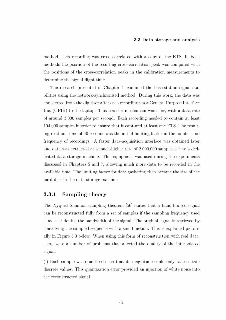
3.3 Data storage and analysis
method, each recording was cross correlated with a copy of the ETS. In both
methods the position of the resulting cross-correlation peak was compared with
the positions of the cross-correlation peaks in the calibration measurements to
determine the signal flight time.
The research presented in Chapter 4 examined the base-station signal sta-
bilities using the network-synchronised method. During this work, the data was
transferred from the digitiser after each recording via a General Purpose Interface
Bus (GPIB) to the laptop. This transfer mechanism was slow, with a data rate
of around 3,000 samples per second. Each recording needed to contain at least
104,000 samples in order to ensure that it captured at least one ETS. The result-
ing read-out time of 40 seconds was the initial limiting factor in the number and
frequency of recordings. A faster data-acquisition interface was obtained later
and data was extracted at a much-higher rate of 2,000,000 samples s−1 to a ded-
icated data storage machine. This equipment was used during the experiments
discussed in Chapters 5 and 7, allowing much more data to be recorded in the
available time. The limiting factor for data gathering then became the size of the
hard disk in the data-storage machine.
3.3.1 Sampling theory
The Nyquist-Shannon sampling theorem [56] states that a band-limited signal
can be reconstructed fully from a set of samples if the sampling frequency used
is at least double the bandwidth of the signal. The original signal is retrieved by
convolving the sampled sequence with a sinc function. This is explained pictori-
ally in Figure 3.3 below. When using this form of reconstruction with real data,
there were a number of problems that affected the quality of the interpolated
signal.
(i) Each sample was quantised such that its magnitude could only take certain
discrete values. This quantisation error provided an injection of white noise into
the reconstructed signal.
61
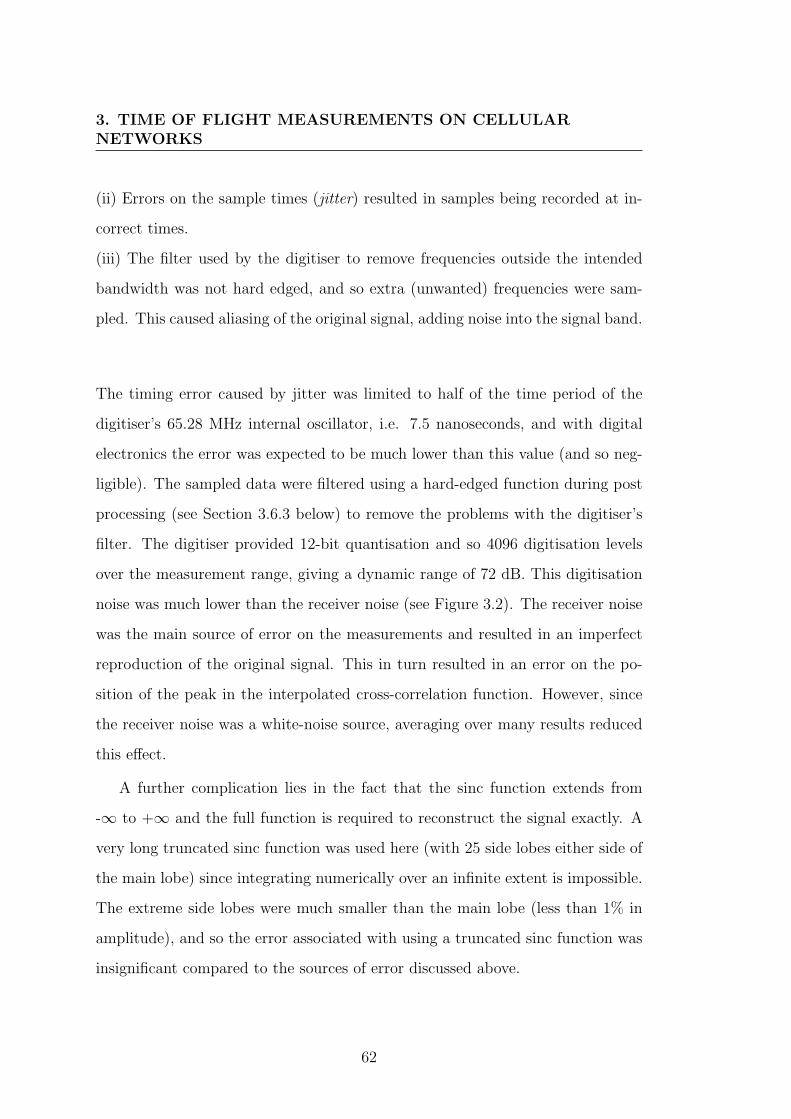
3. TIME OF FLIGHT MEASUREMENTS ON CELLULARNETWORKS
(ii) Errors on the sample times (jitter) resulted in samples being recorded at in-
correct times.
(iii) The filter used by the digitiser to remove frequencies outside the intended
bandwidth was not hard edged, and so extra (unwanted) frequencies were sam-
pled. This caused aliasing of the original signal, adding noise into the signal band.
The timing error caused by jitter was limited to half of the time period of the
digitiser’s 65.28 MHz internal oscillator, i.e. 7.5 nanoseconds, and with digital
electronics the error was expected to be much lower than this value (and so neg-
ligible). The sampled data were filtered using a hard-edged function during post
processing (see Section 3.6.3 below) to remove the problems with the digitiser’s
filter. The digitiser provided 12-bit quantisation and so 4096 digitisation levels
over the measurement range, giving a dynamic range of 72 dB. This digitisation
noise was much lower than the receiver noise (see Figure 3.2). The receiver noise
was the main source of error on the measurements and resulted in an imperfect
reproduction of the original signal. This in turn resulted in an error on the po-
sition of the peak in the interpolated cross-correlation function. However, since
the receiver noise was a white-noise source, averaging over many results reduced
this effect.
A further complication lies in the fact that the sinc function extends from
-∞ to +∞ and the full function is required to reconstruct the signal exactly. A
very long truncated sinc function was used here (with 25 side lobes either side of
the main lobe) since integrating numerically over an infinite extent is impossible.
The extreme side lobes were much smaller than the main lobe (less than 1% in
amplitude), and so the error associated with using a truncated sinc function was
insignificant compared to the sources of error discussed above.
62
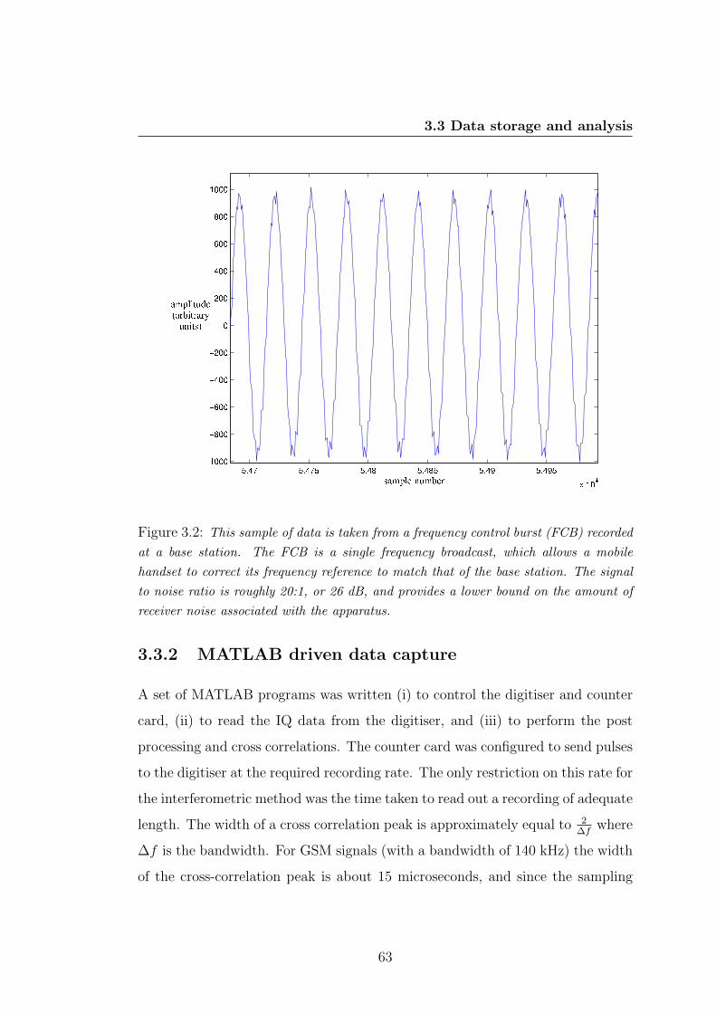
3.3 Data storage and analysis
Figure 3.2: This sample of data is taken from a frequency control burst (FCB) recordedat a base station. The FCB is a single frequency broadcast, which allows a mobilehandset to correct its frequency reference to match that of the base station. The signalto noise ratio is roughly 20:1, or 26 dB, and provides a lower bound on the amount ofreceiver noise associated with the apparatus.
3.3.2 MATLAB driven data capture
A set of MATLAB programs was written (i) to control the digitiser and counter
card, (ii) to read the IQ data from the digitiser, and (iii) to perform the post
processing and cross correlations. The counter card was configured to send pulses
to the digitiser at the required recording rate. The only restriction on this rate for
the interferometric method was the time taken to read out a recording of adequate
length. The width of a cross correlation peak is approximately equal to 2∆f
where
∆f is the bandwidth. For GSM signals (with a bandwidth of 140 kHz) the width
of the cross-correlation peak is about 15 microseconds, and since the sampling
63
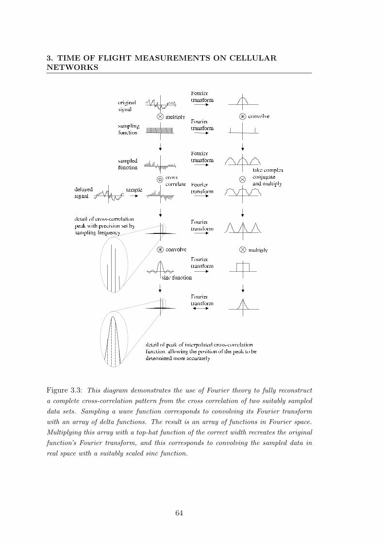
3. TIME OF FLIGHT MEASUREMENTS ON CELLULARNETWORKS
Figure 3.3: This diagram demonstrates the use of Fourier theory to fully reconstructa complete cross-correlation pattern from the cross correlation of two suitably sampleddata sets. Sampling a wave function corresponds to convolving its Fourier transformwith an array of delta functions. The result is an array of functions in Fourier space.Multiplying this array with a top-hat function of the correct width recreates the originalfunction’s Fourier transform, and this corresponds to convolving the sampled data inreal space with a suitably scaled sinc function.
64
3.3 Data storage and analysis
rate used was 2.04 MHz, a minimum of 30 samples were needed to capture a full
cross-correlation peak. Further samples were then needed to allow for any drift
between the oscillators in the apparatus, and to measure the displacement of the
peak caused by path length differences between the two recordings. Each sample
corresponded to a distance of about 150 metres and the oscillator drift only
accounted for a few tens of samples over the course of a few hours, so recordings
of 1000 samples were more than adequate in the interferometric technique and
were transferred by GPIB in less than a second.
The network-synchronised approach required the recordings to capture at least
one synchronisation burst without any prior knowledge of their positions in the
data stream. In order to guarantee this the minimum number of samples per
recording was 104,000 as the maximum separation between SCBs is 51 millisec-
onds (see Section 3.4 below). The GPIB readout time for recordings of this length
was 40 seconds. The fast data acquisition interface could extract a full buffer of
one million complex samples containing 10 or 11 SCBs in half a second. The trig-
gering period used for the network synchronised method needed to be a multiple
of the multiframe repeat period of 3.0613
seconds (see Section 3.4 below).
The digitiser captured a preprogrammed number of samples each time it re-
ceived a pulse from the counter, and then attempted to transmit the samples to
the data-capture machine. The digitiser remained in transfer mode only for a
certain length of time before clearing its memory ready for the next recording.
The data transfer process on both the GPIB and fast data interfaces involved
handshaking, meaning the digitiser did not transmit any data packets until it
received a signal from the data receiving device confirming that the latter was
ready. This prevented any corruption of the data, or missing samples in a data-
set. The times of each recording were stored on the laptop via a readout from
the counter.
65
3. TIME OF FLIGHT MEASUREMENTS ON CELLULARNETWORKS
3.3.3 Cross correlation
The analogue cross-correlation operation between two continuous functions f and
g is defined as
f ? g =
∫ ∞
−∞f ∗(τ)g(t+ τ) dτ. (3.1)
This cross correlation can also be evaluated by performing a series of Fourier
transforms. The Fourier transform of f and the complex conjugate of the Fourier
transform of g are first determined. The cross correlation is then given by the
inverse Fourier transform of the complex product of these two functions, as shown
below in equation 3.2.
f ? g = F[F ∗(ν)G(ν)] (3.2)
3.3.3.1 The ambiguity function
The interferometric and network-synchronised methods described above both
make use of a matched filter to detect the arrival of a signal at the receiver.
If the receiver or transmitter are moving then the received signal will be Doppler
shifted accordingly. This can in turn have a detrimental effect on the cross-
correlation function and the ability to determine the signal arrival time correctly.
The receiver and transmitters remained stationary during all measurements in
this project, but the sources of any multipath interference, such as vehicles, tree
branches, people, etc could have been moving, resulting in a Doppler-shifted-
multipath signal. The ambiguity function is a two-dimensional function of time
delay and Doppler frequency and is given by
χ(τ, f) =
∫ ∞
−∞s(t)s∗(t− τ)e−i2πftdt. (3.3)
where τ is the time delay, f is the Doppler-frequency shift and s is the complex
function under test. The ambiguity function reveals how the cross-correlation
profile of a matched filter varies as the received signal is Doppler shifted. Figure
3.4 below is a plot of the ambiguity funtion for the GSM ETS. The strong central
66
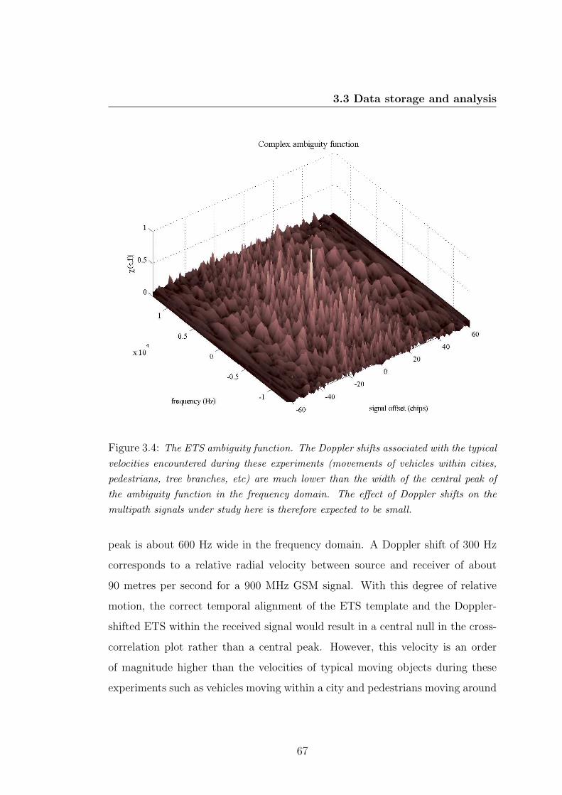
3.3 Data storage and analysis
Figure 3.4: The ETS ambiguity function. The Doppler shifts associated with the typicalvelocities encountered during these experiments (movements of vehicles within cities,pedestrians, tree branches, etc) are much lower than the width of the central peak ofthe ambiguity function in the frequency domain. The effect of Doppler shifts on themultipath signals under study here is therefore expected to be small.
peak is about 600 Hz wide in the frequency domain. A Doppler shift of 300 Hz
corresponds to a relative radial velocity between source and receiver of about
90 metres per second for a 900 MHz GSM signal. With this degree of relative
motion, the correct temporal alignment of the ETS template and the Doppler-
shifted ETS within the received signal would result in a central null in the cross-
correlation plot rather than a central peak. However, this velocity is an order
of magnitude higher than the velocities of typical moving objects during these
experiments such as vehicles moving within a city and pedestrians moving around
67
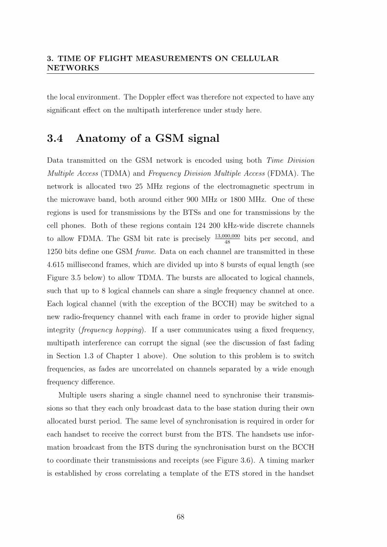
3. TIME OF FLIGHT MEASUREMENTS ON CELLULARNETWORKS
the local environment. The Doppler effect was therefore not expected to have any
significant effect on the multipath interference under study here.
3.4 Anatomy of a GSM signal
Data transmitted on the GSM network is encoded using both Time Division
Multiple Access (TDMA) and Frequency Division Multiple Access (FDMA). The
network is allocated two 25 MHz regions of the electromagnetic spectrum in
the microwave band, both around either 900 MHz or 1800 MHz. One of these
regions is used for transmissions by the BTSs and one for transmissions by the
cell phones. Both of these regions contain 124 200 kHz-wide discrete channels
to allow FDMA. The GSM bit rate is precisely 13,000,00048
bits per second, and
1250 bits define one GSM frame. Data on each channel are transmitted in these
4.615 millisecond frames, which are divided up into 8 bursts of equal length (see
Figure 3.5 below) to allow TDMA. The bursts are allocated to logical channels,
such that up to 8 logical channels can share a single frequency channel at once.
Each logical channel (with the exception of the BCCH) may be switched to a
new radio-frequency channel with each frame in order to provide higher signal
integrity (frequency hopping). If a user communicates using a fixed frequency,
multipath interference can corrupt the signal (see the discussion of fast fading
in Section 1.3 of Chapter 1 above). One solution to this problem is to switch
frequencies, as fades are uncorrelated on channels separated by a wide enough
frequency difference.
Multiple users sharing a single channel need to synchronise their transmis-
sions so that they each only broadcast data to the base station during their own
allocated burst period. The same level of synchronisation is required in order for
each handset to receive the correct burst from the BTS. The handsets use infor-
mation broadcast from the BTS during the synchronisation burst on the BCCH
to coordinate their transmissions and receipts (see Figure 3.6). A timing marker
is established by cross correlating a template of the ETS stored in the handset
68
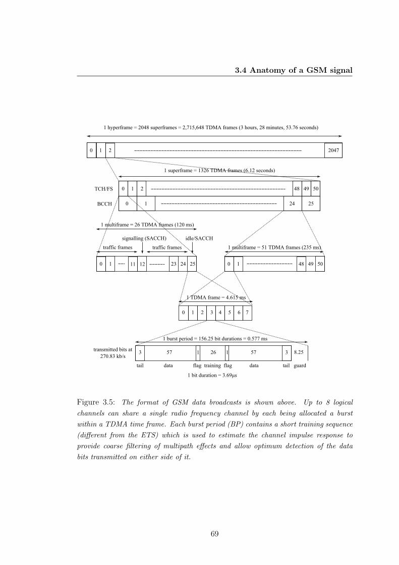
3.4 Anatomy of a GSM signal
Figure 3.5: The format of GSM data broadcasts is shown above. Up to 8 logicalchannels can share a single radio frequency channel by each being allocated a burstwithin a TDMA time frame. Each burst period (BP) contains a short training sequence(different from the ETS) which is used to estimate the channel impulse response toprovide coarse filtering of multipath effects and allow optimum detection of the databits transmitted on either side of it.
69
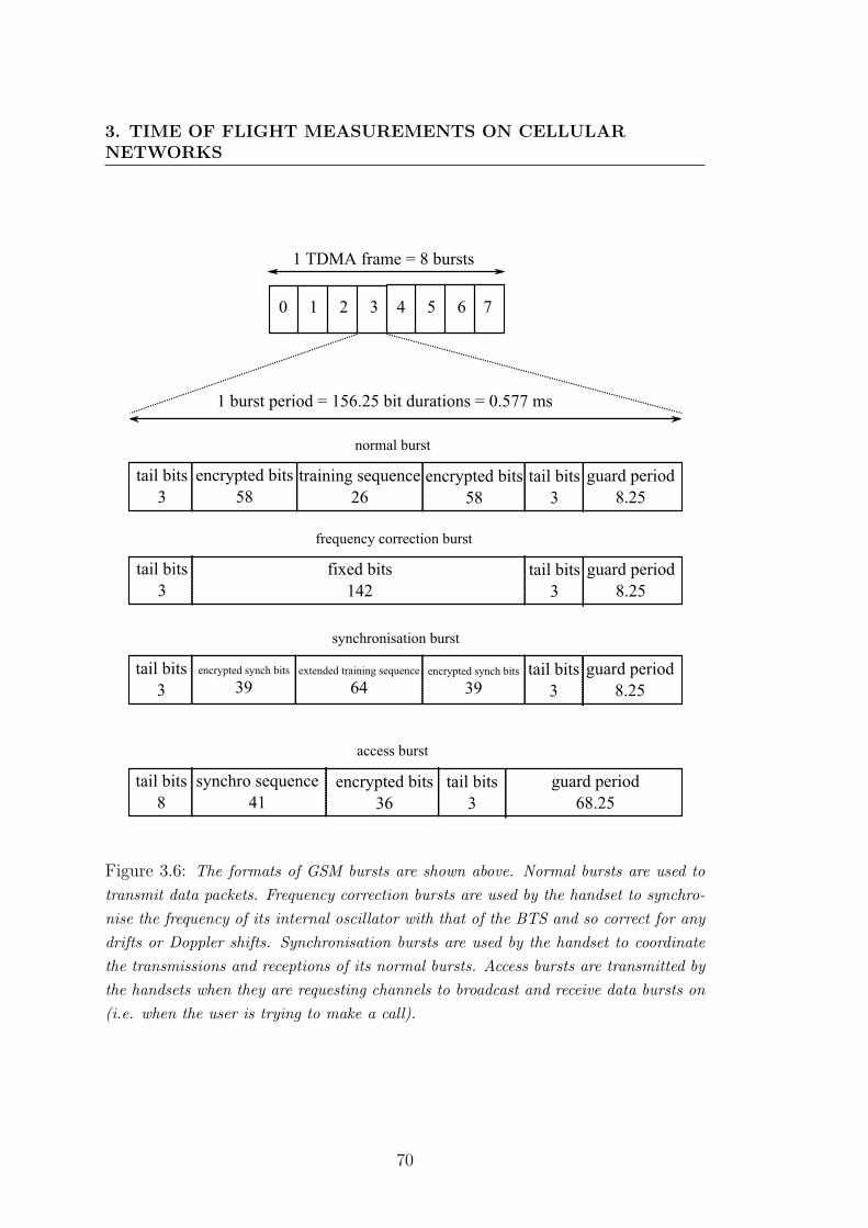
3. TIME OF FLIGHT MEASUREMENTS ON CELLULARNETWORKS
Figure 3.6: The formats of GSM bursts are shown above. Normal bursts are used totransmit data packets. Frequency correction bursts are used by the handset to synchro-nise the frequency of its internal oscillator with that of the BTS and so correct for anydrifts or Doppler shifts. Synchronisation bursts are used by the handset to coordinatethe transmissions and receptions of its normal bursts. Access bursts are transmitted bythe handsets when they are requesting channels to broadcast and receive data bursts on(i.e. when the user is trying to make a call).
70
3.4 Anatomy of a GSM signal
with the data in the SCB, allowing the time that the ETS was received in the
data stream from the BTS to be determined with a precision of roughly ±12bit.
This is used as a reference point to calculate when the phone should transmit or
expect to receive its data packets1.
The synchronisation bursts occur in a semi-regular sequence on the BCCH.
An SCB is broadcast once every ten frames (46.15 milliseconds), four times in
succession, and then broadcast again after eleven frames (50.765 milliseconds).
The sequence then repeats. This irregular sequence defines a fifty-one-frame-long
multiframe, which contains five SCBs.
Each communication burst is 148 bits long, consisting of 114 data bits, 2 flag
bits, 26 equaliser training bits (a short training sequence), and 6 tail bits. A
further 8.25 bit periods of guard time are allowed between the bursts. The 26
training bits allow an adaptive equaliser to estimate the channel impulse response
to provide coarse filtering of multipath effects and allow optimum detection of
the 57 data bits and 2 flag bits either side of it to be performed.
3.4.1 GSM digital encoding
The communication data on the GSM network are encoded digitally using Viterbi
encoding and then are modulated for transmission using Gaussian Minimum Shift
Keying (GMSK). Viterbi encoding is a type of convolution coding which provides
error-correction capabilities. The original data sequence is used to generate a
much longer sequence for transmission, but one which is created in such a way
that any parts that are missing or corrupted due to noise in the system can be
redetermined (probabilistically) using the surrounding parts of the sequence (see
Figures 3.8 to 3.11 in the post-processing section below).
1See the discussion of timing advance in Section 1.2.1 of Chapter 1
71
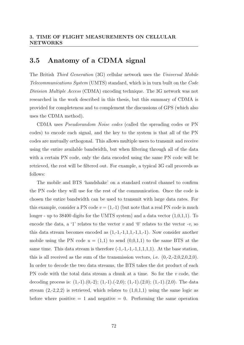
3. TIME OF FLIGHT MEASUREMENTS ON CELLULARNETWORKS
3.5 Anatomy of a CDMA signal
The British Third Generation (3G) cellular network uses the Universal Mobile
Telecommunications System (UMTS) standard, which is in turn built on the Code
Division Multiple Access (CDMA) encoding technique. The 3G network was not
researched in the work described in this thesis, but this summary of CDMA is
provided for completeness and to complement the discussions of GPS (which also
uses the CDMA method).
CDMA uses Pseudorandom Noise codes (called the spreading codes or PN
codes) to encode each signal, and the key to the system is that all of the PN
codes are mutually orthogonal. This allows multiple users to transmit and receive
using the entire available bandwidth, but when filtering through all of the data
with a certain PN code, only the data encoded using the same PN code will be
retrieved, the rest will be filtered out. For example, a typical 3G call proceeds as
follows:
The mobile and BTS ‘handshake’ on a standard control channel to confirm
the PN code they will use for the rest of the communication. Once the code is
chosen the entire bandwidth can be used to transmit with large data rates. For
this example, consider a PN code v = (1,-1) (but note that a real PN code is much
longer - up to 38400 digits for the UMTS system) and a data vector (1,0,1,1). To
encode the data, a ‘1’ relates to the vector v and ‘0’ relates to the vector -v, so
this data stream becomes encoded as (1,-1,-1,1,1,-1,1,-1). Now consider another
mobile using the PN code u = (1,1) to send (0,0,1,1) to the same BTS at the
same time. This data stream is therefore (-1,-1,-1,-1,1,1,1,1). At the base station,
this is all received as the sum of the transmission vectors, i.e. (0,-2,-2,0,2,0,2,0).
In order to decode the two data streams, the BTS takes the dot product of each
PN code with the total data stream a chunk at a time. So for the v code, the
decoding process is: (1,-1).(0,-2); (1,-1).(-2,0); (1,-1).(2,0); (1,-1).(2,0). The data
stream (2,-2,2,2) is retrieved, which relates to (1,0,1,1) using the same logic as
before where positive = 1 and negative = 0. Performing the same operation
72
3.6 The Experiments
with the u code results in retrieving the u data stream. The statistical properties
of PN codes are very similar to those of white noise, and crucially they do not
correlate with each other or a delayed copy of themselves. This behaviour also
allows the data transmissions to be asynchronous, which reduces the complexity
of the network.
3.6 The Experiments
There were two types of experiment performed for this research, (a) static tests
and (b) mobile tests. For static tests, the equipment remained in a fixed position
and the antenna either remained stationary or moved short distances. The appa-
ratus was powered via the mains supply and could be run continuously. Mobile
tests involved loading all of the equipment onto a trolley or into a car and moving
the entire apparatus between measurement points. In this case, the equipment
was powered via a large lead-acid battery and a power inverter. The battery
held enough charge for more than a day of continuous use, but in practise mobile
experiments lasted three hours or less.
Each experiment consisted of three parts: preparation, surveying, and post
processing.
3.6.1 Preparation
The preparation for each set of experiments consisted of the following stages:
(a) The Rubidium frequency standard was allowed at least forty eight hours of
warm-up time in order to maximise its stability. It was powered via an unin-
terruptible power supply and so this requirement was easily met. The digitiser
was also powered for at least a day before any experiments to allow its internal
components to reach a stable temperature.
(b) The survey route and rough positions of measurement points were planned in
advance of the experiment. This minimised the time spent gathering data and so
73
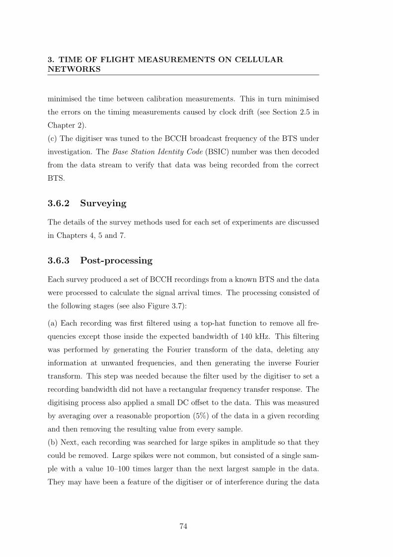
3. TIME OF FLIGHT MEASUREMENTS ON CELLULARNETWORKS
minimised the time between calibration measurements. This in turn minimised
the errors on the timing measurements caused by clock drift (see Section 2.5 in
Chapter 2).
(c) The digitiser was tuned to the BCCH broadcast frequency of the BTS under
investigation. The Base Station Identity Code (BSIC) number was then decoded
from the data stream to verify that data was being recorded from the correct
BTS.
3.6.2 Surveying
The details of the survey methods used for each set of experiments are discussed
in Chapters 4, 5 and 7.
3.6.3 Post-processing
Each survey produced a set of BCCH recordings from a known BTS and the data
were processed to calculate the signal arrival times. The processing consisted of
the following stages (see also Figure 3.7):
(a) Each recording was first filtered using a top-hat function to remove all fre-
quencies except those inside the expected bandwidth of 140 kHz. This filtering
was performed by generating the Fourier transform of the data, deleting any
information at unwanted frequencies, and then generating the inverse Fourier
transform. This step was needed because the filter used by the digitiser to set a
recording bandwidth did not have a rectangular frequency transfer response. The
digitising process also applied a small DC offset to the data. This was measured
by averaging over a reasonable proportion (5%) of the data in a given recording
and then removing the resulting value from every sample.
(b) Next, each recording was searched for large spikes in amplitude so that they
could be removed. Large spikes were not common, but consisted of a single sam-
ple with a value 10–100 times larger than the next largest sample in the data.
They may have been a feature of the digitiser or of interference during the data
74
3.6 The Experiments
Figure 3.7: Flowchart describing how the raw data was processed to generate a list ofcross-correlation peak positions.
transfer process but could not have been true samples of the GSM signal based on
the values of the surrounding samples. A large spike in the sampled data would
have resulted in a corresponding large spike in the cross-correlation profile which
could have caused an error in the peak position of the cross-correlation function.
(c) The recordings were then resampled to match the GSM bit rate, allowing all
75
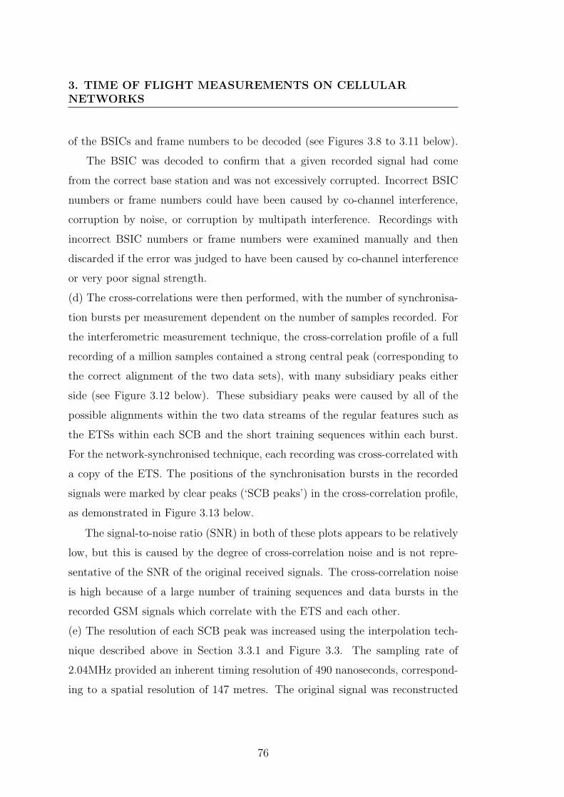
3. TIME OF FLIGHT MEASUREMENTS ON CELLULARNETWORKS
of the BSICs and frame numbers to be decoded (see Figures 3.8 to 3.11 below).
The BSIC was decoded to confirm that a given recorded signal had come
from the correct base station and was not excessively corrupted. Incorrect BSIC
numbers or frame numbers could have been caused by co-channel interference,
corruption by noise, or corruption by multipath interference. Recordings with
incorrect BSIC numbers or frame numbers were examined manually and then
discarded if the error was judged to have been caused by co-channel interference
or very poor signal strength.
(d) The cross-correlations were then performed, with the number of synchronisa-
tion bursts per measurement dependent on the number of samples recorded. For
the interferometric measurement technique, the cross-correlation profile of a full
recording of a million samples contained a strong central peak (corresponding to
the correct alignment of the two data sets), with many subsidiary peaks either
side (see Figure 3.12 below). These subsidiary peaks were caused by all of the
possible alignments within the two data streams of the regular features such as
the ETSs within each SCB and the short training sequences within each burst.
For the network-synchronised technique, each recording was cross-correlated with
a copy of the ETS. The positions of the synchronisation bursts in the recorded
signals were marked by clear peaks (‘SCB peaks’) in the cross-correlation profile,
as demonstrated in Figure 3.13 below.
The signal-to-noise ratio (SNR) in both of these plots appears to be relatively
low, but this is caused by the degree of cross-correlation noise and is not repre-
sentative of the SNR of the original received signals. The cross-correlation noise
is high because of a large number of training sequences and data bursts in the
recorded GSM signals which correlate with the ETS and each other.
(e) The resolution of each SCB peak was increased using the interpolation tech-
nique described above in Section 3.3.1 and Figure 3.3. The sampling rate of
2.04MHz provided an inherent timing resolution of 490 nanoseconds, correspond-
ing to a spatial resolution of 147 metres. The original signal was reconstructed
76
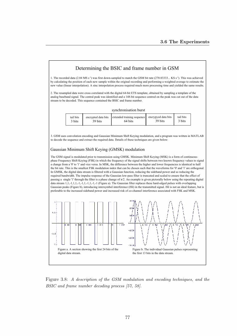
3.6 The Experiments
Figure 3.8: A description of the GSM modulation and encoding techniques, and theBSIC and frame number decoding process [57, 58].
77
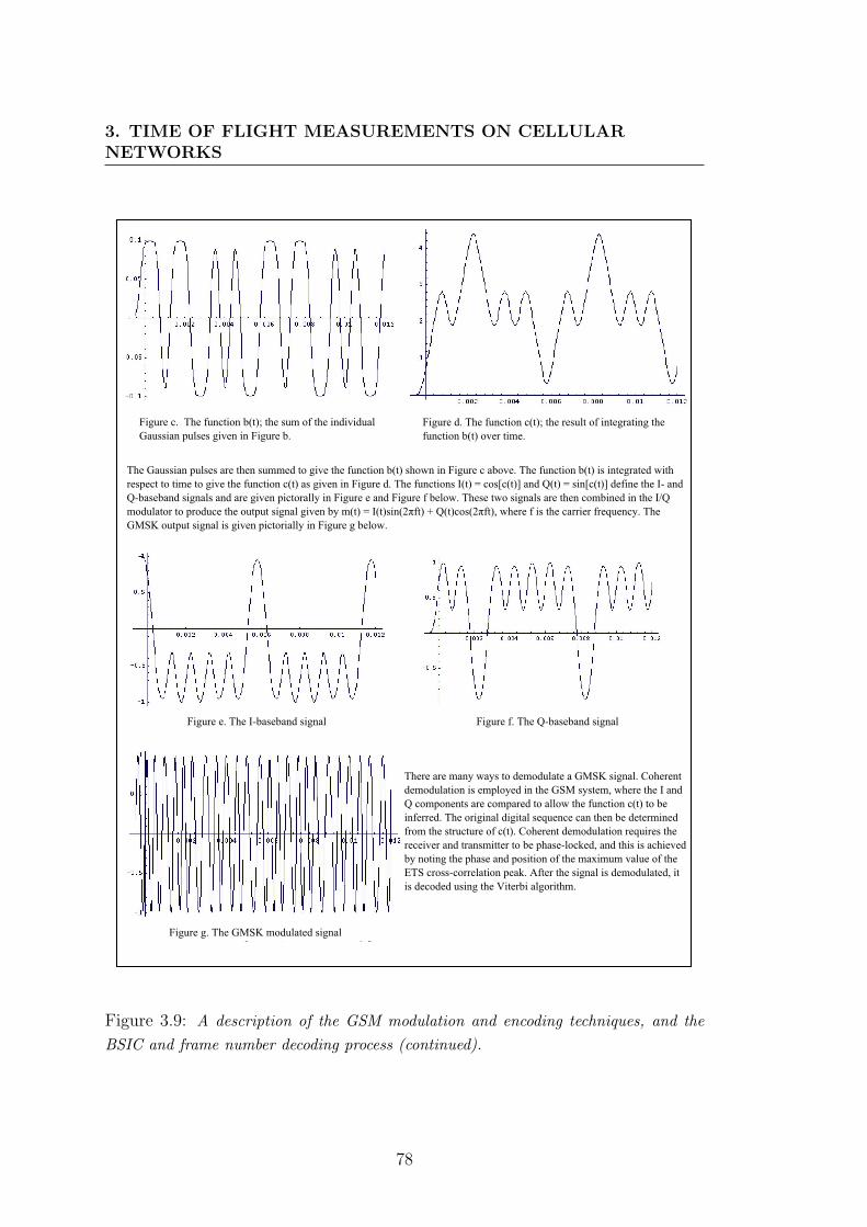
3. TIME OF FLIGHT MEASUREMENTS ON CELLULARNETWORKS
Figure 3.9: A description of the GSM modulation and encoding techniques, and theBSIC and frame number decoding process (continued).
78
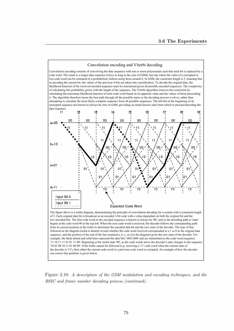
3.6 The Experiments
Figure 3.10: A description of the GSM modulation and encoding techniques, and theBSIC and frame number decoding process (continued).
79
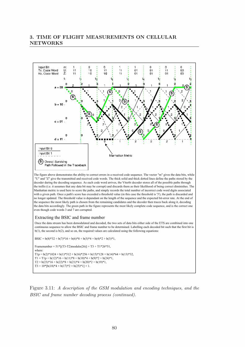
3. TIME OF FLIGHT MEASUREMENTS ON CELLULARNETWORKS
Figure 3.11: A description of the GSM modulation and encoding techniques, and theBSIC and frame number decoding process (continued).
80
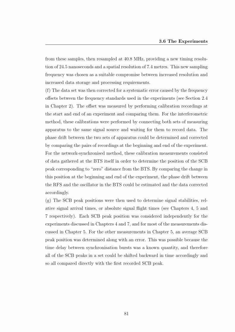
3.6 The Experiments
from these samples, then resampled at 40.8 MHz, providing a new timing resolu-
tion of 24.5 nanoseconds and a spatial resolution of 7.4 metres. This new sampling
frequency was chosen as a suitable compromise between increased resolution and
increased data storage and processing requirements.
(f) The data set was then corrected for a systematic error caused by the frequency
offsets between the frequency standards used in the experiments (see Section 2.4
in Chapter 2). The offset was measured by performing calibration recordings at
the start and end of an experiment and comparing them. For the interferometric
method, these calibrations were performed by connecting both sets of measuring
apparatus to the same signal source and waiting for them to record data. The
phase drift between the two sets of apparatus could be determined and corrected
by comparing the pairs of recordings at the beginning and end of the experiment.
For the network-synchronised method, these calibration measurements consisted
of data gathered at the BTS itself in order to determine the position of the SCB
peak corresponding to “zero” distance from the BTS. By comparing the change in
this position at the beginning and end of the experiment, the phase drift between
the RFS and the oscillator in the BTS could be estimated and the data corrected
accordingly.
(g) The SCB peak positions were then used to determine signal stabilities, rel-
ative signal arrival times, or absolute signal flight times (see Chapters 4, 5 and
7 respectively). Each SCB peak position was considered independently for the
experiments discussed in Chapters 4 and 7, and for most of the measurements dis-
cussed in Chapter 5. For the other measurements in Chapter 5, an average SCB
peak position was determined along with an error. This was possible because the
time delay between synchronisation bursts was a known quantity, and therefore
all of the SCB peaks in a set could be shifted backward in time accordingly and
so all compared directly with the first recorded SCB peak.
81
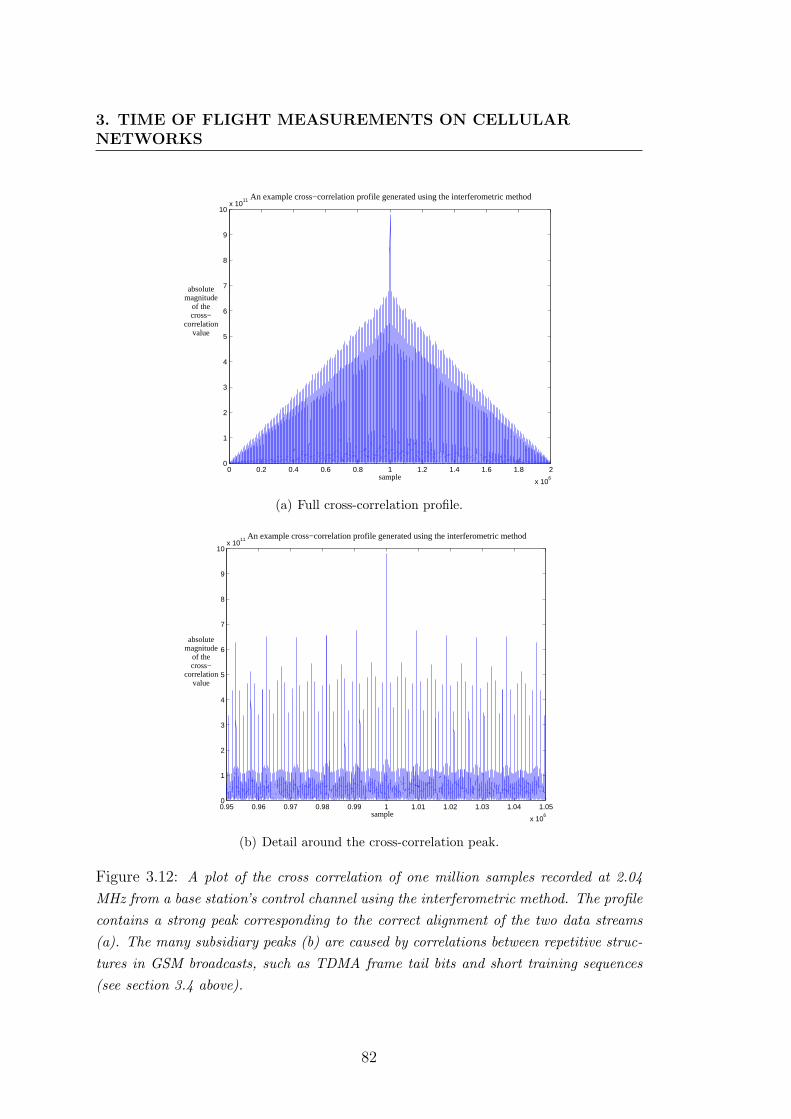
3. TIME OF FLIGHT MEASUREMENTS ON CELLULARNETWORKS
0 0.2 0.4 0.6 0.8 1 1.2 1.4 1.6 1.8 2
x 106
0
1
2
3
4
5
6
7
8
9
10x 10
11
absolutemagnitude
of thecross−
correlationvalue
sample
An example cross−correlation profile generated using the interferometric method
(a) Full cross-correlation profile.
0.95 0.96 0.97 0.98 0.99 1 1.01 1.02 1.03 1.04 1.05
x 106
0
1
2
3
4
5
6
7
8
9
10x 10
11
absolutemagnitude
of thecross−
correlationvalue
sample
An example cross−correlation profile generated using the interferometric method
(b) Detail around the cross-correlation peak.
Figure 3.12: A plot of the cross correlation of one million samples recorded at 2.04MHz from a base station’s control channel using the interferometric method. The profilecontains a strong peak corresponding to the correct alignment of the two data streams(a). The many subsidiary peaks (b) are caused by correlations between repetitive struc-tures in GSM broadcasts, such as TDMA frame tail bits and short training sequences(see section 3.4 above).
82
3.6 The Experiments
0 200000 400000 600000 800000 10000000
0.5
1
1.5
2
2.5
3
3.5
4x 10
5
sample
absolutemagnitude
of thecross−
correlationvalue
An example cross correlation profile generated using the network−synchronised method
(a) Full cross-correlation profile.
1.4 1.42 1.44 1.46 1.48 1.5 1.52 1.54 1.56 1.58 1.6
x 106
0
0.5
1
1.5
2
2.5
3
3.5
x 105
sample
absolutemagnitude
of thecross−
correlationvalue
An example cross correlation profile generated using the network−synchronised method
(b) Detail around two cross-correlation peaks.
Figure 3.13: A plot of one million samples recorded at 2.04 MHz from a base station’scontrol channel cross correlated with the GSM ETS using the network-synchronisedmethod. The profile (a) contains ten strong peaks, each marking the position of asynchronisation burst in the transmission. Each frame containing an SCB is preceededby a frame containing a frequency control burst (seen here as the small gaps to the leftof each SCB peak in (b)). The fine-scale subsidiary peaks are caused by correlationsbetween the ETS and the short training sequence within each normal burst.
83
3. TIME OF FLIGHT MEASUREMENTS ON CELLULARNETWORKS
84
Chapter 4
GSM Network Stability
A series of experiments was performed to determine the temporal stability of
the received signals on two GSM networks and to determine the viability of the
network-synchronised measurement technique discussed in the previous chapter.
Several base stations were studied using a stationary outdoor antenna on the
Cavendish Laboratory roof. The variation in signal arrival times from a given
BTS were compared to an RFS over elapsed times of many hours. The results
are presented here as Allan deviation plots. Allan deviation plots were discussed
in Chapter 2.
4.1 Method and apparatus
The equipment was prepared for the network-synchronised method as described
in the previous chapter. The signal stabilities were measured using the varia-
tions in the positions of the SCB peaks with time. Measurements of the absolute
signal TOFs were not needed and so the equipment did not need to be moved
at the start and end of each experiment to record calibration data at the BTS.
This reduced the measurement errors associated with moving the experimental
apparatus since the equipment remained fixed in one place with reduced changes
in temperature, pressure, humidity, vibration, etc. A fixed omni-directional an-
tenna positioned 10 metres above the above the roof of the Cavendish Laboratory
85
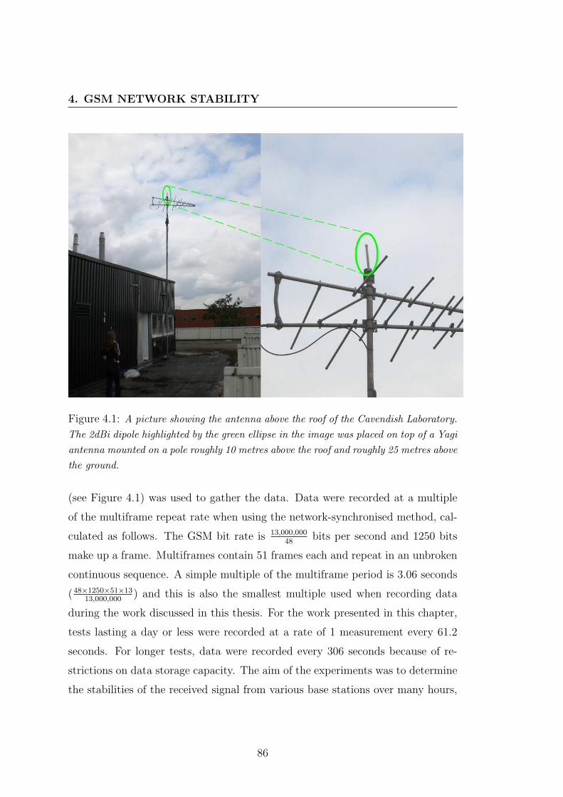
4. GSM NETWORK STABILITY
Figure 4.1: A picture showing the antenna above the roof of the Cavendish Laboratory.The 2dBi dipole highlighted by the green ellipse in the image was placed on top of a Yagiantenna mounted on a pole roughly 10 metres above the roof and roughly 25 metres abovethe ground.
(see Figure 4.1) was used to gather the data. Data were recorded at a multiple
of the multiframe repeat rate when using the network-synchronised method, cal-
culated as follows. The GSM bit rate is 13,000,00048
bits per second and 1250 bits
make up a frame. Multiframes contain 51 frames each and repeat in an unbroken
continuous sequence. A simple multiple of the multiframe period is 3.06 seconds
(48×1250×51×1313,000,000
) and this is also the smallest multiple used when recording data
during the work discussed in this thesis. For the work presented in this chapter,
tests lasting a day or less were recorded at a rate of 1 measurement every 61.2
seconds. For longer tests, data were recorded every 306 seconds because of re-
strictions on data storage capacity. The aim of the experiments was to determine
the stabilities of the received signal from various base stations over many hours,
86
4.1 Method and apparatus
and recording a measurement every few minutes was an adequate sampling period
for this purpose. Since the antenna remained stationary and in an open, high
environment, any variation in the SCB peak position was expected to be caused
by (i) measurement noise, (ii) the stability of the BTS’s transmitting equipment
and frequency reference, (iii) the stability of the signal’s propagation path, and
(iv) the stability of the RFS.
4.1.1 Calibration
A Racal 6104 Digital Radio Test Set [59] (a GSM signal generator), was connected
directly to the digitiser’s input with a short cable and phase-locked to an FRK-H
Rubidium oscillator identical to the one being used as the frequency reference by
the measurement apparatus (see Figure 4.2). The RACAL generated a BCCH
signal and the resulting Allan deviation plot is shown below as the red curve in
Figure 4.3. This red curve can be regarded as the base-line for the measurement
apparatus, as the signal was phase locked to a Rubidium atomic standard and
there was no propagation channel. The green curve in the same figure was gen-
erated with the Racal locked to its internal OCXO, with all other aspects being
the same. The curves in Figure 4.3 show that the measurement noise was the
dominant feature in the calibration data for short time scales. Both curves are
initially straight with a gradient of −1 and lie along the same line, showing that
the stabilities in these regions were dominated by random white noise on the
signal rather than by the stabilities of the frequency references (see Section 2.1
in Chapter 2). The vertical positions of these ‘-1’ regions with respect to the
axes were determined by the noise level. The signal stabilities over longer time
scales were determined by the respective stabilities of the frequency references,
as shown by the regions where the curves flatten off and the gradients become
positive.
The red curve has not been corrected for the Allan deviation of the FRK-
H used as the reference in the measurement apparatus and therefore represents
87
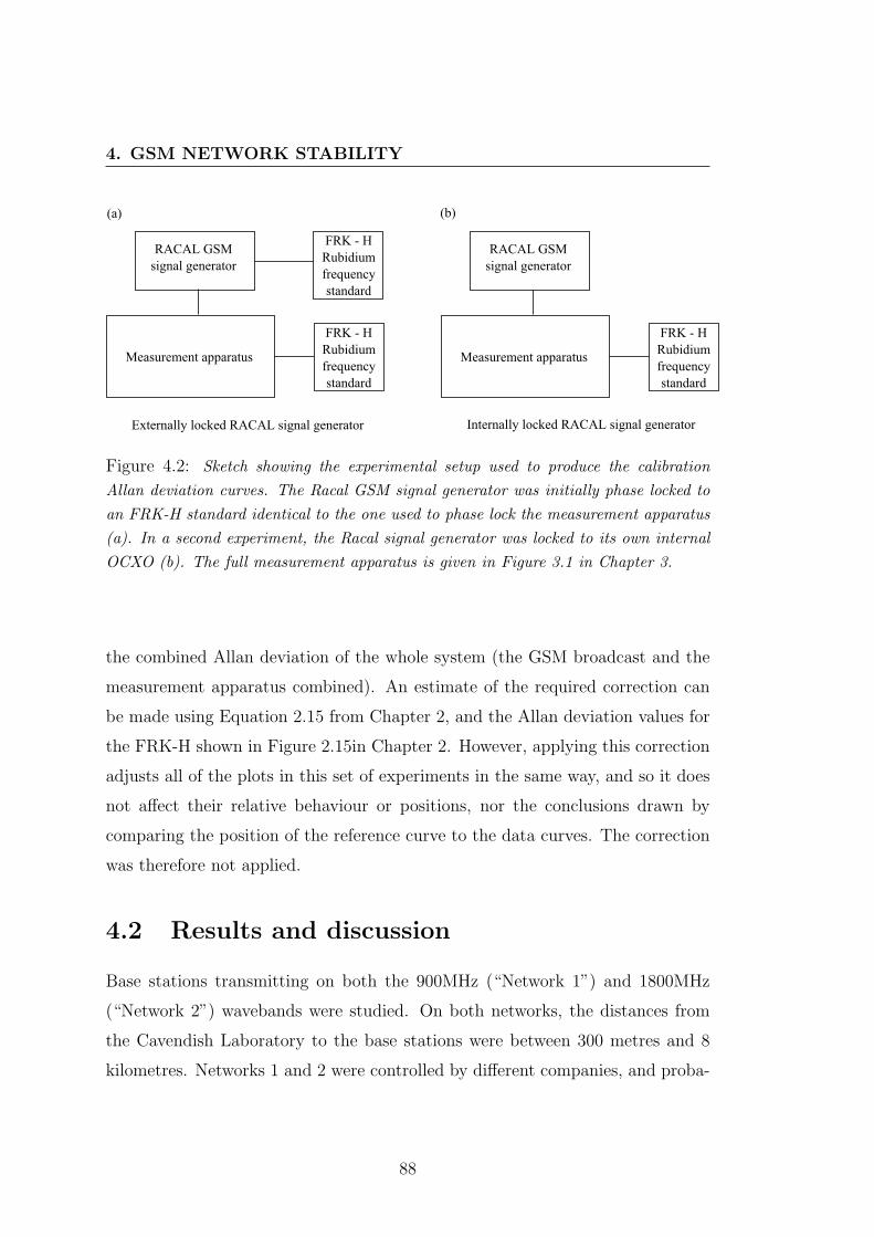
4. GSM NETWORK STABILITY
Figure 4.2: Sketch showing the experimental setup used to produce the calibrationAllan deviation curves. The Racal GSM signal generator was initially phase locked toan FRK-H standard identical to the one used to phase lock the measurement apparatus(a). In a second experiment, the Racal signal generator was locked to its own internalOCXO (b). The full measurement apparatus is given in Figure 3.1 in Chapter 3.
the combined Allan deviation of the whole system (the GSM broadcast and the
measurement apparatus combined). An estimate of the required correction can
be made using Equation 2.15 from Chapter 2, and the Allan deviation values for
the FRK-H shown in Figure 2.15in Chapter 2. However, applying this correction
adjusts all of the plots in this set of experiments in the same way, and so it does
not affect their relative behaviour or positions, nor the conclusions drawn by
comparing the position of the reference curve to the data curves. The correction
was therefore not applied.
4.2 Results and discussion
Base stations transmitting on both the 900MHz (“Network 1”) and 1800MHz
(“Network 2”) wavebands were studied. On both networks, the distances from
the Cavendish Laboratory to the base stations were between 300 metres and 8
kilometres. Networks 1 and 2 were controlled by different companies, and proba-
88
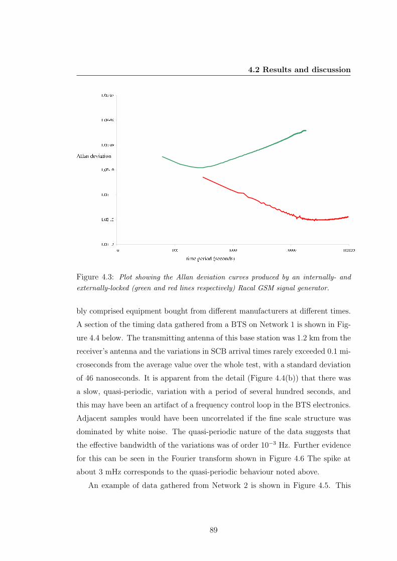
4.2 Results and discussion
Figure 4.3: Plot showing the Allan deviation curves produced by an internally- andexternally-locked (green and red lines respectively) Racal GSM signal generator.
bly comprised equipment bought from different manufacturers at different times.
A section of the timing data gathered from a BTS on Network 1 is shown in Fig-
ure 4.4 below. The transmitting antenna of this base station was 1.2 km from the
receiver’s antenna and the variations in SCB arrival times rarely exceeded 0.1 mi-
croseconds from the average value over the whole test, with a standard deviation
of 46 nanoseconds. It is apparent from the detail (Figure 4.4(b)) that there was
a slow, quasi-periodic, variation with a period of several hundred seconds, and
this may have been an artifact of a frequency control loop in the BTS electronics.
Adjacent samples would have been uncorrelated if the fine scale structure was
dominated by white noise. The quasi-periodic nature of the data suggests that
the effective bandwidth of the variations was of order 10−3 Hz. Further evidence
for this can be seen in the Fourier transform shown in Figure 4.6 The spike at
about 3 mHz corresponds to the quasi-periodic behaviour noted above.
An example of data gathered from Network 2 is shown in Figure 4.5. This
89
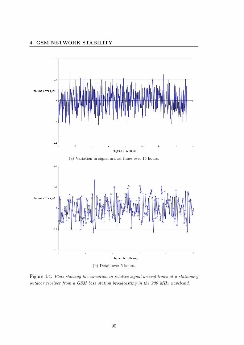
4. GSM NETWORK STABILITY
(a) Variation in signal arrival times over 15 hours.
(b) Detail over 5 hours.
Figure 4.4: Plots showing the variation in relative signal arrival times at a stationaryoutdoor receiver from a GSM base station broadcasting in the 900 MHz waveband.
90
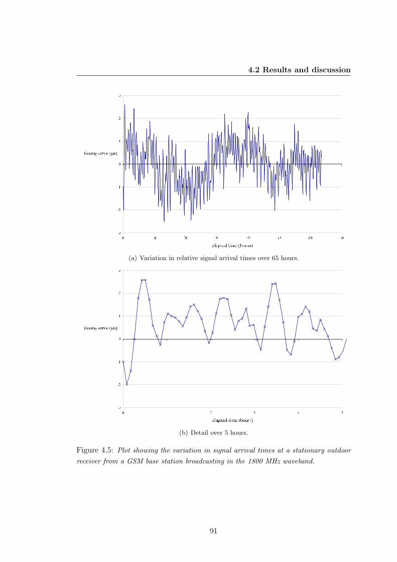
4.2 Results and discussion
(a) Variation in relative signal arrival times over 65 hours.
(b) Detail over 5 hours.
Figure 4.5: Plot showing the variation in signal arrival times at a stationary outdoorreceiver from a GSM base station broadcasting in the 1800 MHz waveband.
91
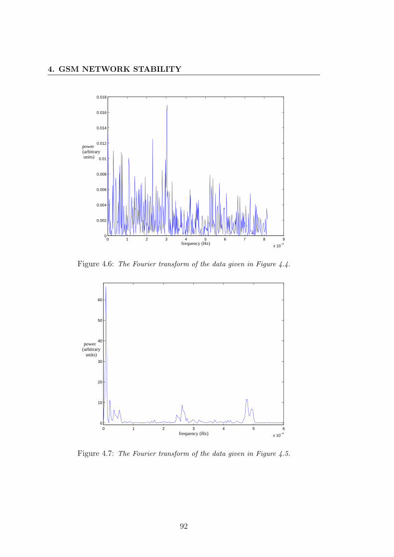
4. GSM NETWORK STABILITY
0 1 2 3 4 5 6 7 8 9
x 10−3
0
0.002
0.004
0.006
0.008
0.01
0.012
0.014
0.016
0.018
frequency (Hz)
power (arbitraryunits)
Figure 4.6: The Fourier transform of the data given in Figure 4.4.
0 1 2 3 4 5 6
x 10−4
0
10
20
30
40
50
60
frequency (Hz)
power(arbitrary
units)
Figure 4.7: The Fourier transform of the data given in Figure 4.5.
92
4.2 Results and discussion
base station was 8 km from the receiver’s antenna and appeared to be less stable
than the BTS on Network 1. The signal arrival times also show quasi-periodic
behaviour but on the longer timescale of about 40 minutes. The frequency control
loop associated with this equipment was presumably of a different design from
that of the BTS previously discussed. The slower variation on a timescale of
about 40 hours may have been caused by network control fluctuations, or effects
on the frequency reference in the base station such as temperature and pressure
changes. The standard deviation of this data set is about 0.9 microseconds. The
Fourier transform of the data is given in Figure 4.7. The large spike near the
origin corresponds to the 40-hour time variation. The quasi-periodic behaviour
with a timescale of about 40 minutes manifests itself in significant power around
0.26 and 0.48 mHz.
Variations on these timescales were not observed in the data measured on
Network 1, suggesting that they were associated with the BTS on Network 2 and
not with the measurement apparatus.
It should be noted at this point that each BTS has its own local frequency
reference, which under GSM specifications [60] has to maintain a frequency ac-
curacy (corresponding to the bias error discussed in Chapter 2) of 5× 10⁻⁸. The
most common method of maintaining this accuracy involves using the commu-
nications backbone to compare the frequency reference at the BTS to a stable
central reference which may be trained by GPS. Different manufacturers use dif-
ferent correction techniques, with some allowing the BTS to drift until a certain
threshold is reached before applying a correction, and others using a control loop.
4.2.1 900 MHz Network
Figure 4.8 shows the Allan deviation plots for four base stations on the 900MHz
network and two reference curves.
The black curve labelled ‘Ref’ represents a Racal GSM generator phase locked
to an FRK-H Rubidium oscillator (reproduced from Figure 4.3), and corresponds
93
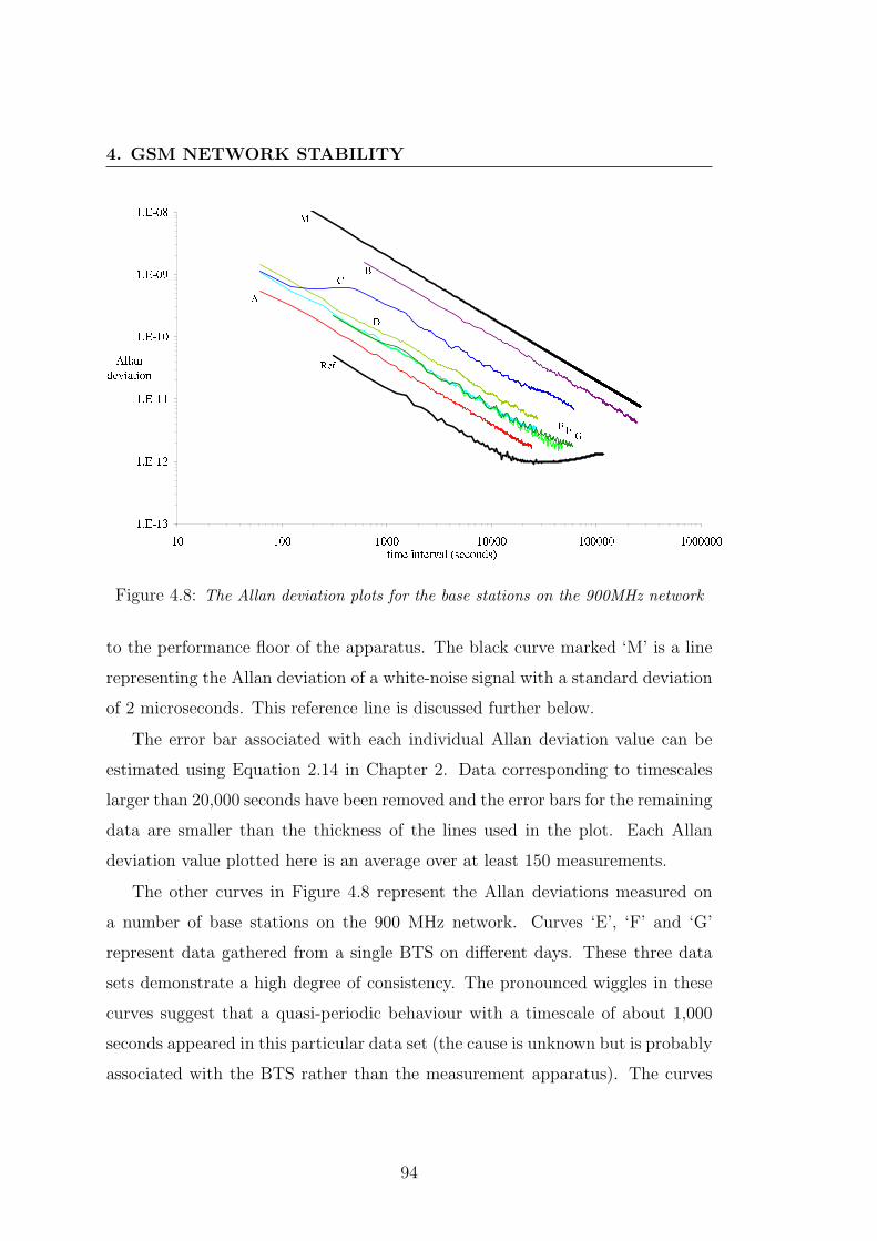
4. GSM NETWORK STABILITY
Figure 4.8: The Allan deviation plots for the base stations on the 900MHz network
to the performance floor of the apparatus. The black curve marked ‘M’ is a line
representing the Allan deviation of a white-noise signal with a standard deviation
of 2 microseconds. This reference line is discussed further below.
The error bar associated with each individual Allan deviation value can be
estimated using Equation 2.14 in Chapter 2. Data corresponding to timescales
larger than 20,000 seconds have been removed and the error bars for the remaining
data are smaller than the thickness of the lines used in the plot. Each Allan
deviation value plotted here is an average over at least 150 measurements.
The other curves in Figure 4.8 represent the Allan deviations measured on
a number of base stations on the 900 MHz network. Curves ‘E’, ‘F’ and ‘G’
represent data gathered from a single BTS on different days. These three data
sets demonstrate a high degree of consistency. The pronounced wiggles in these
curves suggest that a quasi-periodic behaviour with a timescale of about 1,000
seconds appeared in this particular data set (the cause is unknown but is probably
associated with the BTS rather than the measurement apparatus). The curves
94
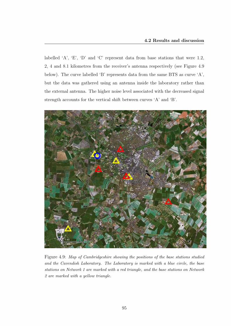
4.2 Results and discussion
labelled ‘A’, ‘E’, ‘D’ and ‘C’ represent data from base stations that were 1.2,
2, 4 and 8.1 kilometres from the receiver’s antenna respectively (see Figure 4.9
below). The curve labelled ‘B’ represents data from the same BTS as curve ‘A’,
but the data was gathered using an antenna inside the laboratory rather than
the external antenna. The higher noise level associated with the decreased signal
strength accounts for the vertical shift between curves ‘A’ and ‘B’.
Figure 4.9: Map of Cambridgeshire showing the positions of the base stations studiedand the Cavendish Laboratory. The Laboratory is marked with a blue circle, the basestations on Network 1 are marked with a red triangle, and the base stations on Network2 are marked with a yellow triangle.
95
4. GSM NETWORK STABILITY
Curves ‘A’ to ‘G’ do not come close enough to the reference curve (‘Ref’)
to be affected by the behaviour of the RFS. All of the curves show that the
base stations studied on Network 1 were highly stable and that their frequency
references were approaching the stability of the FRK-H atomic reference. This
suggests that the crystal oscillators in the BTSs were locked to a central network
frequency reference of high stability using an underlying network-wide stabilising
mechanism as mentioned above. It also suggests that the network-synchronised
method discussed in the previous chapter will be as accurate as the interferometric
method when studying these base stations.
Curve ‘C’ exhibits a deviation from its initial −1 gradient over time periods
of 100–600 seconds before settling back to a −1 gradient. This is not typical for
a free running oscillator (see Section 2.1 in Chapter 2). This behaviour can how-
ever be caused by a perturbation with a characteristic timescale superimposed
on an otherwise highly stable signal. The variation is not an oscillation with a
fixed frequency, as this would result in a oscillation on the Allan deviation plot
marking out the period and sub-harmonics of the oscillation. Figure 4.10 shows
the sampled data gathered from this BTS and it can be clearly seen that there is
both a fine scale regular structure showing variations of around 1.5 microseconds
over roughly 20 minutes, and a smooth wander of a microsecond over timescales
of around 10 hours or more. Comparing these time periods to the Allan devi-
ation plot, the fine scale structure is responsible for the unexpected deviation
between 100 and 600 seconds. The BTS represented by curve ‘C’ was the oldest
base station studied on Network 1. The short term perturbations and long term
wander evident in Figure 4.10 are not seen in the other data sets for this network,
suggesting that this base station is not locked to a highly stable oscillator like the
newer transmitters on that network. The fact that the signal from this old BTS is
still highly stable over long time periods does however suggest that there is some
degree of frequency correction or control in operation. The finer-scale structure
is similar to the structure seen in the data from Network 2 in Figure 4.5 and may
be a feature of older base station technology. An Allan deviation plot generated
96
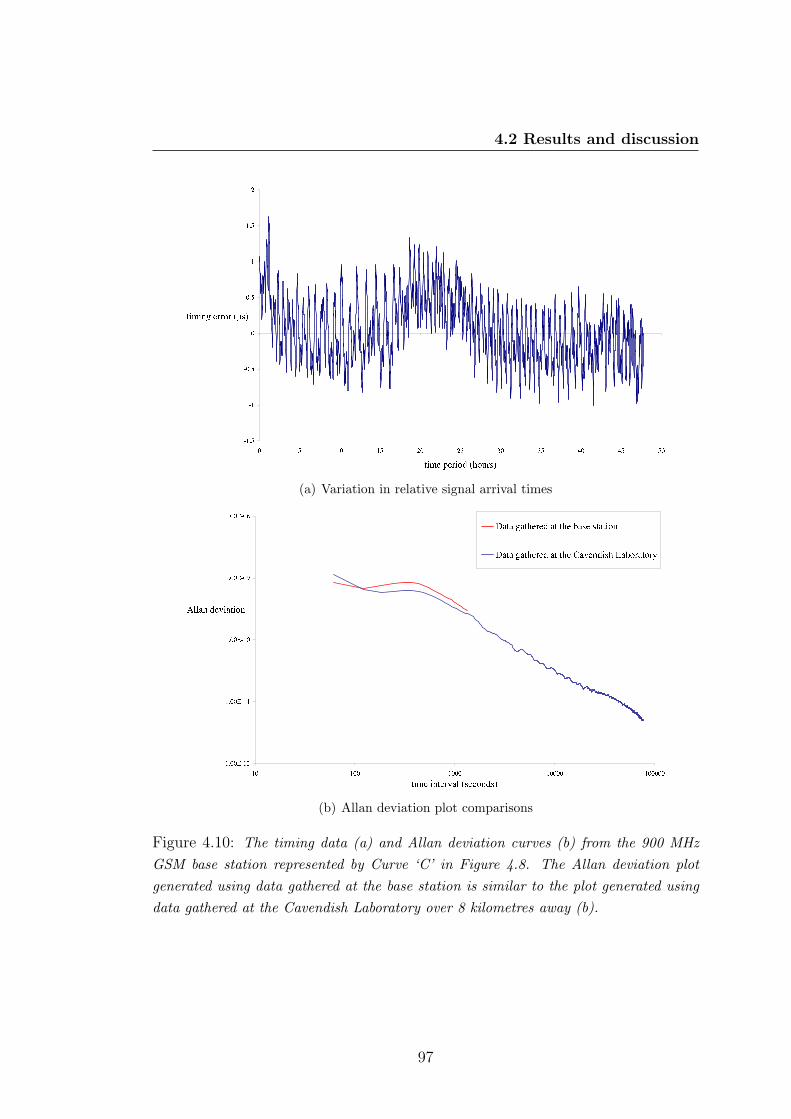
4.2 Results and discussion
(a) Variation in relative signal arrival times
(b) Allan deviation plot comparisons
Figure 4.10: The timing data (a) and Allan deviation curves (b) from the 900 MHzGSM base station represented by Curve ‘C’ in Figure 4.8. The Allan deviation plotgenerated using data gathered at the base station is similar to the plot generated usingdata gathered at the Cavendish Laboratory over 8 kilometres away (b).
97
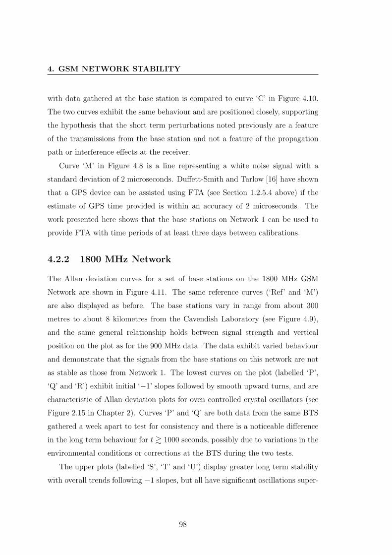
4. GSM NETWORK STABILITY
with data gathered at the base station is compared to curve ‘C’ in Figure 4.10.
The two curves exhibit the same behaviour and are positioned closely, supporting
the hypothesis that the short term perturbations noted previously are a feature
of the transmissions from the base station and not a feature of the propagation
path or interference effects at the receiver.
Curve ‘M’ in Figure 4.8 is a line representing a white noise signal with a
standard deviation of 2 microseconds. Duffett-Smith and Tarlow [16] have shown
that a GPS device can be assisted using FTA (see Section 1.2.5.4 above) if the
estimate of GPS time provided is within an accuracy of 2 microseconds. The
work presented here shows that the base stations on Network 1 can be used to
provide FTA with time periods of at least three days between calibrations.
4.2.2 1800 MHz Network
The Allan deviation curves for a set of base stations on the 1800 MHz GSM
Network are shown in Figure 4.11. The same reference curves (‘Ref’ and ‘M’)
are also displayed as before. The base stations vary in range from about 300
metres to about 8 kilometres from the Cavendish Laboratory (see Figure 4.9),
and the same general relationship holds between signal strength and vertical
position on the plot as for the 900 MHz data. The data exhibit varied behaviour
and demonstrate that the signals from the base stations on this network are not
as stable as those from Network 1. The lowest curves on the plot (labelled ‘P’,
‘Q’ and ‘R’) exhibit initial ‘−1’ slopes followed by smooth upward turns, and are
characteristic of Allan deviation plots for oven controlled crystal oscillators (see
Figure 2.15 in Chapter 2). Curves ‘P’ and ‘Q’ are both data from the same BTS
gathered a week apart to test for consistency and there is a noticeable difference
in the long term behaviour for t & 1000 seconds, possibly due to variations in the
environmental conditions or corrections at the BTS during the two tests.
The upper plots (labelled ‘S’, ‘T’ and ‘U’) display greater long term stability
with overall trends following −1 slopes, but all have significant oscillations super-
98
4.2 Results and discussion
Figure 4.11: The Allan deviation plots for the base stations on the 1800MHz network
imposed on this trend. These are caused by oscillations in the timing data (see
Figure 4.12 below) which are most likely to be a feature of the equipment and pro-
cesses used by the base stations to generate the signals rather than being caused
by propagation effects or interference. These two distinct groups of curves suggest
that there are at least two groups of base stations on Network 2: (a) those with
unregulated or infrequently-regulated crystal frequency references and (b) those
with more stable or regularly-corrected reference sources but a further source of
inherent instability producing an oscillation in the signal transmission times. The
oscillation could be caused, for example, by the BTS’s frequency reference being
strongly over-corrected each time it deviates away from its nominal frequency by
a certain amount.
The position of the curves relative to the two-microsecond line shows that this
network can be used to provide FTA, but the method can only be guaranteed for
time periods between calibrations of about 5 hours or less. Curves ‘S’ and ‘T’ are
both data from the same BTS gathered a week apart, and they are reasonably
99
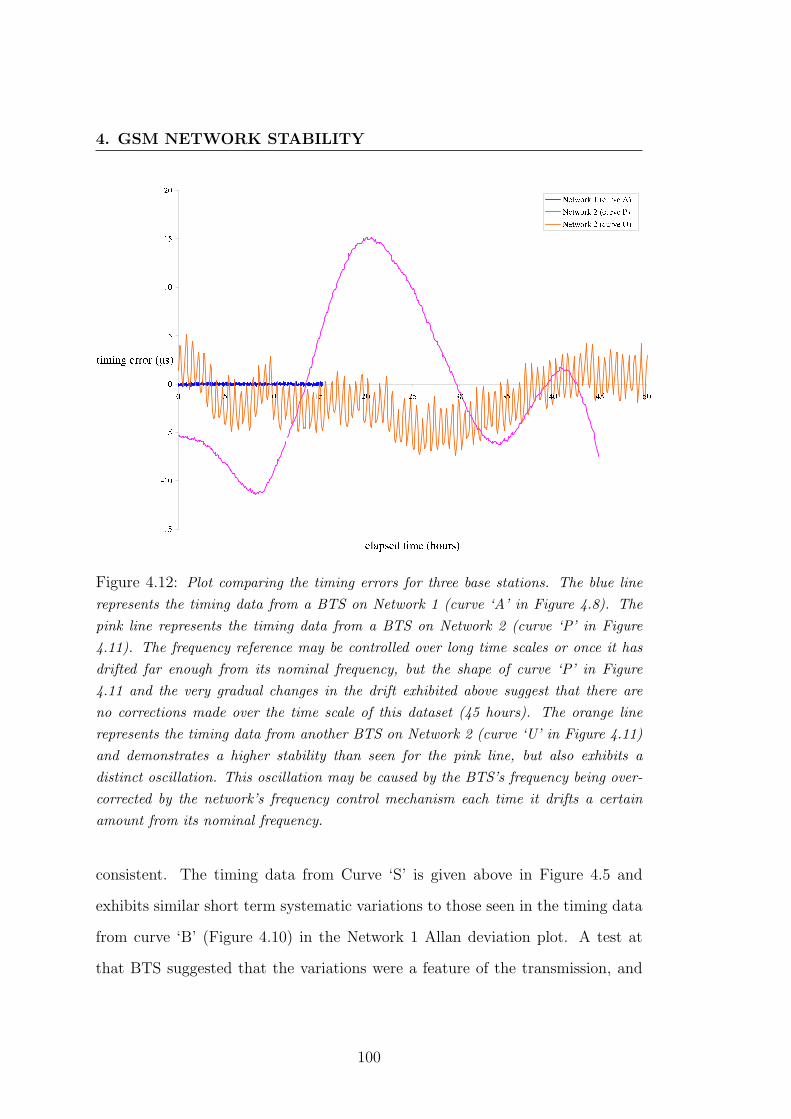
4. GSM NETWORK STABILITY
Figure 4.12: Plot comparing the timing errors for three base stations. The blue linerepresents the timing data from a BTS on Network 1 (curve ‘A’ in Figure 4.8). Thepink line represents the timing data from a BTS on Network 2 (curve ‘P’ in Figure4.11). The frequency reference may be controlled over long time scales or once it hasdrifted far enough from its nominal frequency, but the shape of curve ‘P’ in Figure4.11 and the very gradual changes in the drift exhibited above suggest that there areno corrections made over the time scale of this dataset (45 hours). The orange linerepresents the timing data from another BTS on Network 2 (curve ‘U’ in Figure 4.11)and demonstrates a higher stability than seen for the pink line, but also exhibits adistinct oscillation. This oscillation may be caused by the BTS’s frequency being over-corrected by the network’s frequency control mechanism each time it drifts a certainamount from its nominal frequency.
consistent. The timing data from Curve ‘S’ is given above in Figure 4.5 and
exhibits similar short term systematic variations to those seen in the timing data
from curve ‘B’ (Figure 4.10) in the Network 1 Allan deviation plot. A test at
that BTS suggested that the variations were a feature of the transmission, and
100
4.3 Conclusions
so may be a feature of older base-station technology.
It should be noted that if a given network uses GPS to train its central tim-
ing reference, then the whole network can be a stable repository of GPS time,
extracted using the E-GPS technique. However, if the central timing reference is
not trained by GPS, the network may gradually drift relative to GPS, degrading
its E-GPS performance.
4.3 Conclusions
1. A calibration experiment was performed to determine the Allan deviation plot
that would be measured for a base station locked to a Rubidium oscillator. This
provided a reference to compare with the BTS signal stabilities.
2. The stabilities of the signals from the four base stations studied on the 900
MHz network were all very high. The stabilities were dominated by the level
of receiver and measurement noise for the full length of the tests and were all
approaching the levels expected from atomic frequency standards. This suggests
that the base stations were all locked to highly stable frequency references, such
as GPS time, or a highly stable central frequency reference. It is unlikely that
there is an expensive atomic frequency standard in every base station on the net-
work.
3. The oldest macro cell transmitter tested on the 900 MHz network exhibited a
systematic variation in its synchronisation burst transmission times over a period
of roughly ten minutes. This variation reduced the overall stability of the sig-
nal, but the data still suggested that the base station’s frequency reference was
highly stable over the full time period of the test. A test performed at the base
station suggested that the variation was a feature of the transmission and not a
propagation or interference effect.
4. The four base stations studied on the 1800 MHz network displayed lower signal
stabilities than those on the 900 MHz network. There also appeared to be two
101
4. GSM NETWORK STABILITY
types of base stations on the 1800 MHz network - those controlled by oven con-
trolled crystal oscillators and others controlled by more stable reference sources
but with an unwanted oscillation or semi-periodic variation superimposed on the
signal reducing the stability.
5. The studies of the two networks suggest that Fine Time Aiding can be pro-
vided on Network 1 over time periods of 3 days or more and on Network 2 over
time periods of up to 5 hours.
6. The base stations on the 900 MHz network exhibiting signal timing stabilities
close to the timing stability of the FRK-H Rubidium atomic standard can be
used to perform experiments using the network-synchronised method described
in Chapter 3.
102
Chapter 5
The effects of indoor multipath
environments on timing stability
A series of experiments was performed to investigate the temporal stability of the
signals received from GSM base stations at a slowly-moving indoor antenna.
5.1 Method and apparatus
The experimental method for recording and analysing data was the same as de-
scribed in Chapter 4. A conveyor belt was added to the apparatus to move the
antenna smoothly and continuously across the measurement space at speeds rang-
ing from a millimetre per minute to a centimetre per second. The experiments
were performed on a grid marked out on a table top in three different areas -
outside on the flat roof of the Rutherford building of the Cavendish Laboratory,
inside a small fully-enclosed room on the roof itself (the Roof Laboratory), and
inside a room on the second floor of the Rutherford building (the Electronics
Laboratory).
The maximum distance sampled in each experiment was restricted by the sizes
of the desks and work surfaces available to 60–70 centimetres. Various recording
rates and conveyor belt speeds were tested in order to find a balance between
sampling as finely as possible in space to provide a high spacial resolution, and
103
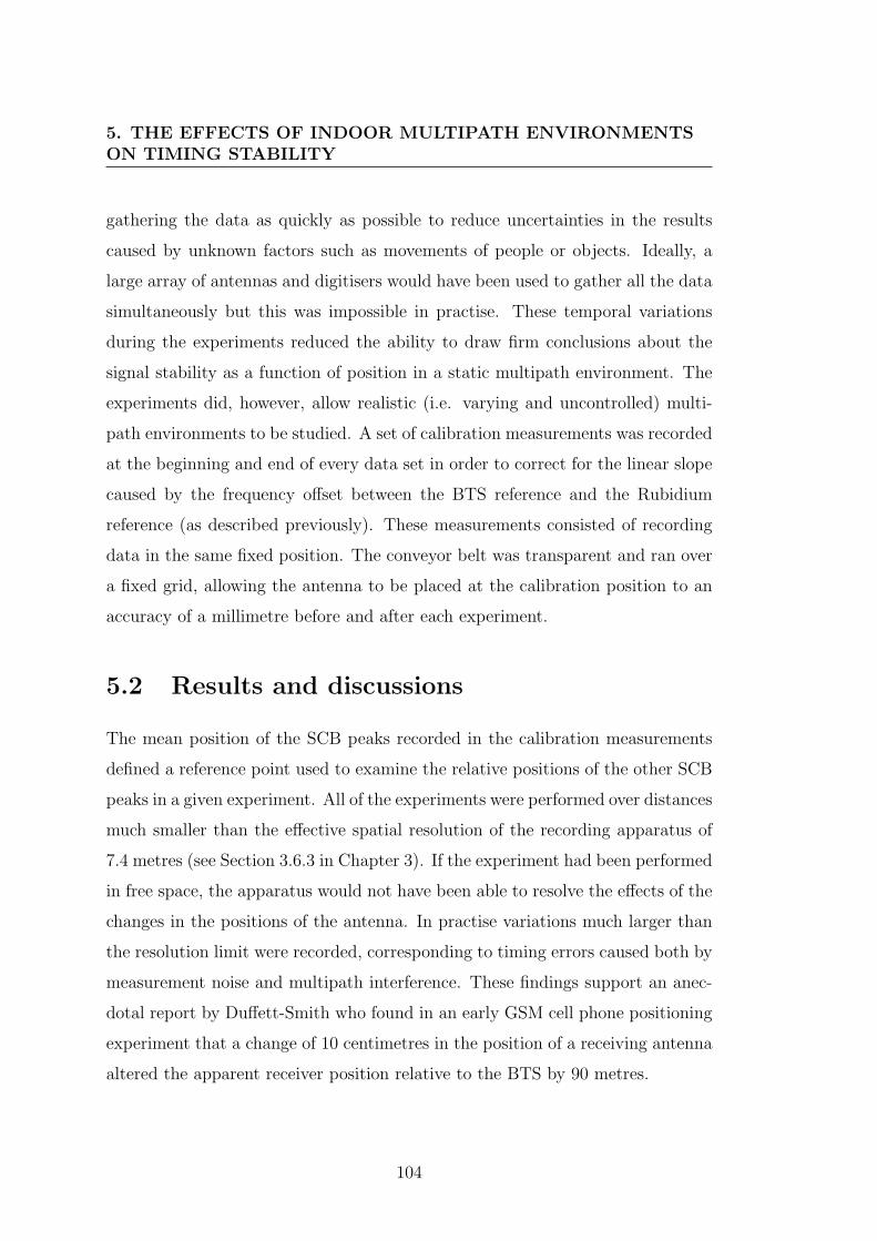
5. THE EFFECTS OF INDOOR MULTIPATH ENVIRONMENTSON TIMING STABILITY
gathering the data as quickly as possible to reduce uncertainties in the results
caused by unknown factors such as movements of people or objects. Ideally, a
large array of antennas and digitisers would have been used to gather all the data
simultaneously but this was impossible in practise. These temporal variations
during the experiments reduced the ability to draw firm conclusions about the
signal stability as a function of position in a static multipath environment. The
experiments did, however, allow realistic (i.e. varying and uncontrolled) multi-
path environments to be studied. A set of calibration measurements was recorded
at the beginning and end of every data set in order to correct for the linear slope
caused by the frequency offset between the BTS reference and the Rubidium
reference (as described previously). These measurements consisted of recording
data in the same fixed position. The conveyor belt was transparent and ran over
a fixed grid, allowing the antenna to be placed at the calibration position to an
accuracy of a millimetre before and after each experiment.
5.2 Results and discussions
The mean position of the SCB peaks recorded in the calibration measurements
defined a reference point used to examine the relative positions of the other SCB
peaks in a given experiment. All of the experiments were performed over distances
much smaller than the effective spatial resolution of the recording apparatus of
7.4 metres (see Section 3.6.3 in Chapter 3). If the experiment had been performed
in free space, the apparatus would not have been able to resolve the effects of the
changes in the positions of the antenna. In practise variations much larger than
the resolution limit were recorded, corresponding to timing errors caused both by
measurement noise and multipath interference. These findings support an anec-
dotal report by Duffett-Smith who found in an early GSM cell phone positioning
experiment that a change of 10 centimetres in the position of a receiving antenna
altered the apparent receiver position relative to the BTS by 90 metres.
104
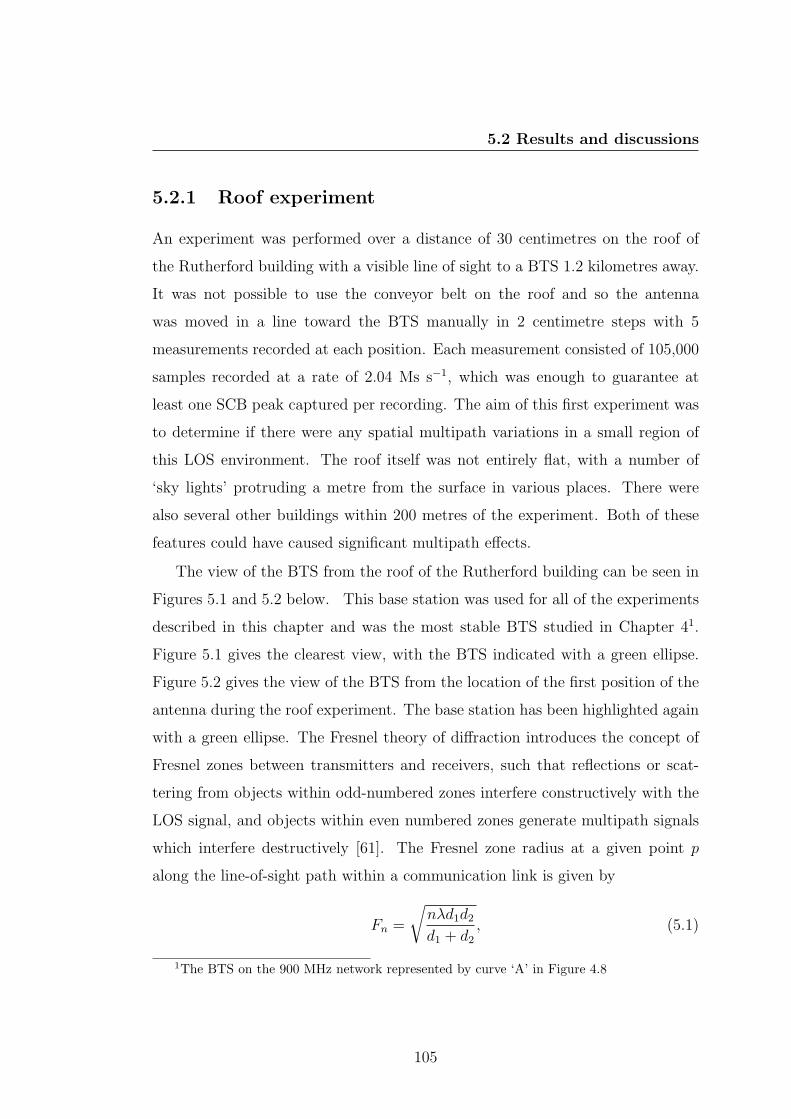
5.2 Results and discussions
5.2.1 Roof experiment
An experiment was performed over a distance of 30 centimetres on the roof of
the Rutherford building with a visible line of sight to a BTS 1.2 kilometres away.
It was not possible to use the conveyor belt on the roof and so the antenna
was moved in a line toward the BTS manually in 2 centimetre steps with 5
measurements recorded at each position. Each measurement consisted of 105,000
samples recorded at a rate of 2.04 Ms s−1, which was enough to guarantee at
least one SCB peak captured per recording. The aim of this first experiment was
to determine if there were any spatial multipath variations in a small region of
this LOS environment. The roof itself was not entirely flat, with a number of
‘sky lights’ protruding a metre from the surface in various places. There were
also several other buildings within 200 metres of the experiment. Both of these
features could have caused significant multipath effects.
The view of the BTS from the roof of the Rutherford building can be seen in
Figures 5.1 and 5.2 below. This base station was used for all of the experiments
described in this chapter and was the most stable BTS studied in Chapter 41.
Figure 5.1 gives the clearest view, with the BTS indicated with a green ellipse.
Figure 5.2 gives the view of the BTS from the location of the first position of the
antenna during the roof experiment. The base station has been highlighted again
with a green ellipse. The Fresnel theory of diffraction introduces the concept of
Fresnel zones between transmitters and receivers, such that reflections or scat-
tering from objects within odd-numbered zones interfere constructively with the
LOS signal, and objects within even numbered zones generate multipath signals
which interfere destructively [61]. The Fresnel zone radius at a given point p
along the line-of-sight path within a communication link is given by
Fn =
√nλd1d2
d1 + d2
, (5.1)
1The BTS on the 900 MHz network represented by curve ‘A’ in Figure 4.8
105
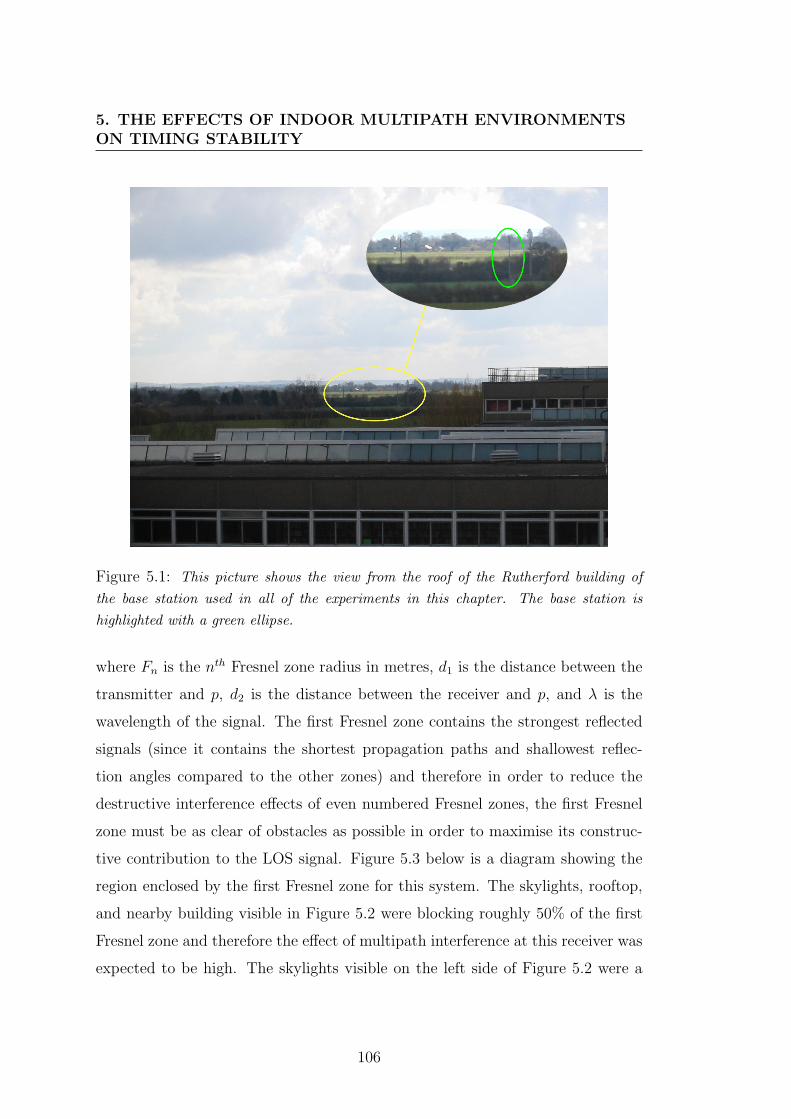
5. THE EFFECTS OF INDOOR MULTIPATH ENVIRONMENTSON TIMING STABILITY
Figure 5.1: This picture shows the view from the roof of the Rutherford building ofthe base station used in all of the experiments in this chapter. The base station ishighlighted with a green ellipse.
where Fn is the nth Fresnel zone radius in metres, d1 is the distance between the
transmitter and p, d2 is the distance between the receiver and p, and λ is the
wavelength of the signal. The first Fresnel zone contains the strongest reflected
signals (since it contains the shortest propagation paths and shallowest reflec-
tion angles compared to the other zones) and therefore in order to reduce the
destructive interference effects of even numbered Fresnel zones, the first Fresnel
zone must be as clear of obstacles as possible in order to maximise its construc-
tive contribution to the LOS signal. Figure 5.3 below is a diagram showing the
region enclosed by the first Fresnel zone for this system. The skylights, rooftop,
and nearby building visible in Figure 5.2 were blocking roughly 50% of the first
Fresnel zone and therefore the effect of multipath interference at this receiver was
expected to be high. The skylights visible on the left side of Figure 5.2 were a
106
5.2 Results and discussions
Figure 5.2: This picture shows the view of the base station from the first position ofthe antenna during the initial experiment on the roof of the Rutherford building. It ishighlighted with a green ellipse.
metre high and are just off the bottom of the picture in Figure 5.1.
The data from this experiment is shown in Figure 5.4 below. Each point on the
plot is the average SCB position of the 5 values recorded at each antenna position.
The error bars on each point are given by the standard deviation of each set of
5 values and they give an estimate of the measurement noise for the experiment.
The large timing error recorded 10 centimetres from the starting position suggests
that the antenna was moved 450 metres toward the base station. The standard
deviation of the 5 samples recorded at this position is only 75 metres, and so
measurement noise alone could not account for such a large error. These five
measurements were recorded over 30 consecutive seconds, suggesting that this
anomaly was present over at least half a minute. As shown later, this apparent
shift in position was caused by the effects of multipath interference distorting
107
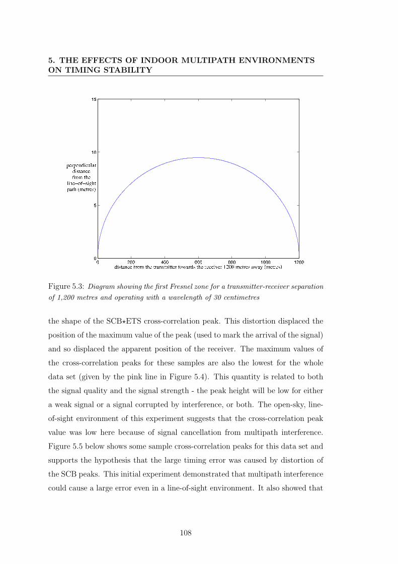
5. THE EFFECTS OF INDOOR MULTIPATH ENVIRONMENTSON TIMING STABILITY
Figure 5.3: Diagram showing the first Fresnel zone for a transmitter-receiver separationof 1,200 metres and operating with a wavelength of 30 centimetres
the shape of the SCB?ETS cross-correlation peak. This distortion displaced the
position of the maximum value of the peak (used to mark the arrival of the signal)
and so displaced the apparent position of the receiver. The maximum values of
the cross-correlation peaks for these samples are also the lowest for the whole
data set (given by the pink line in Figure 5.4). This quantity is related to both
the signal quality and the signal strength - the peak height will be low for either
a weak signal or a signal corrupted by interference, or both. The open-sky, line-
of-sight environment of this experiment suggests that the cross-correlation peak
value was low here because of signal cancellation from multipath interference.
Figure 5.5 below shows some sample cross-correlation peaks for this data set and
supports the hypothesis that the large timing error was caused by distortion of
the SCB peaks. This initial experiment demonstrated that multipath interference
could cause a large error even in a line-of-sight environment. It also showed that
108
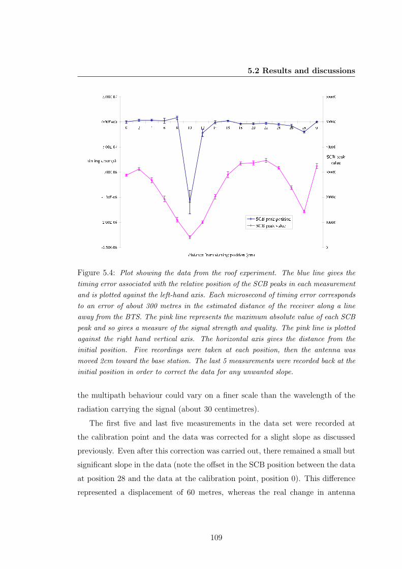
5.2 Results and discussions
Figure 5.4: Plot showing the data from the roof experiment. The blue line gives thetiming error associated with the relative position of the SCB peaks in each measurementand is plotted against the left-hand axis. Each microsecond of timing error correspondsto an error of about 300 metres in the estimated distance of the receiver along a lineaway from the BTS. The pink line represents the maximum absolute value of each SCBpeak and so gives a measure of the signal strength and quality. The pink line is plottedagainst the right hand vertical axis. The horizontal axis gives the distance from theinitial position. Five recordings were taken at each position, then the antenna wasmoved 2cm toward the base station. The last 5 measurements were recorded back at theinitial position in order to correct the data for any unwanted slope.
the multipath behaviour could vary on a finer scale than the wavelength of the
radiation carrying the signal (about 30 centimetres).
The first five and last five measurements in the data set were recorded at
the calibration point and the data was corrected for a slight slope as discussed
previously. Even after this correction was carried out, there remained a small but
significant slope in the data (note the offset in the SCB position between the data
at position 28 and the data at the calibration point, position 0). This difference
represented a displacement of 60 metres, whereas the real change in antenna
109
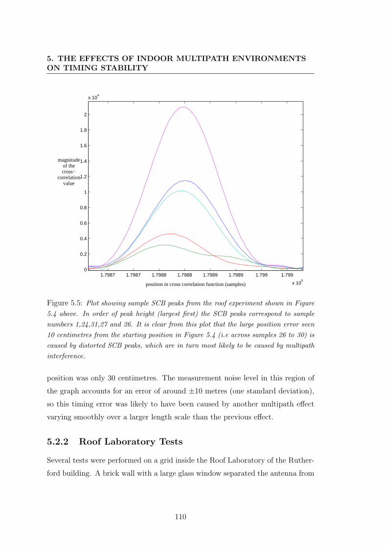
5. THE EFFECTS OF INDOOR MULTIPATH ENVIRONMENTSON TIMING STABILITY
1.7987 1.7987 1.7988 1.7988 1.7989 1.7989 1.799 1.799
x 105
0
0.2
0.4
0.6
0.8
1
1.2
1.4
1.6
1.8
2
x 104
position in cross correlation function (samples)
magnitudeof thecross−
correlationvalue
Figure 5.5: Plot showing sample SCB peaks from the roof experiment shown in Figure5.4 above. In order of peak height (largest first) the SCB peaks correspond to samplenumbers 1,24,31,27 and 26. It is clear from this plot that the large position error seen10 centimetres from the starting position in Figure 5.4 (i.e across samples 26 to 30) iscaused by distorted SCB peaks, which are in turn most likely to be caused by multipathinterference.
position was only 30 centimetres. The measurement noise level in this region of
the graph accounts for an error of around ±10 metres (one standard deviation),
so this timing error was likely to have been caused by another multipath effect
varying smoothly over a larger length scale than the previous effect.
5.2.2 Roof Laboratory Tests
Several tests were performed on a grid inside the Roof Laboratory of the Ruther-
ford building. A brick wall with a large glass window separated the antenna from
110
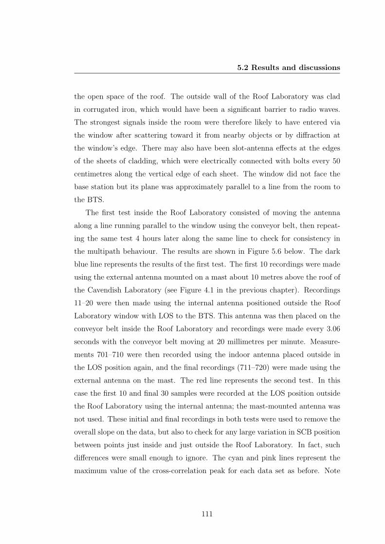
5.2 Results and discussions
the open space of the roof. The outside wall of the Roof Laboratory was clad
in corrugated iron, which would have been a significant barrier to radio waves.
The strongest signals inside the room were therefore likely to have entered via
the window after scattering toward it from nearby objects or by diffraction at
the window’s edge. There may also have been slot-antenna effects at the edges
of the sheets of cladding, which were electrically connected with bolts every 50
centimetres along the vertical edge of each sheet. The window did not face the
base station but its plane was approximately parallel to a line from the room to
the BTS.
The first test inside the Roof Laboratory consisted of moving the antenna
along a line running parallel to the window using the conveyor belt, then repeat-
ing the same test 4 hours later along the same line to check for consistency in
the multipath behaviour. The results are shown in Figure 5.6 below. The dark
blue line represents the results of the first test. The first 10 recordings were made
using the external antenna mounted on a mast about 10 metres above the roof of
the Cavendish Laboratory (see Figure 4.1 in the previous chapter). Recordings
11–20 were then made using the internal antenna positioned outside the Roof
Laboratory window with LOS to the BTS. This antenna was then placed on the
conveyor belt inside the Roof Laboratory and recordings were made every 3.06
seconds with the conveyor belt moving at 20 millimetres per minute. Measure-
ments 701–710 were then recorded using the indoor antenna placed outside in
the LOS position again, and the final recordings (711–720) were made using the
external antenna on the mast. The red line represents the second test. In this
case the first 10 and final 30 samples were recorded at the LOS position outside
the Roof Laboratory using the internal antenna; the mast-mounted antenna was
not used. These initial and final recordings in both tests were used to remove the
overall slope on the data, but also to check for any large variation in SCB position
between points just inside and just outside the Roof Laboratory. In fact, such
differences were small enough to ignore. The cyan and pink lines represent the
maximum value of the cross-correlation peak for each data set as before. Note
111
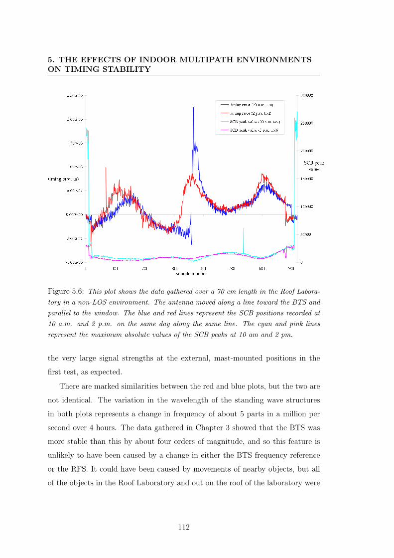
5. THE EFFECTS OF INDOOR MULTIPATH ENVIRONMENTSON TIMING STABILITY
Figure 5.6: This plot shows the data gathered over a 70 cm length in the Roof Labora-tory in a non-LOS environment. The antenna moved along a line toward the BTS andparallel to the window. The blue and red lines represent the SCB positions recorded at10 a.m. and 2 p.m. on the same day along the same line. The cyan and pink linesrepresent the maximum absolute values of the SCB peaks at 10 am and 2 pm.
the very large signal strengths at the external, mast-mounted positions in the
first test, as expected.
There are marked similarities between the red and blue plots, but the two are
not identical. The variation in the wavelength of the standing wave structures
in both plots represents a change in frequency of about 5 parts in a million per
second over 4 hours. The data gathered in Chapter 3 showed that the BTS was
more stable than this by about four orders of magnitude, and so this feature is
unlikely to have been caused by a change in either the BTS frequency reference
or the RFS. It could have been caused by movements of nearby objects, but all
of the objects in the Roof Laboratory and out on the roof of the laboratory were
112
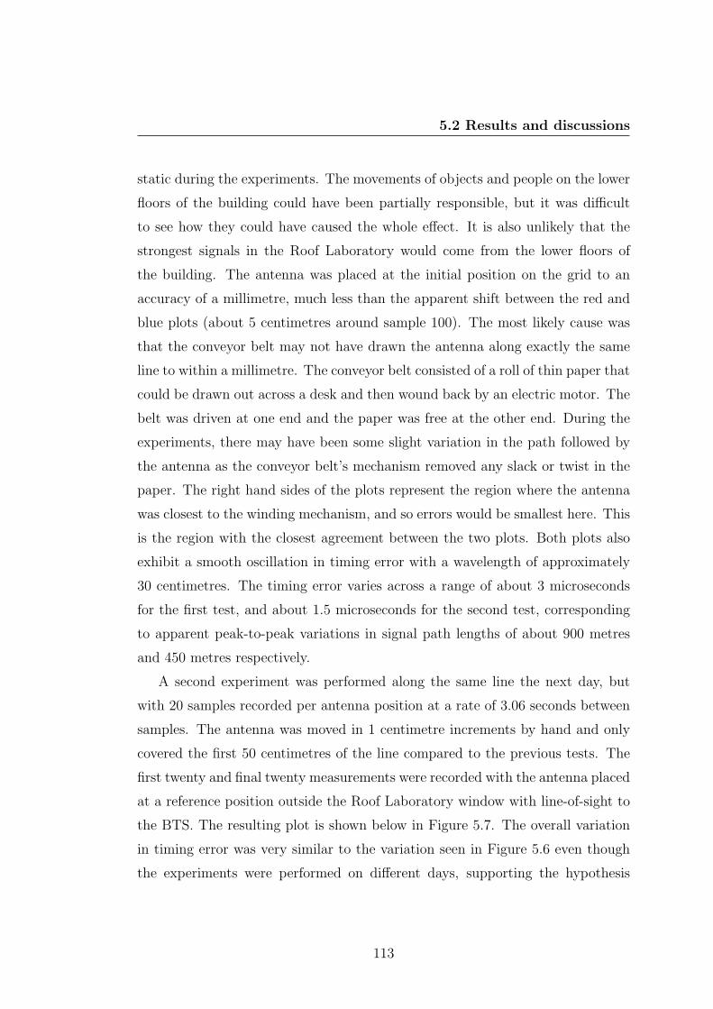
5.2 Results and discussions
static during the experiments. The movements of objects and people on the lower
floors of the building could have been partially responsible, but it was difficult
to see how they could have caused the whole effect. It is also unlikely that the
strongest signals in the Roof Laboratory would come from the lower floors of
the building. The antenna was placed at the initial position on the grid to an
accuracy of a millimetre, much less than the apparent shift between the red and
blue plots (about 5 centimetres around sample 100). The most likely cause was
that the conveyor belt may not have drawn the antenna along exactly the same
line to within a millimetre. The conveyor belt consisted of a roll of thin paper that
could be drawn out across a desk and then wound back by an electric motor. The
belt was driven at one end and the paper was free at the other end. During the
experiments, there may have been some slight variation in the path followed by
the antenna as the conveyor belt’s mechanism removed any slack or twist in the
paper. The right hand sides of the plots represent the region where the antenna
was closest to the winding mechanism, and so errors would be smallest here. This
is the region with the closest agreement between the two plots. Both plots also
exhibit a smooth oscillation in timing error with a wavelength of approximately
30 centimetres. The timing error varies across a range of about 3 microseconds
for the first test, and about 1.5 microseconds for the second test, corresponding
to apparent peak-to-peak variations in signal path lengths of about 900 metres
and 450 metres respectively.
A second experiment was performed along the same line the next day, but
with 20 samples recorded per antenna position at a rate of 3.06 seconds between
samples. The antenna was moved in 1 centimetre increments by hand and only
covered the first 50 centimetres of the line compared to the previous tests. The
first twenty and final twenty measurements were recorded with the antenna placed
at a reference position outside the Roof Laboratory window with line-of-sight to
the BTS. The resulting plot is shown below in Figure 5.7. The overall variation
in timing error was very similar to the variation seen in Figure 5.6 even though
the experiments were performed on different days, supporting the hypothesis
113
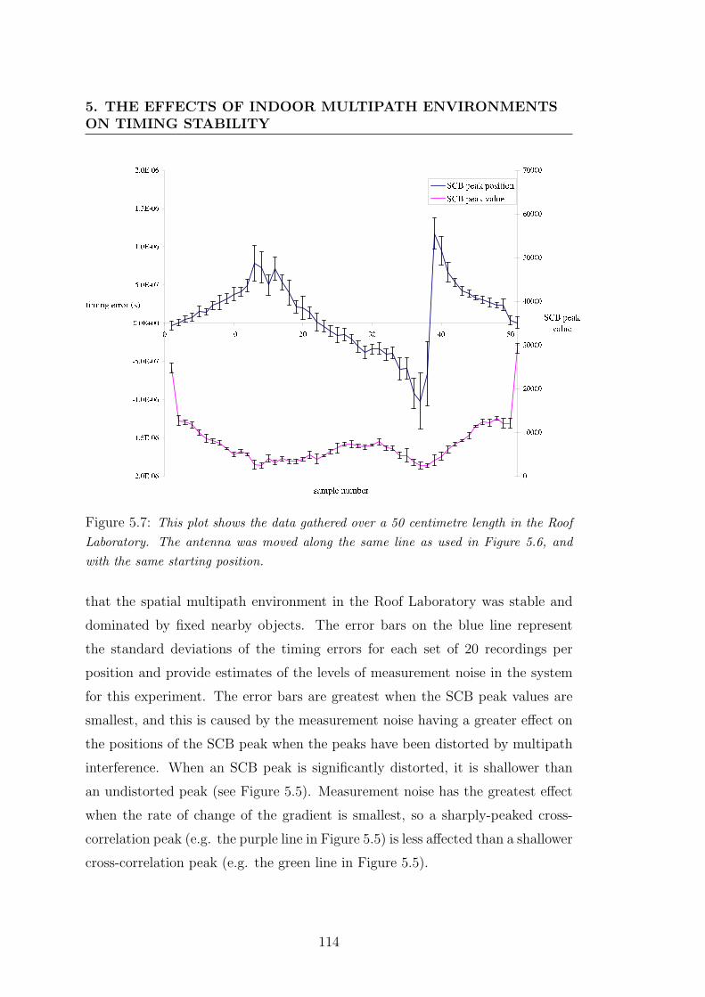
5. THE EFFECTS OF INDOOR MULTIPATH ENVIRONMENTSON TIMING STABILITY
Figure 5.7: This plot shows the data gathered over a 50 centimetre length in the RoofLaboratory. The antenna was moved along the same line as used in Figure 5.6, andwith the same starting position.
that the spatial multipath environment in the Roof Laboratory was stable and
dominated by fixed nearby objects. The error bars on the blue line represent
the standard deviations of the timing errors for each set of 20 recordings per
position and provide estimates of the levels of measurement noise in the system
for this experiment. The error bars are greatest when the SCB peak values are
smallest, and this is caused by the measurement noise having a greater effect on
the positions of the SCB peak when the peaks have been distorted by multipath
interference. When an SCB peak is significantly distorted, it is shallower than
an undistorted peak (see Figure 5.5). Measurement noise has the greatest effect
when the rate of change of the gradient is smallest, so a sharply-peaked cross-
correlation peak (e.g. the purple line in Figure 5.5) is less affected than a shallower
cross-correlation peak (e.g. the green line in Figure 5.5).
114
5.2 Results and discussions
A further experiment inside the Roof Laboratory consisted of recording data
along 5 parallel lines on the work surface, each 5 centimetres apart. The results
of the previous experiment suggested that the multipath environment had been
oversampled spatially, and so this time recordings were taken 6.12 millimetres
apart every 6.12 seconds. The results of the experiment are given below in Figure
5.8. The plot shows a number of regions with a smooth variation in timing error
Figure 5.8: This plot shows the data gathered along 5 parallel lines in the Roof Labo-ratory. Each measurement path was separated by 5 cm and the corresponding lines inthe plot have been artificially offset to allow a clear comparison of the behaviour alongand across the paths. The top line in the plot represents the path closest to the RoofLaboratory window.
over approximately 30 centimetres, as observed in the previous experiment. There
are also two discontinuous ‘double spikes’ along the yellow line. The first double
spike represents a peak-to-peak timing error of 7 microseconds, corresponding to
an uncertainty in position of 2.2 kilometres. Figure 5.9 demonstrates the cause
115
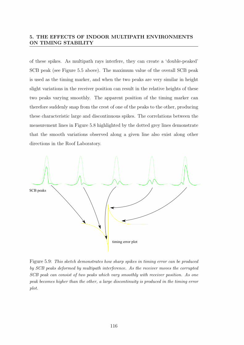
5. THE EFFECTS OF INDOOR MULTIPATH ENVIRONMENTSON TIMING STABILITY
of these spikes. As multipath rays interfere, they can create a ‘double-peaked’
SCB peak (see Figure 5.5 above). The maximum value of the overall SCB peak
is used as the timing marker, and when the two peaks are very similar in height
slight variations in the receiver position can result in the relative heights of these
two peaks varying smoothly. The apparent position of the timing marker can
therefore suddenly snap from the crest of one of the peaks to the other, producing
these characteristic large and discontinuous spikes. The correlations between the
measurement lines in Figure 5.8 highlighted by the dotted grey lines demonstrate
that the smooth variations observed along a given line also exist along other
directions in the Roof Laboratory.
Figure 5.9: This sketch demonstrates how sharp spikes in timing error can be producedby SCB peaks deformed by multipath interference. As the receiver moves the corruptedSCB peak can consist of two peaks which vary smoothly with receiver position. As onepeak becomes higher than the other, a large discontinuity is produced in the timing errorplot.
116
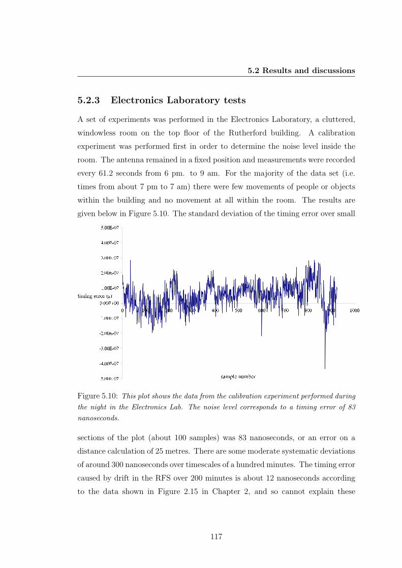
5.2 Results and discussions
5.2.3 Electronics Laboratory tests
A set of experiments was performed in the Electronics Laboratory, a cluttered,
windowless room on the top floor of the Rutherford building. A calibration
experiment was performed first in order to determine the noise level inside the
room. The antenna remained in a fixed position and measurements were recorded
every 61.2 seconds from 6 pm. to 9 am. For the majority of the data set (i.e.
times from about 7 pm to 7 am) there were few movements of people or objects
within the building and no movement at all within the room. The results are
given below in Figure 5.10. The standard deviation of the timing error over small
Figure 5.10: This plot shows the data from the calibration experiment performed duringthe night in the Electronics Lab. The noise level corresponds to a timing error of 83nanoseconds.
sections of the plot (about 100 samples) was 83 nanoseconds, or an error on a
distance calculation of 25 metres. There are some moderate systematic deviations
of around 300 nanoseconds over timescales of a hundred minutes. The timing error
caused by drift in the RFS over 200 minutes is about 12 nanoseconds according
to the data shown in Figure 2.15 in Chapter 2, and so cannot explain these
117
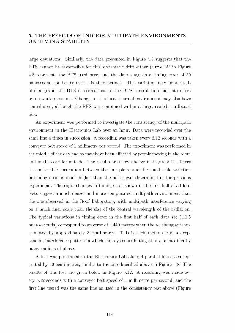
5. THE EFFECTS OF INDOOR MULTIPATH ENVIRONMENTSON TIMING STABILITY
large deviations. Similarly, the data presented in Figure 4.8 suggests that the
BTS cannot be responsible for this systematic drift either (curve ‘A’ in Figure
4.8 represents the BTS used here, and the data suggests a timing error of 50
nanoseconds or better over this time period). This variation may be a result
of changes at the BTS or corrections to the BTS control loop put into effect
by network personnel. Changes in the local thermal environment may also have
contributed, although the RFS was contained within a large, sealed, cardboard
box.
An experiment was performed to investigate the consistency of the multipath
environment in the Electronics Lab over an hour. Data were recorded over the
same line 4 times in succession. A recording was taken every 6.12 seconds with a
conveyor belt speed of 1 millimetre per second. The experiment was performed in
the middle of the day and so may have been affected by people moving in the room
and in the corridor outside. The results are shown below in Figure 5.11. There
is a noticeable correlation between the four plots, and the small-scale variation
in timing error is much higher than the noise level determined in the previous
experiment. The rapid changes in timing error shown in the first half of all four
tests suggest a much denser and more complicated multipath environment than
the one observed in the Roof Laboratory, with multipath interference varying
on a much finer scale than the size of the central wavelength of the radiation.
The typical variations in timing error in the first half of each data set (±1.5
microseconds) correspond to an error of ±440 metres when the receiving antenna
is moved by approximately 3 centimetres. This is a characteristic of a deep,
random interference pattern in which the rays contributing at any point differ by
many radians of phase.
A test was performed in the Electronics Lab along 4 parallel lines each sep-
arated by 10 centimetres, similar to the one described above in Figure 5.8. The
results of this test are given below in Figure 5.12. A recording was made ev-
ery 6.12 seconds with a conveyor belt speed of 1 millimetre per second, and the
first line tested was the same line as used in the consistency test above (Figure
118
5.2 Results and discussions
Figure 5.11: This plot shows the data from an experiment performed in the ElectronicsLaboratory. Data was recorded along the same line 4 times in succession to check forconsistency in the multipath environment over an hour. The 4 coloured lines in theupper part of the figure represent the timing errors of each test and are plotted againstthe left axis. The line with error bars in the lower part of the figure represents theaverage SCB peak maximum value at each antenna position and is plotted against theright hand axis. The error bars are given by the standard deviation of the SCB peakmaximum values recorded at each antenna position.
5.11). It should be noted, however, that the first line is not similar to the lines
generated in the consistency test. The cause for this may have been that the
two experiments were performed on different days and so different positioning or
movements of people and objects in the lab had a major effect on the multipath
environment. When comparing Figures 5.8 and 5.12 it is apparent again that the
multipath environment is much denser and more complex in the Electronics Lab
than in the Roof Laboratory. Large spikes surrounded by areas with relatively
119
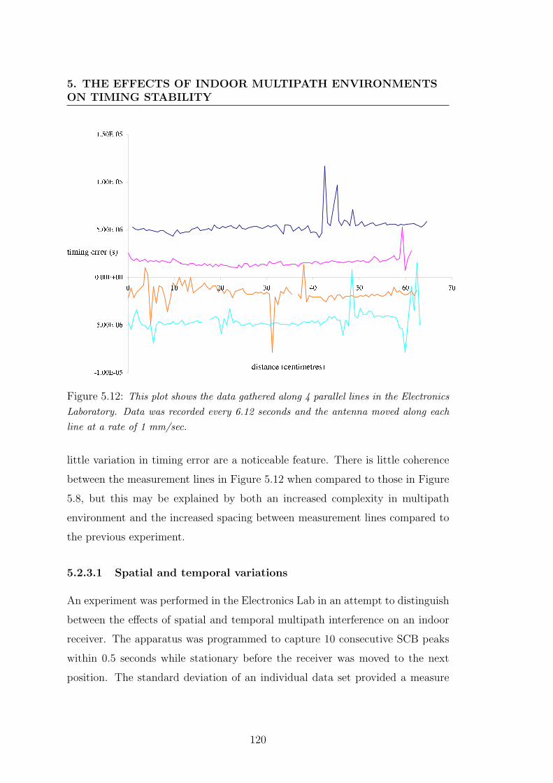
5. THE EFFECTS OF INDOOR MULTIPATH ENVIRONMENTSON TIMING STABILITY
Figure 5.12: This plot shows the data gathered along 4 parallel lines in the ElectronicsLaboratory. Data was recorded every 6.12 seconds and the antenna moved along eachline at a rate of 1 mm/sec.
little variation in timing error are a noticeable feature. There is little coherence
between the measurement lines in Figure 5.12 when compared to those in Figure
5.8, but this may be explained by both an increased complexity in multipath
environment and the increased spacing between measurement lines compared to
the previous experiment.
5.2.3.1 Spatial and temporal variations
An experiment was performed in the Electronics Lab in an attempt to distinguish
between the effects of spatial and temporal multipath interference on an indoor
receiver. The apparatus was programmed to capture 10 consecutive SCB peaks
within 0.5 seconds while stationary before the receiver was moved to the next
position. The standard deviation of an individual data set provided a measure
120
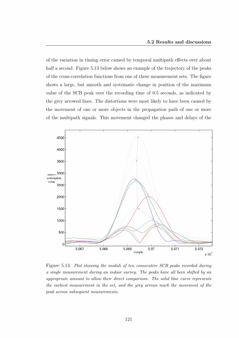
5.2 Results and discussions
of the variation in timing error caused by temporal multipath effects over about
half a second. Figure 5.13 below shows an example of the trajectory of the peaks
of the cross-correlation functions from one of these measurement sets. The figure
shows a large, but smooth and systematic change in position of the maximum
value of the SCB peak over the recording time of 0.5 seconds, as indicated by
the grey arrowed lines. The distortions were most likely to have been caused by
the movement of one or more objects in the propagation path of one or more
of the multipath signals. This movement changed the phases and delays of the
Figure 5.13: Plot showing the moduli of ten consecutive SCB peaks recorded duringa single measurement during an indoor survey. The peaks have all been shifted by anappropriate amount to allow their direct comparison. The solid blue curve representsthe earliest measurement in the set, and the grey arrows mark the movement of thepeak across subsequent measurements.
121
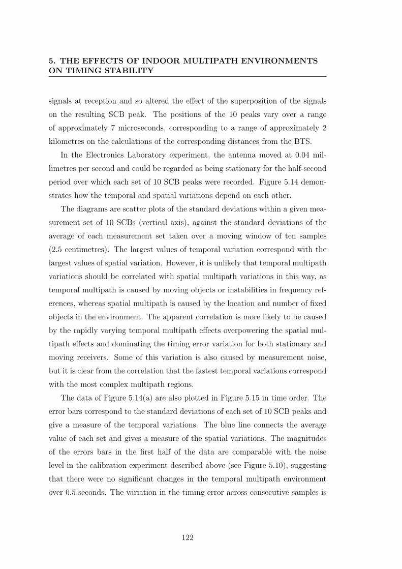
5. THE EFFECTS OF INDOOR MULTIPATH ENVIRONMENTSON TIMING STABILITY
signals at reception and so altered the effect of the superposition of the signals
on the resulting SCB peak. The positions of the 10 peaks vary over a range
of approximately 7 microseconds, corresponding to a range of approximately 2
kilometres on the calculations of the corresponding distances from the BTS.
In the Electronics Laboratory experiment, the antenna moved at 0.04 mil-
limetres per second and could be regarded as being stationary for the half-second
period over which each set of 10 SCB peaks were recorded. Figure 5.14 demon-
strates how the temporal and spatial variations depend on each other.
The diagrams are scatter plots of the standard deviations within a given mea-
surement set of 10 SCBs (vertical axis), against the standard deviations of the
average of each measurement set taken over a moving window of ten samples
(2.5 centimetres). The largest values of temporal variation correspond with the
largest values of spatial variation. However, it is unlikely that temporal multipath
variations should be correlated with spatial multipath variations in this way, as
temporal multipath is caused by moving objects or instabilities in frequency ref-
erences, whereas spatial multipath is caused by the location and number of fixed
objects in the environment. The apparent correlation is more likely to be caused
by the rapidly varying temporal multipath effects overpowering the spatial mul-
tipath effects and dominating the timing error variation for both stationary and
moving receivers. Some of this variation is also caused by measurement noise,
but it is clear from the correlation that the fastest temporal variations correspond
with the most complex multipath regions.
The data of Figure 5.14(a) are also plotted in Figure 5.15 in time order. The
error bars correspond to the standard deviations of each set of 10 SCB peaks and
give a measure of the temporal variations. The blue line connects the average
value of each set and gives a measure of the spatial variations. The magnitudes
of the errors bars in the first half of the data are comparable with the noise
level in the calibration experiment described above (see Figure 5.10), suggesting
that there were no significant changes in the temporal multipath environment
over 0.5 seconds. The variation in the timing error across consecutive samples is
122
5.2 Results and discussions
(a)
)
(b)
Figure 5.14: These scatter plots demonstrate the correlation between the timing errordue to temporal (σt) and spatial (σs) multipath variations. The upper figure (a) rep-resents the data from Figure 5.15 and lower figure (b represents the data from Figure5.16.
123
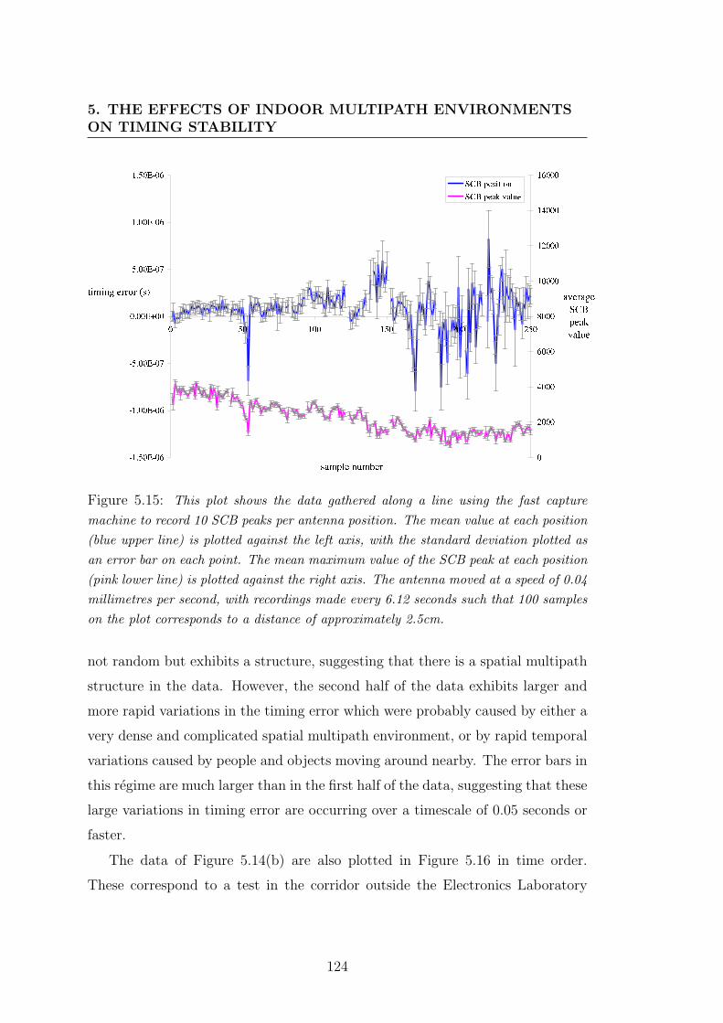
5. THE EFFECTS OF INDOOR MULTIPATH ENVIRONMENTSON TIMING STABILITY
Figure 5.15: This plot shows the data gathered along a line using the fast capturemachine to record 10 SCB peaks per antenna position. The mean value at each position(blue upper line) is plotted against the left axis, with the standard deviation plotted asan error bar on each point. The mean maximum value of the SCB peak at each position(pink lower line) is plotted against the right axis. The antenna moved at a speed of 0.04millimetres per second, with recordings made every 6.12 seconds such that 100 sampleson the plot corresponds to a distance of approximately 2.5cm.
not random but exhibits a structure, suggesting that there is a spatial multipath
structure in the data. However, the second half of the data exhibits larger and
more rapid variations in the timing error which were probably caused by either a
very dense and complicated spatial multipath environment, or by rapid temporal
variations caused by people and objects moving around nearby. The error bars in
this regime are much larger than in the first half of the data, suggesting that these
large variations in timing error are occurring over a timescale of 0.05 seconds or
faster.
The data of Figure 5.14(b) are also plotted in Figure 5.16 in time order.
These correspond to a test in the corridor outside the Electronics Laboratory
124
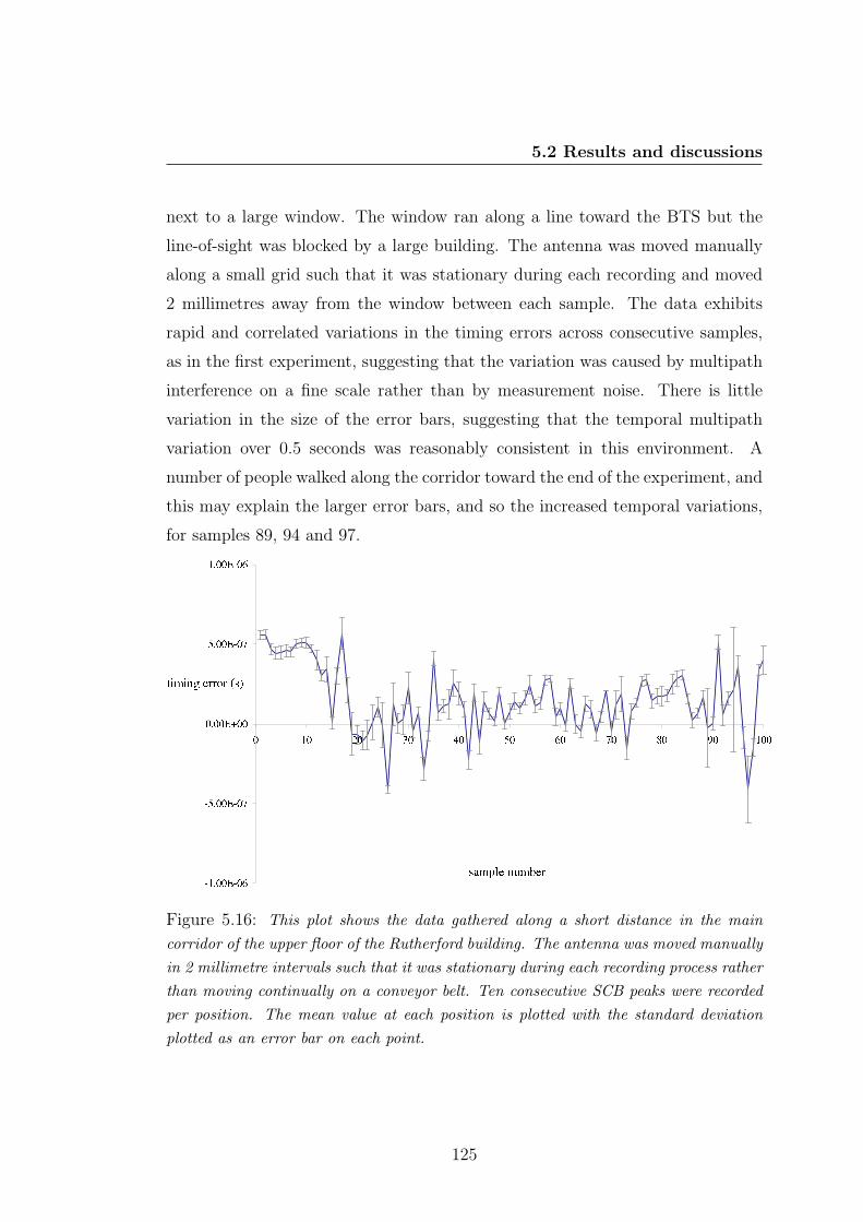
5.2 Results and discussions
next to a large window. The window ran along a line toward the BTS but the
line-of-sight was blocked by a large building. The antenna was moved manually
along a small grid such that it was stationary during each recording and moved
2 millimetres away from the window between each sample. The data exhibits
rapid and correlated variations in the timing errors across consecutive samples,
as in the first experiment, suggesting that the variation was caused by multipath
interference on a fine scale rather than by measurement noise. There is little
variation in the size of the error bars, suggesting that the temporal multipath
variation over 0.5 seconds was reasonably consistent in this environment. A
number of people walked along the corridor toward the end of the experiment, and
this may explain the larger error bars, and so the increased temporal variations,
for samples 89, 94 and 97.
Figure 5.16: This plot shows the data gathered along a short distance in the maincorridor of the upper floor of the Rutherford building. The antenna was moved manuallyin 2 millimetre intervals such that it was stationary during each recording process ratherthan moving continually on a conveyor belt. Ten consecutive SCB peaks were recordedper position. The mean value at each position is plotted with the standard deviationplotted as an error bar on each point.
125
5. THE EFFECTS OF INDOOR MULTIPATH ENVIRONMENTSON TIMING STABILITY
5.3 Conclusions
1. Significant timing errors (greater than a microsecond) can be measured in all
environment types - indoors and outdoors, and even with a line of sight to the
source. These large errors are not caused by measurement noise but by multipath
interference distorting the SCB peak.
2. These timing errors can vary over length scales much shorter than the central
wavelength of the radiation carrying the signal. Using the positions of the max-
imum absolute values of the SCB peaks as timing markers can result in errors
on position calculations as large as many kilometres, and with the error varying
with receiver position on a millimetre scale.
3. There is an apparent positive correlation between the degree of spatial and
temporal multipath interference in indoor environments, but it is more likely that
when the temporal multipath variations are large and rapidly varying they domi-
nate the overall multipath environment for both stationary and moving receivers.
126
Chapter 6
Modelling the effects of indoor
multipath environments on
timing stability
A series of simulations based on multipath interference were performed to in-
vestigate the temporal stability of the signals received from GSM base stations
at a slowly-moving indoor antenna. Three methods of measuring a GSM sig-
nal’s arrival time are also considered and compared using the simulations and
experimental data.
6.1 Modelling cross-correlation peak distortions
The experiments described in the previous chapter demonstrated that multipath
interference has a large effect on the shape of the SCB?ETS cross-correlation
peak (see Figure 5.5 above), which in turn has a large effect on the ability to use
this feature as a reliable and consistent timing reference marker. Two approaches
can be taken when modelling these distortions - a Received Signal Interference
model (RSI) and a Cross-Correlation Peak Interference model (CCPI).
127
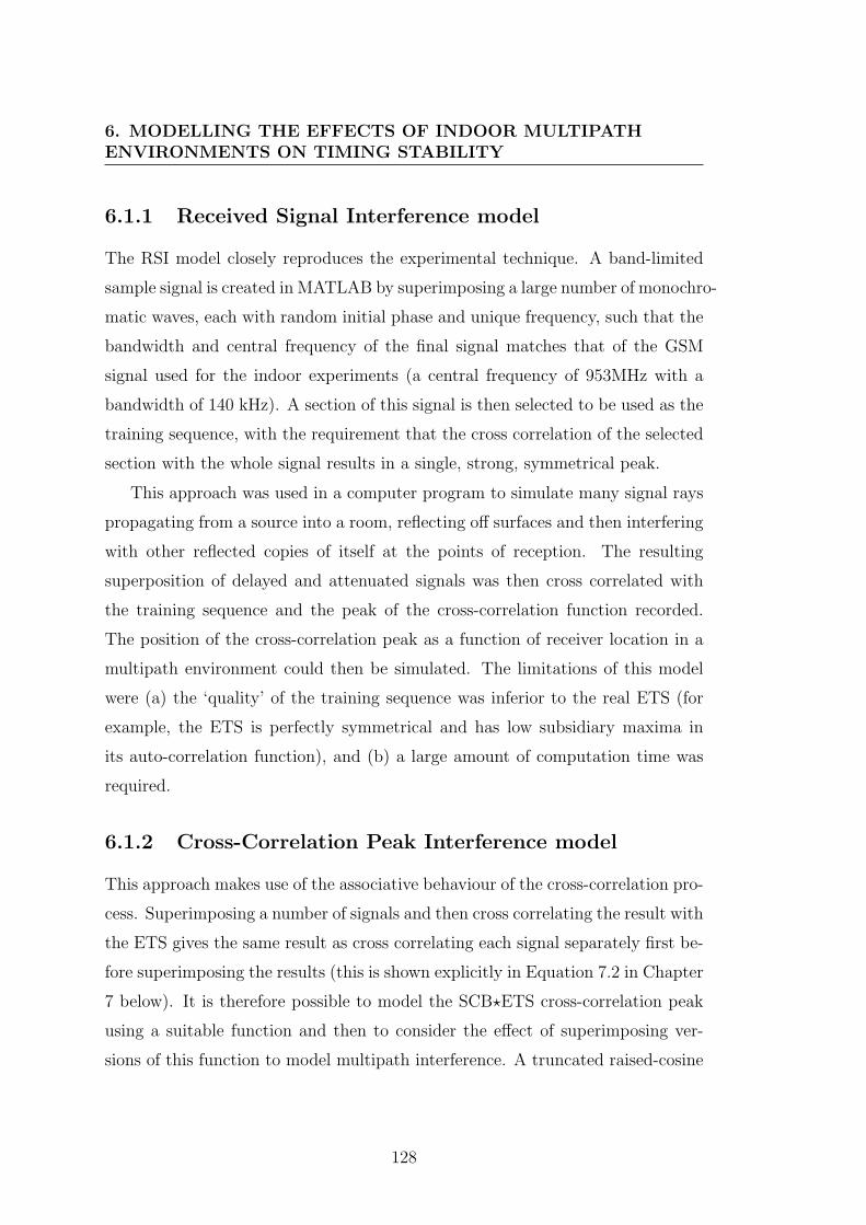
6. MODELLING THE EFFECTS OF INDOOR MULTIPATHENVIRONMENTS ON TIMING STABILITY
6.1.1 Received Signal Interference model
The RSI model closely reproduces the experimental technique. A band-limited
sample signal is created in MATLAB by superimposing a large number of monochro-
matic waves, each with random initial phase and unique frequency, such that the
bandwidth and central frequency of the final signal matches that of the GSM
signal used for the indoor experiments (a central frequency of 953MHz with a
bandwidth of 140 kHz). A section of this signal is then selected to be used as the
training sequence, with the requirement that the cross correlation of the selected
section with the whole signal results in a single, strong, symmetrical peak.
This approach was used in a computer program to simulate many signal rays
propagating from a source into a room, reflecting off surfaces and then interfering
with other reflected copies of itself at the points of reception. The resulting
superposition of delayed and attenuated signals was then cross correlated with
the training sequence and the peak of the cross-correlation function recorded.
The position of the cross-correlation peak as a function of receiver location in a
multipath environment could then be simulated. The limitations of this model
were (a) the ‘quality’ of the training sequence was inferior to the real ETS (for
example, the ETS is perfectly symmetrical and has low subsidiary maxima in
its auto-correlation function), and (b) a large amount of computation time was
required.
6.1.2 Cross-Correlation Peak Interference model
This approach makes use of the associative behaviour of the cross-correlation pro-
cess. Superimposing a number of signals and then cross correlating the result with
the ETS gives the same result as cross correlating each signal separately first be-
fore superimposing the results (this is shown explicitly in Equation 7.2 in Chapter
7 below). It is therefore possible to model the SCB?ETS cross-correlation peak
using a suitable function and then to consider the effect of superimposing ver-
sions of this function to model multipath interference. A truncated raised-cosine
128
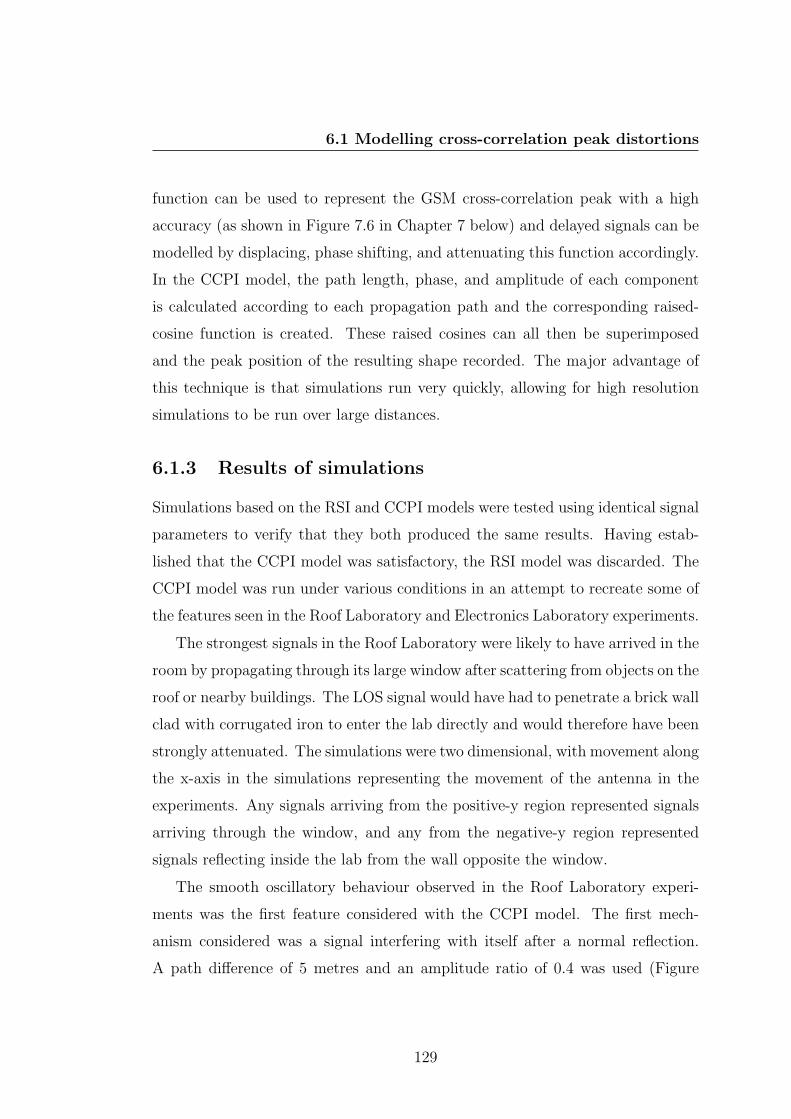
6.1 Modelling cross-correlation peak distortions
function can be used to represent the GSM cross-correlation peak with a high
accuracy (as shown in Figure 7.6 in Chapter 7 below) and delayed signals can be
modelled by displacing, phase shifting, and attenuating this function accordingly.
In the CCPI model, the path length, phase, and amplitude of each component
is calculated according to each propagation path and the corresponding raised-
cosine function is created. These raised cosines can all then be superimposed
and the peak position of the resulting shape recorded. The major advantage of
this technique is that simulations run very quickly, allowing for high resolution
simulations to be run over large distances.
6.1.3 Results of simulations
Simulations based on the RSI and CCPI models were tested using identical signal
parameters to verify that they both produced the same results. Having estab-
lished that the CCPI model was satisfactory, the RSI model was discarded. The
CCPI model was run under various conditions in an attempt to recreate some of
the features seen in the Roof Laboratory and Electronics Laboratory experiments.
The strongest signals in the Roof Laboratory were likely to have arrived in the
room by propagating through its large window after scattering from objects on the
roof or nearby buildings. The LOS signal would have had to penetrate a brick wall
clad with corrugated iron to enter the lab directly and would therefore have been
strongly attenuated. The simulations were two dimensional, with movement along
the x-axis in the simulations representing the movement of the antenna in the
experiments. Any signals arriving from the positive-y region represented signals
arriving through the window, and any from the negative-y region represented
signals reflecting inside the lab from the wall opposite the window.
The smooth oscillatory behaviour observed in the Roof Laboratory experi-
ments was the first feature considered with the CCPI model. The first mech-
anism considered was a signal interfering with itself after a normal reflection.
A path difference of 5 metres and an amplitude ratio of 0.4 was used (Figure
129
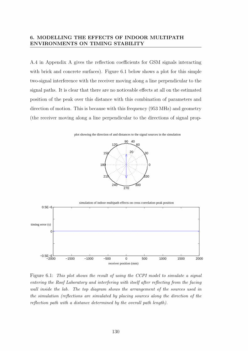
6. MODELLING THE EFFECTS OF INDOOR MULTIPATHENVIRONMENTS ON TIMING STABILITY
A.4 in Appendix A gives the reflection coefficients for GSM signals interacting
with brick and concrete surfaces). Figure 6.1 below shows a plot for this simple
two-signal interference with the receiver moving along a line perpendicular to the
signal paths. It is clear that there are no noticeable effects at all on the estimated
position of the peak over this distance with this combination of parameters and
direction of motion. This is because with this frequency (953 MHz) and geometry
(the receiver moving along a line perpendicular to the directions of signal prop-
20
40
30
210
60
240
90
270
120
300
150
330
180 0
−2000 −1500 −1000 −500 0 500 1000 1500 2000−0.5E−6
0
0.5E−6
receiver position (mm)
timing error (s)
simulation of indoor multipath effects on cross correlation peak position
plot showing the direction of and distances to the signal sources in the simulation
Figure 6.1: This plot shows the result of using the CCPI model to simulate a signalentering the Roof Laboratory and interfering with itself after reflecting from the facingwall inside the lab. The top diagram shows the arrangement of the sources used inthe simulation (reflections are simulated by placing sources along the direction of thereflection path with a distance determined by the overall path length).
130
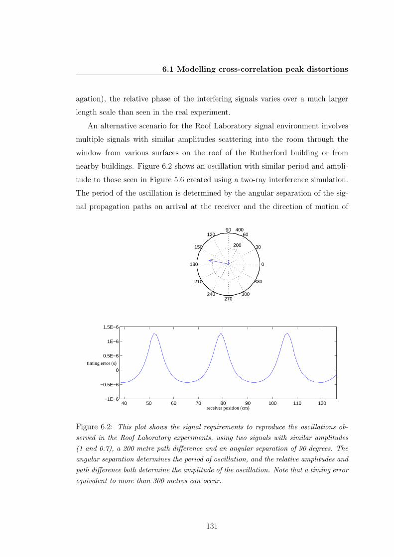
6.1 Modelling cross-correlation peak distortions
agation), the relative phase of the interfering signals varies over a much larger
length scale than seen in the real experiment.
An alternative scenario for the Roof Laboratory signal environment involves
multiple signals with similar amplitudes scattering into the room through the
window from various surfaces on the roof of the Rutherford building or from
nearby buildings. Figure 6.2 shows an oscillation with similar period and ampli-
tude to those seen in Figure 5.6 created using a two-ray interference simulation.
The period of the oscillation is determined by the angular separation of the sig-
nal propagation paths on arrival at the receiver and the direction of motion of
200
400
30
210
60
240
90
270
120
300
150
330
180 0
40 50 60 70 80 90 100 110 120−1E−6
−0.5E−6
0
0.5E−6
1E−6
1.5E−6
receiver position (cm)
timing error (s)
Figure 6.2: This plot shows the signal requirements to reproduce the oscillations ob-served in the Roof Laboratory experiments, using two signals with similar amplitudes(1 and 0.7), a 200 metre path difference and an angular separation of 90 degrees. Theangular separation determines the period of oscillation, and the relative amplitudes andpath difference both determine the amplitude of the oscillation. Note that a timing errorequivalent to more than 300 metres can occur.
131
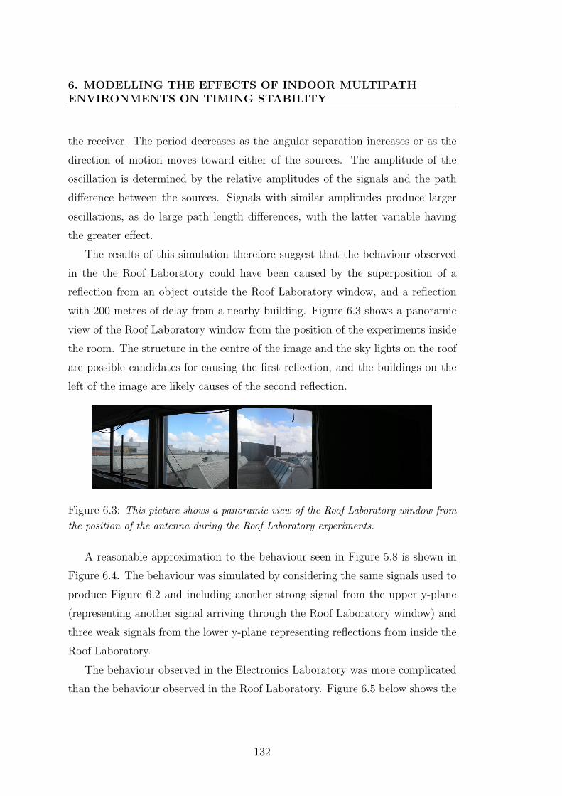
6. MODELLING THE EFFECTS OF INDOOR MULTIPATHENVIRONMENTS ON TIMING STABILITY
the receiver. The period decreases as the angular separation increases or as the
direction of motion moves toward either of the sources. The amplitude of the
oscillation is determined by the relative amplitudes of the signals and the path
difference between the sources. Signals with similar amplitudes produce larger
oscillations, as do large path length differences, with the latter variable having
the greater effect.
The results of this simulation therefore suggest that the behaviour observed
in the the Roof Laboratory could have been caused by the superposition of a
reflection from an object outside the Roof Laboratory window, and a reflection
with 200 metres of delay from a nearby building. Figure 6.3 shows a panoramic
view of the Roof Laboratory window from the position of the experiments inside
the room. The structure in the centre of the image and the sky lights on the roof
are possible candidates for causing the first reflection, and the buildings on the
left of the image are likely causes of the second reflection.
Figure 6.3: This picture shows a panoramic view of the Roof Laboratory window fromthe position of the antenna during the Roof Laboratory experiments.
A reasonable approximation to the behaviour seen in Figure 5.8 is shown in
Figure 6.4. The behaviour was simulated by considering the same signals used to
produce Figure 6.2 and including another strong signal from the upper y-plane
(representing another signal arriving through the Roof Laboratory window) and
three weak signals from the lower y-plane representing reflections from inside the
Roof Laboratory.
The behaviour observed in the Electronics Laboratory was more complicated
than the behaviour observed in the Roof Laboratory. Figure 6.5 below shows the
132
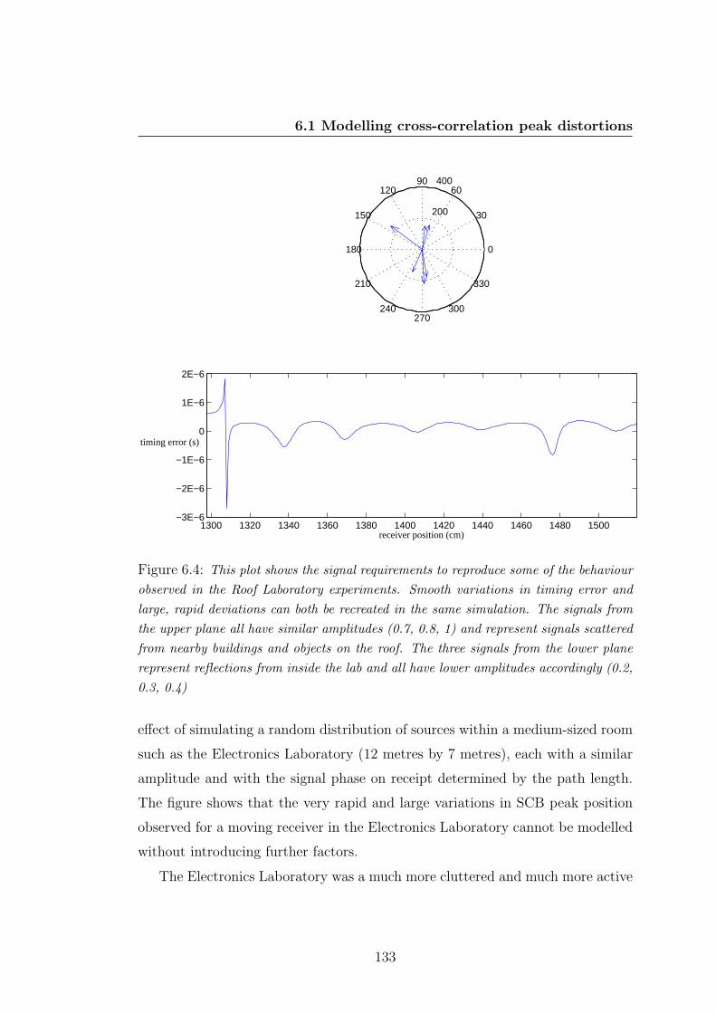
6.1 Modelling cross-correlation peak distortions
200
400
30
210
60
240
90
270
120
300
150
330
180 0
1300 1320 1340 1360 1380 1400 1420 1440 1460 1480 1500−3E−6
−2E−6
−1E−6
0
1E−6
2E−6
receiver position (cm)
timing error (s)
Figure 6.4: This plot shows the signal requirements to reproduce some of the behaviourobserved in the Roof Laboratory experiments. Smooth variations in timing error andlarge, rapid deviations can both be recreated in the same simulation. The signals fromthe upper plane all have similar amplitudes (0.7, 0.8, 1) and represent signals scatteredfrom nearby buildings and objects on the roof. The three signals from the lower planerepresent reflections from inside the lab and all have lower amplitudes accordingly (0.2,0.3, 0.4)
effect of simulating a random distribution of sources within a medium-sized room
such as the Electronics Laboratory (12 metres by 7 metres), each with a similar
amplitude and with the signal phase on receipt determined by the path length.
The figure shows that the very rapid and large variations in SCB peak position
observed for a moving receiver in the Electronics Laboratory cannot be modelled
without introducing further factors.
The Electronics Laboratory was a much more cluttered and much more active
133
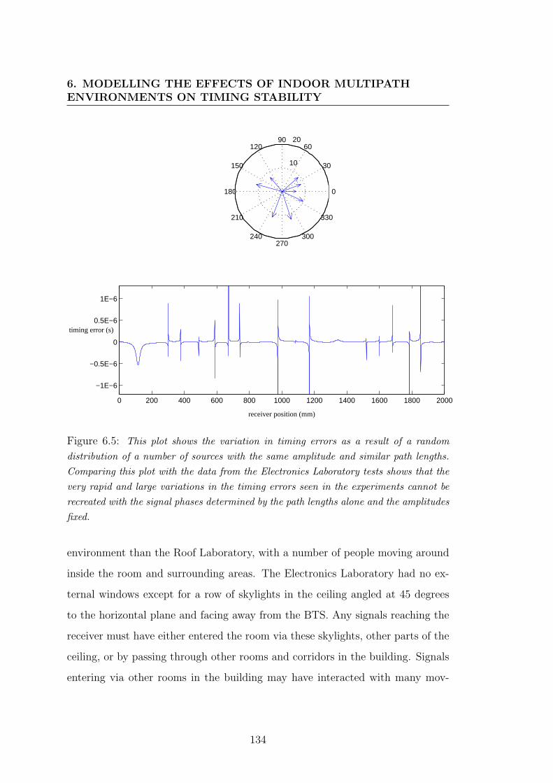
6. MODELLING THE EFFECTS OF INDOOR MULTIPATHENVIRONMENTS ON TIMING STABILITY
10
20
30
210
60
240
90
270
120
300
150
330
180 0
0 200 400 600 800 1000 1200 1400 1600 1800 2000
−1E−6
−0.5E−6
0
0.5E−6
1E−6
receiver position (mm)
timing error (s)
Figure 6.5: This plot shows the variation in timing errors as a result of a randomdistribution of a number of sources with the same amplitude and similar path lengths.Comparing this plot with the data from the Electronics Laboratory tests shows that thevery rapid and large variations in the timing errors seen in the experiments cannot berecreated with the signal phases determined by the path lengths alone and the amplitudesfixed.
environment than the Roof Laboratory, with a number of people moving around
inside the room and surrounding areas. The Electronics Laboratory had no ex-
ternal windows except for a row of skylights in the ceiling angled at 45 degrees
to the horizontal plane and facing away from the BTS. Any signals reaching the
receiver must have either entered the room via these skylights, other parts of the
ceiling, or by passing through other rooms and corridors in the building. Signals
entering via other rooms in the building may have interacted with many mov-
134
6.1 Modelling cross-correlation peak distortions
ing objects during their propagation. The movement of other objects along the
propagation path, such as tree branches, could also have produced variation in
the multipath environment measured inside the Electronics Laboratory. In order
to model these additional variations, the signals in the simulation were allocated
some random phase variation, random amplitude variation, random path length
variation, or a combination.
The phase of a 900MHz GSM signal changes over 2π radians for a movement
of around 30cm (i.e. the wavelength). Phase changes can occur on refractions,
reflections, diffractions and scattering events, and so a random phase value was
tested first to account for the movement of any people or objects interacting with
the signals before they reached the receiver.
Figure 6.6 below shows the effect of randomising the phase of each signal on
receipt. The signal amplitudes were fixed and their path lengths determined by
the coordinates of the sources and receiver. The figure shows rapid variations in
timing errors but the distribution of these variations does not accurately simulate
that observed in the experiments. The variation is relatively uniform and ran-
domising the phase effectively just increases the overall noise level on the SCB
position measurements. This method does not produce any regions with very
little variation in timing error next to regions with very large variations, which
were common features in the real experiments (see Figure 5.15 for example).
Allowing the signal path lengths and directions to vary randomly within the
range of a few metres and a few degrees respectively (to account for the movement
of people, trees, etc interacting with the propagation paths) produces very sim-
ilar results to those seen when randomising the phase as described above. This
is because these very small changes in signal delay (corresponding to roughly
0.1% of the width of the SCB peaks) are insignificant compared to the effects of
phase and amplitude variations. The random phase fluctuations resulting from
randomising the signal path lengths dominate the effect on the timing error plots
for randomised signal path lengths.
135
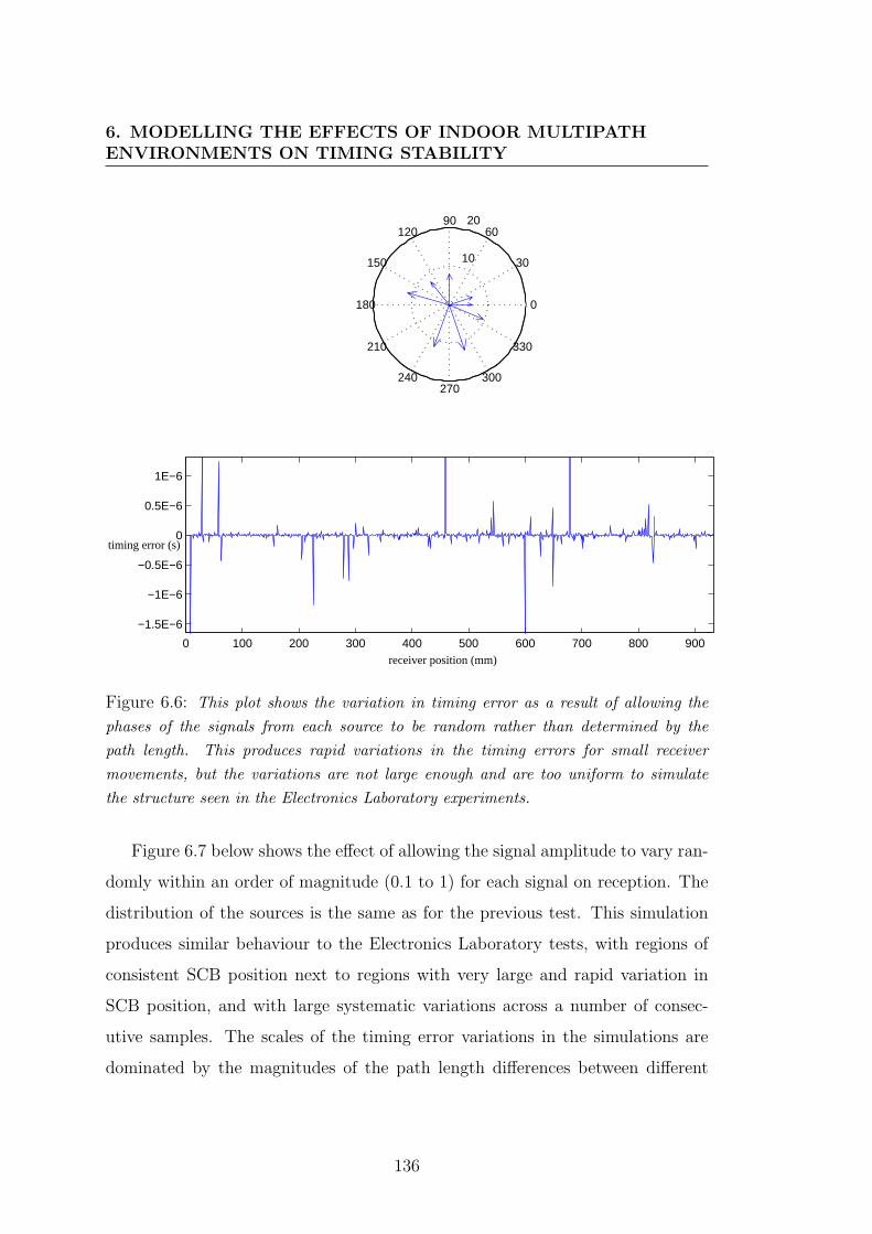
6. MODELLING THE EFFECTS OF INDOOR MULTIPATHENVIRONMENTS ON TIMING STABILITY
10
20
30
210
60
240
90
270
120
300
150
330
180 0
0 100 200 300 400 500 600 700 800 900
−1.5E−6
−1E−6
−0.5E−6
0
0.5E−6
1E−6
receiver position (mm)
timing error (s)
Figure 6.6: This plot shows the variation in timing error as a result of allowing thephases of the signals from each source to be random rather than determined by thepath length. This produces rapid variations in the timing errors for small receivermovements, but the variations are not large enough and are too uniform to simulatethe structure seen in the Electronics Laboratory experiments.
Figure 6.7 below shows the effect of allowing the signal amplitude to vary ran-
domly within an order of magnitude (0.1 to 1) for each signal on reception. The
distribution of the sources is the same as for the previous test. This simulation
produces similar behaviour to the Electronics Laboratory tests, with regions of
consistent SCB position next to regions with very large and rapid variation in
SCB position, and with large systematic variations across a number of consec-
utive samples. The scales of the timing error variations in the simulations are
dominated by the magnitudes of the path length differences between different
136
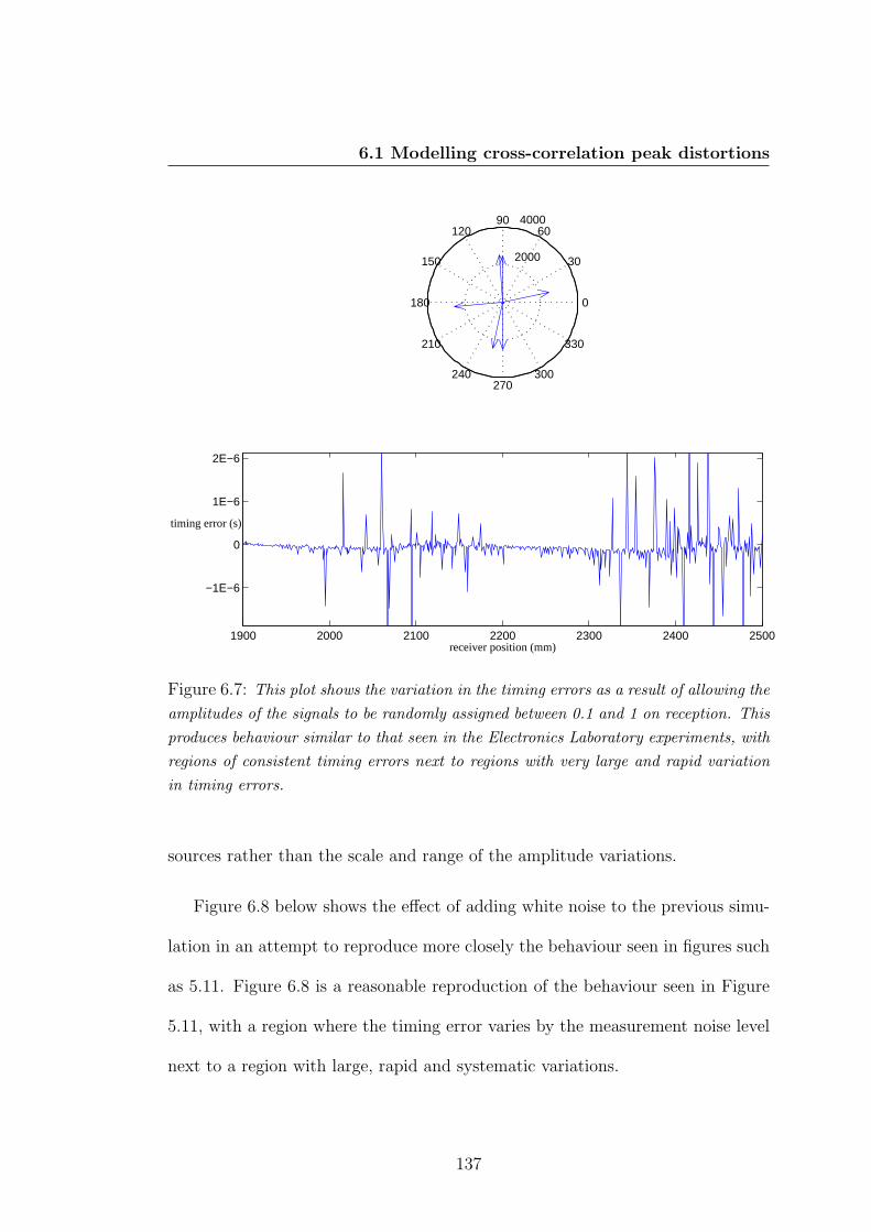
6.1 Modelling cross-correlation peak distortions
2000
4000
30
210
60
240
90
270
120
300
150
330
180 0
1900 2000 2100 2200 2300 2400 2500
−1E−6
0
1E−6
2E−6
receiver position (mm)
timing error (s)
Figure 6.7: This plot shows the variation in the timing errors as a result of allowing theamplitudes of the signals to be randomly assigned between 0.1 and 1 on reception. Thisproduces behaviour similar to that seen in the Electronics Laboratory experiments, withregions of consistent timing errors next to regions with very large and rapid variationin timing errors.
sources rather than the scale and range of the amplitude variations.
Figure 6.8 below shows the effect of adding white noise to the previous simu-
lation in an attempt to reproduce more closely the behaviour seen in figures such
as 5.11. Figure 6.8 is a reasonable reproduction of the behaviour seen in Figure
5.11, with a region where the timing error varies by the measurement noise level
next to a region with large, rapid and systematic variations.
137
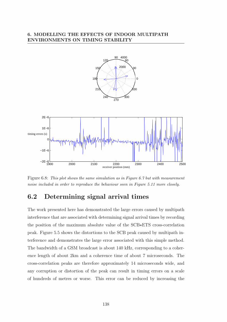
6. MODELLING THE EFFECTS OF INDOOR MULTIPATHENVIRONMENTS ON TIMING STABILITY
2000
4000
30
210
60
240
90
270
120
300
150
330
180 0
1900 2000 2100 2200 2300 2400 2500−2E−6
−1E−6
0
1E−6
2E−6
receiver position (mm)
timing errors (s)
Figure 6.8: This plot shows the same simulation as in Figure 6.7 but with measurementnoise included in order to reproduce the behaviour seen in Figure 5.11 more closely.
6.2 Determining signal arrival times
The work presented here has demonstrated the large errors caused by multipath
interference that are associated with determining signal arrival times by recording
the position of the maximum absolute value of the SCB?ETS cross-correlation
peak. Figure 5.5 shows the distortions to the SCB peak caused by multipath in-
terference and demonstrates the large error associated with this simple method.
The bandwidth of a GSM broadcast is about 140 kHz, corresponding to a coher-
ence length of about 2km and a coherence time of about 7 microseconds. The
cross-correlation peaks are therefore approximately 14 microseconds wide, and
any corruption or distortion of the peak can result in timing errors on a scale
of hundreds of metres or worse. This error can be reduced by increasing the
138
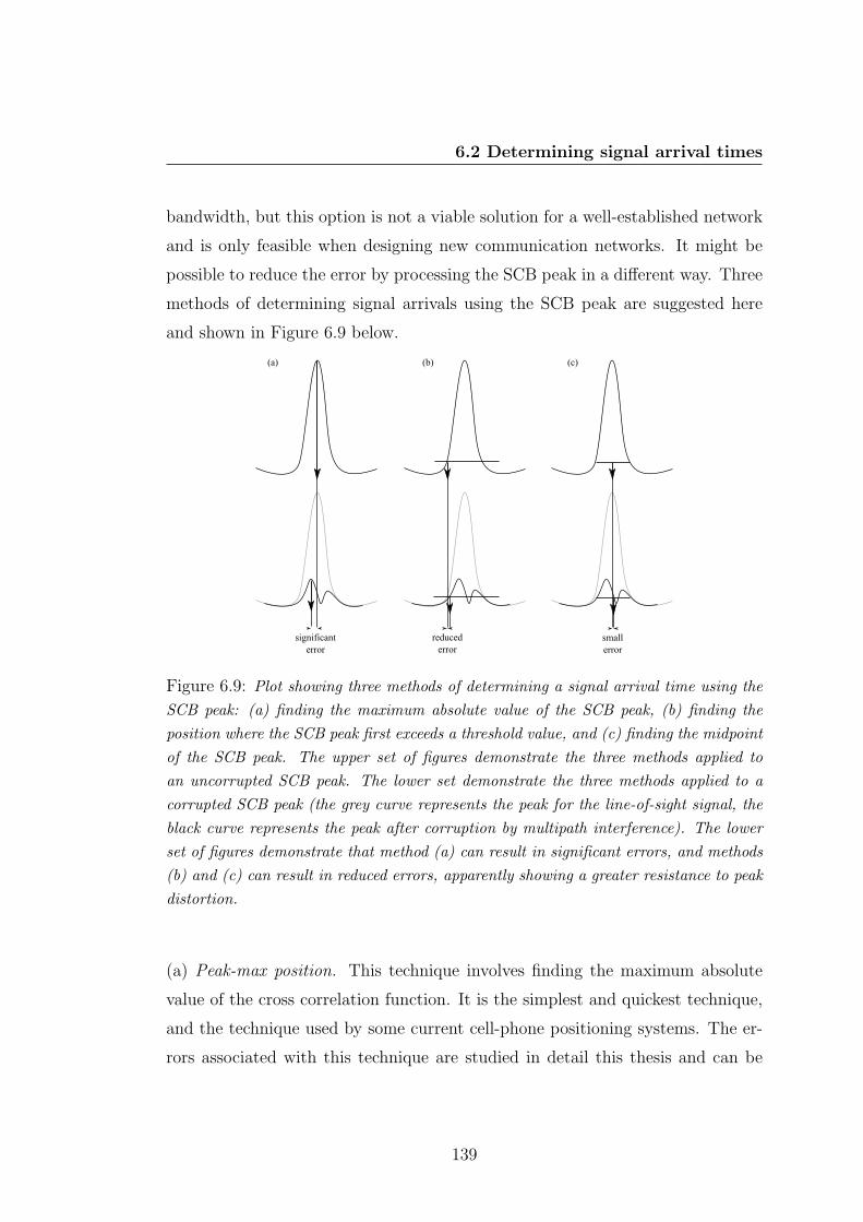
6.2 Determining signal arrival times
bandwidth, but this option is not a viable solution for a well-established network
and is only feasible when designing new communication networks. It might be
possible to reduce the error by processing the SCB peak in a different way. Three
methods of determining signal arrivals using the SCB peak are suggested here
and shown in Figure 6.9 below.
Figure 6.9: Plot showing three methods of determining a signal arrival time using theSCB peak: (a) finding the maximum absolute value of the SCB peak, (b) finding theposition where the SCB peak first exceeds a threshold value, and (c) finding the midpointof the SCB peak. The upper set of figures demonstrate the three methods applied toan uncorrupted SCB peak. The lower set demonstrate the three methods applied to acorrupted SCB peak (the grey curve represents the peak for the line-of-sight signal, theblack curve represents the peak after corruption by multipath interference). The lowerset of figures demonstrate that method (a) can result in significant errors, and methods(b) and (c) can result in reduced errors, apparently showing a greater resistance to peakdistortion.
(a) Peak-max position. This technique involves finding the maximum absolute
value of the cross correlation function. It is the simplest and quickest technique,
and the technique used by some current cell-phone positioning systems. The er-
rors associated with this technique are studied in detail this thesis and can be
139
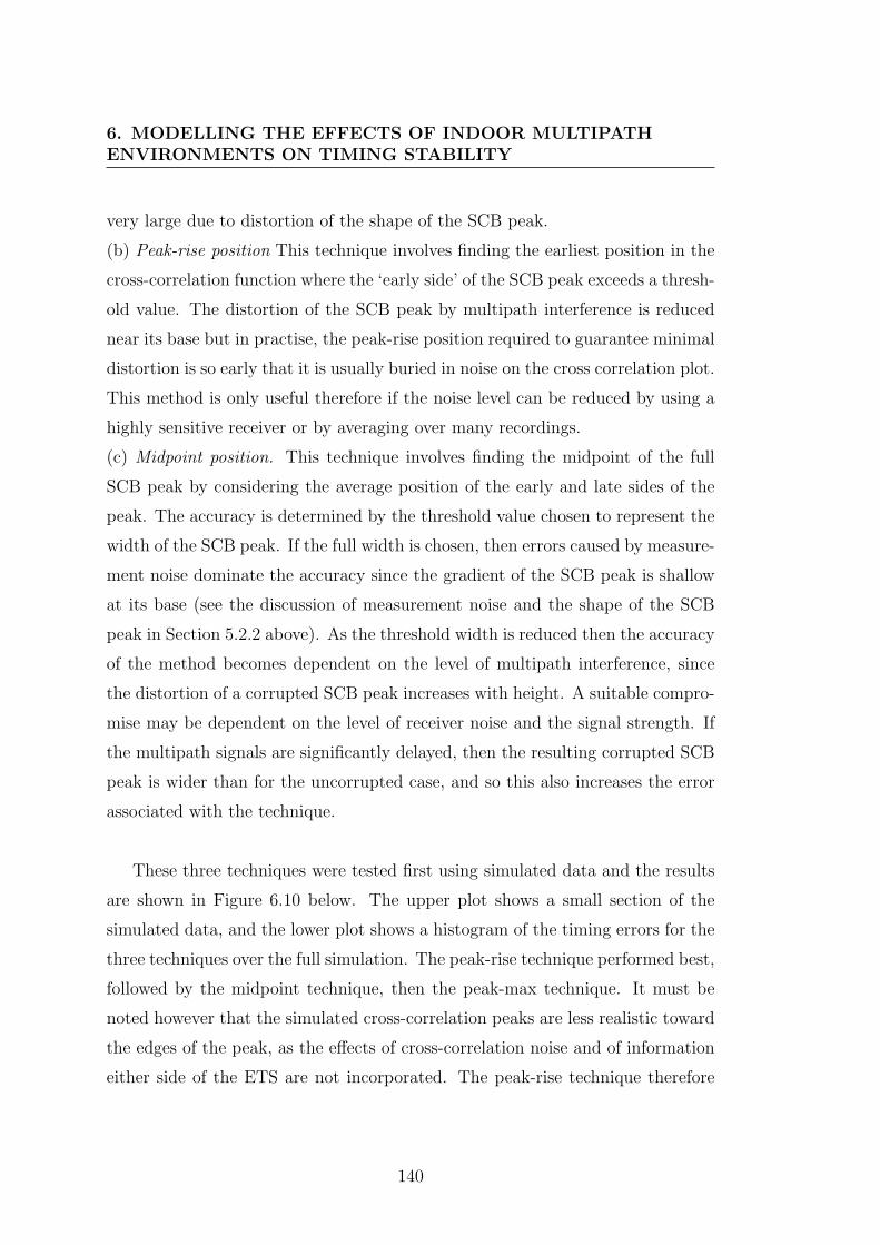
6. MODELLING THE EFFECTS OF INDOOR MULTIPATHENVIRONMENTS ON TIMING STABILITY
very large due to distortion of the shape of the SCB peak.
(b) Peak-rise position This technique involves finding the earliest position in the
cross-correlation function where the ‘early side’ of the SCB peak exceeds a thresh-
old value. The distortion of the SCB peak by multipath interference is reduced
near its base but in practise, the peak-rise position required to guarantee minimal
distortion is so early that it is usually buried in noise on the cross correlation plot.
This method is only useful therefore if the noise level can be reduced by using a
highly sensitive receiver or by averaging over many recordings.
(c) Midpoint position. This technique involves finding the midpoint of the full
SCB peak by considering the average position of the early and late sides of the
peak. The accuracy is determined by the threshold value chosen to represent the
width of the SCB peak. If the full width is chosen, then errors caused by measure-
ment noise dominate the accuracy since the gradient of the SCB peak is shallow
at its base (see the discussion of measurement noise and the shape of the SCB
peak in Section 5.2.2 above). As the threshold width is reduced then the accuracy
of the method becomes dependent on the level of multipath interference, since
the distortion of a corrupted SCB peak increases with height. A suitable compro-
mise may be dependent on the level of receiver noise and the signal strength. If
the multipath signals are significantly delayed, then the resulting corrupted SCB
peak is wider than for the uncorrupted case, and so this also increases the error
associated with the technique.
These three techniques were tested first using simulated data and the results
are shown in Figure 6.10 below. The upper plot shows a small section of the
simulated data, and the lower plot shows a histogram of the timing errors for the
three techniques over the full simulation. The peak-rise technique performed best,
followed by the midpoint technique, then the peak-max technique. It must be
noted however that the simulated cross-correlation peaks are less realistic toward
the edges of the peak, as the effects of cross-correlation noise and of information
either side of the ETS are not incorporated. The peak-rise technique therefore
140
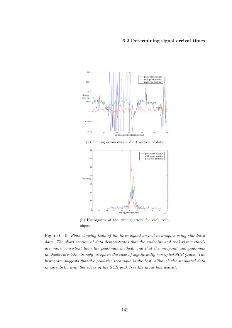
6.2 Determining signal arrival times
0 10 20 30 40 50 60−1E−6
−0.5E−6
0
0.5E−6
1E−6
1.5E−6
2E−6
antenna position (centimetres)
timingerror (s)
peak−max positionmid−point positionpeak−rise position
(a) Timing errors over a short section of data
−5 −4 −3 −2 −1 0 1 2 3 4 5
x 10−6
0
10
20
30
40
50
60
70
timing error (seconds)
frequency
peak−max positionmid−point positionpeak−rise position
(b) Histograms of the timing errors for each tech-nique.
Figure 6.10: Plots showing tests of the three signal-arrival techniques using simulateddata. The short section of data demonstrates that the midpoint and peak-rise methodsare more consistent than the peak-max method, and that the midpoint and peak-maxmethods correlate strongly except in the case of significantly corrupted SCB peaks. Thehistogram suggests that the peak-rise technique is the best, although the simulated datais unrealistic near the edges of the SCB peak (see the main text above).
141
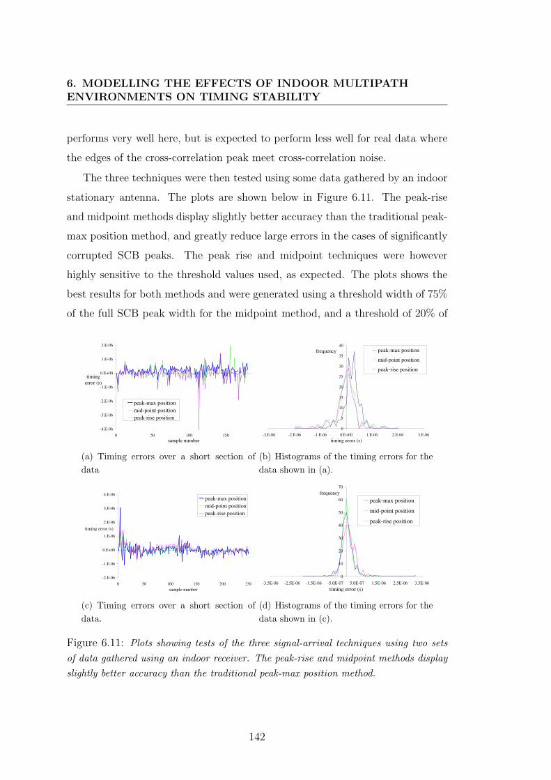
6. MODELLING THE EFFECTS OF INDOOR MULTIPATHENVIRONMENTS ON TIMING STABILITY
performs very well here, but is expected to perform less well for real data where
the edges of the cross-correlation peak meet cross-correlation noise.
The three techniques were then tested using some data gathered by an indoor
stationary antenna. The plots are shown below in Figure 6.11. The peak-rise
and midpoint methods display slightly better accuracy than the traditional peak-
max position method, and greatly reduce large errors in the cases of significantly
corrupted SCB peaks. The peak rise and midpoint techniques were however
highly sensitive to the threshold values used, as expected. The plots shows the
best results for both methods and were generated using a threshold width of 75%
of the full SCB peak width for the midpoint method, and a threshold of 20% of
(a) Timing errors over a short section ofdata
(b) Histograms of the timing errors for thedata shown in (a).
(c) Timing errors over a short section ofdata.
(d) Histograms of the timing errors for thedata shown in (c).
Figure 6.11: Plots showing tests of the three signal-arrival techniques using two setsof data gathered using an indoor receiver. The peak-rise and midpoint methods displayslightly better accuracy than the traditional peak-max position method.
142
6.2 Determining signal arrival times
the full peak height for the peak-rise method.
As a final test with real data, the three techniques were compared using the
data from the initial experiment on the roof (see Figures 5.4 and 5.5) and the
results are given in Figure 6.12 below. In this case, the ability of the peak-
rise and midpoint techniques to reduce large timing errors is clear. The peak-
rise method shows some improvement over the normal peak-max method, but
the midpoint method can be used to reduce large errors caused by corrupted
SCB peaks significantly. However, both the peak-rise and midpoint methods
require more processing power than the peak-position method. A GSM cell phone
samples the incoming signal at 270.833kHz, and so records a sample every 3.7
Figure 6.12: Plot showing tests of the three signal-arrival techniques using the datafrom the initial roof experiment. The peak method results in a large timing error whenthe SCB peaks are significantly corrupted (see Figure 5.5). The peak-rise techniquereduces this error slightly, and the mid-rise technique can be used to minimise theerror.
143
6. MODELLING THE EFFECTS OF INDOOR MULTIPATHENVIRONMENTS ON TIMING STABILITY
microseconds. The SCB peak is about 14 microseconds wide, and so is only
sampled 3 times by a cell phone. In this project, by comparison, the SCB peaks
were sampled 28 or 29 times and then this resolution was increased by a factor of
20 using interpolation. In a cell phone, a simple computation can be performed
to estimate the maximum value of the SCB peak using 3 values, whereas the
improved accuracy of the peak-rise and mid-position techniques are dependent
on either a much higher sampling rate or a processor-intensive interpolation. As
modern cell phones become more sophisticated it is possible that the interpolation
process, and therefore the midpoint technique, may become a feasible solution to
the problem of large timing errors.
The effect of SCB peak corruption on timing errors can also be reduced by in-
creasing the bandwidth of the signal, such that the SCB peak narrows. The third-
generation cell phone networks broadcast signals with 5MHz of bandwidth. The
coherence time of these signals is 0.2 microseconds, and so the cross-correlation
peak of a timing marker is about 0.4 microseconds wide. The timing errors on
the third-generation networks are therefore expected to be noticeably lower than
those experienced on GSM networks, with the main problem being estimating
the earliest arrival from a number of individually resolved timing markers.
6.3 Conclusions
1. Two models are considered in order to simulate the experiments studied in
Chapter 5, a model based on cross correlating signal waveforms (RSI) and a model
based on superimposing truncated raised-cosine functions in order to represent
the superposition of SCB?ETS cross-correlation peaks (CCPI). The two models
produce identical results but the CCPI model requires much less processing time
than the RSI model.
2. Simulations presented here using the CCPI model suggests that smooth vari-
ations in the SCB peak positions can be accounted for by a sparse multipath
144
6.3 Conclusions
environment consisting of a small number of significant signals with similar am-
plitudes, phase differences determined by their path lengths, and some angular
separation all interfering at the receiver.
3. Simulations presented here using the CCPI model suggests that the rapid and
large variations in timing errors indoors cannot be accounted for by signals with
fixed amplitudes interfering at the receiver. If the amplitudes of the signals vary
randomly at each position, then the behaviour seen in the Electronics Laboratory
can be simulated. Randomly varying the phase or path lengths (within reason-
able limits) alone cannot reproduce this behaviour.
4. The rapid variations in signal amplitude proposed can be accounted for by
movement of people and small changes in receiver position. As the receiver posi-
tion varies, the exact path each signal takes to reach that point changes and so
do the densities and exact structures of walls and objects along those paths. If
the path involves scattering or diffraction then slight changes in receiver position
will also result in different receiver amplitudes due to the exact polar pattern at
the diffracting or scattering object. A given signal path may also be temporarily
attenuated or scattered by the movement of people and objects in the local envi-
ronment.
5. Two methods are proposed to increase the accuracy when determining signal
arrival times, the peak-rise method and the midpoint method. Both methods
demonstrate an improvement in accuracy by reducing, and in some cases remov-
ing, the most extreme errors in a given data set. However, both methods require
more intensive computation than the simple peak-position technique.
145

6. MODELLING THE EFFECTS OF INDOOR MULTIPATHENVIRONMENTS ON TIMING STABILITY
146
Chapter 7
A study of the timing errors
encountered when performing
radio-location using the GSM
network
A series of experiments was performed in order to study the accuracy of position-
ing systems in various environments using the signals radiated by the transmitters
of the GSM network. The distances between a receiver and a reference GSM base
station were measured by considering the synchronisation burst on the base sta-
tion’s control channel (see Section in Chapter 3). These distances were then
compared to those determined using a GPS device or accurate mapping. Ru-
ral, suburban, light urban, mid urban, and indoor environments in and around
Cambridge were surveyed.
Whenever SCB signals are used to calculate a position, it is usually under two
assumptions. The first of these is that an unbiased and consistent measurement
of the signal’s arrival time can be made using a feature of the cross correlation
between the incoming signal and the ETS. The simplest feature is the maximum
absolute value, but there are many other possibilities. This property is used
here because (a) it is the feature currently used Cambridge Positioning Systems’
147
7. A STUDY OF THE TIMING ERRORS ENCOUNTEREDWHEN PERFORMING RADIO-LOCATION USING THE GSMNETWORK
products, and (b) it illustrates very well many of the effects which are common
to the use of all features. The second assumption is that the resulting estimate
of a signal’s time of flight is the same as the line of sight time of flight and so is
representative of the linear distance between the base station and receiver. These
assumptions are tested in this chapter.
7.1 Definitions of environment
A simple set of rules was formulated to determine the general nature of a given
outdoor environment.
Rural: A rural area has well-spaced, one- or two-storey buildings, many trees, and
narrow roads through farmland, fields and small villages. Grantchester village and
its surrounding farm tracks were used for this survey.
Suburban: A suburban area is located on the edges of a city, with one- and
two-storey detached and semi-detached housing. The spacing between buildings
across roads is larger than the height of the buildings. Trees are also a dominant
feature of this environment.
Light-urban: A light-urban environment features two-storey terraced housing and
terraced rows of shops or businesses. The distances between buildings across a
road are often comparable with, or less than, the heights of the buildings.
Mid-urban: A mid-urban area has larger buildings (exceeding two storeys) and
they are typically offices, stores and apartment blocks. The distances between
buildings across roads are less than their heights. Lamp posts and traffic signs
are also a major feature of this environment.
Dense-urban: A dense-urban environment is usually found in the central areas
of large cities and consists of urban canyons with very tall buildings in every
direction, very few trees but an appreciable density of lamp posts and traffic
signs. There was not an area fitting this definition (e.g. central London) close
enough to the Cavendish Laboratory for a feasible survey to take place.
148
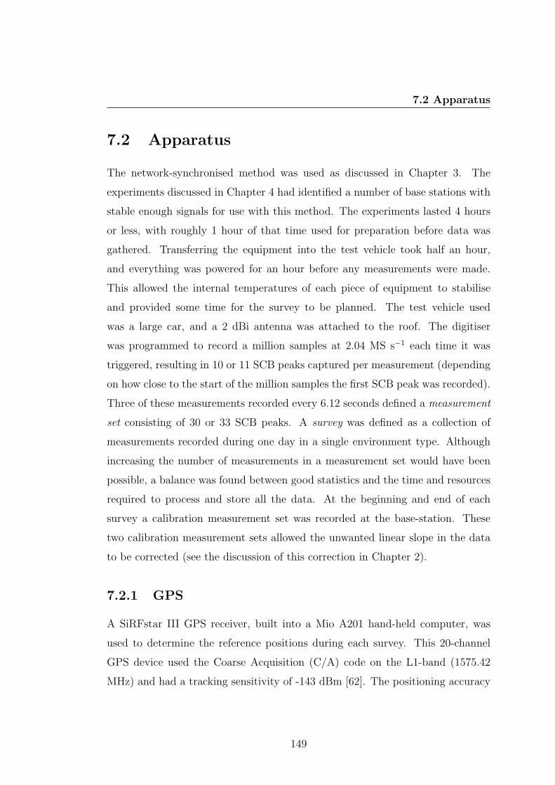
7.2 Apparatus
7.2 Apparatus
The network-synchronised method was used as discussed in Chapter 3. The
experiments discussed in Chapter 4 had identified a number of base stations with
stable enough signals for use with this method. The experiments lasted 4 hours
or less, with roughly 1 hour of that time used for preparation before data was
gathered. Transferring the equipment into the test vehicle took half an hour,
and everything was powered for an hour before any measurements were made.
This allowed the internal temperatures of each piece of equipment to stabilise
and provided some time for the survey to be planned. The test vehicle used
was a large car, and a 2 dBi antenna was attached to the roof. The digitiser
was programmed to record a million samples at 2.04 MS s−1 each time it was
triggered, resulting in 10 or 11 SCB peaks captured per measurement (depending
on how close to the start of the million samples the first SCB peak was recorded).
Three of these measurements recorded every 6.12 seconds defined a measurement
set consisting of 30 or 33 SCB peaks. A survey was defined as a collection of
measurements recorded during one day in a single environment type. Although
increasing the number of measurements in a measurement set would have been
possible, a balance was found between good statistics and the time and resources
required to process and store all the data. At the beginning and end of each
survey a calibration measurement set was recorded at the base-station. These
two calibration measurement sets allowed the unwanted linear slope in the data
to be corrected (see the discussion of this correction in Chapter 2).
7.2.1 GPS
A SiRFstar III GPS receiver, built into a Mio A201 hand-held computer, was
used to determine the reference positions during each survey. This 20-channel
GPS device used the Coarse Acquisition (C/A) code on the L1-band (1575.42
MHz) and had a tracking sensitivity of -143 dBm [62]. The positioning accuracy
149
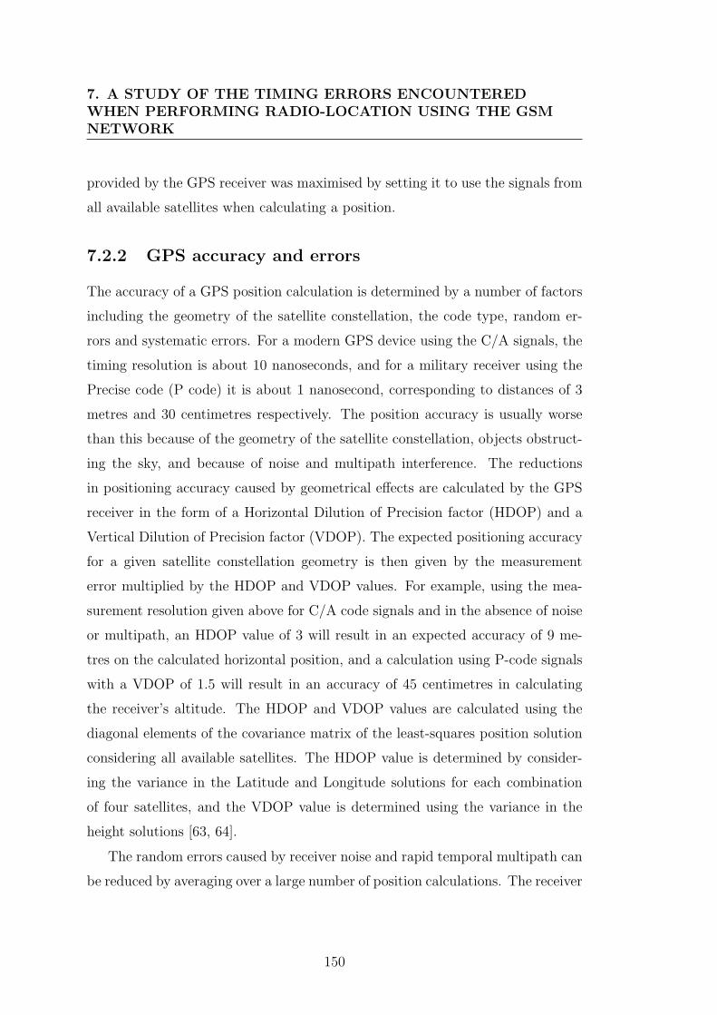
7. A STUDY OF THE TIMING ERRORS ENCOUNTEREDWHEN PERFORMING RADIO-LOCATION USING THE GSMNETWORK
provided by the GPS receiver was maximised by setting it to use the signals from
all available satellites when calculating a position.
7.2.2 GPS accuracy and errors
The accuracy of a GPS position calculation is determined by a number of factors
including the geometry of the satellite constellation, the code type, random er-
rors and systematic errors. For a modern GPS device using the C/A signals, the
timing resolution is about 10 nanoseconds, and for a military receiver using the
Precise code (P code) it is about 1 nanosecond, corresponding to distances of 3
metres and 30 centimetres respectively. The position accuracy is usually worse
than this because of the geometry of the satellite constellation, objects obstruct-
ing the sky, and because of noise and multipath interference. The reductions
in positioning accuracy caused by geometrical effects are calculated by the GPS
receiver in the form of a Horizontal Dilution of Precision factor (HDOP) and a
Vertical Dilution of Precision factor (VDOP). The expected positioning accuracy
for a given satellite constellation geometry is then given by the measurement
error multiplied by the HDOP and VDOP values. For example, using the mea-
surement resolution given above for C/A code signals and in the absence of noise
or multipath, an HDOP value of 3 will result in an expected accuracy of 9 me-
tres on the calculated horizontal position, and a calculation using P-code signals
with a VDOP of 1.5 will result in an accuracy of 45 centimetres in calculating
the receiver’s altitude. The HDOP and VDOP values are calculated using the
diagonal elements of the covariance matrix of the least-squares position solution
considering all available satellites. The HDOP value is determined by consider-
ing the variance in the Latitude and Longitude solutions for each combination
of four satellites, and the VDOP value is determined using the variance in the
height solutions [63, 64].
The random errors caused by receiver noise and rapid temporal multipath can
be reduced by averaging over a large number of position calculations. The receiver
150
7.2 Apparatus
Figure 7.1: This figure shows the effects of good and bad satellite geometry on theaccuracy of a GPS position. The sketch is shown in two dimensions, but the principleis easily extended to three. The curved pink lines represent the possible position of areceiver that has measured a certain arrival time from a given satellite. The thicknessof the lines represents the error on the measurement. The sketch on the left representsa good satellite geometry, with three satellites evenly distributed and well spread outacross the measurement plane. The black area highlighting the region intersected by allthree signals represents the region of uncertainty in the receiver position. The figure onthe right represents a poor signal geometry, with all three sources lying roughly along aline. The intersecting region is much larger for this geometry, leading to a reduction inthe positioning accuracy.
noise and multipath constitute, in effect, “dither noise” and usually dominate over
the timing resolution of the receiver. In these circumstances, the average position
of a stationary receiver can result in a higher positioning accuracy. However,
static multipath interference represents a systematic error at a stationary receiver
and its effect cannot be reduced by averaging.
The systematic errors as a result of daily changes in the atmospheric conditions
such as tropospheric effects (±0.7 metres), ionospheric effects (±4 metres), errors
in ephemeris data (±2 metres) and drifts in the satellite clocks (±3 metres) cannot
just be averaged out of the system. However, since the errors are systematic,
the relative distances between a set of points will still be determined to a high
151
7. A STUDY OF THE TIMING ERRORS ENCOUNTEREDWHEN PERFORMING RADIO-LOCATION USING THE GSMNETWORK
accuracy by a static GPS receiver although their absolute positions may all be
systematically displaced from their true value. The surveys performed here used
relative measurements (a calibration GPS reading was taken at the BTS at the
start and end of the experiment), and so in principle the GPS error was expected
to be dominated by the random errors and therefore reduced by averaging (each
GPS position recorded in the surveys was actually an average of 50 values).
However, since each survey took a number of hours to complete, the factors which
affected the systematic errors may have varied in that time. In order to account
for this possibility the difference between calibration measurements recorded three
hours apart was considered. An averaged GPS position was recorded in a fixed
location on the roof of the Cavendish Laboratory twice a day for 12 days. The
experiment was performed at 2 pm and 5 pm each day since these were typically
the times of the calibration measurement sets during the surveys. The satellite
availability and geometry were always good from the laboratory roof, with at
least 8 satellites available and an HDOP of 1–1.2 for each data point. This was
also a feature of the real calibration experiments as the base stations were in open
areas. The data had a standard deviation of 4 metres as shown below in Figure
7.2. This standard deviation was used as the error on each GPS position in the
surveying experiments.
The horizontal distances from the BTS (according to GPS measurements) and
the measured GSM signal flight times are being compared in these experiments,
so the error associated with VDOP was not considered. The horizontal distance
according to the GSM flight time was determined by using Pythagoras’ theorem
and the knowledge of the heights of a given BTS and the GSM receiver (see
Figure 7.3 below).
7.3 Method
The method used to gather data was similar to that used for the experiments
described in Chapter 4, with the digitiser being triggered continuously every 6.12
152
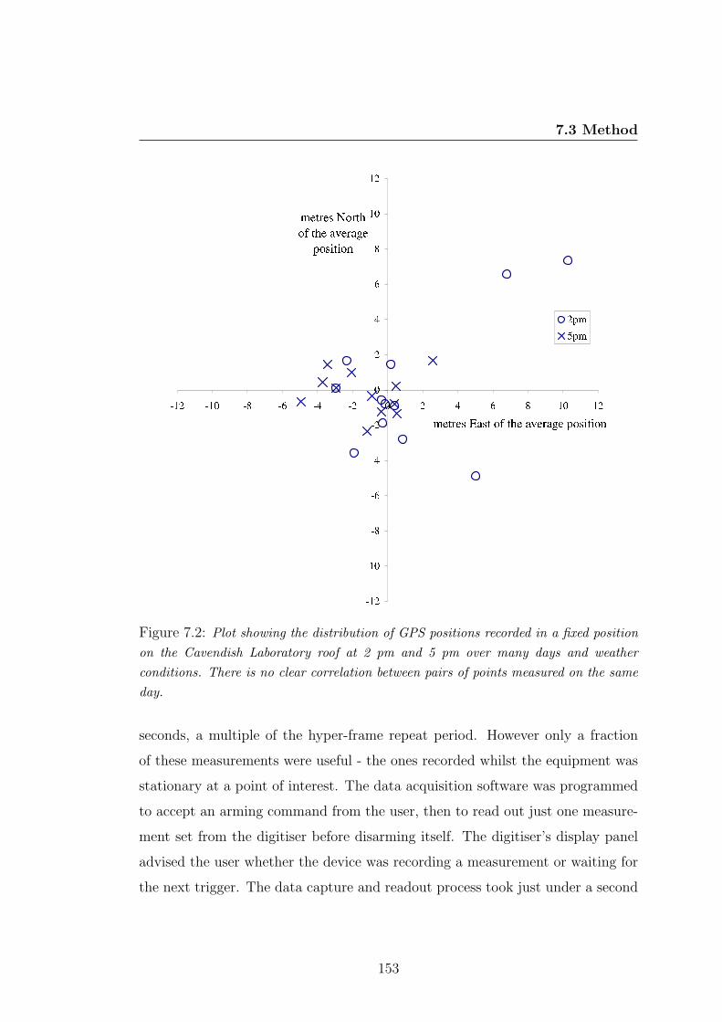
7.3 Method
Figure 7.2: Plot showing the distribution of GPS positions recorded in a fixed positionon the Cavendish Laboratory roof at 2 pm and 5 pm over many days and weatherconditions. There is no clear correlation between pairs of points measured on the sameday.
seconds, a multiple of the hyper-frame repeat period. However only a fraction
of these measurements were useful - the ones recorded whilst the equipment was
stationary at a point of interest. The data acquisition software was programmed
to accept an arming command from the user, then to read out just one measure-
ment set from the digitiser before disarming itself. The digitiser’s display panel
advised the user whether the device was recording a measurement or waiting for
the next trigger. The data capture and readout process took just under a second
153
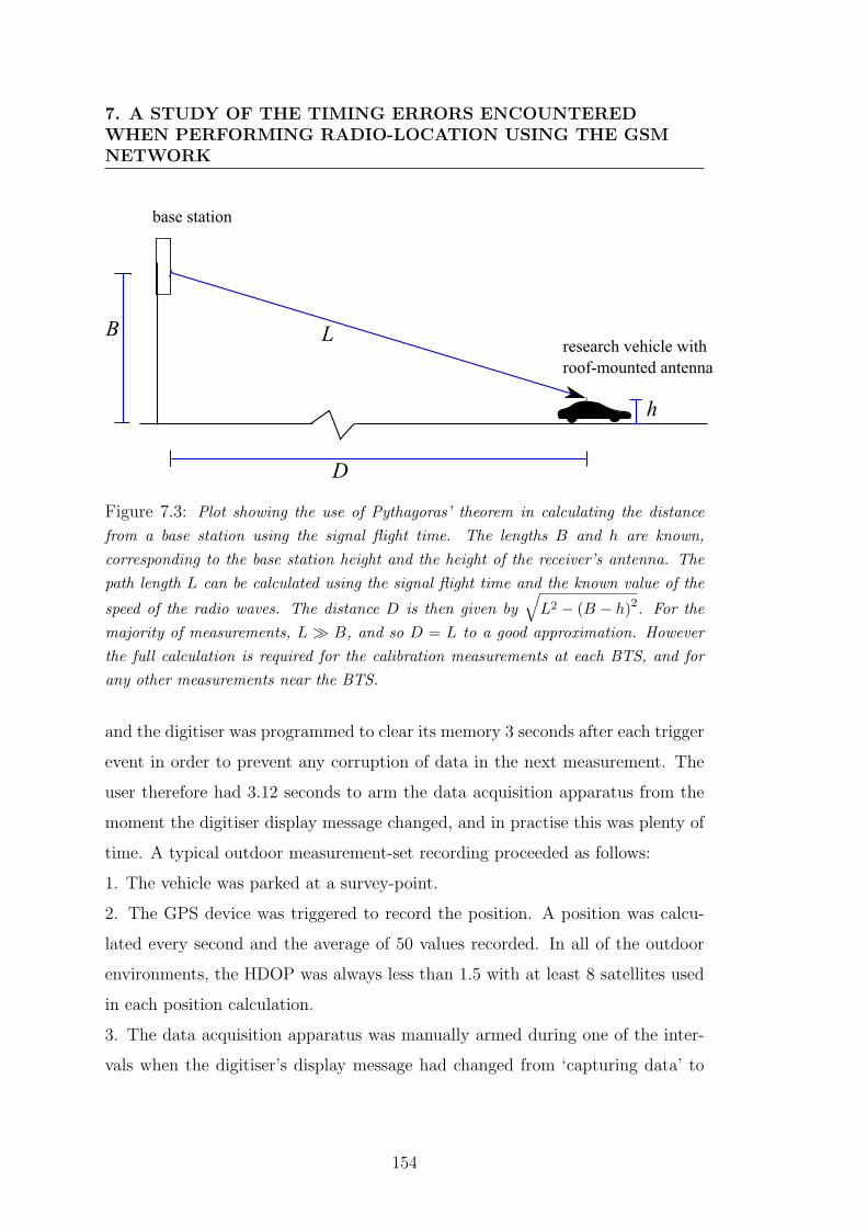
7. A STUDY OF THE TIMING ERRORS ENCOUNTEREDWHEN PERFORMING RADIO-LOCATION USING THE GSMNETWORK
Figure 7.3: Plot showing the use of Pythagoras’ theorem in calculating the distancefrom a base station using the signal flight time. The lengths B and h are known,corresponding to the base station height and the height of the receiver’s antenna. Thepath length L can be calculated using the signal flight time and the known value of the
speed of the radio waves. The distance D is then given by√
L2 − (B − h)2. For themajority of measurements, L B, and so D = L to a good approximation. Howeverthe full calculation is required for the calibration measurements at each BTS, and forany other measurements near the BTS.
and the digitiser was programmed to clear its memory 3 seconds after each trigger
event in order to prevent any corruption of data in the next measurement. The
user therefore had 3.12 seconds to arm the data acquisition apparatus from the
moment the digitiser display message changed, and in practise this was plenty of
time. A typical outdoor measurement-set recording proceeded as follows:
1. The vehicle was parked at a survey-point.
2. The GPS device was triggered to record the position. A position was calcu-
lated every second and the average of 50 values recorded. In all of the outdoor
environments, the HDOP was always less than 1.5 with at least 8 satellites used
in each position calculation.
3. The data acquisition apparatus was manually armed during one of the inter-
vals when the digitiser’s display message had changed from ‘capturing data’ to
154
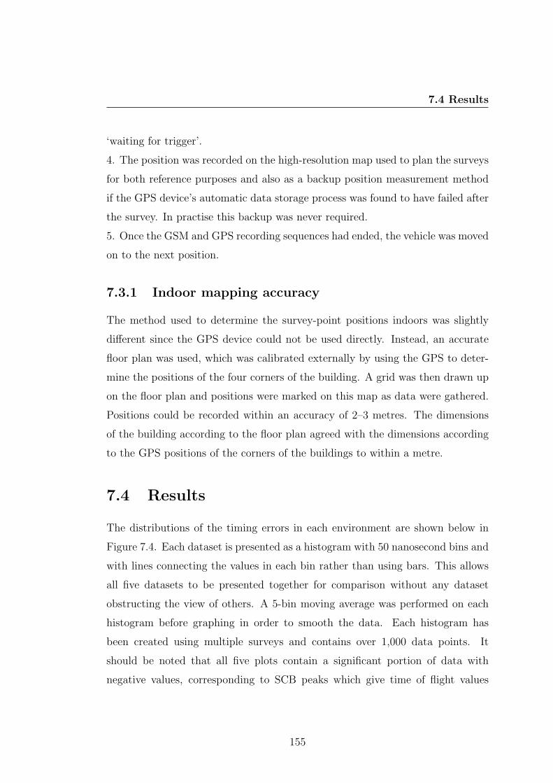
7.4 Results
‘waiting for trigger’.
4. The position was recorded on the high-resolution map used to plan the surveys
for both reference purposes and also as a backup position measurement method
if the GPS device’s automatic data storage process was found to have failed after
the survey. In practise this backup was never required.
5. Once the GSM and GPS recording sequences had ended, the vehicle was moved
on to the next position.
7.3.1 Indoor mapping accuracy
The method used to determine the survey-point positions indoors was slightly
different since the GPS device could not be used directly. Instead, an accurate
floor plan was used, which was calibrated externally by using the GPS to deter-
mine the positions of the four corners of the building. A grid was then drawn up
on the floor plan and positions were marked on this map as data were gathered.
Positions could be recorded within an accuracy of 2–3 metres. The dimensions
of the building according to the floor plan agreed with the dimensions according
to the GPS positions of the corners of the buildings to within a metre.
7.4 Results
The distributions of the timing errors in each environment are shown below in
Figure 7.4. Each dataset is presented as a histogram with 50 nanosecond bins and
with lines connecting the values in each bin rather than using bars. This allows
all five datasets to be presented together for comparison without any dataset
obstructing the view of others. A 5-bin moving average was performed on each
histogram before graphing in order to smooth the data. Each histogram has
been created using multiple surveys and contains over 1,000 data points. It
should be noted that all five plots contain a significant portion of data with
negative values, corresponding to SCB peaks which give time of flight values
155
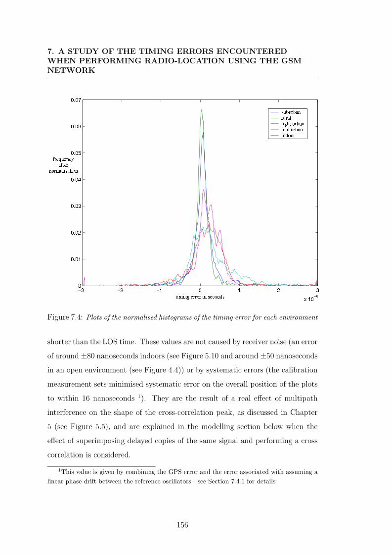
7. A STUDY OF THE TIMING ERRORS ENCOUNTEREDWHEN PERFORMING RADIO-LOCATION USING THE GSMNETWORK
Figure 7.4: Plots of the normalised histograms of the timing error for each environment
shorter than the LOS time. These values are not caused by receiver noise (an error
of around ±80 nanoseconds indoors (see Figure 5.10 and around ±50 nanoseconds
in an open environment (see Figure 4.4)) or by systematic errors (the calibration
measurement sets minimised systematic error on the overall position of the plots
to within 16 nanoseconds 1). They are the result of a real effect of multipath
interference on the shape of the cross-correlation peak, as discussed in Chapter
5 (see Figure 5.5), and are explained in the modelling section below when the
effect of superimposing delayed copies of the same signal and performing a cross
correlation is considered.
1This value is given by combining the GPS error and the error associated with assuming alinear phase drift between the reference oscillators - see Section 7.4.1 for details
156
7.4 Results
The histograms show that the timing error distributions for rural and subur-
ban environments were narrower than for the urban and indoor environments as
expected. The majority of the rural and suburban values (66%) lie in the range
-0.33 to 0.33 microseconds, corresponding to errors of ±100 metres. The urban
and indoor environments have a similar proportion of values within the range
-0.5 to 0.8 microseconds, corresponding to errors in the range of -150 metres to
240 metres. All of the environment types contain a small number of values with
errors of ±600 metres or more. The urban and indoor distributions are also not
symmetrical about zero, but contain more positive timing error values than neg-
ative. This suggests that there is either a mean, non-zero signal delay in these
environment types, or that moderate and dense multipath interference results
in a bias towards positive timing errors. The modelling performed in Chapter
6 suggests that the latter may be true (see the peak-max position histograms
in Figures 6.10 and 6.11), but in either case, the result is an effective mean or
‘typical’ signal delay value in these environments.
The indoor data set also exhibits three distinct and equally spaced peaks,
which may have been caused by resonance with the particular dimensions and
layout of the building’s interior. The building used for the indoor tests (The
Rutherford building of the Cavendish Laboratory) contained a number of small
rooms connected by long corridors. The short corridors were approximately 26
metres long, and the long corridors were approximately 63 metres long. The spac-
ing between the first two peaks in the data corresponds to a difference of about 50
metres and the spacing between the first and last peaks in the data correspond to
a difference of about 120 metres. These extra peaks may have been caused by the
strongest received signal propagating along the corridors before scattering to a
receiver, or alternatively by signals entering the building from different directions
after reflecting or scattering from other nearby buildings. Figure 7.5 below shows
a sketch of the floor plan of the building used for the survey. The ground floor
and first floor were both included in the survey, and the layout of both floors
is identical apart from a glass walkway connecting the first floor of the building
157
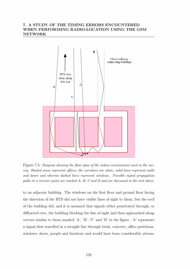
7. A STUDY OF THE TIMING ERRORS ENCOUNTEREDWHEN PERFORMING RADIO-LOCATION USING THE GSMNETWORK
Figure 7.5: Diagram showing the floor plan of the indoor environment used in the sur-vey. Shaded areas represent offices, the corridors are white, solid lines represent wallsand doors and whereas dashed lines represent windows. Possible signal propagationpaths to a receiver point are marked A, B, C and D and are discussed in the text above.
to an adjacent building. The windows on the first floor and ground floor facing
the direction of the BTS did not have visible lines of sight to them, but the roof
of the building did, and it is assumed that signals either penetrated through, or
diffracted over, the building blocking the line of sight and then approached along
vectors similar to those marked ‘A’, ‘B’, ‘C’ and ‘D’ in the figure. ‘A’ represents
a signal that travelled in a straight line through brick, concrete, office partitions,
windows, doors, people and furniture and would have been considerably attenu-
158
7.4 Results
ated. ‘B’ represents a signal that entered the glass walkway and propagated down
the corridor before diffracting or reflecting toward reception points. ‘C’ shows a
possible mechanism which could have increased the delay of a given signal con-
siderably by including reflections from metal filing cabinets and cupboards in the
corridors in order to allow a signal to reverberate in a corridor before reaching
a reception point. ‘D’ shows another possible mechanism involving propagation
along the corridors. It is also possible that signals reflected from the buildings
beyond the Cavendish Laboratory (not shown in the diagram, but off the bottom
of the sketch) and entered the surveyed building from the far side, propagating
back toward the BTS. These signals would have then had an extra path length of
roughly 150 metres. However, there was no clear correlation between these dis-
tinct peaks and any general areas within the building, suggesting that the indoor
signal environment is complex and varies on a fine spatial scale.
7.4.1 Error analysis
The error in the determination of an individual SCB peak position was affected by
a number of factors including the stabilities of the frequency standards used by the
measuring equipment and the BTS, errors in the reference positions determined
by GPS or accurate mapping, and the error introduced by up-sampling noisy
data.
The stability of the RFS was measured in an experiment discussed in Chapter
2 which showed that the average error associated with the assumption of a linear
phase drift between two identical RFS oscillators over a 3 hour test was about
9 nanoseconds. It was also shown in Chapter 4 that the long-term stabilities
of certain local base stations on Network 1 were similar to that of the FRK-
H Rubidium oscillator, and those particular base stations were the only ones
used in the experiments described in this chapter. The results from Chapter 2
therefore provide an approximation to the error associated with the linear-phase-
drift corrections for these experiments. The full value of this error only applied to
159
7. A STUDY OF THE TIMING ERRORS ENCOUNTEREDWHEN PERFORMING RADIO-LOCATION USING THE GSMNETWORK
measurements performed toward the end of a three hour test, with measurements
closer to the beginning of the test having a proportionately lower error.
The timing error due to measurement noise for a stationary indoor receiver
was shown in Figure 5.10 to be about ±80 nanoseconds, and the measurement
noise at an outdoor receiver was shown to be about ±50 nanoseconds (see Figure
4.4),
The error associated with GPS positioning was shown in the discussion above
to be 4 metres, corresponding to a 13 nanoseconds timing error on each GPS
measurement. Although averaging improved the GPS accuracy, the work above
demonstrated that there was an upper bound of approximately 4 metres on the er-
ror when performing relative measurements over the course of about three hours.
The resolution of an SCB peak position after up-sampling was 24.5 nanosec-
onds, giving a measurement resolution error of 12.25 nanoseconds.
Combining all of these independent errors in quadrature (and noting that two
GPS and two SCB-peak measurements are used per time of flight calculation)
gave a total maximum error on an indoor measurement 3 hours after a cali-
bration measurement of 97 nanoseconds. With the error caused by drift in the
frequency standards discounted, the total error is 96 nanoseconds. For a short
outdoor test (such that the GPS errors can be ignored) this error drops to 73
nanoseconds. These errors were larger than the bin size used to produce the
histograms (50 nanoseconds) but the 5-bin moving average used to smooth the
data also reduced the error caused by any data points in the wrong bin. The
measurement noise clearly dominates the error in these recordings, and can be
reduced by averaging over many recordings. However, in producing these timing
error distributions, each recording was considered separately so that the effects
of rapid temporal multipath variations (which contribute randomly to the overall
error on a measurement) could be recorded and studied rather than averaged out.
160
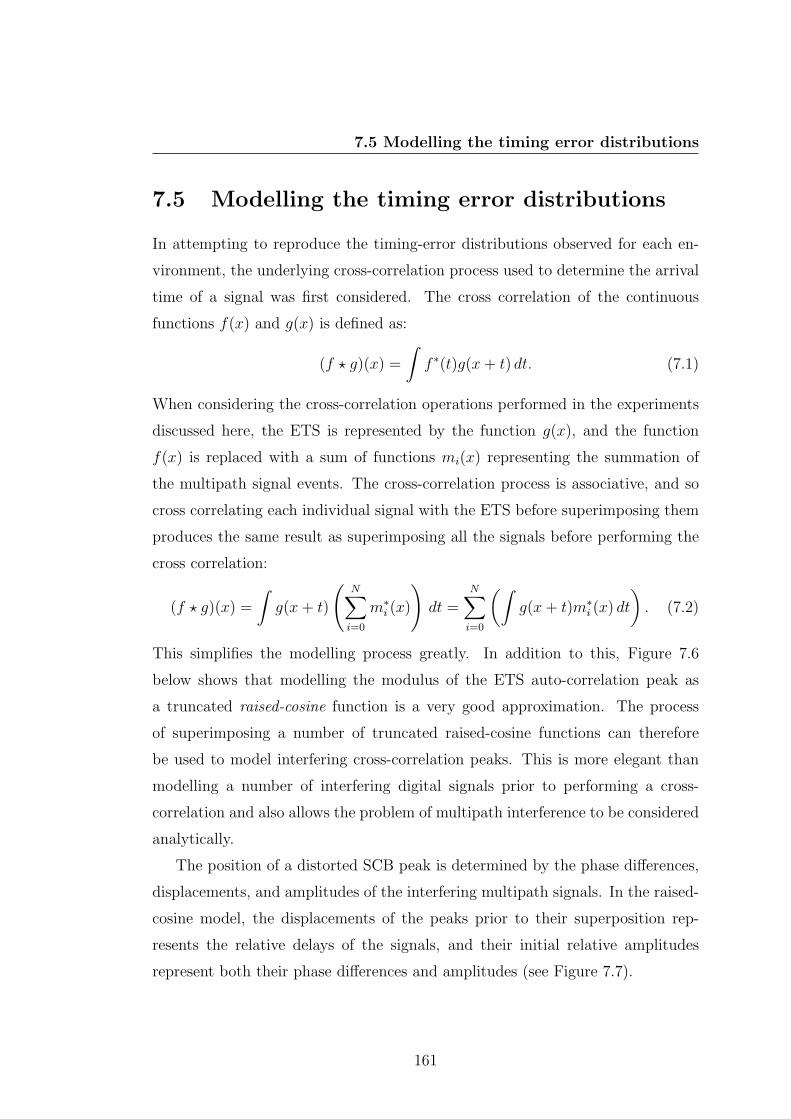
7.5 Modelling the timing error distributions
7.5 Modelling the timing error distributions
In attempting to reproduce the timing-error distributions observed for each en-
vironment, the underlying cross-correlation process used to determine the arrival
time of a signal was first considered. The cross correlation of the continuous
functions f(x) and g(x) is defined as:
(f ? g)(x) =
∫f ∗(t)g(x+ t) dt. (7.1)
When considering the cross-correlation operations performed in the experiments
discussed here, the ETS is represented by the function g(x), and the function
f(x) is replaced with a sum of functions mi(x) representing the summation of
the multipath signal events. The cross-correlation process is associative, and so
cross correlating each individual signal with the ETS before superimposing them
produces the same result as superimposing all the signals before performing the
cross correlation:
(f ? g)(x) =
∫g(x+ t)
(N∑i=0
m∗i (x)
)dt =
N∑i=0
(∫g(x+ t)m∗
i (x) dt
). (7.2)
This simplifies the modelling process greatly. In addition to this, Figure 7.6
below shows that modelling the modulus of the ETS auto-correlation peak as
a truncated raised-cosine function is a very good approximation. The process
of superimposing a number of truncated raised-cosine functions can therefore
be used to model interfering cross-correlation peaks. This is more elegant than
modelling a number of interfering digital signals prior to performing a cross-
correlation and also allows the problem of multipath interference to be considered
analytically.
The position of a distorted SCB peak is determined by the phase differences,
displacements, and amplitudes of the interfering multipath signals. In the raised-
cosine model, the displacements of the peaks prior to their superposition rep-
resents the relative delays of the signals, and their initial relative amplitudes
represent both their phase differences and amplitudes (see Figure 7.7).
161
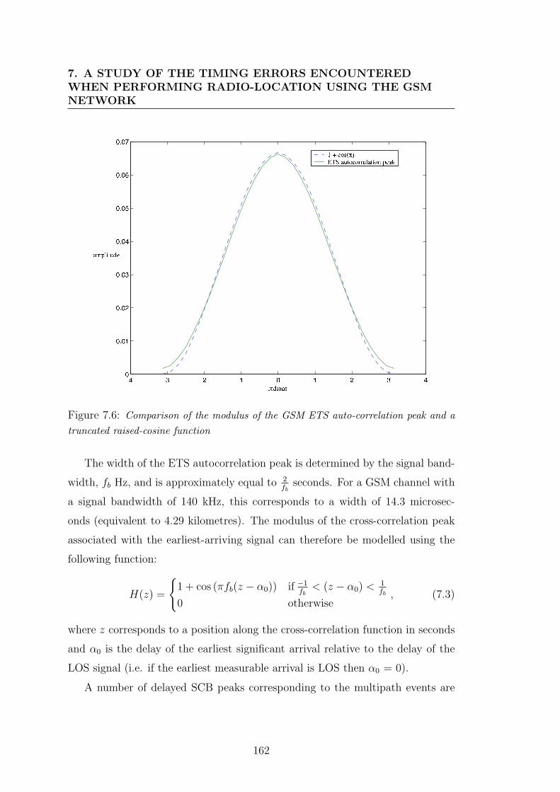
7. A STUDY OF THE TIMING ERRORS ENCOUNTEREDWHEN PERFORMING RADIO-LOCATION USING THE GSMNETWORK
Figure 7.6: Comparison of the modulus of the GSM ETS auto-correlation peak and atruncated raised-cosine function
The width of the ETS autocorrelation peak is determined by the signal band-
width, fb Hz, and is approximately equal to 2fb
seconds. For a GSM channel with
a signal bandwidth of 140 kHz, this corresponds to a width of 14.3 microsec-
onds (equivalent to 4.29 kilometres). The modulus of the cross-correlation peak
associated with the earliest-arriving signal can therefore be modelled using the
following function:
H(z) =
1 + cos (πfb(z − α0)) if −1
fb< (z − α0) <
1fb
0 otherwise, (7.3)
where z corresponds to a position along the cross-correlation function in seconds
and α0 is the delay of the earliest significant arrival relative to the delay of the
LOS signal (i.e. if the earliest measurable arrival is LOS then α0 = 0).
A number of delayed SCB peaks corresponding to the multipath events are
162
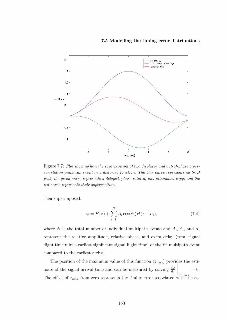
7.5 Modelling the timing error distributions
Figure 7.7: Plot showing how the superposition of two displaced and out-of-phase cross-correlation peaks can result in a distorted function. The blue curve represents an SCBpeak; the green curve represents a delayed, phase rotated, and attenuated copy; and thered curve represents their superposition.
then superimposed:
ψ = H(z) +N∑i=1
Ai cos(φi)H(z − αi), (7.4)
where N is the total number of individual multipath events and Ai, φi, and αi
represent the relative amplitude, relative phase, and extra delay (total signal
flight time minus earliest significant signal flight time) of the ith multipath event
compared to the earliest arrival.
The position of the maximum value of this function (zmax) provides the esti-
mate of the signal arrival time and can be measured by solving dψdz
∣∣∣∣z=zmax
= 0.
The offset of zmax from zero represents the timing error associated with the as-
163
7. A STUDY OF THE TIMING ERRORS ENCOUNTEREDWHEN PERFORMING RADIO-LOCATION USING THE GSMNETWORK
sumption that the peak of the function corresponds to the LOS arrival.
dψ
dz
∣∣∣∣z=zmax
=− πfb sin (πfb(zmax − α0))
− πfb
N∑i=1
Ai cos(φi) sin(πfb(zmax − α0 − αi)) = 0. (7.5)
Now using the trigonometric identity
sin(a− b) = sin(a) cos(b)− cos(a) sin(b), (7.6)
and rearranging gives
tan (πfb(zmax − α0)) =
∑Ni=1Ai cos(φi) sin(πfbαi)
1 +∑N
i=1Ai cos(φi) cos(πfbαi). (7.7)
The distributions of two new variables, x and y, can now be considered, corre-
sponding to the results of the two sums in Equation 7.7 above. According to
the central limit theorem [65], and on the assumption that the processes are ran-
domly distributed and uncorrelated, as the value of N increases, the distributions
of x and y tend to Gaussian distributions. This assumption can be verified by
using suitable values for N and suitable distributions for A, φ and α, as shown in
detail in Appendix A. The two probability densities functions (pdfs) for the new
variables are given by
(N∑i=1
Ai cos(φi) sin(πfbαi)
)=
1√2πσy
exp− y2
2σ2y (7.8)
and
(1 +
N∑i=1
Ai cos(φi) cos(πfbαi)
)=
1√2πσx
exp− (x−1)2
2σ2x , (7.9)
and can be used to determine the probability distribution of zmax. The joint pdf
for a function dependant on both of these distributions is given by the bivariate
Gaussian distribution:
pdf(x, y) =1
2πσxσy√
1− p2exp
− ξ
2(1−p2) , (7.10)
164
7.5 Modelling the timing error distributions
where, in this case,
ξ =(x− 1)2
2σ2x
− 2p(x− 1)y
σxσy+y2
σ2y
(7.11)
and p = correlation(x, y) = σx,y
σxσy.
In Equation 7.7, the two distributions are combined as a ratio, and the ratio
distribution described by Fieller [66] is now considered. For the ratio v = yx,
where x and y are distributed according to the joint pdf f(x, y), the pdf of v is
given by:
pdf(v) =
∫ ∞
−∞|x|f(x, vx) dx, (7.12)
which gives
pdf(v) =
∫ ∞
−∞|x|exp
−
(x−1)2
2σ2x
− 2p(x−1)vxσxσy
+(vx)2
σ2y
2(1−p2)
2πσxσy√
1− p2dx. (7.13)
The solution of this integral, given by Fieller, is
pdf(v) =σxσy
√1− p2
π(v2σ2x − 2pvσxσy + σ2
y)× exp
− 1
2σ2x(1−p2)
+σy(vpσx − σy)
π(v2σ2x − 2pvσxσy + σ2
y)32
× exp−v2
2(v2σ2x−2pvσxσy+σ2
y) ×∫ σy(vpσx−σy)
σxσy
√(1−p2)(v2σ2
x−2pvσxσy+σ2y)
0
exp−v2
2 dv. (7.14)
The probability density function of zmax can be determined using this equation
by noting from Equation 7.7 that
tan(πfb(zmax − α0)) = v. (7.15)
If the pdf of an independent random variable τ is given as f(τ), then the pdf of
µ, where µ = g(τ), is given by
pdf(µ) = |(g′(g−1(µ)))−1|f(g−1(µ)). (7.16)
Substitution of the parameters f(τ) = pdf(v) and µ = g(v) = arctan(v) gives
pdf(zmax) = |(1 + v2)
πfb|pdf(v). (7.17)
165
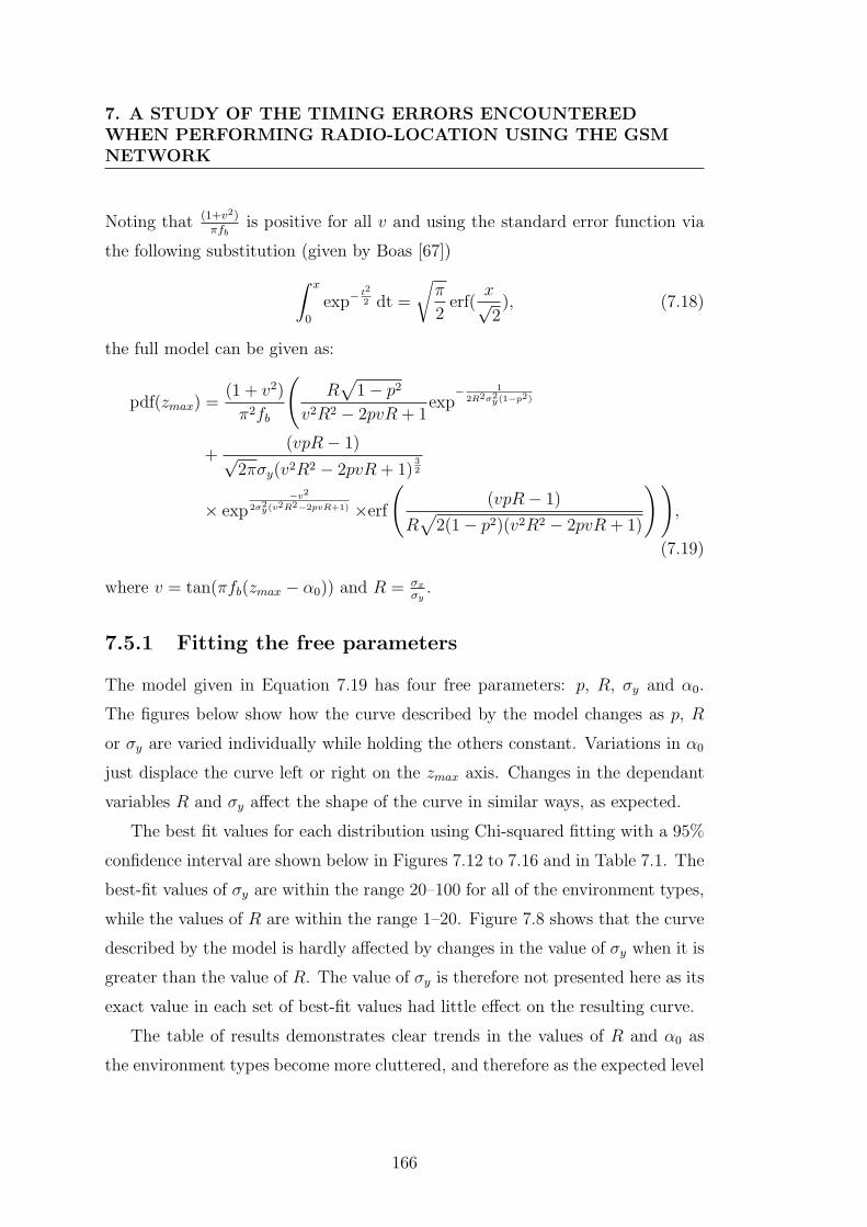
7. A STUDY OF THE TIMING ERRORS ENCOUNTEREDWHEN PERFORMING RADIO-LOCATION USING THE GSMNETWORK
Noting that (1+v2)πfb
is positive for all v and using the standard error function via
the following substitution (given by Boas [67])∫ x
0
exp−t2
2 dt =
√π
2erf(
x√2), (7.18)
the full model can be given as:
pdf(zmax) =(1 + v2)
π2fb
(R√
1− p2
v2R2 − 2pvR + 1exp
− 1
2R2σ2y(1−p2)
+(vpR− 1)
√2πσy(v2R2 − 2pvR + 1)
32
× exp−v2
2σ2y(v2R2−2pvR+1) ×erf
((vpR− 1)
R√
2(1− p2)(v2R2 − 2pvR + 1)
)),
(7.19)
where v = tan(πfb(zmax − α0)) and R = σx
σy.
7.5.1 Fitting the free parameters
The model given in Equation 7.19 has four free parameters: p, R, σy and α0.
The figures below show how the curve described by the model changes as p, R
or σy are varied individually while holding the others constant. Variations in α0
just displace the curve left or right on the zmax axis. Changes in the dependant
variables R and σy affect the shape of the curve in similar ways, as expected.
The best fit values for each distribution using Chi-squared fitting with a 95%
confidence interval are shown below in Figures 7.12 to 7.16 and in Table 7.1. The
best-fit values of σy are within the range 20–100 for all of the environment types,
while the values of R are within the range 1–20. Figure 7.8 shows that the curve
described by the model is hardly affected by changes in the value of σy when it is
greater than the value of R. The value of σy is therefore not presented here as its
exact value in each set of best-fit values had little effect on the resulting curve.
The table of results demonstrates clear trends in the values of R and α0 as
the environment types become more cluttered, and therefore as the expected level
166
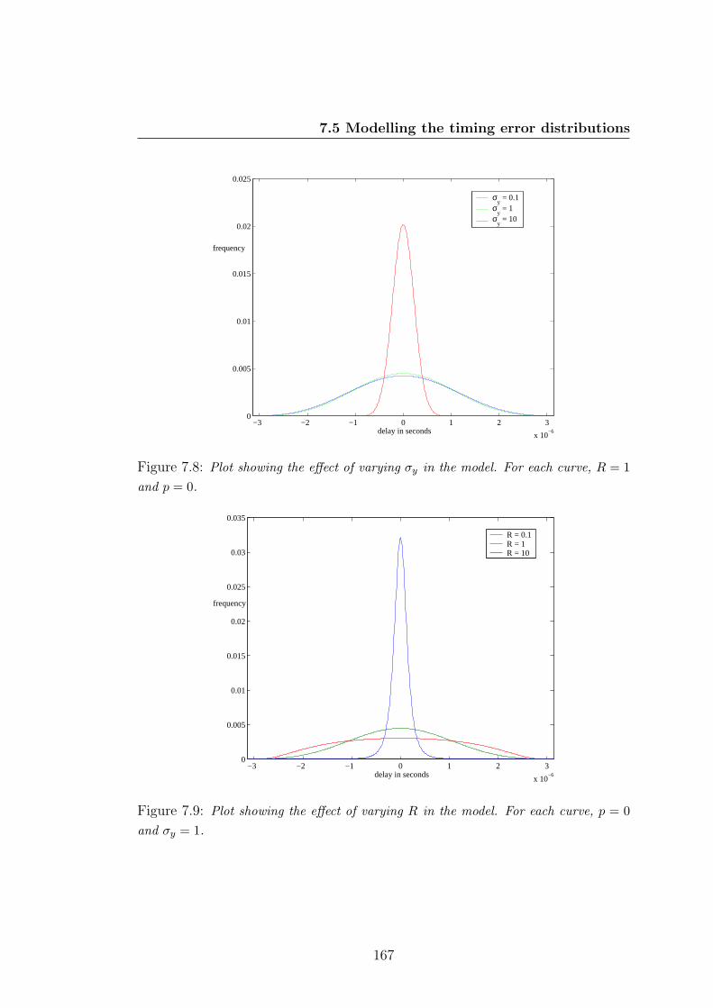
7.5 Modelling the timing error distributions
−3 −2 −1 0 1 2 3
x 10−6
0
0.005
0.01
0.015
0.02
0.025
delay in seconds
frequency
σy = 0.1
σy = 1
σy = 10
Figure 7.8: Plot showing the effect of varying σy in the model. For each curve, R = 1and p = 0.
−3 −2 −1 0 1 2 3
x 10−6
0
0.005
0.01
0.015
0.02
0.025
0.03
0.035
delay in seconds
frequency
R = 0.1R = 1R = 10
Figure 7.9: Plot showing the effect of varying R in the model. For each curve, p = 0and σy = 1.
167
7. A STUDY OF THE TIMING ERRORS ENCOUNTEREDWHEN PERFORMING RADIO-LOCATION USING THE GSMNETWORK
−3−3 −2 −1 0 1 2
x 10−6
0
1
2
3
4
5
6
7
8x 10
−3
delay in seconds
frequency
p = −0.5p = 0p = 0.99
Figure 7.10: Plot showing the effect of varying p in the model. For each curve, R = 1and σy = 1.
Parameter R p α0
Rural 12.7± 1.1 0.03± 0.04 51± 5 ns
Suburban 13.0± 0.1 −0.04± 0.02 72± 6 ns
Light-urban 4.7± 0.3 0.20± 0.12 183± 24 ns
Mid-urban 3.5± 0.3 −0.46± 0.07 239± 23 ns
Indoor 16.0± 3.1 0.54± 0.18 30± 6 ns, 190± 6 ns, 425± 6 ns
Table 7.1: A table showing the best-fit parameters for each dataset.
of multipath interference increases. The values of α0 are useful in determining a
characteristic timing error for each environment, corresponding to the delay of the
earliest-arriving signal in the model. The relationship between these characteristic
delays and the environment types can be estimated using
α0 = 57× E, (7.20)
where E is an integer representing the environment type such that 0 corresponds
to free space, 1 corresponds to rural environments, and so on (see Figure 7.11).
The model fits the rural, suburban, light-urban and mid-urban datasets well,
and its ability to reproduce the experimental results supports the hypothesis
168
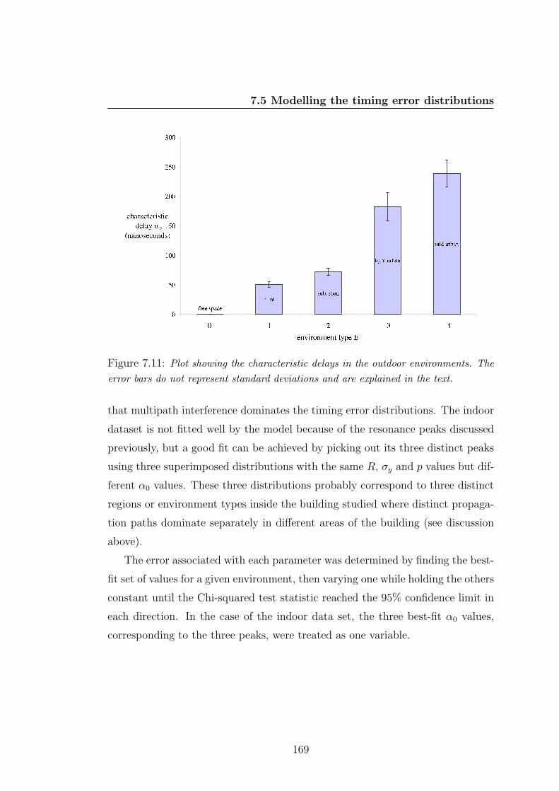
7.5 Modelling the timing error distributions
Figure 7.11: Plot showing the characteristic delays in the outdoor environments. Theerror bars do not represent standard deviations and are explained in the text.
that multipath interference dominates the timing error distributions. The indoor
dataset is not fitted well by the model because of the resonance peaks discussed
previously, but a good fit can be achieved by picking out its three distinct peaks
using three superimposed distributions with the same R, σy and p values but dif-
ferent α0 values. These three distributions probably correspond to three distinct
regions or environment types inside the building studied where distinct propaga-
tion paths dominate separately in different areas of the building (see discussion
above).
The error associated with each parameter was determined by finding the best-
fit set of values for a given environment, then varying one while holding the others
constant until the Chi-squared test statistic reached the 95% confidence limit in
each direction. In the case of the indoor data set, the three best-fit α0 values,
corresponding to the three peaks, were treated as one variable.
169
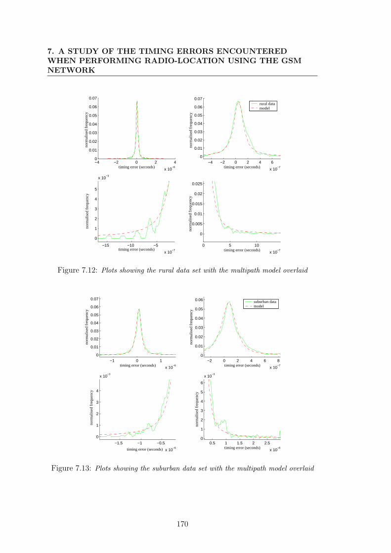
7. A STUDY OF THE TIMING ERRORS ENCOUNTEREDWHEN PERFORMING RADIO-LOCATION USING THE GSMNETWORK
−4 −2 0 2 4
x 10−6
0
0.01
0.02
0.03
0.04
0.05
0.06
0.07
timing error (seconds)
norm
alis
ed f
requ
ency
−4 −2 0 2 4 6
x 10−7
0
0.01
0.02
0.03
0.04
0.05
0.06
0.07
timing error (seconds)
norm
alis
ed f
requ
ency
−15 −10 −5
x 10−7
0
1
2
3
4
5
x 10−3
timing error (seconds)
norm
alis
ed f
requ
ency
0 5 10
x 10−7
0
0.005
0.01
0.015
0.02
0.025
timing error (seconds)
norm
alis
ed f
requ
ency
rural datamodel
Figure 7.12: Plots showing the rural data set with the multipath model overlaid
−1 0 1
x 10−6
0
0.01
0.02
0.03
0.04
0.05
0.06
0.07
timing error (seconds)
norm
alis
ed f
requ
ency
−2 0 2 4 6 8
x 10−7
0
0.01
0.02
0.03
0.04
0.05
0.06
timing error (seconds)
norm
alis
ed f
requ
ency
−1.5 −1 −0.5
x 10−6
0
1
2
3
4
x 10−3
timing error (seconds)
norm
alis
ed f
requ
ency
0.5 1 1.5 2 2.5
x 10−6
0
1
2
3
4
5
6
x 10−3
timing error (seconds)
norm
alis
ed f
requ
ency
suburban datamodel
Figure 7.13: Plots showing the suburban data set with the multipath model overlaid
170
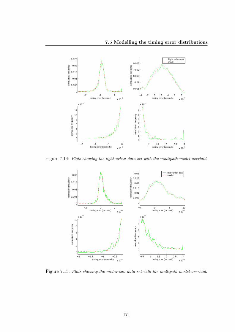
7.5 Modelling the timing error distributions
−2 0 2
x 10−6
0
0.005
0.01
0.015
0.02
0.025
timing error (seconds)
norm
alis
ed fr
eque
ncy
−4 −2 0 2 4 6 8
x 10−7
0.005
0.01
0.015
0.02
0.025
timing error (seconds)
norm
alis
ed fr
eque
ncy
−3 −2 −1 0
x 10−6
0
2
4
6
8
10
12
x 10−3
timing error (seconds)
norm
alis
ed fr
eque
ncy
1 1.5 2 2.5 3
x 10−6
0
1
2
3
4
5
6
7
x 10−3
timing error (seconds)
norm
alis
ed fr
eque
ncy
light−urban datamodel
Figure 7.14: Plots showing the light-urban data set with the multipath model overlaid.
−2 0 2
x 10−6
0
0.005
0.01
0.015
0.02
timing error (seconds)
norm
alis
ed fr
eque
ncy
−5 0 5 10
x 10−7
0
0.005
0.01
0.015
0.02
0.025
0.03
timing error (seconds)
norm
alis
ed fr
eque
ncy
−2 −1.5 −1 −0.5
x 10−6
0
2
4
6
8
10x 10
−3
timing error (seconds)
norm
alis
ed fr
eque
ncy
0.5 1 1.5 2 2.5 3
x 10−6
0
2
4
6
8
x 10−3
timing error (seconds)
norm
alis
ed fr
eque
ncy
mid−urban datamodel
Figure 7.15: Plots showing the mid-urban data set with the multipath model overlaid.
171
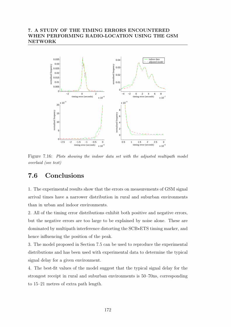
7. A STUDY OF THE TIMING ERRORS ENCOUNTEREDWHEN PERFORMING RADIO-LOCATION USING THE GSMNETWORK
−2 0 2
x 10−6
0
0.005
0.01
0.015
0.02
0.025
0.03
0.035
timing error (seconds)
norm
alis
ed f
requ
ency
−4 −2 0 2 4 6 8
x 10−7
0
0.01
0.02
0.03
0.04
timing error (seconds)
norm
alis
ed f
requ
ency
−2.5 −2 −1.5 −1 −0.5 0
x 10−6
0
5
10
15
20x 10
−3
timing error (seconds)
norm
alis
ed f
requ
ency
0.5 1 1.5 2 2.5 3
x 10−6
0
2
4
6
8
x 10−3
timing error (seconds)
norm
alis
ed f
requ
ency
indoor dataadjusted model
Figure 7.16: Plots showing the indoor data set with the adjusted multipath modeloverlaid (see text)
7.6 Conclusions
1. The experimental results show that the errors on measurements of GSM signal
arrival times have a narrower distribution in rural and suburban environments
than in urban and indoor environments.
2. All of the timing error distributions exhibit both positive and negative errors,
but the negative errors are too large to be explained by noise alone. These are
dominated by multipath interference distorting the SCB?ETS timing marker, and
hence influencing the position of the peak.
3. The model proposed in Section 7.5 can be used to reproduce the experimental
distributions and has been used with experimental data to determine the typical
signal delay for a given environment.
4. The best-fit values of the model suggest that the typical signal delay for the
strongest receipt in rural and suburban environments is 50–70ns, corresponding
to 15–21 metres of extra path length.
172
7.6 Conclusions
5. The best-fit values of the model suggest that an extra signal delay of 180–240
nanoseconds is a feature of urban environments, corresponding to 55–72 metres
of apparent extra path length. However, the modelling performed in Chapter 6
suggests that moderate and dense multipath interference results in a bias toward
positive timing errors (see the peak-position histograms in Figures 6.11 and 6.10).
In either case, the result is an effective typical signal delay value of around 200
nanoseconds in these environments.
6. A simple ‘rule of thumb’ equation is proposed to allow the characteristic delay
for a given environment type to be estimated using a simple calculation.
7. The indoor environment showed a different error distribution from the outdoor
environments, and cannot be accurately modelled using the model as given by
Equation 7.19 above. However, a good fit can be achieved by superimposing 3
curves described by the model with different values of α0, the variable correspond-
ing to the delay of the earliest significant arrival. This would suggest a number
of different propagation mechanisms active in the environment and each domi-
nating in different areas depending on the exact nature of the local environment,
i.e. being near a window, or in a long corridor, etc.
173
7. A STUDY OF THE TIMING ERRORS ENCOUNTEREDWHEN PERFORMING RADIO-LOCATION USING THE GSMNETWORK
174
Chapter 8
Summary and further work
8.1 The experimental apparatus
A set of apparatus was constructed in order to measure signal arrival times via the
SCB broadcasts on the BCCH channels of base stations on the GSM network. The
140 kHz-bandwidth GSM broadcasts were oversampled, allowing the signals to be
fully reconstructed using the Nyquist-Shannon sampling theory. The signals were
sampled at a rate of 2.04 MHz and interpolated to increase this resolution by a
factor of 20 to allow an effective timing resolution of 24.5 nanoseconds. In practise,
the accuracy of an individual recording was decreased by measurement noise and
temporal multipath interference, but averaging over many measurements reduced
the effect of these errors. Systematic errors from features such as the instabilities
of the frequency references were discussed and quantified. They were found to be
insignificant over short experiments lasting a few hours.
8.2 The experimental methods
Two experimental methods were proposed, the interferometric method and the
network-synchronised method. The interferometric method removed systematic
errors caused by fluctuations in the base station broadcasts, whereas the network-
175
8. SUMMARY AND FURTHER WORK
synchronised method required half as much equipment and only one operator.
The accuracy of the network-synchronised method approached the accuracy of the
interferometric approach as the stability of the base station frequency standards
increased.
8.3 GSM network timing stabilities
The temporal stability of the received signals on two GSM networks were mea-
sured. The signals broadcasted by the base stations on Network 1 all demon-
strated a very high level of stability, leading to the conclusion that the network-
synchronised method could be used with this network. The temporal stability
of a received signal was noted to reduce for an indoor antenna, demonstrating
that the received temporal stability was dependant not only on the base sta-
tion’s frequency standard, but also on the propagation path and signal strength.
The signals on Network 2 all demonstrated a reduced stability when compared
to Network 1. Three distinct signal qualities were observed during the exper-
iments, which were assumed to have been caused by the different technologies
and frequency-stabilising techniques used in base stations of different ages and
on different networks. The results of the experiments suggested that Network
1 could be used confidently to provide FTA to an E-GPS device with periods
of 3 days or more between calibrations, whereas Network 2 could only be used
confidently to provide FTA with periods of 5 hours or less between calibrations.
8.4 GSM network timing stabilities in indoor
multipath environments
The multipath behaviour over sub-wavelength distances indoors was studied. Sig-
nificant timing errors of a microsecond or more were recorded for antenna move-
176
8.5 GSM radio location timing error distributions in variousenvironments
ments on the millimetre scale. This behaviour was also noted during an experi-
ment with a visible line of sight to the base station in an outdoor but cluttered
environment, confirming that extreme errors due to multipath can still occur
even with a line of sight between a transmitter and receiver. A model based
on superimposing truncated raised-cosine functions was proposed to simulate the
superposition of the SCB peaks from interfering multipath signals. The model
was shown to reproduce features seen in the experimental results. Two methods
were proposed for increasing the accuracy of determining signal arrival times, the
peak-rise method and the midpoint method. Both methods improved the tim-
ing accuracy by removing the most extreme errors in a given data set, but both
required more intensive computation than the simple peak-max technique.
8.5 GSM radio location timing error distribu-
tions in various environments
The timing error distributions in various environments were determined by us-
ing the peak-max technique to measure signal flight times on the GSM network.
The timing error distributions in rural and suburban environments were narrower
than for urban and indoor environments, and were also reasonably symmetrical
about zero. The urban and indoor distributions were not symmetrical about zero,
containing more positive timing error values than negative. This suggested that
there is either a mean, non-zero signal delay in these environment types, or that
moderate and dense multipath interference results in a bias toward positive tim-
ing errors. The modelling performed during the indoor multipath experiments
suggested that the latter may be true, but in either case, the result was an effec-
tive mean or ‘typical’ signal delay value in these environments. A timing error
probability density function model was derived from the raised-cosine model and
was shown to reproduce the experimental distributions. The model reproduced
177
8. SUMMARY AND FURTHER WORK
the urban datasets best when an extra path delay of 180–240 nanoseconds was
included, suggesting that the signals in these environments have a typical ex-
tra path length of 55-72 metres. The indoor timing-error distribution exhibited
three distinct peaks, corresponding to three distinct groups of signals with dif-
ferent mean propagation delays. This feature was possibly caused by signals
resonating in the building’s corridors, or by signals entering the test environment
after reflecting from different local buildings.
8.6 Further work
The network stability measurements discussed in Chapter 4 were only performed
on two networks, and only in Cambridge, England. This was adequate for the
purposes of determining whether the network-synchronised technique could be
used during this research, but further network stability tests are required to de-
termine more accurate figures relating to the capability of GSM networks to pro-
vide FTA. The degradation in timing stability experienced by a rapidly moving
receiver (such that Doppler effects are not negligible) should also be investigated
to determine the effect on providing FTA to a moving receiver. Further investi-
gations into new techniques for determining signal arrival times using the SCB
cross-correlation peak should also be carried out, as they can improve the accu-
racy of GSM radio positioning and as the processing power of handsets increase,
computation-hungry algorithms will become a viable option. The timing error
distribution for a dense urban environment such as the centre of London still
needs to be determined.
Finally, performing the experiments discussed in Chapters 4–6 of this thesis
on the 3G network would be an appropriate large-scale extension to this work.
The much shorter coherence length of these wide-band signals would yield a much
finer resolution and so provide much more information about the multipath envi-
ronment. The TOA estimation methods would therefore also be different and are
178
8.6 Further work
worth researching. The actual mechanisms of radio positioning on 3G networks
can also be researched, as this is not a simple task using CDMA signals. The
signals are all broadcast in the same waveband, and so strong local signals over-
power weaker distant signals. Radio positioning typically requires measurements
from at least three base stations, but it is difficult to perform measurements using
a number of base stations simultaneously using the 3G network. Techniques such
as Cumulative Virtual Blanking [68] need to be developed.
179

8. SUMMARY AND FURTHER WORK
180
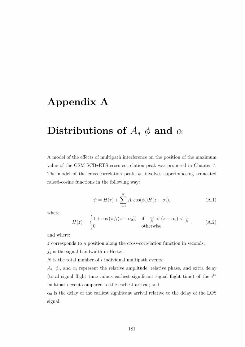
Appendix A
Distributions of A, φ and α
A model of the effects of multipath interference on the position of the maximum
value of the GSM SCB?ETS cross correlation peak was proposed in Chapter 7.
The model of the cross-correlation peak, ψ, involves superimposing truncated
raised-cosine functions in the following way:
ψ = H(z) +N∑i=1
Ai cos(φi)H(z − αi), (A.1)
where
H(z) =
1 + cos (πfb(z − α0)) if −1
fb< (z − α0) <
1fb
0 otherwise, (A.2)
and where:
z corresponds to a position along the cross-correlation function in seconds;
fb is the signal bandwidth in Hertz;
N is the total number of i individual multipath events;
Ai, φi, and αi represent the relative amplitude, relative phase, and extra delay
(total signal flight time minus earliest significant signal flight time) of the ith
multipath event compared to the earliest arrival; and
α0 is the delay of the earliest significant arrival relative to the delay of the LOS
signal.
181
A. DISTRIBUTIONS OF A, φ AND α
The model also involves the two summation terms,
S1 =N∑i=0
Ai cos(φi) sin(πfbαi) (A.3)
and
S2 = 1 +N∑i=0
Ai cos(φi) cos(πfbαi). (A.4)
The central limit theorem [65] states that any summation will tend toward a
normal distribution as N tends to infinity if the variables being summed are
all randomly chosen, independent, and are drawn from distributions with finite
variances. The values of A, φ and α fit these criteria, but the condition for N
being large enough needs to be determined. There is also a clear dependency
between S1 and S2, suggesting that their limiting Gaussian distributions will not
be independent.
The validity of applying the central limit theorem here can be determined by
using suitable distributions of A, φ and α to calculate many values of S1 and S2
to see if they are normally distributed. The distributions of A, φ and α cannot
be determined but they can be estimated.
A.1 Distribution of φ
The distribution of φ is dependant on two major features:
1. The reflection, diffraction, refraction, and scattering processes, which give rise
to many signals arriving at a given point via different paths, change a given sig-
nal’s phase such that it no longer depends on the path length alone.
2. For a GSM signal with a central frequency of around 900MHz and a band-
width of 140 kHz, the value of φ changes over its full range as the receiver is
moved about 30 centimetres along the line of propagation. The amplitude of the
individual signal (Ai) and the value of πfbαi will change negligibly by comparison
over this small distance.
182
A.2 Distribution of α
Taking these two features together suggests that modelling φ with a uniform dis-
tribution between −π and π independent of α is appropriate, i.e. the probability
density function (pdf) of φ can be given as:
pdf(φ) =1
2π, for − π ≤ φ ≤ π. (A.5)
A.2 Distribution of α
The distribution of α represents the signals which arrive at the receiver with
significant amplitudes, since delayed paths with negligible corresponding ampli-
tudes do not contribute to the multipath interference being modelled. Therefore,
α cannot be negative (since the LOS signal is always represented by α = 0) and
the probability density function must tail-off as the value of α increases, since
the likelihood of a significant signal decreases with increasing delay. A suitable
distribution based on these criteria is a Rayleigh distribution, given by:
pdf(α) =α
σ2α
exp−α2
σ2α , for 0 ≤ α ≤ ∞, (A.6)
where the parameter σα determines the modal value of the distribution.
A.3 Distribution of A
Estimating the distribution of signal amplitudes involves considering the signal
propagation mechanisms. At GSM frequencies, the signals can penetrate and
propagate through buildings and other objects such that even when the LOS
path is visibly obstructed the attenuated LOS signal could still be part of the
multipath environment, but possibly with a lower amplitude than one or more of
the multipath signals. In this model the value of A is defined such that the ampli-
tude of the LOS receipt or earliest significant signal arrival is always normalised
to 1. Therefore when modelling rural and suburban environment positions where
183
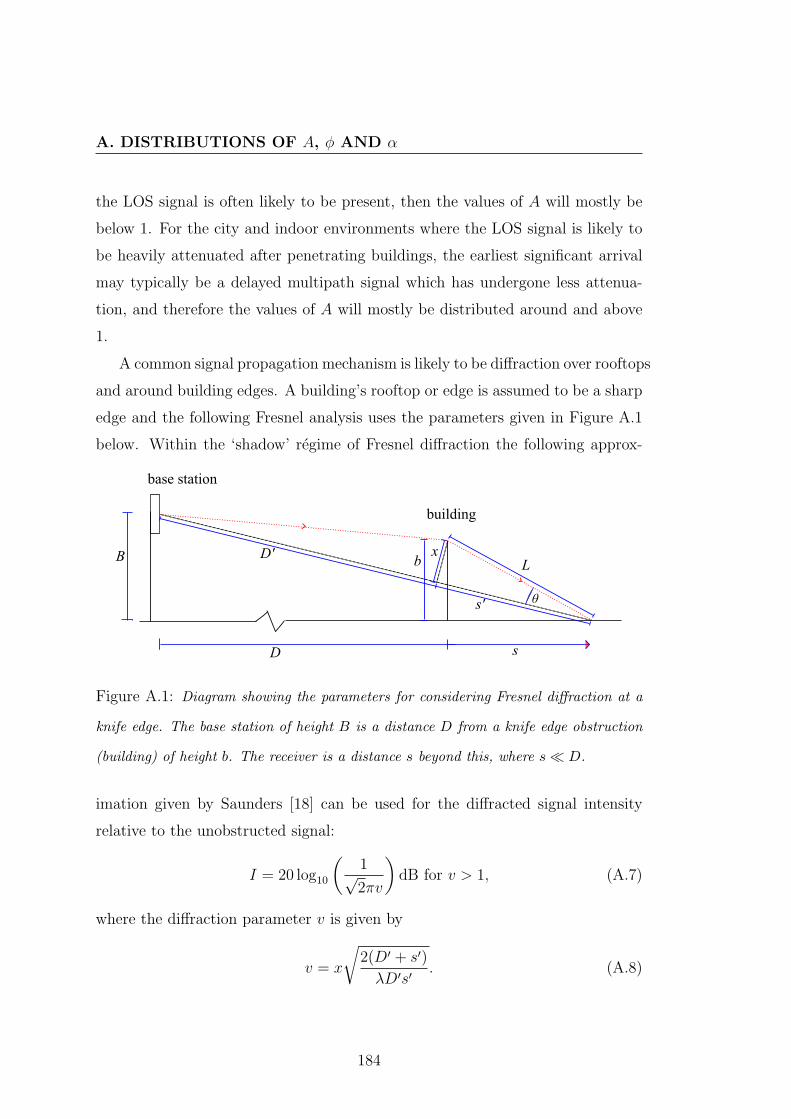
A. DISTRIBUTIONS OF A, φ AND α
the LOS signal is often likely to be present, then the values of A will mostly be
below 1. For the city and indoor environments where the LOS signal is likely to
be heavily attenuated after penetrating buildings, the earliest significant arrival
may typically be a delayed multipath signal which has undergone less attenua-
tion, and therefore the values of A will mostly be distributed around and above
1.
A common signal propagation mechanism is likely to be diffraction over rooftops
and around building edges. A building’s rooftop or edge is assumed to be a sharp
edge and the following Fresnel analysis uses the parameters given in Figure A.1
below. Within the ‘shadow’ regime of Fresnel diffraction the following approx-
Figure A.1: Diagram showing the parameters for considering Fresnel diffraction at a
knife edge. The base station of height B is a distance D from a knife edge obstruction
(building) of height b. The receiver is a distance s beyond this, where s D.
imation given by Saunders [18] can be used for the diffracted signal intensity
relative to the unobstructed signal:
I = 20 log10
(1√2πv
)dB for v > 1, (A.7)
where the diffraction parameter v is given by
v = x
√2(D′ + s′)
λD′s′. (A.8)
184
A.3 Distribution of A
The parameters x, D′ and s′ are given above in Figure A.1. It can also be shown
using the diagram that:
s′ = L cos(θ), (A.9)
D′ =√
(D + s)2 +B2 − s′, (A.10)
sin(θ) =x
L, (A.11)
and
L =√s2 + b2, (A.12)
and so
x =(√
s2 + b2)
sin
(arctan
(b
s
)− arctan
(B
D + s
)). (A.13)
The signal intensity, I (in dB), is converted to amplitude (in linear units) via the
relationship:
A = A010I10 . (A.14)
Plots of the resulting signal amplitude versus distance from the base of the point
of diffraction are given in Figure A.2 below. The signal amplitudes are given as
the value relative to the unobstructed free space amplitude at each point. In or-
der to generate a probability density function for this mechanism, the histogram
of the values given by one of these curves can be considered. The distribution
of A for a particular building size and BTS distance would then be given by a
function that fits this histogram. However, since a general distribution of A is
required, it is better to generate A values using the Fresnel diffraction model for
randomly drawn environmental parameters and therefore create a more general
histogram. This distribution of A will be valid for the case where a single diffrac-
tion over rooftops or around the edges of buildings can be argued to be a dominant
propagation mechanism, such as may be the case in urban environments.
185
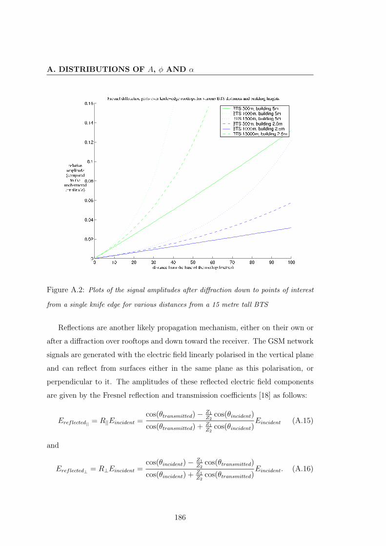
A. DISTRIBUTIONS OF A, φ AND α
Figure A.2: Plots of the signal amplitudes after diffraction down to points of interest
from a single knife edge for various distances from a 15 metre tall BTS
Reflections are another likely propagation mechanism, either on their own or
after a diffraction over rooftops and down toward the receiver. The GSM network
signals are generated with the electric field linearly polarised in the vertical plane
and can reflect from surfaces either in the same plane as this polarisation, or
perpendicular to it. The amplitudes of these reflected electric field components
are given by the Fresnel reflection and transmission coefficients [18] as follows:
Ereflected|| = R||Eincident =cos(θtransmitted)− Z1
Z2cos(θincident)
cos(θtransmitted) + Z1
Z2cos(θincident)
Eincident (A.15)
and
Ereflected⊥ = R⊥Eincident =cos(θincident)− Z1
Z2cos(θtransmitted)
cos(θincident) + Z1
Z2cos(θtransmitted)
Eincident. (A.16)
186
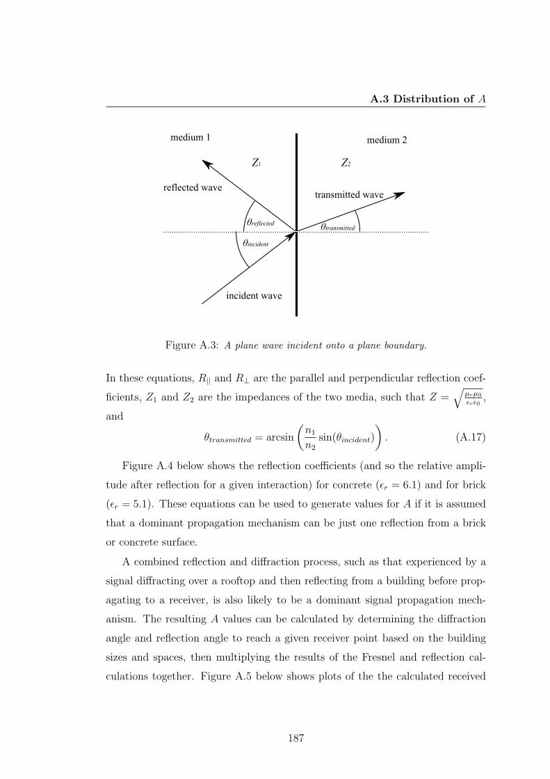
A.3 Distribution of A
Figure A.3: A plane wave incident onto a plane boundary.
In these equations, R|| and R⊥ are the parallel and perpendicular reflection coef-
ficients, Z1 and Z2 are the impedances of the two media, such that Z =√
µrµ0
εrε0,
and
θtransmitted = arcsin
(n1
n2
sin(θincident)
). (A.17)
Figure A.4 below shows the reflection coefficients (and so the relative ampli-
tude after reflection for a given interaction) for concrete (εr = 6.1) and for brick
(εr = 5.1). These equations can be used to generate values for A if it is assumed
that a dominant propagation mechanism can be just one reflection from a brick
or concrete surface.
A combined reflection and diffraction process, such as that experienced by a
signal diffracting over a rooftop and then reflecting from a building before prop-
agating to a receiver, is also likely to be a dominant signal propagation mech-
anism. The resulting A values can be calculated by determining the diffraction
angle and reflection angle to reach a given receiver point based on the building
sizes and spaces, then multiplying the results of the Fresnel and reflection cal-
culations together. Figure A.5 below shows plots of the the calculated received
187
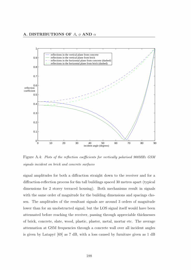
A. DISTRIBUTIONS OF A, φ AND α
0 10 20 30 40 50 60 70 80 900
0.1
0.2
0.3
0.4
0.5
0.6
0.7
0.8
0.9
1
incident angle (degrees)
reflectioncoefficient
reflections in the vertical plane from concrete reflections in the vertical plane from brickreflections in the horizontal plane from concrete (dashed)reflections in the horizontal plane from brick (dashed)
Figure A.4: Plots of the reflection coefficients for vertically polarised 900MHz GSM
signals incident on brick and concrete surfaces
signal amplitudes for both a diffraction straight down to the receiver and for a
diffraction-reflection process for 6m tall buildings spaced 30 metres apart (typical
dimensions for 2 storey terraced housing). Both mechanisms result in signals
with the same order of magnitude for the building dimensions and spacings cho-
sen. The amplitudes of the resultant signals are around 3 orders of magnitude
lower than for an unobstructed signal, but the LOS signal itself would have been
attenuated before reaching the receiver, passing through appreciable thicknesses
of brick, concrete, slate, wood, plastic, plaster, metal, mortar etc. The average
attenuation at GSM frequencies through a concrete wall over all incident angles
is given by Latapyc [69] as 7 dB, with a loss caused by furniture given as 1 dB
188
A.3 Distribution of A
per metre. Therefore for a typical small house, assuming one internal wall and
a few metres of furniture, a loss of around 25 dB might be expected for a path
through the building. This corresponds to a change in amplitude to a factor of
0.003 of its initial value, which is similar to the values for the other propagation
mechanisms.
Scattering processes from poles, posts, branches and rough surfaces will also
provide signal propagation mechanisms. When the scattering object has a dimen-
sion comparable to the wavelength of the radiation (which is true for poles, posts,
window ledges, branches, tree trunks, etc, at GSM frequencies.) the scattering
will be most effective. According to the “effective roughness” approach presented
by Esposti [70, 71], the adjusted Lambertian model for diffuse scattering from a
surface is given by
Es =K · Sri · rs
√√√√ 8 · dS · cos(θi)
4π + 3π · cos(θi) ·(1 + sin2 θi
4
)+ π
2· cos3 θi
·
(1− (sin θs · sin θi) · cos (φs − φi) + cos θi · cos θs
2
) 32
, (A.18)
where S is the scattering coefficient, dS is the surface element scattering radiation,
(ri, θi, φi) are the polar coordinates of the incident wave, Es is the amplitude of
the scattered wave at polar coordinate (rs, θs, φs), and K is a constant dependant
on the amplitude of the impinging radiation. Values can be drawn from this
model using random coordinates and coefficients in order to generate a probability
density function for this propagation mechanism as before.
Free-space path-loss is an important factor in attenuating the signal over a
long propagation path, but the attenuation caused by the slightly increased path
length due to a reflection, diffraction or scatter is negligible compared to the
attenuation caused by the signal deflection interaction. The effects of free space
path loss due to the slightly increased path lengths caused by these propagation
mechanisms is therefore ignored.
189
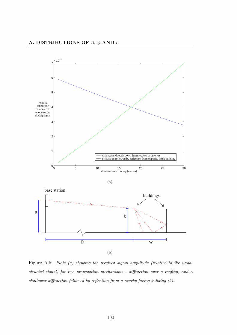
A. DISTRIBUTIONS OF A, φ AND α
0 5 10 15 20 25 300
1
2
3
4
5
6
7x 10
−3
relativeamplitude
compared tounobstructed(LOS) signal
distance from rooftop (metres)
diffraction directly down from rooftop to receiverdiffraction followed by reflection from opposite brick building
(a)
(b)
Figure A.5: Plots (a) showing the received signal amplitude (relative to the unob-
structed signal) for two propagation mechanisms - diffraction over a rooftop, and a
shallower diffraction followed by reflection from a nearby facing building (b).
190
A.3 Distribution of A
These four propagation mechanisms all result in different probability distri-
butions for A, but the aim of this exercise is to verify whether the sums S1 and
S2 described above tend to Gaussian distributions as the number of terms in
the sums increases, so checking this for all four potential distributions for A will
determine if the use of the Gaussian approximation is valid.
A large number of values for S1 and S2 were calculated using the distribu-
tions of α, φ and the four propagation mechanisms given above to represent four
possible distributions of A. The following figures show the resulting plots for
each distribution of A, assuming 10 multipath interactions per point of interest
(i.e. N = 10 in the sums S1 and S2) - a reasonable value considering the number
of surfaces and edges available in a typical multipath environment. Each plot
consists of 120,000 values of S1 and S2 and a bivariate Gaussian distribution is
overlaid for comparison. All four plots support the use of the central limit the-
orem approximation for these distributions and 10 multipath events per survey
point.
————————————————————————
191
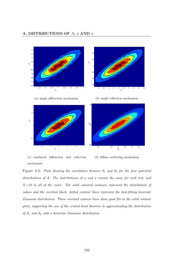
A. DISTRIBUTIONS OF A, φ AND α
1.25 1.5 1.75 2 2.25 2.5 2.75 30.75
0.8
0.85
0.9
0.95
1
1.05
1.1
1.15
1.2
S2
S1
(a) single diffraction mechanism
0 0.5 1 1.5 2 2.5 3 3.5 4 4.5
0.4
0.6
0.8
1
1.2
1.4
S2
S1
(b) single reflection mechanism
0 1 2 3 4 5
0.5
1
1.5
S2
S1
(c) combined diffraction and reflection
mechanism
(d) diffuse scattering mechanism
Figure A.6: Plots showing the correlation between S1 and S2 for the four potential
distributions of A. The distributions of α and φ remain the same for each test, and
N=10 in all of the sums. The solid coloured contours represent the distribution of
values and the overlaid black, dotted contour lines represent the best-fitting bivariate
Gaussian distribution. These overlaid contour lines show good fits to the solid contour
plots, supporting the use of the central limit theorem in approximating the distribution
of S1 and S2 with a bivariate Gaussian distribution
192
Bibliography
[1] K. B. Williams. Secret Weapon: US High-Frequency Direction Finding in
the Battle of the Atlantic. Naval Inst Pr, 1996. 1.1
[2] 2001 Federal Radionavigation systems. United States Department of De-
fense and Department of Transportation, DOT-VNTSC-RSPA-01-3.1/DOD-
4650.5, 2001. 1.1, 1.1
[3] A. Price. Instruments of Darkness: The History of Electronic Warfare.
Peninsula, 1977. 1.1
[4] J. A. Pierce. Omega: Facts, Hopes and Dreams. Harvard University of
Cambridge, Department of Engineering and Applied Physics, 1974. 1.1
[5] N. Bowditch. The American Practical Navigator. National Imagery and
Mapping Agency, 2002. 1.1
[6] Wireless Intelligence. www.cellular-news.com/story/19223.php. 1.2
[7] P. Solanki and H. Huosheng. Techniques used for location-based services: A
survey. Master’s thesis, University of Essex, 2005. 1.2.1
[8] PPS 10 Telecommunications. www.planningni.gov.uk. 1.2.1
[9] P. Kemppi. Database correlation method for multi-system location. Master’s
thesis, Helsinki University of Technology, 2005. 1.2.2
193
BIBLIOGRAPHY
[10] G. Wolfle, R. Hoppe, D. Zimmermann, and F. M. Landstorfer. Enhanced
localization technique within urban and indoor environments based on accu-
rate and fast propagation models. European Wireless 2002, Firence, Italy:7,
February 2002. 1.2.2
[11] V. Otsason. Accurate indoor localization using wide GSM fingerprinting.
Master’s thesis, University of Tartu, 2005. 1.2.2
[12] Location Based Services. GSM Association Permanent Reference Document
SE 2.3, ver 3.1.0:52, 2003. 1.2.3
[13] P. J. Duffett-Smith, J. P. Brice, and P. Hansen. Radio positioning systems.
US Patent Number 6,529,165, 4th March 2003. 1.2.4
[14] P. J. Duffett-Smith and J. P. Brice. Positioning systems and methods. US
Patent Number 6,937,866, 30th August 2005. 1.2.4
[15] C. Drane, P. J. Duffett-Smith, S. Hern, and J. P. Brice. Mobile positioning
using E-OTD without LMUs. proceedings of AeroSense 2003, SPIE’s 17th
Annual International Symposium on Aerospace/Defence Sensing, Simulation
and Controls, 2003. 1.2.4
[16] Duffett-Smith P. J. and B. Tarlow. E-GPS: indoor mobile phone positioning
on GSM and W-CDMA. Proceedings of the ION GNSS 2005, Long Beach,
September 2005. 1.2.5, 4.2.1
[17] N. Blaunstein and J. B. Andersen. Multipath phenomena in cellular networks.
Artech House, 2002. 1.3, 1.4
[18] S. R. Saunders. Antennas and Propagation for Wirelss Communication Sys-
tems. Wiley, 1999. 1.4, A.3, A.3
[19] J. Borkowski and J. Lempiainen. Geometrical transformations as an efficient
mean for reducing impact of multipath propagation on positioning accuracy.
194
BIBLIOGRAPHY
Proceedings of the IEE International Conference on 3G Mobile Communica-
tion Technologies, pages 368–372, October 2004. 1.4
[20] T. Rautiainen, G. Wolfle, and R. Hoppe. Verifying path loss and delay spread
predictions of a 3d ray tracing propagation model in urban environment.
Vehicular Technology Conference, 2002, IEEE VTC 56th, 4:2470–2474, 2004.
1.4
[21] M. J. Mughal, A. M. Street, and C. C. Constantinou. Detailed radio imaging
of buildings at 2.4 GHz. Vehicular Technology Conference, 2000, IEEE VTC
52nd, 1:57–63, 2000. 1.4
[22] G. Wolfle, R. Hoppe, D. Zimmerman, and Landstorfer F. Enhanced local-
ization technique within urban and indoor environments based on accurate
and fast propagation models. European Wireless, 2002. 1.4
[23] A. R. Thompson, J. M. Moran, and G. W. Swenson, Jr. Interferometry and
Synthesis in Radio Astronomy. Wiley, 1986. 2.1, 2.1, 2.2, 2.11
[24] D. W Allan. Statistics of atomic frequency standards. Proceedings of the
IEEE, 54:221–230, 1966. 2.1
[25] P. Lesage and C. Audoin. Characterization and measurement of time and
frequency stability. Radio Sci., 14:521–539, 1979. 2.1
[26] J. A. Barnes. Atomic time keeping and the statistics of precision signal
generators. Proc. IEEE, 54:207–219, 1966. 2.1
[27] D. W. Allan, N. Ashby, and C. C. Hodge. The science of timekeeping.
Hewlett Packard Application Note 1289. 2.1, 2.1
[28] R. F. C. Vessot. Frequency and time standards. Methods of Experimental
Physics, 12C:198–227, 1976. 2.1, 2.1
195
BIBLIOGRAPHY
[29] N. F. Ramsey. The Atomic Hydrogen Maser. Metrologia, 1:7–15, 1965. 2.4,
2.1, 2.3.3
[30] Clairon et al. The LPTF Preliminary Accuracy Evaluation of Cesium Foun-
tain Frequency Standard. Proceedings of Tenth European Frequency and
Time Forum, 1:218–223, 1996. 2.4, 2.1, 2.3.4
[31] D. Boiron, A. Michaud, P. Lemonde, and Y. Castin. Laser cooling of Cesium
atoms in gray optical molasses down to 1.1µk. Phys. Rev. A., 53:R3734–
R3737, 1996. 2.4, 2.1
[32] A. Di Stephano, D. Wilkowski, J. H. Muller, and E. Arimondo. Five-beam
magneto-optical trap and optical molasses. Applied Physics. B, Lasers and
optics, 69:263–268, 1999. 2.4, 2.1
[33] S. A. Diddams, Th. Udem, J. C. Bergquist, E. A. Curtis, R. E. Drullinger,
L. Hollberg, W. M. Itano, W. D. Lee, and C. W. Oates. An Optical Clock
based on a single trapped 199Hg+ ion. Science, 293:825–828, 2001. 2.4, 2.1,
2.3.5
[34] M. Takamoto, F. Hong, R. Higashi, and H. Katori. An optical lattice clock.
Nature, 435:321–324, 2005. 2.4, 2.1, 2.3.5
[35] S. T. Cundiff and J. Ye. Colloquium: Femtosecond optical frequency combs.
Rev. Mod. Phys., 75:325–342, 2003. 2.4, 2.1, 2.3.5
[36] E. Beehler, R., R. C. Mockler, and J. M. Rischardson. Cesium Beam Atomic
Time and Frequency Standards. Metrologia, 1:114–131, 1965. 2.1, 2.3.2
[37] K. C. A. Smith and R. E. Alley. Electrical Circuits. Cambridge University
Press, 1992. 2.2
[38] D. Biddulph. Radio Communication Handbook. Radio Society of Great
Britain, 1994. 2.2
196
BIBLIOGRAPHY
[39] J. C. Brice. Crystals for quartz resonators. Rev. Mod. Phys., 57:105–146,
1985. 2.2.1
[40] J. R. Vig. Introduction to Quartz Frequency Standards. Army Research
Laboratory EPSD, SLCETTR921, 1992. 2.10
[41] E. Frerking, M. Crystal oscillator design and temperate compensation. Van
Norstrand Reinhold, New York, 1978. 2.2.2
[42] OCXOs Oven Controlled Crystal Oscillators. Vectron International Appli-
cation Note. 2.2.3
[43] M. Bloch, M. Myers, and J. Ho. The microcomputer compensated crystal
oscillator (MCXO). Proceedings of the 43rd Annual Symposium on Frequency
Control, pages 16–19, 1989. 2.2.4
[44] B. H. Bransden and C. J. Jochain. Physics of Atoms and Molecules. Prentice
Hall, 1996. 2.3.1, 2.3.1
[45] P. Zeeman. On the influence of magnetism on the nature of light emitted by
a substance. Philosophical Magazine, 43:226, 1897. 2.3.1
[46] C. Audoin and J. Vanier. Atomic frequency standards and clocks. Journal
of Physics E: Scientific Instruments, 9:697–720, 1979. 2.3.1
[47] A. Kastler. Quelques questions concernant la production optique du inegalite
du population des niveaux qualification spatiale des atoms. Application a
l’experience de Stern et Gerlach et a la resonance magnetique. J. Phys.
Radium (France), 11:255–265, 1950. 2.3.1
[48] P. L. Bender, E. C. Beaty, and A. R. Chi. Optical detection of narrow Rb87
hyperfine absorption lines. Phys. Rev., 1:311, 1958. 2.3.1
[49] P. Davidovits and R. Novick. The optically-pumped Rubidium maser. Proc.
IEEE, 54:155, 1966. 2.3.1
197
BIBLIOGRAPHY
[50] R. H. Dicke. The effect of collisions upon the Doppler width of spectral lines.
Phys. Rev., 89:472, 1953. 2.3.1
[51] P. Forman. Alfred Lande and the anomalous Zeeman effect, 1919-1921.
Historical Studies in the Physical Sciences, 2:153–261, 1970. 2.3.1
[52] 13th General Conference of Weights and Measures. CGPM [Conference Gen-
erale des Poids et Mesures] Resolution 1). 2.3.2
[53] N. F. Ramsey. Molecular Beams. Oxford: Clarendon, 1956. 2.3.2
[54] http://www.quartzlock.com/resources/ANQL1 02.pdf. 2.3.3
[55] IFR 2319E data sheet. www.aeroflex.com. 3.2.1
[56] C. E. Shannon. Communication in the presence of noise. Proc. Institute of
Radio Engineers, 37:10–21, 1949. 3.2.1, 3.3.1
[57] Electromagnetic compatibility aspects of radio-based mobile telecommuni-
cations systems, appendix D. Link Collaborative Research, 1999. 3.8
[58] M. Bapat, D. Levenglick, and O. Dahan. GSM Channel Equalization, De-
coding, and SOVA on the MSC8126 Viterbi Coprocessor (VCOP). Freescale
Semiconductor Application Note, AN2943, 2005. 3.8
[59] Aeroflex. Racal instruments wireless solutions. Cellular Parametric Test.
4.1.1
[60] European Telecommunications Standards Institute. GSM 05.10. 4.2
[61] N. Born and E. Wolf. Principles of Optics. Cambridge University Press,
1999. 5.2.1
[62] SiRFstarIII specifications. www.sirf.com. 7.2.1
[63] R. B. Langley. Dilution of Precision. GPS World, pages 52–59, May 1999.
7.2.2
198
BIBLIOGRAPHY
[64] C. Rizos. Principles and Practice of GPS Surveying. SNAP Australia, 1999.
7.2.2
[65] H. Tijms. Understanding Probability: Chance Rules in Everyday Life. Cam-
bridge University Press, 2004. 7.5, A
[66] E. C. Fieller. The Distribution of the Index in a Normal Bivariate Population.
Biometrika, 24:428–440, 1932. 7.5
[67] M. L. Boas. Mathematical Methods in the Physical Sciences. John Wiley
and sons, 1983. 7.5
[68] Duffett-Smith P. J. and Macnaughtan M. D. Precise UE positioning in
UMTS using cumulative virtual blanking. Third International Conference
on 3G Mobile Communication Technologies, pages 355–359, May 2002. 8.6
[69] J. M. Latapyc. GSM mobile station locating. Master’s thesis, Norwegian
University of Science and Technology, 1996. A.3
[70] V. Degli-Esposti. A diffuse scattering model for urban propagation predic-
tion. IEEE Transactions on Antennas and Propagation, 49:1111–1113, July
2001. A.3
[71] V. Degli-Esposti. Measurement and modelling of scattering from building
walls. 14th IST Mobile and Wireless Communications Summit, 2005. A.3
199