Economic Growth, Volatility and Their Interaction: … melhor desenvolvimento financeiro levaria a alocações mais eficientes, e assim ... but did not yet have the tools to properly

Economic Growth, Volatility and Their Interaction: What’s the role of finance?

Sergio Henrique Rodrigues da Silva, Benjamin Miranda Tabak, Daniel Oliveira Cajueiro and Dimas Mateus Fazio

March 2018

474

ISSN 1518-3548 CGC 00.038.166/0001-05

Working Paper Series Brasília no. 474 March 2018 p. 1-28

Working Paper Series

Edited by the Research Department (Depep) – E-mail: [email protected]

Editor: Francisco Marcos Rodrigues Figueiredo – E-mail: [email protected]

Co-editor: José Valentim Machado Vicente – E-mail: [email protected]

Editorial Assistant: Jane Sofia Moita – E-mail: [email protected]

Head of the Research Department: André Minella – E-mail: [email protected]

The Banco Central do Brasil Working Papers are all evaluated in double-blind refereeing process.

Reproduction is permitted only if source is stated as follows: Working Paper no. 474.

Authorized by Carlos Viana de Carvalho, Deputy Governor for Economic Policy.

General Control of Publications

Banco Central do Brasil

Comun/Divip

SBS – Quadra 3 – Bloco B – Edifício-Sede – 2º subsolo

Caixa Postal 8.670

70074-900 Brasília – DF – Brazil

Phones: +55 (61) 3414-3710 and 3414-3565

Fax: +55 (61) 3414-1898

E-mail: [email protected]

The views expressed in this work are those of the authors and do not necessarily reflect those of the Banco Central do

Brasil or its members.

Although the working papers often represent preliminary work, citation of source is required when used or reproduced.

As opiniões expressas neste trabalho são exclusivamente do(s) autor(es) e não refletem, necessariamente, a visão do Banco Central do Brasil.

Ainda que este artigo represente trabalho preliminar, é requerida a citação da fonte, mesmo quando reproduzido parcialmente.

Citizen Service Division

Banco Central do Brasil

Deati/Diate

SBS – Quadra 3 – Bloco B – Edifício-Sede – 2º subsolo

70074-900 Brasília – DF – Brazil

Toll Free: 0800 9792345

Fax: +55 (61) 3414-2553

Internet: http//www.bcb.gov.br/?CONTACTUS

Non-technical Summary

In the early 2000s, there was a growing consensus that finance had a substantial

role in fostering economic growth. Basically, financial institutions allocate private and

public savings across firms and individuals. Better financial development would lead to

more efficient allocations, and thus to economic growth. Despite that, the idea that this

relationship is not quite so straightforward started to gain support, especially after the

dawn of the global financial crisis. What is the influence of financial development on

economic growth? Does finance smooth the economic system’s engine, helping to reduce

business cycle fluctuations, or does it increase the variation of economic growth around

its trend?

This paper examines the relation between financial development (FD) and

economic growth and its volatility. We use a traditional measure of FD: the ratio of the

amount of credit provided by banks to the private sector to GDP. It means that, all other

things equal, the higher the amount of credit available in a country, the more financially

developed that country is. Our main finding is that the mentioned relation is nonlinear

and “inverted-U” shaped. That way, at moderate levels of financial development, further

deepening increases the ratio of average growth to volatility, a clearly positive result,

since the country would obtain a higher and more stable growth rate. However, as

financial development increases, this relation reverts, so that the rise in volatility

overcomes that of economic growth. From this point on, the potential increment in growth

would be followed by greater instability. Therefore, there would be an optimal level for

financial development, in which it would be possible to attain high growth with low

volatility.

3

Sumário Não Técnico

No início dos anos 2000, havia um crescente consenso de que o sistema financeiro

tinha um papel substancial em promover o crescimento econômico. Basicamente,

instituições financeiras alocam a poupança privada e pública entre firmas e indivíduos.

Um melhor desenvolvimento financeiro levaria a alocações mais eficientes, e assim

induziria o crescimento econômico. Apesar disso, a ideia de que esta relação não é tão

simples e direta começou a ganhar força, especialmente após o início da crise financeira

global. Qual é a influência do desenvolvimento financeiro no crescimento econômico?

Será que as finanças lubrificam o motor do sistema econômico, ajudando a reduzir as

flutuações do ciclo de negócios, ou elas elevam a variação do crescimento econômico ao

redor de sua tendência?

Este trabalho examina a relação entre o desenvolvimento financeiro (DF) e o

crescimento econômico e sua volatilidade. Nós utilizamos uma medida tradicional de

desenvolvimento financeiro: a razão entre a quantidade de crédito provida pelos bancos

ao setor privado e o PIB. Isso significa que, tudo o mais constante, quanto maior a

quantidade de crédito disponível em um país, mais esse país é desenvolvido

financeiramente. O principal resultado obtido é que a referida relação é não linear, com

formato de “U invertido”. Assim, em níveis moderados de desenvolvimento financeiro,

seu incremento aumenta a razão entre o crescimento médio e a volatilidade, um resultado

claramente positivo, uma vez que o país teria um crescimento maior e mais estável.

Porém, à medida que o desenvolvimento financeiro se eleva, esta relação se reverte, e o

aumento da volatilidade ultrapassa o do crescimento econômico. A partir deste ponto, a

elevação potencial do crescimento seria acompanhada de mais instabilidade. Dessa

forma, haveria um nível ótimo para o desenvolvimento financeiro, no qual seria possível

atingir um alto crescimento com baixa volatilidade.

4

Economic Growth, Volatility and Their Interaction: What’s

the role of finance?

Sergio Henrique Rodrigues da Silva*

Benjamin Miranda Tabak**

Daniel Oliveira Cajueiro***

Dimas Mateus Fazio****

Abstract

This paper examines the relation between financial depth and the interaction

of economic growth and its volatility. We use a sample of 52 countries for the

period 1980–2011, and our main finding is that, at moderate levels of

financial depth, further deepening increases the ratio of average economic

growth to volatility; however, as financial depth gets higher, this relation

reverts, and the rise in volatility overcomes that of economic growth. This

result is obtained both in the medium and long run; however, the peak of the

relation seems to be lower in the medium run (domestic credit-to-GDP ratio

around 40% to 55%) than in the long run (around 75% to 99%). This suggests

that increasing the domestic credit-to-GDP ratio may intensify relative

volatility in the medium term, but still may raise relative long-term growth

before the long-run threshold is achieved.

Keywords: Financial development, Growth, Volatility, Non-linearity

JEL Classification: O11, O40, E44, G10

The Working Papers should not be reported as representing the views of the Banco Central

do Brasil. The views expressed in the papers are those of the author(s) and do not

necessarily reflect those of the Banco Central do Brasil.

* Research Department, Banco Central do Brasil, e-mail: [email protected]** Department of Economics and Law, Universidade Católica de Brasilia, e-mail:

[email protected] *** Department of Economics, Universidade de Brasília, e-mail: [email protected] **** London Business School, e-mail: [email protected]

5

1. Introduction

In the early 2000s, there was a growing consensus that finance had a substantial

role in fostering economic growth. Basically, financial institutions allocate private and

public savings across firms and individuals. Better financial development would lead to

more efficient allocations, and thus to economic growth. Despite that, the idea that this

relationship is not quite so straightforward started to gain support, especially after the

dawn of the global financial crisis. What is the influence of financial development on

economic growth? Does finance smooth the economic system’s engine, helping to reduce

business cycle fluctuations, or does it increase the variation of economic growth around

its trend?

This paper examines the relation between financial depth and the interaction of

economic growth and its volatility. Our main finding is that, at moderate levels of

financial depth, further deepening increases the ratio of average growth to volatility;

however, as financial depth increases, this relation reverts, so that the rise in volatility

overcomes that of economic growth.

Our work builds upon four connected bodies of literature. The preliminary

literature proposed that well-developed financial systems are associated with faster

economic growth, but did not yet have the tools to properly evaluate that proposition.1

Levine (2005) summarizes this argument in the five main functions of financial systems:

producing information about investment opportunities; monitoring the enterprises that

receive financial resources; helping risk management; pooling savings, thus allowing the

capitalization of large-scale investment projects; and facilitating the exchange of goods

and services.

The first empirical study trying to evaluate the causal relation of financial

development with economic growth was King and Levine (1993).2 They employed three

main measures of development of financial intermediaries and, besides GDP per capita

growth, used capital per capita growth and productivity growth as dependent variables to

assess the channels through which finance influences economic growth. Their results

indicated that there was a positive relation between the financial development indicators

1 In fact, this idea exists since the late nineteenth century, for example in the works of Bagehot (1873),

Schumpeter (1934) and Gurley and Shaw (1955). 2 Previous studies, such as Goldsmith (1969), found a positive correlation between finance and growth,

but didn’t establish a causal relation.

6

and the growth indicators, and the initial financial development was a good predictor for

subsequent long-run growth. Related works, such as Levine and Zervos (1998), expanded

the scope of financial development measures, including stock market development

indicators, and found similar results.

The second strand of literature states a positive causal relation from financial

development to economic growth. The most influential works were Levine et al. (2000)

and Beck et al. (2000), who used instrumental variables cross-section regressions and

dynamic panel GMM methods to reevaluate the work of King and Levine (1993). The

instrumental variable used for financial development was the country’s legal origin,

following LaPorta et al. (1998). The authors found that the exogenous component of

financial development has a positive impact on GDP and productivity growth, but not on

capital accumulation and the savings rate.

Aghion et al. (2005) took a different approach to analyze the finance-growth

nexus. Most studies (at least implicitly) assume that financial development may affect the

steady-state growth rate; nonetheless, Aghion et al. (2005) suggested that financial

development might speed up convergence to steady-state without altering steady-state

growth itself. To check that, they used a cross-country regression similar to Levine et al.

(2000), adding an interaction term between the initial level of relative per capita GDP and

the financial development indicators. The results support their hypothesis.

Meanwhile, some studies started to propose that the impact of finance on growth

might vary according to the level of financial development. Rioja and Valev (2004)

reproduced the work of Levine et al. (2000), but split the sample into three regions with

low, medium and high financial development. That way, they noticed that the impact of

increasing financial development was small in the region with low financial development,

but strong in the medium region. Seven and Yetkiner (2016) also split the country sample,

but according to the country’s income level. They analyzed the separate impact of bank

and stock market development, and found that banking development is beneficial to

growth in low- and middle-income countries, but harmful in high-income ones.

Conversely, stock markets favor growth in middle- and high-income countries. Loayza

and Ranciere (2006) tried to link the financial development literature to the financial crisis

literature3, which affirms that indicators of credit can be used as predictors of crises, and

3 Such as Kaminsky and Reinhart (1999).

7

therefore have a negative influence on economic growth. They used a Pooled Mean Group

method and panel data to detach the long- and short-run responses of economic growth

to private credit, and confirmed that this relation is positive in the long run. Despite this,

the opposite occurs in the short run, so that financial development may be associated with

financial volatility and crises.

After that, several works started exploring a possible non-monotonic relation

between finance and growth, originating the third main related line of work. Cecchetti

and Kharroubi (2012) employed a pooled OLS method and quadratic financial

development variables, and found that the growth of GDP per worker can be expressed

as an inverted U function of financial development, with a peak at around 100% of GDP

for private credit and 90% for bank credit. Law and Singh (2014) applied a dynamic panel

threshold regression to test the existence of a threshold of financial development with

different effects on economic growth below and above it. For private credit, they observed

a threshold at about 88% of GDP and an inverted V relation, so financial development

beyond that level would hinder economic growth. Arcand et al. (2015) utilized semi-

parametric estimations and dynamic panel GMM with squared private credit, and

obtained similar results, also with a peak near 100% of GDP. Sahay et al. (2015) created

a financial development index comprising both financial institutions and markets and

three dimensions of financial development: depth, access, and efficiency. Using dynamic

panel GMM and the index quadratic term, they reached analogous outcomes, showing

that a high financial development index harms economic growth.

Finally, the fourth strand of literature studied the impact of financial development

on economic growth volatility, measured by the standard deviation of GDP per capita

growth. Easterly et al. (2001) found weak evidence of a U-shaped effect of private credit

on growth volatility. However, the subsequent literature mainly proposed a linear relation

of financial development and volatility, and found this relation to be negative. Beck et al.

(2006) tried to evaluate how financial development influences the impact of real and

monetary volatility on growth volatility. They found that higher private credit may reduce

and increase the impacts of real and monetary volatility, respectively, especially if stock

markets are underdeveloped. Furthermore, Beck et al. (2014) used a new measure of

financial development to separate the effects of the financial systems’ intermediation and

non-intermediation activities (such as market making, advisory services and insurance,

among others) on economic growth and growth volatility. Their main result is that

8

financial intermediation increases growth while reducing volatility in the long run, but

these effects become weaker when considering a shorter and more recent time horizon.

Nevertheless, non-intermediation activities don’t affect growth or volatility in the long

run and may increase volatility in the medium run. Mallick (2014) decomposes growth

volatility into business-cycle and long-run components, and finds that the development

of financial intermediaries reduces business-cycle volatility, but has no effect in the long

run.

We extend the previous literature by taking into account a non-linear relation of

financial development on growth volatility, and find robust evidence that there is likewise

“too much finance” in this case. Besides that, we also employ a new measure to evaluate

the interaction of economic growth and its volatility, and find a non-linear relation

between financial development and this variable. This means that, as finance gets deeper,

growth volatility will increase faster than the average growth itself.

The remainder of this paper is organized as follows: Section 2 discusses the data

and methods employed in our model, Section 3 presents the empirical results, and Section

4 concludes the paper.

2. Data and methodology

In this paper we employ two dependent variables that are traditionally used to

measure the increase of a country’s welfare and its volatility, and propose a new indicator

to assess this last dimension. The first two variables are average real GDP per capita

growth (ΔGDP𝑝𝑐 or Δ) and its standard deviation (𝜎(ΔGDP𝑝𝑐) or 𝜎). For country i,

Δ𝑖 =∑ 𝑔

𝑇𝑖𝑡=1 𝑟𝑜𝑤𝑡ℎ𝑖𝑡

𝑇𝑖 (1)

and

𝜎𝑖 = √∑ (𝑔𝑟𝑜𝑤𝑡ℎ𝑖𝑡 − 𝛥𝑖)

2𝑇𝑖𝑡=1

𝑇𝑖 − 1 (2)

However, the standard deviation is a measure of absolute dispersion, and thus it

is not appropriate to compare the variability within countries with different average

growth. To deal with that, we introduce the indicator 𝑍(ΔGDP𝑝𝑐), or simply 𝑍, defined

9

as the inverse hyperbolic sine transformation4 of the interaction of Δ and 1/𝜎, for a given

time period.5 That way, higher values of 𝑍 imply that the country is attaining higher

levels of growth with lower growth volatility.6

To illustrate the relevance of variable 𝑍, Figure 1 presents the evolution over time

of annual Δ in four countries with similar 𝜎: South Africa, Portugal, Slovakia and China.

These four countries have, in the period considered, an 𝜎 around 2.6%. Despite that, their

average growth is considerably different, ranging from 0.5% in South Africa to 9.0% in

China, with resulting 𝑍 values of 0.21 and 3.31, respectively. Note that a high 𝑍 implies

that the country is less prone to recessions; for instance, China always had positive growth

in this period.

<Insert Figure 1 here>

As the main independent variable of interest, we use a standard measure of

financial intermediaries development (FD), domestic credit by banks (Dom. Credit).7

This variable refers to the log of the ratio of outstanding credit provided by banks to the

private sector by GDP. 8 We follow the finance-growth nexus literature, using the

country’s legal origin as an instrumental variable for the FD indicator.9

The control variables are also chosen according to this literature, and are divided

into two groups: the narrow one includes the log of GDP per capita of the first year of the

period (Initial GDP𝑝𝑐,0), and the log of one plus the average years of secondary schooling

of the adult population (Years of Schl.); the wide group includes both variables from the

first group, and additionally the log of government final consumption expenditure relative

to GDP (Govrmnt. Consumption), the log of the sum of imports and exports of goods and

services over GDP (Ecnmy. Openness), and consumer inflation (Cons. Price Index).

4 The inverse hyperbolic sine transformation of variable x is defined as ln(𝑥 + (𝑥2 + 1)1/2). We use this

transformation instead of the logarithmic one because it allows negative or zero values of the transformed

variable, maintaining approximately the same marginal effect of the log transformation. 5 The most usual measure of relative dispersion, the Coefficient of Variation, CV (𝜎/Δ), would not be

appropriate in this case since real GDP growth can take positive and negative values, so its average may be

zero, leading to an undetermined CV. 6 When average growth is negative, low volatility (and thus low values of 𝑍) implies that the chance of the

country attaining positive growth was low. 7We do not employ measures of stock market development due to lower data availability. 8It may include credit to public enterprises. 9We use dummy variables that represent the country’s legal origin: English, French, German, or

Scandinavian.

10

Our sample is composed of 52 countries with data for the period 1980 to 2011.

Two datasets are built based on this sample: a cross-sectional one with data averaged and

volatility calculated by country over the whole sample period, and a panel dataset with

data averaged and volatility calculated by country over 5-year non-overlapping intervals.

Tables 1 and 2 present the summary statistics of the main variables for the cross-section

and panel datasets, respectively.

<Insert Tables 1 and 2 here>

For the cross-sectional database, the econometric methods employed are standard

OLS and instrumental variables OLS (IV), and for the panel dataset, we employ pooled

OLS (POLS), a fixed effects specification (FE), and the dynamic panel Arellano-Bond

estimator (AB), where the instruments are the lags of the explanatory variables (in levels

and differences).10 The main motivation for the use of AB is the presence of independent

variables that may not be strictly exogenous, such as the financial development

variables11, and to present a dynamic specification avoiding “dynamic panel bias”.12 For

all specifications, we include a squared term of the financial depth variable to allow for

non-monotonic effects. Time fixed effects are included in all panel specifications.

Equations 3 and 4 present the cross-sectional and panel AB specifications, respectively:

𝐷𝑒𝑝𝑉𝑎𝑟𝑖 = 𝛽0 + 𝛽1𝐹𝐷𝑖 + 𝛽2𝐹𝐷𝑖2 + 𝛽3

′𝑋𝑖 + 𝜀𝑖 (3)

𝐷𝑒𝑝𝑉𝑎𝑟𝑖𝑡 = 𝛽0 + 𝛽1𝐹𝐷𝑖𝑡 + 𝛽2𝐹𝐷𝑖𝑡

2 + 𝛽3′𝑋𝑖𝑡

+ 𝛽4𝐷𝑒𝑝𝑉𝑎𝑟𝑖𝑡−1 + 𝜇𝑖 + 𝜂𝑡 + 𝜀𝑖𝑡 (4)

where DepVar may be either Δ, 𝜎 or 𝑍; FD is a measure of financial development; X is

the set of control variables; 𝜇 is the country fixed effect; 𝜂 is the time fixed effect; and

𝜀 is the error term.

10In this last case, we also include excluded instruments that reflect the country’s legal origin (English,

French, German, or Scandinavian). 11See the discussion in Section 1 on the causal relation between financial development and growth. 12Caused by correlation between the lagged dependent variable and the fixed effects in the error term.

11

3. Empirical results

3.1 Cross-sectional data

Tables 3 to 5 present the results of the cross-section regressions for 𝑍, Δ and 𝜎

as dependent variables, respectively. In all tables, columns 1 to 4 and 5 to 8 present the

results using Dom. Credit and Priv. Credit as the main independent variable, respectively;

moreover, columns 1, 3, 5 and 7 present the results employing the narrow group of control

variables, while columns 2, 4, 6 and 8 employ the wide group. Finally, columns 1, 2, 5

and 6 present the results of the standard OLS specification, while columns 3, 4, 7, 8

present the results of the IV specification.

Regarding 𝑍, the FD variable linear and squared terms are statistically significant

in all specifications, as shown in Table 3. Linear terms always have a positive coefficient,

whereas the squared terms’ coefficients are negative. That way, the relation of FD and

volatility is hump-shaped, with a ceteris paribus positive marginal effect on 𝑍 for low

values of FD, but this effect becomes negative as FD increases. All other things being

equal, for a country with the lowest level of average Dom. Credit in the sample (2.8), a

1% increase in Dom. Credit would lead to around a 1% increase in 𝑍; however, for the

highest level of Dom. Credit (5.0), the same increase in this variable would lead to a

decrease between 0.2% and 0.5% in 𝑍. Moreover, the estimated maximum point after

which Dom. Credit starts exerting a negative impact on 𝑍 is around the original variable

value of 75% (with respect to the OLS wide control group specification).13 The 90%

confidence interval (CI) for this critical point ranges from 48% to 117%. 21 of the 52

observations have Dom. Credit below the lower bound of this interval, and are thus in the

region with a significant positive marginal effect, while 3 are above the upper bound and

have a significant negative marginal effect. Note that the estimated critical points are

smaller when the wide control group is employed than those estimated using the narrow

group.

<Insert Table 3 here>

13 The critical points analysis always considers the variable values before transformation.

12

It’s also noteworthy that the coefficients for the exogenous component of FD are

considerably higher than the standard OLS ones. The results also indicate that education

has a positive impact on 𝑍, whereas the effect of initial GDP is negative, indicating that

high-income countries may have lower long-run growth rates and/or higher growth

volatility (the next tables will try to untie these effects). The impacts of government size

and inflation are not significant, and the OLS specifications point to a negative effect of

trade openness on volatility.

We do not find a significant long-run relation of the linear and squared terms of

FD to growth (Table 4). However, in an unreported specification without the squared

term14, we find that the linear term’s coefficient is positive and significant at around 0.01

for the OLS estimators and 0.03 for the IV ones. This means that, considering the OLS

results, a 1% increase in Dom. Credit would lead to around a 0.01 p.p. increase in Δ.

Education has a positive impact on growth, while the effect of initial GDP is negative, as

expected by the convergence hypothesis. Government consumption seems to have a small

positive influence on long-run growth, but generally the other control variables do not

have a significant effect.


Finally, when we use the wide control group, 𝜎 is significantly affected by both

the linear and squared terms of the FD variable, whose coefficients are negative and

positive, respectively (Table 5), implying a valley-shaped relation, with the minima very

close to the maxima achieved in the 𝑍 regressions. Along with the results of last

paragraph, this suggests that FD affects 𝑍 both through its effect on growth and through

its standard deviation. It’s also noticeable that government size always has a positive and

significant coefficient. Openness exhibits a positive and significant impact on the OLS

specifications, and inflation also presents this characteristic in the IV specifications.


14 The regression results are available upon request

13

3.2 Panel data

Tables 6 to 8 present the results of the panel data regressions for 𝑍, Δ and 𝜎 as

dependent variables, respectively. In all tables, columns 1 to 6 and 7 to 12 present the

results using Dom. Credit and Priv. Credit as the main independent variable, respectively;

moreover, columns 1, 3, 5, 7, 9 and 11 present the results employing the narrow group of

control variables, while columns 2, 4, 6, 8, 10 and 12 employ the wide group. Finally,

columns 1, 2, 7 and 8 present the results of the pooled OLS specification, columns 3, 4,

9 and 10 present the results of the fixed effects specification, and columns 5, 6, 11 and 12

present the results of the dynamic panel Arellano-Bond estimator.

In Table 6 we can see that, for variable 𝑍, the linear and squared terms of the FD

variables are significant and have positive and negative coefficients, respectively, in all

panel data specifications, as in the cross-section specifications. Additionally, the absolute

values of the coefficients of the FD variable in the POLS specification are greater than

those of the OLS specification, suggesting that the impact of financial depth on volatility

is greater in the medium than in the long run. Furthermore, when we add country fixed

effects, the estimated coefficients are larger (in absolute value) than those of the POLS,

and the same also happens when we employ the dynamic panel estimator. In the POLS

specifications, the estimated maximum value of 𝑍 is achieved for values of Dom. Credit

around 53%; when using FE and AB, these values are lower at about 41% and 43%,

respectively. The 90% CIs for the critical points, using the wide control group and the

POLS, FE and AB estimators, are 45%–59%, 30%–54% and 29%–58%, respectively. For

the same groups, the number of observations below the CI lower bound are 142, 87 and

80, and above the CI upper bound they are 150, 163 and 152, respectively.

The data also support a negative and significant effect of inflation on medium-

term volatility. The POLS specifications endorse a positive impact of education and a

negative impact of government spending. Initial GDP and openness have positive and

negative coefficients, respectively, but both are mostly not significant. The lagged 𝑍

term does not have a significant impact on the AB specifications.


The panel specifications indicate a hump-shaped effect of FD on medium-run

growth (except in the AB specifications), in contrast with the results obtained in the cross-

14

country specifications, where the coefficients are not statistically significant (Table 7).

The estimated peak of the relation is around 59% and 44% in POLS and FE, respectively.

These values are close to the ones obtained in the 𝑍 regressions. Government spending,

inflation and openness have negative and significant effects, whereas initial GDP has a

positive coefficient. Education only has a significant impact in the AB specifications,

which also reveal a positive influence from lagged GDP growth.


The data in Table 8 also support a valley-shaped medium-term relation between

FD and the growth standard deviation (again, except in the AB specifications). Compared

to the growth regressions considered in the last paragraph, the 𝜎 regressions have an

estimated valley at somewhat higher values of the FD variable at around 65% and 54%

in the POLS and FE specifications, respectively. Initial GDP and government

consumption seem to increase volatility, while education reduces it in the POLS

specification. All the other control variables do not present significant effects.


3.3 Robustness tests

We performed robustness tests to assess the responsiveness of the results to using

a different measure of financial depth and alternative time samples. The first test was to

replace Dom. Credit by private credit by banks and other financial institutions (Priv.

Credit). These variables represent different concepts of credit, and one is not a subset of

the other: as mentioned before, Dom. Credit refers to credit provided by banks to the

private sector, including credit to public enterprises, and Priv. Credit refers to credit

provided by banks and other financial institutions to the private sector. All results

obtained using Priv. Credit are very similar to our main results. For example, the

estimated critical points for the cross-section OLS Priv. Credit specifications with the

dependent variable 𝑍 are around 71% and 98%, and the panel data peaks for POLS, FE

and AB are achieved at around 50%, 34% and 35%, respectively. We also employed

Liquid Liabilities (the ratio of M3 to GDP) as a measure of financial depth with similar

15

results.

The second set of robustness tests consisted of using alternative time samples. For

the cross-sectional data, we used the alternative period of 1990-2011, again reaching

similar results. For the panel data, we changed the starting year from 1981 to 1984, so the

5-year intervals in each time sample were different. We also divided the time sample into

four 8-year non-overlapping intervals. The outcomes were also consistent with our main

results.

We conducted tests using interaction terms between the financial development

variables (both linear and squared) and the control variables, but the estimated

coefficients obtained were never individually significant. Finally, for the panel data

specifications, we tested whether the estimated coefficient of the lagged dependent

variable using the AB estimator lies between the ones estimated by the dynamic POLS

(upward biased) and FE (downward biased) specifications, as described by Roodman

(2009).15 The only specification that did not match this criterion was the PD specification

with real GDP per capita growth as dependent variable and the wide control group, for

which the estimated AB coefficient for the lagged term (0.391) was slightly smaller than

the POLS one (0.382).

4. Conclusion

In this paper, we evaluated the impact of financial development on the interaction

of economic growth and its volatility. We introduced a new variable, 𝑍, which measures

the ratio of average economic growth to its volatility. Our results are compatible with the

“too much finance” literature. Financial development increases 𝑍 up to a point, and then

starts reducing it, both in the medium and long run. This means that, even if financial

development boosts economic growth, for high levels of financial development, it will

simultaneously and more than proportionally raise growth volatility.

The main difference between the results in the long and medium term is that we

do not find a quadratic relation of financial development on economic growth in the long

run, but the data support this relation in the medium run. This means that, in the medium

run, finance starts to both reduce growth and increase volatility after a certain threshold

is passed. The estimated thresholds in the panel data specifications are also somewhat

15 Conditional on the true parameter being positive.

16

lower than those obtained in the cross-sectional specifications: for 𝑍, for example, the

estimated thresholds are around 40% to 55% in the panel data specification, and around

75% to 99% in the cross-sectional specification. This suggests that increasing the level of

domestic credit may intensify the relative volatility in the medium term, but still raise

relative long-term growth before the long-run threshold is achieved.

17

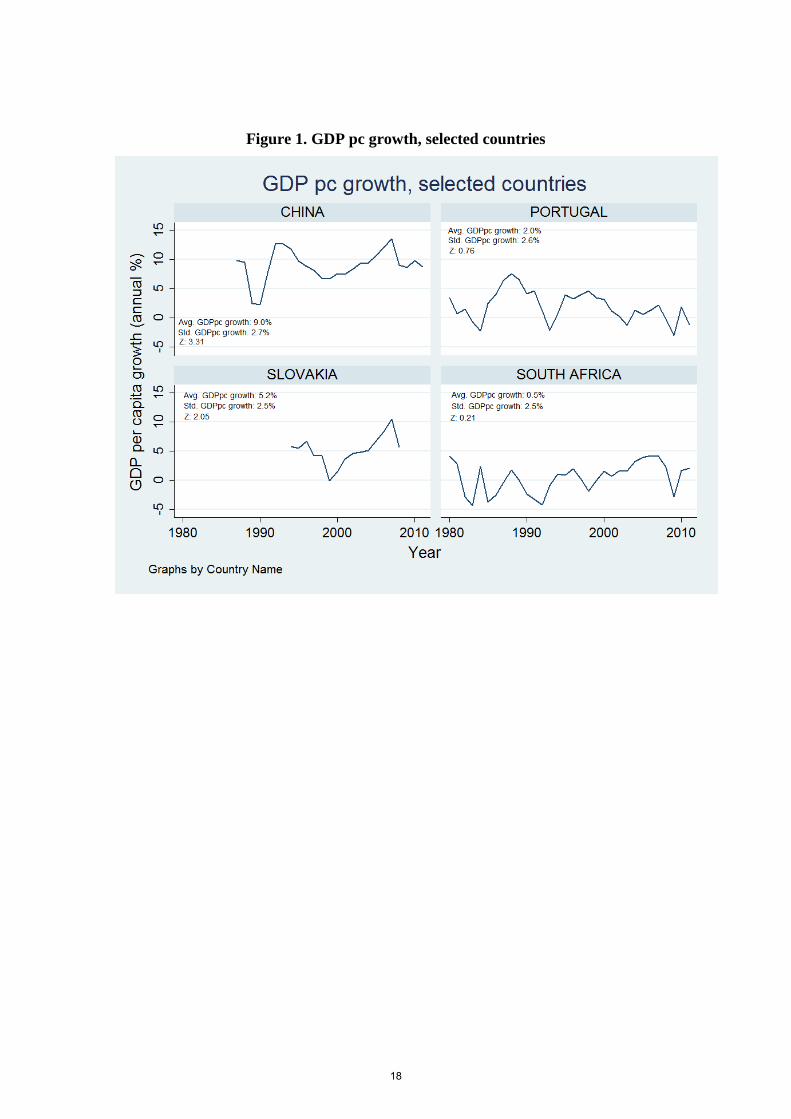
Figure 1. GDP pc growth, selected countries

18

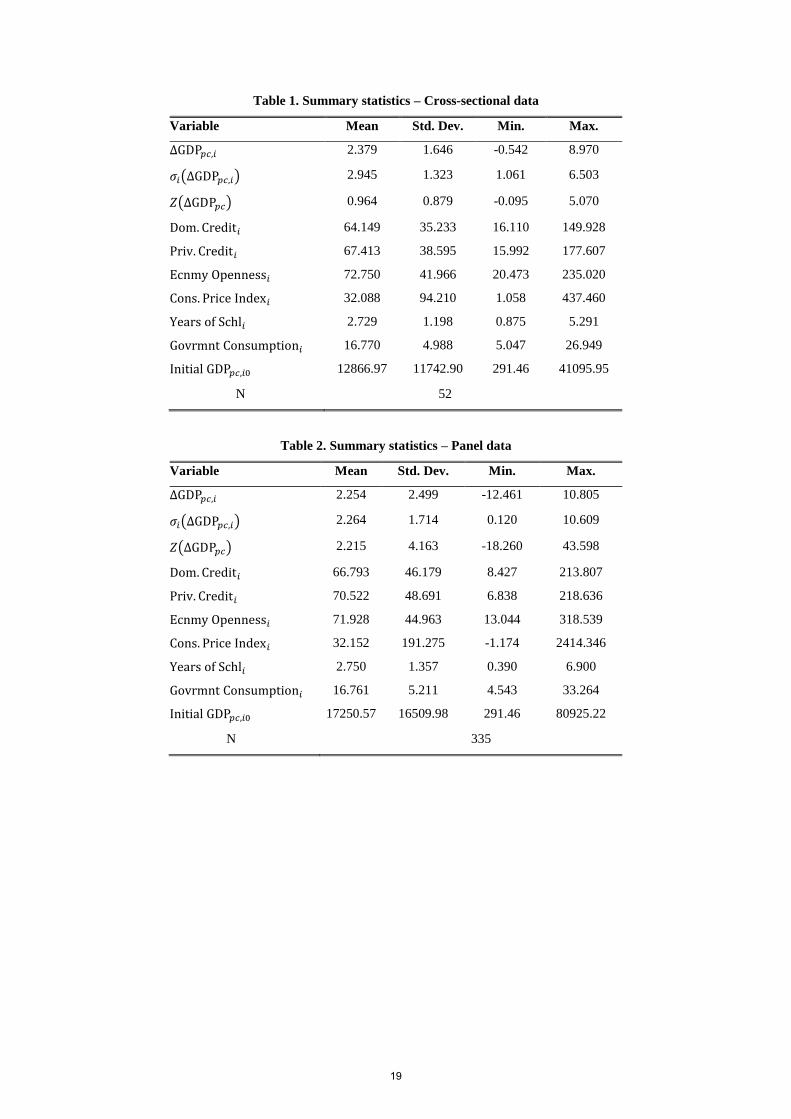
Table 1. Summary statistics – Cross-sectional data

Variable Mean Std. Dev. Min. Max.

ΔGDP𝑝𝑐,𝑖 2.379 1.646 -0.542 8.970

𝜎𝑖(ΔGDP𝑝𝑐,𝑖) 2.945 1.323 1.061 6.503

𝑍(ΔGDP𝑝𝑐) 0.964 0.879 -0.095 5.070

Dom. Credit𝑖 64.149 35.233 16.110 149.928

Priv. Credit𝑖 67.413 38.595 15.992 177.607

Ecnmy Openness𝑖 72.750 41.966 20.473 235.020

Cons. Price Index𝑖 32.088 94.210 1.058 437.460

Years of Schl𝑖 2.729 1.198 0.875 5.291

Govrmnt Consumption𝑖 16.770 4.988 5.047 26.949

Initial GDP𝑝𝑐,𝑖0 12866.97 11742.90 291.46 41095.95

N 52

Table 2. Summary statistics – Panel data

Variable Mean Std. Dev. Min. Max.

ΔGDP𝑝𝑐,𝑖 2.254 2.499 -12.461 10.805

𝜎𝑖(ΔGDP𝑝𝑐,𝑖) 2.264 1.714 0.120 10.609

𝑍(ΔGDP𝑝𝑐) 2.215 4.163 -18.260 43.598

Dom. Credit𝑖 66.793 46.179 8.427 213.807

Priv. Credit𝑖 70.522 48.691 6.838 218.636

Ecnmy Openness𝑖 71.928 44.963 13.044 318.539

Cons. Price Index𝑖 32.152 191.275 -1.174 2414.346

Years of Schl𝑖 2.750 1.357 0.390 6.900

Govrmnt Consumption𝑖 16.761 5.211 4.543 33.264

Initial GDP𝑝𝑐,𝑖0 17250.57 16509.98 291.46 80925.22

N 335

19

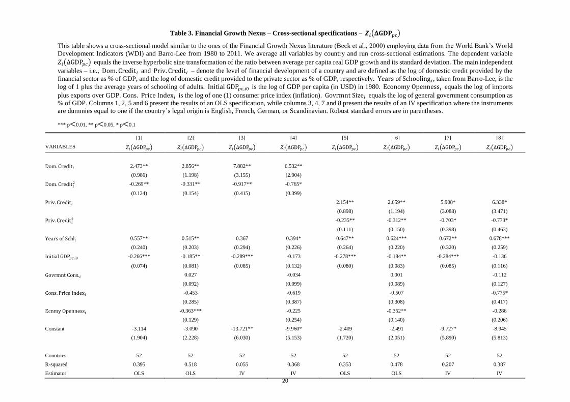
Table 3. Financial Growth Nexus – Cross-sectional specifications – 𝒁𝒊(𝚫𝐆𝐃𝐏𝒑𝒄)

This table shows a cross-sectional model similar to the ones of the Financial Growth Nexus literature (Beck et al., 2000) employing data from the World Bank’s World

Development Indicators (WDI) and Barro-Lee from 1980 to 2011. We average all variables by country and run cross-sectional estimations. The dependent variable

𝑍𝑖(ΔGDP𝑝𝑐) equals the inverse hyperbolic sine transformation of the ratio between average per capita real GDP growth and its standard deviation. The main independent

variables – i.e., Dom. Credit𝑖 and Priv. Credit𝑖 – denote the level of financial development of a country and are defined as the log of domestic credit provided by the

financial sector as % of GDP, and the log of domestic credit provided to the private sector as % of GDP, respectively. Years of Schooling𝑖, taken from Barro-Lee, is the

log of 1 plus the average years of schooling of adults. Initial GDP𝑝𝑐,𝑖0 is the log of GDP per capita (in USD) in 1980. Economy Openness𝑖 equals the log of imports

plus exports over GDP. Cons. Price Index𝑖 is the log of one (1) consumer price index (inflation). Govrmnt Size𝑖 equals the log of general government consumption as

% of GDP. Columns 1, 2, 5 and 6 present the results of an OLS specification, while columns 3, 4, 7 and 8 present the results of an IV specification where the instruments

are dummies equal to one if the country’s legal origin is English, French, German, or Scandinavian. Robust standard errors are in parentheses.

*** p<0.01, ** p<0.05, * p<0.1

[1] [2] [3] [4] [5] [6] [7] [8]

VARIABLES 𝑍𝑖(ΔGDP𝑝𝑐) 𝑍𝑖(ΔGDP𝑝𝑐) 𝑍𝑖(ΔGDP𝑝𝑐) 𝑍𝑖(ΔGDP𝑝𝑐) 𝑍𝑖(ΔGDP𝑝𝑐) 𝑍𝑖(ΔGDP𝑝𝑐) 𝑍𝑖(ΔGDP𝑝𝑐) 𝑍𝑖(ΔGDP𝑝𝑐)

Dom. Credit𝑖 2.473** 2.856** 7.882** 6.532**

(0.986) (1.198) (3.155) (2.904)

Dom. Credit𝑖2 -0.269** -0.331** -0.917** -0.765*

(0.124) (0.154) (0.415) (0.399)

Priv. Credit𝑖 2.154** 2.659** 5.908* 6.338*

(0.898) (1.194) (3.088) (3.471)

Priv. Credit𝑖2 -0.235** -0.312** -0.703* -0.773*

(0.111) (0.150) (0.398) (0.463)

Years of Schl𝑖 0.557** 0.515** 0.367 0.394* 0.647** 0.624*** 0.672** 0.678***

(0.240) (0.203) (0.294) (0.226) (0.264) (0.220) (0.320) (0.259)

Initial GDP𝑝𝑐,𝑖0 -0.266*** -0.185** -0.289*** -0.173 -0.278*** -0.184** -0.284*** -0.136

(0.074) (0.081) (0.085) (0.132) (0.080) (0.083) (0.085) (0.116)

Govrmnt Cons.𝑖 0.027 -0.034 0.001 -0.112

(0.092) (0.099) (0.089) (0.127)

Cons. Price Index𝑖 -0.453 -0.619 -0.507 -0.775*

(0.285) (0.387) (0.308) (0.417)

Ecnmy Openness𝑖 -0.363*** -0.225 -0.352** -0.286

(0.129) (0.254) (0.140) (0.206)

Constant -3.114 -3.090 -13.721** -9.960* -2.409 -2.491 -9.727* -8.945

(1.904) (2.228) (6.030) (5.153) (1.720) (2.051) (5.890) (5.813)

Countries 52 52 52 52 52 52 52 52

R-squared 0.395 0.518 0.055 0.368 0.353 0.478 0.207 0.387

Estimator OLS OLS IV IV OLS OLS IV IV

20

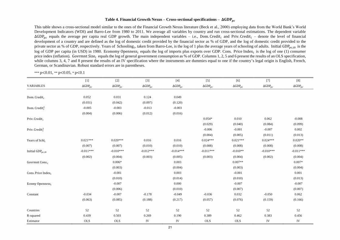
Table 4. Financial Growth Nexus – Cross-sectional specifications – 𝚫𝐆𝐃𝐏𝒑𝒄



ΔGDP𝑝𝑐 equals the average per capita real GDP growth. The main independent variables – i.e., Dom. Credit𝑖 and Priv. Credit𝑖 – denote the level of financial

development of a country and are defined as the log of domestic credit provided by the financial sector as % of GDP, and the log of domestic credit provided to the

private sector as % of GDP, respectively. Years of Schooling𝑖, taken from Barro-Lee, is the log of 1 plus the average years of schooling of adults. Initial GDP𝑝𝑐,𝑖0 is the

log of GDP per capita (in USD) in 1980. Economy Openness𝑖 equals the log of imports plus exports over GDP. Cons. Price Index𝑖 is the log of one (1) consumer

price index (inflation). Govrmnt Size𝑖 equals the log of general government consumption as % of GDP. Columns 1, 2, 5 and 6 present the results of an OLS specification,

while columns 3, 4, 7 and 8 present the results of an IV specification where the instruments are dummies equal to one if the country’s legal origin is English, French,

German, or Scandinavian. Robust standard errors are in parentheses.

*** p<0.01, ** p<0.05, * p<0.1

[1] [2] [3] [4] [5] [6] [7] [8]

VARIABLES ΔGDP𝑝𝑐 ΔGDP𝑝𝑐 ΔGDP𝑝𝑐 ΔGDP𝑝𝑐 ΔGDP𝑝𝑐 ΔGDP𝑝𝑐 ΔGDP𝑝𝑐 ΔGDP𝑝𝑐

Dom. Credit𝑖 0.052 0.031 0.124 0.049

(0.031) (0.042) (0.097) (0.120)

Dom. Credit𝑖2 -0.005 -0.003 -0.013 -0.003

(0.004) (0.006) (0.012) (0.016)

Priv. Credit𝑖 0.054* 0.010 0.062 -0.008

(0.029) (0.040) (0.084) (0.099)

Priv. Credit𝑖2 -0.006 -0.001 -0.007 0.002

(0.004) (0.005) (0.011) (0.013)

Years of Schl𝑖 0.021*** 0.020*** 0.016 0.016 0.024*** 0.021*** 0.024*** 0.020**

(0.007) (0.007) (0.010) (0.010) (0.008) (0.008) (0.008) (0.008)

Initial GDP𝑝𝑐,𝑖0 -0.011*** -0.010*** -0.012*** -0.014*** -0.011*** -0.010** -0.010*** -0.011***

(0.002) (0.004) (0.003) (0.005) (0.003) (0.004) (0.002) (0.004)

Govrmnt Cons.𝑖 0.006* 0.003 0.007** 0.007*

(0.003) (0.004) (0.003) (0.004)

Cons. Price Index𝑖 -0.001 0.003 -0.001 0.001

(0.010) (0.014) (0.010) (0.013)

Ecnmy Openness𝑖 -0.007 0.000 -0.007 -0.007

(0.006) (0.010) (0.007) (0.007)

Constant -0.034 -0.007 -0.178 -0.049 -0.036 0.032 -0.050 0.062

(0.063) (0.085) (0.188) (0.217) (0.057) (0.076) (0.159) (0.166)

Countries 52 52 52 52 52 52 52 52

R-squared 0.439 0.503 0.269 0.190 0.389 0.462 0.383 0.456


21

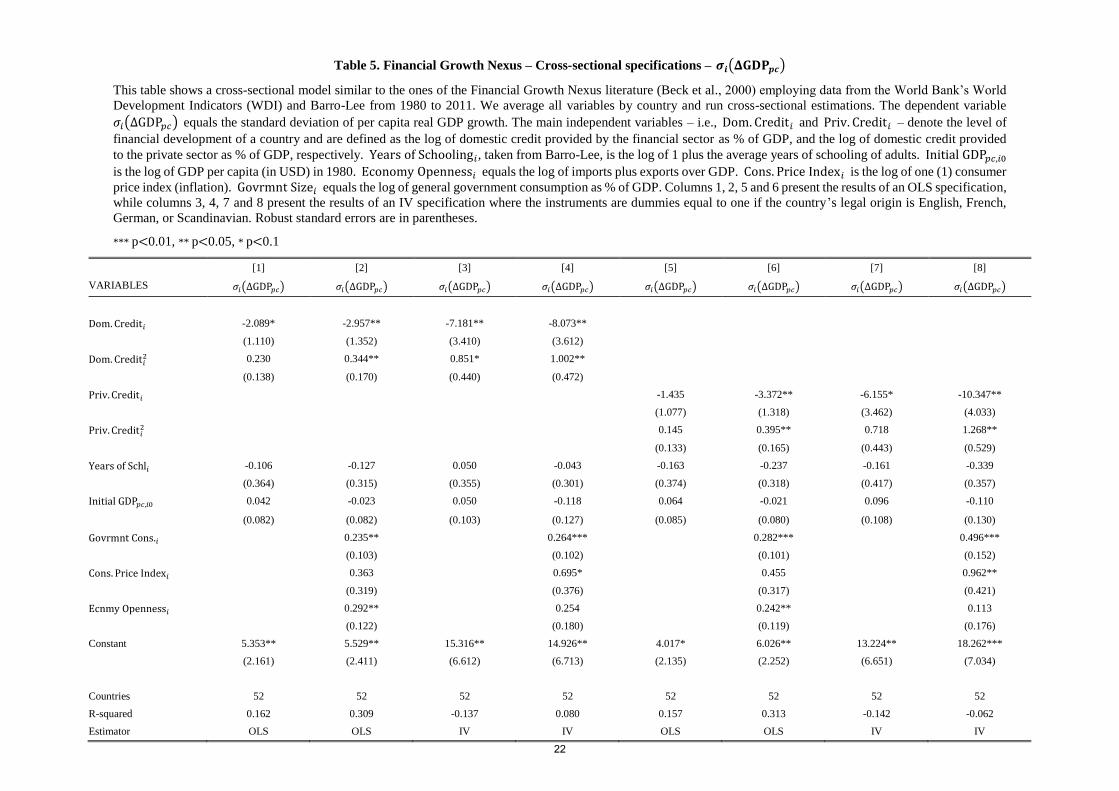
Table 5. Financial Growth Nexus – Cross-sectional specifications – 𝝈𝒊(𝚫𝐆𝐃𝐏𝒑𝒄)



𝜎𝑖(ΔGDP𝑝𝑐) equals the standard deviation of per capita real GDP growth. The main independent variables – i.e., Dom. Credit𝑖 and Priv. Credit𝑖 – denote the level of

financial development of a country and are defined as the log of domestic credit provided by the financial sector as % of GDP, and the log of domestic credit provided

to the private sector as % of GDP, respectively. Years of Schooling𝑖, taken from Barro-Lee, is the log of 1 plus the average years of schooling of adults. Initial GDP𝑝𝑐,𝑖0

is the log of GDP per capita (in USD) in 1980. Economy Openness𝑖 equals the log of imports plus exports over GDP. Cons. Price Index𝑖 is the log of one (1) consumer

price index (inflation). Govrmnt Size𝑖 equals the log of general government consumption as % of GDP. Columns 1, 2, 5 and 6 present the results of an OLS specification,

while columns 3, 4, 7 and 8 present the results of an IV specification where the instruments are dummies equal to one if the country’s legal origin is English, French,

German, or Scandinavian. Robust standard errors are in parentheses.

*** p<0.01, ** p<0.05, * p<0.1

[1] [2] [3] [4] [5] [6] [7] [8]

VARIABLES 𝜎𝑖(ΔGDP𝑝𝑐) 𝜎𝑖(ΔGDP𝑝𝑐) 𝜎𝑖(ΔGDP𝑝𝑐) 𝜎𝑖(ΔGDP𝑝𝑐) 𝜎𝑖(ΔGDP𝑝𝑐) 𝜎𝑖(ΔGDP𝑝𝑐) 𝜎𝑖(ΔGDP𝑝𝑐) 𝜎𝑖(ΔGDP𝑝𝑐)

Dom. Credit𝑖 -2.089* -2.957** -7.181** -8.073**

(1.110) (1.352) (3.410) (3.612)

Dom. Credit𝑖2 0.230 0.344** 0.851* 1.002**

(0.138) (0.170) (0.440) (0.472)

Priv. Credit𝑖 -1.435 -3.372** -6.155* -10.347**

(1.077) (1.318) (3.462) (4.033)

Priv. Credit𝑖2 0.145 0.395** 0.718 1.268**

(0.133) (0.165) (0.443) (0.529)

Years of Schl𝑖 -0.106 -0.127 0.050 -0.043 -0.163 -0.237 -0.161 -0.339

(0.364) (0.315) (0.355) (0.301) (0.374) (0.318) (0.417) (0.357)

Initial GDP𝑝𝑐,𝑖0 0.042 -0.023 0.050 -0.118 0.064 -0.021 0.096 -0.110

(0.082) (0.082) (0.103) (0.127) (0.085) (0.080) (0.108) (0.130)

Govrmnt Cons.𝑖 0.235** 0.264*** 0.282*** 0.496***

(0.103) (0.102) (0.101) (0.152)

Cons. Price Index𝑖 0.363 0.695* 0.455 0.962**

(0.319) (0.376) (0.317) (0.421)

Ecnmy Openness𝑖 0.292** 0.254 0.242** 0.113

(0.122) (0.180) (0.119) (0.176)

Constant 5.353** 5.529** 15.316** 14.926** 4.017* 6.026** 13.224** 18.262***

(2.161) (2.411) (6.612) (6.713) (2.135) (2.252) (6.651) (7.034)

Countries 52 52 52 52 52 52 52 52

R-squared 0.162 0.309 -0.137 0.080 0.157 0.313 -0.142 -0.062


22

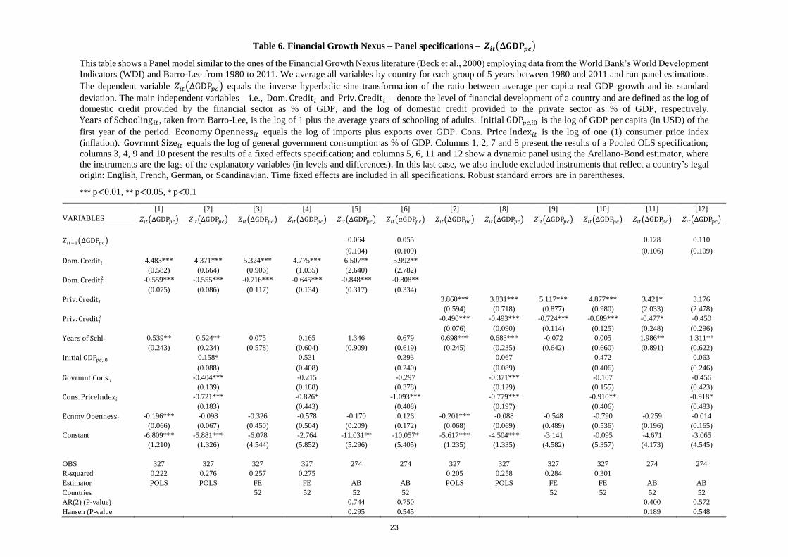
Table 6. Financial Growth Nexus – Panel specifications – 𝒁𝒊𝒕(𝚫𝐆𝐃𝐏𝒑𝒄)

This table shows a Panel model similar to the ones of the Financial Growth Nexus literature (Beck et al., 2000) employing data from the World Bank’s World Development

Indicators (WDI) and Barro-Lee from 1980 to 2011. We average all variables by country for each group of 5 years between 1980 and 2011 and run panel estimations.

The dependent variable 𝑍𝑖𝑡(ΔGDP𝑝𝑐) equals the inverse hyperbolic sine transformation of the ratio between average per capita real GDP growth and its standard

deviation. The main independent variables – i.e., Dom. Credit𝑖 and Priv. Credit𝑖 – denote the level of financial development of a country and are defined as the log of

domestic credit provided by the financial sector as % of GDP, and the log of domestic credit provided to the private sector as % of GDP, respectively.

Years of Schooling𝑖𝑡 , taken from Barro-Lee, is the log of 1 plus the average years of schooling of adults. Initial GDP𝑝𝑐,𝑖0 is the log of GDP per capita (in USD) of the

first year of the period. Economy Openness𝑖𝑡 equals the log of imports plus exports over GDP. Cons. Price Index𝑖𝑡 is the log of one (1) consumer price index

(inflation). Govrmnt Size𝑖𝑡 equals the log of general government consumption as % of GDP. Columns 1, 2, 7 and 8 present the results of a Pooled OLS specification;

columns 3, 4, 9 and 10 present the results of a fixed effects specification; and columns 5, 6, 11 and 12 show a dynamic panel using the Arellano-Bond estimator, where

the instruments are the lags of the explanatory variables (in levels and differences). In this last case, we also include excluded instruments that reflect a country’s legal

origin: English, French, German, or Scandinavian. Time fixed effects are included in all specifications. Robust standard errors are in parentheses.

*** p<0.01, ** p<0.05, * p<0.1

[1] [2] [3] [4] [5] [6] [7] [8] [9] [10] [11] [12]

VARIABLES 𝑍𝑖𝑡(ΔGDP𝑝𝑐) 𝑍𝑖𝑡(ΔGDP𝑝𝑐) 𝑍𝑖𝑡(ΔGDP𝑝𝑐) 𝑍𝑖𝑡(ΔGDP𝑝𝑐) 𝑍𝑖𝑡(ΔGDP𝑝𝑐) 𝑍𝑖𝑡(𝑎GDP𝑝𝑐) 𝑍𝑖𝑡(ΔGDP𝑝𝑐) 𝑍𝑖𝑡(ΔGDP𝑝𝑐) 𝑍𝑖𝑡(ΔGDP𝑝𝑐) 𝑍𝑖𝑡(ΔGDP𝑝𝑐) 𝑍𝑖𝑡(ΔGDP𝑝𝑐) 𝑍𝑖𝑡(ΔGDP𝑝𝑐)

𝑍𝑖𝑡−1(ΔGDP𝑝𝑐) 0.064 0.055 0.128 0.110

(0.104) (0.109) (0.106) (0.109)

Dom. Credit𝑖 4.483*** 4.371*** 5.324*** 4.775*** 6.507** 5.992**

(0.582) (0.664) (0.906) (1.035) (2.640) (2.782)

Dom. Credit𝑖2 -0.559*** -0.555*** -0.716*** -0.645*** -0.848*** -0.808**

(0.075) (0.086) (0.117) (0.134) (0.317) (0.334)

Priv. Credit𝑖 3.860*** 3.831*** 5.117*** 4.877*** 3.421* 3.176

(0.594) (0.718) (0.877) (0.980) (2.033) (2.478)

Priv. Credit𝑖2 -0.490*** -0.493*** -0.724*** -0.689*** -0.477* -0.450

(0.076) (0.090) (0.114) (0.125) (0.248) (0.296)

Years of Schl𝑖 0.539** 0.524** 0.075 0.165 1.346 0.679 0.698*** 0.683*** -0.072 0.005 1.986** 1.311**

(0.243) (0.234) (0.578) (0.604) (0.909) (0.619) (0.245) (0.235) (0.642) (0.660) (0.891) (0.622)

Initial GDP𝑝𝑐,𝑖0 0.158* 0.531 0.393 0.067 0.472 0.063

(0.088) (0.408) (0.240) (0.089) (0.406) (0.246)

Govrmnt Cons.𝑖 -0.404*** -0.215 -0.297 -0.371*** -0.107 -0.456

(0.139) (0.188) (0.378) (0.129) (0.155) (0.423)

Cons. PriceIndex𝑖 -0.721*** -0.826* -1.093*** -0.779*** -0.910** -0.918*

(0.183) (0.443) (0.408) (0.197) (0.406) (0.483)

Ecnmy Openness𝑖 -0.196*** -0.098 -0.326 -0.578 -0.170 0.126 -0.201*** -0.088 -0.548 -0.790 -0.259 -0.014

(0.066) (0.067) (0.450) (0.504) (0.209) (0.172) (0.068) (0.069) (0.489) (0.536) (0.196) (0.165)

Constant -6.809*** -5.881*** -6.078 -2.764 -11.031** -10.057* -5.617*** -4.504*** -3.141 -0.095 -4.671 -3.065

(1.210) (1.326) (4.544) (5.852) (5.296) (5.405) (1.235) (1.335) (4.582) (5.357) (4.173) (4.545)

OBS 327 327 327 327 274 274 327 327 327 327 274 274

R-squared 0.222 0.276 0.257 0.275 0.205 0.258 0.284 0.301

Estimator POLS POLS FE FE AB AB POLS POLS FE FE AB AB

Countries 52 52 52 52 52 52 52 52

AR(2) (P-value) 0.744 0.750 0.400 0.572

Hansen (P-value 0.295 0.545 0.189 0.548

23

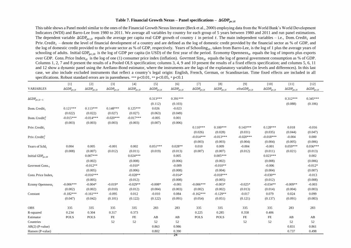
Table 7. Financial Growth Nexus – Panel specifications – 𝚫𝐆𝐃𝐏𝒑𝒄,𝒊𝒕



The dependent variable ΔGDP𝑝𝑐,𝑖𝑡 equals the average per capita real GDP growth of country 𝑖 in period 𝑡. The main independent variables – i.e., Dom. Credit𝑖 and

Priv. Credit𝑖 – denote the level of financial development of a country and are defined as the log of domestic credit provided by the financial sector as % of GDP, and

the log of domestic credit provided to the private sector as % of GDP, respectively. Years of Schooling𝑖𝑡 , taken from Barro-Lee, is the log of 1 plus the average years of

schooling of adults. Initial GDP𝑝𝑐,𝑖0 is the log of GDP per capita (in USD) of the first year of the period. Economy Openness𝑖𝑡 equals the log of imports plus exports

over GDP. Cons. Price Index𝑖𝑡 is the log of one (1) consumer price index (inflation). Govrmnt Size𝑖𝑡 equals the log of general government consumption as % of GDP.

Columns 1, 2, 7 and 8 present the results of a Pooled OLS specification; columns 3, 4, 9 and 10 present the results of a fixed effects specification; and columns 5, 6, 11

and 12 show a dynamic panel using the Arellano-Bond estimator, where the instruments are the lags of the explanatory variables (in levels and differences). In this last

case, we also include excluded instruments that reflect a country’s legal origin: English, French, German, or Scandinavian. Time fixed effects are included in all

specifications. Robust standard errors are in parentheses. *** p<0.01, ** p<0.05, * p<0.1

[1] [2] [3] [4] [5] [6] [7] [8] [9] [10] [11] [12]

VARIABLES ΔGDP𝑝𝑐,𝑖𝑡 ΔGDP𝑝𝑐,𝑖𝑡 ΔGDP𝑝𝑐,𝑖𝑡 ΔGDP𝑝𝑐,𝑖𝑡 ΔGDP𝑝𝑐,𝑖𝑡 ΔGDP𝑝𝑐,𝑖𝑡 ΔGDP𝑝𝑐,𝑖𝑡 ΔGDP𝑝𝑐,𝑖𝑡 𝑒𝑙𝑡𝑎GDP𝑝𝑐,𝑖𝑡 ΔGDP𝑝𝑐,𝑖𝑡 ΔGDP𝑝𝑐,𝑖𝑡 ΔGDP𝑝𝑐,𝑖𝑡

ΔGDP𝑝𝑐,𝑖𝑡−1 0.313*** 0.391*** 0.312*** 0.345***

(0.112) (0.103) (0.088) (0.106)

Dom. Credit𝑖 0.121*** 0.113*** 0.148*** 0.125*** 0.026 -0.023

(0.022) (0.022) (0.027) (0.027) (0.063) (0.049)

Dom. Credit𝑖2 -0.015*** -0.014*** -0.020*** -0.017*** -0.005 0.001

(0.003) (0.003) (0.003) (0.003) (0.007) (0.006)

Priv. Credit𝑖 0.110*** 0.100*** 0.143*** 0.128*** 0.018 -0.016

(0.026) (0.028) (0.031) (0.035) (0.044) (0.047)

Priv. Credit𝑖2 -0.014*** -0.013*** -0.020*** -0.018*** -0.004 0.000

(0.003) (0.003) (0.004) (0.004) (0.005) (0.006)

Years of Schl𝑖 0.004 0.005 -0.001 0.002 0.051*** 0.028** 0.010 0.009 -0.004 -0.001 0.059*** 0.036***

(0.008) (0.007) (0.012) (0.011) (0.019) (0.013) (0.007) (0.007) (0.012) (0.011) (0.021) (0.013)

Initial GDP𝑝𝑐,𝑖0 0.007*** 0.024*** 0.005 0.005*** 0.023*** 0.002

(0.002) (0.008) (0.006) (0.002) (0.008) (0.006)

Govrmnt Cons.𝑖 -0.012** -0.010* -0.009 -0.010** -0.006 -0.012*

(0.005) (0.006) (0.008) (0.004) (0.004) (0.007)

Cons. Price Index𝑖 -0.016*** -0.028** -0.014* -0.018*** -0.030** -0.013

(0.005) (0.012) (0.008) (0.005) (0.012) (0.008)

Ecnmy Openness𝑖 -0.006*** -0.004* -0.019* -0.029** -0.008* -0.001 -0.006*** -0.003* -0.025* -0.034** -0.009** -0.003

(0.002) (0.002) (0.010) (0.012) (0.004) (0.003) (0.002) (0.002) (0.013) (0.014) (0.004) (0.003)

Constant -0.182*** -0.161*** -0.095 0.012 -0.010 0.084 -0.162*** -0.129** -0.017 0.079 0.024 0.099

(0.047) (0.042) (0.101) (0.122) (0.122) (0.091) (0.054) (0.051) (0.121) (0.137) (0.091) (0.083)

OBS 335 335 335 335 283 283 335 335 335 335 283 283

R-squared 0.234 0.304 0.317 0.373 0.225 0.285 0.358 0.406


Countries 52 52 52 52 52 52 52 52

AR(2) (P-value) 0.863 0.986 0.831 0.861

Hansen (P-value) 0.802 0.390 0.737 0.498 24

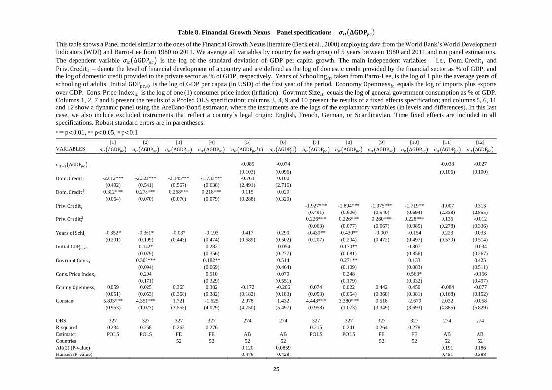
Table 8. Financial Growth Nexus – Panel specifications – 𝝈𝒊𝒕(𝚫𝐆𝐃𝐏𝒑𝒄)



The dependent variable 𝜎𝑖𝑡(ΔGDP𝑝𝑐) is the log of the standard deviation of GDP per capita growth. The main independent variables – i.e., Dom. Credit𝑖 and

Priv. Credit𝑖 – denote the level of financial development of a country and are defined as the log of domestic credit provided by the financial sector as % of GDP, and

the log of domestic credit provided to the private sector as % of GDP, respectively. Years of Schooling𝑖𝑡 , taken from Barro-Lee, is the log of 1 plus the average years of

schooling of adults. Initial GDP𝑝𝑐,𝑖0 is the log of GDP per capita (in USD) of the first year of the period. Economy Openness𝑖𝑡 equals the log of imports plus exports

over GDP. Cons. Price Index𝑖𝑡 is the log of one (1) consumer price index (inflation). Govrmnt Size𝑖𝑡 equals the log of general government consumption as % of GDP.

Columns 1, 2, 7 and 8 present the results of a Pooled OLS specification; columns 3, 4, 9 and 10 present the results of a fixed effects specification; and columns 5, 6, 11

and 12 show a dynamic panel using the Arellano-Bond estimator, where the instruments are the lags of the explanatory variables (in levels and differences). In this last

case, we also include excluded instruments that reflect a country’s legal origin: English, French, German, or Scandinavian. Time fixed effects are included in all

specifications. Robust standard errors are in parentheses.

*** p<0.01, ** p<0.05, * p<0.1

[1] [2] [3] [4] [5] [6] [7] [8] [9] [10] [11] [12]

VARIABLES 𝜎𝑖𝑡(ΔGDP𝑝𝑐) 𝜎𝑖𝑡(ΔGDP𝑝𝑐) 𝜎𝑖𝑡(ΔGDP𝑝𝑐) 𝜎𝑖𝑡(ΔGDP𝑝𝑐) 𝜎𝑖𝑡(ΔGDP𝑝𝑐ℎ𝑡) 𝜎𝑖𝑡(ΔGDP𝑝𝑐) 𝜎𝑖𝑡(ΔGDP𝑝𝑐) 𝜎𝑖𝑡(ΔGDP𝑝𝑐) 𝜎𝑖𝑡(ΔGDP𝑝𝑐) 𝜎𝑖𝑡(ΔGDP𝑝𝑐) 𝜎𝑖𝑡(ΔGDP𝑝𝑐) 𝜎𝑖𝑡(ΔGDP𝑝𝑐)

𝜎𝑖𝑡−1(ΔGDP𝑝𝑐) -0.085 -0.074 -0.038 -0.027

(0.103) (0.096) (0.106) (0.100)

Dom. Credit𝑖 -2.612*** -2.322*** -2.145*** -1.733*** -0.763 0.100

(0.492) (0.541) (0.567) (0.638) (2.491) (2.716)

Dom. Credit𝑖2 0.312*** 0.278*** 0.268*** 0.218*** 0.115 0.020

(0.064) (0.070) (0.070) (0.079) (0.288) (0.320)

Priv. Credit𝑖 -1.927*** -1.894*** -1.975*** -1.719** -1.007 0.313

(0.491) (0.606) (0.540) (0.694) (2.338) (2.855)

Priv. Credit𝑖2 0.226*** 0.226*** 0.260*** 0.228*** 0.136 -0.012

(0.063) (0.077) (0.067) (0.085) (0.278) (0.336)

Years of Schl𝑖 -0.352* -0.361* -0.037 -0.193 0.417 0.290 -0.430** -0.430** -0.007 -0.154 0.223 0.033

(0.201) (0.199) (0.443) (0.474) (0.589) (0.502) (0.207) (0.204) (0.472) (0.497) (0.570) (0.514)

Initial GDP𝑝𝑐,𝑖0 0.142* 0.282 -0.054 0.170** 0.307 -0.034

(0.079) (0.356) (0.277) (0.081) (0.356) (0.267)

Govrmnt Cons.𝑖 0.308*** 0.182** 0.514 0.271** 0.133 0.425

(0.094) (0.069) (0.464) (0.109) (0.083) (0.511)

Cons. Price Index𝑖 0.204 0.510 0.070 0.248 0.563* -0.156

(0.171) (0.329) (0.551) (0.179) (0.332) (0.497)

Ecnmy Openness𝑖 0.059 0.025 0.365 0.382 -0.172 -0.206 0.074 0.022 0.442 0.450 -0.084 -0.077

(0.051) (0.053) (0.368) (0.382) (0.182) (0.183) (0.053) (0.054) (0.368) (0.381) (0.168) (0.152)

Constant 5.803*** 4.351*** 1.721 -1.625 2.978 1.432 4.443*** 3.380*** 0.518 -2.679 2.032 -0.058

(0.953) (1.027) (3.555) (4.029) (4.750) (5.497) (0.958) (1.073) (3.349) (3.693) (4.885) (5.829)

OBS 327 327 327 327 274 274 327 327 327 327 274 274

R-squared 0.234 0.258 0.263 0.276 0.215 0.241 0.264 0.278


Countries 52 52 52 52 52 52 52 52

AR(2) (P-value) 0.120 0.0859 0.191 0.186

Hansen (P-value) 0.476 0.428 0.451 0.388

25

Appendix A. Data Sources

Variable Variable definition Source

ΔGDP𝑝𝑐 GDP per capita growth World Bank WDI

𝜎𝑖(ΔGDP𝑝𝑐) Log of the standard deviation of GDP per capita growth Own calculation

𝑍(ΔGDP𝑝𝑐) The inverse hyperbolic sine transformation of the

average GDP per capita growth divided by the standard

deviation of GDP per capita growth

Own calculation

Dom. Credit The log of domestic credit to the private sector by banks

(% of GDP)

World Bank WDI

Priv. Credit The log of private credit by deposit money banks and

other financial institutions to GDP (% of GDP)

World Bank GFDD

Ecnmy. Openness Log of the sum of imports and exports of goods and

services (% of GDP)

World Bank WDI

Cons. Price Index Log of 1 plus consumer price index inflation World Bank WDI

Years of Schl Log of 1 plus the average years of secondary schooling

in the total population (25 years and over)

Barro-Lee

Govrmnt. Consumption Log of general government final consumption

expenditure (% of GDP)

World Bank WDI

Initial GDP𝑝𝑐,0 Log of GDP per capita from the first year of the period

(2005 prices)

World Bank WDI

26

References

Aghion, Philippe, Peter Howitt, and David Mayer-Foulkes (2005), “The effect of

financial development on convergence: Theory and evidence.” The Quarterly Journal

of Economics, 120, 173–222.

Arcand, Jean Louis, Enrico Berkes, and Ugo Panizza (2015), “Too much finance?”

Journal of Economic Growth, 20, 105–148.

Bagehot, Walter (1873), Lombard Street: A description of the money market, 3 edition.

Henry S. King & Co., London.

Beck, Thorsten, Hans Degryse, and Christiane Kneer (2014), “Is more finance better?

Disentangling intermediation and size effects of financial systems.” Journal of

Financial Stability, 10, 50 – 64.

Beck, Thorsten, Ross Levine, and Norman Loayza (2000), “Finance and the sources of

growth.” Journal of Financial Economics, 58, 261 – 300.

Beck, Thorsten, Mattias Lundberg, and Giovanni Majnoni (2006), “Financial

intermediary development and growth volatility: Do intermediaries dampen or

magnify shocks?” Journal of International Money and Finance, 25, 1146 – 1167.

Cecchetti, Stephen G and Enisse Kharroubi (2012), “Reassessing the impact of finance

on growth.” BIS Working Papers, 381.

Easterly, William, Roumeen Islam, and Joseph E. Stiglitz (2001), Annual World Bank

Conference on Development Economics 2000, chapter Shaken and Stirred: Explaining

Growth Volatility, 191–211. The World Bank.

Goldsmith, Raymond (1969), Financial structure and economic development. Yale

University Press, New Haven.

Gurley, John G. and E. S. Shaw (1955), “Financial aspects of economic development.”

The American Economic Review, 45, 515–538.

Kaminsky, Graciela L. and Carmen M. Reinhart (1999), “The twin crises: The causes of

banking and balance-of-payments problems.” American Economic Review, 89, 473–

500.

King, Robert G. and Ross Levine (1993), “Finance and growth: Schumpeter might be

right.” The Quarterly Journal of Economics, 108, 717–737.

LaPorta, Rafael, Florencio Lopez de Silanes, Andrei Shleifer, and Robert W. Vishny

(1998), “Law and finance.” Journal of Political Economy, 106, 1113–1155.

Law, Siong Hook and Nirvikar Singh (2014), “Does too much finance harm economic

growth?” Journal of Banking & Finance, 41, 36 – 44.

Levine, Ross (2005), “Finance and growth: Theory and evidence.” In Philippe Aghion

and Steven N. Durlauf, (Eds.), Part A of Handbook of Economic Growth volume 1,

Elsevier, 865 – 934.

Levine, Ross, Norman Loayza, and Thorsten Beck (2000), “Financial intermediation and

growth: Causality and causes.” Journal of Monetary Economics, 46, 31 – 77.

Levine, Ross and Sara Zervos (1998), “Stock markets, banks, and economic growth.” The

American Economic Review, 88, pp. 537–558.

27

Loayza, Norman V and Romain Rancire (2006), “Financial development, financial

fragility, and growth.” Journal of Money, Credit, and Banking, 38, 1051–1076.

Mallick, Debdulal (2014), “Financial development, shocks, and growth volatility.”

Macroeconomic Dynamics, 18, 651–688.

Rioja, Felix and Neven Valev (2004), “Does one size fit all?: a reexamination of the

finance and growth relationship.” Journal of Development Economics, 74, 429 – 447.

Roodman, D. (2009), “How to do xtabond2: An introduction to difference and system

gmm in stata.” Stata Journal, 9, 86–136(51).

Sahay, Ratna, Martin Cihak, Papa N’Diaye, Adolfo Barajas, Ran Bi, Diana Ayala, Yuan

Gao, Annette Kyobe, Lam Nguyen, Christian Saborowski, Katsiaryna Svirydzenka,

and Seyed Reza Yousefi (2015), “Rethinking financial deepening: Stability and

growth in emerging markets.” IMF Staff Discussion Note, 15/08, Washington.

Schumpeter, Joseph Alois (1934), The theory of economic development. Harvard

University Press, Cambridge, MA.

Seven, Unal and Hakan Yetkiner (2016), “Financial intermediation and economic growth:

Does income matter?” Economic Systems, 40, 39 – 58.

28

Documents

Economic Growth, Volatility and Their Interaction: … melhor desenvolvimento financeiro levaria a alocações mais eficientes, e assim ... but did not yet have the tools to properly