NBER WORKING PAPER SERIES

EARNINGS ADJUSTMENT FRICTIONS:EVIDENCE FROM THE SOCIAL SECURITY EARNINGS TEST

Alexander M. GelberDamon Jones

Daniel W. Sacks

Working Paper 19491http://www.nber.org/papers/w19491

NATIONAL BUREAU OF ECONOMIC RESEARCH1050 Massachusetts Avenue

Cambridge, MA 02138October 2013

We thank Raj Chetty, Jim Cole, Jim Davis, Mark Duggan, Jonathan Fisher, Richard Freeman, JohnFriedman, Bill Gale, Hilary Hoynes, Adam Isen, Henrik Kleven, Emmanuel Saez, and numerous seminarparticipants. We are extremely grateful to David Pattison for generously running the code on the data.We acknowledge financial support from the Wharton Center for Human Resources and the WhartonRisk and Decision Processes Center, from NIH grant #1R03 AG043039-01, from a National ScienceFoundation Graduate Research Fellowship, and from support from the U.S. Social Security Administrationthrough grant #5RRC08098400- 05-00 to the National Bureau of Economic Research (NBER) as partof the SSA Retirement Research Consortium. The findings and conclusions expressed are solely thoseof the authors and do not represent the views of SSA, any agency of the Federal Government, or theNBER. The research uses data from the Census Bureau's Longitudinal Employer Household DynamicsProgram, which was partially supported by the following National Science Foundation Grants: SES-9978093,SES-0339191 and ITR-0427889; National Institute on Aging Grant AG018854; and grants from theAlfred P. Sloan Foundation. All results have been reviewed to ensure that no confidential informationis disclosed. All errors are our own.

At least one co-author has disclosed a financial relationship of potential relevance for this research.Further information is available online at http://www.nber.org/papers/w19491.ack

NBER working papers are circulated for discussion and comment purposes. They have not been peer-reviewed or been subject to the review by the NBER Board of Directors that accompanies officialNBER publications.

© 2013 by Alexander M. Gelber, Damon Jones, and Daniel W. Sacks. All rights reserved. Short sectionsof text, not to exceed two paragraphs, may be quoted without explicit permission provided that fullcredit, including © notice, is given to the source.

Earnings Adjustment Frictions: Evidence from the Social Security Earnings TestAlexander M. Gelber, Damon Jones, and Daniel W. SacksNBER Working Paper No. 19491October 2013JEL No. H20,H31,J14,J26

ABSTRACT

We study frictions in adjusting earnings to changes in the Social Security Annual Earnings Test (AET)using a panel of Social Security Administration microdata on one percent of the U.S. population from1961 to 2006. Individuals continue to "bunch" at the convex kink the AET creates even when theyare no longer subject to the AET, consistent with the existence of earnings adjustment frictions in theU.S. We develop a novel framework for estimating an earnings elasticity and an adjustment cost usinginformation on the amount of bunching at kinks before and after policy changes in earnings incentivesaround the kinks. We apply this method in settings in which individuals face changes in the AET benefitreduction rate, and we estimate in a baseline case that the earnings elasticity with respect to the implicitnet-of-tax share is 0.23, and the fixed cost of adjustment is $152.08.

Alexander M. GelberGoldman School of Public PolicyUniversity of California at Berkeley2607 Hearst AveBerkeley, CA 94720and NBERagelber@berkeley.edu

Damon JonesHarris School of Public PolicyUniversity of Chicago1155 East 60th StreetChicago, IL 60637and NBERdamonjones@uchicago.edu

Daniel W. SacksThe Wharton SchoolUniversity of Pennsylvania3620 Locust WalkPhiladelphia, PA 19104dansacks@wharton.upenn.edu

1 Introduction

In a traditional model of workers’earnings or labor supply choices, individuals optimize their

behavior frictionlessly in response to policies that affect their incentives. However, several

recent papers have suggested that individuals face frictions in adjusting behavior to policy

(Chetty, Looney, and Kroft 2009; Chetty, Friedman, Olsen, and Pistaferri 2011; Chetty,

Guren, Manoli, and Weber 2012; Chetty, Friedman, and Saez 2012; Chetty 2012; Kleven

and Waseem 2013). Costs of adjusting behavior help to govern the welfare cost of taxation

(Chetty et al. 2009), and they also help to explain heterogeneity across contexts in the

observed elasticity of earnings with respect to the net-of-tax rate (Chetty et al. 2011, 2012b;

Chetty 2012).1

This paper develops evidence on the existence, nature and size of frictions in adjusting

earnings in response to policy. The U.S. Social Security Annual Earnings Test (AET) repre-

sents a promising environment for studying these questions. This setting provides a useful

illustration of many issues– such as the development and application of a methodology for

estimating elasticities and adjustment costs simultaneously– that are applicable to studying

earnings responses to policy more broadly. The AET reduces Social Security Old Age and

Survivors Insurance (OASI) claimants’current OASI benefits as a proportion of earnings,

once an individual earns in excess of an exempt amount. For example, for OASI claimants

aged 62-65 in 2013, current OASI benefits are reduced by 50 cents for every extra dollar

earned above $15,120. The AET may lead to very large effective benefit reduction rates

(BRRs) on earnings above the exempt amount, creating a strong incentive for many individ-

uals to “bunch”at the convex kink in the budget constraint located at the exempt amount

(Burtless and Moffi tt 1985; Friedberg, 1998, 2000).2 Reductions in current benefits due to

the AET sometimes lead to increases in later benefits; nonetheless, as we discuss in detail in

Section 2, several factors may explain why individuals’earnings still respond to the AET.

The AET is an appealing context for studying earnings adjustment for at least three

reasons. First, bunching at the AET kink is easily visible on a graph, allowing credible

1The net-of-tax rate is defined as one minus the marginal tax rate (MTR). Literature including Altonji and Paxson (1988)examines hours constraints in the context of labor supply.

2Other papers on the AET include Gruber and Orszag (2003) and Song and Manchester (2007).

1

documentation of behavioral responses.3 Second, the AET represents one of the few known

kinks at which bunching occurs in the U.S.; indeed, our paper represents the first study

to find robust evidence of bunching among the non-self-employed at any kink in the U.S.4

Third, the AET is important to policy-makers in its own right, as it is a significant factor

that affects the earnings of the elderly in the U.S.

We make three main contributions to understanding adjustment frictions. First, we

document that earnings adjustment frictions exist in the U.S., by showing that in some

contexts individuals do not adjust immediately to changes in AET. We focus particularly

on cases in which a kink in the effective tax schedule disappears, either because individuals

reach an age at which they are no longer subject to the AET, or because legislative changes

remove the AET for some groups.5 We focus on the disappearance of kinks because in the

absence of adjustment frictions, removal of a convex kink in the effective tax schedule should

immediately lead to a complete lack of bunching at the earnings level associated with the

former kink; thus, any observed delay in reaching zero bunching should reflect adjustment

frictions. We observe clear evidence of delays in some contexts, consistent with the existence

of adjustment frictions. Nonetheless, across several contexts– including both anticipated

and unanticipated changes in policy– the vast majority of individuals’adjustment occurs

within at most three years. Adjustment appears even faster in certain contexts.

Second, we assess the mechanisms that underlie the patterns of adjustment we observe,

in order to build a model consistent with these descriptive patterns. We assess the extent

to which employers play a role in coordinating individual responses to the AET by offering

jobs with earnings at the AET exempt amount.6 In our main period of study, we find little

evidence that those too young to claim benefits (and therefore not subject to the AET) bunch

at the kink, suggesting that the primary responses to the AET are mediated by employees’

3Other papers have examined bunching in the earnings schedule, including Blundell and Hoynes (2004) and Saez (2010).Saez shows that the amount of bunching can be related to the elasticity of earnings with respect to the net-of-tax rate.

4The lack of bunching at other kinks is consistent with the existence of adjustment costs, although this finding could alsobe explained by other factors such as a low elasticity of earnings with respect to the net-of-tax rate. As we discuss in greaterdetail in Section 6, Chetty et al. (2012) do find evidence of more diffuse earnings responses to the Earned Income Tax Creditamong the non-self-employed.

5For consistency with the previous literature on kink points that has focused on the effect of taxation, we sometimes use "tax"as shorthand for "tax-and-transfer," while recognizing that the AET reduces Social Security benefits and is not administeredthrough the tax system. The "effective" marginal tax rate is affected by the AET BRR, among other factors.

6Due to interactions between adjustment costs for workers and hours constraints set by firms, some individuals may bunchat a kink even though they are not directly subject to the policy that creates the kink. Chetty et al. (2011) document thatemployers play such a role in Denmark.

2

choices. We also find evidence that the individuals who respond to the removal of the AET

are primarily those locating at the kink prior to its removal, suggesting that these individuals

are particularly responsive. Others subject to the AET appear to be unresponsive, suggesting

heterogeneity in adjustment costs or elasticities in the population.

Third, we specify a model of earnings adjustment consistent with the descriptive evidence

that allows us to estimate a fixed adjustment cost and the elasticity of earnings with respect to

the effective net-of-tax rate. Recent work demonstrating the importance adjustment costs has

raised the question of how to estimate both the elasticity and adjustment cost simultaneously.

We develop tractable methods that allow estimation of elasticities and adjustment costs with

kinked budget sets. This complements Kleven and Waseem (2013), who develop a method

to estimate related parameters in the presence of a notch in the budget set. Our method

relies on the fact that the amount of bunching at a kink increases with the elasticity but

decreases with the adjustment cost. This prevents estimation of both parameters using a

single cross-section– since a small amount of bunching, for example, could be consistent with

either a low elasticity or a high adjustment cost– but with with two or more cross-sections

of individuals facing different tax rates in the region of the kink, we can specify two or more

equations and find the values of two variables (the elasticity and the adjustment cost).7 The

model of Saez (2010) describes how bunching should vary between two different kinks in a

frictionless setting, and the extent to which observed bunching deviates from this pattern

is attributed to the adjustment cost. Intuitively, inertia due to an adjustment cost leads to

an excess amount of bunching after a kink in the budget set becomes less sharply bent (or

disappears altogether). Our primary estimation method uses the degree of such inertia (in

combination with the initial amount of bunching at the kink) in estimating the size of the

adjustment cost (and elasticity).8

We apply our method to data spanning the decrease in the AET benefit reduction rate

from 50 percent to 33.33 percent in 1990 for those aged 66 to 69, as well as two settings

in which the AET no longer applies for certain groups (at age 70 in the 1990-1999 period,

and for ages 66-69 beginning in the year 2000). In a baseline specification examining the

7Under certain approximations that we later specify, this can yield a system of linear equations that can be solved in closedform. Though we employ a more general framework as our primary estimation strategy, the intuition in the simplified casehelps in understanding the forces that drive our estimation.

8As we describe in detail later, this intuition applies to our primary empirical approach, the "Sharp Change" approach.

3

1990 change, we estimate that the fixed adjustment cost is $152.08 (in 2010 dollars)– if

the gains exceed this level, then the individual adjusts earnings– and that the earnings

elasticity with respect to the net-of-tax share is 0.23. This specification examines data on

individuals in 1989 and 1990; thus, our estimated adjustment cost represents the cost of

adjusting earnings in the first year after the policy change. Other empirical strategies show

results in the same range. By contrast, when we constrain the adjustment cost to be zero

in 1990, we estimate a statistically significantly higher earnings elasticity of 0.39 in the

baseline specification (69 percent larger than the unconstrained estimate).9 These estimates

suggest that while adjustment costs are modest in our setting, they have the potential to

change elasticity estimates substantially, thus demonstrating that it can be important to

incorporate adjustment costs when estimating elasticities. Nonetheless, our estimates are

specific to our setting, and adjustment costs and elasticities may be substantially different

(larger or smaller) in other contexts.

In the course of investigating these issues relating to frictions and earnings adjustment,

we build on previous literature on the AET to provide new evidence that enriches our

understanding of how the AET affects earnings. First, we systematically investigate each of

the major AET policy changes since 1961. Second, we use SSA administrative data with a

full sample of 13,612,313 observations on 619,580 individuals, building on certain previous

studies that use survey data. Third, our study is the first to estimate bunching in the

context of the AET through a method similar to Saez (2010). Fourth, we present evidence

on individuals’earnings reaction to changes in the Delayed Retirement Credit. Fifth, we

investigate whether mortality expectations help drive individuals’earnings responses to the

AET by estimating the pattern of life expectancy around the exempt amount. Sixth, we

investigate whether individuals change earnings in response to the AET by changing jobs or

by changing earnings levels within a job, as well as whether employers coordinate employees

on the AET exempt amount. Finally, we show that individuals serially bunch at the exempt

amount.

The remainder of the paper is structured as follows. Section 2 describes the policies we

9 In our context, it makes sense that the estimated elasticity is higher when we do not allow for adjustment costs than whenwe do, as adjustment costs keep individuals bunching at the kink even though tax rates have fallen.

4

examine. Section 3 presents a framework for analyzing the behavioral response to these

policies and describes our empirical strategy for quantifying bunching. Section 4 describes

our data. Section 5 presents empirical evidence on the earnings response to changes in the

AET. Section 6 explores certain mechanisms underlying the behavioral responses. Section 7

specifies a tractable model of earnings adjustment and estimates the fixed adjustment cost

and elasticity simultaneously. Section 8 concludes with discussion and avenues for future

work.

2 Policy Environment

Figure 1 shows key features of the AET rules from 1961 to 2009. The AET became less

stringent over this period. The dashed line and right vertical axis show the benefit reduc-

tion rate. From 1961 to 1989, every dollar of earnings above the exempt amount reduced

OASI benefits by 50 cents (until OASI benefits reached zero).10 In 1990 and after, the ben-

efit reduction rate fell to 33.33 percent for beneficiaries above the Normal Retirement Age

(NRA).11 The figure also shows that the AET applied to a narrower set of ages over time.

In 1961, the AET applied to ages 62-71; starting in 1983, the AET was eliminated for 70-71

year-olds; and starting in 2000, the AET was also eliminated for those NRA and above. The

solid line and left vertical axis show the real exempt amount. Between 1961 and 1971, the

exempt amount rose with price inflation. Beginning in 1972, the exempt amount typically

rose faster than inflation. Starting in 1978, the AET had different rules for beneficiaries

younger than NRA and those at least NRA but younger than the maximum age subject to

the AET. Subsequently, the exempt amount rose much faster on average for beneficiaries

NRA and older than for younger beneficiaries.12

We later model the AET as creating a positive implicit marginal tax rate for some

10 In addition to this threshold, until 1972 there was a second, higher earnings threshold over which the benefit reduction ratewas 100 percent (Social Security Annual Statistical Supplement 2012). The second threshold is well above the first threshold,ranging from 25 percent to 80 percent higher depending on the year.11The NRA, the age at which workers can claim their full OASI benefits, is 65 for those born 1937 and before, rises by two

months a year for cohorts between 1938 and 1943, is constant at age 66 for cohorts between 1943 and 1954, and rises by twomonths a year until reaching age 67 for those born in 1960 and later.12The exempt amount has not been a "focal" earnings level– such as $1,000, $5000, or $10,000– that could lead to bunching

at the exempt amount even in the absence of AET. Indeed, in our main period of study we find no evidence of bunching at theexempt amount among those younger than the ages to which the AET applies. In 2000 and subsequently, those in the year ofattaining NRA face the AET in the months prior to such attainment, but they are subject to a higher exempt amount and abenefit reduction rate of 33.33 percent.

5

individuals, consistent with the empirical finding that some individuals bunch at AET kinks,

certain theoretical considerations we describe below, and previous literature. In the empirical

section, we explore evidence relating to certain mechanisms that explain this response.13

When current OASI benefits are lost to the AET, future scheduled benefits are increased

in some circumstances. This is sometimes called "benefit enhancement." Benefit enhance-

ment can reduce the effective tax rate associated with the AET, in particular for those

individuals considering earning enough to trigger the enhancement in the post-1972 period,

as we describe in detail in Appendix A and briefly in this section.

Prior to 1972, the AET caused a pure loss in benefits for those NRA and above, as there

was no benefit enhancement for these individuals. For beneficiaries subject to the AET aged

NRA and above, a one percent DRC was introduced in 1972, meaning that each year of

benefits foregone led to a one percent increase in future yearly benefits. The DRC was raised

to three percent in 1982 and gradually rose to eight percent for cohorts reaching NRA from

1990 to 2008 (though the AET was eliminated in 2000 for those above NRA). A increase in

future benefits between seven and eight percent is approximately actuarially fair on average,

meaning that an individual with no liquidity constraints and average life expectancy should

be indifferent between either claiming benefits now or delaying claiming and receiving higher

benefits once she begins to collect OASI (as Diamond and Gruber 1999 show with respect

to the actuarial adjustment).

As we describe further in Appendix A, future benefits are only raised due to the DRC

when annual earnings are suffi ciently high that the individual loses an entire month’s worth of

OASI benefits due to the reductions associated with the AET (Friedberg 1998; Social Secuity

Administration 2012). In particular, an entire month’s benefits are lost once the individual

earns z∗ +(MB/τ) or higher, where z∗ is the exempt amount, MB is the monthly benefit,

and τ is the AET benefit reduction rate. With a typical monthly benefit of $1,000 and a

13 In this paper, we focus on the marginal incentives created by the AET and intensive margin responses, following previousliterature based on the technique of Saez (2010). Other important decisions could include the choice of whether to earn a positiveamount, or the decision to claim OASI. We abstract from the claiming decision by examining a sample of OASI claimants,following previous literature such as Friedberg (1998, 2000); however, it is worth noting that that if the AET affects the claimingdecision, there is no a priori reason that this change in claiming should increase or decrease the magnitude of the bunchingresponses we document among claimants. Moreover, we add to previous literature by showing in Appendix Figure F.22 thatthe hazard of claiming at year t+ 1 is smooth around the exempt amount at year t, indicating no evidence that claimants comedisproportionately from close to or far from the kink. We discuss the claiming decision further in the Appendix. We examinethe extensive margin response in a companion paper (Gelber, Jones, and Sacks 2013). (Cogan 1981 is a classic reference onfixed costs of adjustment in the extensive margin choice.)

6

benefit reduction rate of 33.33 percent, one month’s benefit enhancement occurs when the

individual’s annual earnings are $3,000 (=$1000/0.3333) above the exempt amount. For

example, if an individual born in 1933-1934 earned at or just above this amount in years

when she was subject to the DRC, future benefits were raised by 0.46 percent (but no increase

occurs if the individual earns below this amount). As a result, at or just above the AET

threshold, earning an extra dollar does not affect subsequent OASI benefits. Thus, benefit

enhancement is only relevant to an individual considering earning substantially in excess of

the exempt amount. Indeed, we later describe suggestive evidence of both little systematic

bunching reaction to changes in the DRC and little relationship between bunching and life

expectancy.14

Thus, the AET could affect the earnings decisions of those NRA and above for a number

of reasons. As we have discussed, for those to whom benefit enhancement is effectively

irrelevant (because they are only considering earning suffi ciently near to the AET that they

would not receive benefit enhancement through increasing earnings), the marginal incentives

they face are not affected by benefit enhancement. For those to whom benefit enhancement

is relevant (because they are considering earning in a region well above the AET exempt

amount, thus triggering benefit enhancement), the AET could also affect decisions, for several

reasons. First, the AET was on average roughly actuarially fair only beginning in the late

1990s. Indeed, prior to 1972, the AET represented a pure loss in benefits for those NRA and

above. Furthermore, those whose expected lifespan is shorter than average should expect to

collect OASI benefits for less long than average, implying that the AET is more financially

punitive (though we ultimatley find no evidence consistent with this hypothesis). Liquidity-

constrained individuals or those who discount faster than average could also reduce work in

response to the AET. Finally, many individuals may also not understand many features of

the AET or other aspects of OASI (Liebman and Luttmer 2011).

For beneficiaries under NRA, the actuarial adjustment raises future benefits whenever

an individual earns any amount over the AET exempt amount.15 Future benefits are raised

14Later, our empirical specification alternatively assumes that benefit enhancement does not (or does) affect the AET implicitmarginal tax rate, and we find similar patterns in both specifications.15Social Security Administration (2012), Section 728.2; Gruber and Orszag (2003). Formally, the number of months’worth

of benefit enhancement received by OASI recipients is floor(τ · (z − z∗)/MB) for those NRA and above, and ceiling(τ · (z −z∗)/MB) for those below NRA. See Appendix A for more details.

7

by 0.55 percent per month of benefits withheld for the first three years of AET assessment.

This creates a notch in the budget set at the AET threshold– as opposed to a simple kink,

whose properties we explore in our theory sections. Our discussion of the effects of kinks

therefore does not directly apply to pre-NRA ages. Thus, in our estimates of elasticities and

adjustment costs, we limit the sample to ages NRA and above, for which the budget set (in

the region of the exempt amount) is a kink rather than a notch.

3 Initial Bunching Framework

As a preliminary step, we begin with a model with no frictions. This model is well-known and

described in detail elsewhere, but we briefly describe it here and in more detail in Appendix

E.16 After we have presented our empirical results, we specify a model with frictions that is

consistent with the descriptive patterns we document.

Appendix Figure F.1 shows the budget constraint and incentives created by the AET

for those NRA and above in the frictionless case. Start with a linear tax (Panel A) at a

rate of τ . Now, suppose the AET is introduced (on top of pre-existing taxes), so that the

marginal net-of-tax rate decreases to 1 − τ − dτ for earnings above a threshold z∗ (Panel

B). For small dτ , individuals earning in the neighborhood above z∗ reduce their earnings.

If ability is smoothly distributed, a range of individuals initially locating between z∗ and

z∗ +4z (as depicted in the density in Panel C) will instead locate exactly at z∗, due to the

discontinuous jump in the marginal net-of-tax rate at z∗. In fact, we find empirically that

these individuals locate in the neighborhood of z∗, as shown in Panel D.

To measure the amount of bunching, we use a technique similar to Chetty et al. (2011)

and Kleven and Waseem (2013), which we illustrate in Appendix Figure F.2 and describe

further in the Appendix. The x-axis measures before-tax income, z, while the y-axis measures

the density of earnings. In Panel A, we show that the ex-post density of earnings in the

presence of a kink is comprised of a number of groups. Those in the region labeled X in

the figure ("bunchers") have optimal earnings above z∗ under the lower rate of τ and at

z∗ under the higher rate of τ + dτ . Those in the region labeled Y in the figure consist of

individuals whose optimal earnings are below z∗ under a lower marginal tax rate of τ , as

16Saez (2010) describes this model in greater detail. This work follows earlier work on estimation of labor supply responseson nonlinear budget sets, including Burtless and Hausman (1978) and Hausman (1981). Moffi tt (1990) surveys these methods.

8

well as other individuals whose optimal earnings are above z∗ under the higher marginal tax

rate of τ + dτ . Panel B shows that to estimate the size of region X, we must estimate the ex

post density and subtract the mass associated with Group Y.

As described further in Appendix B, we divide the data into $800 bins and estimate a

seven-degree polynomial through the densities associated with the bins. In estimating this

polynomial, we control for dummies for being in the seven bins nearest to the kink,17 to

capture the bunching near the kink that we wish to ignore when we estimate the counterfac-

tual polynomial density. Our estimate of bunching, B, is the difference between the mass in

these seven bins and the area under the polynomial in this $5600-wide region. We estimate

confidence intervals through a bootstrap procedure that we describe further in Appendix

E.8 (and the results are similar under the delta method). We report our bunching amount,

B, normalized by the share of individuals in the neighborhood [z∗ − δ, z∗ + δ] who belong to

Group Y (which we approximate as the area under our polynomial over this range).18

Some apparent limitations of our approach are worth discussion. First, following previous

literature on earnings responses to kinks, we do not take into account other choices that

could affect earnings in the long run, such as human capital accumulation. However, human

capital accumulation is likely to be less important for the older workers we study than it

is for the population as a whole. Second, other programs– such as Medicaid, Supplemental

Security Income, Disability Insurance, or taxes such as unemployment insurance payroll

taxes– create earnings incentives near the bottom of the earnings distribution. While we

acknowledge that other incentives represent a concern in principle– applicable to most of the

literature on bunching at kinks– we also note that the kinks created by these programs are

typically inapplicable or safely far away from the AET convex kink.19 The results show very

17This implies that our estimate of excess bunching is driven by individuals locating within $2800 of the kink (as the centralbin runs from $400 under the kink to $400 above the kink). We discuss this issue further in the Appendix. As we show in theAppendix, we have also experimented with other bandwidths, which yield similar results.18While we show this excess bunching at the kink as arising in a frictionless model here, this technique is also suited to

measuring the excess bunching at the kink arising in a model with frictions (as the key in either setting is that there is excessbunching at the kink, which this technique can measure in either case).19We have found that many other incentives, including income tax rates, are smooth on average around the AET convex

kink. The AET also potentially creates other distortions that we discuss further in Appendix A, including: a slight notch forthose NRA age and above every time an entire month’s worth of benefits are lost due to the Delayed Retirement Credit; anadditional non-convex kink in the budget constraint at the point at which OASI benefits are fully phased out; and a notch forthose below the NRA for every month of withheld benefits that triggers the actuarially adjustment described above. However,in the case of those NRA and above that we focus on, these incentives are not likely to be relevant for potential bunchers and donot appear to be empirically relevant (as we discuss elsewhere). For these reasons, we abstract from these additional featuresbut discuss such incentives further when we present our empirical evidence.

9

clear evidence of bunching at the AET kink and no visible, systematic evidence of bunching

in other regions close to the AET kink. Third, we follow the previous work and largely do

not distinguish among the potential reasons for a response to the AET. Following previous

literature, our bunching framework presumes that consistent with the empirical evidence

documenting clear responses to the incentives created by the AET, certain individuals treat

the AET as creating some effective marginal tax rate above the exempt amount.

Finally, the results are specific to the AET and may not generalize outside of this context.

We estimate the speed of adjustment among those initially bunching at a kink, a group that

our empirical results suggest is more responsive to the AET than other groups. We therefore

believe it is all the more interesting that we still find evidence of modest adjustment frictions

among this group whose initial bunching indicates a substantial degree of flexibility (enough

to locate at the kink initially). Furthermore, our estimation procedure relies on estimating

bunching at more than one kink, and therefore it has the potential to incorporate information

on the responses of individuals across a wide range of the income distribution (across multiple

kinks).

4 Data

We primarily rely on the restricted-access Social Security Administration Master Earnings

File (MEF) and Master Beneficiary Record (MBR), described more fully in the Appendix.

The data contain a complete longitudinal earnings history with yearly information on earn-

ings since 1951; the type and amount of yearly Social Security benefits an individual receives;

year of birth; the year (if any) that claiming began; and sex (among other variables).20 Sepa-

rate information is available on self-employment earnings and non-self-employment earnings.

Prior to 1978, the data measure annual Federal Insurance Contribution Act (FICA) earnings.

Starting in 1978, the measure of earnings in the MEF reflects total wage compensation, as

reported on Internal Revenue Service (IRS) forms. Our dataset is a one percent random

sample of all Social Security numbers in the MEF, keeping all available years of data for

each individual sampled.

Several features of the data are worth discussion. First, these administrative data allow

20However, we only use data since 1961; prior to 1961, the AET was substantially different, as an individual lost all of hisOASI benefit when he earned above the exempt amount.

10

large sample sizes and are subject to little measurement error. Second, earnings (as measured

in the dataset) are the base for FICA taxes and are not subject to manipulation through tax

deductions, credits, or exemptions. Third, because earnings are taken from the W-2 form,

they are subject to third-party reporting among the non-self-employed; third-party reporting

has been found in the literature to greatly reduce evasion (Kleven et al. 2011). This limits

the degree to which observed bunching among the non-self-employed– to whom we limit our

sample– could reflect reporting issues. Fourth, the data do not contain information on hours

worked or amenities at individuals’jobs.

Table 1 shows summary statistics for the sample of individuals aged 18-75, and for the

sample that we typically focus on, all those aged 62-69 who claimed by age 65.21 In both

samples, we exclude those with self-employment income. The larger (smaller) sample has

13,612,313 (1,595,139) observations on 619,580 (545,615) individuals. 56 percent (57 percent)

of the sample is male. 50 percent (57 percent) of observations have positive earnings. Mean

earnings in the sample (conditional on having positive earnings) is $37,492.28 ($29,485.08).

Excluding those with self-employment income reduces the sample size (relative to the full

population) by 18% among 18-75 year olds and by 12% among 62-69 year olds. Note that

median earnings among our main sample of 62-69 year-olds ($17,739.68) is not far from the

AET exempt amount; the population our study examines is in a range with a thick density

of earnings that is not far from the median.

The second dataset we use is the Longitudinal Employer Household Dynamics (LEHD)

dataset of the U.S. Census (McKinney and Vilhuber, 2008; Abowd et al., 2009), described

further in the Appendix. The data are based on unemployment insurance earnings records

and longitudinally follow workers’earnings over time. The data have information on around

nine-tenths of workers in covered states and their employers, though we are only able to use

data on a 20 percent random subsample of these individuals. We use these data primarily

in order to link employees to employers, as the SSA data that we have access to have no

information about individuals’employers. We secondarily use these data because the sample

size we are able to obtain in the LEHD is much larger than the (large) sample size we obtain

21 In our main results, we use this fixed sample to hold the sample constant across ages or years; as we describe later, wealso investigate a number of other samples as robustness checks, including a sample in which we examine only those who haveclaimed by the time we observe them.

11

in the SSA data.22

5 Earnings Response to Policy

5.1 Descriptive Evidence from Policy Variation Across Ages

We first examine the pattern of excess bunching across ages, in order to determine how

quickly individuals respond to changes in policy across ages and whether they face delays

in responding (consistent with the existence of adjustment frictions). Empirical work often

estimates only short-run responses to changes in policy (see Saez et al., 2012, for a review of

literature on earnings responses to taxation). If individuals are able to respond more (less)

in the long run than in the short run, then this large body of work would under-estimate

(over-estimate) long-run responses. Moreover, most empirical specifications have related an

individual’s tax rate in a given year to the individual’s earnings in that year. In order to

choose the appropriate time horizon over which to study behavioral responses to policy, it is

necessary to establish how long it takes to respond to policy changes.

Subsequent to 1982, the AET applies to ages 62-69. The policy changes at ages 62 and

70– the imposition and removal of the AET– are "anticipated," by which we refer to changes

that would be anticipated by those who have knowledge of the relevant policies. We begin

by examining the period 1990-1999. Figure 2 plots earnings histograms for each age from

59 to 73. Earnings are measured along the x-axis, relative to the exempt amount, which is

shown by a vertical line.23

Figure 2 shows clear visual evidence of substantial excess bunching from ages 62-71.24

Figure 3 plots the point estimates and 95 percent confidence intervals for bunching at each

age. Bunching is statistically significantly different from zero at each age in the 62-71 range

22The LEHD lacks information on whether a given individual is claiming OASI. Nonetheless, the ultimate importance of thisshortcoming is limited. In our SSA data, 97 percent of people claim by age 69, so it is a safe assumption that the great majorityof the individuals observed in the LEHD data of the ages we are interested in (primarily ages 69 and 70) have claimed OASI.The magnitude of the bunching we observe is likely to be slightly understated relative to the magnitude we would measure inthe population of OASI claimants, as the results include non-claimants in the sample. However, our primary interest concernsthe patterns of responses to the AET across ages and over time, which prove to be visually and statistically clear in the LEHD.23For ages younger than 62, we define the (placebo) kink in a given year as the kink that applies to pre-NRA individuals in

that year. For individuals 70 and above, we define the (placebo) kink in a given year as the kink that applies to post-NRAindividuals in that year.24As discussed above, in this period individuals aged 62 to 64 faced a notch in the budget set (due to the actuarial adjustment of

benefits) at the exempt amount; thus, the incentives they faced were different than those for individuals aged 65 to 69. However,the histograms show no evidence of a spike in earnings just above the kink (as one would predict if they respond to the incentivescreated by this notch).

12

(p < 0.01 at all ages). We find no evidence of adjustment in anticipation of future changes

in policy, as those younger than 62 do not bunch.25

We do find evidence that unbunching takes more than one year, however, as those ages

70 and 71 show modest bunching. Figure 2 shows that the density near the kink is raised at

these ages, and Figure 3 shows that the estimates of bunching are statistically significantly

different from zero. Three other considerations also indicate that this reflects excess bunching

at these ages. First, we show later that the statistically significant positive estimates are

robust to varying the degree of the polynomial, the excluded region, and the bandwidth

used in the estimates. Second, the distributions at other ages not affected by the AET

that represent reasonable counterfactuals (such as 61 or 73), show nearly perfectly smooth

earnings distributions, suggesting that the excess mass near the kink at ages 70 and 71

would not arise in the absence of the AET. Third, Appendix Figure F.3 shows that the

mean percentage change in earnings from age 70 to 71 shows a modest spike near the exempt

amount, consistent with continued earnings adjustment from age 70 to age 71 among those

near the kink at age 70. We find it striking that even among the group bunching prior to

age 70– that (the data reveal) are able to adjust earnings to the kink– we still find evidence

of modest adjustment frictions.

Figure 3 shows that excess bunching is substantially lower at age 65 than surrounding

ages. The location of the kink changes substantially from age 64 to age 65; as Figure 1

shows, during this period the exempt amount is much higher for individuals NRA and above

than for individuals below NRA. Individuals may have diffi culty adjusting their earnings to

the new, higher kink within one year.26 This suggests that individuals also face delays in

adjusting in this context.27

Similar patterns of adjustment occur when looking at the periods 1972-1982, 1983-1989

25 If the cost of adjustment in each year rose with the size of adjustment and this relationship were convex, we would expectanticipatory adjustment.26Prior to the divergence of the exempt amount for those below and above NRA in 1978, we find no such dip in bunching

at age 65. This "placebo" evidence further supports the hypothesis that the dip in bunching at age 65 arises from delayedadjustment to the increase in the exempt amount from ages 64 to 65 that emerges after 1978.27 In our context, the only "appearance" of a new kink that we observe is the appearance of a kink at age 62. The amount

of time since the appearance of the kink at age 62 is correlated with age, and elasticities and adjustment costs could also becorrelated with age– thus confounding analysis of the time necessary to adjust to appearance of a kink. While recognizing thesecaveats, it is worth noting that the amount of bunching slowly rises from age 62 to 63, which suggests gradual adjustment. Inprinciple, this could also relate to the fact that these graphs show the sample of those who have claimed by age 65, and theprobability of claiming at a given age (conditional on claiming by age 65) rises from age 62 to 63. To address this issue, inAppendix Figure F.4 we show the results when the sample at a given age consists of those who have claimed by that age, whichstill shows a substantial increase in excess bunching from age 62 to 63.

13

and 2000-2006 (Appendix Figures F.5 to F.7). We find evidence of adjustment delays, as

individuals continue to bunch at the kink at ages older than the highest age to which the

AET applies. However, in no case does adjustment appear to take more than three years.28

5.2 Descriptive Evidence from Policy Changes Across Time

We next examine adjustment to a legislated change in AET policy. As shown in Figure 1, the

AET was eliminated for those NRA and above in 2000. This policy change was unanticipated

prior to the year 2000, as the legislation enacting the policy change was passed in April 2000

and applied to workers’ earnings in October 2000, and discussions prior to 2000 did not

widely anticipate these changes.29

Figure 4 shows the results for those aged 66-69. Bunching in the earnings distribution

is easily visible in the years prior to 2000. In 2000, however, there is immediately little

bunching visible, and this lack of bunching persists after 2000.30 A very small bump in the

earnings histogram is visible near the kink, but this proves to be insignificant in these data.

Figure 5 also shows the amount of excess bunching estimated by year, along with 95 percent

confidence intervals.31 The amount of bunching is significantly greater than zero in all years

prior to 2000, and estimates for 2000 and subsequent years show no significant bunching.

Because the change was passed in April 2000 and implemented in October 2000– both after

most salaried workers would have learned about their pay that year– the fairly fast reaction

suggests that bunching is driven by workers with substantial flexibility in their earnings.32

Appendix Figure F.9 shows bunching in 1999, 2000, and 2001 in the LEHD. A spike at the

28 It is possible that a small amount of excess bunching occurs at ages 72 or older, but this is statistically insignificant.29The AET was also eliminated in 1983 for individuals aged 70 and 71. However, our results across ages show that individuals

bunch at ages 70 and 71 in the 1990-99 period, so that persistent bunching at these ages in the 1983-89 cannot cleanly beinterpreted as delayed adjustment to the 1983 change (as opposed to delayed reaction to the disappearance of the kink at age70).30For comparison, Appendix Figure F.8 shows that bunching stayed relatively constant for the 62-64 year-old group that

experienced no policy change in 2000. While this group faces a notch at the exempt amount rather than a kink (as explainedabove), the relative comparison is instructive and suggests that the fall in bunching in the 66-69 year-old group in 2000 andsubsequent years was due to the removal of the AET for this group in 2000.31We have estimated this amount of excess bunching using three ways of calculating "placebo" kinks in 2000 and after: 1)

by adjusting the exempt amount in 1999 using the CPI-U; 2) by adjusting the exempt amount in 1999 using the EmploymentCost Index; 3) by using the exempt amount applicable to individuals in the year of attaining NRA in a given year (which isthe same as the exempt amount that had been scheduled prior to the 2000 legislation to apply in each year to those NRA andabove). Figures 4 and 5 show the first of these methods, but all of these methods show no significant bunching in these years(which is unsurprising given the lack of bunching visible in the histograms in 2000 and after).32Due to changes that raised the scheduled exempt amount beginning in 1996, the AET had been scheduled to increase from

$15,500 in 1999 to $30,000 by 2002. In principle, this could have affected the amount of bunching in 2000, even absent theelimination of the AET in this year. Nonetheless, bunching is unlikely to have been zero in the absence of the AET elimination,as the quarterly LEHD data discussed above show substantial evidence of bunching in quarterly earnings data prior to thefourth quarter of 2000, when the AET was eliminated.

14

kink is easily visible in 1999, and a small amount of bunching is visible in 2000 as the two bins

on either side of the exempt amount are raised relative to the rest of the density (paralleling

the small bump in the earnings histogram in 2000 in the MEF). In fact, excess normalized

bunching proves to be significantly different from zero in 2000 in the LEHD (p < 0.01).

By 2001, there is no clear visual evidence of bunching at the kink, and normalized excess

bunching is insignificantly different from zero in the LEHD.33

In 2000, we find weaker evidence of a delay in adjustment– it only appears to occur

among a small number of individuals, and it is only statistically significant in the LEHD.

Moreover, bunching in the LEHD in 2000 is not necessarily immediately apparent in the

earnings density and is therefore substantially less convincing than the residual bunching

in the SSA data at ages 70-71. Thus, we do not wish to rely on the finding of residual

bunching in the year 2000; instead, we consider this evidence to be merely suggestive of a

small amount of residual bunching.

However, a number of facts are clear. First, in at least some contexts– i.e. when aging

out of the AET at age 70, apparently after the policy change in 1990 that we discuss later,

and quite possibly after the policy change in 2000 (though to a smaller extent)– earnings

adjustment frictions prevent some individuals from reacting immediately to the removal of a

kink. Second, both when changes are anticipated (i.e. the changes in policy across age) and

unanticipated (i.e. the policy change in 2000), adjustment occurs fairly rapidly, with the vast

majority occurring within a maximum of three years. It is interesting to note that adjustment

appears to be faster in the case in which the change is unanticipated than in the anticipated

case. While this may be surprising, many other differences between the two sets of changes–

including differences in the degree to which the changes are publicized, the ages affected,

the calendar year, and the distribution of individuals’earnings– could be responsible for the

discrepancy in the speed of adjustment. As we observe only a small number of changes in

AET policy and confront several candidate explanations for heterogeneity in the speed of

33Since the sample size is much larger in the LEHD than in the MEF, it makes sense that we could estimate a small butstatistically significant amount of bunching in the LEHD but not in the MEF in 2000. In principle, residual bunching in 2000could also reflect individuals who earned money until their earnings reached the exempt amount (in a month prior to October).However, we also investigated the speed of adjustment from quarterly earnings data in the LEHD. (We do not primarily relyon these quarterly data because the AET is assessed yearly, and thus individuals can appear to bunch at the quarterly kink–defined as one-quarter of the earnings level associated with the kink in each year– even though their yearly earnings does notput them at the kink, or vice versa.) These data show a small but significant (p < 0.01) amount of bunching in each quarter of2000 and in the first two quarters of 2001 but no significant bunching in subsequent quarters.

15

adjustment, we do not explicitly try to distinguish among these explanations.

5.3 Other Evidence Relating to Bunching

Figure 5 shows that there is no sharp change in the amount of bunching around the increases

in the Delayed Retirement Credit in 1972 or 1982. We consider this suggestive– but not

definitive– evidence of little discernable reaction to policy changes in benefit enhancement

(particularly in light of our other results suggesting fast adjustment). A general downward

trend in the amount of excess bunching is discernable in the 1990s– with the notable ex-

ception of a number of years, including 1995– which is coincident in the rise in the DRC

through this period. However, we cannot conclusively attribute this potential trend to the

influence of the DRC, as it could be due to other factors that changed over this period.34 We

discuss adjustment to the decrease in the AET marginal tax rate from 50 percent to 33.33

percent in 1990 later.

We also conduct a variety of robustness tests. Appendix Figure F.10 uses a bandwidth of

$500 instead of $800, which changes our estimates little (as have other bandwidths we have

chosen). In Appendix Figure F.11, we vary the degree of the polynomial we use between 6

and 8, which shows similar results; other suffi ciently rich polynomials we have tried have also

shown similar results. In Appendix Figure F.12, we vary the region near the kink we exclude

when estimating the amount of excess bunching (from $2,000 to $3,000 to $4,000) and again

estimate similar results. Limiting the sample to those who have substantial benefits (such

as those with $1,000 or higher in benefits)– so that they are safely far from the concave kink

in the budget set created when the AET reduces OASI benefits to zero– also yields very

similar results.

Appendix Figure F.13 shows that both men and for women bunch at the kink (though

interestingly, men show more bunching than women). Previous work has demonstrated very

different patterns of bunching among the self-employed and non-self-employed (Chetty et al.

2011) and has shown that bunching at the kink in response to the Earned Income Tax Credit

is primarily driven by the self-employed (e.g. Chetty et al. 2012b). Appendix Figure F.14

34For example, the AET threshold amount rose much faster in the 1996-1999 period than in the previous period. It is possiblethat this helps to explain the decrease in the amount of bunching observed in these years, as individuals may find it diffi cult toadjust earnings to a rapidly-increasing kink. Meanwhile, as we discuss later, the fall in excess bunching after 1990 may relateto adjustment to the reduction in the benefit reduction rate in 1990.

16

shows histograms for those with self-employment income in 1990-1999– who are excluded

from our main sample– who also show an increase in the earnings density near the kink.

6 Mechanisms

This section probes the mechanisms that underlie patterns of adjustment to the AET, exam-

ining which parts of the earnings distribution adjust to AET changes, whether adjustment

relates to age at death, and whether employers or employees drive responses to the AET.

6.1 Who Adjusts?

We investigate who adjusts to the AET using the large sample sizes in the LEHD data, which

allow us to estimate parameters precisely in relatively small population groups. Specifically,

we examine how earnings change as the AET is removed from age 69 to age 70 during

1990-1999, when the AET applied to individuals aged 62-69. As in Appendix Figure F.3,

Appendix Figure F.15 shows the mean percentage change in earnings from age 69 to age

70 (y-axis), against earnings at age 69 (x-axis). The graph shows a large spike at the kink:

individuals locating near the kink at age 69 on average increase their earnings substantially

from age 69 to age 70.35 Recent literature has documented responses to kinks not captured by

bunching, including Chetty, Friedman, and Saez (2012) in the context of the EITC and Kline

and Tartari (2013) in the context of the Connecticut Jobs First program. In the context of

the AET, our evidence shows that responses to incentives appear to be concentrated among

a group of bunchers at the kink, with little apparent response among others (though we

cannot rule out that such changes occur in ways we do not capture, such as responses over

a longer time frame).36

This finding suggests that individuals locating near the kink at age 69 are different than

other individuals at the same age. Indeed, the AET applies not only to claimants locating

at the kink, but also to claimants initially locating above the kink. Thus, if those initially

locating at the kink had the same elasticity and adjustment cost as others, we might have

35The increase near the kink is significantly higher than that in adjacent bins (p < 0.01). This spike in earnings growth isinteresting in part because it directly documents responses to policy along the intensive margin, which is often found to be veryinelastic (e.g. Eissa and Liebman, 1996; Meyer and Rosenbaum, 2001). When we examine earnings growth in year t + 1 byearnings at year t, for ages t younger than 69 we do not observe such a spike at the kink.36We further partially addressed the possibility of bunching over a different range by varying the bandwidth that we chose

for estimating excess bunching.

17

expected to see a large increase in earnings in a substantial range of earnings above the

kink, as well. The fact that we do not observe this pattern is suggestive of heterogeneity in

adjustment costs or elasticities.37 For example, those initially locating at the kink may have

low adjustment costs and react to the AET removal quickly, but those who do not bunch at

the kink to begin with may have higher adjustment costs.38

In Appendix Figure F.16, we show that individuals at the kink tend to follow the kink

from year to year. We graph the probability of being at the kink in year t+1, as a function of

earnings in year t. There are clear spikes at the kink for ages 62-63 and ages 65-68, showing

that individuals at the kink in year t are disproportionately likely to be at the kink again

the next year.39 We interpret this as further suggestive evidence that certain individuals are

particularly responsive to the incentives created by the kink, in the sense that they serially

bunch at the kink.

To understand which part of the earnings distribution is affected by the AET, we examine

more closely how the distribution of earnings differs across adjacent ages that face different

AET incentives. Appendix Figure F.17 stacks the distributions of earnings at ages 60, 61,

and 62, as well as 69, 70, and 71. The earnings distribution changes modestly from year

to year due to factors unrelated to the AET, as shown in the Figure from ages 60 to 61.

However, the age-62 distribution shows a sharply different pattern than the age-60 or 61

distributions, with a sharp spike at the kink (particularly to the left of the kink), a higher

density immediately to the right of the kink, and generally a lower density at earnings levels

starting several thousand dollars above the kink.40 Similarly, the age-69 earnings distribution

shows a sharply higher earnings density than the age 70 distribution in the immediate region

of the kink (particularly to its left) but shows a lower density than age 70 at higher earnings

37The income effect of the AET also rises with income, which would also lead the mean percentage earnings change to fallas income rises (under the assumption that leisure is a normal good). However, the income effect rises only gradually, whereasthe mean percent earnings increase quickly falls just to the right of the exempt amount and remains relatively constant at thislower level as earnings rises– consistent with the hypothesis that those initially locating at the kink are more responsive to theAET. In fact, the data suggest that income effects (if any) are suffi ciently small that they do not cause a noticeable systematicdecrease in the mean percentage change in earnings as we move increasingly far to the right of the kink.38The observed pattern is also consistent with such heterogeneity in elasticities or income effects.39The probability of being near the kink in year t+1 is significantly higher (p < 0.01) for those near the kink in year t than in

adjacent bins of the year t earnings distribution. For those aged 58-60, who should not be affected by the incentives to bunch atthe kink, no such spike occurs– demonstrating that the spike at the kink for ages subject to the AET is not simply an artefactof the natural evolution of the earnings distribution (absent the AET). We define the "placebo" kink for individual aged 58-60as the kink affecting those aged 62-64.40The age-61 distribution of earnings conditional on locating in the vicinity of the kink at 62, and the age-70 distribution of

earnings conditional on locating in the vicinity of the kink at age 69, show similar patterns.

18

levels, eventually reaching a similar earnings density starting around $6,000 above the kink.41

We return to this pattern of adjustment when discussing our model of fixed adjustment costs

below.

Finally, it is possible that those with short expected lifespan could disproportionately

bunch near the kink: the DRC should increase lifetime benefits more for claimants with

longer life expectancy, which could lead the AET to be a larger effective tax on those with

shorter lifespans (though as we note, the DRC only takes effect at earnings substantially

above the exempt amount). In Appendix Figure F.18, we show graphs illustrating that life

expectancy is smooth near the kink (not significantly different from adjacent bins), suggesting

no evidence for such a mechanism.

6.2 Employers and the AET

We use the LEHD data to investigate whether employers play a role in mediating responses

to the AET. Chetty et al. (2011) argue that employers drive a significant share of the

bunching at kink points observed in Denmark. In their context, some individuals bunch at

kinks even though they are not directly subject to the policy that creates the kink. Chetty

et al. conclude that these individuals bunch at the kink because employers create jobs that

have those earnings levels. In other words, some individuals bunch at kinks because their

employers present them a limited equilibrium menu of earnings levels (including the kink

earnings level), and they would face costs of adjusting earnings to a different level.

We explore this possibility by testing for bunching among workers who are too young to

claim OASI benefits and are therefore unaffected by the AET. Above, we have presented

evidence indicating that in 1990-1999, individuals at ages earlier than those subject to the

AET show little evidence of bunching at the AET kink. Thus, during this period, the

evidence is consistent with the hypothesis that responses to the AET are driven by employees’

choices.42

We extend this analysis by estimating bunching over the entire age distribution in the

41Some adjustment to the removal of the AET continues to occur after age 70; the evolution of the income distribution from,for example, age 69 to 72 shows similar patterns.42 It is possible that employers drive some of the bunching at ages older than those subject to the AET, but we might then

expect some degree of employer earnings coordination on the AET exempt amount for ages younger than 62 (and older than70, including ages 72 and above).

19

pre-1972 period, when the DRC did not exist, as Appendix Figure F.19 shows. Appendix

Figure F.19 shows a small amount of statistically significant excess bunching at some ages

younger than those subject to the AET (though not at other ages), suggesting that some

employers do coordinate employment responses in this way in the pre-1972 period– though

this behavior is small in the aggregate.43

In Appendix Figure F.20, we graph the probability that individuals change at least one

employer from age t to age t+1, against earnings at age t (during 1990-1999 period). At ages

when people face the AET, the probability that individuals change jobs across employers

is sharply lower for individuals locating near the kink at age t than for individuals with

other initial earnings levels.44 The probability of changing employers is also sharply lower

at the kink when individuals transition from being subject to the AET at age 69 to being

no longer subject at age 70, and this is true when we limit the sample to those who increase

their earnings from age 69 to age 70. Those initially locating at the kink evidently have

suffi ciently flexible pay arrangements that they can change their earnings from age 69 to age

70 while typically staying at the same employer.45

7 Estimating Elasticities and Adjustment Costs

The results thus far suggest a role for adjustment frictions in individuals’earnings choices

in some contexts. As a first step in incorporating frictions into an estimable model of

earnings supply, we build upon the Saez (2010) model (described briefly in the first sections

of Appendix E), which uses bunching to identify the elasticity of (taxable) earnings with

respect to the net-of-tax rate.46 We extend this model to allow for a cost of adjusting to

tax changes.47 We first develop the theory graphically to show how adjustment costs affect

43Figure F.19 bins three adjacent years of ages (e.g. 18 to 20); doing so in the post-1971 period shows no statistically significantbunching in pre-62 age bins. While individuals could in principle be locating at the kink prior to age 62 in anticipation of facingthe AET later, it seems unlikely that they would do so as early as their late 30s, when a small amount of statistically significantbunching first appears– around 25 years before they are first eligible for OASI.44The probability of changing employers near the kink is significantly lower than that in adjacent bins (p < 0.01).45Those locating at the kink might be different from other individuals for reasons– such as different demographics– that lead

them to switch across employers less frequently. It is worth emphasizing that we attempt only to document the descriptivepattern that they change employers less frequently. We have also found that the graph of the probability of changing employersat age 59-61 against earnings at age 69 is smooth near the kink, suggesting that absent the AET incentives these individualsdo not display noticeably different behavior in this regard.46Formally, the elasticity of earnings with respect to the net-of-tax rate is defined as ε ≡ − (∂z/ z)/ (∂τ/ (1− τ)).47Following recent literature on bunching– including Saez (2010), Chetty et al., 2009, 2011, 2012a,b, Chetty (2012), and

Kleven and Waseem (2013)– we specify a static model of earnings choice in each period. As we discuss further in the Conclusion,dynamic considerations represent an important topic for future research.

20

bunching. Next, we show that using data on bunching at multiple kinks associated with

different jumps in the net-of-tax rate, we can jointly estimate elasticities and adjustment

costs. As discussed in Chetty et al. (2009), these parameters are jointly suffi cient for welfare

calculations in many applications.

Our model relies on features of the empirical results that we have documented in the

previous two sections. We find evidence of adjustment frictions, which we model through

a cost of adjusting earnings. The empirical results also suggest that employees’choices are

primarily responsible for patterns of bunching in the main period we study; this motivates

a model in which employees choose their earnings rather than a model in which employers

coordinate responses.

As described further in Appendix E, agents maximize utility u (c, z;n) over consumption

and earnings (where greater earnings are associated with greater disutility at the margin),

subject to a budget constraint c = (1− τ) z+R, where R is virtual income and the parameter

n reflects the tradeoff between consumption and earnings supply.48 We assume that in order

to change earnings from an initial level, individuals must pay a fixed utility cost of φ∗. This

cost could represent the information costs associated with navigating a new tax regime if,

for example, individuals only make the effort to understand their earnings incentives when

the utility gains from doing so are suffi ciently large (e.g. Simon 1955; Chetty et al. 2007;

Hoopes, Reck, and Slemrod 2013). Alternatively, this cost may represent frictions such as

the cost of negotiating a new contract with an employer or the time and financial cost of job

search, assuming that these costs do not depend on the size of the desired earnings change.

We model a fixed cost in order to build on recent literature that has focused on fixed

costs (e.g. Chetty et al., 2011; Chetty, 2012). The distribution of earnings at ages 62 or

69 is higher in a region surrounding the kink but lower in a region substantially above the

kink than at ages 61 or 70, respectively, which is consistent with a simple model with fixed

adjustment costs that lead to a region of inaction and a region of adjustment.49 In Appendix

48We describe the model in more detail in Appendix E.49However, even with a fixed adjustment cost, the AET could in principle cause some individuals to reduce their earnings to

levels just above the kink, which in principle could lead to a rise in the density to the right of the kink due to the imposition ofthe AET. Moreover, the shape of the distribution of earnings at age 70 conditional on locating at the kink at age 69 cannot bepredicted a priori, as it should depend among other things on the correlation of the fixed cost of adjustment with the elasticityof earnings with respect to the net-of-tax rate. For example, if individuals with low fixed costs of adjustment tend to have lowelasticities, then the conditional earnings distribution at age 70 should be closer to the kink on average than if individuals withlow fixed costs of adjustment tend to have high elasticities. As a result of these factors, we cannot use the effect of the AET

21

E.6.2, we extend our model to a case in which the cost of adjustment is linear in the size of

the adjustment.

We develop two different approaches for estimating elasticities and adjustment costs.

Our first approach, which we call the "Comparative Static" method, relies on comparing

bunching in two separate cross-sections of data. Our second approach, which we call the

"Sharp Change" method, additionally relies on attenuation (due to adjustment costs) in

the change in bunching among individuals who face a change in the size of the kink over

time. As we explain, the Sharp Change method relates more directly to our observation that

bunching persists among individuals who formerly faced a kink. We begin by describing the

Comparative Static approach because it introduces concepts that the Sharp Change method

builds upon.

7.1 Estimation: Comparative Static Approach

The Comparative Static approach is best suited to estimating elasticities and adjustment

costs from two cross-sections of different individuals who face different policies. Figure 6

Panel A illustrates how a fixed adjustment cost attenuates the level of bunching. Recall

that our frictionless model predicts that bunchers have initial earnings (i.e. earnings in the

absence of a kink) in the range [z∗, z∗ + ∆z1]. Consider the person with initial earnings z1

(on the linear budget constraint with tax rate τ 0). This individual faces a higher marginal

tax rate τ 1 after the kink is introduced, which increases the marginal tax rate to τ 1 above

earnings level z∗. Because she faces an adjustment cost, she could decide to keep her earnings

at z1 and locate at point 1. Alternatively, with a suffi ciently low adjustment cost, she would

like to pay the adjustment cost and reduce her earnings to the kink at z∗ marked by point

2. We assume that the benefit of relocating to the kink is increasing in distance from the

kink for initial earnings in the range [z∗, z∗ + ∆z1].50 These assumptions imply that above

a threshold level of initial earnings, z1, individuals adjust their earnings to the kink, and

below this threshold individuals remain inert. We have drawn this individual as the marginal

on such moments of the earnings distribution in estimating elasticities and adjustment costs without making more stringentassumptions.50 In general, this requires that the size of the optimal adjustment in earnings increases in n at a rate faster than the decrease

in the marginal utility of consumption. This is true, for example, if utility is quasilinear. We explore the implications of thisassumption in Appendix E.5.

22

buncher who is indifferent between staying at the initial level of earnings z1 (at point 1) and

moving to the kink earnings level z∗ (point 2) by paying the adjustment cost φ∗.

In Panel B, we show that the level of bunching is attenutated due to the adjustment

cost: only individuals with initial earnings in the range [z1, z∗ + ∆z1] bunch at the kink

(areas ii, iii, iv, and v)– whereas in the absence of an adjustment cost, individuals with

initial earnings in the range [z∗, z∗ + ∆z1] bunch (areas i, ii, iii, iv, and v). The amount of

bunching is equal to the integral of the initial earnings density over the range [z1, z∗ + ∆z1]:

B1(τ 1, z∗; ε, φ∗) =

∫ z∗+∆z1

z1

h (ζ) dζ. (1)

Bunching therefore depends on the preference parameters ε and φ∗, the tax rates below and

above the kink, τ 1 = (τ 0, τ 1), and the exempt amount z∗. The lower limit of the integral,

z1, is implicitly defined by the indifference condition drawn in Figure 6, Panel A:

φ∗ ≡ u ((1− τ 1)z∗ +R1, z∗;n)− u ((1− τ 1)z1 +R1, z1;n) (2)

where R1 is virtual income, and n is the "ability" level of this marginal buncher. If the

marginal tax rate above z∗ were instead τ 2, where τ 0 < τ 2 < τ 1, then bunchers would be

comprised only of individuals with initial earnings in the range [z2, z∗ + ∆z2] (area iii), which

is again attenuated relative to bunching under a frictionless model (areas i, ii, and iii). This

generates a second expression for bunching and an indifference condition analogous to 1 and

2, respectively.

When we later perform our estimates, we make use of a minimum distance estimator

described in Appendix E.8 to solve this nonlinear system of equations. The key assumption

underlying that method is that utility is quasi-linear and isoelastic, which is common in the

bunching literature (see Saez 2010, Chetty et al. 2011, Kleven, Landais, Saez, and Schultz

2012 and Kleven and Waseem 2013, for example).51 If we were to relax the assumption of

quasilinearity, we would need to observe wealth, which is not available in the data.

51As explained in Appendix E.8, in a baseline we also assume that the density of initial earnings h (z) is uniform over therange [z∗, z∗ +4z∗] (as in Chetty et al. 2011 or Kleven and Waseem 2013), but we alternatively use a lognormal distributionof earnings based on those aged 61 (who are similarly aged but do not face the AET) and find similar results.

23

7.1.1 Intuition and Tractable Approximation

To build intuition regarding our minimum distance estimation procedure, and to derive an

expression relating the elasticity and adjustment cost to the level of bunching that can be

easily solved in closed form, we can use a series of approximations to specify a simple system

of linear equations. Let b ≡ B/h(z∗), i.e. the amount of bunching scaled by the density of

earnings at z∗ when there is no kink. Also assume that h(z) is uniform and equal to h(z∗)

in the range between z and [z∗ + ∆z1]. We show in Appendix E.6 that scaled bunching is

approximately:

b1(τ 1, z∗; ε, φ) = ε

(z∗

dτ 1

1− τ 0

)− φ

(1

dτ 1

), (3)

where dτ 1 = τ 1 − τ 0 and φ = φ∗/uc is the dollar equivalent of the adjustment cost. This

equation shows intuitive comparative statics: All else equal, bunching is increasing in the

elasticity, decreasing in the adjustment cost, and increasing in the size of the tax change

at the kink. This generalizes and nests the formula developed in Saez (2010), which is

equivalent in the case in which there is no adjustment cost. Because the amount of bunching

is decreasing in the adjustment cost, constraining φ = 0 and using the Saez (2010) will in

general weakly underestimate the elasticity in a single cross-section, since attenuation in

bunching is attributed to a small elasticity rather than to the adjustment cost. Note that

the expository derivation in (3) does not impose quasilinearity but uses the uniform density

assumption and a first-order approximation for utility in the neighborhood of the kink.

Equation (3) also shows the features of the data that allow us to identify ε and φ. We

need to observe bunching at two or more kinks, with variation in the change in tax rate dτ 1.

If we observe bunching at exactly two kinks of different sizes, then we can solve for ε and φ

exactly, as we then have a system of two equations and two variables. More generally, we

could estimate a regression of b on z∗ (dτ 1/ (1− τ 0)) and −1/dτ 1, with the constant omitted.

The coeffi cient on the first term is ε, and the coeffi cient on the second term is φ.

Intuitively, with only a single cross-section of data, the amount of excess bunching in-

creases in the elasticity and decreases in the adjustment cost, and thus it is not possible to

identify both. Suppose that instead we have two cross-sections of data featuring different

changes in marginal tax rates at the kink. The difference in the amount of bunching from one

24

cross-section to the other will also depend on the elasticity and adjustment cost.52 Phrased

differently, the Saez (2010) formula describes how bunching should vary between two differ-

ent kinks in a frictionless model, and the extent to which observed bunching deviates from

this pattern is attributed to the adjustment cost. Let K1 and K2 be two kinks that involve

jumps at z∗ in the marginal tax rate of dτ 1 = τ 1 − τ 0 and dτ 2 = τ 2 − τ 0, respectively, and

assume dτ 2 < dτ 1. Relative to the frictionless case represented by the Saez model, under

the Comparative Static method, the change in bunching from K1 to K2 is larger. In the

frictionless model, bunchers comprise areas i, ii, iii, iv, and v in Figure G.2 under K1 and

areas i, ii, iii under K2 (thus decreasing by areas iv and v). Under the Comparative Static

method, bunchers comprise areas ii, iii, iv, and v under K1 and area iii under K2 (thus

decreasing by areas ii, iv, and v, rather than by only areas iv and v in the frictionless case).

7.1.2 Heterogeneity in Elasticities and Fixed Costs of Adjustment

Our empirical results suggest heterogeneity in the elasticity and the fixed cost of adjustment,

as some individuals are more responsive to removal of the AET than others. Let (εi, φi, ni)

be jointly distributed according to a smooth CDF G (·), which translates into a smooth,

joint distribution of elasticities, fixed costs and earnings H (z, ε, φ). As shown in Appendix

E.6.1, assuming that the density of earnings, h (z, ε, φ), is again constant over the interval

[z, z∗ + ∆z∗], we derive a generalized formula analogus to equation (3):

b = ε

(z∗

dτ 1

1− τ 0

)− φ

(1

dτ 1

),

where ε and φ are the average elasticity and adjustment cost for those who bunch at the

kink.53

7.2 Estimation: Sharp Change Approach

The Sharp Change approach is best suited to estimating elasticities and adjustment costs

when we are examining a constant population that experiences a change in the marginal tax

rate at a kink (which may involve the kink disappearing), as we observe in our empirical

52Under the approximations above, (3) implies that ∂b2

∂φ∂(dτ)= 1

τ2> 0; as φ increases, the marginal impact of dτ on b

increases.53We are grateful to Henrik Kleven for suggesting the approach that led to this derivation.

25

applications. Suppose we observe a population that moves from facing a more pronounced

K1 to facing a less pronounced kink K2 (as defined above). Adjustment costs prevent some

individuals from "unbunching" from the kink, even though they would prefer to move away

from the kink in the absence of an adjustment cost. The fixed adjustment cost therefore

attenuates the change in bunching between two cross-sections in response to a reduction in

the size of the kink, relative to the Comparative Static approach.54

The first source of attenuation in the change is driven by individuals in area ii of Panel B.

They bunch underK1 and continue to bunch after transitioning toK2. The reason is that the

frictionless optimum under K2 is z∗ for everyone initially earning in the range [z∗, z∗ + ∆z2].

The second source of attenuation in the change is driven by individuals in area iv of

Panel B. Panel C of Figure 6 demonstrates this. At point 0, we show an individual’s initial

earnings z0 ∈ [z∗, z∗ + ∆z1] under a constant marginal tax rate of τ 0. We now introduce the

first kink, K1. The individual responds by bunching at z∗ at point 1. Next, we transition

to the muted kink K2. Note that since z0 > z∗ +4z2, this individual would have chosen

earnings z2 > z∗ (marked as point 2) under τ 2, if we had gone directly from no kink to K2.55

However, in order to move to point 2, this individual must pay a fixed cost of φ∗. We have

drawn this individual as the marginal buncher who is indifferent between staying at z∗ and

moving to z2. All individuals with initial earnings in the range [z∗ + ∆z2, z0] will remain at

the kink.

Thus, bunching under K2 is:

B2(τ 2, z∗; ε, φ∗) =

∫ z0

z1

h (ζ) dζ. (4)

It follows that the absolute value of the change in bunching from K1 to K2 under the Sharp

Change approach (area v in Panel B) will be smaller than under the Comparative Static

approach (areas ii, iv and v). As discussed in Appendix E.7, ε is still identified by the

adjustment of the top-most buncher: ε = z0−z2z2

(1−τ0)dτ2

. The critical earnings level z2 is defined

54 If dτ2 > dτ1 instead — i.e. the kink becomes larger —then additional individuals will be induced to bunch, but the changein bunching will in general be attenuated in the Sharp Change approach relative to the Comparative Static approach (due tothe adjustment cost). This is governed by an analogous set of formulas to the case dτ2 < dτ1 that we explore.55Note that in general z2 may be different from z2.

26

implicitly by the indifference condition in Panel C:

φ∗ ≡ u ((1− τ 2)z2 +R2, z2; n)− u ((1− τ 0)z∗ +R0, z∗; n) . (5)

As before, our estimates use the minimum distance estimator described in Appendix E.8

to solve the system of nonlinear equations defined by (1), (4), and (5). Intuitively, we rely

on a before-and-after comparison of bunching at the same kink, once the jump in marginal

tax rates has been reduced. Inertia generates an excess amount of bunching in the period

after the policy change. In the extreme case in which a kink has been eliminated, we can

attribute any residual bunching to adjustment costs. The amount of residual bunching at

the kink, in combination with the amount of bunching prior to the change in the jump in

MTRs at the kink, therefore helps to identify both the elasticity and the adjustment cost.56

Relative to the frictionless case represented by the Saez model, the change in bunching

from the larger kinkK1 to the smaller kinkK2 is attenuated under the Sharp Change method

by the adjustment cost (in contrast to the Comparative Static method). As noted above, in

the Saez model, bunching decreases by areas iv and v in Figure G.2 when moving from K1 to

K2. Under the Sharp Change method, areas ii, iii, iv, and v bunch under K1, whereas areas

ii, iii, and iv bunch under K2. Thus, bunching decreases only by area v in the Sharp Change

method, rather than both areas iv and v in the frictionless case. The absolute value of the

decrease in bunching from K1 to K2 is decreasing in the adjustment cost– z0 is increasing

in the adjustment cost, and therefore area v is decreasing in the adjustment cost– helping

to provide further intuition for our estimation procedure.57

7.3 Estimates of Elasticity and Adjustment Cost

To estimate ε and φ, we separately examine several changes in the AET benefit reduction

rate, including a reduction in the rate in 1990; the elimination of the AET from ages 69

to 70; and the elimination of the AET in 2000. Our Sharp Change method is applicable

in all of these contexts, as we observe a group from before to after these changes in policy.

By contrast, the Comparative Static method is more applicable to analyzing changes in

56An approximation explained in the Appendix also helps to build intuition.57As in the Comparative Static approach, the amount of bunching at K1 is increasing in the elasticity (ceteris paribus) under

the Sharp Change approach.

27

bunching when comparing two different groups each with positive (but different) marginal

tax rates.

Estimating ε and φ requires estimates of the implicit marginal tax rate that individuals

face. This requires estimates of both the "baseline" marginal tax rate, τ– the rate that

individuals near the AET threshold face in the absence of the AET due to federal and

state taxes– and estimates of the implicit marginal tax rate associated with the AET. We

begin by using a marginal tax rate that incorporates the effects of the AET BRR, as well

as the average marginal income and FICA tax rates (including federal and state taxes).58

These estimates are predicated on correctly specifying the marginal tax rate (net of benefit

enhancement), but recall that Appendix A shows that benefit enhancement is not relevant to

an individual’s marginal incentives for earning an extra dollar near the AET exempt amount.

This assumption is also consistent with the methodology of Friedberg (1998, 2000), who

treats the AET as a pure tax. Morever, as we have noted, the evidence shows little systematic

bunching reaction to changes in the DRC. We vary these assumptions in various dimensions,

which show similar results to the baseline: we exclude FICA taxes in the calculation of the

baseline tax rate,59 and we alternatively assume that the benefit enhancement corresponds

to a reduction in the effective marginal tax rate.60

Before turning to our empirical estimates, we begin with graphical depictions of the

patterns driving the estimates. Figure 5 shows excess bunching among 66-69 year-olds, for

whom the BRR fell from 50 percent to 33.33 percent in 1990.61 Excess bunching fell slightly

from 1989 to 1990 but fell more subsequent to 1990.62 For comparison, Appendix Figure

F.8 shows that bunching stayed relatively constant– both in 1990 and subsequently– for the

62-64 year-old group that experienced no policy change in 1990. While this group faces a

notch at the exempt amount rather than a kink (as explained above), the relative comparison

is instructive.58Using TAXSIM and the Statistics of Income individual tax return files, we calculated the mean of the sum of federal and

state marginal income and FICA tax rates for people with positive Social Security benefits and earnings within $2000 of thekink, in the same years as the data we examine. For example, when we examine data from 1989 and 1990, we calculate marginaltax rates in these years. The results are not senstive to other such choices.59Liebman, Luttmer, and Seif (2009) show that labor supply reacts to OASI benefit rules, suggesting that individuals may

not perceive FICA taxes as pure taxes.60Recall that in 1990, the DRC was not yet actuarially fair.61The patterns around 1990 are extremely similar for the 67-68 year-old group that we focus on in our estimates.62The Delayed Retirement Credit changed from 3 percent to 4 percent over this period, which we take account of in the

specification in which we account for benefit enhancement.

28

Appendix Figure F.21 shows that the elasticity we estimate using the Saez (2010) method–

constraining the adjustment cost to be zero– rises sharply from 1989 to 1990. This relates

directly to our Sharp Change theory, which predicts that following a reduction in the change

in the MTR at the kink, there may be excess bunching due to inertia (corresponding to area

iv in Figure 6, Panel B).63 Once we allow for an adjustment cost, this excess bunching is

attributed to optimization frictions. Indeed, in the Appendix we explain that the rise (from

just before to just after the policy change) in the elasticity that we estimate using the Saez

(2010) method is a telltale sign that we face an adjustment cost as modeled by the Sharp

Change method.64 In a context in which individuals have not yet had a chance to adjust (and

the effective marginal tax rate has fallen), frictions may lead to larger elasticity estimates.

Interestingly, this is in some sense the opposite of the usual presumption that adjustment

frictions should lead to attenuation of elasticity estimates. Our finding also contrasts with

the usual presumption that in the presence of adjustment frictions, smaller variation in taxes

(i.e. smaller kinks) yield smaller elasticity estimates.

Table 2 presents our results from the Sharp Change method, examining the 1990 change.

We estimate an elasticity of 0.23 in Column (1) and a positive adjustment cost of $152.08

in Column (2), both significantly different from zero (p < 0.01). This specification examines

data in 1989 and 1990; thus, our estimated adjustment cost represents the cost of adjusting

earnings in the first year after the policy change. When we constrain the adjustment cost

to zero using 1990 data in Column (3), as most previous literature has implicitly done, we

estimate a substantially larger elasticity of 0.39.65 Consistent with our discussion above,

it makes sense that the estimated elasticity is higher when we do not allow for adjustment

costs than when we do, as adjustment costs keep individuals bunching at the kink even

though tax rates have fallen. The difference in the constrained and unconstrained estimates

of the elasticity is substantial (69 percent higher in the constrained case) and statistically

significant (p < 0.01).

63 In the Conclusion, we discuss dynamic considerations that might subsequently cause residual bunching to disappear. Ourfocus in the Sharp Change estimates is limited to the period just after a policy change, before residual bunching has dissipated.64Specifically, we show that if we actually face the Sharp Change model but mis-specify the model as a frictionless (Saez

2010) model, and we face a decrease in the jump in the marginal tax rate at the kink, the estimated Saez (2010) elasticity willweakly rise from just before to just after this policy change.65Friedberg (2000) finds uncompensated elasticity estimates of 0.22 and 0.32 in different samples. However, differences in the

estimation strategies imply that these results are not directly comparable to ours.

29

We also consider alternative specifications. Using a lognormal earnings density rather

than a uniform density (as described in Appendix E.8) changes the results little. Adjusting

the marginal tax rate to take account of benefit enhancement (applicable to those individuals

to whom benefit enhancement is relevant to their earnings choices) raises the estimated

elasticity but yields similar qualitative patterns across the constrained and unconstrained

estimates. This makes sense: for the same behavioral response, if we assume a less pronounced

percentage change in the net-of-tax rate, we infer a larger elasticity. The next rows show

other specifications: excluding FICA taxes from the baseline tax rate; other bandwidths; and

other years of analysis. Our results are similar under these and other variations.

In Appendix Table G.1, we apply the Sharp Change method to the disappearance of

the kink at age 70 (in which context we find residual bunching in Figure 2) and find similar

(slightly higher) elasticity estimates and somewhat lower adjustment costs (though still in the

same range). The constrained estimate of the elasticity is smaller than the unconstrained

estimate; this makes sense, because we use data from age 69 to perform the constrained

estimate, and adjustment costs attenuate the constrained estimate at those ages because

they reduce bunching.

Appendix Tables G.2, G.3, and G.4 present further specifications. In Appendix Table G.2,

we apply the Sharp Change approach to the 1990 policy change but assume that bunching

in 1989 is not attenuated by adjustment frictions (under the rationale that bunching could

have reached a "steady state" in 1989 that is not attenuated by adjustment frictions).66 We

estimate results similar to the baseline. In Appendix Table G.3, we use the Sharp Change

approach to estimate elasticities and adjustment costs using the disappearance of the kink in

the year 2000 for those NRA and above. Given our small point estimate of residual bunching

in 2000, it is unsurprising that we find small (though marginally significant) adjustment

costs.67

In Appendix Table G.4, we apply the Comparative Static to the 1990 policy change. As

66The notion that individuals are initially in a steady state in which they have been able to make desired adjustments to thefrictionless level of bunching is consistent with the observation that complete adjustment occurs within a few years of policychanges– prior to 1990 the AET policy parameters had last changed in 1983– and with the observation that they face frictionsin un-bunching despite initially bunching. Thus, this estimate of the adjustment cost represents the cost of adjustment in thefirst year after a policy change, under the assumption that individuals are able to make adjustments within a few years of theprevious policy change in 1983.67We find smaller elasticities than in the baseline specification in part because normalized bunching was relatively small

(though still positive and significant) in 1999, as shown in Figure 5.

30

noted above, the Comparative Static method is most applicable to performing estimates on

unrelated cross-sections of individuals– rather than just before and just after a change in

policy as in our results on residual bunching.68 We use years 1989 and 1993 to make sure that

none of the 66-69 year-olds in 1993 were observed in 1989 (to avoid the possibility of residual

bunching at the kink among those initially bunching there).69 We again find elasticity

estimates in the same range, though with lower and typically insignificant adjustment costs.

The linear approximation (3) shows higher (but still modest) adjustment costs, and higher

elasticities than in the baseline specification (which makes sense because higher elasticities

are needed to reconcile the higher estimated adjustment cost with the observed change in

excess normalized bunching).

8 Conclusion

In the context of the Social Security Annual Earnings Test, we investigate the existence,

nature and size of earnings adjustment frictions. We develop several related findings. First,

we examine the speed of adjustment to the disappearance of convex kinks in the effective

tax schedule. We document evidence of delays in adjustment in certain contexts, consistent

with the existence of earnings adjustment frictions in the U.S. Nonetheless, we find that

adjustment to both anticipated and unanticipated policy changes is quite rapid, as the vast

majority of adjustment occurs within at most three years of budget set changes. This suggests

that in this context, long-run elasticities are similar to those estimated in a medium-run time

frame of a few years.

Second, we investigate mechanisms that underlie the patterns of adjustment. Adjust-

ment to removal of kinks occurs primarily through substantial earnings growth among those

initially locating at the kink, suggesting that they are more responsive than others (due

to some combination of different elasticities or adjustment costs). We additionally investi-

gate the extent to which firms may help coordinate bunching. The responses appear to be

68The Comparative Static approach is inapplicable to years in which we observe residual bunching at a former kink; inassuming zero marginal tax rate after a kink disappears, the Comparative Static method effectively cannot explain this residualbunching. Thus, the Sharp Change method is more directly motivated by our primary empirical observations.69Because the Comparative Static approach examines separate cross-sections in 1989 and 1993 in our application, the inter-

pretation of the estimated adjustment cost is different than in the Sharp Change approach (when it represented the cost ofadjusting earnings within one year). Thus, there is no reason the estimated adjustment cost should be equal in the ComparativeStatic and Sharp Change applications we examine.

31

driven mainly by employees, as those under the minimum age subject to the AET do not

bunch at the AET kink during the primary period we examine. Additionally, the bunchers

are disproportionately likely to remain with the same employer while under the AET and

when responding to the removal of the AET. This combination of evidence suggests that the

bunching primarily results from the choices of certain particularly responsive employees who

choose themselves to vary their earnings, generally within the same firm.

Third, we specify a model of employees’earnings adjustment consistent with these find-

ings and use it to estimate the earnings elasticity and the fixed adjustment cost. When we

consider the change in bunching associated with the reduction in the AET benefit reduction

rate from 50 percent to 33.33 percent for those above NRA from 1989 to 1990, we estimate

that the elasticity is 0.23 and the adjustment cost is $152.08. The results are typically similar

with other populations, time periods, and methods. When we constrain adjustment costs to

zero in the baseline specification, the elasticity we estimate in 1990 (0.39) is substantially

(69 percent) larger, demonstrating the potential importance of taking account of adjustment

costs. Our estimates demonstrate the applicability of the methodology and the potential

importance of allowing for adjustment costs when estimating elasticities. The modest ad-

justment cost we estimate parallels our empirical observation that bunching responds rapidly

to changes in policy.

The analysis leaves open a number of avenues of further inquiry. First, it would further

enrich the framework to extend the static analysis here to a dynamic model. We consider our

static framework for estimating elasticities and adjustment costs to be a natural first step

in understanding estimation of these parameters (in the spirit of other static papers such as

Saez 2010, Chetty et al., 2009, 2011, 2012a,b, Chetty 2012, and Kleven and Waseem 2013),

but incorporating dynamic considerations is an important next step. The speed at which

individuals respond to changes in the AET, the nature of income effects, and the distinction

between anticipated and unanticipated changes– all of which we have begun exploring in

this paper– are three of several possible pieces of evidence that could help in specifying a

model of this sort (perhaps including a stochastic wage arrival process, and incorporating

the benefits over time to adjustment at a given time).

Second, further work distinguishing among the possible reasons for reaction to the AET

32

(such as misperceptions) remains an important issue. Third, further investigation of ex-

tensive margin and claiming responses to the AET would be valuable. Fourth, following

most previous literature, we have treated the adjustment cost as a "black box," without

modeling the process that underlies this cost, such as information acquisition or job search.

Future research could model such processes and distinguish these explanations using data.

Finally, the AET policy environment provides a useful illustration of many issues– such as

a methodology for estimating elasticities and adjustment costs simultaneously– that should

be applicable more broadly to studying adjustment to policy. As elasticities and adjustment

costs may be substantially different in other contets, studying earnings adjustment to other

policies is a high priority.

ReferencesAbowd, John M., Bryce E. Stephens, Lars Vilhuber, Fredrik Andersson, Kevin L. McKinney,

Marc Roemer, and Simon Woodcock (2009), "The LEHD Infrastructure Files and the Creationof the Quarterly Workforce Indicators." In Producer Dynamics: New Evidence from MicroData (Timothy Dunne, J. Bradford Jensen, and Mark J. Roberts, eds.), 149—230, University ofChicago Press.

Altonji, Joseph G. and Christina H. Paxson (1988), "Labor Supply Preferences, Hours Constraints,and Hours-Wage Trade-Offs," Journal of Labor Economics, 6, 254-276.

Blundell, Richard, and Hilary Hoynes (2004), “Has ‘In-Work’Benefit Reform Helped the LaborMarket?”In Seeking a Premier Economy: The Economic Effects of British Economic reforms,1980—2000, (David Card, Richard Blundell, and Richard B. Freeman, eds.), 411—59, Universityof Chicago Press.

Burtless, Gary and Robert A. Moffi tt (1985), "The Joint Choice of Retirement Age and Postretire-ment Hours of Work." Journal of Labor Economics, 3, 209—236.

Chetty, Raj (2012), "Bounds on Elasticities With Optimization Frictions: A Synthesis of Microand Macro Evidence on Labor Supply." Econometrica, 80, 969—1018.

Chetty, Raj, John N. Friedman, Tore Olsen, and Luigi Pistaferri (2011), "Adjustment Costs,Firm Responses, and Micro vs. Macro Labor Supply Elasticities: Evidence from Danish TaxRecords." Quarterly Journal of Economics, 126, 749-804.

Chetty, Raj, Adam Guren, Day Manoli, and Andrea Weber (2012), "Does Indivisible Labor Explainthe Difference Between Micro and Macro Elasticities? A Meta-Analysis of Ex- tensive MarginEleasticities." In NBER Macroeconomics Annual 2012 (Daron Acemoglu, Jonathan Parker, andMichael Woodford, eds.), vol. 27, University of Chicago Press.

33

Chetty, Raj, Adam Looney, and Kory Kroft (2007), "Salience and Taxation: Theory and Evidence."NBER Working Paper No. 13330.

Chetty, Raj, Adam Looney, and Kory Kroft (2009), "Salience and Taxation: Theory and Evidence."American Economic Review, 99, 1145—1177.

Chetty, Raj, John N. Friedman, and Emmanuel Saez (2012), "Using Differences in KnowledgeAcross Neighborhoods to Uncover the Impacts of the EITC on Earnings." Forthcoming, Amer-ican Economic Review.

Cogan, John (1981), "Fixed Costs and Labor Supply." Econometrica, 49, 945-963.

Colie, Courtney, and Jonathan Gruber (2001), "Social security incentives for retirement." InThemes in the Economics of Aging (David Wise, Ed.), 311-354, University of Chicago Press.

Diamond, Peter, and Jonathan Gruber (1999), "Social Security and Retirement in the UnitedStates." In Social Security and Retirement around the World (Jonathan Gruber and DavidWise, eds.), 437-473, University of Chicago Press.

Eissa, Nada, and Jeffrey B. Liebman (1996), "Labor Supply Response to the Earned Income TaxCredit." Quarterly Journal of Economics, 111, 605-37.

Friedberg, Leora (1998), "The Social Security earnings test and labor supply of older men." In TaxPolicy and the Economy (James M. Poterba, ed.), 121—150, University of Chicago Press.

Friedberg, Leora (2000), "The Labor Supply Effects of the Social Security Earnings Test." Reviewof Economics and Statistics, 82, 48—63.

Gelber, Alexander, Damon Jones, and Daniel Sacks (2013), "Misperceptions of the Social SecurityEarnings Test." University of Chicago Working Paper.

Gruber, Jonathan and Peter Orszag (2003), "Does the Social Security Earnings Test Affect LaborSupply and Benefits Receipt?" National Tax Journal, 56, 755—773.

Hausman, Jerry A. (1981), “Labor Supply.” In How Taxes Affect Economic Behavior (Henry J.Aaron and Joseph A. Pechman, Eds.), 27—71, Brookings Institution.

Hoopes, Jeffrey, Daniel Reck, and Joel Slemrod (2013), “Taxpayer Search for Information: Impli-cations for Rational Attention." University of Michigan Working Paper.

Kleven, Henrik, Martin Knudsen, Claus Kreiner, Søren Pedersen, and Emmanuel Saez (2011),"Unwilling or Unable to Cheat? Evidence from a Tax Audit Experiment in Denmark." Econo-metrica, 79, 651-692.

Kleven, Henrik, Camille Landais, Emmanuel Saez, and Esben Schultz (2012), "Taxation and In-ternational Migration of Top Earners: Evidence from the Foreigner Tax Scheme in Denmark."Forthcoming, American Economic Review.

34

Kleven, Henrik and Mazhar Waseem (2013), "Using Notches to Uncover Optimization Frictions andStructural Elasticities: Theory and Evidence from Pakistan." Quarterly Journal of Economics,128, 669-723.

Kline, Patrick, and Melissa Tartari (2013), "What Distributional Impacts Mean: Welfare ReformExperiments and Competing Margins of Adjustment," UC Berkeley Working Paper.

Liebman, Jeffrey B., and Erzo F.P. Luttmer (2011), "Would People Behave Differently If TheyBetter Understood Social Security? Evidence From a Field Experiment." NBERWorking Paper17287.

Liebman, Jeffrey B., Erzo F.P. Luttmer, and David Seif (2009), "Labor Supply Responses toMarginal Social Security Benefits: Evidence from Discontinuities," Journal of Public Economics,93, 1208-1223.

McKinney, Kevin L. and Lars Vilhuber (2008), "LEHD Infrastructure Files in the Census RDC -Overview Revision: 219." U.S. Census Bureau, LEHD Program.

Meyer, Bruce D and Dan T. Rosenbaum (2001), "Welfare, the Earned Income Tax Credit, and theLabor Supply of Single Mothers." Quarterly Journal of Economics, 116, 1063—1114.

Moffi tt, Robert (1990), “The Econometrics of Kinked Budget Constraints.”Journal of EconomicPerspectives, 4, 119—39.

Saez, Emmanuel (2010), "Do Taxpayers Bunch at Kink Points?" American Economic Journal:Economic Policy, 2, 180—212.

Saez, Emmanuel, Joel Slemrod, and Seth H. Giertz (2012), "The Elasticity of Taxable Income withRespect to Marginal Tax Rates: A Critical Review." Journal of Economic Literature, 50, 3—50.

Simon, Herbert A. (1955), "A Behavioral Model of Rational Choice." Quarterly Journal of Eco-nomics, 69, 99—118.

Social Security Administration (2012a), Annual Statistical Supplement. Washington, D.C.

Social Security Administration (2012b), Social Security Handbook. Washington, D.C.

Song, Jae G. and Joyce Manchester (2007), "New evidence on earnings and benefit claims followingchanges in the retirement earnings test in 2000." Journal of Public Economics, 91, 669—700.

Utendorf, Kevin R. (2001/2), “The Upper Part of the Earnings Distribution in the United States:How Has It Changed?”Social Security Bulletin, 64, 1—11.

35

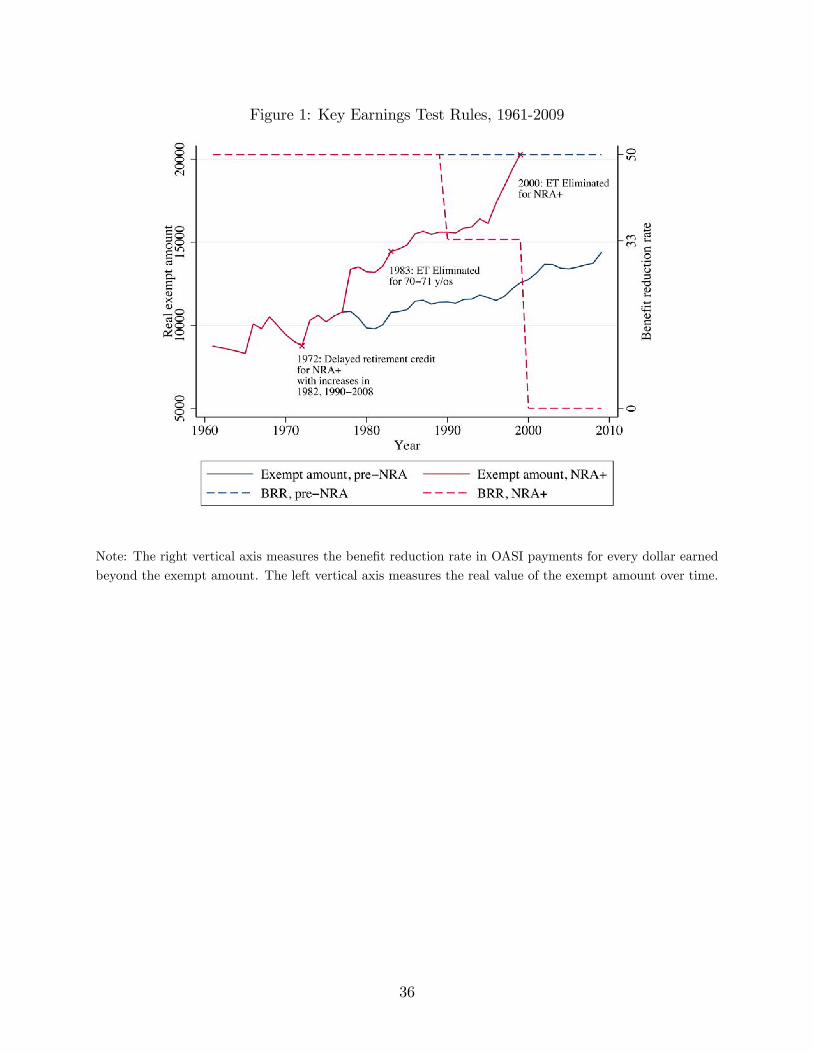
Figure 1: Key Earnings Test Rules, 1961-2009

Note: The right vertical axis measures the benefit reduction rate in OASI payments for every dollar earned

beyond the exempt amount. The left vertical axis measures the real value of the exempt amount over time.

36

Figure 2: Histograms of Earnings, 59-73-year-olds Claiming OASI by Age 65, 1990-1999

Notes: The bin width is $800. The earnings level zero, shown by the vertical lines, denotes the kink.

"Claimant" refers to an individual who has claimed by age 65.

37

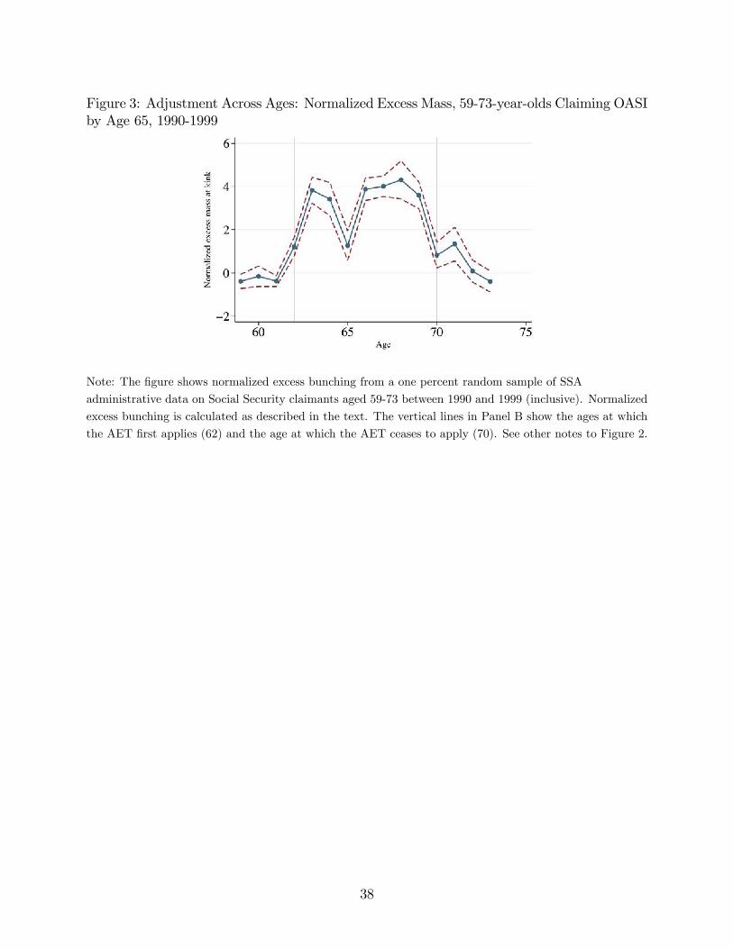
Figure 3: Adjustment Across Ages: Normalized Excess Mass, 59-73-year-olds Claiming OASIby Age 65, 1990-1999

Note: The figure shows normalized excess bunching from a one percent random sample of SSA

administrative data on Social Security claimants aged 59-73 between 1990 and 1999 (inclusive). Normalized

excess bunching is calculated as described in the text. The vertical lines in Panel B show the ages at which

the AET first applies (62) and the age at which the AET ceases to apply (70). See other notes to Figure 2.

38

Figure 4: Adjustment Across Years: Histograms of Earnings and Normalized Excess Mass,66-69 year olds Claiming OASI by Age 65, 1996-2004

Note: The figure shows histograms of earnings from a one percent random sample of SSA administrative

data on Social Security claimants aged 66-69 in each year from 1996 to 2004 (inclusive). In 2000 and after,

the (placebo) kink is defined as the kink applying to those in the year of attaining NRA; as we mention in

the text, the results are robust to two other ways of defining this placebo kink. See other notes to Figure 2.

39

Figure 5: Normalized Excess Bunching by Year, 1961-2005

Note: The figure shows normalized excess bunching from a one percent random sample of SSA

administrative data on Social Security claimants aged 66-69 in each year between 1961 and 2005. See other

notes to Figure 3.

40

Figure 6: Bunching Responses to a Convex Kink, with Fixed Adjustment Costs

Note: See Section 7 for an explanation of the figures.

41

Table 1: Summary Statistics, Social Security Administration Master Earnings File

(1) (2)

Ages 18-75 Ages 62-69

Mean Earnings 37,492.28 29,485.08(282,940.03) (783,897.87)

10th Percentile 5,234.74 1,957.7825th Percentile 15,291.11 7,291.2150th Percentile 32,982.17 17,739.6875th Percentile 46,949.86 38,149.9090th Percentile 66,370.18 58,417.99

Fraction with Positive Earnings 0.50 0.57

Fraction Male 0.56 0.57

Observations 13,612,313 1,595,139Individuals 619,580 545,615

Note: The data are taken from a one percent random sample of the SSA Master Earnings File and Master

Beneficiary Record. The data for ages 18-75 cover those in 1961-2005 who claim by age 65, who do not

report self-employment earnings, and who have positive earnings. (However, the fraction with positive

earnings is calculated by including those who have zero earnings.) Column 2 covers the same sample but

limits the ages to 62-69, the group we examine most often. Earnings are expressed in 2010 dollars.

Numbers in parentheses are standard deviations. The standard deviations are large because of very rare,

abberrant large values of earnings (as documented in Utendorf 2001/2); these do not affect our estimates in

the figures or tables because they are far above the AET exempt amount. These abberant values affect

mean earnings far less than they affect the standard deviation. The results are robust to winsorizing.

42

Table 2: Estimates of Elasticity and Adjustment Cost Using Sharp Change Method

(1) (2) (3) (4)

ε φ ε|φ = 0

1990 1989

Baseline 0.23 $152.08 0.39 0.22[0.20, 0.27]*** [49.54, 382.94]*** [0.33, 0.48]*** [0.18, 0.26]***

Lognormal density 0.26 $165.76 0.43 0.24[0.22, 0.30]*** [45.57, 473.52]*** [0.35, 0.54]*** [0.19, 0.29]***

Benefit Enhancement 0.39 81.52 0.59 0.37[0.33, 0.45]*** [18.11, 245.88]*** [0.49, 0.73]*** [0.30, 0.43]***

Excluding FICA 0.32 $129.14 0.50 0.30[0.27, 0.36]*** [34.18, 360.97]*** [0.42, 0.62]*** [0.25, 0.35]***

Bandwidth = $500 0.25 $90.65 0.38 0.24[0.21, 0.30]*** [6.04, 319.69]*** [0.30, 0.50]*** [0.19, 0.30]***

1988 to 1990 0.32 $114.33 0.50 0.31[0.29, 0.35]*** [26.49, 307.96]*** [0.42, 0.62]*** [0.27, 0.34]***

Note: The table shows estimates of the elasticity and adjustment cost using the Sharp Change method

described in the text. We report bootstraped confidence intervals shown in parentheses. We investigate the

1990 reduction in the AET BRR from 50 percent to 33.33 percent. The baseline specification assumes a

uniform density, calculates the effective MTR by including the effects of the AET BRR and federal and

state income and FICA taxes, and uses data from 1989 and 1990. Alternative specifications deviate fromthe baseline as noted. The estimates that include benefit enhancement use effective marginal tax rates due

to the AET based on the authors’calculations relying on Coile and Gruber (2001) (assuming that

individuals are considering earning just enough to trigger benefit enhancement). This translates the BRR

before and after the 1990 policy change to 36% and 24%, respectively. Columns (1) and (2) report joint

estimates with φ ≥ 0 imposed (consistent with theory, as described in the Appendix), while Columns (3)and (4) impose the restriction φ = 0. The constrained estimate in Column (3) only uses data from 1990,

whereas that in Column (4) uses only data from 1989 (except in the row where we investigate data from

1988 and 1990, in which case Column 4 uses data from 1988). *** indicates that the left endpoint of the 99

percent confidence interval is greater than zero; ** indicates that this is true for the 95 percent confidence

interval; and * for the 90 percent confidence interval.

43

A Appendix: Additional Features of Annual EarningsTest70

When current benefits are lost to the AET, future scheduled benefits are increased in somecircumstances. This is sometimes called "benefit enhancement." As we describe, for workersNRA or older in the pre-2000 period (when they faced the AET), benefit enhancementattenuates the effective AET BRR for individuals considering earning enough to trigger thebenefit enhancement, but it does not attenuate the effective AET BRR for those consideringearning less than this amount.The benefit enhancement rules have varied over time, and they depend on whether the

beneficiary is above or below NRA. Prior to 1972, there was no benefit enhancement forpeople aged NRA and older. In these years, the AET represented a pure loss in benefitsfor those NRA and above (equivalent to a pure tax). For beneficiaries NRA and older,a one percent Delayed Retirement Credit (DRC) was introduced in 1972. The DRC wasintended to compensate beneficiaries who delayed claiming beyond age 65, but they alsoapply to earnings lost to the AET. For individuals above NRA, benefits are increased 1/12of 1 percent for each month between ages 65 and 72 for which no benefits received after 1972(Social Security, 2012, Table 2.A.20).71

This language indicates that each month’s worth of foregone benefits– either because ofdelayed claiming or because of the AET– results in increased future benefits. A beneficiaryhas to forego an entire month of benefits in order to receive the DRC; if, for example, sheearns slightly over the exempt amount and loses only a small amount of benefits to theAET, then her future benefits are not adjusted. Thus, the DRC provides no marginal relieffrom the AET for a claimant who is considering earning near the exempt amount: no benefitenhancement occurs when she earns a marginal dollar at or near the AET earnings threshold.Meanwhile, if she earns enough to forego an entire month’s worth of benefits (but not whena smaller amount of benefits is lost due to the AET), future benefits are increased by 1/12of 1 percent.As a result of these rules, future benefits are enhanced when the individual’s yearly

earnings are over z∗ +(MB/τ), where z∗ is the exempt amount, MB is the monthly benefit,and τ is the AET benefit reduction rate.72 For example, with a typical monthly benefit of$1,000 and a benefit reduction rate of 33.33 percent, benefit enhancement occurs when theindividual’s yearly earnings are $3,000 (=$1000/0.3333) above the exempt amount. Benefitenhancement corresponding to one more month of reduced earnings occurs once annualearnings reaches $6,000 above the exempt amount, and so forth. Thus, benefit enhancementis only relevant to an individual considering earning substantially in excess of the exemptamount and is therefore not relevant to marginal earnings decisions at the exempt amount.

70This section is based on table 2.A.20 of the Annual Statistical Supplement of the Social Security bulletin,as well as extensive email correspondence with numerous offi cials at the Social Security Administration.71The size of the DRC was increased to three percent per year in 1982, and then increased steadily

throughout the 1990s, reaching eight percent for each year of foregone benefits in 2008. Starting in 1983,benefit enhancement only applied through age 69.72Another month’s benefit enhancement would occur if the individual earns more than z∗ +(2MB/τ); a

third month’s benefit enhancement would occur if she earns more than z∗ +(3MB/τ); and so on. Note thatthis creates 12 notches in the budget set, the final one at z∗ +(12MB/τ).

44

Indeed, this theoretical presumption is consistent with suggestive evidence we describe thatindicates little systematic bunching reaction to changes in the DRC and that mean age atdeath is smooth near the exempt amount.The AET is implemented in a number of stages. First, SSA must determine that

a claimant is expected to exceed the exempt amount, or that she has already done so.Claimaints can notify SSA in advance if they expect to exceed the exempt amount, or theycan report their earnings ex post facto at any point in the year. In addition, SSA usesW-2 records at the end of the year to determine if the AET threshold has been crossed(for those who have a W-2). Second, SSA withholds OASI benefits in monthly increments,until enough benefits have been withheld to cover the AET penalty amount. For example,assume an individual aged 66 with a monthly benefit of $1,200 earns $1,800 dollars beyondthe AET exempt amount in 1992, when the benefit reduction rate was 0.3333. This individ-ual should receive a yearly benefit reduction of $1,800 × 0.3333 = $600. SSA withholds anentire month’s check, $1,200, in order to collect the $600. Finally, at the end of the year,SSA refunds any overwithheld benefits. In the same example, at the end of the year SSAwould return $600 in overwithheld benefits. Importantly, the DRC is not applied to futurebenefits in this case– less than a month’s worth of benefits, $600, was ultimately collectedby SSA, after factoring overwithholding and refunds. After considering both withholdingand refunds, the AET is ultimately applied at a yearly level– much in the same way thatthe Earned Income Tax Credit (EITC) is applied at the annual level but the receipt of thecredit depends on one’s withholding patterns and when the income tax return is filed.In sum, for people NRA and older, the AET effectively acts as a kink for those earn-

ing close enough to the exempt amount, and benefit enhancement does not attenuate themarginal work disincentives associated with the AET in this range of earnings. However,the DRC is relevant to an individual considering earning enough to reduce her OASI benefitby at least a month’s worth (i.e. at least z∗ +(MB/τ)). Empirically, we find that limitingthe sample to those with substantial OASI benefits– for whom this earnings level is severalthousand dollars above the AET exempt amount, and for whom the notch created by theDRC is therefore less relevant– yields very similar results to those we have shown. Our em-pirical specification alternatively assumes that benefit enhancement does not affect the AETimplicit marginal tax rate (or does), and we find similar patterns in both specifications.Note that in our empirical estimation, the region we "dummy out" near the kink z∗

is [z∗ − 2800, z∗ + 2800]. Thus, if all of the "bunchers" arrived at the kink from initialearnings levels between z∗ and z∗ + 2800, we could find zero bunching despite substantialactual bunching. However, the earnings densities clearly show that the polynomial does notsubstantially overpredict bunching in the region above the exempt amount. Moreover, thedensities also show no evidence of bunching near notches in the budget set created by theDRC. We alternatively use a bandwidth of $500 and find similar results.Individuals younger than NRA are subject to different rules for benefit adjustment, called

"actuarial adjustment." The rule for this younger group was introduced in the legislationallowing people younger than 65 to claim early benefits (in 1956 for women and in 1961for men). For those younger than NRA, future benefits are reduced 5/9 of 1 percent foreach month under age 65 in which an individual claims benefits (Social Security, 2012, Table2.A.20). This implies that if a beneficiary has any income withheld under the AET in a givenmonth, then she receives a full benefit enhancement for that month. On the other hand,

45

if a beneficiary does not have any income withheld under the AET in a given month, thenshe receives no benefit enhancement for that month. This creates a notch at the exemptamount– a discontinuous increase in future benefits when moving from just under the exemptamount to just over it– creating incentives to bunch just above the exempt amount in orderto receive the monthly (or yearly) benefit adjustment. We find no evidence for this kind ofbehavior; in fact, as we document in Gelber, Jones, and Sacks (2013), people tend to haveearnings just below the exempt amount, exactly opposite the behavior we would expect ifpeople were responding to the notch just described. Because benefit enhancement occurs atexactly the same earnings level that the AET begins to apply for those under NRA, we focuson the group NRA and above.Formally, the number of months’worth of benefit enhancement enjoyed by OASI recip-

ients is therefore floor(τ · (z − z∗)/MB) for those NRA and above, and ceiling(τ · (z −z∗)/MB) for those below NRA.Benefit enhancement is actuarially fair if the net present value of the benefit enhancement

equals the benefits lost due to the AET. The actuarial adjustment is approximately actuari-ally fair in the sense that delaying OASI claiming an extra year is approximately actuariallyfair ; however, this does not imply that benefit enhancement is actuarially fair when an ad-ditional dollar of benefits is withheld due to the AET. For example, actuarial adjustment isnot actuarially fair for (among others) those with positive OASI benefits considering earningan additional amount above the AET exempt amount, because this does not result in addi-tional benefit enhancement. Similar considerations apply to the DRC: additional marginalincrements of earnings are not compensated through benefit enhancement (except in thecase when an individual goes from earning just under to just over z∗ +(MB/τ) (or one ofthe other 12 thresholds)).The AET applies to an individual’s earnings; spouses’earnings do not count in the earn-

ings total to which the AET is applied. For a retired worker (i.e. primary) beneficiary whosespouse collects spousal benefits, the AET reduces the family’s OASI benefit by the amountswe have described. The family benefit is also reduced when the spouse (separately) earnsmore than the AET threshold. For a retired worker beneficiary whose spouse is collectingbenefits on his or her own earnings record, the AET reduces the retired worker beneficiary’sbenefits by the amounts described while not affecting the spouse’s benefits. Thus, followingprevious literature (e.g. Friedberg 1998, 2000), we model the AET as creating the MTRsassociated with the BRRs described, because the AET reduces family benefits by theseamounts (all else equal). Our data do not contain the information necessary to link spouses(except when one spouse is claiming OASI benefits on the other spouse’s record).It is also worth noting how the actuarial adjustment and DRC interact with incentives for

claiming OASI. Under the actuarial adjustment, the full benefit enhancement occurs whenthe individual earnings over the threshold level. Thus, the individual could in principleclaim OASI; earn just over this threshold level; collect nearly her entire OASI benefit in thisyear (since the AET only reduces current OASI benefits at the margin); and later enjoy fullbenefit enhancement. This illustrates the more general point that it can be in an individual’sinterest to claim OASI even if the individual faces the AET. More generally, for individualsfor whom the AET reduces OASI benefits suffi ciently little, and for whom current OASIbenefits are suffi ciently important, it can be in their interest to claim OASI even if they facethe AET. Appendix Figure F.22 shows that among the sample of individuals who have not

46

claimed by year t, the hazard of claiming at year t + 1 is smooth near the kink, indicatingno evidence that claimants come disproportionately from close to or far from the kink.

B Appendix: Procedure for Estimating Normalized Ex-cess Bunching

In order to estimate excess normalized bunching, we use the following procedure. For eachcentered-earnings bin zi, we calculate pi, the proportion of all people with earnings in therange [zi − k/2, zi + k/2) (in a given time period and for a given age group). For example,underlying the first panel in Figure 2 is the probability pi of earning in various bins zi for62 year-olds in the 1990-1999 period. The earnings bins are normalized by distance-to-kink,so that for zi = 0, pi is the fraction of people with earnings in the range [−k/2, k/2). Toestimate bunching, we assume that pi can be written as

pi =

D∑d=0

βd(zi)d +

k∑n=−k

γk1{zi = kδ}+ εi (B.1)

and run this regression. This equation expresses the earnings distribution as a degree Dpolynomial, plus a set of indicators for each bin within kδ of the kink, where δ is thebinwidth. In our empirical application, we choose D = 7, δ = 800 and k = 3 (so that sevenbins are excluded from the polynomial estimation, including the bin centered at the kink).We show that our results to alternative choices of D, δ, and k.Our measure of excess mass is ˆEM =

∑kn=−k γk, the estimated excess probability of

locating at the kink (relative to the polynomial term). This measure depends on the coun-terfactual density near the kink, so to obtain a measure of excess mass that is comparableat the kink, we scale by the predicted density that would obtain if there were no bunching.This is just the constant term in the polynomial, since the zi is distance to zero. So ourestimate of normalized excess mass is

B =ˆEM

β0

. (B.2)

We consider two approaches for constructing standard errors. First, from Equation (B.2), itis straightforward to apply the Delta method. Second, we employ the parametric bootstrapprocedure of Chetty, Friedman, Olsen and Pistaferri (2011). This bootstrap draws withreplacement from the estimated distribution of errors εi from Equation (B.1). For each setof draws, we get a new value of pi and use these new values to re-estimate B. The standarddeviation across draws of B is our measure of the standard error B. In practice these twoprocedures produced extremely similar results, so we only report standard errors from thebootstrap.

C Appendix: Social Security DataOur data come from the Social Security Master Earnings File (MEF), which is describedmore extensively in Song and Manchester (2007). The MEF is a longitudinal history ofSocial Security taxable earnings for all Social Security Numbers (SSNs) in the U.S. Our data

47

are a one percent random sample of SSNs; we randomly extract SSNs from the databaseand follow each of these individuals over the full time period. The AET is based on earningsas measured in this dataset. Prior to 1978, the data have information on annual FICAearnings; since 1978, the data have information on uncapped wage compensation. Before1978, the data do not clearly distinguish between earnings from self-employment and non-self-employment earnings, but we are able to distinguish them in the data starting in 1978.The data also contain information on date of birth, date of death, and sex.We supplement the MEF with information from the Master Beneficiary Record (MBR)

file, which contains data on the day, month, and year that people began to claim SocialSecurity (and other variables). The majority of workers excluded from OASDI coverage arein four main categories: (1) federal civilian employees hired before January 1, 1984; (2)agricultural workers and domestic workers whose earnings do not meet certain minimumrequirements; (3) individuals with very low net earnings from self-employment (generallyless than $400 per year); and (4) employees of several state and local governments. However,civil service and other government workers are covered by Medicare and are therefore presentin the MBR.In choosing our main sample, we take into account a number of considerations. It is

desirable to show a constant sample in making comparisons of earnings densities. Meanwhile,the AET only affects people who claim OASI, and thus we wish to focus on claimants.However, many individuals claim OASI at ages over the Early Entitlement Age (62), implyingthat they have not claimed at younger ages but have claimed by older ages. This impliesthat to investigate a constant sample, we cannot simply limit the sample to claimants ateach age (because many people move from not claiming to claiming). To balance theseconsiderations, our main sample at each age and year consists of individuals who ultimatelyclaim in the year they turn 65 or earlier. We show that the results are robust to othersample definitions. Because we focus on the intensive margin response (consistent with Saez(2010) and subsequent papers on bunching), we further limit the sample to observations withpositive earnings in our main analysis.Information on AET parameters is from table 2.A.20 and 2.A.29 of the Annual Statistical

Supplement to the Social Security Bulletin. Friedberg (1998, 2000) provides a thoroughdescription of these rules. All dollar amounts are deflated to 2010 dollars using the CPI-U.The standard deviation is large because of very rare abberrant large values of earnings

(as documented in Utendorf 2001/2); these do not affect our estimates in the figures or tablesbecause they are far above the AET exempt amount, and they affect mean earnings far lessthan they affect the standard deviation. The results are robust to winsorizing.In 1983-1999, the AET is assessed on earnings until the month in which the individual

turns age 70. For simplicity, in our baseline sample we measure age as calendar year minusyear of birth. Thus, if an individual turns age 70 later in the year– in the extreme case, onDecember 31– she will have had an incentive to bunch at the kink during nearly the entireyear when she is classified as age 70 in our data. As a result, her yearly earnings may appearto be located at or near the kink even though she is bunching at the kink applicable to69-year-olds through almost all of the calendar year over which her earnings are observed.However, the figure shows that significant bunching occurs at age 71, which cannot be due tothis coarse measure of birth dates. Thus, the results do show a delay in complete adjustment.We have also found substantial and significant (p < 0.01) bunching at age 70 among those

48

born in January, who no longer face the AET immediately in January of the year they turn70 and therefore should not show excess bunching at this age in the absence of adjustmentfrictions. Likewise, we find a spike in mean earnings growth from age 70 to age 71 amongthose born in January. In our sample period, the AET applied to ages 62-71 before 1983,and it applied to ages under NRA in 2000 and after. In these time periods, examining onlythose born in January also shows a delay in responding to the removal of the AET.Since 1978, the earnings test has been assessed on yearly earnings, implying that we

analyze the appropriate time period, i.e. earnings in a calendar year. Prior to 1978, theearnings test was assessed on quarterly earnings. While there is likely some error in measuringthe amount of bunching pre-1978, we believe that this is not a major issue: the patterns ofbunching in the pre-1978 period are visually clear and appear unlikely to be changed in aqualitative sense by an examination of quarterly data. Moreover, Figure 5 shows that theamount of excess bunching falls from 1977 to 1978 and subsequent years, rather than risingas we might expect if we hypothetically measured bunching more accurately starting in 1978.

D Appendix: Longitudinal Employer Household Dy-namics

We use the Longitudinal Employer Household Dyanmics (LEHD) dataset, which containswage data available from state-level unemployment insurance (UI) programs. These datameasure uncapped quarterly earnings for employees covered by state unemployment insur-ance systems, estimated to cover over 95 percent of private sector employment. Althoughcoverage laws vary slightly from state to state, UI programs do not cover federal employees,the self-employed, and many agricultural workers, domestic workers, churches, nonprofits,and state and local government employees. We examine a 20 percent random sample of theoriginal LEHD file, as this was the largest amount of data that our available server spacecould handle.These administrative earnings records are linked across quarters to create individual work

histories. In addition to earnings, information on gender and date of birth are available. Thedata on employees are linked to data on firms. Each firm at which an individual works ina given quarter is identified through a firm identifier. We consider an employee to havechanged employers from year t to year t + 1 if at least one of the federal employer IDs atwhich the employee works in year t is different in year t + 1. However, when the individualworks at one or more employer in year t and does not work at any employer in year t+ 1, wedrop this individual from the sample. The results are similar when we treat these individualsas if they changed employers.We select data from 1990-1999. During this period, the AET explicit benefit reduction

rate was constant. 1990-1999 also represent natural years to investigate because large samplesizes are not available in the LEHD prior to 1990. When we include other years and agegroups in the LEHD sample, we find similar results to those reported here. Note that thepopulation we investigate is not constant over this period, because (among other reasons) anincreasingly broad set of states is included in the LEHD over time. Data are available on 13states in 1990, climbing to 28 states by 1999. In a given quarter, we include in our sampleall states whose data are available. Holding the sample constant yields very similar results.

49

E Appendix: Model of Earnings ResponseE.1 Baseline ModelWe start with a baseline, frictionless model of earnings, following Saez (2010). We brieflysketch the key features of this model for comparison to our model with a fixed cost ofadjustment. In Saez (2010), individuals maximize utility over consumption, c, and costlyearnings, z:

u (c, z;n)

Heterogeneity is parameterized by an "ability" parameter n, which is distributed according tothe smooth cdf F (·). Individuals maximize utility subject to the following budget constraint:

c = (1− τ) z +R

where R is virtual income. This leads to the first order condition:

−uz (c, z;n)

uc (c, z;n)= (1− τ) ,

which implicitly defines an earnings supply function: z (1− τ , R, n).When necessary, we will use a quasi-linear and iso-elastic utility function:

u (c, z;n) = c− n

1 + 1/ε

( zn

)1+1/ε

Under this assumption, the first order condition simplifies to:

(1− τ)−( zn

) 1ε

= 0,

which implies this earnings supply function:

z = n (1− τ)ε .

E.2 Linear Tax ScheduleConsider first a linear tax schedule with a constant marginal tax rate τ 0. Observe that with asmooth distribution of skills n, we have a smooth distribution of earnings that is monotonicin skill, provided we make the typical Spence-Mirlees assumption. Let H0 (·) denote thecumulative distribution function (CDF) of earnings under the constant marginal tax rate,and let h0 (·) = H ′0 (·) denote the density of this distribution. Under quasilinear utility, wehave:

H0 (z) = F

(z

(1− τ 0)ε

).

Define H1 (·) and h1 (·) as the smooth CDF and density of earnings under a higher, constantmarginal tax rate τ 1; H1 is defined similarly as a function of τ 1.

50

E.3 Kinked Tax ScheduleNow consider a piecewise linear tax schedule with a convex kink: the marginal tax rate belowearnings level z∗ is τ 0, and the marginal tax rate above z∗ is τ 1 > τ 0. Given the tax schedule,individuals bunch at the kink point z∗; as explained in Saez (2010), the realized density inearnings has an excess mass at z∗. Denote the realized distribution of earnings once the kinkhas been introduced at z∗ as H (·):

H (z) =

{H0 (z) if z < z∗

H1 (z) if z ≥ z∗

Denote the density of this realized distribution as h (·) = H ′ (·). In general there is now adiscrete jump in the earnings density at z∗:

h (z) =

{h0 (z) if z < z∗

h1 (z) if z > z∗

The share of people who relocate to the kink is:

B =

∫ z∗+4z∗

z∗h0 (ζ) dζ

These "bunchers" are those whose ex ante earnings lie in the range [z∗, z∗ +4z∗], who areinduced to locate at the kink by the rise in the MTR above the kink point. For relativelysmall changes in the tax rate, we can relate the elasticity of earnings with respect to the net-of-tax rate to the earnings change 4z∗ for the individual with the highest ex ante earningswho bunches ex post :

ε =4z∗/z∗

dτ 1/ (1− τ 0)

where dτ 1 = τ 1 − τ 0.73

E.4 Graphical ExpositionAppendix Figure F.1 depicts a setting in which a kinked budget set is introduced. In PanelsA and B, the x-axis shows before-tax-and-transfer income, z, and the y-axis shows after-tax-and-transfer consumption, z−T (z). Consider first a linear tax (Panel A) at a rate of τ . Anindividual optimally locates at a point of tangency, where the marginal rate of substitution(MRS) between earnings and consumption equals the net-of-tax rate, 1−τ . The figure showsindifference curves and earnings levels for low- and high-earning agents (labeled L and H,respectively). The low earner has an earnings level of z∗, while the high earner receivesz∗ +4z.Suppose the AET is introduced (on top of pre-existing taxes), so that the marginal net-of-

tax rate decreases to 1− τ − dτ for earnings above a threshold z∗. For small dτ , individualsearning in the neighborhood above z∗ will reduce their earnings. If ability is smoothlydistributed, a range of individuals will locate exactly at z∗, due to the discontinuous jump

73This formula holds if there is a single elasticity ε in the population. Under heterogeneity, the methodreturns ε, the average elasticity among bunchers. We investigate cases with heterogeneity below.

51

in the marginal net-of-tax rate at z∗. In Panels A and B, individual L has the lowest ex anteearnings among those who bunch at z∗, individual H has the highest ex ante earnings in thisgroup, and all others previously earning between z∗ and z∗ +4z also bunch at z∗. Thosewith ex ante earnings higher than z∗ +4z reduce their earnings to a level greater than z∗.Panels C and D of Figure F.1 depict densities of earnings we would expect to observe in

the absence and presence of the AET, respectively. The x-axis shows before-tax earnings, z,and the y-axis measures the density of earnings. In Panel C, the density is continuous at z∗,reflecting a smooth distribution of ability. The blue region represents the set of individualswho bunch at z∗ in the presence of the AET, i.e. those earning in [z∗, z∗ +4z] in the absenceof the AET. Panel D shows that once the AET is introduced, these individuals locate in theneighborhood of z∗. However, rather than depicting a mass point exactly at z∗, we haveshown bunching in the region at and surrounding z∗, reflecting the fact that individualsoften cannot bunch exactly at the kink point (as discussed, for example, in Saez, 2010).

E.5 Fixed Adjustment CostsWe now extend the model to include a fixed cost of adjusting earnings. We assume thatthe adjustment cost reflects a disutility of φ∗ of increasing or decreasing earnings from someinitial earnings level. We begin by analyzing the response to a change in the marginal taxrate from τ 0 to τ 1, where the tax schedule is linear in both cases, in order to build intuitionfor the case with a kinked budget set. We assume that following a change in tax rates fromτ 0 to τ 1, the gain (absent adjustment costs) to reoptimizing is increasing in n. In general,this requires that the size of the optimal earnings adjustment increases in n at a rate fasterthan the decrease in the marginal utility of consumption.74 This is true, for example, ifutility is quasilinear.If the gain in utility is monotonically increasing in initial earnings, and the cost of adjust-

ment is fixed, there exists a unique level of initial earnings at which the agent is indifferentbetween adjusting and staying at the initial earnings level. We formally state the implicationsin the following result:

Remark 1 (Linear Tax Change and Adjustment Costs)

After a change in linear tax rates from τ 0 to τ 1, if there is a constant adjustment cost ofφ∗ and the size of the optimal earnings adjustment increases in n at a rate faster than thedecrease in the marginal utility of consumption, then:

1. There is a unique threshold of initial earnings, z0,φ, above which all individuals willadjust their earnings in response to the tax change. Those initially locating below thethreshold will not adjust.

74To see this, note that the utility gain from reoptimizing is u ((1− τ1) z1 +R1, z1;n) −u ((1− τ1) z0 +R1, z0;n) ≈ uc · (1− τ1) [z1 − z0] + uz · [z1 − z0] = uc · (τ1 − τ0) [z0 − z1], where in thefirst expression, we have used a first-order approximation for utility at ((1− τ0) z0 +R0, z0) and in the sec-ond expression we have used the first order condtion uz = −uc (1− τ0). The gain in utility is approximatelyequal to an expression that depends on the marginal utility of consumption, the change in tax rates, andthe size of the earnings adjustment. The first term, uc, is decreasing as n (and therefore initial earnings z0)increases. Thus, in order for the gain in utility to be increasing in n, we need the size of earnings adjustment[z0 − z1] to increase at a rate that dominates.

52

2. The threshold level of earnings satisfies the following identity:

u ((1− τ 1) z1,φ +R1, z1,φ)− u ((1− τ 1) z0,φ +R1, z0,φ) ≡ φ∗

where z1,φ is the ex post earnings level of the individual who initially locates at z0,φ.In other words, at the threshold level, the gain in u from adjusting earnings is exactlyequal to the adjustment cost φ∗.

3. In the case of quasilinear utility, the threshold level of earnings is:

z0,φ =φ∗

α (ε, τ 0, τ 1)

where

α (ε, τ 0, τ 1) ≡ 1− τ 1

1 + ε

[(1− τ 1

1− τ 0

)ε− 1 + ε

(τ 1 − τ 0

1− τ 1

)].

4. The ex post distribution of earnings is:

H (z) =

H0 (z) if z < z1,φ

H0 (z) +H1 (z)−H0 (z0,φ) if z ∈ [z1,φ, z0,φ]H1 (z) if z > z0,φ

h (z) =

h0 (z) if z < z1,φ

h0 (z) + h1 (z) if z ∈ [z1,φ, z0,φ]h1 (z) if z > z0,φ

where H0 (·) and H1 (·) are the CDFs of earnings in the presence of linear tax rates τ 0

and τ 1, respectively.

Next, consider choices in the presence of adjustment costs on a budget set with a convexkink. Consider again an initial linear tax schedule with marginal tax rate τ 0. Now, introducea higher MTR τ 1 > τ 0 for earnings above z∗. We again assume that the gain to reoptimizingis increasing in initial earnings over the range [z∗, z∗ +4z∗]. Using the same logic as above–the gain in utility is monotonically increasing in initial earnings, and the cost of adjustment isfixed– there exists a unique level of initial earnings at which the agent is indifferent betweenadjusting and staying at the initial earnings level. Thus, we have the following result:

Remark 2 (Non-Linear Tax and Adjustment Costs)

When a kink is introduced in the budget set (i.e. a jump in marginal tax rates from τ 0

below z∗ to τ 1 above z∗), there is a fixed adjustment cost of φ∗, and z∗ ≥ z1,φ,75 then:

1. Individuals with initial earnings below a unique threshold z do not adjust their earnings.

75z1,φ is again the ex post level of earnings for the individual who initially locates at z0,φ —where z0,φ isthe initial earnings level over which individuals adjust their earnings defined above in Remark (1). Note thatz denotes this threshold in the non-linear budget set case, whereas z0,φ denotes this threshold in the linearbudget set case.

53

2. The threshold level of earnings is implicitly defined by the following:

u ((1− τ 1) z∗ +R1, z∗)− u ((1− τ 1) z +R1, z) ≡ φ∗ (E.3)

z∗ ≤ z ≤ z∗ +4z∗.

3. Individuals with intial earnings in [z, z∗ +4z∗] bunch at the kink point z∗.

4. Individuals with initial earnings above z∗+4z∗ reduce their earnings to a new level ofearnings higher than z∗.

5. The ex post distribution of earnings is:

H (z) =

H0 (z) if z < z∗

H0 (z) +H1 (z)−H0 (z) if z ∈ [z∗, z]H1 (z) if z > z

h (z) =

h0 (z) if z < z∗

h0 (z) + h1 (z) if z ∈ [z∗, z]h1 (z) if z > z

6. Excess bunching at z∗ is given by:

B =

∫ z∗+4z∗

z

h0 (ζ) dζ

If the kink point z∗ is lower than z1,φ, then:

1. Individuals only adjust their earnings if their initial earnings level is above the thresholdz0,φ.

2. There is no bunching at z∗.

3. The ex post distribution of earnings is the same as in the case of a change in a lineartax rate from τ 0 to τ 1 described in Remark (1).

E.6 Derivation of Closed-Form Solution for Elasticity and Adjust-ment Cost (Comparative Static Approach)

As we discuss in Remark (2) above and in Section 7 in the text, the amount of bunching inthe presence of a fixed adjustment cost is equal to the integral of the initial earnings densityover the range [z, z∗ + ∆z∗]:

B(τ , z∗; ε, φ∗) =

∫ z∗+∆z∗

z

h (ζ) dζ, (E.4)

where τ ≡ (τ 0, τ 1). If the density is locally uniform, the integral in (E.4) is:

B(τ , z∗; ε, φ∗) ≈ h(z)(z∗ + ∆z∗ − z) (E.5)

54

Taking a first-order Taylor approximation of u ((1− τ 1)z +R1, z, n) and u ((1− τ 1)z∗ +R1, z∗, n)

at ((1− τ 0)z +R0, z, n), and using the first order condition for initial earnings, (1− τ 0)uc =−uz, we have from (E.3):

φ∗ ≈ uc · (1− τ 1) [z∗ − z] + uz · (z∗ − z)

⇒ z ≈ z∗ +φ∗/uc

(τ 1 − τ 0)

= z∗ +φ

dτ 1

,

where dτ 1 = τ 1 − τ 0 and φ = φ∗/uc is the dollar equivalent of the disutility associated withadjusting earnings. Substituting this expression for z into (E.5), we have

B(τ , z∗; ε, φ) = h(z)(∆z − φ/dτ 1),

where bunching now depends on the dollar-denominated cost of adjusting, rather than theutility cost. Finally, for small dτ , ∆z is small and h(z) ≈ h(z∗ + ∆z) ≈ h(z∗). Let b ≡B/h(z∗), and note that ∆z∗ = z∗ (dτ 1/ (1− τ 0)) ε. The excess mass at the kink can now beexpressed as a linear function of the parameters:

b(τ , z∗; ε, φ) = ε

(z∗

dτ 1

1− τ 0

)− φ

(1

dτ 1

). (E.6)

E.6.1 Derivation of Formula for Bunching with Heterogeneity

We derive the formula for bunchingB in the presence of heterogeneity under the ComparativeStatic approach as follows:

B =

∫∫∫ z∗+∆z∗

z

h (ζ, ε, ϕ) dζdεdϕ

≈∫∫

[z∗ + ∆z∗ − z] h (z∗, ε, ϕ) dεdϕ

≈∫∫ [

ε

(z∗

dτ 1

1− τ 0

)− ϕ

(1

dτ 1

)]h (z∗, ε, ϕ) dεdϕ

= h (z∗) ·[(∫∫

εh (z∗, ε, ϕ)

h (z∗)dεdϕ

)(z∗

dτ 1

1− τ 0

)−(∫∫

ϕh (z∗, ε, ϕ)

h (z∗)dεdϕ

)(1

dτ 1

)]

= h (z∗) ·[ε

(z∗

dτ 1

1− τ 0

)− φ

(1

dτ 1

)],

where we have used the assumption of constant h (·) and the approximations for ∆z∗ and zin Section 7. Here h (z∗) =

∫∫h (z∗, ε, ϕ) dεdϕ, and ε and φ are the average elasticity and

adjustment cost, respectively.

55

E.6.2 Linear Adjustment Costs

We now introduce an adjustment cost that increases linearly in the size of the adjustment.Assume that given an initial level of earnings z0, agents must pay a cost of φ

∗ · |z − z0|when they change their earnings to a new level z. Utility u at the new earnings level can berepresented as:

u (c, z;n, z0) = u (c, z;n)− φ∗ · |z − z0| .The first order condition for earnings can be characterized as:

−uz (c, z;n)

uc (c, z;n)= (1− τ − φ∗/λ∗ · sgn (z − z0))

=

{(1− τ − φ) if z > z0

(1− τ + φ) if z < z0,

where λ∗ = uc (c∗, z∗;n) is the Lagrange multiplier and φ = φ∗/λ∗ is the dollar equivalent ofthe linear adjustment cost φ∗.The individual chooses earnings as if he faces an effective marginal tax rate of τ =

τ + φ·sgn(z − z0). It follows that our predictions about earnings adjustment are similar toour previous predictions, except that the effective marginal tax rate τ appears, rather thanτ . Thus, we can solve for the elasticity of earnings as a function of the change in earnings4z∗ due to introduction of a kink in the tax schedule and the jump in marginal tax ratedτ 1:

ε =4z∗/z∗

dτ 1/ (1− τ 0)

=4z∗/z∗

(dτ 1 − 2φ) / (1− τ 0 − φ).

Since the right-hand side is increasing in φ, the estimate of the elasticity increases as thelinear adjustment cost increases. This makes intuitive sense: the adjustment cost attenuatesbunching, so holding constant the level of bunching, the elasticity must be higher as theadjustment cost increases.Now assume that when an individual adjusts his earnings, he incurs a linear adjustment

cost φ∗L for every unit of change in earnings, as well as a fixed cost φ∗F associated with anychange in earnings. Consider again bunching at z∗, with a tax rate jump of dτ 1 = τ 1 − τ 0

at earnings level z∗. We have the following set of expressions for excess mass:

B =

∫ z∗+4z∗

z

h (ζ) dζ

ε =4z∗/z∗(

dτ 1 − 2φL)/(1− τ 0 − φL

)φ∗F + φ∗L · (z − z∗) = u

((1− τ 1) z∗ +R

′, z∗;n

)− u

((1− τ 1) z +R

′, z;n

).

56

Using a left rectangle approximation for the integral, we have:

b ≡ B/h (z∗)

= z∗ +4z∗ − z

= z∗(dτ 1 − 2φL

1− τ 0 − φLε+ 1

)− z.

We can further apply an approximation for z similar to the approximation we used in Section7, i.e. z = z∗ + φF/

(dτ 1 − 2φL

). Thus, the expression for bunching can be simplified to:

b = ε

(z∗

dτ 1 − 2φL

1− τ 0 − φL)− φF(

dτ 1 − φL) ,

where(φF , φL

)=(φ∗F/λ∗, φ∗L/λ∗

). In this case, we need at least three kinks to separately

identify(ε, φF , φL

). Because we do not examine a setting in which one can compare bunching

under three different positive tax rates, we are not able to estimate these parameters usingdata (or to fruitfully estimate the parameters in the non-linear case since we do not have acredible source of variation to identify them).

E.7 Derivation of Formula for Bunching with a Pre-Existing Kink(Sharp Change Approach)

The Comparative Static approach abstracts from a key feature of our empirical setting. Inparticular, the Comparative Static approach models the transition from a budget set withno kink to one with a kink. This approach facilitates our basic intution and provides atransparent bridge between our approach and existing bunching methods in the presenceof a kink. However, in our context, we conduct analysis using data just before and justafter the benefit reduction rate was decreased (in 1990 from 50 percent to 33.33 percent for66-69 year olds; or from 33.33 percent to zero for this group in 2000; or from 33.33 percentfor 69-year-olds to zero for 70-year-olds in 1990-1999). These changes involve moving froman initial state with a kink to a new state with a smaller kink. In a frictionless model,the distinction is immaterial. However, as we show, this matters in the presence of a fixedadjustment cost. In particular, when the kink becomes more muted, the change in bunchingwill be attenuated due to the fixed adjustment cost.We will assume that in the initial state, bunching is characterized as in Remark (2). Let

the initial kink, K1, be characterized by a lower marginal tax rate, τ 0, to the left of z∗, anda higher marginal tax rate, τ 1, to the right of z∗. The initial level of bunching is:

B1 =

∫ z∗+∆z∗1

z1

h (ζ) dζ

Now, consider a change in the kink to K2, which retains the lower marginal tax rate τ 0 tothe left of z∗ but reduces the marginal tax rate to the right of z∗ to τ 2 < τ 1. Had we begun

57

with no kink and introduced K2, bunching would have been:

B2 =

∫ z∗+∆z∗2

z2

h (ζ) dζ

Note that relative to K1, K2 provides a weaker incentive to bunch, when starting from abaseline tax schedule with no kink. Formally, we have z2 ≥ z1, ∆z∗2 < ∆z∗1 and B2 ≤ B1.

E.7.1 Characterizing Bunching

In characterizing bunching when moving from K1 to K2, individuals may be separated intoseveral groups based on their optimal level of earnings z0 in the absence of a kink. First,there are individuals with z0 < z∗. They will locate to the left of the kink under both K1

and K2.Second, we have individuals with z∗ < z0 ≤ z1 (area i in Figure 6). These individuals

would optimize in the presence of K1 by moving to z∗, were it not for the adjustment cost.Now, with a smaller kink K2, these individuals continue to remain at the initial earningslevel z0 > z∗, as the utility gain to reoptimizing to z∗ is even smaller than it was under K1.Third, we have those with z1 < z0 ≤ z2 (area ii in Figure 6). When moving from no

kink to K1, these individuals locate at the kink, z∗. If the budget set had hypotheticallytransitioned from no kink to K2, these individuals would have chosen to remain at z0, dueto the fixed adjustment cost. However, when moving from K1 to K2, these agents remain atthe kink z∗. The reason is that the frictionless optimum under K2 is z∗ for everyone initiallyearning in the range [z∗, z∗ + ∆z2].Fourth, we have agents with z2 < z0 ≤ z∗+ ∆z2 (area iii in Figure 6). These individuals

bunch at z∗ when moving from no kink to either K1 or K2. Thus, they remain bunching atz∗ when moving from K1 to K2.Fifth, we have agents with z∗+ ∆z2 < z0 ≤ z∗+ ∆z1 (areas iv and v in Figure 6). When

starting from a budget set with no kink, these agents bunch under K1, but not under K2.Starting instead from K1, they must choose between remaining at the kink z∗ or moving tothe frictionless optimum under K2, z2 > z∗. We know that at least some of these individualswill remain bunching. To see this, consider an individual with earnings under no kink z0 =z∗ + ∆z2 + δ0. For small enough δ0 optimal earnings under K1 is z∗, and optimal earningsunder K2 tends to z∗ as δ0 tends to zero. Likewise, the net utility gain from relocatingfrom z∗ to z2 under K2 tends to zero as δ0 tends to zero. However, the fixed adjustmentcost remains strictly positive. Therefore, this individual will remain at z∗ when movingfrom K1 to K2 for small enough δ0. In Figure 6, area iv shows those with initial earningsz∗ + ∆z2 < z0 < z0 who remain bunching at the kink when transitioning from K1 to K2.Area v shows those with initial earnings z0 < z0 < z∗ + ∆z1, who "debunch" from the kinkwhen moving from K1 to K2.When reoptimizing is beneficial for at least some agents in this final group, we will have

a reduction in bunching when transitioning from K1 to K2.76 Empirically, we observe sucha reduction over time, so this is the case relevant to our setting. In this case, the marginal

76In certain cases, it is possible that reoptimizing away from the kink is not optimal for anyone in theinitial earnings range [z∗ + ∆z2, z

∗ + ∆z1]. In that case, there is no change in bunching when moving fromK1 to K2.

58

"de-buncher" will be defined by the following conditions:

−uz (c2, z2; n2)

uc (c2, z2; n2)= (1− τ 2)

u ((1− τ 2) z2 +R2, z2; n2)− u ((1− τ 2) z∗ +R2, z∗; n2) ≡ φ∗

−uz (c0, z0; n2)

uc (c0, z0; n2)= (1− τ 0)

z0 ≤ z∗ + ∆z∗1

In words, the first line indicates that z2 > z∗ is the optimal, frictionless level of earningschosen by the top buncher in the presence of K2. The second line requires that when facingK2, this agent is indifferent between remaining at z∗ and moving to z2 through paying theadjustment cost. The third line defines z0 as the initial level of earnings that this individualchooses when facing a constant marginal tax rate of τ 0 and no kink. The fourth line requiresthat this individual is initially bunching at z∗ in response to K1. If this last inequality isbinding, then when moving from K1 to K2, none of the bunchers "debunch" and the fractionbunching is unchanged. In that case, we have no variation available to identify both ε andφ. As noted above, empirically we do observe that excess bunching falls around 1990 whenthe BRR falls from 50 percent to 33.33 percent (as well as in the other cases we examineempirically, in which the BRR falls from a positive level to zero). Thus, we restrict attentionto the case in which z0 < z∗ + ∆z1.Bunching at K2 following K1, when z0 < z∗ + ∆z1, can therefore be expressed as:

B2 =

∫ z0

z1

h (ζ) dζ

We can again solve this system of equations for φ∗ and ε. Note that ε is still identified bythe potential adjustment of the top-most buncher:

ε =z0 − z2

z2

(1− τ 0)

dτ 2

Note that when moving from K1 to K2, the change in bunching is smaller than it wouldbe if we had started with steady state bunching atK1 following no kink (B1) and then movedto steady state bunching K2 following no kink (B2). That is:

B1 − B2 =

∫ z∗+∆z∗1

z1

h (ζ) dζ −∫ z0

z1

h (ζ) dζ

≤∫ z∗+∆z∗1

z1

h (ζ) dζ −∫ z∗+∆z∗2

z2

h (ζ) dζ

= B1 −B2,

where the second line follows from the fact that z0 ≥ z∗ + ∆z∗2 and z1 ≤ z2.

59

E.7.2 Simplified Approximation

We can again build intuition for this result by simplifying the formula for bunching in thesecond period. Assuming the density is constant over the range [z∗, z∗ +4z∗1 ], we have:

b2 = z0 − z1

= (z0 − z2) + z2 − z1

= ε

(z2

dτ 2

1− τ 0

)+ z2 − z1

= ε

(z2

dτ 2

1− τ 0

)+ (z2 − z∗)−

φ

dτ 1

where b2 ≡ B2/h (z∗). On the third line, we have used the definition of the elasticity andon the fourth line, we used a first-order approximation to solve for z1 as before in Section(E.6). Thus, we can see why bunching when moving from a larger to smaller kink is greaterthan would be predicted by the Comparative Static method. First, the term multiplying εhas a z2 instead of a z∗ and there is an additional term z2 − z∗ —both of which increasebunching, since z2 > z∗. Both of these capture of the excess bunching from above, dueto inertia. Finally, the third term has a dτ 1 in the denominator instead of a dτ 2. Thelarger denominator increases bunching —dτ 1 > dτ 2 —and captures the fact that there is lessattenuation in bunching from below, also due to inertia.

E.7.3 Elasticities Under Frictionless (Saez 2010) Formula

We investigate the results when applying the Saez (2010) formula for estimating elasticities–applicable to a frictionless setting– in a setting in which there are in fact adjustment costs.In other words, we answer the question: if there are adjustment costs and we mis-specify ourestimate of the elasticity by assuming that we are in a frictionless setting, in what way dowe mis-estimate the elasticity? As we show, if we face an adjustment cost as in the SharpChange model, but we estimate the elasticity using the Saez (2010) formula applicable to africtionless setting, we will see the elasticity estimate increase when we move from a largerkink to a smaller kink (as in our empirical application, and as we observe empirically inFigure F.21). Thus, an increase in the Saez (2010) estimate of the elasticity– of the sortthat we observe empirically– is a telltale sign that we are operating under a Sharp Changemodel.We first present the formula for the elasticity in a frictionless model, as in Saez (2010).

Next, we present the formulas for the elasticities we would estimate if we mis-specified themodel as the frictionless (Saez 2010) model, even though we in fact face the Sharp Changemodel.

Saez (2010) model We assume that tax changes are relatively small and that we cantherefore treat the density is constant. (We derive analogous results if we instead use exactformulas under quasilinearity.) Assume that we begin with a more pronounced kink K1

and then move to a less pronounced kink K2, by lowering the jump in marginal tax rates atexempt amount from dτ 1 to dτ 2. Assume in each year, we can estimate normalized bunching:

60

b ≡ B/h (z∗). In a frictionless (Saez 2010) model, we have:

b1 = 4z∗1 = εz∗dτ 1

1− τ 0

b2 = 4z∗2 = εz∗dτ 2

1− τ 0

where we have used the fact that: 4z∗ = εz∗dτ/ (1− τ 0). A natural estimator of theelasticity is the Saez estimator eS:

eS =b

z∗(1− τ 0)

dτ=

b

a · dτ

where a ≡ z∗/ (1− τ 0).In each period (denoted by the subscript), we have the following for the Saez estimator

when there are no frictions:

eS1 =b1

a · dτ 1

= ε

eS2 =b2

a · dτ 2

= ε

Thus, eS1 = eS2 . Here eS1 denotes the Saez (2010) estimate of the elasticity in period 1 (under

K1), and eS2 denotes this elasticity in period 2 (under K2).

Sharp Change Model By contrast, in the Sharp Change model, we start at kink K1

and then move straight to K2, once again estimating normalized bunching. We have thefollowing results here:

b1 = 4z∗1 + z∗ − z1

b2 = z0 − z1

Rewrite b1 and b2 as follows:

b1 = 4z∗1 − (z1 − z∗)b2 = 4z∗2 + (z0 −4z∗2 − z1)

The Saez estimators now return:

eS1 =b1

a · dτ 1

= ε− (z1 − z∗)a · dτ 1

eS2 =b2

a · dτ 2

= ε+(z0 −4z∗2 − z1)

a · dτ 2

61

The change in Saez estimators is:

eS2 − eS1 =(z0 −4z∗2 − z1)

a · dτ 2

+(z1 − z∗)a · dτ 1

≥ (z0 −4z∗2 − z1)

a · dτ 1

+(z1 − z∗)a · dτ 1

=z0 −4z∗2 − z1 + z1 − z∗

a · dτ 1

=z0 −4z∗2 − z∗

a · dτ 1

≥ 4z∗2 + z∗ −4z∗2 − z∗a · dτ 1

= 0

where in the second line, we use the fact that dτ 1 > dτ 2 and in the second-to-last line, weuse the fact that z0 ≥ 4z∗2 + z∗.Thus, eS2 − eS1 is weakly greater than zero: the Saez (2010) frictionless elasticity estimate

weakly increases (as we observe empirically). The pattern we observe empirically– an upwardjump in the Saez (2010) estimate of the elasticity when the policy change occurs in 1990, asshown in Figure F.21– is a telltale sign that we are operating in the Sharp Change model.

E.7.4 Sharp Change Approach with Linear Adjustment Cost

Note that under the Sharp Change approach, with a linear adjustment cost we can derivean approximation for bunching (analogously to Section E.6.2) to show that:

b2 = ε

(z2

dτ 2 − 2φL

1− τ 0 − φL)− (z2 − z∗)−

φF

dτ 1 − φL.

In our empirical application, we apply the Sharp Change approach in estimating elas-ticities and adjustment costs using data on individuals in different years (in the baselinespecification, 1989 and 1990). Our empirical approach is applicable in the case in whichindividuals make year-by-year static earnings decisions; in the baseline, this effectively as-sumes that individuals weigh the cost of adjustment against the benefits in 1990. If insteadindividuals compare the costs of adjustment in 1990 to the benefits of adjustment in 1990and subsequent years, then the benefits and therefore the estimated cost of adjustment wouldlikely be larger. In this case, our estimated cost of adjustment could be considered a lowerbound. Our estimates demonstrate the applicability of the methodology, including in set-tings in which the benefits may be realized over more years (as these discounted benefitswould then be weighed against the costs). As we discuss, we view our static approach asa natural first step toward estimating elasticities and adjustment costs, but developing adynamic model of adjustment frictions represents an important next step.

E.8 Estimating the Elasticity and Adjustment CostIn this section, we describe in more detail how we use data on the amount of bunching toestimate the elasticity and adjustment cost. Let b = (b1, b2, . . . , bK) be a vector of (estimated)

62

bunching amounts normalized by the density at the kink, using the method described inSection (3). Let τ = (τ 1, . . . , τK) be the tax schedule at each kink. The triplet τ k =(τ k0, τ

k1, τ

k2) denotes the tax rate below (τ k0) and above (τ

k1) the kink k; when using the Sharp

Change method, τ k2 denotes the ex post marginal tax rate above the kink after it has beenreduced, as in Section (E.7). Let z∗ = (z∗1 , . . . , z

∗K) be the earnings levels associated with

each kink. To estimate (ε, φ), we seek the values of the parameters that make predictedbunching b and actual (estimated) bunching b as close as possible on average.Letting b(ε, φ) = (b(τ 1, z

∗1 , ε, φ), . . . , b(τK , z

∗K , ε, φ)), our estimator is:(

ε, φ)

= argmin(ε,φ)

(b(ε, φ)− b

)′W(b(ε, φ)− b

), (E.7)

where W is a K ×K diagonal matrix whose diagonal entries are the inverse of the variancesof the estimates of the bk.We obtain our estimates by minimizing equation (E.7) numerically. Solving this problem

requires evaluating b at each trial guess of (ε, φ).77 Recall that in general bunching takes theform:

Bk(τ k, z∗k; ε, φ

∗) =

∫ zubk

zlbk

h (ζ) dζ,

where(zlbk , z

ubk

)are the ex-ante earnings levels of the lowest and highest earning bunchers, in

the presence of linear tax at the lower tax rate, τ k0. Define z∗k + ∆zk1 as the ex ante earnings

level for the highest earning buncher — in the absence of frictions —when the size of thekink is dτ k1 = τ k1 − τ k0. As in the main text, we continue to assume that h(·) is uniform in[z∗k, z

∗ + ∆zk1 ], so thatbk(τ k, z

∗k; ε, φ

∗) = zubk − zlbk ,where b = B/h (z∗k). The definitions of

(zlbk , z

ubk

)vary depending on the setting and are

defined as follows. In the frictionless case (Saez 2010), we have:

zlbk = z∗kzubk = z∗k + ∆zk1 .

In the presence of a fixed adjustment cost, we have under the Comparative Static approach:

zlbk = zk1zubk = z∗k + ∆zk1 ,

where zk1 is the ex-ante earnings of the marginal buncher from below given a fixed cost ofadjustment. This is defined in the indifference condition above in equation (E.3). Finally,

77In solving problem (E.7), we impose that φ ≥ 0. When φ < 0, every individual adjusts her earnings byat least some arbitrarily small amount, regardless of the size of φ. This implies that φ is not identified if itis less than zero.

63

under the Sharp Change method, we have:

zlbk = zk1zubk = zk0 ,

where zk1 is similarly the ex ante earnings of the marginal buncher from below (calculatedusing a kink with dτ k1 = τ k1− τ k0). The ex ante earnings of the marginal buncher from above,zk0 , is defined in Section (E.7) where dτ

k1 = τ k1 − τ k0 and dτ k2 = τ k2 − τ k0.

Our estimator assumes a quasilinear utility function, u(c, z;n) = c − n1+1/ε

(zn

)1+1/ε,

following Saez (2010), Chetty et al. (2011) and Kleven and Waseem (forthcoming). (Inorder to relax this assumption empirically, we would have to observe wealth, which is notavailable in the data.) Note that because we have assumed quasilinearity, φ∗ = φ, ∆zk1 =

z∗k

((1−τk11−τk0

)ε− 1)and n = z (τ) / (1− τ)ε, where z (τ) are the optimal, interior earnings

under a linear tax of τ . However, there typically is not a closed form solution for the(zlbk , z

ubk

)in other cases. Instead, given ε and φ, we find

(zlbk , z

ubk

)numerically as the solution

to relevant indifference condition. For example, zk1 is defined implicitly by:

u((1− τ k1)z∗k +Rk1 , z∗k; z

k1/(1− τ k0)ε)︸ ︷︷ ︸

utility from adjusting to kink

− u((1− τ k1)zk1 +Rk1 , z

k1; zk1/(1− τ k0)e)︸ ︷︷ ︸

utility from not adjusting

= φ,

The equation is continuously differentiable and has a unique solution for zk1. As such,Newton-type solvers are able to find zk1 accurately. Note that some combinations of τ k, z

∗k, ε,

and φ imply zlbk > zubk . In this case, the lowest-earning adjuster does not adjust to the kink,and whenever this happens we set bk = 0. The predicted amount of bunching is therefore:

bk(τ k, z∗k; ε, φ) = max(zubk − zlbk , 0).

We have also shown a robustness check in our Tables in which we assume that the earningsdistribution is lognormal, rather than assuming that that h(·) is uniform in [z∗k, z

∗k + ∆zk1 ].

Specifically, we use the distribution of earnings at age 61 over 1986-1988 and 1992-1994to estimate the parameters of a lognormal earnings distribution, (µz, σz), using maximumlikelihood. (Individuals age 61 are not subject to the AET but are not far removed in agefrom those at retirement age, making this a reasonable counterfactual earnings density forthose subject to the AET). We then solve for bunching using:

Bk(τ k, z∗k; ε, φ

∗) = Φ

(log zubk − µz

σz

)− Φ

(log zlbk − µz

σz

)where Φ (·) is the standard normal CDF.We estimate bootstrapped standard errors. Observe that the estimated vector of pa-

rameters (ε, φ) is a function of the estimated amount of bunching; call this function θ(b).To compute bootstraped standard errors, we use the bootstrap procedure of Chetty et al.(2011) to obtain 200 bootstrap samples of b. For each bootstrap sample, we compute ε andφ as the solution to (E.7). The standard deviation of ε and φ across bootstrap samplesis the bootstrap standard error, and we compute confidence intervals analogously. We es-

64

timate whether an estimate is significantly different from zero by assessing how frequentlythe constraint φ ≥ 0 binds in our estimation. Given this constraint, p-values are from aone-sided test of equality with zero. We have also estimated the standard errors using thedelta method and obtained similar results.

65

F Appendix: Additional Figures

Figure F.1: Bunching Response to a Convex Kink (Frictionless Case)

Note: When we move from a linear budget constraint (Panel A) to a convex kink (B), individuals with

initial earnings between z∗ and z∗ + ∆ z∗ relocate to the kink. As we move from a linear budget

constraint (Panel C) to a convex kink (Panel D), a spike in the earnings density appears at the kink,

corresponding to the density that was initially located between z∗ and z∗ + ∆ z∗. The spike is spread outin the vicinity of the kink in Panel D; this may result from several factors discussed in Saez (2010), such as

inability to control earnings precisely.

66

Figure F.2: Bunching Estimation Methodology

Note: Panel A decomposes the ex-post earnings distribution shown in Appendix Figure F.1 Panel D into

two groups. The bunchers, group X , are those who bunch at the kink in the presence of the highermarginal tax rate τ + dτ but not at the lower marginal tax rate τ . The non-bunchers, group Y , arecomprised of those who locate to the left of the kink under the initial lower marginal tax rate τ , and thosewho locate to the right of the kink under the higher marginal tax rate τ + dτ . Panel B demonstrates howthe distribution of earnings in the absence of the kink is estimated to recover the share of bunchers, by

excluding data in a neighborhood of z∗.

67

Figure F.3: Mean Percentage Change in Earnings from Age 70 to 71, by Earnings at 70,1990-1998

Note: The figure shows the mean percentage change in earnings from age 70 to age 71 (y-axis), against

earnings at age 70 (x-axis). Earnings are measured relative to the kink, shown at zero on the x-axis. The

data are a 20 percent random sample of 70-year-olds in the LEHD in 1990-1998. We exclude 1999 as a base

year in this and similar graphs because the AET is eliminated for those over NRA in 2000. Higher earnings

growth far below the kink reflects mean reversion visible in this part of the earnings distribution at all

ages. We also find a spike in mean earnings growth from age 70 to age 71 among those born in January.

68

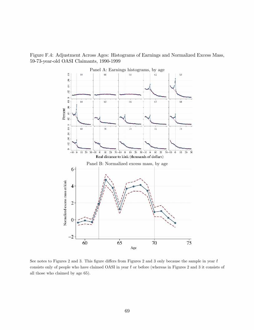
Figure F.4: Adjustment Across Ages: Histograms of Earnings and Normalized Excess Mass,59-73-year-old OASI Claimants, 1990-1999

Panel A: Earnings histograms, by age

Panel B: Normalized excess mass, by age

See notes to Figures 2 and 3. This figure differs from Figures 2 and 3 only because the sample in year tconsists only of people who have claimed OASI in year t or before (whereas in Figures 2 and 3 it consists ofall those who claimed by age 65).

69

Figure F.5: Adjustment Across Ages: Histograms of Earnings and Normalized Excess Mass,59-73-year-olds Claiming OASI by Age 65, 1972-1982

Panel A: Earnings histograms, by age

Panel B: Normalized excess mass, by age

See notes to Figures 2 and 3. This figure differs from Figures 2 and 3 only because the years examined are

1972-1982 (whereas in Figures 2 and 3 the years examined are 1990-1999).

70

Figure F.6: Adjustment Across Ages: Histograms of Earnings and Normalized Excess Mass,59-73-year-olds Claiming OASI by Age 65, 1983-1989

Panel A: Earnings histograms, by age

Panel B: Normalized excess mass, by age

See notes to Figures 2 and 3. This figure differs from Figures 2 and 3 only because the years examined are

1983-1989 (whereas in Figures 2 and 3 the years examined are 1990-1999).

71

Figure F.7: Adjustment Across Ages: Histograms of Earnings and Normalized Excess Mass,59-73-year-olds Claiming OASI by Age 65, 2000-2006

Panel A: Earnings histograms, by age

Panel B: Normalized excess mass, by age

See notes to Figures 2 and 3. This figure differs from Figures 2 and 3 only because the years examined are

2000-2006 (whereas in Figures 2 and 3 the years examined are 1990-1999). As explained in the main text,

the NRA slowly rose from 65 for cohorts that reached age 62 during this period; the results are extremely

similar when the sample is restricted to those who claimed by 66, instead of 65. In the year of attaining

NRA, the AET applies for months prior to such attainment.

72

Figure F.8: Comparison of Normalized Excess Bunching Among 62-64 Year-Olds and 66-69Year-Olds, 1982-2004

Note: the figure shows excess normalized bunching among 62-64 year-olds and 66-69 year-olds in each year

from 1982 to 2004. Note the caveat that the 62-64 year-old group faces a notch at the exempt amount, as

opposed to the kink faced by those 66-69.

73

Figure F.9: Adjustment Across Ages: Histograms of Earnings, 66-69 Year-Olds, 1999-2001

Panel A: Earnings histogram, 66-69 year-olds, 1999

Panel B: Earnings histogram, 66-69 year-olds, 2000

Panel C: Earnings histogram, 66-69 year-olds, 2001

Note: the figure shows a histogram of earnings in 1999, 2000, and 2001, using LEHD data on 66-69

year-olds. Earnings are measured relative to the kink, shown at zero.

74

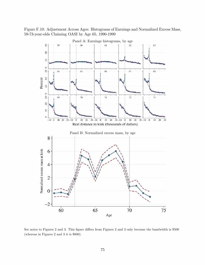
Figure F.10: Adjustment Across Ages: Histograms of Earnings and Normalized Excess Mass,59-73-year-olds Claiming OASI by Age 65, 1990-1999

Panel A: Earnings histograms, by age

Panel B: Normalized excess mass, by age

See notes to Figures 2 and 3. This figure differs from Figures 2 and 3 only because the bandwidth is $500

(whereas in Figures 2 and 3 it is $800).

75

Figure F.11: Robustness to Polynomial Degree: Normalized Excess Mass by Age and Year,OASI Claimants by 65

Panel A: Normalized Excess Mass by Age, 1990-1999

Panel B: Normalized Excess Mass by Year, Ages 66-69

Notes: The figure shows the difference in estimates of normalized excess bunching as we vary the degree of

the polynomial used. For additional notes on the samples see Figure 3 for Panel A and Figure 4 for Panel B.

76

Figure F.12: Robustness to the Excluded Region: Normalized Excess Mass by Age and Year,OASI Claimants by 65

Panel A: Normalized Excess Mass by Age, 1990-1999

Panel B: Normalized Excess Mass by Year, Ages 66-69

Notes: The figure shows the difference in estimates of normalized excess bunching as we vary the region

about the kink that is "dummied out" in the polynomial estimation. For additional notes on the samples

see Figure 3 for Panel A and Figure 4 for Panel B.

77

Figure F.13: Adjustment by Sex: Histograms of Earnings, 59-73-year-olds Claiming OASIby Age 65, 1990-1999

See notes to Figure 2. The sample examined is the same as in Figure 2 but examines men and women

separately.

78

Figure F.14: Adjustment Across Ages: Histograms of Earnings, 59-73-year-olds ClaimingOASI by Age 65 with Self-Employment Income, 1990-1999

See notes to Figure 2. The figure differs from Figure 2 only because the sample consists of those with

positive self-employment income (whereas in Figure 2 those with positive self-employment income are

excluded).

79

Figure F.15: Mean Percentage Change in Earnings from Age 69 to 70, by Earnings at 69,1990-1998

Note: The figure shows the mean percentage change in earnings from age 69 to age 70 (y-axis), against

earnings at age 69 (x-axis). Earnings are measured relative to the kink, shown at zero on the x-axis. The

data are a 20 percent random sample of 69-year-olds in the LEHD in 1990-1998. We exclude 1999 as a base

year in this and similar graphs because the AET is eliminated for those over NRA in 2000.

80

Figure F.16: Probability that Earnings Move with Kink, 1990-1998

Note: The figure shows the probabiliy that individual earnings move with the kink from year to year (i.e.

the probability that an individual locates at the kink in year t+ 1, conditional on locating at the kink inyear t), for age groups 58 to 60, 62 to 63, and 65 to 68. (Each of these ages refers to age in year t.) Resultsare similar when considering similar age bins. The kink is defined as the region within $2800 of the exempt

amount. We exclude the year 1999 because the AET is eliminated for those over NRA in 2000. See other

notes to Figure 2.

81

Figure F.17: Earnings Distributions by Age, OASI Claimants by Age 65, 1990-1999

Panel A: Earnings Distributions by Age, 60-62

Panel B: Earnings Distributions by Age, 69-71

Notes: The figure shows earnings distributions at ages 60, 61, and 62 (Panel A) and at ages 69, 70, and 71

(Panel B).

82

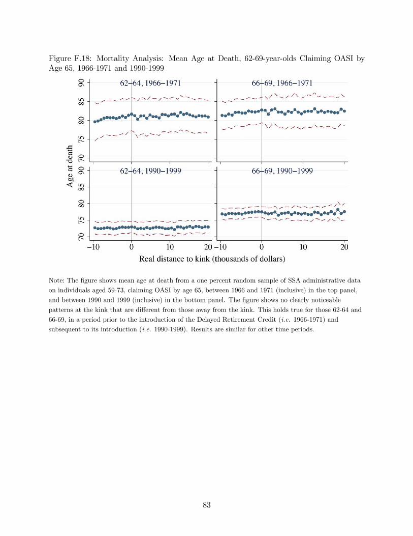
Figure F.18: Mortality Analysis: Mean Age at Death, 62-69-year-olds Claiming OASI byAge 65, 1966-1971 and 1990-1999

Note: The figure shows mean age at death from a one percent random sample of SSA administrative data

on individuals aged 59-73, claiming OASI by age 65, between 1966 and 1971 (inclusive) in the top panel,

and between 1990 and 1999 (inclusive) in the bottom panel. The figure shows no clearly noticeable

patterns at the kink that are different from those away from the kink. This holds true for those 62-64 and

66-69, in a period prior to the introduction of the Delayed Retirement Credit (i.e. 1966-1971) and

subsequent to its introduction (i.e. 1990-1999). Results are similar for other time periods.

83

Figure F.19: Normalized Excess Mass at Kink by Age, 1966-1971

Note: The figure shows normalized excess bunching, ages 18 to 75, 1966-1971. We group ages into

three-year bins. See other notes to Figure 3.

84

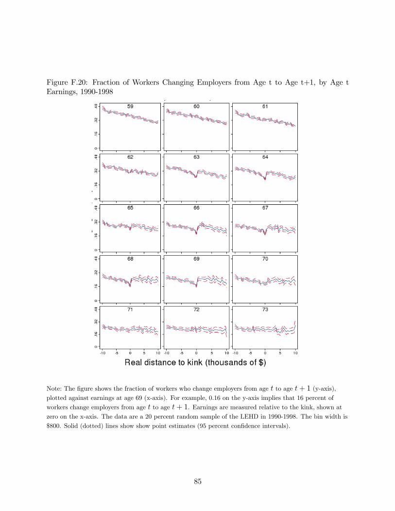
Figure F.20: Fraction of Workers Changing Employers from Age t to Age t+1, by Age tEarnings, 1990-1998

Note: The figure shows the fraction of workers who change employers from age t to age t+ 1 (y-axis),plotted against earnings at age 69 (x-axis). For example, 0.16 on the y-axis implies that 16 percent of

workers change employers from age t to age t+ 1. Earnings are measured relative to the kink, shown atzero on the x-axis. The data are a 20 percent random sample of the LEHD in 1990-1998. The bin width is

$800. Solid (dotted) lines show show point estimates (95 percent confidence intervals).

85

Figure F.21: Elasticity Estimates by Year, Saez (2010) Method, 1982-1994

Note: The figure shows elasticities estimated using the Saez (2010) method, by year from 1982 to 1994,

among 67-68 year-old OASI claimants. We use our methods for estimating normalized excess bunching but

use Saez’(2010) formula to calculate elasticities, under a constant density. This method yields the

following formula:

ε =

[log

(b

z∗+ 1

)]/[log

(1− τ 0

1− τ 1

)]

86

Figure F.22: Probability of claiming OASI in year t+1 among 61-68 year-olds in year t whoare not claiming, 1990-1998

Note: The figure shows the probabiliy that an individual claims OASI in year t+ 1, conditional on notclaiming OASI in year t, for those ages 61-68 in year t from 1990-1998.

87

G Appendix: Additional Estimates of ε and φ

Table G.1: Estimates of Elasticity and Adjustment Cost Using Sharp Change Method andDisappearance of Kink at Age 70

(1) (2) (3)

ε φ ε|φ = 0, Age 69

Basic 0.28 89.93 0.25[0.25, 0.34]*** [25.51, 240.00]*** [0.22, 0.30]***

Lognormal 0.30 $87.19 0.27[0.26, 0.36]*** [31.88, 256.39]*** [0.23, 0.32]***

Benefit Enhancement 0.42 $58.01 0.38[0.37, 0.50]*** [16.70, 146.86]*** [0.33, 0.45]***

Excluding FICA 0.36 $83.01 0.33[0.31, 0.43]*** [23.79, 213.17]*** [0.28, 0.38]***

Bandwidth = $500 0.20 $17.05 0.26[0.22, 0.32]*** [0.69, 76.00]*** [0.16, 0.23]***

68-70 year-olds 0.30 $79.10 0.28[0.27, 0.35]*** [24.61, 189.34]*** [0.25, 0.32]***

Note: The table estimates elasticities and adjustment costs using the removal of the AET at age 70, using

data on 69-71 year-olds. We cannot estimate the constrained elasticity using only data on age 70 because

the benefit reduction rate is zero at that age. We show these results in the Appendix, rather than the main

text, because the estimates of excess bunching at age 70 are potentially affected by the coarse measure of

age that we use, as explained above in the Appendix. To address this issue, we use both age 70 and age 71

in estimating these results. Using only age 70– or alternatively using only age 71– both show very similar

results, which is unsurprising because Figure 3 shows that normalized excess bunching is similar at ages 70

and 71. The row labeled "68-70 year-olds" uses data from ages within this range. See also notes to Table 2.

88

Table G.2: Estimates of Elasticity and Adjustment Cost Using Sharp Change Method and1990 Policy Change, Assuming no Pre-Period Bunching Attenuation

(1) (2) (3) (4)

ε φ ε|φ = 0

1990 1989

Baseline 0.22 $139.53 0.39 0.22[0.18, 0.26]*** [46.25, 359.40]*** [0.33, 0.48]*** [0.18, 0.26]***

Lognormal density 0.24 $149.87 0.43 0.24[0.19, 0.29]*** [42.55, 426.32]*** [0.35, 0.54]*** [0.19, 0.29]***

Benefit Enhancement 0.37 $76.24 0.59 0.37[0.30, 0.43]*** [17.28, 237.63]*** [0.49, 0.73]*** [0.30, 0.43]***

Excluding FICA 0.30 $119.84 0.50 0.30[0.25, 0.35]*** [32.33, 344.45]*** [0.42, 0.62]*** [0.25, 0.35]***

Bandwidth = $500 0.24 $83.80 0.38 0.24[0.19, 0.30]*** [5.86, 296.54]*** [0.30, 0.50]*** [0.19, 0.30]***

68-70 year-olds 0.31 $106.32 0.50 0.31[0.27, 0.34]*** [25.21, 291.94]*** [0.42, 0.62]*** [0.27, 0.34]***

Note: The table applies the Sharp Change method to the 1990 policy change, using data from 1989 and

1990, but assumes that bunching in 1989 is not attenuated by adjustment frictions. The constrained

estimate of bunching using data only from 1989 is mechanically the same as the unconstrained estimate, as

both rely on the Saez (2010) formula for bunching. See also notes to Appendix Table G.1.

89

Table G.3: Estimates of Elasticity and Adjustment Cost Using Sharp Change Method andElimination of Earnings Test in 2000 for 66-69 Year-Olds

(1) (2) (3)

ε φ ε|φ = 0, 1999

Baseline 0.10 $23.23 0.09[0.03, 0.19]*** [0.00, 331.52]* [0.04, 0.14]***

Lognormal density 0.10 $20.17 0.09[0.03, 0.21]*** [0.00, 346.90]* [0.04, 0.14]***

Benefit Enhancement 0.15 $14.93 0.14[0.04, 0.36]*** [0.00, 350.46]* [0.07, 0.21]***

Excluding FICA 0.13 $21.31 0.12[0.03, 0.28]*** [0.00, 402.69]* [0.06, 0.18]***

Bandwidth = $500 0.10 $56.48 0.09[0.07, 0.21]*** [0.03, 367.05]** [0.05, 0.13]***

1998 to 2000 0.12 $23.09 0.11[0.08, 0.55]*** [0.00, 957.13]* [0.07, 0]***

Note: The table applies the Sharp Change method to the 2000 policy change, using data on 1999 and 2000.

It is not possible to perform the constrained estimate using a cross-section from the year 2000 because the

marginal tax rate is zero in this year, implying that the elasticity is undefined. The final row uses data

from 1998 and 2000, rather than 1999 and 2000. Note that the left endpoint of the confidence interval is

sometimes at 0.00 even though the p-value indicates significance at the 5 percent level; this is because a

few of the bootstrap replications show point estimates that are positive and very small so round to 0.00.

See also notes to Appendix Table G.1.

90

Table G.4: Estimates of Elasticity and Adjustment Cost Using Comparative Static Methodand 1990 Policy Change

(1) (2) (3) (4)

ε φ ε|φ = 0

1993 1989

Baseline 0.21 $0.00 0.21 0.21[0.18, 0.34]*** [0.00, 902.56] [0.14, 0.31]*** [0.17, 0.26]***

Lognormal density 0.24 $33.35 0.22 0.23[0.20, 0.36]*** [0.00, 577.01] [0.15, 0.34]*** [0.19, 0.29]***

Benefit Enhancement 0.37 $78.09 0.32 0.36[0.30, 0.50]*** [0.00, 352.03] [0.21, 0.47]*** [0.29, 0.43]***

Excluding FICA 0.30 $58.54 0.27 0.29[0.25, 0.42]*** [0.00, 492.47] [0.18, 0.40]*** [0.24, 0.35]***

Bandwidth = $500 0.25 $0.00 0.25 0.25[0.21, 0.80]*** [0.00, 4188.55] [0.20, 0.35]*** [0.19, 0.32]***

1988 and 1993 0.26 $146.33 0.21 0.25[0.23, 0.33]*** [0.00, 408.86] [0.14, 0.31]*** [0.22, 0.28]***

Linear Approximation 0.46 $379.10 0.30 0.39[0.58, 0.60]*** [351.27, 406.93]*** [0.19, 0.41]*** [0.31, 0.47]***

Note: The table applies the Comparative Static method to the 1990 policy change, using data from 1989

and 1993. "Linear approximation" refers to estimates based on the linearized formulas presented in the

text. See also notes to Appendix Table G.1.

91