Embed Size (px)
Citation preview

Financial Frictions, Investment and Tobin’s q∗
Guido Lorenzoni†
MIT and NBERKarl Walentin‡
Sveriges Riksbank
October 28, 2007
Abstract
We develop a model of investment with financial constraints and use it to investigate
the relation between investment and Tobin’s q. A firm is financed partly by insiders, who
control its assets, and partly by outside investors. When their wealth is scarce, insiders
earn a rate of return higher than the market rate of return, i.e., they receive a quasi-rent
on invested capital. This rent is priced into the value of the firm, so Tobin’s q is driven
by two forces: changes in the value of invested capital, and changes in the value of the
insiders’ future rents per unit of capital. This weakens the correlation between q and
investment, relative to the frictionless benchmark. We present a calibrated version of
the model, which, due to this effect, generates realistic correlations between investment,
q, and cash flow.
Keywords: Financial constraints, optimal financial contracts, investment, Tobin’s q,
limited enforcement.
JEL codes: E22, E30, E44, G30.
∗We thank for useful comments Andrew Abel, Daron Acemoglu, João Ejarque, Mark Gertler, VeronicaGuerrieri, Hubert Kempf, Sydney Ludvigson, Martin Schneider, and seminar participants at New YorkUniversity, MIT, University of Oslo, EEA Meetings (Amsterdam), Minneapolis FED, Sveriges Riksbank,Uppsala University, Norges Bank, SED Meetings (Vancouver), NBER Summer Institute 2006, and CEPR-Bank of Finland conference on Credit and the Macroeconomy. The views expressed in this paper are thoseof the authors and not necessarily those of the Executive Board of Sveriges Riksbank.
†E-mail: [email protected].‡E-mail: [email protected].

1 Introduction
The standard model of investment with convex adjustment costs predicts that movements in
the investment rate should be entirely explained by changes in Tobin’s q. This prediction has
generally been rejected in empirical studies, which show that cash flow and other measures
of current profitability have a strong predictive power for investment, after controlling for q.
These results have been interpreted as evidence of financial frictions which make investment
more sensitive to internal sources of finance, for which cash-flow is a natural proxy, than to
expected profitability, captured by q. Starting with Fazzari, Hubbard, and Petersen (1988),
this interpretation has been pursued and developed by a vast empirical literature.1 At the
same time, a literature which goes back to Bernanke and Gertler (1989), Carlstrom and
Fuerst (1997), Kiyotaki and Moore (1997), and Bernanke, Gertler and Gilchrist (2000),
has developed models of investment with financial constraints which are incorporated into
full dynamic general equilibrium models and used to study the aggregate implications of
financial frictions.2 These models capture the financial constraint by focusing on some
basic informational or enforcement friction which affects the agents who run the firms in
the economy. In this paper, we study the implications of a model of this type for the q
theory of investment. That is, we ask whether a simple microfounded model of financial
frictions can deliver realistic correlations between investment, q, and cash-flow. This exercise
provides a basic test of consistency for this class of models.
We start from a setup with firms controlled by “insiders,” who can be interpreted as
the entrepreneur, the manager, or the controlling shareholder. We assume that the insider
has the ability to partially divert the assets of the firm and, if he does so, he is punished
by losing control of the firm. In this setup, we characterize the optimal long-term financial
contract between the insider and the outside investors.
Aside from the enforcement friction, our model is virtually identical to the classic
Hayashi (1982) model. In particular, it features convex adjustment costs and constant
returns to scale. This allows us to identify in a clean way the effect of the financial friction
on the equilibrium behavior of investment and q. As in Hayashi (1982), we make a distinc-
tion between marginal q, which captures the marginal value of new investment, and average
q, which is the ratio of the total value of the firm to the replacement value of its capital
stock. Average q is observable and, thus, is the notion of q typically used in empirical
studies.
On the analytical side, we show that the financial constraint introduces a positive wedge
between marginal q and average q. The wedge between average and marginal q reflects the
tension between the future profitability of investment and the availability of internal funds
in the short run. On the quantitative side, we use a calibrated version of the model to
1See Hubbard (1998) for a survey and references below.2A non-exhaustive list of recent applications of “financial accelerator” models includes Christiano, Motto,
and Rostagno (2003), Iacoviello (2005), Gertler, Gilchrist, and Natalucci (2007), Faia and Monacelli (2007).
1
show that this wedge varies over time, breaking the one-to-one correspondence between
investment and average q which holds in the frictionless model. We then simulate the
model and run standard investment regressions on the simulated data. From this exercise
we obtain coefficients on q and cash flow which are in line with those found in empirical
regressions. We conclude that our simple model is able to replicate the basic correlation
patterns between investment, asset prices, and cash-flow.
To assess the role of the financial friction, we compare the quantitative implications
of our model with those of the frictionless benchmark. In the frictionless benchmark, the
coefficient on q in the investment regression is equal to the inverse of the coefficient on
the quadratic term in the adjustment cost function. The presence of the financial friction
reduces this coefficient by a factor of six while, at the same time, generating a large positive
coefficient on cash flow.
A growing number of papers uses recursive methods to characterize optimal dynamic
financial contracts in environments with different forms of contractual frictions (DeMarzo
and Fishman, 2003, Quadrini, 2004, Clementi and Hopenhayn, 2006, DeMarzo and San-
nikov, 2006, and Atkeson and Cole, 2005). The limited enforcement friction in this paper
makes it closer to the models in Albuquerque and Hopenhayn (2004) and Cooley, Marimon
and Quadrini (2004). Within this literature, Biais, Mariotti, Plantin and Rochet (2007)
look more closely at the implications of the theory for asset pricing. In particular, they
find a set of securities that implements the optimal contract and then study the stochastic
behavior of the prices of these securities. Here, our objective is to examine the model’s
implication for q theory, therefore we simply focus on the total value of the firm, which
includes the value of all the claims held by insiders and outsiders. A distinctive feature of
our approach is that we make heavy use of the assumption of constant returns to scale, so
that optimal contracts take a simple linear form. This makes aggregation straightforward
and makes our model very easy to incorporate into a general equilibrium environment. In
this sense, the model retains the simplicity of a representative agent model, while allowing
for rich dynamics of net worth, profits and investment.
The idea of looking at the statistical implications of a simulated model to understand
the empirical correlation between investment and q goes back to Sargent (1980). Recently,
Gomes (2001), Cooper and Ejarque (2001, 2003) and Abel and Eberly (2004, 2005) have
followed this route, introducing both financial frictions and decreasing returns and market
power to match the existing empirical evidence.3 The conclusion one can derive from
this set of papers is that decreasing returns and market power help to generate realistic
correlations, while financial frictions do not. In particular, Gomes (2001) and Cooper
and Ejarque (2003) obtain negative results which stand in contrast to the results obtained
here. In their simulated economies with financial frictions Tobin’s q still explains most of
3See Schiantarelli and Georgoutsos (1990) for an early study of q theory in a model where firms havemarket power.
2

the variability in investment, and cash flow does not provide any additional explanatory
power.4 The main difference between our approach and their approach is the modeling of
the financial constraint. They introduce a constraint on the flow of outside finance that can
be issued each period. Here instead, we explicitly model a contractual imperfection and
solve for the optimal long-term contract. This adds a state variable to the problem, namely
the stock of existing liabilities of the firm, thus generating slow-moving dynamics in the gap
between internal funds and the desired level of investment. These dynamics account for
the empirical disconnect between investment and q and explain why our model of financial
frictions is better able to replicate observed correlations. On the other hand, there are some
parallels between our approach and the approach based on decreasing returns and market
power, in particular with the “growth options” mechanism emphasized in Abel and Eberly
(2005). Both approaches imply that movements in q can reflect changes in future rents that
are unrelated to current investment. In our paper these rents are not due to market power,
but to the scarcity of entrepreneurial wealth, which evolves endogenously.
Following Fazzari, Hubbard and Petersen (1988) there has been a large empirical liter-
ature exploring the relation between investment and q using firm level data. The majority
of these papers find small coefficients on q and positive and significant coefficients on cash
flow and other variables describing the current financial condition of a firm. This result has
been ascribed to measurement error in q, possibly caused by non-fundamental stock market
movements.5 Measurement error would reduce the explanatory power of q, and cash flow
would then appear as significant, given that it is a good predictor of future profits. Gilchrist
and Himmelberg (1995) show that this is insufficient to explain the failure of q theory in
investment regressions.6 They replace the value of q obtained by financial market prices
with a measure of “fundamental q” (which employs current cash flow as a predictor of future
profits), and they show that current cash flow retains its independent explanatory power.
Finally, Hennessy and Whited (2007) build a rich structural model of firms’ investment with
financial frictions, which is then estimated by simulated method of moments on firm-level
data. They find that the financial constraint plays an important role in explaining observed
firms’ behavior.7 The evidence in this literature provides the starting motivation for our
exercise. In an extension of the model (Section 4) we introduce firm-level heterogeneity and
further explore the connection between our model and panel data evidence.
The paper is organized as follows. Section 2 presents the model, the derivation of the4See also Moyen (2004).5The debate is open whether non-fundamental movements in q should affect investment or not. See
Chirinko and Schaller (2001), Gilchrist, Himmelberg and Huberman (2005) and Panageas (2005).6See Erickson and Whited (2000) and Bond and Cummins (2001) for a contrarian view. See Rauh (2006)
for recent evidence in favor of the financial frictions interpretation.7 In their model, due to the complexity of the estimation task, the financial friction is introduced in a
relatively “reduced form,” by assuming that there are some transaction costs associated to the issuance ofnew equity or new debt, as in Cooper and Ejarque (2003) and Gomes (2001). The difference in results,relative to these papers, appears due to the fact that Hennessy and Whited (2007) also match the behaviorof a number of financial variables.
3

optimal contract, and the equilibrium analysis. Section 3 contains the calibration and
simulation results. In Section 4 we extend the model to allow for firm-level heterogeneity.
Section 5 concludes. All proofs not in the text are in the appendix.
2 The Model
2.1 The environment
Consider an economy populated by two groups of agents of equal mass, consumers and
entrepreneurs. Consumers are infinitely lived and have a fixed endowment of labor lC , which
they supply inelastically on the labor market at the wage wt. Consumers are risk neutral
and have a discount factor βC . Entrepreneurs have finite lives, with a constant probability
of death γ. Each period, a fraction γ of entrepreneurs is replaced by an equal mass of newly
born entrepreneurs. Entrepreneurs begin life with no capital and have a labor endowment
lE in the first period of life, which gives them an initial wealth wtlE. Entrepreneurs are
also risk neutral, with a discount factor βE < βC . The last assumption, together with the
assumption of finitely lived entrepreneurs, is needed to ensure the existence of a steady
state with a binding financial constraint. We normalize total labor supply to one, that is,
lC + γlE = 1.
Starting in their second period of life, entrepreneurs have access to the constant-returns-
to-scale technology AtF (kt, lt), where kt is the stock of capital installed in period t−1, andlt is labor hired on the labor market. The productivity At is equal across entrepreneurs and
follows the stationary stochastic process At = Γ (At−1, t), where t is an i.i.d. shock drawn
from the discrete p.d.f. π ( t). We normalize the unconditional mean of At to 1.
Investment in new capital is subject to convex adjustment costs, which we now describe.
At the end of each period, after production has taken place, capital depreciates and the
entrepreneur has access to kt units of used capital. Then, he can trade capital on the used
capital market, at the price qot , and choose to hold on to kot units of used capital, where k
ot
may be different from kt. Next, the entrepreneur chooses the capital stock for next period
kt+1, and pays G (kt+1, kot ), which includes both the cost of acquiring new capital and the
installation (or uninstallation) costs. The function G (kt+1, kot ) is increasing and convex in
kt+1, decreasing in kot , homogeneous of degree one, and satisfies ∂G (kt+1, kot ) /∂kt+1 = 1 if
kt+1 = kot .
An entrepreneur born at date t0 finances his current and future investment by issuing a
long-term financial contract, specifying a sequence of state-contingent transfers (which can
be positive or negative) from the entrepreneur to the outside investors, {dt}∞t=t0 . In periodt = t0, his budget constraint is
cEt +G (kt+1, kot ) + qot k
ot ≤ wtlE − dt.
4
The entrepreneur uses his initial wealth to consume and to acquire used capital and trans-
form it into capital ready for use in t0 + 1. Furthermore, he can increase his consumption
and investment by borrowing from consumers, i.e., choosing a negative value for dt0 . In the
remaining periods, the budget constraint is
cEt +G (kt+1, kot ) + qot (k
ot − kt) ≤ AtF (kt, lt)−wtlt − dt.
He uses current revenues, net of labor costs and financial payments, to finance consumption
and investment. At the beginning of each period t, the entrepreneur learns whether that is
his last period of activity. Therefore, in the last period, he liquidates all the capital kt and
consumes the receipts, setting
cEt = AtF (kt, lt)− wtlt + qot kt − dt.
From then on, the payments dt are set to zero.
Financial contracts are subject to limited enforcement. The entrepreneur controls the
firm’s assets kt and can, in each period, run away, diverting a fraction (1− θ) of them. If
he does so, he re-enters the financial market as if he was a young entrepreneur, with initial
wealth given by the value of the diverted assets, and zero liabilities. That is, the only
punishment for a defaulting entrepreneur is the loss of a fraction θ of the firm’s assets.8
Aside from limited enforcement no other imperfections are present, in particular, financial
contracts are allowed to be fully state-contingent.
2.2 Recursive competitive equilibrium
We will focus our attention on recursive equilibria where the economy’s dynamics are fully
characterized by the vector of aggregate state variables Xt ≡ (At,Kt, Bt), where Kt is
the aggregate capital stock and Bt denotes the aggregate liabilities of the entrepreneurs,
to be defined in a moment. In the equilibria considered, consumers always have positive
consumption. Therefore, the market discount factor is equal to their discount factor, βC ,
and the net present value of the liabilities of an individual entrepreneur can be written as
bt = Et
" ∞Xs=0
βsCdt+s
#.
The variable Bt is equal to the economy-wide aggregate of these liabilities.
A recursive competitive equilibrium is defined by law of motions for the endogenous
8Here, we just take this as an institutional assumption. For a microfoundation, we could assume thatdefaulting entrepreneurs are indistinguishable from young entrepreneurs. However, this would require ad-dressing a number of informational issues, which would considerably complicate the analysis.
5
state variables:
Kt = K (Xt−1) ,
Bt = B (Xt−1, t) ,
and by two maps, w (Xt) and qo (Xt), which give the market prices as a function of the
current state. Given these four objects, we can derive the optimal individual behavior
of the entrepreneurs. The quadruple K,B, w (.) and qo (.) forms a recursive competitive
equilibrium if: (i) the entrepreneurs’ optimal behavior is consistent with the law of motions
K and B, and (ii) the labor and used capital market clear. In the next two subsections, wefirst characterize entrepreneurs’ decisions, and then aggregate and check market clearing.
We use
Xt = H (Xt−1, t) ,
to denote in a compact way the law of motion for Xt derived from the laws of motion
Γ,K, and B.
2.3 Optimal financial contracts
Let us consider first the optimization problem of the individual entrepreneur. Exploiting
the assumption of constant returns to scale, we will show that the individual problem is
linear. This property will greatly simplify aggregation.
We describe the problem in recursive form, dropping time subscripts. Consider a contin-
uing entrepreneur, in stateX, who controls a firm with capital k and outstanding liabilities b.
Let V (k, b,X) denote his end-of-period expected utility, computed after production takes
place and assuming that the entrepreneur chooses not to default in the current period. The
entrepreneur takes as given the law of motion for the aggregate state X and the pricing
functions w (X) and qo (X).
The budget constraint takes the form
cE +G¡k0, ko
¢+ qo (X) ko ≤ AF (k, l)− w (X) l + qo (X) k − d.
Lemma 1 allows us to rewrite it as
cE + qm (X) k0 ≤ R (X) k − d, (1)
where qm (X) is the shadow price of the new capital k0, and R (X) is the (gross) return perunit of capital, on the installed capital k.
Lemma 1 Given the prices w (X) and qo (X), there are two functions qm (X) and R (X)
6
that satisfy the following conditions for any k0 and k,
qm (X) k0 = minko
©G¡k0, ko
¢+ qo (X) ko
ª,
R (X) k = maxl{AF (k, l)− w (X) l}+ qo (X) k.
This lemma exploits the assumption of constant returns to show that qm (X) and R (X)
are independent of the current and future capital stocks, k and k0, and only depend on theprices w (X) and qo (X). The variable qm (X) is equal to marginal q in our model, and will
be discussed in detail below.
A continuing entrepreneur can satisfy his existing liabilities b either by repaying now
or by promising future repayments. Let b0 ( 0) denote next-period liabilities, contingent onthe realization of the aggregate shock 0, if tomorrow is not a terminal date, and let b0L (
0)denote the same, in the event of termination. Then, the entrepreneur faces the constraint
b = d+ βC¡(1− γ)E[b0
¡ 0¢] + γE[b0L¡ 0¢]¢ , (2)
where the expectation is taken with respect to 0.The entrepreneur has to ensure that his future promised repayments are credible. Recall
that, if the entrepreneur defaults, his liabilities are set to zero and he has access to a
fraction (1− θ) of the capital. Therefore, if tomorrow is a continuation date, his promised
repayments b0 ( 0) have to satisfy the no-default condition
V (k0, b0¡ 0¢ ,X 0) ≥ V ((1− θ) k0, 0,X 0) (3)
for all 0. Throughout this section, X 0 stands for H (X, 0). If tomorrow is the final period,the entrepreneur can either liquidate his firm, getting R (X 0) k0, and repay his liabilities,or default and get (1− θ)R (X 0) k0. Therefore, the no-default condition in the final periodtakes the form
R¡X 0¢ k0 − b0L
¡ 0¢ ≥ (1− θ)R¡X 0¢ k0, (4)
which again needs to hold for all 0.We are now ready to write the Bellman equation for the entrepreneur:
V (k, b,X) = maxcE ,k0,b0(.),b0L(.)
cE + βE (1− γ)E£V¡k0, b0
¡ 0¢ ,X 0¢¤++βEγE
£R¡X 0¢ k0 − b0L
¡ 0¢¤ (P )
s.t. (1), (2), (3) and (4).
Notice that, except for constraint (3), all constraints are linear in the individual states
k and b, and in the choice variables cE, k0, b0 (.) and b0L (.). Let us make the conjecture that
7

the value function is linear and takes the form
V (k, b,X) = φ (X) (R (X) k − b) , (5)
for some positive, state-contingent function φ (X). Then, the no-default condition (3) be-
comes linear as well, and can be rewritten as
b0¡ 0¢ ≤ θR
¡X 0¢ k0. (3’)
This is a form of “collateral constraint,” which implies that an entrepreneur can only pledge
a fraction θ of the future gross returns R (X 0) k.9 The crucial difference with similar con-straints in the literature (e.g., in Kiyotaki and Moore (1997)), is the fact that we allow for
fully state-contingent securities.
Before stating Proposition 3, we impose some restrictions on the equilibrium prices w (.)
and qo (.) and on the law of motion H. These conditions ensure that the entrepreneur’s
problem is well defined and deliver a simple optimal contract where the collateral constraint
(3’) is always binding. In subsection 2.4 we will verify that these conditions are met in
equilibrium.
Suppose the law of motion H admits an ergodic distribution for the aggregate state X,
with support X. Assume that equilibrium prices are such that the following inequalities
hold for each X ∈ X:
βEE£R¡X 0¢¤ > qm (X) , (6)
θβCE£R¡X 0¢¤ < qm (X) , (7)
and(1− γ) (1− θ)E [R (X 0)]qm (X)− θβCE [R (X 0)]
< 1. (8)
Condition (6) implies that the expected rate of return on capital E [R (X 0)] /qm (X) is greaterthan the inverse discount factor of the entrepreneur, so a continuing entrepreneur prefers
investment to consumption. Condition (7) implies that “pledgeable” returns are insufficient
to finance the purchase of one unit of capital, i.e., investment cannot be fully financed
with outside funds. This condition ensures that investment is finite. Finally, condition (8)
ensures that the entrepreneur’s utility is bounded.
Before introducing one last condition, we need to define a function φ, which summarizes
information about current and future prices.
Lemma 2 When conditions (6)-(8) hold, there exists a unique function φ : X → [1,∞)9Constraint (4) immediately gives an analogous inequality for b0L.
8

that satisfies the following recursive definition
φ (X) =βE (1− θ)E [(γ + (1− γ)φ (X 0))R (X 0)]
qm (X)− θβCE [R (X 0)]. (9)
This function satisfies φ (X) > 1 for all X ∈ X.
A further condition on equilibrium prices is then:
φ (X) >βEβC
φ¡X 0¢ (10)
for all X ∈ X and all X 0 = H (X, 0). Condition (10) ensures that entrepreneurs never delayinvestment. Namely, it implies that they always prefer to invest in physical capital today
rather than buying a state-contingent security that pays in some future state.
The function φ defined in Lemma 2 will play a central role in the rest of the analysis.
The next proposition shows that substituting φ (X) on the right-hand side of (5), gives us
the value function for the entrepreneur (justifying our slight abuse of notation). Define the
net worth of the entrepreneur
n (k, b,X) ≡ R (X) k − b,
which represents the difference between the liquidation value of the firm and the value of
its liabilities. Equation (5) implies that expected utility is a linear function of net worth
and φ (X) represents the marginal value of entrepreneurial net worth. We will go back to
its interpretation in subsection 2.5.
Proposition 3 Suppose the aggregate law of motion H and the equilibrium prices w (.) and
qo (.) are such that (6)-(8) and (10) hold, where φ (.) is defined as in Lemma 2. Then, the
value function V (k, b,X) takes the form (5) and the entrepreneur’s optimal policy is
cE = 0,
k0 =R (X) k − b
qm (X)− θβCE [R (X 0)], (11)
b0¡ 0¢ = b0L
¡ 0¢ = θR¡X 0¢ k0. (12)
The entrepreneur’s problem can be analyzed under weaker versions of conditions (6)-
(8) and (10). However, as we shall see in a moment, these conditions are appropriate for
studying small stochastic fluctuations around a steady state where the financial constraint
is binding.
9

2.4 Aggregation
Having characterized optimal individual behavior, we now aggregate and impose market
clearing on the labor market and on the used capital market. To help the reading of the
dynamics, we now revert to using time subscripts.
Each period, a fraction γ of entrepreneurs begins life with zero capital and labor income
wtlE. Their net worth is simply equal to their labor income. Moreover, a fraction (1− γ)
of continuing entrepreneurs has net worth equal to nt = Rtkt− bt. The aggregate net worthof the entrepreneurial sector, excluding entrepreneurs in the last period of activity, is then
given by
Nt = (1− γ) (RtKt −Bt) + γwtlE.
Using the optimal individual rules (11) and (12), we get the following dynamics for the
aggregate states Kt and Bt
Kt+1 =(1− γ) (RtKt −Bt) + γwtlE
qmt − θβCEt [Rt+1], (13)
Bt+1 = βCθRt+1Kt+1. (14)
Finally, the following conditions ensure that the prices wt and qot are consistent with market
clearing in the labor market and in the used capital market
wt = At∂F (Kt, 1)
∂Lt, (15)
qot = −∂G (Kt+1,Kt)
∂Kt. (16)
To clarify the role of condition (16), notice that all continuing entrepreneurs choose the same
ratio kot /kt+1, and this ratio must satisfy the first-order condition qot+∂G (kt+1, k
ot ) /∂k
ot = 0.
Market clearing on the used capital market requires that continuing entrepreneurs acquire all
the existing used capital stock, so Kt/Kt+1 is equal to kot /kt+1. This gives us condition (16).
Summing up, we have found a recursive equilibrium if the laws of motion K and B andthe pricing rules for wt and qot satisfy (13) to (16), and if they are such that conditions
(6)-(10) are satisfied. The next proposition shows that an equilibrium with these properties
exists under some parametric assumptions. Let the production function and the adjustment
cost function be:
AtF (kt, lt) = Atkαt l1−αt , (17)
G (kt+1, kt) = kt+1 − (1− δ) kt +ξ
2
(kt+1 − kt)2
kt. (18)
To construct a recursive equilibrium, we consider a deterministic version of the same econ-
omy (i.e., an economy where At is constant and equal to 1), and use the deterministic steady
10
state as a reference point. Let£A,A
¤be the support of At in the stochastic economy.
Proposition 4 Consider an economy with Cobb-Douglas technology and quadratic adjust-ment costs. Consider the steady-state equilibrium of the corresponding deterministic econ-
omy and suppose that it satisfies the following two properties: (i) the financial constraint
is binding at the steady state (βRSS > 1), (ii) the steady state is locally saddle-path stable.
Then there is a scalar ∆ > 0 such that, if A− A < ∆, there exists a recursive competitive
equilibrium of the stochastic economy with aggregate dynamics described by (13)-(14).
In the appendix we spell out conditions on the economy’s underlying parameters which
ensure that the deterministic steady state satisfies conditions (i) and (ii) in the hypothesis
of this proposition.10 These parametric restrictions are satisfied in all the calibrations
considered below.
Finally, as a useful benchmark, let us briefly characterize the frictionless equilibrium
which arises when θ = 1. In the frictionless benchmark, equilibrium dynamics are fully
characterized by the condition
qmt = βCEt [Rt+1] . (19)
The definitions of qmt and Rt are the same as those given in the constrained economy,
and so are the equilibrium conditions (15) and (16) for wt and qot . Given that βE < βC
entrepreneurs consume their wealth wtlE in the first period of their life and consume zero
in all future periods. Investment is entirely financed by consumers, which explains why the
consumers’ discount factor appears in the equilibrium condition (19).
2.5 Average q and marginal q
Having characterized equilibrium dynamics, we can now derive the appropriate expressions
for average q and for marginal q. Marginal q is immediately derived from the entrepreneur’s
problem as the shadow value of new capital, qmt . The definition of qmt in Lemma 1 and the
equilibrium condition (16) can be used to obtain
qmt =∂G (Kt+1/Kt, 1)
∂Kt+1.
This is the standard result in economies with convex adjustment costs: there is a one-to-one
relation between the investment rate and the shadow price of new capital.
To derive average q, we first need to obtain the financial value of a representative firm,
that is, the sum of the value of all the claims on the firm’s future earnings, held by insiders
(entrepreneurs) and outsiders (consumers). For firms in the last period of activity this value
is zero. For continuing firms, this gives us the expression
pt ≡ V (kt, bt,Xt) + bt − dt. (20)10See conditions (33) and (35) in the proof of Proposition 4.
11

We subtract the current payments to outsiders, dt, to obtain the end-of-period value of the
firm. Recall that continuing entrepreneurs receive zero payments in the optimal contract
(except in the final date), so there is no need to subtract current payments to insiders.
Dividing the financial value of the firm by the total capital invested we obtain average q
qt ≡ ptkt+1
.
Notice we divide by kt+1 because we are evaluating qt at the end of the period, after the
capital kt+1 has been installed. This is consistent with the fact that the value of the firm,
pt, is also evaluated at the end of the period. In the recursive equilibrium described above,
qt is the same for all continuing firms. For liquidating firms both pt and kt+1 are zero, so qtis not defined for those firms.
The next proposition shows that the financial constraint introduces a wedge between
marginal q and average q, and that the wedge is determined by φt, the marginal value of
entrepreneurial wealth.
Proposition 5 In the recursive equilibrium described in Proposition 4, average q is the
same for all continuing firms and is greater than marginal q, qt > qmt . Everything else
equal, the ratio qt/qmt is increasing in φt.
Proof. Substituting the value function in the value of the firm (20), and rearranging
gives
pt = (φt − 1) (Rtkt − bt) +Rtkt − dt. (21)
Using the entrepreneur’s budget constraint, constant returns to scale for G, and the equi-
librium properties of qot and qmt , gives
Rtkt − dt = G (kt+1, kot ) + qot k
ot =
=∂G (kt+1, k
ot )
∂kt+1kt+1 +
∂G (kt+1, kot )
∂kt+1kot + qot k
ot =
= qmt kt+1.
Substituting in (21) and rearranging gives
qt = (φt − 1)Rtkt − btkt+1
+ qmt . (22)
Notice that (11) implies that (Rtkt − bt) /kt+1 is equal across continuing firms. Given that
φt > 1 and bt ≤ θRtkt < Rtkt the stated results follow from this expression.
Notice that in the frictionless benchmark investment is fully financed by consumers and
we have bt = Rtkt, which immediately implies qt = qmt . In this case, the model boils down
to the Hayashi (1982) model: average q is identical to marginal q and is a sufficient statistic
for investment.
12

It is useful to provide some explanation for the wedge between average q and marginal q
in the constrained economy. First, notice that this wedge is not due to the difference in
the discount factors of entrepreneurs and consumers. In fact, if we evaluated the expected
present value of the entrepreneur’s payoffs {cEt+j} using the discount factor βC instead ofβE , we would get a quantity greater than V (kt, bt,Xt) and the measured wedge would be
larger.11 The fundamental reason why the wedge is positive is that φt > 1, the marginal
value of entrepreneurial wealth is larger than one. If φt was equal to 1, then the first term
on the right-hand side of (22) would be zero and the wedge would disappear.
To clarify the mechanism, consider an entrepreneur who begins life with one dollar
of wealth. Suppose he uses this wealth to start a firm financed only with inside funds
and consumes the receipts at date t + 1. The (shadow) price of a unit of capital is qmt ,
so the entrepreneur can install 1/qmt units of capital. In period t + 1 he receives and
consumes Rt+1/qmt . The value of the firm for the entrepreneur is then βEEt [Rt+1] /q
mt
which is greater than one, by condition (6). In short, the value of a unit of installed capital
is larger inside the firm than outside the firm, and this explains why q theory does not hold.
This discrepancy does not open an arbitrage opportunity, because the agents that can take
advantage of this opportunity (the entrepreneurs) are against a financial constraint. This
thought experiment captures the basic intuition behind Proposition 5.
To go one step further, notice that the entrepreneur can do better than following the
strategy described above. In particular, he can use borrowed funds on top of his own
funds, and he can re-invest the revenues made at t+1, rather than consume. The ability of
borrowing allows the entrepreneur to earn an expected leveraged return, between t and t+1,
equal to12
(1− θ)Et [Rt+1] / (qmt − θβCEt [Rt+1]) > Et [Rt+1] /q
mt .
Iterating expression (9) forward shows that φt is a geometric cumulate of future leveraged
returns discounted at the rate βE, taking into account the fact that, as long as the en-
trepreneur remains active, he can reinvest the returns made in his firm. Therefore, when
borrowing and reinvestment are taken into account, one dollar of wealth allows the entre-
preneur to obtain a value of φt > βEEt [Rt+1] /qmt > 1. At the same time, the entrepreneur
is receiving qmt kt+1 − 1 from outside investors (recall that he only has 1 dollar of internal
funds). Therefore, the value of the claims issued to outsiders must equal qmt kt+1−1. In con-clusion, an entrepreneur with one dollar to invest can start a firm valued at φt+qmt kt+1−1,which is larger than the value of invested capital, qmt kt+1, given that φt > 1.
11For the quantitative results presented in Section 3, we also experimented with this alternative definitionof q (discounting the entrepreneur’s claims at the rate βC instead of βE), with minimal effects on the results.12Notice that, from (11), 1// (qmt − θβCEt [Rt+1]) is the capital stock kt+1 which can be invested by an
entrepreneur with one dollar of wealth. In t + 1 the entrepreneur has to repay θRt+1kt+1 and can keep(1− θ)Rt+1kt+1. To prove the inequality, rearrange it and simplify to obtain
θβC (Et [Rt+1])2 > θqmt Et [Rt+1] .
The inequality follows from (a) and βC > βE .
13

3 Quantitative Implications
In this section, we examine the quantitative implications of the model looking at the joint
behavior of investment, Tobin’s q, and cash flow in a simulated economy. First, we give
a basic quantitative characterization of the economy’s response to a productivity shock.
Second, we ask whether the wedge between marginal q and average q in our model helps to
explain the empirical failure of q theory in investment regressions.
3.1 Baseline calibration
The production function is Cobb-Douglas and adjustment costs are quadratic, as specified
in (17) and (18). The productivity process is given by At = eat , where at follows the
autoregressive process
at = ρat−1 + t,
with t a Gaussian, i.i.d. shock.13
βC 0.97 βE 0.96
α 0.33 δ 0.05
ξ 8.5 ρ 0.75
θ 0.3 γ 0.06
lE 0.2
Table 1. Baseline calibration.
The baseline parameters for our calibration are reported in Table 1. The time period is a
year, so we set βC to give an interest rate of 3%. For the discount factor of the entrepreneurs,
we choose a value smaller but close to that of the consumers. The values for α and δ are
standard. The values of ξ and ρ are chosen to match basic features of firm-level data on
cash flow and investment. In particular, we consider the following statistics, obtained from
the Compustat dataset.14
r (CFK) σ (IK) σ (CFK)
0.51 0.061 0.128
where CFK denotes cash flow per unit of capital invested, IK denotes the investment
rate, r (.) denotes the (yearly) coefficient of serial correlation, and σ (.) the standard devia-13The theoretical analysis can be extended to the case where t is a continuous variable. To ensure that
At is bounded, we set At = A whenever eat < A and At = A whenever eat > A. As long as σ2 is small thebounds A and A are immaterial for the results.14We use the same data from Compustat as Gilchrist and Himmelberg (1995). The sample consists of 428
U.S. stock market listed firms from 1978 to 1989. We use the code of João Ejarque to calculate firm-specificstatistics separately for each variable. The moments reported in this paper are the means across all firms.Any ratio used (e.g. σ (IK) /σ (CFK)) is a ratio of such means.
14
tion. We calibrate ρ so that our simulated series replicate the autocorrelation of cash flow
r (CFK) = 0.51. In our baseline calibration this gives us ρ = 0.75. We set ξ to match
the ratio between cash flow volatility and investment volatility, σ (IK) /σ (CFK) = 0.48.
Given all the other parameters, this gives us ξ = 8.5.
Finally, the parameters θ, γ, and lE are chosen as follows. Fazzari, Hubbard and Petersen
(1988) report that 30% of manufacturing investment is financed externally. Based on this,
we choose θ = 0.3. The parameters γ and lE are chosen to obtain an outside finance premium
of 2%, as in Bernanke, Gertler and Gilchrist (2000). We experimented with different values
of γ and lE and found that, as long as the finance premium remains at 2%, the specific
choice of these two parameters has minimal effects on our results.
3.2 Impulse responses
In the model, the net investment rate of the representative firm is
IKt ≡ kt+1 − (1− δ) ktkt
,
and the ratio of cash flow to the firm’s capital stock is
CFKt ≡ AtF (kt, lt)− wtltkt
.
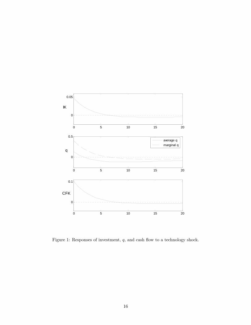
Figure 1 plots the responses of IKt, qt, and CFKt, following a positive technology shock.
All variables are expressed in terms of deviations from their steady-state values.
All three variables in Figure 1 increase on impact, as in the standard model without
financial frictions. However, the dynamics of average q are now jointly determined by
marginal q and by the wedge qt/qmt . Marginal q moves one for one with investment. Average
q initially rises with investment, but at some point (3 periods after the shock) it falls below
its steady-state value, while investment continues to be above the steady state for several
more periods (up to period 6 periods after the shock). As marginal q is reverting towards its
steady state the wedge remains large, thus pushing average q below the steady state. The
slow-moving dynamics of the wedge are responsible for breaking the synchronicity between
average q and investment.
In Proposition 5, we argued that the ratio of average q to marginal q is positively related
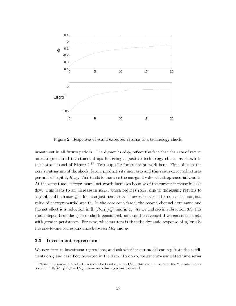
to φt, the marginal value of entrepreneurial net worth. The top panel of Figure 2 plots the
response of φt to the same technology shock, showing that φt decreases on impact following
the shock, and then slowly reverts to its steady-state value. The slow adjustment in the
wedge is closely related to the slow adjustment of φt.
To understand the response of φt, recall from the discussion in subsection 2.5 that the
dynamics of φt are closely related to those of the rate of return Et [Rt+1] /qmt , since φt
is a forward-looking measure which cumulates the discounted returns on entrepreneurial
15
0 5 10 15 20
0
0.05
IK
0 5 10 15 20
0
0.5
q
0 5 10 15 20
0
0.1
CFK
average qmarginal q
Figure 1: Responses of investment, q, and cash flow to a technology shock.
16
0 5 10 15 20-0.4
-0.3
-0.2
-0.1
0
0.1
φ
0 5 10 15 20
-0.05
0
E[R]/qm
Figure 2: Responses of φ and expected returns to a technology shock.
investment in all future periods. The dynamics of φt reflect the fact that the rate of return
on entrepreneurial investment drops following a positive technology shock, as shown in
the bottom panel of Figure 2.15 Two opposite forces are at work here. First, due to the
persistent nature of the shock, future productivity increases and this raises expected returns
per unit of capital, Rt+1. This tends to increase the marginal value of entrepreneurial wealth.
At the same time, entrepreneurs’ net worth increases because of the current increase in cash
flow. This leads to an increase in Kt+1, which reduces Rt+1, due to decreasing returns to
capital, and increases qmt , due to adjustment costs. These effects tend to reduce the marginal
value of entrepreneurial wealth. In the case considered, the second channel dominates and
the net effect is a reduction in Et [Rt+1] /qmt and in φt. As we will see in subsection 3.5, this
result depends of the type of shock considered, and can be reversed if we consider shocks
with greater persistence. For now, what matters is that the dynamic response of φt breaks
the one-to-one correspondence between IKt and qt.
3.3 Investment regressions
We now turn to investment regressions, and ask whether our model can replicate the coeffi-
cients on q and cash flow observed in the data. To do so, we generate simulated time series
15Since the market rate of return is constant and equal to 1/βC , this also implies that the “outside financepremium” Et [Rt+1] /q
mt − 1/βC decreases following a positive shock.
17

from our calibrated model and run the standard investment regression
IKt = a0 + a1qt + a2CFKt + et. (23)
The regression coefficients for the simulated model are presented in the first row of Table
2. As reference points, we report the coefficients that arise in the model without financial
frictions (θ = 1) and the empirical coefficients obtained by Gilchrist and Himmelberg (1995).
The latter are representative of the orders of magnitude obtained in empirical studies.
Absent financial frictions, q is a sufficient statistic for investment, so the model gives a
coefficient on cash flow equal to zero. In this case, the coefficient on q is equal to 1/ξ,
which, given the calibration above is equal to 0.118, a value substantially higher than those
obtained in empirical regressions. Adding financial frictions helps both to obtain a positive
coefficient on cash flow and a smaller coefficient on q. The impulse response functions
reported in Figure 1 help us to understand why. Financial frictions weaken the relation
between it and qt, while investment and cash flow remain closely related, due to the effect
of cash flow on entrepreneurial net worth.
a1 a2
Model with financial friction 0.018 0.444
Frictionless model 0.118 0.000
Gilchrist and Himmelberg (1995) 0.033 (0.016) 0.242 (0.038)
Table 2. Investment regressions.
Third line: Standard errors in parenthesis.
Notice that under the simple AR1 structure for productivity used here, a sizeable cor-
relation between q and investment is still present. Running a simple univariate regression
of investment on q gives a coefficient of 0.13, not too far from the frictionless coefficient,
and an R2 of 0.5. This is not surprising, given that only one shock is present. However,
once cash flow is added to the independent variables, the explanatory power of q falls dra-
matically. To see this, notice that the R2 of the bivariate regression is virtually 1, while
the R2 of a univariate regression of investment on cash flow alone is 0.995. So the additional
explanatory power of q is less than 1 percent of investment volatility.
The values of R2 just reported are clearly unrealistic and are a product of the simple
one-shock structure used. Furthermore, idiosyncratic uncertainty and measurement error
are absent from the exercise. For these reasons, we do not attempt to exactly replicate the
empirical coefficients for q and cash flow.16 Instead, our point here is that a reasonable
calibration of the model can help generate realistic coefficients for both q and cash flow, by
introducing a time-varying wedge between marginal q and average q. An extension of the
16By changing the model parameters, in particular increasing θ and ξ, it is possible to match exactly thecoefficients in Gilchrist and Himmelberg (1995).
18

model that allows for idiosyncratic uncertainty is discussed below.
3.4 Sensitivity
To verify the robustness of our result, we experiment with different parameter configura-
tions, in a neighborhood of the parameters introduced above. Table 3 shows the coefficients
of the investment regression for a sample of these alternative specifications. Note that our
basic result holds under a large set of possible parameterizations. Moreover, a number of
interesting comparative statics patterns emerge.
a1 a2
Baseline 0.018 0.44
θ = 0.2 0.012 0.50
θ = 0.4 0.025 0.39
α = 0.2 0.022 0.45
α = 0.4 0.017 0.44
ξ = 4 0.022 0.67
ξ = 12 0.015 0.35
lE = 0.1 0.017 0.44
lE = 0.3 0.019 0.45
ρ = 0.6 0.023 0.36
ρ = 0.9 0.011 0.57
Table 3. Sensitivity analysis.
First, notice that increasing θ brings the economy closer to the frictionless benchmark and
reduces the wedge between marginal q and average q. This accounts for the increase in the
coefficient on q and the decrease of the coefficient on cash flow when we increase θ. How-
ever, this comparative static result does not apply to all parameter changes that bring the
economy closer to the frictionless benchmark. In particular, notice that when we increase lE(which determines the initial wealth of the entrepreneurs) both the coefficient on q and the
coefficient on cash flow increase.17 This is consistent with the general point raised by Kaplan
and Zingales (1997), who note that the coefficient on cash flow in investment regressions is
not necessarily a good measure of how tight the financial constraint is.
Increasing ξ reduces the response of investment to the productivity shock and decreases
the coefficients of both q and cash flow. Finally, an increase in the persistence of the
technology shock, ρ, tends to lower the coefficient on q and to increase the coefficient on
cash flow. The effect of changing ρ is analyzed in detail in the following subsection.
17A similar result emerges if we decrease γ.
19
0 10 20 30 40 50 60 70 80 90 100-0.5
0
0.5
1
q
(a)
0 5 10 15 20
0
0.1
0.2
q
(b)
average qmarginal q
average qmarginal q
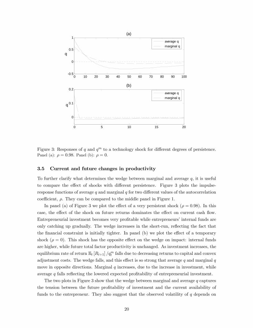
Figure 3: Responses of q and qm to a technology shock for different degrees of persistence.Panel (a): ρ = 0.98. Panel (b): ρ = 0.
3.5 Current and future changes in productivity
To further clarify what determines the wedge between marginal and average q, it is useful
to compare the effect of shocks with different persistence. Figure 3 plots the impulse-
response functions of average q and marginal q for two different values of the autocorrelation
coefficient, ρ. They can be compared to the middle panel in Figure 1.
In panel (a) of Figure 3 we plot the effect of a very persistent shock (ρ = 0.98). In this
case, the effect of the shock on future returns dominates the effect on current cash flow.
Entrepreneurial investment becomes very profitable while entrepreneurs’ internal funds are
only catching up gradually. The wedge increases in the short-run, reflecting the fact that
the financial constraint is initially tighter. In panel (b) we plot the effect of a temporary
shock (ρ = 0). This shock has the opposite effect on the wedge on impact: internal funds
are higher, while future total factor productivity is unchanged. As investment increases, the
equilibrium rate of return Et [Rt+1] /qmt falls due to decreasing returns to capital and convex
adjustment costs. The wedge falls, and this effect is so strong that average q and marginal q
move in opposite directions. Marginal q increases, due to the increase in investment, while
average q falls reflecting the lowered expected profitability of entrepreneurial investment.
The two plots in Figure 3 show that the wedge between marginal and average q captures
the tension between the future profitability of investment and the current availability of
funds to the entrepreneur. They also suggest that the observed volatility of q depends on
20

the types of shocks hitting the economy. In Table 4 we report the ratio of the volatility
of q to the volatility of the investment rate, σ (q) /σ (IK), for different values of ρ. For
comparison, the value of the ratio σ (q) /σ (IK) for Compustat firms is equal to 27.18
In the frictionless benchmark, the ratio between asset price volatility and investment
volatility is equal to ξ, which we are keeping constant at 8.5. For values of ρ lower than 0.89
the presence of the financial friction tends to dampen asset price volatility. However, for
higher values of ρ, asset price volatility is amplified. For example, when ρ = 0.98 the
volatility of q doubles compared to frictionless case, although it is still smaller than in the
data. Highly persistent shocks to productivity help to obtain more volatile asset prices,
by generating variations in the long run expected return on entrepreneurial capital. The
role of shocks to future productivity in magnifying asset price volatility has recently been
emphasized in Abel and Eberly (2005), in the context of a model with no financial frictions,
but with decreasing returns and market power. This exercise suggests that a model with
constant returns and financial frictions can lead to similar conclusions. The highly persistent
shock considered here is a combination of a change in current productivity and a change
in future productivity. The explicit treatment of pure “news shocks,” only affecting future
productivity, is left to future work (Walentin (2007)).
ρ 0 0.25 .50 0.75 0.98 0.967
ξ 8.5 8.5 8.5 8.5 8.5 18
σ (q) /σ (IK) 1.9 2.3 3.4 5.5 16.5 27
σ (IK) /σ (CFK) 0.19 0.24 0.33 0.48 0.73 0.48
Table 4. Shock persistence and the volatility of q.
In Table 4 we also report the effects of different values of ρ on the volatility of in-
vestment σ (IK) /σ (CFK). High values of ρ tend to increase the volatility of investment
relative to the volatility of cash flow. When we increase ρ we can re-calibrate ξ to keep
σ (IK) /σ (CFK) = 0.48 (as in the baseline calibration above) and this leads to a further
increase in the volatility of q. In particular, setting ρ = 0.967 and ξ = 18, allows us to match
the empirical values of both σ (IK) /σ (CFK) and σ (q) /σ (IK) (see the last column of Ta-
ble 4). Although the model does well on these dimensions, the required adjustment costs
seems very high and this parametrization delivers an excessive degree of serial correlation
for cash flow. A relatively easy fix would be to introduce a combination of both temporary
shocks and shocks to long-run productivity. This would allow the model to deliver less serial
correlation, while at the same time having larger movements in q that are uncorrelated with
current investment. Again, this extension is better developed in a model that allows for a
richer set of shocks and is left to future work.18See footnote 14 for calculation method.
21

4 Firm-level Heterogeneity
So far, we have focused on an economy where all firms have the same productivity, and only
aggregate productivity shocks are present. This, together with the assumption of constant
returns to scale, implies that the investment rate, q, and cash flow (normalized by assets) are
identical across firms. The advantage of this approach is that it makes it easy to compare
our results to the classic Hayashi (1982) model. At the same time, this approach has its
limitations, given that the evidence on the relation between q and investment is largely
based on panel data. Therefore, it is useful to consider variations of the model that allow
for cross-sectional heterogeneity.
An immediate extension is to allow for multiple sectors. If we assume that labor and
capital are immobile across sectors, which may be a reasonable approximation in the short
run, then w and qo are sector-specific prices and each sector’s dynamics are analogous
to the aggregate dynamics studied above. Therefore, under this interpretation, all the
results presented so far apply to the multiple sector case. In this section, we pursue an
alternative extension, by introducing productivity differences across firms. Let Aj,t denote
the productivity of firm j. Newborn entrepreneurs receive an initial random draw Aj,t
from a given distribution Φ. From then on, individual productivity follows the stationary
process Aj,t = Γ (Aj,t−1, j,t) with j,t drawn from the discrete p.d.f. π ( j,t). To keep matters
simple, we abstract from aggregate uncertainty and assume that the realized cross-sectional
distribution of the shocks is always identical to the ex-ante distribution for each individual
firm. The details of this extension are presented in Appendix B.
Given the absence of aggregate uncertainty, aggregate capital is constant in this economy
and so is the wage w and the price of used capital qo. This also implies that qm is constant
and equal to 1. However, as long as the financial constraint is binding, average q is greater
than 1 and is different across firms. The assumption of constant returns to scale still helps
to simplify the problem, as it implies that the investment rate, average q, and the cash-
flow-to-assets ratio are independent of the individual firm’s assets kj,t. However, these three
variables are now functions of the firm’s productivity Aj,t and are given by the following
three equations,
IKj,t =(1− θ)Rj,t − 1
1− θβCE [Rj,t+1|Aj,t]− 1,
qj,t = βE (1− θ)E£¡γ + (1− γ)φj,t+1
¢Rj,t+1|Aj,t
¤+ θβCE [Rj,t+1|Aj,t] ,
CFKj,t = Rj,t − qo,
where the return per unit of capital, Rj,t, and the marginal value of entrepreneurial wealth,
φj,t, are now firm-specific variables.19
The three expressions above for IKj,t, qj,t, and CFKj,t, emphasize once more the tension
19Both Rj,t and φj,t are functions only of Aj,t, so the distributions of Rj,t+1 and φj,t+1 conditional onAj,t can be obtained from the law of motion Aj,t+1 = Γ (Aj,t, j,t+1).
22

between current and future changes in productivity discussed in subsection 3.5. On the one
hand, current returns, captured by Rj,t, affect positively both the investment rate and cash
flow, but have no effect on q, which is a purely forward-looking variable. On the other hand,
future returns, captured by E [Rj,t+1|Aj,t], affect positively investment and q, but have no
effects on current cash flows.
To study the implications of the model for investment regressions, we construct simulated
time-series from the model described and run the investment regression (23). In Table 5
we report the regression coefficients obtained from the simulated series, using the same
parameters as in Section 3.
a1 a2
Model with financial friction 0.116 1.023
Table 5. Investment regression. Firm-specific shocks.
Once more, financial frictions introduce a strong correlation between cash flow and in-
vestment, so that cash flow has a positive coefficient in the regression. Notice that both
coefficients a1 and a2 are now larger than in the corresponding line of Table 2 and larger
than their empirical counterpart. This is not surprising, given that firms now face essentially
zero adjustment costs. In this model, adjustment costs are only due to aggregate changes
in the capital stock, and with no aggregate uncertainty such changes are absent.20 Another
implication of the absence of adjustment costs is that investment is too volatile. The ratio
σ (IK) /σ (CFK) is equal to 1.34 in the simulated series, more than twice as large as in the
data.21 In our model we have essentially assumed “external adjustment costs,” by allowing
firms to trade homogeneous capital on the used capital market. A fully developed model
with firm-specific shocks clearly calls for the introduction of “internal adjustment costs,”
both to reduce investment volatility at the firm level and to obtain more realistic coeffi-
cients in investment regressions. However, with internal adjustment costs we lose analytical
tractability, as optimal investment rules are, in general, non-linear.
5 Conclusions
In this paper, we have developed a tractable framework to study the effect of financial
frictions on the joint dynamics of investment and of the value of the firm. The model shows
that, in the presence of financial frictions, q reflects future quasi-rents that will go to the
insider. This introduces a wedge between average and marginal q. The size of this wedge
20The parameter ξ is accordingly irrelevant for this version of the model.21Notice also that the frictionless model is not a very useful benchmark in this case, as it gives very
extreme and unrealistic results. Absent financial frictions all the capital stock in the economy would go,each period, to the single firm with the highest expected return on capital, while q would be constant andequal to 1.
23
is determined by the tension between current and future profitability. A firm with high
future productivity and low internal funds today will display a higher q. The reason for
this is that the growth of its capital stock is constrained relative to expected productivity,
and this raises the future marginal product of capital.
The paper focuses on the implications of the model for the correlation between invest-
ment, q and cash flow. In particular, we show that a model with financial frictions can help
to replicate the observed low correlation between q and investment, and the fact that cash
flow appears with a positive coefficient in standard investment regressions. However, the
model has a number of additional testable predictions on the response of investment and
asset prices to different types of shocks (shocks with different persistence, shocks affecting
current/future productivity), as discussed in Section 3.5. As we noticed, recent models with
market power and decreasing returns at the firm level also display rich dynamics follow-
ing shocks with different temporal patterns. Empirical work documenting the conditional
behavior of investment and q following these shocks, would provide an important testing
ground for both classes of models.
Throughout the paper, we have maintained Hayashi’s (1982) assumption of constant
returns to scale both in the production function and in adjustment costs. This has two
advantages. First, it greatly simplifies aggregation. Second, it allows us to focus on the
“pure” effect of the financial friction on investment regressions. Models with decreasing
returns at the firm level can produce deviations from q theory for independent reasons, so
it is useful, at this stage, to separate those effects from the effects due to imperfections in
financial contracts. At the same time, this choice leaves aside a number of interesting issues,
which seem especially relevant when one introduces firm-level heterogeneity, as we did in
Section 4.
In the paper we have focused on the case of small stochastic deviations from the steady
state. It is possible to extend the model to allow for “large” shocks, opening the door to
potentially interesting phenomena. In particular, with large shocks it is possible to have a
model where firms hold precautionary reserves, i.e., choose to reduce investment today in
order to buy financial securities as insurance against future shocks. This is another area
where equilibrium behavior will be very sensitive to the time profile of the shocks hitting
the firm.
Finally, in the model we have assumed that consumers are risk-neutral. It turns out that
the characterization result in Proposition 4 can be extended to economies with risk-averse
consumers. Such an extension, which we leave to future work, would be useful to analyze
the model’s implications for the aggregate behavior of interest rates and risk-premia.
24

Appendix
A. Proofs
Proof of Lemma 1Consider the problem
minko
G (k0, ko) + qoko. (24)
Suppose ko = κ (qo) is optimal for a given qo and k0 = 1. Constant returns to scale imply that, givenany k0, ko = κ (qo) k0 is a solution to problem (24) and the optimum is equal to (G (κ (qo) , 1) + qo) k0.Therefore, we can set
qm (X) ≡ G (κ (qo (X)) , 1) + qo (X) ,
completing the proof of the first part of the lemma. In a similar way, consider the problem
maxl
AF (k, l)− wl + qok, (25)
and suppose l = η (w, qo, A) is optimal for a given triple w, qo, A and k = 1. Constant returns
to scale imply that, given any k, l = η (w, qo, A) k is a solution to (25) and the optimum is
(AF (1, η (w, qo, A))− wη (w, qo, A) + qo) k. Setting
R (X) ≡ AF (1, η (w (X) , qo (X) , A))− w (X) η (w (X) , qo (X) , A) + qo (X)
completes the proof.
Proof of Lemma 2Let B̃ be the space of bounded functions φ : X→ [1,∞). Define the map T : B̃ → B̃ as follows
Tφ (X) =βE (1− θ)E [(γ + (1− γ)φ (H (X, 0)))R (H (X, 0))]
qm (X)− θβCE [R (H (X, 0))].
Let us first check that Tφ ∈ B̃ if φ ∈ B̃, so the map is well defined. Notice that conditions (6)-(7)
and βE < βC imply that(1− θ)βEE [R (H (X, 0))]
qm (X)− θβCE [R (H (X, 0))]> 1.
This implies that for any φ ∈ B̃ we have
βE (1− θ)E [(γ + (1− γ)φ (H (X, 0)))R (H (X, 0))]qm (X)− θβCE [R (H (X, 0))]
≥ βE (1− θ)E [R (H (X, 0))]qm (X)− θβCE [R (H (X, 0))]
> 1, (26)
showing that Tφ (X) ≥ 1. Assumption (8) implies that
βE (1− θ)E [R (H (X, 0))]qm (X)− θβCE [R (H (X, 0))]
≤ 1
1− γ,
so if φ (X) ≤M for all X ∈ X, then Tφ (X) ≤M/ (1− γ) for all X ∈ X, completing the argument.Next, we show that T satisfies Blackwell’s sufficient conditions for a contraction. The monotonic-
ity of T is easily established. To check that it satisfies the discounting property notice that if
25
φ0 = φ+ a, then
Tφ0 (X)− Tφ (X) =βE (1− γ) (1− θ)E [R (H (X, 0))]qm (X)− θβCE [R (H (X, 0))]
a < βEa,
where the inequality follows from assumption (8). Since T is a contraction a unique fixed point
exists and (26) immediately shows that φ (X) > 1 for all X.
Proof of Proposition 3Let φ be defined as in Lemma 2. We proceed by guessing and verifying that the value function
is V (k, b,X) = φ (X) (R (X) k − b). In the text, we have shown that, under this conjecture, the
no-default condition can be rewritten in the form (3’). Therefore, we can rewrite problem (P ) as
maxcE ,k0,b0(.),b0L(.)
cE + βE (1− γ)X0π ( 0) [φ (H (X, 0)) (R (H (X, 0)) k0 − b0 ( 0))] +
+βEγX0π ( 0) [R (H (X, 0)) k0 − b0L (
0)]
s.t. cE + qm (X) k0 ≤ R (X) k − d, (λ)
b = d+ βC
Ã(1− γ)
X0π ( 0) b0 ( 0) + γ
X0π ( 0) b0L (
0)
!, (μ)
b0 ( 0) ≤ θR (H (X, 0)) k0 for all 0, (ν ( 0)π ( 0))
b0L (0) ≤ θR (H (X, 0)) k0 for all 0, (νL ( 0)π ( 0))
cE ≥ 0, (τ c)k0 ≥ 0, (τk)
where, in parenthesis, we report the Lagrange multiplier associated to each constraint. The multipli-
ers of the no-default constraints are normalized by the probabilities π ( 0). The first-order conditionsfor this problem are
1− λ+ τ c = 0,
βEE£¡γ + (1− γ)φ0
¢R0¤− λqm (X) + θE [(ν + νL)R
0] + τk = 0,
−βE (1− γ)φ0π ( 0) + λβC (1− γ)π ( 0)− ν ( 0)π ( 0) = 0,
−βEγπ ( 0) + λβCγπ (0)− νL (
0)π ( 0) = 0,
where R0 and φ0 are shorthand for R (H (X, 0)) and φ (H (X, 0)). We want to show that the valuesfor cE , k0, b0 and b0L in the statement of the proposition are optimal. It is immediate to check
that they satisfy the problem’s constraints. To show that they are optimal we need to show that
τ c = λ − 1 > 0, τk = 0, and ν ( 0) , νL ( 0) > 0 for all 0. Setting τk = 0 the second first-order
condition gives us
λ =(1− θ)βEE
£¡γ + (1− γ)φ0
¢R0¤
qm (X)− θβCE [R0]
which, by construction, is equal to φ (X). Then we have
τ c = φ (X)− 1 > 0,
26
which follows from Lemma 2,
ν ( 0) = (1− γ) (βCφ (X)− βEφ (H (X, 0))) > 0,
which follows from condition (10), and
νL (0) = (1− γ) (βCφ (X)− βE) > 0,
which follows from φ (X) > 1 and βC > βE . Substituting the optimal values in the objective
function we obtain φ (X) (R (X) k − b) confirming our initial guess.
Proof of Proposition 4The proof is split in two steps. In the first step, we construct the steady-state equilibrium of the
deterministic economy with a binding financial constraint, in the second, we construct an equilibrium
of the stochastic economy. First, we derive a useful preliminary result. Applying the envelope
theorem to problems (24) and (25) (see the proof of Lemma 1), using the fact that, in equilibrium,
the ratio ko/k0 is equal to Kt/Kt+1, and the ratio l/k is equal to 1/Kt, and using condition (16),
we obtain the following expressions for qmt and Rt:
qmt =∂G (Kt+1,Kt)
∂Kt+1, (27)
Rt = At∂F (Kt, 1)
∂Kt− ∂G (Kt+1,Kt)
∂Kt. (28)
Step 1. (Deterministic steady state) Consider a deterministic model where At is constant and
equal to 1 in each period (recall that 1 is the unconditional mean of the stochastic process for At
in the stochastic model). We will derive the steady state of this deterministic model under the
assumption that the financial constraint is binding in equilibrium. Let the superscript SS denotes
steady-state values. In steady state the equilibrium conditions (16) and (27) give qo,SS = 1− δ and
qm,SS = 1. The law of motion for the capital stock (13) gives the steady-state condition¡1− θβCR
SS¢KSS = (1− γ) (1− θ)RSSKSS + γwSSlE , (29)
and (28) gives
RSS =∂F
¡KSS , 1
¢∂K
+ 1− δ. (30)
Substituting (30) in (29) we obtain
KSS =
µα (θβC + (1− γ) (1− θ)) + γ (1− α) lE1− (θβC + (1− γ) (1− θ)) (1− δ)
¶ 11−α
, (31)
and substituting back in (30) we get
RSS = α¡KSS
¢α−1+ 1− δ. (32)
By assumption, the model parameters are such that βRSS < 1. A necessary and sufficient
27

condition for this is that the model’s parameters satisfy
βE
µα
1− (θβC + (1− γ) (1− θ)) (1− δ)
α (θβC + (1− γ) (1− θ)) + γ (1− α) lE+ 1− δ
¶> 1. (33)
Then, the following two inequalities also hold
θβCRS < 1,
(1− γ) (1− θ)RSS
1− θβCRSS
< 1. (34)
To prove these inequalities, notice that there cannot be a steady state with a binding financial
constraint and KSS = 0. Otherwise, RSS would go to infinity, violating βERSS < 1. So KSS must
be strictly positive. Then, rearranging equation (29), it follows that
1− βCθRSS − (1− γ) (1− θ)RSS > 0,
which implies both inequalities in (34).
The inequality βRSS < 1 and the two inequalities in (34) correspond to conditions (6)-(8) in
Proposition 3. Condition (10) holds immediately, given that βE < βC . This confirms that the
entrepreneurs’ optimal behavior is consistent with (13) (and (29)).
For completeness, we can use the recursive definition (9) to derive the steady state value of φ (X)
φSS =(1− θ)βER
SS
1− θβCRSS
³γ + (1− γ)φSS
´.
Rearranging this equation confirms that φSS > 1.
Step 2. (Stability) Substituting (15), (28) and the lagged version of (14) into (13), we obtain the
following second-order stochastic difference equation for Kt
Kt+1 =(1− γ) (1− θ)
³At
∂F (Kt,1)∂Kt
− ∂G(Kt+1,Kt)∂Kt
´Kt + γAt
∂F (Kt,1)∂L lE
∂G(Kt+1,Kt)∂Kt
− θβCEth³At+1
∂F (Kt+1,1)∂Kt+1
− ∂G(Kt+2,Kt+1)∂Kt+1
´i .
Linearizing this equation (under the functional assumptions made in the text) we get the following
second order equation for kt = lnKt − lnKSS ,
α0kt + α1kt+1 + α2kt+2 = 0,
where
α0 = ξ + α (1− α) (γlE − (1− γ) (1− θ))¡KSS
¢α−1+ (RSS − ξ) (1− γ) (1− θ) ,
α1 = −ξ − 1 + βθRSS − βθ³ξ + α (1− α)
¡KSS
¢α−1´+ (1− γ) (1− θ) ξ,
α2 = βθξ.
Provided that
α21 − α0α2 > 0 (35)
it is possible to show that the steady state derived in Step 1 is saddle-path stable. Then, given
28
sufficiently small shocks we can construct a stochastic steady state whereKt varies in a neighborhood
of KSS . This gives us an ergodic distribution for the state vector X, with bounded support. We
can then establish the continuity of the function φ with respect to the parameters X and show that
φ (X) is bounded in [φ, φ]. Since (6)-(8) hold in the deterministic steady state, a continuity argument
shows that they hold in the stochastic steady state. Finally, A− A can be set so as to ensure that
the bounds for φ (X) satisfy
βCφ > βEφ.
This guarantees that condition (10) is also satisfied.
Notice that, by the arguments given, conditions (33) and (35) are sufficient to ensure that the
steady state satisfies conditions (i) and (ii) in the hypothesis of the proposition.
B. The model with firm-level heterogeneity
Let w and qo denote the constant values for the wage and the price of used capital. The (gross)
return per unit of capital is now defined as:
R (Aj,t) ≡ maxη
©Aj,tF (1, η)− wη + q0
ª,
where η is the labor to capital ratio. The state variables for an individual entrepreneur are now
kj,t, bj,t, and Aj,t. The entrepreneur’s problem is characterized by the Bellman equation:
V (k, b, A) = maxcE,k0,b0(.),b0L(.)
cE + βE (1− γ)E [V (k0, b0 ( 0) ,Γ (A, 0))] +
+βEγE [R (Γ (A, 0)) k0 − b0L (0)]
subject to
cE + k0 ≤ R (A) k − d,
b = d+ βC ((1− γ)E[b0 ( 0)] + γE[b0L ( 0)]) ,
b0 ( 0) ≤ θR (Γ (A, 0)) k0,
b0L (0) ≤ θR (Γ (A, 0)) k0.
The no-default constraints have been expressed as linear constraints, proceeding as we did in Propo-
sition 3.
Now the marginal value of entrepreneurial wealth, φ, is a function of the individual productivity
A and we have
φ (A) =βE (1− θ)E [(γ + (1− γ)φ (Γ (A, 0)))R (Γ (A, 0))]
1− θβCE [R (Γ (A, 0))].
The analogues to conditions (6)-(10) are now
βEE [R (Γ (A, 0))] > 1,
θβCE [R (Γ (A, 0))] < 1,
(1− γ) (1− θ)E [R (Γ (A, 0))]1− θβCE [R (Γ (A, 0))]
< 1,
29

and
φ (A) >βEβC
φ (Γ (A, 0)) .
Under these conditions the optimal individual policy can be derived as in Proposition 3, and we
obtain the following law of motion for the individual capital stock
k0 =(1− θ)R (A)
1− θβCE [R (Γ (A, 0))]k.
A newborn entrepreneur has initial wealth wlE . Putting together these conditions, the distribution
Φ and the law of motion Γ (A, 0), allows us to completely characterize the joint dynamics of k andA. Then, under appropriate assumptions, we obtain an ergodic joint distribution J (A, k) and check
that the wage rate w is consistent with the market clearing conditionZ[η (A) k] dJ (A, k) = 1,
where η (A) is the optimal labor to capital ratio for a firm with productivity A.
Proceeding as in subsection 2.5, we can define the financial value of a continuing firm j:
pj,t = φj,t (Rj,tkj,t − bj,t) + bj,t − dj,t.
Substitute for dj,t, using the budget constraint dj,t = Rj,tkj,t− kj,t+1, and the law of motion for the
capital stock
kj,t+1 =1
1− θβCE [Rj,t+1|Aj,t](Rj,tkj,t − bj,t) ,
to obtain
pj,t =
µφj,t +
θβCE [Rj,t+1|Aj,t]
1− θβCE [Rj,t+1|Aj,t]
¶(Rj,tkj,t − bj,t) .
Dividing both sides by kj,t+1 and using the recursive property of φj,t gives the following expression
for average q
qj,t = βE (1− θ)E£¡γ + (1− γ)φj,t+1
¢Rj,t+1|Aj,t
¤+ θβCE [Rj,t+1|Aj,t] .
For the investment rate notice that
IKj,t =1
kj,t
µ(1− θ)Rj,t
1− θβCE [Rj,t+1|Aj,t]kj,t − kj,t
¶,
which gives the expression in the text. For cash flow notice that Aj,tF (kj,t, l j,t)−wlj,t = Rj,tkj,t−qokj,t.
30
References
[1] Abel, A. and J. C. Eberly, 2004, “Q Theory Without Adjustment Costs and Cash Flow
Effects Without Financing Constraints,” mimeo, Wharton.
[2] Abel, A. and J. C. Eberly, 2005, “Investment, Valuation and Growth Options,” mimeo,
Wharton.
[3] Albuquerque, R. and H. A. Hopenhayn, 2004, “Optimal Lending Contracts and Firm
Dynamics,” Review of Economic Studies, Vol. 71(2), pp. 285-315.
[4] Atkeson, A. and Cole, H, 2005, “A Dynamic Theory of Optimal Capital Structure and
Executive Compensation,” NBER working paper 11083.
[5] Bernanke, B., M. Gertler, 1989, “Agency Costs, Net Worth, and Business Fluctua-
tions,” American Economic Review, Vol. 79(1), pp. 14-31.
[6] Bernanke, B., M. Gertler and S. Gilchrist, 2000, “The Financial Accelerator in a Quan-
titative Business Cycle Framework,” Handbook of Macroeconomics, North Holland.
[7] Biais, B., T. Mariotti, G. Plantin and J.-C. Rochet, 2007, “Dynamic Security Design:
Convergence to Continuous Time and Asset Pricing Implications,” Review of Economic
Studies, Vol. 74(2), pp. 345-390.
[8] Bond S. and J. Cummins, 2001, “Noisy Share Prices and the Q model of Investment,”
Institute for Fiscal Studies WP 01/22.
[9] Carlstrom, C. and T. S. Fuerst, 1997, “Agency Costs, Net Worth, and Business Fluc-
tuations: A Computable General Equilibrium Analysis,” American Economic Review,
Vol. 87, pp. 893-910.
[10] Chirinko, R., 1993, “Business Fixed Investment Spending: Modeling Strategies, Em-
pirical Results, and Policy Implications,” Journal of Economic Literature Vol. 31, pp.
1875-1911.
[11] Chirinko, R. and H. Schaller, 2001, “Business Fixed Investment and “Bubbles”: The
Japanese Case,” American Economic Review, Vol. 91(3), pp. 663-680.
[12] Christiano, L., R. Motto and M. Rostagno, 2003, “The Great Depression and the
Friedman-Schwartz Hypothesis,” Journal of Money, Credit and Banking, Vol. 35(6),
pp. 1119-1197.
[13] Clementi, G. and H. Hopenhayn, 2006, “A Theory of Financing Constraints and Firm
Dynamics,” Quarterly Journal of Economics, Vol. 121(1), pp. 229-265.
31

[14] Cooley, T., R. Marimon and V. Quadrini, 2004, “Aggregate Consequences of Limited
Contract Enforceability,” Journal of Political Economy, Vol. 112, pp. 817-847.
[15] Cooper, R. and J. Ejarque, 2001, “Exhuming q: Market Power vs. Capital Market
Imperfections,” NBER working paper 8182.
[16] Cooper, R. and J. Ejarque, 2003, “Financial Frictions and Investment: Requiem in q,”
Review of Economic Dynamics, Vol. 6, pp. 710-728.
[17] DeMarzo, P. and M. Fishman, 2007, “Agency and Optimal Investment Dynamics,”
Review of Financial Studies, Vol. 20(1), pp. 151-188.
[18] DeMarzo, P. and Y. Sannikov, 2006, “Optimal Security Design and Dynamic Capital
Structure in a Continuous-Time Agency Model,” Journal of Finance, Vol. 61(6), pp.
2681-2724.
[19] Erickson, T. and T. Whited, 2000, “Measurement Error and the Relationship Between
Investment and q,” Journal of Political Economy, Vol. 108, pp. 1027-1057.
[20] Faia, E. and T. Monacelli, 2007, “Optimal Interest Rate Rules, Asset Prices, and Credit
Frictions,” Journal of Economic Dynamics and Control, Vol. 31(10), pp. 3228-3254.
[21] Fazzari, S., G. Hubbard and B. Petersen, 1988, “Financing Constraints and Corporate
Investment,” Brooking Papers on Economic Activity, Vol. 1, pp. 141-195.
[22] Gertler, M., S. Gilchrist and F. Natalucci, 2007, “External Constraints on Monetary
Policy and the Financial Accelerator,” Journal of Money, Credit and Banking, Vol.
39(2-3), pp. 295-330.
[23] Gilchrist, S. and C. Himmelberg, 1995, “Evidence on the Role of Cash Flow for Invest-
ment,” Journal of Monetary Economics, Vol. 36, pp. 541-572.
[24] Gilchrist, S. and C. Himmelberg, 1998, “Investment, Fundamentals and Finance,”
NBER Macro Annual, B. Bernanke and J. Rotemberg eds., the MIT Press, Cambridge,
pp. 223-274.
[25] Gilchrist, S., C. Himmelberg and G. Huberman, 2005, “Do Stock Price Bubbles In-
fluence Corporate Investment?” Journal of Monetary Economics, Vol. 52(4), pages
805-827.
[26] Gomes, J., 2001, “Financing Investment,” American Economic Review, Vol. 91, pp.
1263-1285.
[27] Hayashi, F., 1982, “Tobin’s Marginal q, and Average q: A Neoclassical Interpretation,”
Econometrica, Vol. 50, pp. 215-224.
32

[28] Hennessy, C. and T. Whited, 2007, “How Costly Is External Financing? Evidence from
a Structural Estimation,” Journal of Finance, Vol. 62(4), pp. 1705-1745.
[29] Holmström, B. and J. Tirole, 1997, “Financial Intermediation, Loanable Funds, and
The Real Sector,” Quarterly Journal of Economics, Vol. 112, pp. 663-691.
[30] Hubbard, G., 1998, “Capital-Market Imperfections and Investment,” Journal of Eco-
nomic Literature, Vol. 36, pp. 193-225.
[31] Iacoviello, M., 2005, “House Prices, Borrowing Constraints, and Monetary Policy in
the Business Cycle,” American Economic Review, Vol. 95(3), pp. 739-764.
[32] Kaplan, S. and L. Zingales, 1997, “Do Investment-Cash Flow Sensitivities Provide
Useful Measures of Finance Constraints?” Quarterly Journal of Economics, Vol. 112,
pp. 169-215.
[33] Kiyotaki, N. and J. Moore, 1997, “Credit Cycles,” Journal of Political Economy, Vol.
105, pp. 211-248.
[34] Moyen, Nathalie, 2004, “Investment-Cash Flow Sensitivities: Constrained Versus Un-
constrained Firms,” Journal of Finance 59(5), pp. 2061-2092.
[35] Panageas, S., 2005, “The Neoclassical q Theory of Investment in Speculative Markets,”
mimeo, Wharton.
[36] Rauh, J. D., 2006, “Investment and Financing Constraints: Evidence from the Funding
of Corporate Pension Plans,” Journal of Finance, 61 (1), pp. 33-71.
[37] Sargent, T., 1980, “ ‘Tobin’s q’ and the Rate of Investment in General Equilibrium,”
Carnegie-Rochester Conference Series on Public Policy, Vol. 12, pp. 107-154.
[38] Schiantarelli, F. and G. Georgoutsos, 1990, “Monopolistic Competition and the Q
Theory of Investment,” European Economic Review, Vol. 34(5) , 1061-1078.
[39] Walentin, K., 2007, “Expectation Driven Business Cycles with Limited Enforcement,”
mimeo, Sveriges Riksbank.
33