General rights Copyright and moral rights for the publications made accessible in the public portal are retained by the authors and/or other copyright owners and it is a condition of accessing publications that users recognise and abide by the legal requirements associated with these rights.

• Users may download and print one copy of any publication from the public portal for the purpose of private study or research. • You may not further distribute the material or use it for any profit-making activity or commercial gain • You may freely distribute the URL identifying the publication in the public portal

If you believe that this document breaches copyright please contact us providing details, and we will remove access to the work immediately and investigate your claim.

Downloaded from orbit.dtu.dk on: Dec 21, 2017

Dynamic Modeling and Validation of a Biomass Hydrothermal Pretreatment Process - ADemonstration Scale Study

Prunescu, Remus Mihail; Blanke, Mogens; Jakobsen, Jon Geest; Sin, Gürkan

Published in:AIChE Journal

Link to article, DOI:10.1002/aic.14954

Publication date:2015

Document VersionPeer reviewed version

Link back to DTU Orbit

Citation (APA):Prunescu, R. M., Blanke, M., Jakobsen, J. G., & Sin, G. (2015). Dynamic Modeling and Validation of a BiomassHydrothermal Pretreatment Process - A Demonstration Scale Study. AIChE Journal, 61(12), 4235-4250. DOI:10.1002/aic.14954

Dynamic Modeling and Validation of a Biomass Hydrothermal

Pretreatment Process - A Demonstration Scale Study

Remus Mihail Prunescu1, Mogens Blanke1, Jon Geest Jakobsen2, and Gürkan Sin∗3

1Department of Electrical Engineering, Automation and Control Group, Technical

University of Denmark, Elektrovej Building 326, 2800, Kgs. Lyngby, Denmark2Department of Process Control and Optimization, DONG Energy Thermal Power A/S,

Nesa Allé 1, 2820, Gentofte, Denmark3CAPEC-PROCESS, Department of Chemical and Biochemical Engineering, Technical

University of Denmark, Søltofts Plads Buildings 227 and 229, 2800, Kgs. Lyngby, Denmark

Abstract

Hydrothermal pretreatment of lignocellulosic biomass is a cost effective technology for

second generation biorefineries. The process occurs in large horizontal and pressurized

thermal reactors where the biomatrix is opened under the action of steam pressure and

temperature to expose cellulose for the enzymatic hydrolysis process. Several by-products

are also formed, which disturb and act as inhibitors downstream. The objective of this

study is to formulate and validate a large scale hydrothermal pretreatment dynamic model

based on mass and energy balances, together with a complex conversion mechanism and

kinetics. The study includes a comprehensive sensitivity and uncertainty analysis, with

parameter estimation from real-data in the 178-185 ◦C range. To highlight the application

utility of the model, a state estimator for biomass composition is developed. The predic-

tions capture well the dynamic trends of the process, outlining the value of the model for

simulation, control design, and optimization for full-scale applications.

Note

This article has been accepted for publication and undergone full peer review but has not

been through the copyediting, typesetting, pagination and proofreading process which may lead

to differences between this version and the Version of Record. Please cite this article as doi:

10.1002/aic.14954.

∗Principal corresponding author. Tel.: +45 45252806; E-mail: gsi@kt.dtu.dk

1

doi: 10.1002/aic.14954

Introduction

Lignocellulosic biomass, e.g. wheat straw, corn stover, bagasse etc, consist of cellulose, hemicel-

lulose, lignin, ash, and a negligible amount of residues1. The cellulosic fibers contain glucose units,

which are necessary for biofuel production, but layers of hemicellulose and lignin make cellulose

hardly accessible. The goal of the pretreatment process is to relocate lignin, and partially hydrolyze

the hemicellulose, which opens the biomatrix for cellulose such that enzymes can easily access it in

the enzymatic hydrolysis process downstream2.

Chiaramonti et al.3 review various methods of pretreatment, e.g. autohydrolysis, steam ex-

plosion, acid hydrolysis, alkaline hydrolysis, and many others. Studies show that hydrothermal

pretreatment with steam excels in cost effectiveness and, therefore, has been commercialized in

large scale second generation biorefineries. Integrating the biorefinery with a power plant following

the Integration Biomass Utilization System (IBUS) also contributes to reducing costs4. The pretreat-

ment process partially depolymerizes hemicellulose creating several degradation and by-products,

i.e. organic acids, xylooligomers, xylose, and inhibitors, e.g. furfural and 5-HMF, which impact the

downstream processes. The organic acids, i.e. acetic, succinic and lactic acid influence the pH of

pretreated fibers and become an issue in the enzymatic hydrolysis process5. Xylooligomers and

xylose act as strong inhibitors of cellulose hydrolysis by enzymes6, while furfural and 5-HMF inhibit

the fermentation process7. Also carbohydrates react with degradation products such as furfural to

create spherical droplets with lignin like structure named pseudo-lignin, which can degrade the

enzymatic activity8. Experimental studies show that reactor temperature and retention time relate

to biomass conversion9.

Lavarack et al.10 formulate a mechanistic acid hydrolysis model capable of predicting cellulose,

xylan and furfural concentrations but no one evaluated the model for steam pretreatment, and

at a large scale. This model has been used in later studies for model-based optimization of

bioprocesses under uncertainty11 and biorefinery configurations12. Overend et al.13 present an

empirical modeling alternative known as the severity factor, which Petersen et al.9 validated in

laboratory experiments for xylan recovery and furfural formation. These models are incomplete

because: (1) they miss production of important by-products such as organic acids, xylooligomers,

and pseudo-lignin; and (2) assume a uniform thermal environment, which is not the case in a full

scale reactor14. This study extends the existing Lavarack et al.10 model to demonstration scale using

computational fluid dynamics techniques, taking into account temperature variations in a large

scale thermal reactor, and production of the above enumerated by-products. The model is then

calibrated and validated against real data that were logged throughout several hours of operation

at a demonstration scale facility.

This study also assesses the model reliability through a comprehensive sensitivity and uncertainty

analysis. The sensitivity analysis quantifies the importance of each model parameter and creates an

identifiable subset of parameters that is used for parameter estimation following the methodology

from Sin et al.15 and Prunescu and Sin5.

Samples of fibers were collected after the pretreatment process and were analyzed with near

infra-red instruments (NIR) to determine their composition. The model parameters are estimated

using the NIR readings. The uncertainty analysis determines a confidence interval for model

predictions and is carried with respect to both model and feed parameters following the method

from Sin et al.15. As a global sensitivity measure, the standardized regression coefficients (SRC) are

computed in order to identify the model parameters responsible for most of the variations in model

predictions16. A residual analysis follows to identify how much of the signal is represented by the

2

doi: 10.1002/aic.14954

model. The study ends with a model application as a state estimator by using a static Kalman filter.

The state estimator not only filters the NIR measurements but also predicts by-products formation

such as C5 sugars and inhibitors.

This study has the following structure: the Methods section gives an overview of a state of the

art demonstration scale biorefinery from where the real measurements were collected; a ModelDevelopment section follows, which formulates the mathematical model for the pretreatment process

along with the model analysis methodology; the Results and Discussion section presents the model

analysis and validation results, and the model application as a state estimator; the study ends with

a Conclusions section, which summarizes all findings.

Methods

Biorefinery Experimental Setup

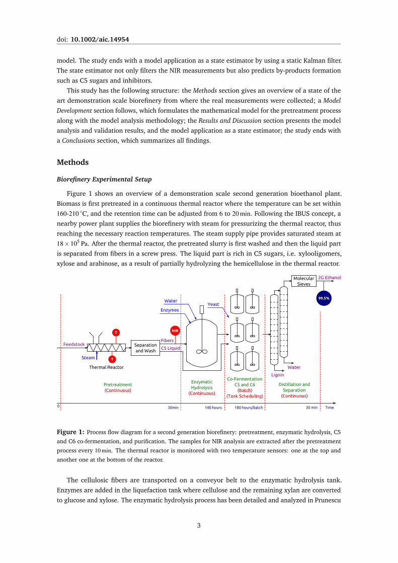
Figure 1 shows an overview of a demonstration scale second generation bioethanol plant.

Biomass is first pretreated in a continuous thermal reactor where the temperature can be set within

160-210 ◦C, and the retention time can be adjusted from 6 to 20 min. Following the IBUS concept, a

nearby power plant supplies the biorefinery with steam for pressurizing the thermal reactor, thus

reaching the necessary reaction temperatures. The steam supply pipe provides saturated steam at

18×105 Pa. After the thermal reactor, the pretreated slurry is first washed and then the liquid part

is separated from fibers in a screw press. The liquid part is rich in C5 sugars, i.e. xylooligomers,

xylose and arabinose, as a result of partially hydrolyzing the hemicellulose in the thermal reactor.

Figure 1: Process flow diagram for a second generation biorefinery: pretreatment, enzymatic hydrolysis, C5

and C6 co-fermentation, and purification. The samples for NIR analysis are extracted after the pretreatment

process every 10 min. The thermal reactor is monitored with two temperature sensors: one at the top and

another one at the bottom of the reactor.

The cellulosic fibers are transported on a conveyor belt to the enzymatic hydrolysis tank.

Enzymes are added in the liquefaction tank where cellulose and the remaining xylan are converted

to glucose and xylose. The enzymatic hydrolysis process has been detailed and analyzed in Prunescu

3

doi: 10.1002/aic.14954

and Sin5. The C5 and C6 sugars are then co-fermented for ethanol production in scheduled batch

reactors with genetically modified organisms (GMOs) for enhancing bioethanol production.

The purification and separation phase contains two distillation columns and molecular sieves.

Lignin is separated in the first distillation column, while ethanol is purified to 99.5 % in the second

column and in the molecular sieves. The recovered lignin is transported to an evaporation plant

and solidified as bio-pellets, which are sent to the nearby power plant for burning.

There is a timeline indicator at the bottom of Figure 1 showing the retention time for each

section of the biorefinery. The pretreatment process and distillation are the fastest processes with a

duration of maximum half an hour, while the enzymatic hydrolysis and fermentation can last 5 to 7

days each.

The demonstration scale facility has a processing capacity of 4000 kg/h of biomass17. Samples

of pretreated fibers were extracted after the pretreatment process every 10 min for a total duration

of 15 h. The samples were then analyzed with near infra-red instruments (NIR) to determine their

composition with respect to cellulose, xylan, lignin, acetic acid, and furfural. The thermal reactor

was monitored with two temperature sensors, one placed at the top of the tank for measuring the

temperature in the steam layer, and another one placed at the bottom of the reactor to measure the

biomass temperature.

Dataset

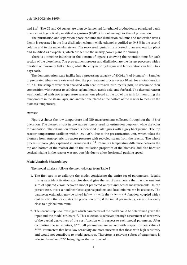
Figure 2 shows the raw temperature and NIR measurements collected throughout the 15 h of

operation. The dataset is split in two subsets: one is used for estimation purposes, while the other

for validation. The estimation dataset is identified in all figures with a grey background. The top

reactor temperature oscillates within 180-190 ◦C due to the pressurization unit, which takes the

biomass from atmospheric to reactor pressure with recycled steam from the reactor. The whole

process is thoroughly explained in Prunescu et al.14. There is a temperature difference between the

top and bottom of the reactor due to the insulation properties of the biomass, and also because

vertical mixing in the reactor was not possible due to a low horizontal pushing speed.

Model Analysis Methodology

The model analysis follows the methodology from Table 1:

1. The first step is to calibrate the model considering the entire set of parameters. Ideally,

this system identification exercise should give the set of parameters that has the smallest

sum of squared errors between model predicted output and actual measurements. In the

present case, this is a nonlinear least squares problem and local minima can be obstacles. The

parameter estimation may be solved in Matlab with the fminsearch function, coupled with a

cost function that calculates the prediction error, if the initial parameter guess is sufficiently

close to a global minimum.

2. The second step is to investigate which parameters of the model could be determined given the

input and the model structure18. This selection is achieved through assessment of sensitivity

of the partial derivatives of the cost function with respect to each model parameter. After

computing the sensitivities, δ msqr, all parameters are ranked with respect to their value of

δ msqr. Parameters that have low sensitivity are more uncertain that those with high sensitivity

and would not contribute to model accuracy. Therefore, a relevant subset of parameters is

selected based on δ msqr being higher than a threshold.

4

doi: 10.1002/aic.14954

175

180

185

190

T[◦

C]

Reactor Temperature

TopBottomEstimation setValidation set

10

20

30

40

C[%

]

NIR SolidsCelluloseXylanLigninEstimation setValidation set

0 2 4 6 8 10 12 14 16

4

6

Time [h]

C[g/k

g]

NIR SolublesAcidFurfuralEstimation setValidation set

Figure 2: The raw dataset. The top plot shows the reactor temperatures measured by the top and bottom

sensors. NIR offers information on the solid and soluble content of pretreated fibers. The whole dataset is split

into estimation and validation subsets.

3. In the third step the reduced set of parameters is identified using the NIR measurements

from the demonstration scale plant. The correlation matrix and standard deviations of the

estimates are also computed.

4. This step quantifies the prediction uncertainty. Having the covariance matrix and standard

deviations from the previous step allows Latin Hypercube Sampling (LHS)19 with correlation

control. The feed parameters is another source of uncertainty and is included in this analysis.

N Monte Carlo simulations are then run with sampled values and the 5th-95th percentiles

of the model predictions are found. A global sensitivity analysis follows by fitting a linear

model from parameters to model predictions and the standardized regression coefficients

are computed to identify which parameters are the most important for explaining the output

uncertainty.

5. The model estimation error or the residuals are analyzed in this step. A simulation is run

with the estimated parameters using the entire set of data (not only the estimation set). The

residuals distribution and autocorrelation are calculated in order to assess the quality of model

5

doi: 10.1002/aic.14954

predictions. A good model captures most of the signal in measurements and is characterized

by residuals being Gaussian with uncorrelated increments.

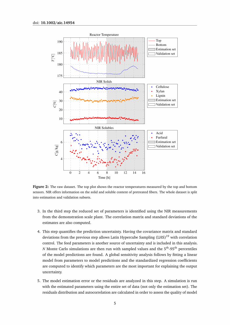
Table 1: Sensitivity and uncertainty analysis methodology. The output from step k−1 is the input to step k.

# Step Description Output

1 Model initialization • Initialization of all model parameters

to obtain a good working model fit;

θ0

2 Sensitivity analysis • List of significant parameters; δ msqr

• Find an identifiable parameter subset. θR0

3 Parameter estimation • Identify parameter subset; θR

• Correlation matrix; Rθ

• Confidence interval for parameters. σ

4 Uncertainty analysis • Calculate prediction uncertainty of the

model;

5th-95th percentile

• Sensitivity analysis with standardized

regression coefficients.

β

5 Residual analysis • Run simulation with the estimated pa-

rameters and using the entire dataset

• Check probability distribution of

model estimation errors or residuals

• Compute the autocorrelation function

Model Development

The mathematical model consists of mass and energy balances for the pretreatment process. In

large scale plants, the most common continuous thermal reactor is a long tank with cylindrical shape.

This study employs simplified computational fluid dynamics tools for modeling the composition

and temperature profiles.

Mass Balance

The thermal reactor has a continuous operation and the mass balance is established as the

accumulation of mass per unit of time equals the difference between inflow and outflow rates:

dMdt

= Fin−Fout (1)

where M is the total mass of biomass inside the reactor, Fin is the inflow rate of pressurized biomass

and Fout is the outflow rate of pretreated biomass.

Composition Balance

Pretreated fibers contain the following species: cellulose, xylan, arabinan, lignin, acetyl groups,

ash, glucose, xylooligomers, xylose, organic acids, furfural, 5-HMF, and other components in

negligible amounts. The change of species concentration with respect to time is a combination of

6

doi: 10.1002/aic.14954

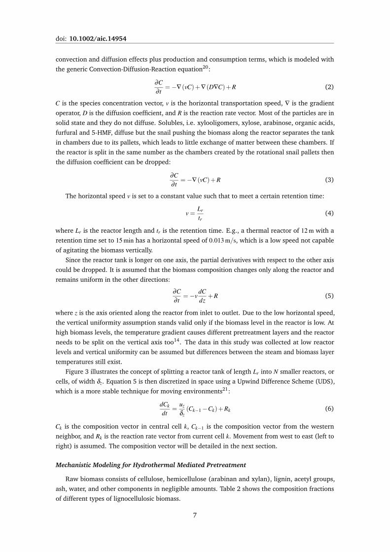
convection and diffusion effects plus production and consumption terms, which is modeled with

the generic Convection-Diffusion-Reaction equation20:

∂C∂ t

=−∇(vC)+∇(D∇C)+R (2)

C is the species concentration vector, v is the horizontal transportation speed, ∇ is the gradient

operator, D is the diffusion coefficient, and R is the reaction rate vector. Most of the particles are in

solid state and they do not diffuse. Solubles, i.e. xylooligomers, xylose, arabinose, organic acids,

furfural and 5-HMF, diffuse but the snail pushing the biomass along the reactor separates the tank

in chambers due to its pallets, which leads to little exchange of matter between these chambers. If

the reactor is split in the same number as the chambers created by the rotational snail pallets then

the diffusion coefficient can be dropped:

∂C∂ t

=−∇(vC)+R (3)

The horizontal speed v is set to a constant value such that to meet a certain retention time:

v =Lr

tr(4)

where Lr is the reactor length and tr is the retention time. E.g., a thermal reactor of 12 m with a

retention time set to 15 min has a horizontal speed of 0.013 m/s, which is a low speed not capable

of agitating the biomass vertically.

Since the reactor tank is longer on one axis, the partial derivatives with respect to the other axis

could be dropped. It is assumed that the biomass composition changes only along the reactor and

remains uniform in the other directions:

∂C∂ t

=−vdCdz

+R (5)

where z is the axis oriented along the reactor from inlet to outlet. Due to the low horizontal speed,

the vertical uniformity assumption stands valid only if the biomass level in the reactor is low. At

high biomass levels, the temperature gradient causes different pretreatment layers and the reactor

needs to be split on the vertical axis too14. The data in this study was collected at low reactor

levels and vertical uniformity can be assumed but differences between the steam and biomass layer

temperatures still exist.

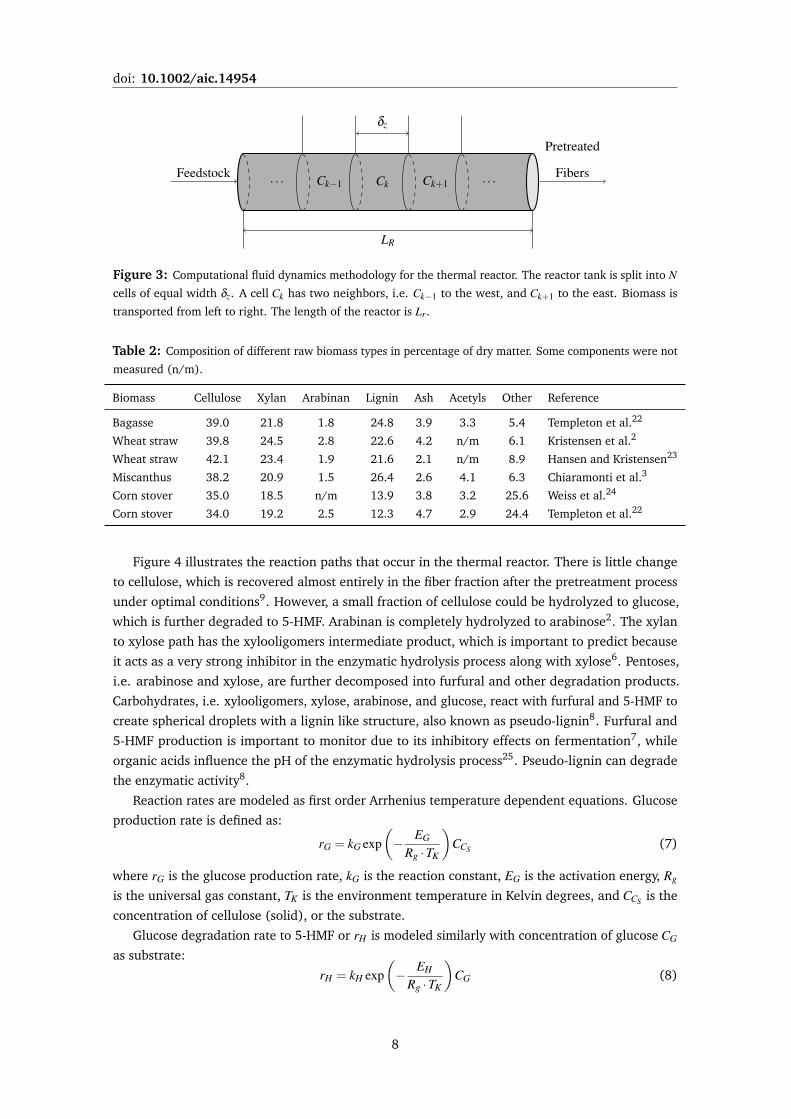
Figure 3 illustrates the concept of splitting a reactor tank of length Lr into N smaller reactors, or

cells, of width δz. Equation 5 is then discretized in space using a Upwind Difference Scheme (UDS),

which is a more stable technique for moving environments21:

dCk

dt=

uz

δz(Ck−1−Ck)+Rk (6)

Ck is the composition vector in central cell k, Ck−1 is the composition vector from the western

neighbor, and Rk is the reaction rate vector from current cell k. Movement from west to east (left to

right) is assumed. The composition vector will be detailed in the next section.

Mechanistic Modeling for Hydrothermal Mediated Pretreatment

Raw biomass consists of cellulose, hemicellulose (arabinan and xylan), lignin, acetyl groups,

ash, water, and other components in negligible amounts. Table 2 shows the composition fractions

of different types of lignocellulosic biomass.

7

doi: 10.1002/aic.14954

LR

Ck Ck+1Ck−1. . . . . .

δz

Feedstock

Pretreated

Fibers

Figure 3: Computational fluid dynamics methodology for the thermal reactor. The reactor tank is split into N

cells of equal width δz. A cell Ck has two neighbors, i.e. Ck−1 to the west, and Ck+1 to the east. Biomass is

transported from left to right. The length of the reactor is Lr.

Table 2: Composition of different raw biomass types in percentage of dry matter. Some components were not

measured (n/m).

Biomass Cellulose Xylan Arabinan Lignin Ash Acetyls Other Reference

Bagasse 39.0 21.8 1.8 24.8 3.9 3.3 5.4 Templeton et al.22

Wheat straw 39.8 24.5 2.8 22.6 4.2 n/m 6.1 Kristensen et al.2

Wheat straw 42.1 23.4 1.9 21.6 2.1 n/m 8.9 Hansen and Kristensen23

Miscanthus 38.2 20.9 1.5 26.4 2.6 4.1 6.3 Chiaramonti et al.3

Corn stover 35.0 18.5 n/m 13.9 3.8 3.2 25.6 Weiss et al.24

Corn stover 34.0 19.2 2.5 12.3 4.7 2.9 24.4 Templeton et al.22

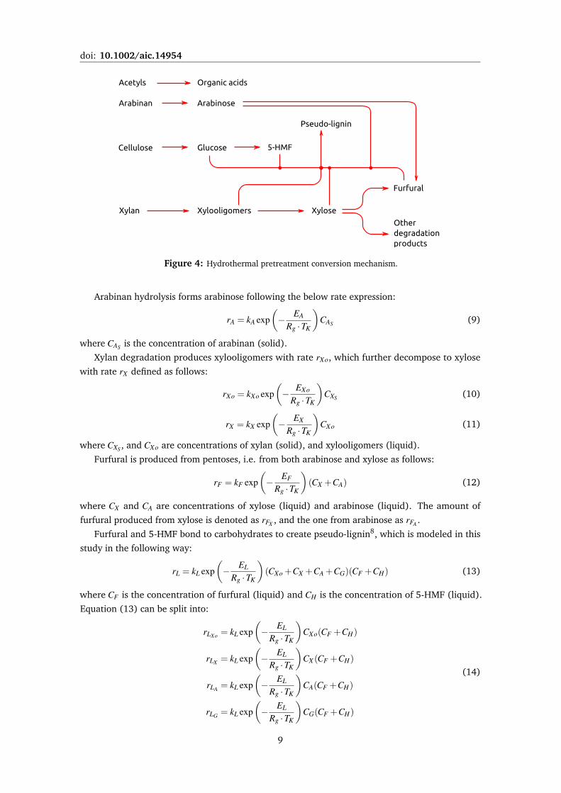
Figure 4 illustrates the reaction paths that occur in the thermal reactor. There is little change

to cellulose, which is recovered almost entirely in the fiber fraction after the pretreatment process

under optimal conditions9. However, a small fraction of cellulose could be hydrolyzed to glucose,

which is further degraded to 5-HMF. Arabinan is completely hydrolyzed to arabinose2. The xylan

to xylose path has the xylooligomers intermediate product, which is important to predict because

it acts as a very strong inhibitor in the enzymatic hydrolysis process along with xylose6. Pentoses,

i.e. arabinose and xylose, are further decomposed into furfural and other degradation products.

Carbohydrates, i.e. xylooligomers, xylose, arabinose, and glucose, react with furfural and 5-HMF to

create spherical droplets with a lignin like structure, also known as pseudo-lignin8. Furfural and

5-HMF production is important to monitor due to its inhibitory effects on fermentation7, while

organic acids influence the pH of the enzymatic hydrolysis process25. Pseudo-lignin can degrade

the enzymatic activity8.

Reaction rates are modeled as first order Arrhenius temperature dependent equations. Glucose

production rate is defined as:

rG = kG exp(− EG

Rg ·TK

)CCS (7)

where rG is the glucose production rate, kG is the reaction constant, EG is the activation energy, Rg

is the universal gas constant, TK is the environment temperature in Kelvin degrees, and CCS is the

concentration of cellulose (solid), or the substrate.

Glucose degradation rate to 5-HMF or rH is modeled similarly with concentration of glucose CG

as substrate:

rH = kH exp(− EH

Rg ·TK

)CG (8)

8

doi: 10.1002/aic.14954

Figure 4: Hydrothermal pretreatment conversion mechanism.

Arabinan hydrolysis forms arabinose following the below rate expression:

rA = kA exp(− EA

Rg ·TK

)CAS (9)

where CAS is the concentration of arabinan (solid).

Xylan degradation produces xylooligomers with rate rXo, which further decompose to xylose

with rate rX defined as follows:

rXo = kXo exp(− EXo

Rg ·TK

)CXS (10)

rX = kX exp(− EX

Rg ·TK

)CXo (11)

where CXS , and CXo are concentrations of xylan (solid), and xylooligomers (liquid).

Furfural is produced from pentoses, i.e. from both arabinose and xylose as follows:

rF = kF exp(− EF

Rg ·TK

)(CX +CA) (12)

where CX and CA are concentrations of xylose (liquid) and arabinose (liquid). The amount of

furfural produced from xylose is denoted as rFX , and the one from arabinose as rFA .

Furfural and 5-HMF bond to carbohydrates to create pseudo-lignin8, which is modeled in this

study in the following way:

rL = kL exp(− EL

Rg ·TK

)(CXo +CX +CA +CG)(CF +CH) (13)

where CF is the concentration of furfural (liquid) and CH is the concentration of 5-HMF (liquid).

Equation (13) can be split into:

rLXo = kL exp(− EL

Rg ·TK

)CXo(CF +CH)

rLX = kL exp(− EL

Rg ·TK

)CX (CF +CH)

rLA = kL exp(− EL

Rg ·TK

)CA(CF +CH)

rLG = kL exp(− EL

Rg ·TK

)CG(CF +CH)

(14)

9

doi: 10.1002/aic.14954

which denote pseudo-lignin produced from xylooligomers, xylose, arabinose and glucose when they

bind to both furfural and 5-HMF. Then Equation (13) becomes:

rL = rLXo + rLX + rLA + rLG (15)

Equation (13) can also be split into:

rLF = kL exp(− EL

Rg ·TK

)(CXo +CX +CA +CG)CF

rLH = kL exp(− EL

Rg ·TK

)(CXo +CX +CA +CG)CH

(16)

where rLF is the production rate of pseudo-lignin with furfural participation, while in rLH 5-HMF

participates.

Acetyls are released during hemicellulose hydrolysis and lead to organic acids formation with

rate rAc:

rAc = kAc exp(− EAc

Rg ·TK

)CAcS (17)

where CAcS is the concentration of acetyl groups in the hemicellulose (solid).

The composition vector Ck from Equation (6) contains all components from the mechanistic

scheme. The reaction rates from this section are put into a reaction rates vector Rk. Ck and Rk are

shown next in vector form:

Ck =

CCS

CXS

CAS

CLS

CAcS

CG

CXo

CX

CA

CAc

CF

CH

CW

CO

Rk =

−rG

−rXo

−rA

rL

−rAc

rG− rOG − (1−α)rLG

rXo− rX − (1−α)rLXo

rX − rFX − rOX − (1−α)rLX

rA− rOA − rFA − (1−α)rLA

rAc

rF −αrLF

rH −αrLH

0rOX + rOG + rOA

(18)

where CW is the water content, and α is a stoichiometric parameter for furfural and 5-HMF

participation in pseudo-lignin formation. In order to close the mass balance, the sum of all elements

in Rk has to be 0, and the sum of all elements in vector Ck is 1000 g/kg at any time t:

∑Rk = 0g/(kgs) ∑Ck = 1000g/kg (19)

Energy Balance

The steam layer energy balance together with a temperature controller for the thermal reactor

have been formulated in Prunescu et al.26. The energy balance for the biomass layer has been

studied in Prunescu et al.14 and is simplified in this paper by a distributed parameters model on

one axis, which is discretized along the reactor, or the z axis:

dhdt

=−v∂h∂ z

+Qk⇒dhk

dt=

vδ z

(hk−1−hk)+Qk (20)

10

doi: 10.1002/aic.14954

v is the horizontal speed, hk is the biomass enthalpy in cell k and hk−1 is the enthalpy in the western

neighbor. Qk represents the transfer of energy from steam to biomass in cell k. As part of this

coupled partial differential equation (PDE) system, the bottom and top temperature measurements

(sensors) are used to construct the boundary conditions. The PDE model is then solved for obtaining

the reactor temperature gradient, which is then utilized as the temperature of the reaction in

calculating the reaction rates vector Rk.

Steam is injected through the bottom of the reactor and gets in direct contact with the biomass.

The steam injection heat transfer is lumped into the boundary conditions of Equation (20). The

biomass is assumed to heat till the steam temperature near the inlet of the reactor, and used as a

western boundary condition. The heat transfer rate is computed as:

Q0 = Finh f −h0

hs0 −h0(21)

where Q0 is the heat transfer rate from the boundary conditions, Fin is the flow rate of biomass, h f

is the final enthalpy of heated biomass, h0 is the initial biomass enthalpy, and hs0 is the fresh steam

enthalpy. h0 is obtained by measuring the temperature of the biomass entering the reactor T0:

h0 = cb(T0−Tr) (22)

where cb is the specific heat of biomass, and Tr = 0 is the reference temperature. Biomass is assumed

to have a constant specific heat of approximately cb = 3.8kJ/kg, a value slightly lower than water

(4.18 kJ/kg) since the pretreatment slurry is a mix of condensed water and biomass.

hs0 is derived from saturated steam tables following the IAPWS-IF97 standard27 and from a

temperature sensor Ts0 mounted in the steam supply pipe:

hs0 = f (Ts0) (23)

h f is computed using the temperature of the steam layer Ts measured by the top temperature

sensor, and assuming that the biomass heats till the steam temperature near the reactor inlet:

h f = cb(Ts−Tr) (24)

It is natural to use the same grid in Equation (20) as the one from the composition balance

section. The model tracks the biomass enthalpy throughout each cell of the grid. The conductive

heat from the steam to the biomass layer is neglected due to the fact that biomass acts as an

insulator. Therefore, only convective effects remain in the biomass layer and Qk = 0,0 < k ≤ N.

The temperature profile is obtained by dividing the enthalpy from each cell with the specific

heat for biomass constant cb:

Tk =hk

cb(25)

where Tk is the biomass temperature from cell k, and cb is the specific heat of pretreated biomass.

Model Summary

The thermal reactor model tracks nC = 14 species concentrations shown in vector Ck from

Equation (18): cellulose, xylan, arabinan, lignin, acetyls, glucose, xylooligomers, xylose, arabinose,

acetic acid, furfural, 5-HMF, water, and other components.

The total number of states nx is variable depending on the initial value of N, the amount of cells

in the reactor grid. nx can be calculated as follows:

nx = N · (nC +nh)+(ns +nm) (26)

11

doi: 10.1002/aic.14954

where nC is the number of species, nh = 1 meaning one state for each grid cell enthalpy, ns = 2 is the

number of states from the steam layer (mass and enthalpy), and nm = 1 is the total mass of biomass

in the reactor. In this study, N is set to 10 leading to 153 states in total.

The model has 2 bus inputs: one for feedstock, and another one for steam. The feedstock input

has 16 components: flow rate (1), feedstock concentrations (14), and enthalpy (1). The steam

input has 2 components: flow rate (1), and enthalpy (1). In total there are 18 inputs.

There are 2 bus outputs: pretreated fibers and the liquid rich in C5 sugars. Each bus has 16components: flow rate (1), species concentrations (14), and enthalpy (1).

Table 3 shows the fixed model parameters. The kinetics parameters are determined in the model

calibration section of this study.

Table 3: Fixed model parameters. Feedstock is soaked before entering the thermal reactor till approximately

40 % dry matter.

Parameter Description Value Unit

Lr Thermal reactor length 12 m

tr Pretreatment retention time 15 min

N Grid cell resolution 10 -

δ z Grid cell width 1.2 m

v Reactor horizontal speed 0.013 m/s

Fin Feedstock flow rate 6 kg/s

h0 Feedstock enthalpy 117 kJ/kg

hs0 Fresh steam enthalpy (saturated) 2795 kJ/kg

cb Specific heat of pretreated biomass (constant) 3.8 kJ/(kgK)

R Universal gas constant 8.3145 J/(molK)

C0 Feedstock composition:

Cellulose 160 g/kg

Xylan 95 g/kg

Arabinan 8 g/kg

Lignin 80 g/kg

Acetyls 16 g/kg

Glucose 0 g/kg

Xylooligomers 0 g/kg

Xylose 0 g/kg

Arabinose 0 g/kg

Acetic acid 0 g/kg

Furfural 0 g/kg

5-HMF 0 g/kg

Water 600 g/kg

Other 41 g/kg

1000 g/kg

Results and Discussion

This section is split into a model analysis and validation part, and the model application as a

state estimator. The model analysis and validation section contains the sensitivity and uncertainty

12

doi: 10.1002/aic.14954

analysis, parameter estimation, and residual analysis.

Model Analysis and Validation

Model Initialization

Model parameters are calibrated with respect to the following NIR measurements: cellulose,

xylan, lignin, acetic acid and furfural. The data were obtained from a demonstration scale thermal

reactor throughout 15 h of operation. Only a subset of 7 h is used for calibration and parameter

estimation, while the entire set of measurements is used for validation and residual analysis. The

measurements of cellulose, xylan and lignin are reported as percentage of dry matter, while acetic

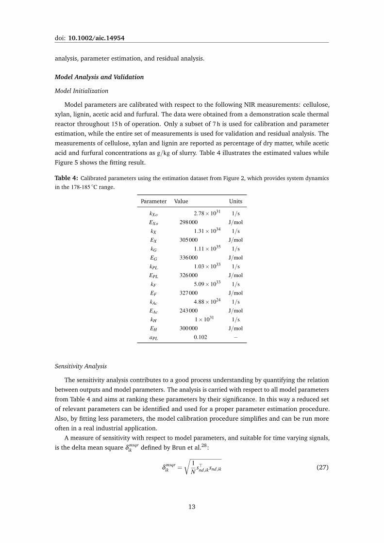
acid and furfural concentrations as g/kg of slurry. Table 4 illustrates the estimated values while

Figure 5 shows the fitting result.

Table 4: Calibrated parameters using the estimation dataset from Figure 2, which provides system dynamics

in the 178-185 ◦C range.

Parameter Value Units

kXo 2.78×1031 1/s

EXo 298000 J/mol

kX 1.31×1034 1/s

EX 305000 J/mol

kG 1.11×1035 1/s

EG 336000 J/mol

kPL 1.03×1033 1/s

EPL 326000 J/mol

kF 5.09×1033 1/s

EF 327000 J/mol

kAc 4.88×1024 1/s

EAc 243000 J/mol

kH 1×1031 1/s

EH 300000 J/mol

aPL 0.102 −

Sensitivity Analysis

The sensitivity analysis contributes to a good process understanding by quantifying the relation

between outputs and model parameters. The analysis is carried with respect to all model parameters

from Table 4 and aims at ranking these parameters by their significance. In this way a reduced set

of relevant parameters can be identified and used for a proper parameter estimation procedure.

Also, by fitting less parameters, the model calibration procedure simplifies and can be run more

often in a real industrial application.

A measure of sensitivity with respect to model parameters, and suitable for time varying signals,

is the delta mean square δ msqrik defined by Brun et al.28:

δ msqrik =

√1N

s>nd,iksnd,ik (27)

13

doi: 10.1002/aic.14954

10.0

20.0

30.0

40.0

C[%

]

CelluloseXylanLigninNIR CelluloseNIR XylanNIR Lignin

0 1 2 3 4 5 6 7

4.0

6.0

Time [h]

C[g/k

g]

AcidFurfuralNIR AcidNIR Furfural

Figure 5: Solid and liquid content of pretreated biomass: cellulose, xylan, lignin, acetic acid, and furfural.

where k is the parameter index, i is the model output index, N is the number of samples, and snd,ik

is a vector with the non dimensional sensitivity calculated in each sample:

snd,ik =∂yi

∂θk

θk

sci(28)

∂yi/∂θk represents the output variation with respect to parameter θk, and sci is a scaling factor with

the same physical dimension as the corresponding observation in order to make this measure non

dimensional. In this study, the scaling factor is chosen as the mean value of output i:

sci =1N

N

∑1

yi(k) (29)

All parameters are ranked according to δ msqrik for each output i. As the sensitivity measure

is non-dimensional, a cumulative variable is also defined as the sum of sensitivities for a given

parameter in all outputs. Because the model has to predict all defined outputs, the subset of

significant parameters contains all parameters with a cumulative sensitivity above a threshold,

which is set to 2 % of the maximum sensitivity. The cumulative delta mean square is defined as:

δ msqrk =

ny

∑i=1

δ msqrik (30)

where ny is the total number of outputs, i.e. ny = 5 in this study: concentrations of cellulose, xylan,

lignin, acetic acid, and furfural.

The same sensitivity analysis methodology has been applied on a cellulosic hydrolysis model in

previous studies by Sin et al.15, and Prunescu and Sin5.

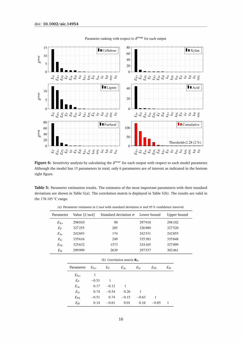
The sensitivity analysis results for the pretreatment process can be observed in Figure 6:

• Cellulose is mostly sensitive to EG, which is expected since cellulose is directly hydrolyzed

into glucose and this reaction is sensitive to the reactor temperature.

14

doi: 10.1002/aic.14954

• Xylan is sensitive to the activation energy of xylooligomers production EXo, which is not

surprising since xylooligomers are direct products of xylan hydrolysis.

• Lignin as percentage of dry matter follows the changes from xylan and cellulose content,

which is the solid content of biomass. This means that if more xylan is hydrolyzed then the

percentage of lignin in the remaining slurry after separation will increase. There is also lignin

production as pseudo-lignin and EPL is ranked second. EF , EG and EX influence the amount

of carbohydrates that participate in pseudo-lignin formation.

• Organic acids, mostly represented by acetic acid, is sensitive to the activation energy for

reaction rate rAc, i.e. EAc.

• The last output, furfural, is mostly sensitive to the activation energy EF of reaction rate rF . EXo

appears second because it directly affects the amount of xylose, which degrades to furfural.

The cumulative sensitivity measure is illustrated in the right bottom plot of Figure 6. The most

sensitive parameters are picked to be the first six:

θR = [EXo EF EAc EG EPL EH ] (31)

which are all activation energies directly involved in the reaction temperature dependency. This is

natural as it has been observed in experimental studies that small changes in reactor temperature

impact significantly the composition of pretreated fibers, and is in agreement with process expert

knowledge9. This analysis also ranks the activation energies among themselves. EXo (related

to xylooligomers production) is ranked first as the most sensitive parameter, which tells that

hemicellulose hydrolysis is the main phenomenon taking place in the reactor. EF is ranked second

showing that furfural is the main by-product followed by acetic acid (EAc). EG is ranked 4th,

which means that cellulose hydrolysis also occurs in the reactor but at a much lower rate than

hemicellulose hydrolysis. The other two by-products, i.e. pseudo-lignin and 5-HMF, have a lower

significance.

Parameter Estimation

The reduced set of parameters θR is identified based on the real NIR measurements from the

demonstration scale facility. A nonlinear least square method is run to obtain the parameter

estimates θR along with their standard deviation σ and correlation matrix Rθ . Table 5 shows the

results. The estimated parameter values are deemed credible as the parameter estimation error

indicated by the standard deviation is rather low, i.e. less than 1 %. However some of the parameter

estimates are found to be significantly correlated, e.g. correlation between EG and EXo is 0.74,

which implies poor identifiability. The reason for this is the dataset used for parameter estimation.

The data are obtained from an industrial scale facility during normal operational conditions under

small temperature disturbances. Such data with limited dynamics cannot be expected to provide

rich information for complete identification of all the parameters29 and design of experiments for

identification should be pursued on lower scale facilities. Other measurements should also be

included in the parameter estimation analysis, such as xylooligomers, xylose and glucose content of

the liquid part, which are missing in this study.

15

doi: 10.1002/aic.14954

EG

EX

oE

PL

EF

EA

cE

H k G k Xo

k PL

EX

k Ac

k F k H a PL k X

0

5

10

15

δmsq

r

Cellulose

EX

oE

GE

PL

EF

k Xo

EA

cE

H k G k PL

k Ac

EX k F k H k X a PL

0

20

40

60

80Xylan

EG

EX

oE

PL

EF

EH

EA

ck G k X

ok P

LE

X k F k H k Ac

a PL k X

0

5

10

δmsq

r

Lignin

EA

cE

GE

Xo

k Ac

EP

LE

FE

Hk X

ok G k P

LE

X k F k X k H a PL

0

20

40 Acid

EF

EX

oE

PL

EG k F EX

EH

k Xo

EA

ck P

La P

L k G k H k X k Ac

0

20

40

60

80

δmsq

r

Furfural

EX

oE

FE

Ac

EG

EP

LE

Hk X

oE

X k F k Ac

k G k PL

a PL

k H k X

0

50

100

Threshold=2.28 (2 %)

Cumulative

Parameter ranking with respect to δ msqr for each output

Figure 6: Sensitivity analysis by calculating the δ msqr for each output with respect to each model parameter.

Although the model has 15 parameters in total, only 6 parameters are of interest as indicated in the bottom

right figure.

Table 5: Parameter estimation results. The estimates of the most important parameters with their standard

deviations are shown in Table 5(a). The correlation matrix is displayed in Table 5(b). The results are valid in

the 178-185 ◦C range.

(a) Parameter estimates in J/mol with standard deviation σ and 95 % confidence interval.

Parameter Value [J/mol] Standard deviation σ Lower bound Upper bound

EXo 298010 98 297918 298102

EF 327255 285 326989 327520

EAc 242693 174 242531 242855

EG 335616 249 335383 335848

EPL 325632 1573 324165 327099

EH 299999 2639 297537 302461

(b) Correlation matrix Rθ .

Parameter EXo EF EAc EG EPL EH

EXo 1

EF −0.51 1

EAc 0.17 −0.12 1

EG 0.74 −0.54 0.26 1

EPL −0.51 0.74 −0.15 −0.63 1

EH 0.14 −0.61 0.01 0.16 −0.85 1

16

doi: 10.1002/aic.14954

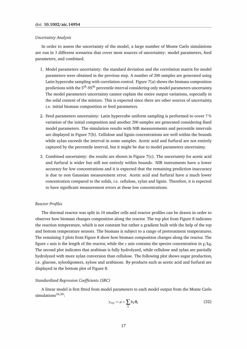
Uncertainty Analysis

In order to assess the uncertainty of the model, a large number of Monte Carlo simulations

are run in 3 different scenarios that cover most sources of uncertainty: model parameters, feed

parameters, and combined.

1. Model parameters uncertainty: the standard deviation and the correlation matrix for model

parameters were obtained in the previous step. A number of 200 samples are generated using

Latin hypercube sampling with correlation control. Figure 7(a) shows the biomass composition

predictions with the 5th-95th percentile interval considering only model parameters uncertainty.

The model parameters uncertainty cannot explain the entire output variations, especially in

the solid content of the mixture. This is expected since there are other sources of uncertainty,

i.e. initial biomass composition or feed parameters.

2. Feed parameters uncertainty: Latin hypercube uniform sampling is performed to cover 7 %variation of the initial composition and another 200 samples are generated considering fixed

model parameters. The simulation results with NIR measurements and percentile intervals

are displayed in Figure 7(b). Cellulose and lignin concentrations are well within the bounds

while xylan exceeds the interval in some samples. Acetic acid and furfural are not entirely

captured by the percentile interval, but it might be due to model parameters uncertainty.

3. Combined uncertainty: the results are shown in Figure 7(c). The uncertainty for acetic acid

and furfural is wider but still not entirely within bounds. NIR instruments have a lower

accuracy for low concentrations and it is expected that the remaining prediction inaccuracy

is due to non Gaussian measurement error. Acetic acid and furfural have a much lower

concentration compared to the solids, i.e. cellulose, xylan and lignin. Therefore, it is expected

to have significant measurement errors at these low concentrations.

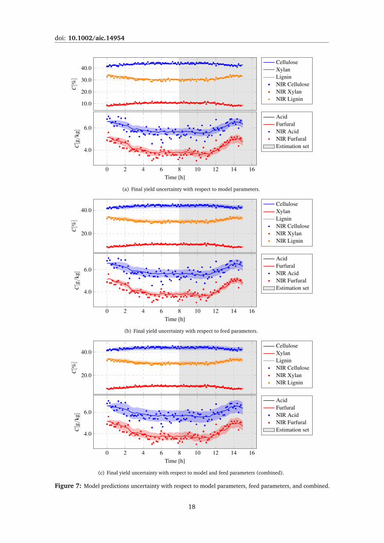
Reactor Profiles

The thermal reactor was split in 10 smaller cells and reactor profiles can be drawn in order to

observer how biomass changes composition along the reactor. The top plot from Figure 8 indicates

the reaction temperature, which is not constant but rather a gradient built with the help of the top

and bottom temperature sensors. The biomass is subject to a range of pretreatment temperatures.

The remaining 3 plots from Figure 8 show how biomass composition changes along the reactor. The

figure x axis is the length of the reactor, while the y axis contains the species concentration in g/kg.

The second plot indicates that arabinan is fully hydrolyzed, while cellulose and xylan are partially

hydrolyzed with more xylan conversion than cellulose. The following plot shows sugar production,

i.e. glucose, xylooligomers, xylose and arabinose. By-products such as acetic acid and furfural are

displayed in the bottom plot of Figure 8.

Standardized Regression Coefficients (SRC)

A linear model is first fitted from model parameters to each model output from the Monte Carlo

simulations16,30:

yreg = a+∑k

bkθk (32)

17

doi: 10.1002/aic.14954

10.0

20.0

30.0

40.0C[%

]

CelluloseXylanLigninNIR CelluloseNIR XylanNIR Lignin

0 2 4 6 8 10 12 14 16

4.0

6.0

Time [h]

C[g/k

g]

AcidFurfuralNIR AcidNIR FurfuralEstimation set

(a) Final yield uncertainty with respect to model parameters.

20.0

40.0

C[%

]

CelluloseXylanLigninNIR CelluloseNIR XylanNIR Lignin

0 2 4 6 8 10 12 14 16

4.0

6.0

Time [h]

C[g/k

g]

AcidFurfuralNIR AcidNIR FurfuralEstimation set

(b) Final yield uncertainty with respect to feed parameters.

20.0

40.0

C[%

]

CelluloseXylanLigninNIR CelluloseNIR XylanNIR Lignin

0 2 4 6 8 10 12 14 16

4.0

6.0

Time [h]

C[g/k

g]

AcidFurfuralNIR AcidNIR FurfuralEstimation set

(c) Final yield uncertainty with respect to model and feed parameters (combined).

Figure 7: Model predictions uncertainty with respect to model parameters, feed parameters, and combined.

18

doi: 10.1002/aic.14954

178

180

182

184

T[◦

C]

TemperatureUncertainty

0

50

100

C[g/k

g]

CelluloseUncertaintyXylanUncertaintyArabinanUncertaintyPseudo-ligninUncertainty

0

20

40

C[g/k

g]

GlucoseUncertaintyXylooligomersUncertaintyXyloseUncertaintyArabinoseUncertainty

0 2 4 6 8 10 120

2

4

6

Length [m]

C[g/

kg]

AcidUncertaintyFurfuralUncertainty

Figure 8: The top plot shows the reactor horizontal temperature gradient, which is used for calculating the

reaction rates. The other plots illustrate the reactor conversion profiles with confidence bounds due to both

model and feed parameters uncertainty.

19

doi: 10.1002/aic.14954

where yreg is the ith output, and a and bk are the linear model parameters. The standardized

regression coefficients β are a global sensitivity measure and are defined as:

βk =σθRk

σyi

bk (33)

where βk is the β coefficient, σθRkis the standard deviation of the parameter estimate, σyi is the

standard deviation of output i, and bk is the linear model parameter. βk is an indicator for how

much the parameter uncertainty contributes to the prediction uncertainty.

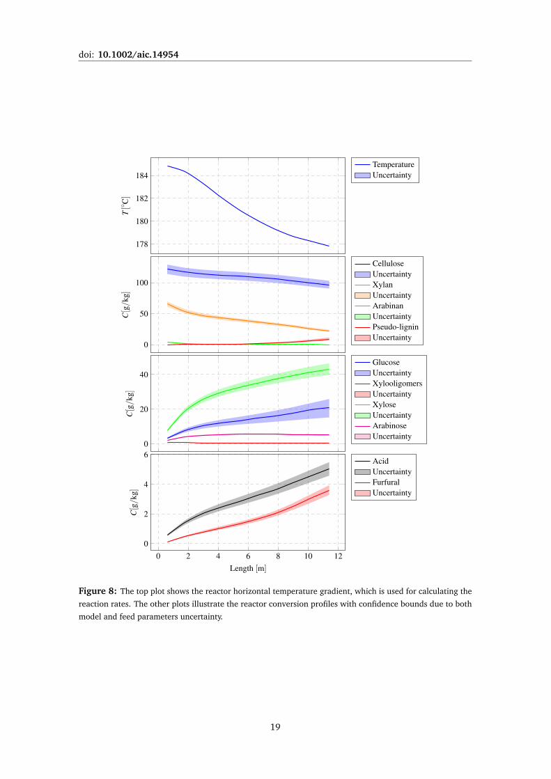
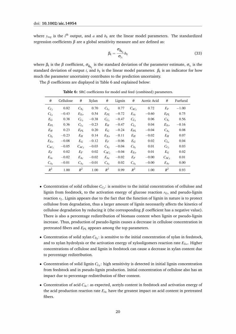
The β coefficients are displayed in Table 6 and explained below:

Table 6: SRC coefficients for model and feed (combined) parameters.

θ Cellulose θ Xylan θ Lignin θ Acetic Acid θ Furfural

CCS 0.82 CXS 0.70 CLS 0.77 CACS 0.72 EF −1.00

CLS −0.43 EXo 0.54 EPL −0.72 EAc −0.60 EPL 0.75

EG 0.38 CCS −0.38 CCS −0.47 CCS 0.06 CXS 0.56

EPL 0.36 CLS −0.23 EH −0.47 CLS 0.04 EXo −0.16

EH 0.23 EPL 0.20 EG −0.24 EPL −0.04 CAS 0.08

CXS −0.23 EH 0.14 EXo −0.11 EH −0.02 EH 0.07

EXo −0.08 EG −0.12 EF −0.06 EG 0.02 CLS 0.04

CACS −0.05 CACS −0.03 CXS −0.04 CXS 0.01 CCS 0.03

EF 0.02 EF 0.02 CACS −0.04 EXo 0.01 EG 0.02

EAc −0.02 EAc −0.02 EAc −0.02 EF −0.00 CACS 0.01

CAS −0.01 CAS −0.01 CAS 0.02 CAS −0.00 EAc 0.00

R2 1.00 R2 1.00 R2 0.99 R2 1.00 R2 0.93

• Concentration of solid cellulose CCS : is sensitive to the initial concentration of cellulose and

lignin from feedstock, to the activation energy of glucose reaction rG, and pseudo-lignin

reaction rL. Lignin appears due to the fact that the function of lignin in nature is to protect

cellulose from degradation, thus a larger amount of lignin necessarily affects the kinetics of

cellulose degradation by reducing it (the corresponding β coefficient has a negative value).

There is also a percentage redistribution of biomass content when lignin or pseudo-lignin

increase. Thus, production of pseudo-lignin causes a decrease in cellulose concentration in

pretreated fibers and EPL appears among the top parameters.

• Concentration of solid xylan CXS : is sensitive to the initial concentration of xylan in feedstock,

and to xylan hydrolysis or the activation energy of xylooligomers reaction rate EXo. Higher

concentrations of cellulose and lignin in feedstock can cause a decrease in xylan content due

to percentage redistribution.

• Concentration of solid lignin CLS : high sensitivity is detected in initial lignin concentration

from feedstock and in pseudo-lignin production. Initial concentration of cellulose also has an

impact due to percentage redistribution of fiber content.

• Concentration of acid CAc: as expected, acetyls content in feedstock and activation energy of

the acid production reaction rate EAc have the greatest impact on acid content in pretreated

fibers.

20

doi: 10.1002/aic.14954

• Concentration of furfural CF : activation energy of the furfural production reaction EF and

pseudo-lignin EPL are the most sensitive parameters. Furfural participates in pseudo-lignin

formation and is expected to find EPL among the top parameters.

Parameters related to feed composition have a higher sensitivity than the kinetic parameters,

even though only a deviation of 7 % was introduced in the initial biomass composition. This

indicates the importance of measuring the initial composition of feedstock for more accurate model

predictions. The SRC based sensitivity results are credible as the degree of linearization indicated

by Pearson correlation coefficient R2 is high for all the outputs16.

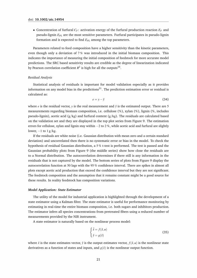
Residual Analysis

Statistical analysis of residuals is important for model validation especially as it provides

information on any model bias in the predictions31. The prediction estimation error or residual is

calculated as:

e = y− y (34)

where e is the residual vector, y is the real measurement and y is the estimated output. There are 5measurements regarding biomass composition, i.e. cellulose (%), xylan (%), lignin (%, includes

pseudo-lignin), acetic acid (g/kg) and furfural content (g/kg). The residuals are calculated based

on the validation set and they are displayed in the top plot series from Figure 9. The estimation

errors for cellulose, xylan and lignin stay within −2 to 2 %, while acetic acid and furfural are slightly

lower, −1 to 1 g/kg.

If the residuals are white noise (i.e. Gaussian distribution with mean zero and a certain standard

deviation) and uncorrelated then there is no systematic error or bias in the model. To check the

hypothesis of residual Gaussian distribution, a 5 % t-test is performed. The test is passed and the

Gaussian probability plots from Figure 9 (the middle series) show how close the residuals are

to a Normal distribution. The autocorrelation determines if there still is any information in the

residuals that is not captured by the model. The bottom series of plots from Figure 9 display the

autocorrelation function at 50 lags with the 95 % confidence interval. There are spikes in almost all

plots except acetic acid production that exceed the confidence interval but they are not significant.

The feedstock composition and the assumption that it remains constant might be a good source for

these results. In reality feedstock has composition variations.

Model Application: State Estimator

The utility of the model for industrial application is highlighted through the development of a

state estimator using a Kalman filter. The state estimator is useful for performance monitoring by

estimating in real-time the entire biomass composition, i.e. both sugars and inhibitors production.

The estimator infers all species concentrations from pretreated fibers using a reduced number of

measurements provided by the NIR instrument.

A state estimator is naturally based on the nonlinear process model:{ˆx = f (x,u)

y = g(x)(35)

where x is the state estimates vector, y is the output estimates vector, f (x,u) is the nonlinear state

derivatives as a function of states and inputs, and g(x) is the nonlinear output function.

21

doi: 10.1002/aic.14954

−2.0

0.0

2.0

Res

idua

ls[%

]Cellulose Xylan Lignin Acid

Res

idua

ls[g/k

g]

Furfural

0.05

0.5

0.95

Prob

abili

ty

0

0.5

1

Aut

ocor

rela

tion

Figure 9: Residual analysis for the validation set. The top plot series show the residuals; the middle series

compare in a Gaussian probability plot the distribution of residuals to a Normal distribution; the bottom series

display the autocorrelation function and the 95 % confidence interval.

Several methods exist for use of nonlinear process models in state estimation. Classical ap-

proaches include an extended Kalman filter for combined state and parameter estimation32 for a

linearized system at a particular point of operation, or direct inclusion of the nonlinear process

model in the filter33. Later developments have included the unscented Kalman and particle filters to

better explore and approximate non-Gaussian nature of the process noise in a nonlinear system34.

To compensate for model-mismatches between estimates and real measurements, an extra

correction term is added to the state derivatives equation from (35):{ˆx = f (x,u)+Le

y = g(x)(36)

where e is the estimation error defined in Equation (34), and L is a gain matrix that needs to be

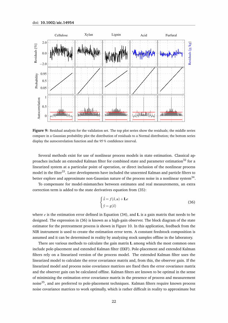
designed. The expression in (36) is known as a high-gain observer. The block diagram of the state

estimator for the pretreatment process is shown in Figure 10. In this application, feedback from the

NIR instrument is used to create the estimation error term. A constant feedstock composition is

assumed and it can be determined in reality by analyzing stock samples offline in the laboratory.

There are various methods to calculate the gain matrix L among which the most common ones

include pole-placement and extended Kalman filter (EKF). Pole-placement and extended Kalman

filters rely on a linearized version of the process model. The extended Kalman filter uses the

linearized model to calculate the error covariance matrix and, from this, the observer gain. If the

linearized model and process noise covariance matrices are fixed then the error covariance matrix

and the observer gain can be calculated offline. Kalman filters are known to be optimal in the sense

of minimizing the estimation error covariance matrix in the presence of process and measurement

noise35, and are preferred to pole-placement techniques. Kalman filters require known process

noise covariance matrices to work optimally, which is rather difficult in reality to approximate but

22

doi: 10.1002/aic.14954

Figure 10: State estimator block diagram. The state estimator uses 2 temperature sensors and the NIR

measurements to infer pretreated biomass composition. The state estimator acts both as measurement filter

and soft sensor.

alternatives exist, which estimate the noise structure online32, at the expense of more complexity of

the estimation algorithm.

The operational point in this study does not change significantly and this is the reason why a

static extended Kalman filter is chosen for the state estimator. The EKF design process follow these

steps:

1. The first step is to obtain a stochastic linear model by linearizing the nonlinear process model

from (35) around the nominal operational point seen in the datasets:{˙x = Ax+Bu+Gw

y = Cx+ v(37)

where A is the dynamic matrix of the linearized model, B is the input matrix, G is the state

noise propagation matrix, and C is the output matrix. State noise w and measurement noise v

are assumed to be 0 mean uncorrelated white noise sequences with variances Q and R:

w∼ (0,Q) v∼ (0,R) (38)

The linear model matrices are calculated by differentiating the nonlinear process model

around the nominal operational point (xe,ue):

A =∂ f (x,u)

∂ x

∣∣∣∣x=xe,u=ue

B =∂ f (x,u)

∂u

∣∣∣∣x=xe,u=ue

G =∂ f (x,u)

∂w

∣∣∣∣x=xe,u=ue

C =∂g(x)

∂ x

∣∣∣∣x=xe

(39)

23

doi: 10.1002/aic.14954

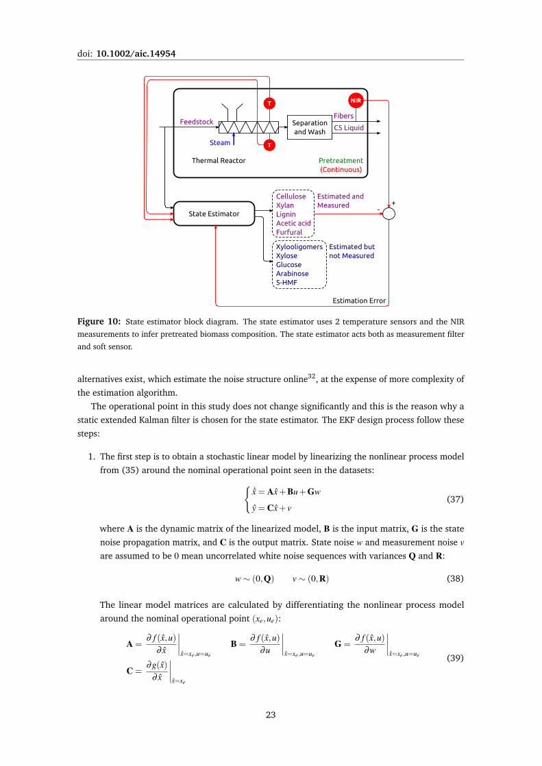
where xe and ue form the nominal operational point in terms of states and inputs. It is not

known how the process noise propagates inside the system dynamics, and G is set to Inx

(identity matrix of size nx or total number of states).

2. The second step is to approximate the state and measurement noise covariance matrices, i.e.

Q and R, which are set to:

Q = 10−4 · Inx R =

50 0 0 0 00 10 0 0 00 0 50 0 00 0 0 600 00 0 0 0 100

(40)

where Inx is an identity matrix, and nx is the number of states. The concentrations of solids

are higher and more reliable, therefore lower variances are used in the first 3 diagonal terms

from R, which correspond to cellulose, xylan and lignin (measured in % of dry matter). The

other 2 diagonal numbers are the variances for acetic acid and furfural (measured in g/kg),

which are in low concentrations and have larger measurement errors.

3. In the last step of the design process, the static Kalman gain is calculated35:

L = PCTR−1 (41)

where P is the error covariance matrix found from solving the Riccati equation35:

P = AP+PAT +GQGT−PCTR−1CP (42)

when P = 0.

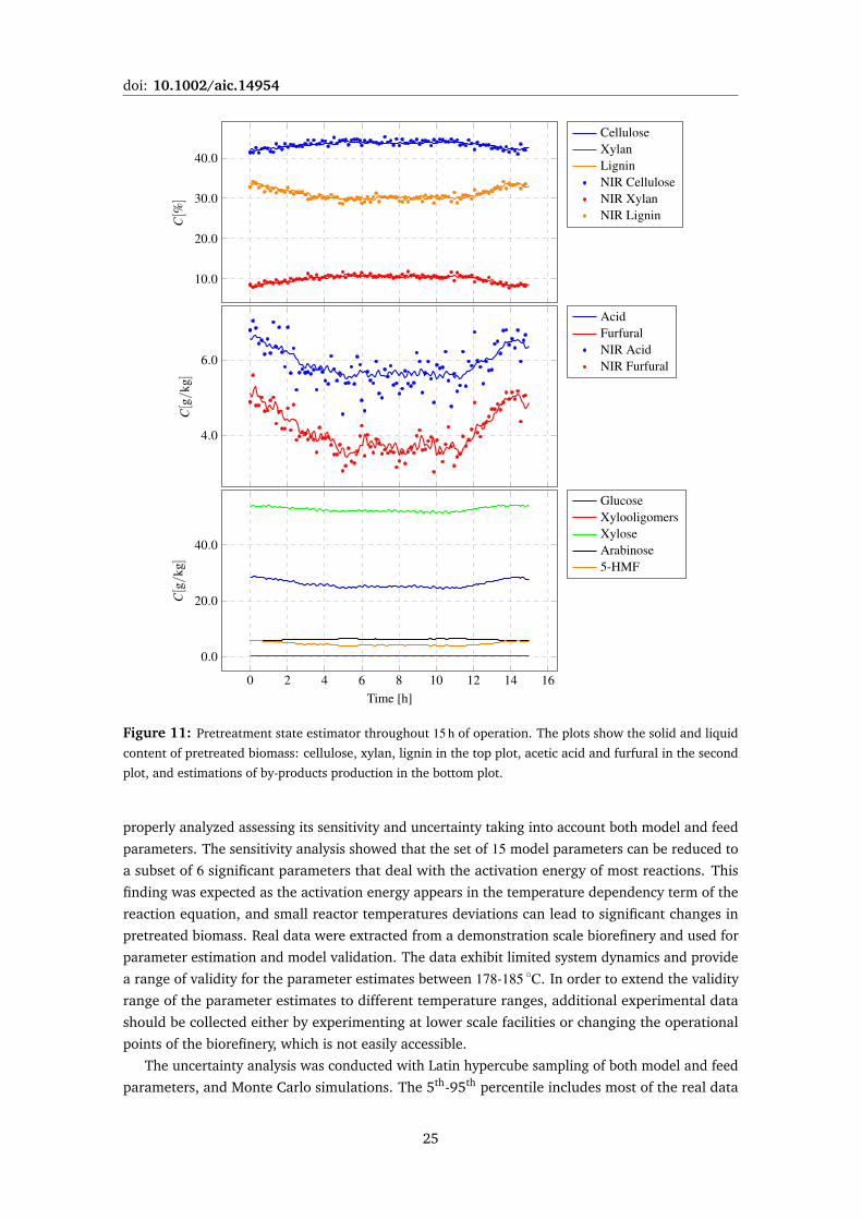
The Kalman state estimator is tested throughout the whole dataset of 15 h. Figure 11 shows the

model outputs overlapped with the NIR measurements. The model and the Kalman filter succeed in

following the dynamic trends of the process. The state estimator filters the NIR measurements and

also acts as a soft sensor for by-products production: glucose, xylooligomers, xylose, arabinose and

5-HMF shown in the bottom plot of Figure 11.

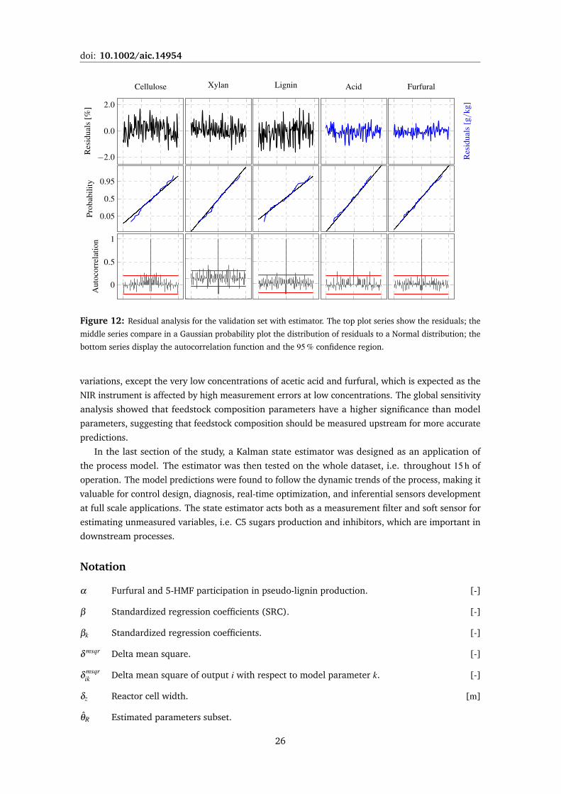
The residuals are displayed in Figure 12. The variance of the raw residuals is similar to the one

from Figure 9. However, the Kalman filter is able to capture more information from the process

causing the autocorrelation function to stay within the confidence interval (the bottom plot series

from Figure 12). The residuals distribution slightly change as indicated by the middle series of plots

from Figure 12. This happens because the noise covariance matrices, and the propagation of noise

through the system are unknown and set to arbitrary values.

The state estimator successfully embeds the real measurements to compensate on model

predictions mismatches under uncertainties such variation in feedstock composition or in model

parameters. Also, the state estimator acts as a soft sensor for several unmeasured variables,

some of which act as inhibitors in downstream processing especially in enzymatic hydrolysis and

fermentation. Such information includes: xylose, xylooligomers, arabinose, pseudo-lignin, glucose,

and 5-HMF production.

Conclusions

This study presented a dynamic model for a large scale biomass hydrothermal pretreatment

process. The model was capable of predicting the composition of pretreated fibers, and has been

24

doi: 10.1002/aic.14954

10.0

20.0

30.0

40.0C[%

]

CelluloseXylanLigninNIR CelluloseNIR XylanNIR Lignin

4.0

6.0

C[g/k

g]

AcidFurfuralNIR AcidNIR Furfural

0 2 4 6 8 10 12 14 16

0.0

20.0

40.0

Time [h]

C[g/

kg]

GlucoseXylooligomersXyloseArabinose5-HMF

Figure 11: Pretreatment state estimator throughout 15 h of operation. The plots show the solid and liquid

content of pretreated biomass: cellulose, xylan, lignin in the top plot, acetic acid and furfural in the second

plot, and estimations of by-products production in the bottom plot.

properly analyzed assessing its sensitivity and uncertainty taking into account both model and feed

parameters. The sensitivity analysis showed that the set of 15 model parameters can be reduced to

a subset of 6 significant parameters that deal with the activation energy of most reactions. This

finding was expected as the activation energy appears in the temperature dependency term of the

reaction equation, and small reactor temperatures deviations can lead to significant changes in

pretreated biomass. Real data were extracted from a demonstration scale biorefinery and used for

parameter estimation and model validation. The data exhibit limited system dynamics and provide

a range of validity for the parameter estimates between 178-185 ◦C. In order to extend the validity

range of the parameter estimates to different temperature ranges, additional experimental data

should be collected either by experimenting at lower scale facilities or changing the operational

points of the biorefinery, which is not easily accessible.

The uncertainty analysis was conducted with Latin hypercube sampling of both model and feed

parameters, and Monte Carlo simulations. The 5th-95th percentile includes most of the real data

25

doi: 10.1002/aic.14954

−2.0

0.0

2.0

Res

idua

ls[%

]Cellulose Xylan Lignin Acid

Res

idua

ls[g/k

g]

Furfural

0.05

0.5

0.95

Prob

abili

ty

0

0.5

1

Aut

ocor

rela

tion

Figure 12: Residual analysis for the validation set with estimator. The top plot series show the residuals; the

middle series compare in a Gaussian probability plot the distribution of residuals to a Normal distribution; the

bottom series display the autocorrelation function and the 95 % confidence region.

variations, except the very low concentrations of acetic acid and furfural, which is expected as the

NIR instrument is affected by high measurement errors at low concentrations. The global sensitivity

analysis showed that feedstock composition parameters have a higher significance than model

parameters, suggesting that feedstock composition should be measured upstream for more accurate

predictions.

In the last section of the study, a Kalman state estimator was designed as an application of

the process model. The estimator was then tested on the whole dataset, i.e. throughout 15 h of

operation. The model predictions were found to follow the dynamic trends of the process, making it

valuable for control design, diagnosis, real-time optimization, and inferential sensors development

at full scale applications. The state estimator acts both as a measurement filter and soft sensor for

estimating unmeasured variables, i.e. C5 sugars production and inhibitors, which are important in

downstream processes.

Notation

α Furfural and 5-HMF participation in pseudo-lignin production. [-]

β Standardized regression coefficients (SRC). [-]

βk Standardized regression coefficients. [-]

δ msqr Delta mean square. [-]

δ msqrik Delta mean square of output i with respect to model parameter k. [-]

δz Reactor cell width. [m]

θR Estimated parameters subset.

26

doi: 10.1002/aic.14954

x Estimated model states.

y Estimated model outputs. [%] or [g/kg]

L Kalman static gain.

Q State covariance matrix.

Rθ Model parameters correlation matrix.

R Output covariance matrix.

∇ Gradient operator. [-]

σ Model parameters standard deviation.

σθRkStandard deviation of parameter estimate k.

σyi Standard deviation of output i.

θ0 Initial model parameters.

θk Parameter k in vector θ .

θR0 Identifiable parameter subset.

a Linear model parameter used in SRC computations.

bk Linear model parameter used in SRC computations.

C Biomass composition vector. [g/kg]

Ck Composition vector in grid cell k. [g/kg]

CAS Concentration of arabinan (solid). [g/kg]

CAcS Concentration of acetyls (solid). [g/kg]

CA Concentration of arabinose (liquid). [g/kg]

cb Biomass specific heat constant. [kJ/(kgK)]

CCS Concentration of cellulose (solid). [g/kg]

CF Concentration of furfural (liquid). [g/kg]

CG Concentration of glucose (liquid). [g/kg]

CH Concentration of 5-HMF (liquid). [g/kg]

Ck−1 Composition vector in cell k−1. [g/kg]

CO Concentration of other components (liquid). [g/kg]

CW Concentration of water. [g/kg]

CXS Concentration of xylan (solid). [g/kg]

CXo Concentration of xylooligomers (liquid). [g/kg]

27

doi: 10.1002/aic.14954

CX Concentration of xylose (liquid). [g/kg]

D Diffusion coefficient. [m/s]

e Residual vector. [%] or [g/kg]

EG Glucose activation energy constant. [J/mol]

EAc Organic acid activation energy constant. [J/mol]

EA Arabinose activation energy constant. [J/mol]

EF Furfural activation energy constant. [J/mol]

EH 5-HMF activation energy constant. [J/mol]

EL Pseudo-lignin activation energy constant. [J/mol]

EXo Xylooligomers activation energy constant. [J/mol]

f (x,u) Nonlinear state derivatives function.

Fin Feedstock inflow rate. [kg/s]

Fout Pretreated biomass outflow rate. [kg/s]

g(x) Nonlinear model outputs function.

hk Biomass enthalpy in cell k. [kJ/kg]

h f Biomass final enthalpy after steam heating. [kJ/kg]

hk−1 Biomass enthalpy in cell k−1. [kJ/kg]

hs Fresh steam enthalpy (saturated steam). [kJ/kg]

kG Glucose reaction rate constant. [1/s]

kAc Organic acid reaction rate constant. [1/s]

kA Arabinose reaction rate constant. [1/s]

kF Furfural reaction rate constant. [1/s]

kH 5-HMF reaction rate constant. [1/s]

kL Pseudo-lignin reaction rate constant. [1/s]

kXo Xylooligomers reaction rate constant. [1/s]

Lr Thermal reactor length. [m]

M Mass of biomass in the thermal reactor. [kg]

N The thermal reactor is split into N cells. [-]

Q0 Lumped heat transfer from steam to biomass. [kJ/(kgs)]

Qk Energy transfer from steam to biomass in cell k. [kJ/(kgs)]

28

doi: 10.1002/aic.14954

Rg Universal gas constant. [J/(Kmol)]

rG Glucose production rate. [g/(kgs)]

Rk Reaction rate vector in cell k. [g/(kgs)]

rAc Organic acid production rate. [g/(kgs)]

rA Arabinose production rate. [g/(kgs)]

rFA Furfural production rate from arabinose. [g/(kgs)]

rFX Furfural production rate from xylose. [g/(kgs)]

rF Furfural production rate. [g/(kgs)]

rH 5-HMF production rate. [g/(kgs)]

rLA Pseudo-lignin production rate from arabinose. [g/(kgs)]

rLG Pseudo-lignin production rate from glucose. [g/(kgs)]

rLXo Pseudo-lignin production rate from xylooligomers. [g/(kgs)]

rLX Pseudo-lignin production rate from xylose. [g/(kgs)]

rL Pseudo-lignin production rate. [g/(kgs)]

rOA Arabinose degradation rate to other unidentified components. [g/(kgs)]

rOG Glucose degradation rate to other unidentified components. [g/(kgs)]

rOX Xylose degradation rate to other unidentified components. [g/(kgs)]

rXo Xylooligomers production rate. [g/(kgs)]

snd,ik Non dimensional sensitivity measure of output i with respect to parameter k. [-]

sci Scaling factor used in snd,ik.

T0 Feedstock temperature. [K]

TK Environment temperature in Kelvin degrees. [K]

Tk Biomass temperature in cell k. [K]

tr Retention time. [s]

Ts0 Steam supply temperature. [K]

v Horizontal transportation speed. [m/s]

y Model outputs: cellulose, xylan, lignin, acetic acid and furfural content. [%] or [g/kg]

yreg Linear model fit used in SRC computations.

29

doi: 10.1002/aic.14954

Literature Cited

1. Sluiter A, Hames B, Ruiz R, Scarlata C, Sluiter J, Templeton D, Crocker D. Determination of

structural carbohydrates and lignin in biomass. Technical Report NREL/TP-510-42618. 2008.

2. Kristensen JB, Thygesen LG, Felby C, Jørgensen H, Elder T. Cell-wall structural changes in

wheat straw pretreated for bioethanol production. Biotechnology for biofuels. 2008; 1:1–9.

3. Chiaramonti D, Prussi M, Ferrero S, Oriani L, Ottonello P, Torre P, Cherchi F. Review of pre-

treatment processes for lignocellulosic ethanol production, and development of an innovative

method. Biomass and Bioenergy. 2012; 46:25–35.

4. Larsen J, Petersen MØ, Thirup L, Li HW, Iversen FK. The IBUS Process – Lignocellulosic

Bioethanol Close to a Commercial Reality. Chemical Engineering & Technology. 2008; 31:765–

772.

5. Prunescu RM, Sin G. Dynamic modeling and validation of a lignocellulosic enzymatic hydroly-

sis process - A demonstration scale study. Bioresource Technology. 2013; 150:393–403.

6. Qing Q, Yang B, Wyman CE. Xylooligomers are strong inhibitors of cellulose hydrolysis by

enzymes. Bioresource technology. 2010; 101:9624–9630.

7. Cantarella M, Cantarella L, Gallifuoco A, Spera A, Alfani F. Effect of inhibitors released during

steam-explosion treatment of poplar wood on subsequent enzymatic hydrolysis and SSF.

Biotechnology progress. 2004; 20:200–206.

8. Sannigrahi P, Kim DH, Jung S, Ragauskas A. Pseudo-lignin and pretreatment chemistry. Energy

& Environmental Science. 2011; 4:1306–1310.

9. Petersen MØ, Larsen J, Thomsen MH. Optimization of hydrothermal pretreatment of wheat

straw for production of bioethanol at low water consumption without addition of chemicals.

Biomass and Bioenergy. 2009; 33:834–840.

10. Lavarack B, Griffin G, Rodman D. The acid hydrolysis of sugarcane bagasse hemicellulose

to produce xylose, arabinose, glucose and other products. Biomass and Bioenergy. 2002;

23:367–380.

11. Morales-Rodriguez R, Meyer AS, Gernaey KV, Sin G. A framework for model-based optimiza-

tion of bioprocesses under uncertainty: Lignocellulosic ethanol production case. Computers &

Chemical Engineering. 2012; 42:115–129.

12. Morales-Rodriguez R, Meyer AS, Gernaey KV, Sin G. Dynamic model-based evaluation of pro-

cess configurations for integrated operation of hydrolysis and co-fermentation for bioethanol

production from lignocellulose. Bioresource technology. 2011; 102:1174–1184.

13. Overend RP, Chornet E, Gascoigne JA. Fractionation of lignocellulosics by steam-aqueous pre-

treatments. Philosophical Transactions of the Royal Society of London. Series A, Mathematical

and Physical Sciences. 1987; 321:523–536.

14. Prunescu RM, Blanke M, Jensen JM, Sin G. Temperature Modelling of the Biomass Pretreat-

ment Process. Proceedings of the 17th Nordic Process Control Workshop. 2012:8–17.

15. Sin G, Meyer AS, Gernaey KV. Assessing reliability of cellulose hydrolysis models to sup-

port biofuel process design—Identifiability and uncertainty analysis. Computers & Chemical

Engineering. 2010; 34:1385–1392.

30

doi: 10.1002/aic.14954

16. Sin G, Gernaey KV, Neumann MB, Loosdrecht MCM van, Gujer W. Global sensitivity analysis

in wastewater treatment plant model applications: Prioritizing sources of uncertainty. Water

Research. 2011; 45:639–651.

17. Larsen J, Haven MØ, Thirup L. Inbicon makes lignocellulosic ethanol a commercial reality.

Biomass and Bioenergy. 2012; 46:36–45.

18. Walter E, Pronzato L. Identification of parametric models from experimental data. Springer,

1997.

19. Helton J, Davis F. Latin hypercube sampling and the propagation of uncertainty in analyses of

complex systems. Reliability Engineering & System Safety. 2003; 81:23–69.

20. Bird RB, Stewart WE, Lightfoot EN. Transport phenomena. John Wiley & Sons, 2007.

21. Egeland O, Gravdahl JT. Modeling and simulation for automatic control. Marine Cybernetics,

2002.

22. Templeton DW, Scarlata CJ, Sluiter JB, Wolfrum EJ. Compositional analysis of lignocellu-

losic feedstocks. 2. Method uncertainties. Journal of agricultural and food chemistry. 2010;

58:9054–9062.

23. Hansen MAT, Kristensen JB. Pretreatment and enzymatic hydrolysis of wheat straw (Triticum

aestivum L.)–The impact of lignin relocation and plant tissues on enzymatic accessibility.

Bioresource technology. 2011; 102:2804–2811.

24. Weiss ND, Farmer JD, Schell DJ. Impact of corn stover composition on hemicellulose conversion

during dilute acid pretreatment and enzymatic cellulose digestibility of the pretreated solids.

Bioresource technology. 2010; 101:674–678.

25. Prunescu RM, Blanke M, Sin G. Modelling and L1 adaptive control of pH in bioethanol

enzymatic process. Proceedings of the 2013 American Control Conference. 2013:1888–1895.

26. Prunescu RM, Blanke M, Sin G. Modelling and L1 Adaptive Control of Temperature in Biomass

Pretreatment. Annual Conference on Decision and Control. 2013:3152–3159.

27. Cooper JR, Dooley RB. Revised release on the IAPWS industrial formulation 1997 for the

thermodynamic properties of water and steam. The International Association for the Properties

of Water and Steam, 2007.

28. Brun R, Reichert P, Künsch HHR. Practical identifiability analysis of large environmental

simulation models. Water Resources Research. 2001; 37:1015–1030.

29. Holmberg A. On the practical identifiability of microbial growth models incorporating Michaelis-

Menten type nonlinearities. Mathematical Biosciences. 1982; 62:23–43.

30. Saltelli A, Ratto M, Andres T, Campolongo F, Cariboni J, Gatelli D, Saisana M, Tarantola S.

Global Sensitivity Analysis. The Primer. Chichester, UK: John Wiley & Sons, Ltd, 2007.

31. Power M. The predictive validation of ecological and environmental models. Ecological

Modelling. 1993; 68:33–50.

32. Ljung L. Asymptotic behavior of the extended Kalman filter as a parameter estimator for linear

systems. IEEE Transactions on Automatic Control. 1979; 24:36–50.

33. Zhou WW, Blanke M. Identification of a class of non-linear state space models using rpe

techniques. IEEE Transactions on Automatic Control. 1989; 34:312–316.

31

doi: 10.1002/aic.14954

34. Ristic B, Arulampalam S, Gordon N. Beyond the Kalman Filter: Particle Filters for Tracking

Applications. Artech House, 2004.

35. Brown RG, Hwang PYC. Introduction to Random Signals and Applied Kalman Filtering. 3rd ed.

John Wiley & Sons, 1996.

32