Fuel Etanol from Cellulosic Biomass

LEE R. LYND, JANET H. CusHmAN, ROBERTA J. NICHOLS, CHARLES E. WYMAN

Ethanol produced from cellulosic biomass is examined asa large-scale transportation fuel. Desirable features in-clude ethanol's fuel properties as well as benefits withrespect to urban air quality, global climate change, bal-ance of trade, and energy security. Energy balance, feed-stock supply, and environmental impact considerationsare not seen as significant barriers to the widespread useof fuel ethanol derived from cellulosic biomass. Conver-sion economics is the key obstacle to be overcome. In lightof past progress and future prospects for research-drivenimprovements, a cost-competitive process appears possi-ble in a decade.

A LTHOUGH FUEL ETHANOL IS CURRENTLY PRODUCED

from sugar cane in Brazil and from corn and other starch-rich grains in the United States, ethanol also can be made

from cellulosic materials such as wood, grass, and wastes. Thetechnology for ethanol production from cellulosic materials isfundamentally different from that for production from food crops.Failure to appreciate this difference has resulted in misconceptionsabout the potential of ethanol as a large-scale transportation fuel inthe United States. This artide reviews the current state and futurepotential of technology for producing ethanol from cellulosic bio-mass. The focus is on the use of ethanol as the primary fuelcomponent on a scale exceeding that possible with low-level etha-nol-gasoline blends.Of the four major energy sources in the United States, petroleum

supplies the largest share of total energy used and has the highestfraction imported, both by significant margins (Table 1). Thedomestic supply of conventional petroleum is also the most limitedofour major energy sources. Imported oil accounted for about 44%of the 1989 foreign trade deficit (1), and total petroleum expendi-tures were equal to about 2% of the gross national product (2, 3).This already prominent role for petroleum in the national economyis expected to increase as domestic oil exploration and productionbecome more expensive and as the cost and volume of importsincrease (4). Energy use by the transportation sector totaled 22 quad(1 quad = 1015 Btu) in 1989 and accounted for more than 60% oftotal petroleum consumption (2). Furthermore, the transportationsector, with its nearly total dependence on petroleum, has virtuallyno capacity to switch to other fuels in the event of a supplydisruption (5).

Air pollution is an important factor motivating interest in alter-

L. R. Lynd is with the Thayer School of Engineering, Dartmouth College, Hanover,NH 03755. J. H. Cushman manages the Biofuels Feedstock Development ProgramEnvironmental Sciences Division, Oak Ridge National Laboratory, Oak Ridge, TN37831. R. J. Nichols is with the Environmental and Safety Engineering Staff, FordMotor Company, Dearborn, MI 48121. C. E. Wyman manages the BiotechnologyResearch Branch, Solar Energy Research Institute, Golden, CO 80401.

1318

native fuels. At the local level, about 100 areas in the United Statesexceed national ambient air quality standards (NAAQS) for ozone(6), affecting more than half the population (7). Limits set by theNAAQS for carbon monoxide are exceeded in more than 40 areas(6). At the global level, carbon dioxide (CO2) is responsible formore than half the projected anthropically mediated climate change(8). Transportation fuels account for 27% of the 3.3 billion metrictons ofCO2 released annually in the United States from combustionof fossil fuels (9). Vehicles account for 4.7% of total worldwideanthropic CO2 emissions, with U.S. vehicles being responsible for2.5% of total emissions (10).

Ethanol as a FuelProduction and utilization. Fuel ethanol production by fermenta-

tion of starch crops is about 0.8 billion gallons (-0.06 quad) (11)in the United States, with ethanol selling for about $1.20 per gallon(12). The effective price to the blender is lowered by more than$0.50 per gallon by federal and state tax incentives (13, 14), withoutwhich fuel ethanol would not now be cost competitive.

Low-level ethanol-gasoline blends, consisting predominantly ofgasoline, may use ethanol directly or indirectly, the latter in the formofethyl tert-butyl ether (11, 15). About 7% ofall gasoline sold in theUnited States currently contains fermentation-derived ethanol, and10% blends are covered by the warranty of all U.S. automobilemanufacturers. Both direct and indirect blends increase octane andalso increase fuel oxygen content, facilitating more complete com-bustion in older cars.

Ethanol may be used as a primary fuel either in neat (unblended)form or with small amounts of gasoline. E1oo and E85 refer to neatethanol and an 85% ethanol-15% gasoline blend, respectively;similar terms are used for methanol. About 3 billion gallons ofethanol are used annually in Brazil, primarily as a neat fuel (14).Ethanol was used sporadically as a primary fuel in the first halfofthe20th century in both the United States and Europe (16). Fiat, Ford,General Motors, and Volkswagen have marketed automobiles de-signed for use ofhydrous (water-containing) ethanol in Brazil (17).

Alcohols are in many respects superior to gasoline as fuels forspark-ignited engines (18-20). Ethanol has fuel properties similar tothose ofmethanol; differences between the alcohols and gasoline aremuch greater than differences among the alcohols (20-22). Com-bustion of ethanol in internal combustion engines designed foralcohols will give higher thermal efficiency and power than combus-tion of gasoline in conventional engines (19, 20, 22). Ford hasconcluded that cold-starting problems have been solved for E85 andM85 for some applications, but not for Eioo or M1oo. A significantdevelopment for the use of alcohol fuels is the flexible fuel vehicle,which has the potential to operate on any mix ofethanol, methanol,and gasoline (5, 20).

Ford's experience, as well as estimates and data from others (23,

SCIENCE, VOL. 251

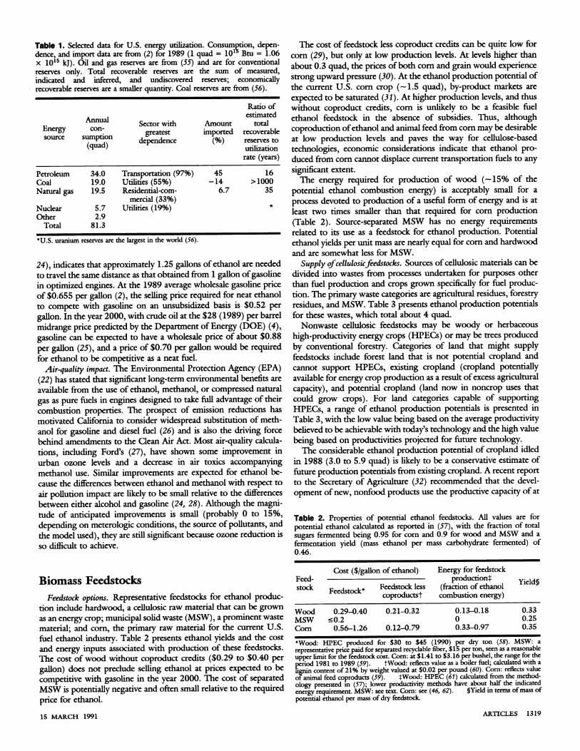
Table 1. Selected data for U.S. energy utilization. Consumption, depen-dence, and import data are from (2) for 1989 (1 quad = 10' Btu = 1.06x 1015 kI). Oil and gas reserves are from (55) and are for conventionalreserves only. Total recoverable reserves are the sum of measured,indicated and inferred, and undiscovered reserves; economicallyrecoverable reserves are a smaller quantity. Coal reserves are from (56).

Ratio ofestimatedAnnual Sector with Amount total

Energy con: greatest imported recoverablesource sumption dependence (%) reserves to

(quad) utilizationrate (years)

Petroleum 34.0 Transportation (97%) 45 16Coal 19.0 Utilities (55%) -14 >1000Natural gas 19.5 Residential-com- 6.7 35

mercial (33%)Nuclear 5.7 Utilities (19%) *Other 2.9

Total 81.3

*U.S. uranium reserves are the largest in the world (56).

24), indicates that approximately 1.25 gallons of ethanol are neededto travel the same distance as that obtained from 1 gallon ofgasolinein optimized engines. At the 1989 average wholesale gasoline priceof $0.655 per gallon (2), the selling price required for neat ethanolto compete with gasoline on an unsubsidized basis is $0.52 per

gallon. In the year 2000, with crude oil at the $28 (1989) per barrelmidrange price predicted by the Department of Energy (DOE) (4),gasoline can be expected to have a wholesale price of about $0.88per gallon (25), and a price of $0.70 per gallon would be requiredfor ethanol to be competitive as a neat fuel.

Air-quality impact. The Environmental Protection Agency (EPA)(22) has stated that significant long-term environmental benefits are

available from the use of ethanol, methanol, or compressed naturalgas as pure fuels in engines designed to take full advantage of theircombustion properties. The prospect of emission reductions hasmotivated California to consider widespread substitution of meth-anol for gasoline and diesel fuel (26) and is also the driving forcebehind amendments to the Clean Air Act. Most air-quality calcula-tions, including Ford's (27), have shown some improvement inurban ozone levels and a decrease in air toxics accompanyingmethanol use. Similar improvements are expected for ethanol be-cause the differences between ethanol and methanol with respect to

air pollution impact are likely to be small relative to the differencesbetween either alcohol and gasoline (24, 28). Although the magni-tude of anticipated improvements is small (probably 0 to 15%,depending on meterologic conditions, the source of pollutants, andthe model used), they are still significant because ozone reduction isso difficult to achieve.

Biomass FeedstocksFeedstock options. Representative feedstocks for ethanol produc-

tion include hardwood, a cellulosic raw material that can be grownas an energy crop; municipal solid waste (MSW), a prominent waste

material; and corn, the primary raw material for the current U.S.fuel ethanol industry. Table 2 presents ethanol yields and the cost

and energy inputs associated with production of these feedstocks.The cost of wood without coproduct credits ($0.29 to $0.40 per

gallon) does not preclude selling ethanol at prices expected to becompetitive with gasoline in the year 2000. The cost of separatedMSW is potentially negative and often small relative to the requiredprice for ethanol.

15 MARCH 1991

The cost of feedstock less coproduct credits can be quite low forcorn (29), but only at low production levels. At levels higher thanabout 0.3 quad, the prices of both corn and grain would experiencestrong upward pressure (30). At the ethanol production potential ofthe current U.S. corn crop (-1.5 quad), by-product markets areexpected to be saturated (31). At higher production levels, and thuswithout coproduct credits, corn is unlikely to be a feasible fuelethanol feedstock in the absence of subsidies. Thus, althoughcoproduction ofethanol and animal feed from corn may be desirableat low production levels and paves the way for cellulose-basedtechnologies, economic considerations indicate that ethanol pro-duced from corn cannot displace current transportation fuels to anysignificant extent.The energy required for production of wood (~15% of the

potential ethanol combustion energy) is acceptably small for aprocess devoted to production of a useful form of energy and is atleast two times smaller than that required for corn production(Table 2). Source-separated MSW has no energy requirementsrelated to its use as a feedstock for ethanol production. Potentialethanol yields per unit mass are nearly equal for corn and hardwoodand are somewhat less for MSW.

Supply ofcellulosiwfeedstocks. Sources of cellulosic materials can bedivided into wastes from processes undertaken for purposes otherthan fuel production and crops grown specifically for fuel produc-tion. The primary waste categories are agricultural residues, forestryresidues, and MSW. Table 3 presents ethanol production potentialsfor these wastes, which total about 4 quad.Nonwaste cellulosic feedstocks may be woody or herbaceous

high-productivity energy crops (HPECs) or may be trees producedby conventional forestry. Categories of land that might supplyfeedstocks include forest land that is not potential cropland andcannot support HPECs, existing cropland (cropland potentiallyavailable for energy crop production as a result of excess agriculturalcapacity), and potential cropland (land now in noncrop uses thatcould grow crops). For land categories capable of supportingHPECs, a range of ethanol production potentials is presented inTable 3, with the low value being based on the average productivitybelieved to be achievable with today's technology and the high valuebeing based on productivities projected for future technology.The considerable ethanol production potential of cropland idled

in 1988 (3.0 to 5.9 quad) is likely to be a conservative estimate offuture production potentials from existing cropland. A recent reportto the Secretary of Agriculture (32) recommended that the devel-opment of new, nonfood products use the productive capacity of at

Table 2. Properties of potential ethanol feedstocks. All values are forpotential ethanol calculated as reported in (57), with the fraction of totalsugars fermented being 0.95 for corn and 0.9 for wood and MSW and afermentation yield (mass ethanol per mass carbohydrate fermented) of0.46.

Cost ($/gallon of ethanol) Energy for feedstockFeed- productiontstock Feedstock* Feedstock less (fraction of ethanol YieldS

coproductst combustion energy)

Wood 0.29-0.40 0.21-0.32 0.13-0.18 0.33MSW 50.2 0 0.25Corn 0.56-1.26 0.12-0.79 0.33-0.97 0.35

*Wood: HPEC produced for $30 to $45 (1990) per dry ton (58). MSW: a

representative price paid for separated recyclable fiber, $15 per ton, seen as a reasonableupper limit for the feedstock cost. Corn: at $1.41 to $3.16 per bushel, the range for theperiod 1981 to 1989 (59). tWood: reflects value as a boiler fuel; calculated with a

lignin content of 21% by weight valued at $0.02 per pound (60). Corn: reflects valueof animal feed coproducts (59). *Wood: HPEC (61) calculated from the method-ology presented m (57); lower productivity methods have about half the indicatedenergy requirement. MSW: see text. Corn: see (46, 62). SYield in terms of mass ofpotential ethanol per mass of dry feedstock.

ARTICLES 1319

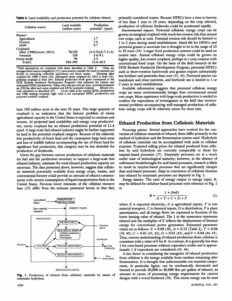
Table 3. Land availability and production potential for cellulose ethanol.

Land available ProductionCellulose source (million acres) potential* (quad)

WastestAgricultural 1.7Forestry 1.4MSW 0.7

CroplandtIdled (1988)/excess (2012) 78/150 (3-5.9)/(5.7-11.4)Potential 150 3.4-9.1

Forest lands 96 2.2Total 11 324-396 12.4-26.5

*Yield assumptions are consistent with those described in Table 2. tData areaverages from sources compiled in (57); most sources consider the need to maintain soilfertility in estimating collectible agricultural and forest wastes. tExisting idledcropland for 1988 is from (63); anticipated excess cropland for 2012 is from (32),potential cropland is from (64). Ethanol production levels given correspond to theDOE Biofuels Feedstock Development Program's best estimates for current andanticipated HPEC productivity. Values (dry tons per acre per year, current/anticipated)are 5/10 for idled and excess cropland and 3/8 for potential cropland. §From (31),with calculation as described (51). 11 Low value is for current HPEC productivityand 1988 existing cropland; high value is for anticipated HPEC productivity andprojected available cropland.

least 150 million acres in the next 25 years. This large quantity ofcropland is an indication that the historic problem of excessagricultural capacity in the United States is expected to continue andworsen. At projected land availability and energy crop productivi-ties, excess cropland has an ethanol production potential of 11.4quad. A large-scale fuel ethanol industry might be further supportedby land in the potential cropland category. Because of the relativelylow productivity of forest land and the consequent large land areasand loss of wildlife habitat accompanying the use of forest land forsignificant fuel production, this category may be less desirable forproduction of feedstocks.Given the gap between current production of cellulosic materials

for fuel and the production necessary to support a large-scale fuelethanol industry, estimates for total ethanol production capacity areuncertain. The data presented above, however, suggest that cellulo-sic materials potentially available from energy crops, wastes, andconventional forestry could provide an amount of ethanol commen-surate with current consumption ofliquid transportation fuels in theUnited States. Previous lower estimates of the cellulose resourcebase (33) differ from the estimate presented herein in that they

primarily considered wastes. Because HPECs have a time to harvestof less than 1 year to 10 years, depending on the crop selected,production of cellulosic feedstocks could be accelerated rapidly.

Environmental impacts. Perennial cellulosic energy crops can begrown on marginal cropland with much less erosion risk than annualrow crops, such as corn. Potential erosion risk should be limited to1 to 2 years during stand establishment. Stand life for HPECs andperennial grasses is uncertain but is thought to be in the range of 10to 25 years (34). Longer lived production systems could be used onerosive sites. Annual cellulosic energy crops could be grown onhigher quality, less erosive cropland, perhaps in a crop rotation withconventional food crops. On the basis of the field research of theDOE Biofuels Feedstock Development Program, perennial HPECssuch as short-rotation hardwoods and grasses require substantiallyless fertilizer and pesticides than corn (35, 36). Perennial species cantranslocate and reuse nutrients, and herbicide use is limited to 1 or2 years at stand establishment.

Available information suggests that perennial cellulosic energycrops are more environmentally benign than conventional annualrow crops. More experience with large-scale production is needed toconfirm the expectation of investigators in the field that environ-mental problems accompanying well-managed production of cellu-losic energy crops will be relatively minor for most sites.

Ethanol Production from Celiulosic MaterialsProcessing options. Several approaches have evolved for the con-

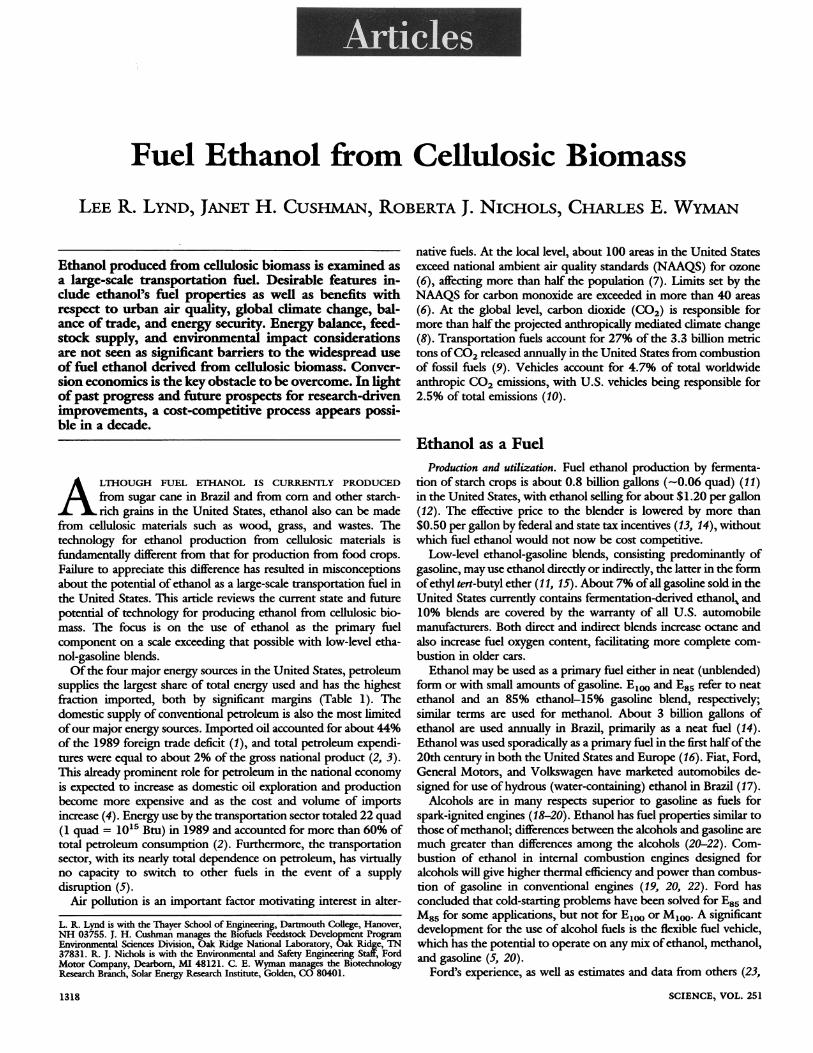
version of cellulosic materials to ethanol; these differ primarily in themethod of hydrolysis and the fermentation system used. Hydrolysisof cellulosic materials can be accomplished with acids or cellulaseenzymes. Projected selling prices for ethanol produced from cellu-lose by acid hydrolysis are currently comparable to those forenzyme-based processes (37). Enzymatic processes are at a muchearlier state of technological maturity; however, in the absence ofunforeseen breakthroughs for acid-based processes, research is likelyto result in enzyme-based processes that are significantly cheaperthan acid-based processes. Steps in conversion of cellulosic biomassinto ethanol by enzymatic processes are depicted in Fig. 1.

Energy balance. The ratio of energy output to energy input, R,may be defined for cellulose-based processes with reference to Fig. 1as

1 + (3*E)R =A+T+C+D+P

(1)

PROCESS EFFLUENTS

Fig. 1. Production of ethanol from cellulosic materials by means ofenzymatic hydrolysis.1320

where E is exported electricity, A is agricultural inputs, T is rawmaterial transport, C is chemical inputs, D is distribution, P is plantamortization, and all energy flows are expressed as fractions of thelower heating value of ethanol. The 1 in the numerator representsethanol and the multiplier ofE reflects the displacement of thermalenergy for conventional power generation. Estimated parametervalues are as follows: E = 0.08 (38),A = 0.15 (Table 2), T = 0.04(39, 40), C = 0.01 (41, 42), D = 0.01 (43), and P = 0.04 (44, 45).Thus, current understanding ofethanol production from cellulose isconsistent with a value of 5 for R. In contrast, R is generally less than1 for corn-based processes without coproduct credits and is approx-imately 1 if coproducts are considered (45, 46).A key factor in considering the energetics of ethanol production

from cellulose is the energy available from residues remaining afterfermentation. It is thought that unfermentable raw material compo-nents, in particular lignin, can be mechanically dewatered andburned to provide 30,000 to 40,000 Btu per gallon of ethanol, anamount in excess of processing energy requirements for currentdesigns with a wood feedstock (38). This excess energy can be used

SCIENCE, VOL. 251

- CarbonConversion --- Energy

Fig. 2. Carbon and energy flows for production and utilization of fuelalcohol from biomass. [Adapted from (53) with permission of HumanaPress, copyright 1989]

to produce electricity in a cogenerative fashion. The thermal effi-ciency (heat ofcombustion ofethanol plus three times the electricityproduction relative to the heat ofcombustion ofthe raw material) ofethanol production from cellulosic materials for a process with highyields is in the range of 45 to 70%, depending on the feedstockcomposition and process configuration.

Global climate change implications. Carbon dioxide productionaccompanies fermentation of the carbohydrate fraction of biomassto ethanol, combustion of unfermentable biomass fractions toprovide process energy, and combustion of fuel ethanol to provideuseful work. The quantity ofCO2 released, however, is precisely thatwhich was previously removed from the atmospheric pool byphotosynthesis in the course of feedstock production. The celluloseethanol fuel cycle thus involves cyclic carbon flow (Fig. 2).

Energy inputs are required at several points to drive the cydedepicted in Fig. 2. Agricultural inputs can be satisfied by either fossilfuels or fuels that do not contribute to CO2 accumulation in theatmosphere, such as ethanol in mobile applications and wood or ligninfor stationary boilers. The same is true for smaller energy and materialinputs associated with equipment depreciation, fertilizer production,and fuel distribution. An indication ofthe contribution offuel optionsto CO2 accumulation is the net carbon produced per unit energy N.For cellulose ethanol, this parameter may be estimated from

N (f-C9(2)wheref is the fraction of energy inputs met by fossil fuels and Cfrepresents CO2 produced per unit energy for fossil energy inputs.Although Cfwill vary for different scenarios, a reasonable value is 80mg of CO2 per kilojoule (47), which is representative for gasoline.With R = 5.0 (see above), Eq. 2 indicates thatN is 16 mg of CO2per kilojoule if only fossil fuels are used for energy inputs, corre-sponding tof = 1. N is 0 for the case in which energy inputs areprovided by sources that do not contribute to CO2 accumulation,however, corresponding tof = 0. Thus, current understanding ofcellulose ethanol technology is consistent with a best case scenarioinvolving no contribution to CO2 accumulation and a worst casescenario resulting in a CO2 contribution about one-fifth that ofgasoline.

Environmental impacts. Airborne emissions, liquid effluents, andsolid wastes from ethanol production processes appear to pose noproblems that cannot be addressed by conventional waste-treatmenttechnology (31, 48). Ethanol is substantially less toxic than metha-nol and gasoline at the same dosage levels (49). The predominant

Fig. 3. Past and project- =ed costs (1988 basis) for " 6ethanol and gasoline. *Past gasoline prices arefrom (2); the range of q,.54future gasoline prices is *s 'Sbased on DOE oil gaso- 'ea Ethanolline price projections ; = 2(4). For ethanol, prices a Gasolineare estimated from pastIresearch and an aggres- - 0sive program for future 1980 1990 2000 2010research. The range X Yearshown arises from as-sumed capital recovery, with the higher values being for a capital recoveryfactor typical of private financing and the lower values being for a capitalrecovery factor more likely for municipal or utility-like finance structures.

toxicity issue associated with ethanol use is intentional consumptionas an intoxicant. Additives such as 3% gasoline, used in Brazil,probably will be added to discourage such consumption.

Conversion economics. As shown in Fig. 3, progress in costreductions has been substantial over the last 10 years, resulting in anapproximately threefold reduction in the projected selling price (37)to $1.35 per gallon in 1988 for technology proven on a laboratoryscale (42). Cost reductions to date stem from minimizing end-product inhibition of cellulase, improved cellulase enzymes andfermentative microorganisms, and improved systems for xylosefermentation. The current cost of producing ethanol from celluloseis the major impediment to utilization of this technology.

Given the cost of representative cellulosic feedstocks (Table 2)and the wholesale selling price required for ethanol to be competi-tive (see above), operating costs, capital recovery, and secondary rawmaterials will have to cost in the range of $0.30 to $0.40 per gallonto be competitive with gasoline prices anticipated in the year 2000.A cost ratio of selling price to primary raw material cost of a factorof 2 is unusually large for a commodity chemical (50), whichsupports our conviction that an economic process is realistic. Thisconviction is further supported by considerations addressed below.Of the ethanol production steps (Fig. 1), only utilities and residue

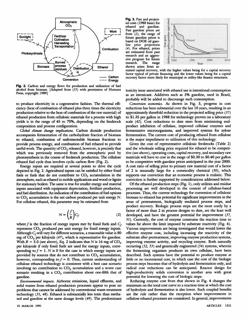
processing are well developed in the context of cellulose-basedprocesses. Thus, the current technology for conversion of cellulosicbiomass to ethanol has potential for significant improvements in theareas of pretreatment, biologically mediated process steps, andproduct recovery. Biologic process steps are the most costly by afactor of more than 2 in process designs to date, are the least welldeveloped, and have the greatest potential for improvement (37,51). Currently, the cost of enzyme constrains the reaction time tovalues far above the limit imposed by substrate reactivity (Fig. 4).Various improvements are being investigated that would lower theeffective enzyme cost, including increasing the reactivity of thesubstrate after pretreatment, improving enzyme production systems,improving enzyme activity, and recycling enzyme. Both naturallyoccurring (52, 53) and genetically engineered (54) systems, whereinthe fermenting organism produces its own cellulase, have beendescribed. Such systems have the potential to produce enzyme atlittle or no incremental cost, in which case the cost of the biologicprocess steps becomes that of hydrolysis and fermentation only, andradical cost reductions can be anticipated. Reactor design forhigh-productivity solids conversion is another area with greatpotential for lowering the cost of biologic steps.Reducing enzyme cost from that shown in Fig. 4 changes the

minimum on the total cost curve to a reaction time at which the costof hydrolysis and fermentation is also lower. Such coupled benefitsare the rule rather than the exception when improvements incellulose ethanol processes are considered. In general, improvements

ARTICLES 132115 MARCH 1991

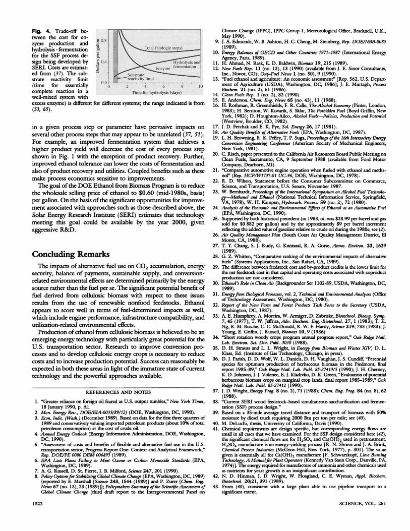
Fig. 4. Trade-off be- -tween the cost for en-zyme production and ° 0.8hydrolysis - fermentation Total (biologic steps)for the SSF process de- *sign being developed by E 0.4 Hydrolysis andSERI. Costs are estimat- Enzyme fermentationed from (37). The sub- : Substratestrate reactivity limit reactivity limit(time for essentially o 2 4 6 8 10complete reaction in a Time for hydrolysis (days)well-mixed system withexcess enzyme) is different for different systems; the range indicated is from(53, 65).

in a given process step or parameter have pervasive impacts onseveral other process steps that may appear to be unrelated (37, 51).For example, an improved fermentation system that achieves ahigher product yield will decrease the cost of every process stepshown in Fig. 1 with the exception of product recovery. Further,improved ethanol tolerance can lower the costs of fermentation andalso of product recovery and utilities. Coupled benefits such as thesemake process economics sensitive to improvements.The goal of the DOE Ethanol from Biomass Program is to reduce

the wholesale selling price of ethanol to $0.60 (mid-1980s, basis)per gallon. On the basis of the significant opportunities for improve-ment associated with approaches such as those described above, theSolar Energy Research Institute (SERI) estimates that technologymeeting this goal could be available by the year 2000, givenaggressive R&D.

Concluding RemarksThe impacts of alternative fuel use on CO2 accumulation, energy

security, balance of payments, sustainable supply, and conversion-related environmental effects are determined primarily by the energysource rather than the fuel per se. The significant potential benefit offuel derived from cellulosic biomass with respect to these issuesresults from the use of renewable nonfood feedstocks. Ethanolappears to score well in terms of fuel-determined impacts as well,which include engine performance, infrastructure compatibility, andutilization-related environmental effects.

Production of ethanol from cellulosic biomass is believed to be anemerging energy technology with particularly great potential for theU.S. transportation sector. Research to improve conversion pro-cesses and to develop cellulosic energy crops is necessary to reducecosts and to increase production potential. Success can reasonably beexpected in both these areas in light of the immature state of currenttechnology and the powerful approaches available.

REFERENCES AND NOTES

1. "Greater reliance on foreign oil feared as U.S. output tumbles," New York Times,18 January 1990, p. Al.

2. Mon. Energy Rev., DOE/EIA-0035(89/12) (DOE, Washington, DC, 1990).3. Econ. Indic. (Wash.) (December 1989). Based on data for the first three quarters of

1989 and conservatively valuing imported petroleum products (about 10% oftotalpetroleum consumption) at the cost of crude oil.

4. Annual Enery Outlook (Energy Information Administration, DOE, Washington,DC, 1990).

5. "Assessment of costs and benefits of flexible and alternative fuel use in the U.S.transportation sector, Progress Report One: Context and Analytical Framework,"Rep. DOEIPE 0080 DE88 006893 (1989).

6. EPA Lists Places Failing to Meet Ozone or Carbon Monoxide Standards (EPA,Washington, DC, 1989).

7. A. G. Russell, D. St. Pierre, J. B. Milford, Science 247, 201 (1990).8. Policy Optionsfor Stabilizing Global Climate Change (EPA, Washington, DC, 1989)

{reported by E. Marshall [Science 243, 1544 (1989)] and P. Zurer [Chem. Eng.News 67 (no. 13), 23 (1989)]}; Policymakers Summary ofthe ScientjficAssessment ofGlobal Climate Change (third draft report to the Intergovernmental Panel on

Climate Change (IPPC), IPPC Group 1, Meteorological Office, Bracknell, U.K.,May 1990).

9. J. A. Edmonds, W. B. Ashton, H. C. Cheng, M. Steinberg, Rep. DOE/NBB-0085(1989).

10. Energy Balances of OECD and Other Countries 1971-1987 (International EnergyAgency, Paris, 1989).

11. H. Ahmad, N. Rask, E. D. Baldwin, Biomass 19, 215 (1989).12. New Fuels Rep. 11 (no. 13), 13 (1990) (available from J. E. Sinor Consultants,

Inc., Niwot, CO); Oxy-Fuel News 1 (no. 50), 9 (1990).13. 'Fuel ethanol and agriculture: An economic assessment" [Rep. 562, U.S. Depart-

ment of Agriculture (USDA), Washington, DC, 1986]; J. E. Murtagh, ProcessBiochem. 21 (no. 2), 61 (1986).

14. Clean Fuels Rep. 1 (no. 2), 82 (1990).15. E. Anderson, Chem. Eng. News 65 (no. 43), 11 (1988).16. H. Rothman, R. Greenshields, F. R. Calle, TheAlcohol Economy (Pinter, London,

1983); H. Bernton, W. Kovarik, S. Sklar, The Forbidden Fuel (Boyd Griffin, NewYork, 1982); D. Houghton-Ailco, Akohol Fuels-Policies, Production and Potential(Westview, Boulder, CO, 1982).

17. J. D. Ferchak and E. K. Pye, Sol. Energy 26, 17 (1981).18. Air Quality Benefits ofAlternative Fuels (EPA, Washington, DC, 1987).19. L. H. Browning, R. K. Pefley, T. P. Suga, Proceedings ofthe 16th Intersociety Energy

Conversion Engineering Conference (American Society of Mechanical Engineers,New York, 1981).

20. C. Risch, paper presented to the California Air Resources Board Public Meeting onClean Fuels, Sacramento, CA, 9 September 1988 (available from Ford MotorCompany, Dearborn, MI).

21. "Comparative automotive engine operation when fueled with ethanol and metha-nol" (Rep. HCP/W1737-01 UC-96, DOE, Washington, DC, 1978).

22. R. D. Wilson, Statement before the Consumer Subcommittee on Commerce,Science, and Transportation, U.S. Senate, November 1987.

23. W. Bernhardt, Proceedings ofthe International Symposium on Akohol Fuel Technolo-gy-Methanol and Ethanol (National Technical Information Service, Springfield,VA, 1978); W. H. Kampen, Hydrocarb. Process. 59 (no. 2), 72 (1980).

24. Analysis ofthe Economic and Environmental Effects ofEthanol as an Automotive Fuel(EPA, Washington, DC, 1990).

25. Supported by both historical precedent (in 1983, oil was $28.99 per barrel and gassold for $0.882 per gallon) and by the approximately $9 per barrel incrementreflecting the added value ofgasoline relative to crude oil during the 1980s; see (2).

26. Air Quality Management Plan (South Coast Air Quality Management District, ElMonte, CA, 1988).

27. T. Y. Chang, S. J. Rudy, G. Kuntasal, R. A. Gorse, Atmos. Environ. 23, 1629(1989).

28. G. Z. Whitten, "Comparative ranking of the environmental impacts of alternativefuels" (Systems Applications, Inc., San Rafael, CA, 1989).

29. The difference between feedstock cost and by-product credits is the lower limit forthe net feedstock cost in that capital and operating costs associated with coproductproduction are not considered.

30. Ethanol's Role in CleanAir (Backgrounder Ser 1102-89, USDA, Washington, DC,1989).

31. Energyfrom Biological Processes, vol. 2, Technical and Environmental Analyses (Officeof Technology Assessment, Washington, DC, 1980).

32. Report of the New Farm and Forest Products Task Force to the Secretary (USDA,Washington, DC, 1987).

33. A. E. Humphrey, A. Moreira, W. Armiger, D. Zabriske, Biotechnol. Bioeng. Symp.7, 45 (1977); T. W. Jeffries, Adv. Biochem. Eng.-Biotechnol. 27, 1 (1983); T. K.Ng, R. M. Busche, C. C. McDonald, R. W. F. Hardy, Science 219, 733 (1983); J.Young, E. Griffin, J. Russell, Biomass 10, 9 (1986).

34. "Short rotation woody crops program annual progress report," Oak Ridge Nati.Lab. Environ. Sci. Div. Publ. 3030 (1988).

35. D. H. Strauss and L. L. Wright, in Energyfrom Biomass and Wastes XIV, D. L.Klass, Ed. (Institute of Gas Technology, Chicago, in press).

36. D. J. Parish, D. D. Wolf, W. L. Daniels, D. H. Vaughan, J. S. Cundiff, "Perennialspecies for optimum production of herbaceous biomass in the Piedmont, finalreport 1985-89," Oak Ridge Natl. Lab. Publ. 85-27413/5 (1990); J. H. Cherney,K. D. Johnson, J. J. Volenec, E. J. Kladivko, D. K. Green, "Evaluation ofpotentialherbaceous biomass crops on marginal crop lands, final report 1985-1989," OakRidge Natl. Lab. Publ. 85-27412 (1990).

37. J. D. Wright, Energy Prog. 8 (no. 2), 71 (1988); Chem. Eng. Prog. 84 (no. 8), 62(1988).

38. "Current SERI wood feedstock-based simultaneous saccharification and fermen-tation (SSF) process design."

39. Based on a 35-mile average travel distance and transport of biomass with 50%moisture by diesel truck requiring 2000 Btu per ton per mile; see (40).

40. M. DeLuchi, thesis, University of California, Davis (1990).41. Chemical requirements are design specific, but corresponding energy flows are

small in all cases that we have examined. For the SSF design considered here (42),the significant chemical flows are for H2S04 and Ca(OH)2 used in pretreatment.H2S04 manufacture is an energy-yielding process [R. N. Shreve and J. A. Brink,Chemical Process Industries (McGraw-Hill, New York, 1977), p. 301]. The valuegiven is essentially all for Ca(OH)2 manufacture [F. Schwarzkopf, Lime BurningTechnology, A Manualfor Plant Operators (Kennedy Van Saun Corp., Danville, PA,1974)]. The energy required for manufacture ofammonia and other chemicals usedas nutrients for yeast growth is an insignificant contribution.

42. N. D. Hinman, J. D. Wright, W. Hoagland, C. E. Wyman, Appl. Biochem.Biotechnol. 20/21, 391 (1989).

43. From (40), consistent with a large plant able to use pipeline transport to asignificant extent.

SCIENCE, VOL. 2511322

44. Value used in (45) for a corn-based ethanol plant; believed to be conservative foran economical cellulose-to-ehanol process.

45. R. S. Chambers, R. A. Herendeen, J. J. Joyce, P. S. Penner,See 206,789 (1979).46. M. A. Johnson, Energy 8, 225 (1983); J. M. Krochta, in Proceedings of the Second

International Conference on Energy Use Management (Pergamon, Elansford, NY,1979), pp. 1956-1963); F. Parisi,Adv. Biochem. Eng.-Biotechnol. 28, 41 (1983);T. Yorifugi, Energy Dev.J. 3, 195 (1981).

47. Based on heat of combustion for petroleum liquids [Basic Pet. Data Book[(American Petroleum Institute, Washington, DC, 1989), vol. 9, no. 3], adding19% for oil recovery, refining, and distribution (40).

48. R. C. Loehr and M. Sengupta, Environ. Sanit. Rev. 16 (1985); E. D. Waits and J.L. Elmore, Environ. Int. 9, 325 (1983).

49. Threshold Limit Values for Chemical Substances and Physical Agents in theWorkman Environment with Intended Changes for 1980s (American Conferenceof Government Industrial Hygienists, Cincinnati, OH, 1980).

50. Hydrocarb. Process. 68 (no. 11), 85 (1989); ibid. 67 (no. 9), 61 (1988).51. L. R Lynd, Appl. Biochem. Biotechnol. 24/25, 695 (1990).52. M. K. Veldhuis, L. M. Christensen, E. I. Fulmer, Ind. Eng. Chem. 28,430 (1936);

T. K. Ng, P. J. Weimer, J. G. Zeikus, Arch. Microbiol. 114, 1 (1977).53. L. R. Lynd, H. E. Grethlein, R. H. Wolkin, Appl. Environ. Microbiol. 55, 3131

(1989).54. J. N. Van Arsdell et al., BiolTechnology 5, 60 (1987); B. Surbriggen, M. J. Bailey,

M. E. Pentrila, K. Poutanen, M. Linko,J. Biotechnol. 13, 267 (1990); M. E.Penttila, P. Lehtovaara, M. Bailey, T. T. Teer, J. K. C. Knowles, Gene 63, 103(1988).

55. National Assessment of Undiscovered Conventional Oil and Gas Resources, Working-Paper (Working pap., U.S. Geological Survey and Minerals Management Service,March 1989); R. A. Kerr, Science 245, 1330 (1989).

56. M. Grathwohl, World Energy Supply (de Gruyter, Berlin, 1982).57. L. R. Lynd, Adv. Biochem. Eng.-Biotechnol. 38, 1 (1989).58. The indicated range is consistent with the evaluation of the DOE Biofuels

Feedstock Development Program [R. D. Perlack and J. W. Ranney, Enery 12 (no.12), 1217 (1987); (35)].

59. S. Kane, J. Reilly, M. LeBlanc, J. Hrubovcak, Agribusiness 5, 505 (1989); FeedSituation and Outlook Report (USDA, FDS-314, Washington, DC, 1990).

60. C. E. Wyman and N. D. Himman,Appl. Biochem. Biotechnol. 24/25, 735 (1990).61. J. D. Ferchak and E. K. Pyc, Sol. Energy 26,9 (1981); J. W. Ranney, L. L. Wright,

P. A. Layton,J. For. 85 (no. 8), 17 (1987); N. Smith and T. J. Corcoran, Am.Chem. Soc. Symp. Ser. 144,433 (1981).

62. G. Marland and A. Turhollow, Oak Ridge Natl. Lab. Environ. Sci. Div. Publ. 3301(1990).

63. Agricultural Resources-Cropland, Water, and Conservation, Situational Outlook andReport (USDA, Washington, DC, 1988).

64. 'Basic Statistics, 1982 National Resources Inventory," USDA Soil Conserv. Serv.Stat. Bull. 756 (1987).

65. H. E. Grethlein, D. C. Allen, A. 0. Converse, Biotechnol. Bioeng. 26,1498 (1984).66. We thank M. DeLuchi, P. Lorang, R. Moorer, and A. Turhollow for useful

discussions and information. Publication 3644, Environmental Sciences Division,Oak Ridge National Laboratory.

Withy Gases Dissolve in Liquids

GERALD L. POLLACK

The thermodynamics and statistical mechanics of solubil-ity are fairly well understood. It is still very difficult,however, to make quantitative predictions of solubilityfor real systems from first principles. The purposes of thisarticle are to present the results of solubility experimentsin some prototype solute-solvent systems, to show howfar they may be understood from molecular first princi-ples, and to discuss some of the things that are stillmissing. The main systems used as examples have theinert gas xenon as solute and some simple organic liquidsas solvents.

A LL GASES DISSOLVE IN ALL LIQUIDS, BUT THE ACTUAL

solubilities range over many orders of magnitude. For inertgases at room temperature, for example, the solubility ofXe

in n-octane, a common hydrocarbon liquid, is 470 times that ofHein water. Gas solubility can vary much more for complex solutes andsolvents. As an example, the solubility of the anesthetic gas

halothane in olive oil is more than 106 times the solubility ofcommon gases in liquid mercury.

Can the solubilities of gases in liquids be quantitatively under-stood from molecular first principles? The question can be general-ized with the help of the Gibbs phase rule, according to whichsystems such as these with two components and two phases havetwo degrees of freedom, such as temperature and pressure. There-fore, the question may be enlarged to include: Can the temperatureand pressure dependence of these solubilities be understood frommolecular first principles?

15 MARCH 1991

One purpose of this article is to discuss how far we can go, using

current experiments and modern theory, in answering these ques-

tions. Also discussed with the same ideas are some applications ofsolubility. Finally, there are some suggestions of what natural next

steps would advance our understanding of the subject.Solubility is an old subject, although most ofthe early interest was

in solubility of solids in water, which is still an important area ofresearch and applications. Aristotle knew that evaporation ofseawa-ter would recover dissolved salts, and there are records of a

systematic study by Pliny the Elder of the relative solubilities ofmany solids in water.

Early quantitative measurements of the solubility of gases, a more

difficult measurement, were made by William Henry (1), as well as

by Cavendish, Priestley, and others. Henry studied the pressure andtemperature dependence of air, H2, N2, 02, and other gases inwater. He discovered, among other things, that 02 is more solublethan N2 in water. This is an early example of the principle that is thebasis of preferential extraction ofone gas from a mixture of gases byuse of a solvent. Since that time, the subject has been actively studiedbecause of its fundamental interest and applications. More recently,extensive contributions to understanding gas solubility have beenmade by Hildebrand and his co-workers and by many others (2, 3).Review articles give comprehensive discussions ofthe subject as wellas results for many solute-gas, solvent-liquid systems (4, 5).Ostwald solubility (L) is an especially useful and also intuitive

measure of gas solubility (6). It is defined as the ratio of theconcentration of gas molecules dissolved at equilibrium in the liquidsolvent to their concentration in the gas phase. In other words, L isthe ratio: (moles of solute per liter of solution)/(moles of solute perliter of gas). We then can write

L = PP2 (1)

where p is the number density and subscripts 1 and 2 stand for,respectively, solvent and solute.

ARTICLES 1323

The author is in the Department of Physics and Astronomy, Michigan State University,East Lansing, MI 48824.