Embed Size (px)
Citation preview
Dynamic Directed Search†
Gabriele Camera Jaehong KimChapman University Chapman UniversityUniversity of Basel
March 20, 2015
Abstract
The directed search model (Peters, 1984) is static; its dynamic extensions typically re-strict strategies, often assuming price or match commitments. We lift such restrictionsto study equilibrium when search can be directed over time, without constraints and atno cost. In equilibrium trade frictions arise endogenously, and price commitments, ifthey do exist, are self-enforcing. In contrast to the typical model, there exists a contin-uum of equilibria that exhibit trade frictions. These equilibria support any price abovethe static price, including monopoly pricing in arbitrarily large markets. Dispersion inposted prices can naturally arise as temporary or permanent phenomenon despite theabsence of pre-existing heterogeneity.
Keywords: frictions, matching, price dispersion, searchJEL: C70, D390, D490, E390
1 Introduction
The directed search model is a decentralized, general-equilibrium trading environ-
ment in which capacity constrained sellers post prices to influence buyers’ search
decisions (Peters, 1984). The game is played in two stages, over the course of one
period. First, prices are posted for everyone to see, then buyers visit a seller of† We thank three anonymous Referees and an anonymous Associate Editor for several helpfulcomments. G. Camera acknowledges partial research support through the NSF grant CCF-1101627. Correspondence address: Gabriele Camera, Economic Science Institute, ChapmanUniversity, One University Dr., Orange, CA 92866; tel.: 714-628-2086; FAX: 714-628-2881; e-mail: [email protected].
1
their choice at no cost, knowing that random rationing is used to meet capacity
constraints. Unlike other search models, search is costless and unrestricted and
trade frictions arise endogenously only if buyers are indifferent where to shop, in
equilibrium. For this reason, the model has been adopted to develop insights in
the analysis of frictional labor and product markets (Burdett et al., 2001; Julien
et al., 2000; Michelacci and Suarez, 2006; Montgomery, 1991; Camera and Selcuk,
2009; Virag, 2010).
The directed search literature has restricted attention to studying equilibrium
when buyers follow symmetric strategies because such symmetry supports equilib-
rium trade frictions (Burdett et al., 2001). A central result is that directed search
equilibrium is unique in small and large markets (Kim and Camera, 2014), and is
inconsistent with posted price dispersion unless there is pre-existing heterogeneity
or costs to make visits. A significant open problem is equilibrium analysis when
market interactions are dynamic. For tractability reasons, the dynamic extensions
in the literature restrict players’ ability to fully exploit the temporal structure of
the game. Typical assumptions include history-independent strategies, price com-
mitments or match commitments, exogenous separation shocks, etc.1 This study
characterizes equilibria when these restrictions are lifted. The exercise is mean-
ingful for two reasons. It fills an important gap regarding the type of equilibria
that exist under dynamic directed search; for example, one would expect to see1See, for instance, Acemoglu and Shimer (1999); Albrecht et al. (2006); Julien et al. (2000);Galenianos and Kircher (2009). Essentially, these assumptions eliminate the need to considerhow others would modify their strategies in the continuation game as a reaction to informationabout deviations. For example, with price commitments a seller who advertises a price belowequilibrium does not have to worry that her competitors might react by sharply cutting theirprices for the foreseeable future.
2
many other equilibria—exhibiting some degree of price collusion perhaps—when
prices are repeatedly posted for everyone to see (e.g., Cason and Noussair, 2007;
Anbarci and Feltovich, 2013). In addition, understanding how the directed search
model performs when players can fully exploit the temporal structure of the game
can open up its use to a richer set of applications compared to those that can be
handled with the standard, static model.
We report that, unlike the typical model, a rich set of equilibria emerges that
supports endogenous trade frictions. In these equilibria, match selection and du-
ration are both endogenous and price commitments, if they do exist, are self-
enforcing. There always exists a continuum of equilibria in which sellers post
an identical price that lies in between the static Nash equilibrium price and the
monopoly price. The size of the equilibrium set depends on market tightness and
discounting. These “collusive” equilibria are supported by the sellers’ threat to
play the static Nash equilibrium if any competitor cuts their price. The threat
is credible because posted prices are public in the model, and static pricing is
always an equilibrium of the dynamic game, but is the one that generates the
lowest revenues. As a consequence, we obtain a result that mirrors the one in
Diamond (1971); monopoly prices can be supported in markets where many sell-
ers compete for a few buyers, even if buyers’ search is costless and unrestricted
by external matching processes. Importantly, this result holds in arbitrarily large
markets. On the other hand, buyers cannot induce sellers to cut prices below
the static Nash value. Buyers cannot credibly threaten to lower a seller’s payoff
by modifying their search behavior, punishing a seller by shopping elsewhere, for
3
example.
Another unique result is the existence of a continuum of equilibria that sup-
port posted price dispersion and trade frictions. These outcomes arise despite the
absence of pre-existing heterogeneity or search costs, and can emerge as either
a stable or a temporary phenomenon. In equilibrium, sellers who post different
prices earn different payoffs because they all attract some buyers who, in equi-
librium, are indifferent where they shop. These outcomes can be supported as
equilibria because sellers can exploit the dynamic nature of the game reacting to
undesirable changes in the distribution of posted prices by aggressively cutting
prices in the continuation game. This finding contrasts with what is observed in
the typical model, which does not admit trade frictions and dispersion in posted
prices unless markets can be segmented by search costs or productivity differen-
tials. For example, Montgomery (1991); Galenianos et al. (2011) study equilibria
characterized by heterogeneous posted wages that are supported by exogenously
different productivities. Burdett et al. (2001) discuss equilibria with dispersion in
posted price that do not support trade frictions and, in fact, require buyers’ per-
fect coordination in search strategies. Price-dispersion equilibria with endogenous
trade frictions are discussed in Camera and Selcuk (2009), but dispersion in that
study involves realized prices that can be renegotiated after sellers meet buyers.
Finally, posted wage dispersion arises in Kircher (2009) as the market splits into
separated sub-markets when buyers can pay a cost to simultaneously visit multiple
markets.
The model is applicable to a variety of retail markets for homogeneous goods
4
in which sellers compete in prices. If prices are transparent, then sellers can tacitly
collude by regularly monitoring each other’s price. A typical example is offered
by the industry for retail gasoline, where gas station operators can coordinate on
setting prices above the competitive level by threatening price wars. For example,
consider the study in Slade (1992); it found evidence of tacit collusion among
gas station operators, with stable and uniform prices during prolonged periods
of normal demand (although admittedly, in that model capacity constraints do
not play as crucial a role as in directed search). But one can think of other
homogeneous product markets in which prices are transparent as in retail gasoline
markets, such as retail consumer electronics or airline seats. Yet again, the model is
applicable to labor markets in which firms compete in wages—the typical markets
considered in the directed search literature (e.g., Albrecht et al., 2006; Julien et
al., 2000).
The paper proceeds as follows. Section 2 presents the model and lays out
some notation. Section 3 offers some preliminaries involving properties of prices
in the static game, which are necessary to derive the results for the dynamic game,
presented in Section 4. Section 5 concludes.
2 The model
The model follows the one in Peters (1984). In each period t = 1, 2, . . . there
is a constant population of I = {1, . . . , I} anonymous and identical buyers and
J = {1, . . . , J} homogeneous sellers each of whom has an indivisible good to sell
5
in each period. All players are infinitely lived.
In each period t seller j can choose to post a price ptj. By posting price ptj
seller j commits to sell at that price in period t to any buyer. However, sellers
cannot commit to any future price. Trading at price ptj generates utility v(ptj) to
the buyer of the good, with v′ < 0. Given the one-to-one relationship between
prices and utilities, for convenience we will think of seller j as promising utility
vtj := v(ptj) to any buyer.2 We will thus interchangeably use the phrases “post
a higher (lower) price” or “promise a lower (higher) utility,” when no confusion
arises. It is assumed that vtj ∈ [v, v], where 0 ≤ v < v. Fixing t, denote the action
profile of sellers for the period by vt = (vt1, . . . , vtJ) ∈ XJ [v, v]; also, let vt−j denote
vt where the jth component is removed.
In each period t buyers choose to visit one seller, based on the utility promised
by sellers, in the period. In symmetric equilibrium, the choice of a buyer for a
period t is a probability distribution over sellers (πt1, . . . , πtJ). In any period t,
given πtj and vtj, seller j’s payoff function for the period is M(πtj)φ(vtj) where the
functionM(πtj) denotes the probability that seller j trades and the seller’s utility
function φ : [v, v] → R is concave, decreasing, with φ(v) = 0. Sellers discount
future utility geometrically at rate β ∈ (0, 1).
If a buyer visits seller j in period t, the buyer’s payoff is H(πtj)vtj, where the
functionH(πtj) denotes the probability that the buyer trades with seller j, in which
case the buyer’s utility is vtj. Buyers discount future utility geometrically, at rate
βb ∈ (0, 1). Market participants observe all promised utilities and the realization2Hence, “promised utility” here refers to the utility earned ex-post by a buyer who trades withseller j, not to be confused with the utility a buyer can expect ex-ante from visiting seller j.
6
of demand in their meeting. Sellers’ identities are also observable.
3 Preliminaries: the static game
To start, we report some results for the static game, which will be useful to
study the repeated game. Consider an outcome in which buyers adopt symmetric
strategies. Let qi(I, π) denote the probability that the generic seller j meets i =
1, . . . , I buyers when each of I buyers chooses the seller with probability π. Let
ρ(i) = 1i
denote a random rationing rule at a seller who has been visited by i
buyers. We can thus define
M(π) :=I∑i=1
qi(I, π) = 1− (1− π)I ,
H(π) :=I−1∑i=0
qi(I − 1, π)ρ(i+ 1) = M(π)Iπ
= 1I
I−1∑i=0
(1− π)i.
The function M(π) denotes the unconditional probability that a seller trades,
given that all buyers visit the seller with probability π. The function H(π) is
the conditional probability that a buyer trades conditional on visiting a seller,
when every other buyer visits that same seller with probability π. In symmetric
equilibrium, vj = v, πj = 1J
for all j, and M( 1J
) = 1−(1− 1
J
)I.
We start by defining visiting probabilities in a symmetric Nash equilibrium of
the static game.
Definition 1. Given v := (v1, v2, . . . , vJ), the distribution of probabilities π(v) in
7
symmetric equilibrium must satisfy ∑j∈J
πj(v) = 1; if πj(v) > 0 for j ∈ J , then
H(πj(v))vj = maxk∈JH(πk(v))vk.
Since buyers are free to visit any seller, in symmetric equilibrium we need
H(πj)vj = H(πl)vl ≥ H(0)vk, for all πj, πl > 0, πk = 0. Because we focus on a
strongly symmetric equilibrium (as in the literature), let v−j denote the identical
strategy of the competitors of seller j. With a small abuse in notation, we may
also use πj(vj, v−j) instead of πj(v).
Proposition 1. Consider a static game. Fix v−j = x > 0. There is a unique
vj(x) ∈ [v, v] that maximizes seller j’s profit
Φ(vj, x) =M(πj(vj, x))φ(vj),
where Φ(vj, x) and Φ(vj(x), x) are both decreasing in x. In addition, if vj(x) = x
for a unique x = v∗ ∈ (0, v), then we have
• If x < v∗, then vj(x) > x;
• If x > v∗, then vj(x) < x.
The proof is in the Appendix. It is well-known that the symmetric equilibrium
v in the static game with homogeneous sellers is unique: vj = v∗ for all j with
0 < v∗ < v. Yet, Proposition 1 is helpful because it tells us how a seller would
optimally react if his competitors would all collude on promising an identical
utility x that is different from the equilibrium level v∗. The message is that a
8
seller should react to competitors who all promise x > v∗ by promising a utility
below x; instead, if all competitors promise utility x < v∗, then the seller should
promise a utility above x.
This result is crucial when we consider the possibility of price collusion—or,
equivalently, collusion in promised utilities—in the dynamic game. In the static
game, instead, there cannot be collusion and the intuition is as follows: If every
competitor attempted to increase their profits by promising a lower utility v−j =
x < v∗ (i.e., posting a higher price), then a rational seller should promise a utility
vj(x) > x above her competitors’ (the converse also holds). This is the central
reason why price collusion cannot be sustained in the static game. Things are
different once the directed search model is extended to a dynamic environment:
here, sellers might wish to react to a deviation by changing their behavior in (part
of) the continuation game. The section that follows shows how this can be done.
4 Price collusion in small and large markets
In this section we study sequential equilibrium in the dynamic model. In every
period, buyers are free to visit any seller and sellers are free to promise any utility,
i.e., there is neither commitment to prices nor to meetings. For the moment,
consider outcomes that are stationary and symmetric in the sense discussed before;
all sellers behave identically and all buyers behave identically. In such equilibria,
the promised utilities vj and the buyers’ choices πj must be time-invariant. In
addition, vj = v and πj = 1/J for all j ∈ J in each period.
9
We start by defining two intuitive strategies for a generic seller j ∈ J .
Definition 2 (Static Nash). In each period the seller promises vj = v∗, i.e., the
strategy is (v∗, v∗, . . .).
The static Nash strategy is an open loop strategy. The seller ignores infor-
mation on past pricing behaviors—as if it was not observed—and mechanically
repeats static play, day in and day out. Such mechanical behavior has been con-
sidered, for instance, in the dynamic direct search extensions of Julien et al. (2000)
and Albrecht et al. (2006). The static Nash strategy supports a sequential sym-
metric equilibrium because playing v∗ is always the best response to play of v∗ by
every other competitor. If static Nash is the strategy adopted, then the seller’s
payoff Π∗ can be recursively defined by Π∗ =M( 1J
)φ(v∗) + βΠ∗, so that
Π∗ = 11− βM( 1
J)φ(v∗).
Definition 3 (Collusive strategy). Consider a seller j. In period t = 1, the seller
promises v1j = vc. In all t ≥ 2, the seller is in one of two states: colluding
or punishing. A colluding seller promises vc for the period; a punishing seller
promises v∗. If the seller is colluding in t, then: (i) If vti = vc for all i ∈ J , then
the seller keeps colluding in t + 1; (ii) otherwise, the seller permanently switches
to punishing.
Such a strategy is typical for models of cooperation in repeated games and is
composed of two parts: a rule of desirable behavior (promises vc) and a rule of
punishment (promises v∗ forever) that is selected only if a departure from desirable
10

behavior is observed. Collusion can be supported by the threat of an immediate,
permanent and market-wide switch to static Nash play because in the directed
search model prices are publicly posted. If vc < v∗, then we interpret vc as a
collusive promised utility—equivalently, as price collusion.
If the collusive strategy is a social norm, i.e., if all sellers adopt it, then
Πc := 11− βM( 1
J)φ(vc)
denotes the seller’s payoff from colluding. We now present a Folk Theorem-type
result for the dynamic direct search model.
Theorem 2. The collusive strategy supports a continuum of symmetric stationary
sequential equilibria vc ∈ [v, v∗]. In particular,
1. vc = v∗ is always an equilibrium;
2. for vc ∈ [v, v∗), there exists β(vc) < 1 such that if β ≥ β(vc), then the
collusive strategy is an equilibrium;
Corollary 3. vc > v∗ is never an equilibrium under the collusive strategy.
Proof of Theorem 2. We must consider the choices of a deviant seller in three
cases, which depend on whether vc is zero, or it is positive and below or above v∗.
Case 1: 0 < vc ≤ v∗.
Note that vc = v∗ is always the best response to v∗, in each period.
Now consider 0 < vc < v∗. We start by discussing choices in equilibrium. Let
vd(vc) denote the best possible deviation in an equilibrium where vc is the collusive
11
promised utility, and let πd(vc) denote the corresponding probability to visit the
deviant seller. We omit the argument vc when it is understood.
A seller does not defect in equilibrium if
Πc ≥ Πd :=M(πd)φ(vd) + βΠ∗ =M(πd)φ(vd) + β
1− βM( 1J
)φ(v∗).
Using the definition for Πc, the above inequality holds if
β ≥ βc :=M(πd)φ(vd)−M( 1
J)φ(vc)
M(πd)φ(vd)−M( 1J
)φ(v∗) .
We have βc < 1 for vc < v∗, because φ(vc) > φ(v∗) by the properties of φ.
To find the best possible deviation vd(vc), we must find the value vd that
maximizes Πd, i.e., the value that maximizes M(πd)φ(vd), because Π∗ is given.
Because we focus on strongly symmetric equilibrium, denote by v−j the identical
strategy of all sellers other than seller j. From Proposition 1, we know that the
maximizer vd(vc) is unique for all v−j = vc < v∗ and it is such that vd(vc) > vc.
More specifically, the best deviation vd(vc) is a solution to
maxvjM(πj(vj, vc))φ(vj) s.t. H(πj)vj = H(1−πj
J−1 )vc,
where the constraint ensures that buyers are indifferent (= indifference constraint).
The first order condition for an interior solution is
M′(πj)∂πj∂vj
φ(vj) +M(πj)φ′(vj) = 0.
12
Using the indifference constraint, we have
∂πj∂vj
= − (J − 1)H(πj)H′(1−πj
J−1 )vc + (J − 1)H′(πj)vj.
A standard result is that M(πj) = IπjH(πj), which we can use to rearrange the
first order condition together with ∂πj∂vj
. We obtain that if there exists an interior
solution vd(vc), then vd(vc) =H(1−πd
J−1 )vcH(πd)
(from the indifference constraint) and
πj = πd ∈ (0, 1), where πd must solve the rearranged first order condition
(J − 1)M′(πd)φ(H(1−πd
J−1 )vcH(πd)
)− Iπdφ′
(H(1−πd
J−1 )vcH(πd)
)
×[H′(1−πd
J−1 )vc + (J − 1)H′(πd)H(1−πd
J−1 )vcH(πd)
]= 0.
Otherwise, we have a corner solution πj = 1, with vd = H(0)vcH(1) which is when the
constraint binds, so that the deviant seller gets all buyers.
Finally, consider the optimality of playing v∗ out of equilibrium. Out of equi-
librium, v∗ maximizes the sellers’ payoff when every other seller follows the pun-
ishment prescribed by the collusive strategy, i.e., v−j = v∗. Hence it is never
optimal to play vj 6= v∗ out of equilibrium. The proof is by contradiction. Sup-
pose vj = v 6= v∗ is optimal out of equilibrium. Then we must have
Π∗ =M( 1J
)φ(v∗) + βΠ∗ ≤M(π(v, v∗))φ(v) + βΠ∗.
But v∗ is the unique maximizer in static game, when v−j = v∗ (Proposition 1), so
M( 1J
)φ(v∗) >M(π(v, v∗))φ(v), which gives us the desired contradiction.
13
Case 2: vc = 0.
This case differs from the previous one because there is no maximizer vd(vc) due
to a discontinuity of πj(vj, 0). This has been discussed in Proposition 1. Hence,
suppose that the deviant seller sets vj = ε > 0 when v−j = 0. In this case πj = 1.
Thus the payoff to the deviant seller is
Πd(ε) =M(1)φ(ε) + βΠ∗.
It is suboptimal to deviate in equilibrium, if
Πc > limε→0
Πd(ε) =M(1)φ(0) + β
1− βM( 1J
)φ(v∗),
which can be rearranged as β > β0, where
β0 :=M(1)φ(0)−M( 1
J)φ(0)
M(1)φ(0)−M( 1J
)φ(v∗) .
We have β0 < 1, because φ(0) > φ(v∗). Finally, define
β(vc) =
β0, if vc = 0
βc, if vc > 0.
Case 3: vc > v∗.
We will show that this cannot be an equilibrium, by means of a contradiction. If
in equilibrium a seller deviates to vd(vc), then the deviant seller is visited with
14
probability πd by any buyer in the period when the deviation takes place. The
deviant seller plays v∗ in all subsequent periods; hence from then on the seller is
visited with probability 1J
. Since vc > v∗, and vd(vc) is the maximizer, we have
M( 1J
)φ(vc) < min{M(πd)φ(vd(vc)),M( 1J
)φ(v∗)}. This implies
Πc =M( 1J
)φ(vc) + βΠc <M(πd)φ(vd(vc)) + βΠ∗,
because Πc =M( 1
J)φ(vc)
1− β < Π∗ =M( 1
J)φ(v∗)
1− β . Hence, if vc > v∗, then there is a
profitable deviation vd(vc), which gives us the desired contradiction.
Corollary 4. Fix the number of buyers I = Jr with r > 0. A version of Theorem
2 holds in the limit as J →∞.3
The lesson is that in the dynamic directed search model, surplus can be easily
redistributed from buyers to sellers because directed search is based on public
monitoring of prices. Consequently, sellers who are sufficiently patient can collude
on any price higher than the static Nash price, independent of market tightness.
This is a unique result because market tightness is the central determinant of
prices in the typical directed search model.
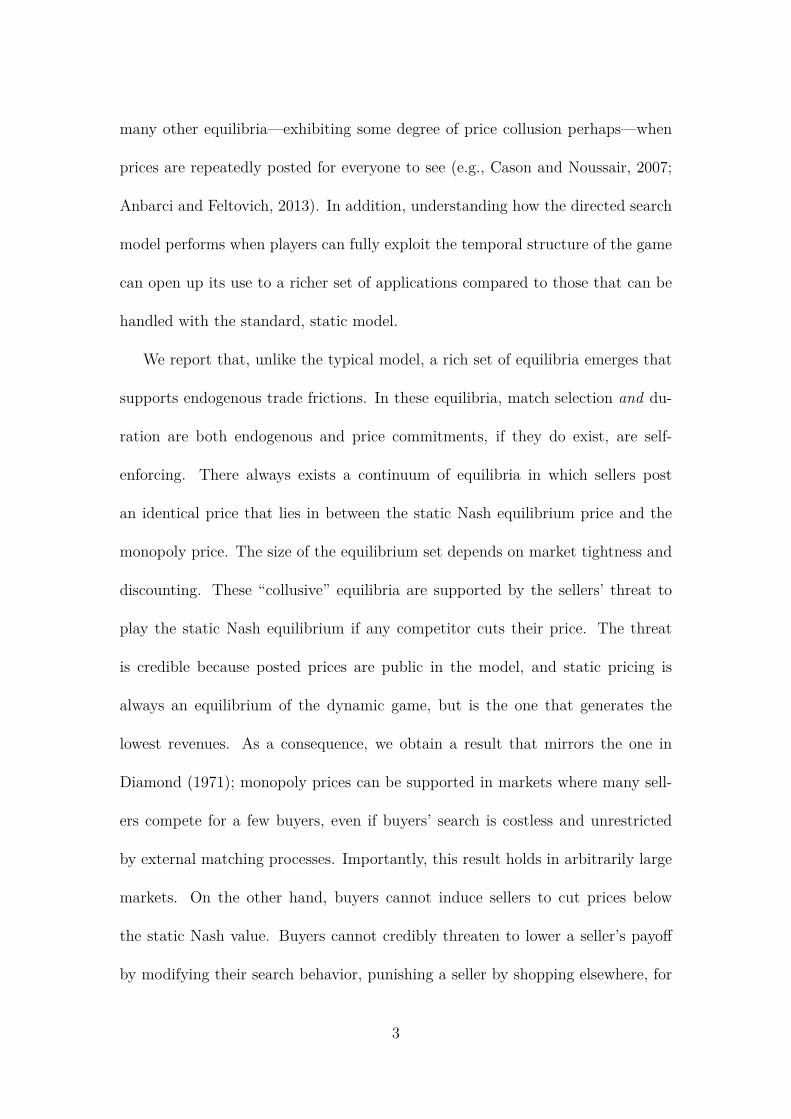
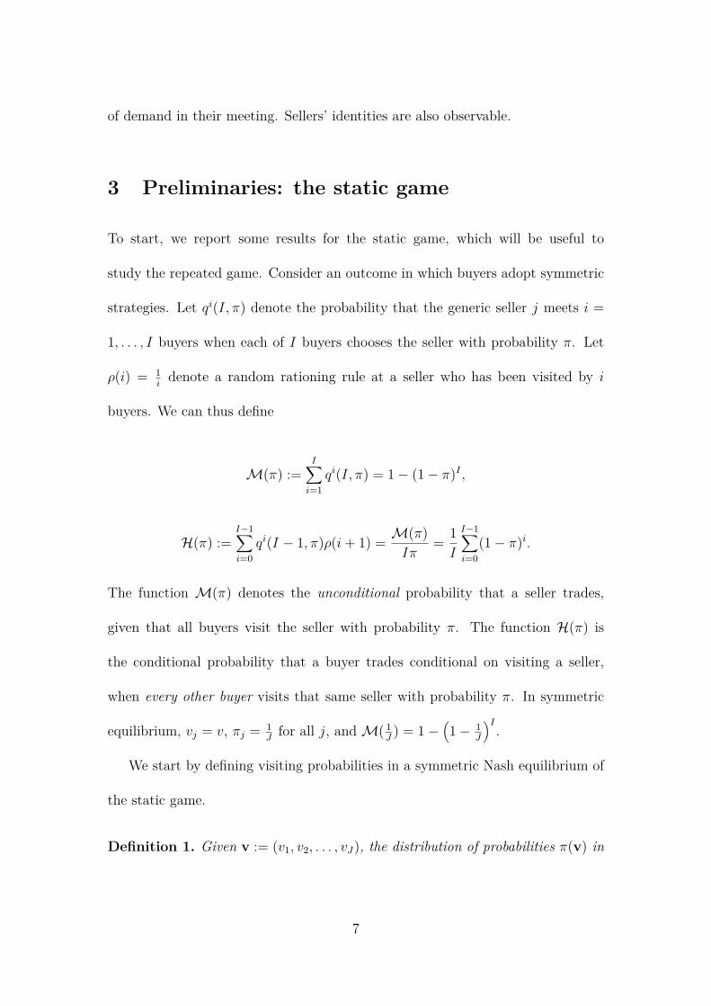
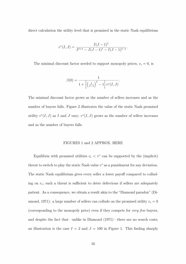
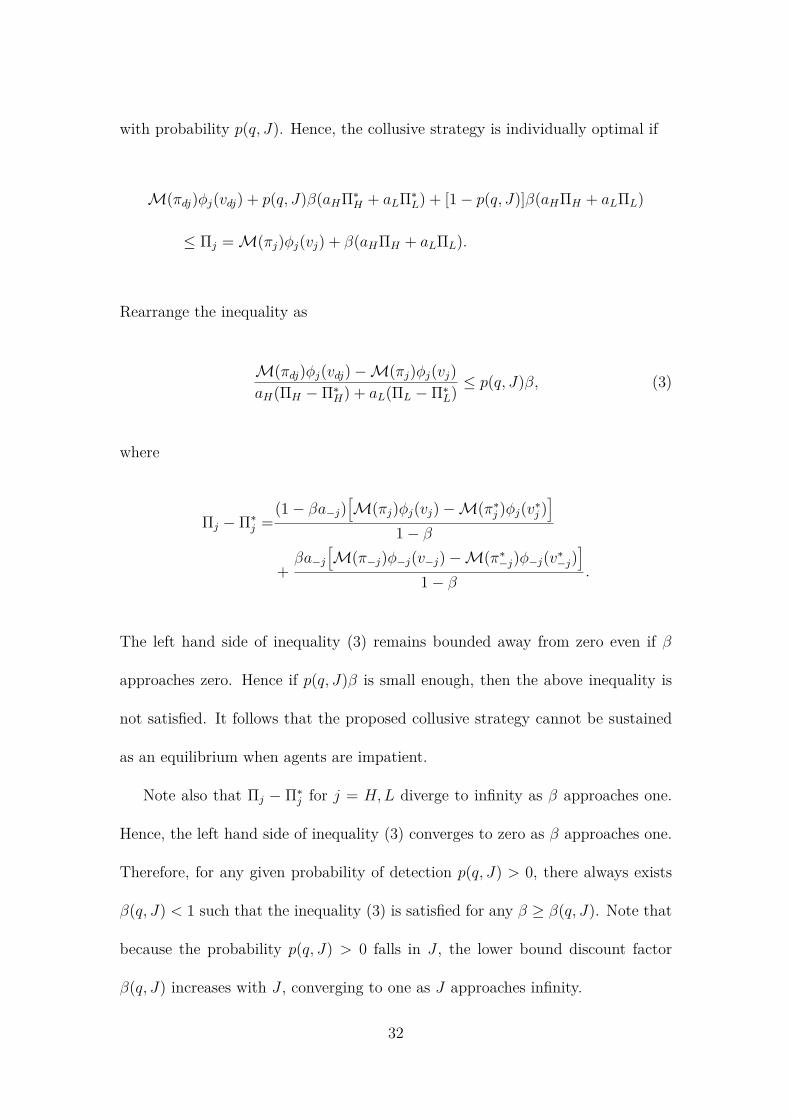
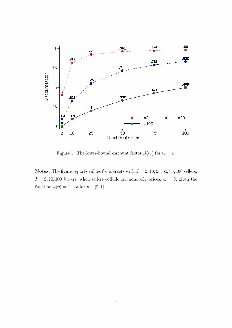
An illustration of Theorem 2 is provided in Figures 1-2. Figure 1 illustrates
the mapping between the lower-bound discount factor β(vc), for markets where
the number of sellers and the number of buyers vary between 2 and 100, when
sellers collude on monopoly prices, vc = 0 and φ(v) = 1 − v for v ∈ [0, 1]. In
symmetric equilibrium πj = 1/J for all sellers j = 1, . . . , J and we obtain by3The proof of Corollary 4 mirrors the one for small markets. It is contained in an additionalappendix available upon request.
15
direct calculation the utility level that is promised in the static Nash equilibrium
v∗(I, J) = I(J − 1)IJ I+1 − J(J − 1)I − I(J − 1)I−1 .
The minimal discount factor needed to support monopoly prices, vc = 0, is
β(0) = 1
1 +[(
JJ−1
)I− 1
]v∗(I, J)
.
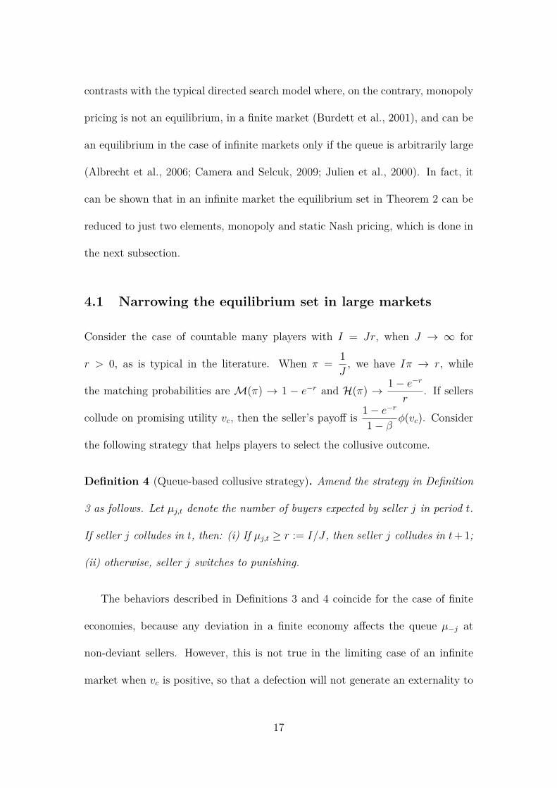
The minimal discount factor grows as the number of sellers increases and as the
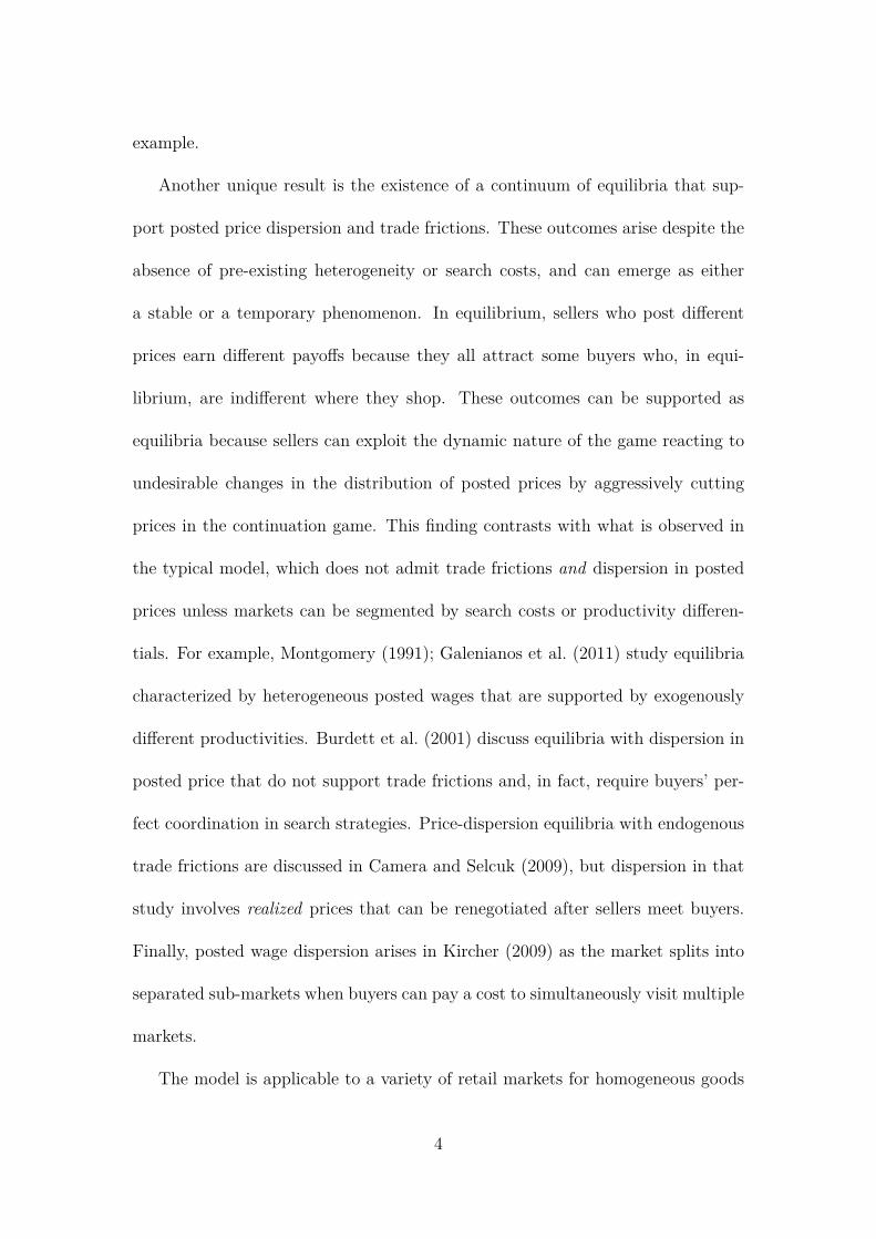
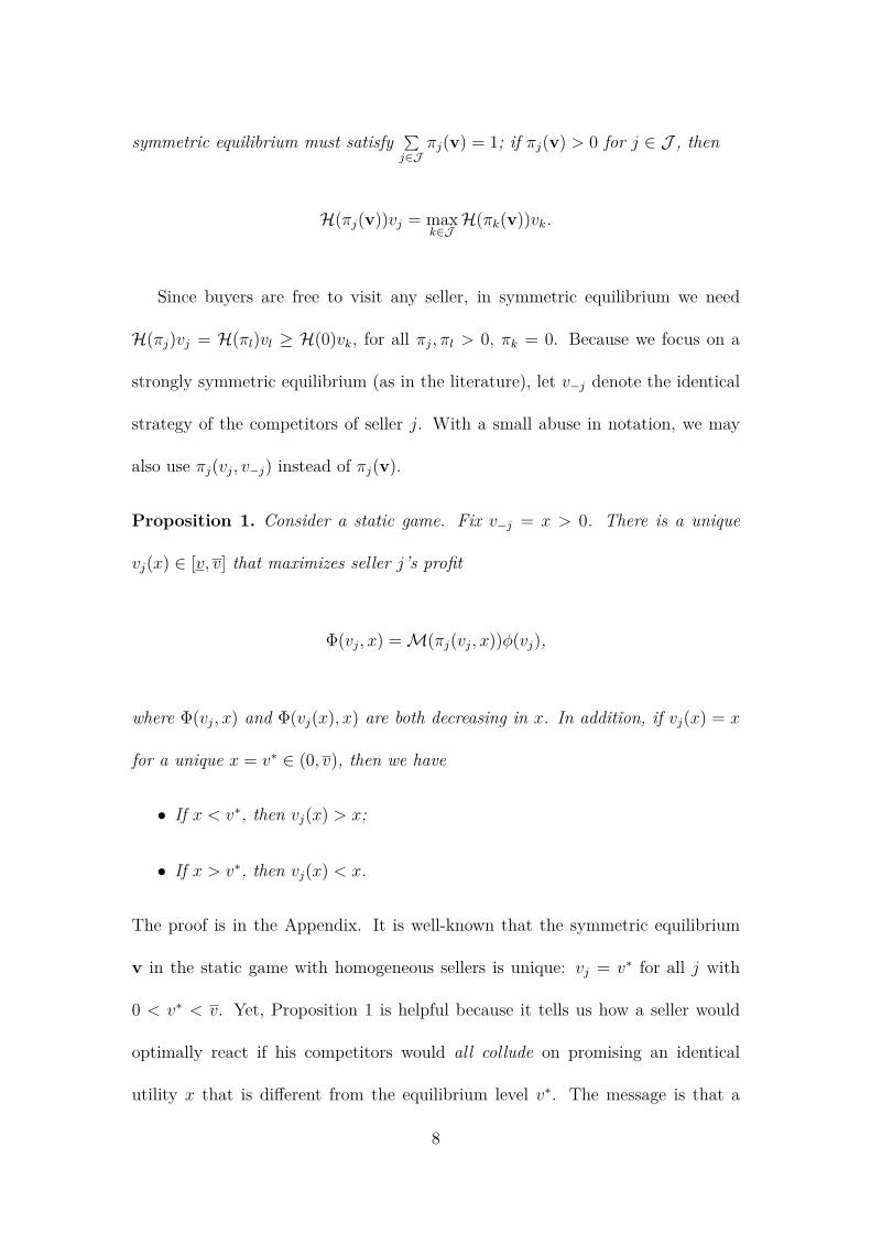
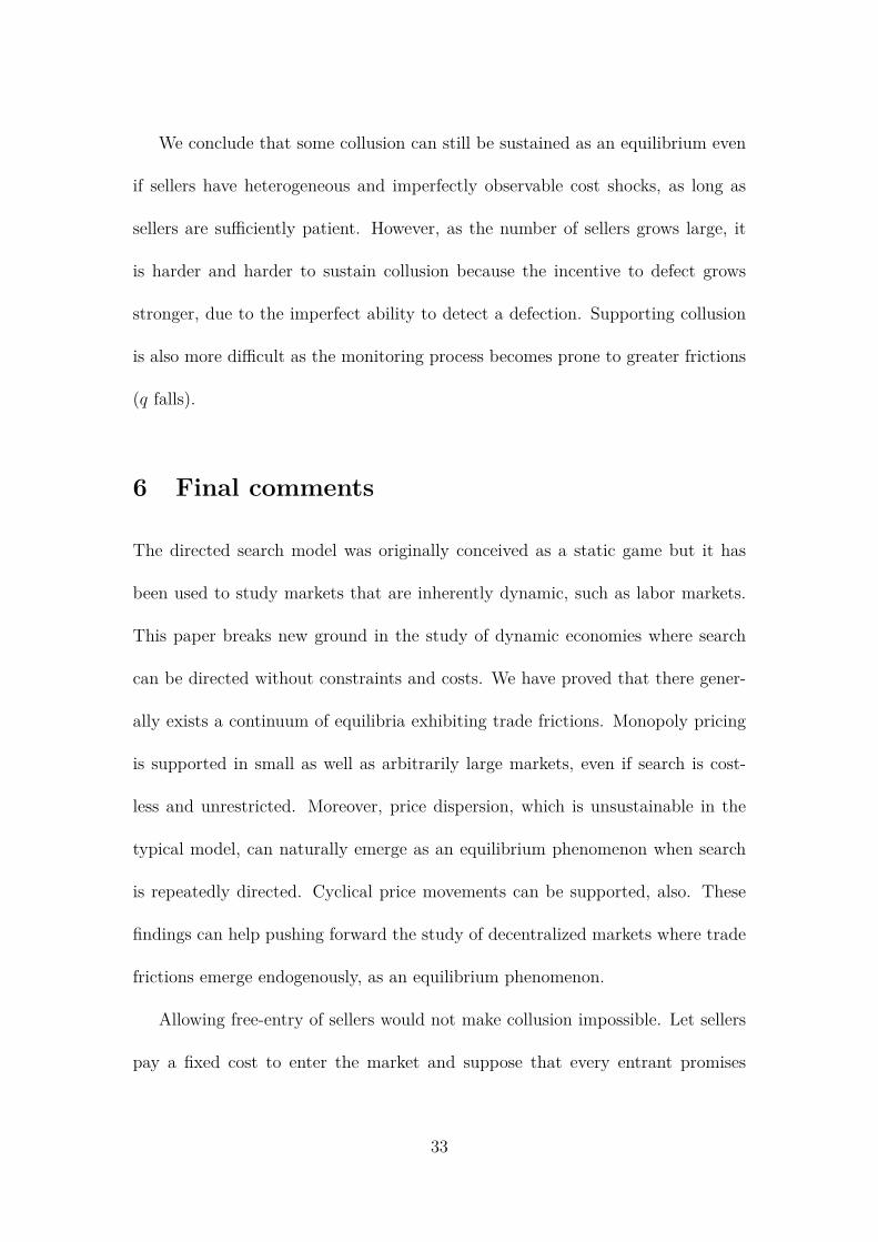
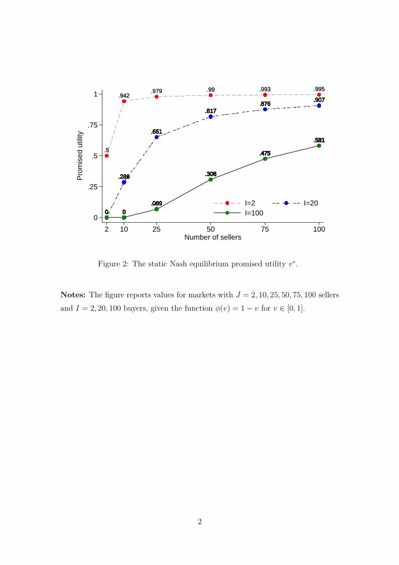
number of buyers falls. Figure 2 illustrates the value of the static Nash promised
utility v∗(I, J) as I and J vary; v∗(I, J) grows as the number of sellers increases
and as the number of buyers falls.
FIGURES 1 and 2 APPROX. HERE
Equilibria with promised utilities vc < v∗ can be supported by the (implicit)
threat to switch to play the static Nash value v∗ as a punishment for any deviation.
The static Nash equilibrium gives every seller a lower payoff compared to collud-
ing on vc; such a threat is sufficient to deter defections if sellers are adequately
patient. As a consequence, we obtain a result akin to the “Diamond paradox” (Di-
amond, 1971): a large number of sellers can collude on the promised utility vc = 0
(corresponding to the monopoly price) even if they compete for very few buyers,
and despite the fact that—unlike in Diamond (1971)—there are no search costs;
an illustration is the case I = 2 and J = 100 in Figure 1. This finding sharply
16
contrasts with the typical directed search model where, on the contrary, monopoly
pricing is not an equilibrium, in a finite market (Burdett et al., 2001), and can be
an equilibrium in the case of infinite markets only if the queue is arbitrarily large
(Albrecht et al., 2006; Camera and Selcuk, 2009; Julien et al., 2000). In fact, it
can be shown that in an infinite market the equilibrium set in Theorem 2 can be
reduced to just two elements, monopoly and static Nash pricing, which is done in
the next subsection.
4.1 Narrowing the equilibrium set in large markets
Consider the case of countable many players with I = Jr, when J → ∞ for
r > 0, as is typical in the literature. When π = 1J
, we have Iπ → r, while
the matching probabilities are M(π) → 1 − e−r and H(π) → 1− e−rr
. If sellers
collude on promising utility vc, then the seller’s payoff is 1− e−r1− β φ(vc). Consider
the following strategy that helps players to select the collusive outcome.
Definition 4 (Queue-based collusive strategy). Amend the strategy in Definition
3 as follows. Let µj,t denote the number of buyers expected by seller j in period t.
If seller j colludes in t, then: (i) If µj,t ≥ r := I/J , then seller j colludes in t+ 1;
(ii) otherwise, seller j switches to punishing.
The behaviors described in Definitions 3 and 4 coincide for the case of finite
economies, because any deviation in a finite economy affects the queue µ−j at
non-deviant sellers. However, this is not true in the limiting case of an infinite
market when vc is positive, so that a defection will not generate an externality to
17
non-deviant sellers. This characteristic can be exploited by sellers to collude as if
they were monopolists, as we demonstrate next.
Proposition 5. Let 0 ≤ v < v. The strategy in Definition 4 supports two symmet-
ric stationary sequential equilibria: vc = v∗, always, and vc = 0 if β ∈ [β(0), 1).
The proof is in the Appendix. As the market grows infinitely large, a single
deviation from vc > 0 does not affect the payoffs of non-deviant sellers. This
is so, because setting vj 6= vc > 0 cannot change the distribution of buyers at
non-deviant sellers, i.e., there is no change in the queue, µ−j = r. However, if
vc = 0, then a single deviation vj > 0 can soak up infinitely many buyers away
from non-deviant sellers, simply because buyers’ payoff is 0. This is true in a finite
market and so it holds true in the limit as a market grows infinitely large. In this
case, a single deviation to vj 6= 0 changes the queue at all non-deviant sellers from
µ−j = r to µ−j < r (possibly 0). Consequently, a single deviation from vc = 0
triggers the punishment phase; if players are sufficiently patient, this will deter
any deviation.
4.2 Can prices fall below the static equilibrium price?
There are many punishment strategies that let sellers obtain payoffs above the
static Nash, apart from the strategy in Definition 3. For instance, sellers can
resort to a penal code-type of punishment, whereby sellers revert to collusion after
a sufficiently long punishment spell. But, the promised utility cannot end up above
the static value. There are two reasons for this finding. First, Proposition 1 has
demonstrated that there is always an incentive to deviate from vc > v∗ because
18
there exists a best deviation vd(vc) < vc and a corresponding visiting strategy
πd such that M(πd)φ(vd)1− β >
M( 1J
)φ(vc)1− β . Second, competitors never have an
incentive to punish the best deviation vd(vc) < vc asM(1−πd
J−1 )φ(vc)1− β >
M( 1J
)φ(vc)1− β ,
i.e., the deviation is profitable to the deviator and his competitors: it generates
a positive externality for all non-deviant sellers because their expected demand
increases. As such, vc > v∗ cannot be a symmetric equilibrium because sellers
have no reason to sustain it. The open question is: could buyers exploit the
dynamic structure of the game to motivate sellers to promise utilities above the
static Nash value v∗? For example, could buyers successfully threaten to ostracize
sellers who deviate from promising a utility vc > v∗?
This threat is not credible since buyers do not have a way to commit to carrying
it out (and sellers have no incentive to punish a deviation, as seen above). To see
why this is so, suppose that buyers punish a seller who deviates to 0 < vd <
vc by shopping more frequently elsewhere, forever. That is, buyers collectively
punish the deviant seller with 0 ≤ πd < πd forever; this may not be optimal for
buyers. Given permanent punishment, the deviant seller promises vd utility in
all subsequent periods, hence his payoff is M(πd)φ(vd)1− β . But πd < πd is never
optimal for buyers, i.e., they will not ostracize a deviant seller who promises
positive utility. Buyers can earn a greater payoff by visiting the deviant sellers since
H(πd)vd > H(
1−πd
J−1
)vc; this follows from the symmetric equilibrium indifference
condition H(πd)vd = H(1−πd
J−1 )vc and the monotonicity of the matching function
H. Hence, an argument similar to the above demonstrates that vc > v∗ cannot be
an equilibrium; a seller can improve his payoff by deviating by optimally choosing
19
some 0 < vd < vc.
5 Frictional equilibria with price dispersion
The directed search model with homogeneous players does not support equilibrium
frictions and dispersion in posted prices or, equivalently, in promised utilities. It
supports either one, or the other separately, unless there are some exogenous
heterogeneity elements, as in Montgomery (1991) and Kim and Camera (2014).
For example, in Burdett et al. (2001) dispersion in posted prices may occur if
buyers coordinate their actions and choose not to direct their search at random.
This section demonstrates that equilibrium (posted) price dispersion and trade
frictions naturally arise when market participants can interact repeatedly over
time. We will show that the degree of price heterogeneity may be time-invariant
or not.
To prove this unique finding, we take two steps. To develop intuition, we first
show that small degrees of price dispersion are compatible with symmetric equilib-
rium if sellers can publicly observe the outcome of a random pricing mechanism.
The mechanism randomizes prices to be posted over a small, pre-specified interval.
We show that this is never an equilibrium in the static model, but it can be an
equilibrium when sellers interact repeatedly. In this equilibrium sellers choose to
ignore price variations in the market, as long as they are sufficiently small and the
mean price is sufficiently high. We call these “small dispersion” equilibria.
Then, we remove this public randomization device entirely. In an additional
20
section, we show that significant degrees of price dispersion can be sustained in
equilibrium when sellers behave asymmetrically. However, buyers still play sym-
metric strategies, optimally choosing to randomize their visits across all sellers in
the market. In this sense, equilibrium still exhibits endogenous trade frictions.
5.1 Equilibria with small price dispersion
Suppose for a moment that sellers will not react to price differentials observed on
the market as long as they are “small,” i.e., within a certain range of a “target”
price. For example, if $4.97 is the target price, then sellers will not react to prices
posted elsewhere as long as they do not exceed $4.99 or fall below $4.95. We can
think of this as noise in the implementation of the price-posting process; but it
may also be in the observation of the price—at this point it really does not matter
what the source of noise is.4 So, we simply suppose that sellers can calibrate a
public randomization device with a mean promised utility value x, when the noise
factor εx > 0 that determines the interval range is exogenously given. Let us
denote (v1, . . . , vJ) the promised utilities that result from this process.
Observe that symmetric equilibrium in the static game is not robust to some
small price dispersion in the following sense. If sellers promise utility x ∈ (0, v∗),
plus or minus some exogenous noise factor εx > 0 with zero mean, then the rep-
resentative seller j should respond by promising something greater than everyone
else, i.e., vj > x+ εx (see Proposition 9 in the Appendix). This result is helpful to
prove that in the repeated game equilibria with small price dispersion can, in fact,4For a search model of noise in beliefs about the distribution of prices see Rauh (2001).
21
be supported. In order to do so, consider a strategy according to which sellers can
choose to promise the utility proposed by a public random device that, in each
period, generates a mean value x < v∗ plus or minus a noise factor up to εx.
Definition 5 (ε−pricing). Fix a pricing mechanism that in each period t generates
a random value vtj ∈ (x−ε, x+ε) for each seller j, with x < v∗ and ε > 0. In t = 1,
seller j promises v1j . In all t ≥ 2, seller j either colludes or punishes. A seller
who colludes promises vtj; a seller who punishes promises v∗. If seller j colludes
in t ≥ 1, then: (i) If vi = vti ∈ (x− ε, x+ ε) for all i ∈ J , then seller j colludes in
t+ 1; (ii) otherwise, seller j switches to punishing, which is an absorbing state.
Now consider an outcome in which all sellers adopt the strategy above.
Theorem 6 (ε-equilibrium). Fix x < v∗. There exists ε > 0 and βε such that if
β > βε, then the strategy in Definition 5 supports a price-dispersion equilibrium.
The Theorem demonstrates that dispersion in posted prices can be supported
in symmetric equilibrium as long as dispersion is small. In equilibrium buyers
are indifferent where they shop and sellers keep varying prices over time. Hence,
promised utilities vary within an interval around x and the degree of dispersion
may fluctuate from period to period. But this equilibrium can take other forms. In
particular, sellers could choose their initial promised utility and then stick to that
value forever, i.e., punishment would occur only if vti 6= v1i ∈ (x−ε, x+ε). This is a
special case in which sellers’ strategies are stationary and the market is partitioned
into cheap and expensive sellers of a homogeneous product. The following section
explores this idea further by showing that repeated directed search can lead to
22
significant price dispersion, even without public randomizing devices.
5.2 Equilibria with significant price dispersion
Consider a market in which sellers are divided into two groups, according to the
price they choose to post. One group is composed of sL sellers and the other of
sH sellers, where sL + sH = J . We remain agnostic about what generates this
difference and simply presume that it exists (but see later). For convenience, let
sellers (1, 2, . . . , sL) be in the first group and sellers (sL + 1, sL + 2, . . . , J) be in
the other. Suppose that in each period sellers are free to post any price they wish.
Conjecture that pricing behavior is stationary, so that the promised utility
vector in each period is v = (v1, v2, . . . , vJ) where vi < v∗ for all i and
vi =
vL, if i = 1, 2, . . . , sL
vH 6= vL, otherwise.
Conjecture also that it is optimal for a seller to promise utility v∗ forever after
having observed a deviation from v. Note that pricing strategies in this conjec-
tured outcome are not symmetric. However, we will retain the focus on symmetric
strategies by buyers. Hence, asymmetric behavior occurs in equilibrium only in
the seller’s game, not in the buyer’s game. This implies that, if the equilibrium
exists, then it is characterized by trade frictions.
Theorem 7. There is a continuum of price dispersion equilibria where some sell-
ers promise utility vL < v∗ to any buyer, others promise vL 6= vH < v∗, and trade
23
frictions arise endogenously.
To prove this Theorem we start by considering a pair of sellers, choosing one
from each group. Without loss of generality we pick seller 1 and J . Indifference
for buyers means that the distribution of demand at each seller must satisfy
H(π1)vL = H(πJ)vH , sLπ1 + sHπJ = 1, and 0 ≤ π1, πJ .
From the implicit function theorem, for 0 < π1, πJ we have the following properties:
dπJdvH
= − H(πJ)H′(πJ)vH + sH
sLH′(π1)vL
> 0,
d2πJdv2
H
= −dπJdvH×
{2(H(πJ))2 −H(πJ)H′′(πJ)}vH + 2H′(πJ)H′(π1)( sH
sL)vL +H(πJ)H′′(π1)( sH
sL)2vL
(H′(πJ)vH + sH
sLH′(π1)vL)2 < 0.
Since sLπ1 + sHπJ = 1, we also have dπ1
dvH< 0 and d2π1
dv2H
> 0. This means that if
πi = πL for i ≤ sL and πH otherwise, then
dπHdvH
> 0 > dπLdvH
, and d2πLdv2
H
> 0 > d2πHdv2
H
.
The important step is to ensure that sellers wish to participate in this pricing
24
scheme. This amounts to verifying that
M(πi)φ(vi)1− β >
M( 1J
)φ(v∗)1− β , i = 1, . . . , J . (1)
If one of these participation constraints does not hold, then v∗ cannot be used as
a threat to deter deviations. One needs to check that the set of all possible utility
pairs (vL, vH) that satisfy such participation inequalities is not empty. This is the
case; to prove it, note that the set
{(v1, . . . , vJ)
∣∣∣∣∣ M(πi)φ(vi)1− β >
M( 1J
)φ(v∗)1− β , i = 1, . . . , J
}
is open, and (vc, . . . , vc) is in the set if vc < v∗. Moreover πi > 0 for i = 1, J .
Hence, consider pairs (vL, vH) that satisfy the requisite in (1) and study the
incentive constraints for sellers, i.e., find parameters such that sellers do not want
to deviate. Suppose the best deviation that seller i can do is vi, i = 1, J . We have
vi := arg maxxM(πi(x,v−i))φ(x), i = 1, J
with πi + sLπL + sH πH − (J − i)(πL − πHJ − 1
)− πH = 1, i = 1, J where
πi = 1, πL = πH = 0 , if H(1)vi > H(0)vL,H(0)vH
πi, πk > 0, πl = 0 , if H(πi)vi = H(πk)vk > H(0)vl, k 6= l ∈ {L,H}
πi, πL, πH > 0 , if H(πi)vi = H(πL)vL = H(πH)vH .
25
No seller deviates if the following inequalities hold
M(πi(vi,v−i))φ(vi) + β
1− βM( 1J
)φ(v∗) ≤ 11− βH(πi(v))φ(vi), i = 1, J . (2)
For i = 1, J , if β = 0, then the left-hand side of (2) is no less than the right-hand
side because vi is the best deviation. For large enough β < 1, the right-hand side
of (2) is greater than the left-hand side; this is immediate from (1). Therefore
there are β1 < 1, and βJ < 1 that satisfy (2) with equality for each seller i.
To conclude the proof of Theorem 7, let β := max{β1, βJ}. If β > β, then v is
an equilibrium. Moreover, there is an open set O(v) around v such that v′ 6= v
can also be sustained as an equilibrium for v′ ∈ O. That is, there is a continuum
of equilibria that support trade frictions and dispersion in posted prices.
It is possible to derive explicit bounds for the vH/vL ratio in the limit as the
market grows large.5 To do so, consider a large market with market tightness λ
and an equilibrium in which some sellers act as monopolists—promising the lowest
feasible utility level v > 0—while others promise a greater utility level. We want
to determine the maximal difference in promised utilities that can be supported
as an equilibrium. Let ηL be the proportion of sellers who promise utility vL = v,
and 1 − ηL be the proportion of sellers who promise vH ∈ [vL, v∗]. Denote the
respective queues as λH and λL, with λ = (1− ηL)λH + ηLλL. We wish to find the
upper bound of vHvL
. In a large market M(λ) = 1− e−λ and H(λ) = 1− e−λλ
.
5We thank a referee for making this suggestion.
26
By the participation constraints in (1), we must have
(1− e−λj )φ(vj) > (1− e−λ)φ(v∗), j = H,L.
Since the expected profit (1 − e−λ)φ(v) is quasi-concave in v, the solution of the
inequality for j = H is convex. Let [vH , vH ] ⊂ [v, v∗] be the solution of
(1− e−λH )φ(vH) ≥ (1− e−λ)φ(v∗).
By construction we have vH = v; this is so because if vH = vL = v, then λH = λ,
hence the expected payoff is greater than (1− e−λ)φ(v∗) for seller H.
Now consider the inequality for j = L. To derive the upper bound of vHvL
given
vL = v, we claim that we must find the value vH = v∗H that satisfies
(1− e−λL)φ(v) = (1− e−λ)φ(v∗).
To see why this equality should hold, start by noticing that λL is a decreas-
ing function of vH . This is so, because equilibrium buyers’ indifference implies1− e−λH
λHvH = 1− e−λL
λLvL. This expression reveals that λL is decreasing in vH .
Hence, the upper bound of vHvL
, is min(vHv,v∗Hv
).
Theorem 7 can be immediately extended to show that a continuum of price
dispersion equilibria exists also for any number n ≤ J of sellers’ groups.
Corollary 8. There is a continuum of price dispersion equilibria with an asso-
ciated promised utility vector v = (v1, . . . , vJ), where vi < v∗ for all i, and trade
27
frictions arise endogenously.
Once can demonstrate that price dispersion equilibria could leave sellers in-
different to posting prices that are lower than their competitors. To see why,
note that the equilibria exist in which sellers vary their prices over time in a pre-
specified manner. Therefore, one could construct equilibria in which some sellers
front-load their expected profits by posting prices higher than the average, while
their competitors back-load their profits by raising their prices at some point in
time.
The findings reported in Theorem 7 and Corollary 8 are unique in the liter-
ature on directed search. Equilibrium heterogeneity in posted wages emerges in
directed search models that assume ex-ante heterogeneity in the value of matches
(Montgomery, 1991; Galenianos et al., 2011; Kim and Camera, 2014). The price
dispersion reported in Burdett et al. (2001), instead, is inconsistent with the ex-
istence of frictions; in equilibrium buyers do not choose sellers at random and, in
fact, must coordinate their search strategies—which is why the literature has shied
away from studying these equilibria. Price-dispersion equilibria with endogenous
frictions are discussed in Camera and Selcuk (2009), but that paper refers to prices
that are renegotiated after sellers meet their customers; price dispersion arises in
Kircher (2009) when there is ex-post market segmentation because buyers can
visit multiple sellers, at a cost.
28
5.3 Collusion under imperfect monitoring
The results reported above hinge on the assumption of unfettered public monitor-
ing of price deviations. A natural question concerns the robustness of collusion and
price dispersion equilibria when price deviations are imperfectly observed. This
may be especially relevant as markets grow large. This section addresses such ques-
tion by presenting an extension of our baseline environment, which introduces a
form of imperfect monitoring of price deviations.
Ex-ante homogeneous sellers experience production-cost shocks in each pe-
riod.6 Each seller now experiences either a high or a low cost shock in a period.
Let the subscript j = H,L denote the type of seller for the period, and let Jj,t
denote the number of type-j sellers in period t. Assume Jj,tJ
= aj for all t, where
aH + aL = 1; i.e., seller types are in fixed proportion and there are no aggregate
shocks. Assuming that cost shocks are uniformly distributed across sellers, aj is
a seller’s probability of having cost j in a period. Finally, we let φj(v) denote the
profit function of a seller who has cost shock j = H,L in that period. It is helpful
to consider φL(v) = φH(v) + C, where the cost difference is C > 0.
To model imperfect information about price deviations, assume that sellers
cannot directly observe prices and costs in the market. They can only observe the
public (and truthful) report of an external authority that in each period monitors
the prices and cost shocks of 1 ≤ s ≤ J sellers. This monitoring process is subject
to frictions, because s is a random variable determined as follows. The monitor-
ing process is sequential, is done in random order and is subject to breakdowns.6We thank an anonymous referee for suggesting an extension along these lines.
29
The authority starts the process by monitoring an initial seller, chosen at random
among all J sellers. The process continues with probability q ∈ [0, 1), and other-
wise it stops. In this manner, the variable q captures the existence of a monitoring
friction; the frictions increases as q falls. Fixing a seller, the probability that this
seller’s price and cost are monitored is
p(q, J) := (1− q) 1J
+ . . .+ qJ−2(1− q)J − 1J
+ qJ−1J
J= 1J· 1− qJ
1− q .
In the formula above, qk−1(1 − q) is the probability of monitoring exactly 1 ≤
k ≤ J sellers; k/J is the probability of monitoring a specific seller, given k total
observations. Note that the probability p(q, J) of monitoring any given seller
falls as the number of sellers J grows. This captures the notion that monitoring
price deviations becomes harder and harder as markets grow large; indeed, p(q, J)
approaches zero as J approaches infinity.
Since the proportion of sellers’ types is time-invariant, for each type j = H,L
we let v∗j denote the time-invariant static Nash equilibrium promised utility, π∗j
the corresponding demand, while the payoff (using −j 6= j) is denoted
Π∗j =M(π∗j )φj(v∗j ) + β(ajΠ∗j + a−jΠ∗−j),
⇒ Π∗j =(1− βa−j)M(π∗j )φj(v∗j ) + βa−jM(π∗−j)φ−j(v∗−j)
1− β .
Now suppose that sellers promise an identical utility level vc < min{v∗H , v∗L}, which
30
is independent of their type in the period. By the first order condition,
0 <M′( 1J
)π′(vc)φH(vc) +M( 1J
)φ′H(vc) <M′( 1J
)π′(vc)[φH(vc) + C] +M( 1J
)φ′H(vc)
=M′( 1J
)π′(vc)φL(vc) +M( 1J
)φ′L(vc).
The first inequality comes from Proposition 1; the second comes from the fact that
M′( 1J
)π′(vc)C > 0. The immediate implication is that, in an outcome in which all
sellers promise vc, low-cost sellers have a greater incentive to deviate (by raising
their promised utility) compared to high-cost sellers. Given such differential in
incentives, let us consider a collusive strategy according to which sellers’ promised
utilities depend on their production cost. In this scenario sellers alternate between
promising a high or low utility, vH or vL, based on their cost for the period; such
type of collusion is supported by the threat of reverting to playing the static Nash
equilibrium if a deviation is made public by the monitoring authority.
Specifically, let low cost sellers promise higher utility than high-cost sellers
with vH < vL < min{v∗H , v∗L}. Let πj be the corresponding demand for type j.
The payoff is
Πj =M(πj)φj(vj) + β(ajΠj + a−jΠ−j),
⇒ Πj = (1− βa−j)M(πj)φj(vj) + βa−jM(π−j)φ−j(v−j)1− β .
Consider a one-time deviation by a seller j = H,L. Let vdj and πdj be the best
deviation and corresponding demand. This deviation is detected and made public
31
with probability p(q, J). Hence, the collusive strategy is individually optimal if
M(πdj)φj(vdj) + p(q, J)β(aHΠ∗H + aLΠ∗L) + [1− p(q, J)]β(aHΠH + aLΠL)
≤ Πj =M(πj)φj(vj) + β(aHΠH + aLΠL).
Rearrange the inequality as
M(πdj)φj(vdj)−M(πj)φj(vj)aH(ΠH − Π∗H) + aL(ΠL − Π∗L) ≤ p(q, J)β, (3)
where
Πj − Π∗j =(1− βa−j)
[M(πj)φj(vj)−M(π∗j )φj(v∗j )
]1− β
+βa−j
[M(π−j)φ−j(v−j)−M(π∗−j)φ−j(v∗−j)
]1− β .
The left hand side of inequality (3) remains bounded away from zero even if β
approaches zero. Hence if p(q, J)β is small enough, then the above inequality is
not satisfied. It follows that the proposed collusive strategy cannot be sustained
as an equilibrium when agents are impatient.
Note also that Πj − Π∗j for j = H,L diverge to infinity as β approaches one.
Hence, the left hand side of inequality (3) converges to zero as β approaches one.
Therefore, for any given probability of detection p(q, J) > 0, there always exists
β(q, J) < 1 such that the inequality (3) is satisfied for any β ≥ β(q, J). Note that
because the probability p(q, J) > 0 falls in J , the lower bound discount factor
β(q, J) increases with J , converging to one as J approaches infinity.
32
We conclude that some collusion can still be sustained as an equilibrium even
if sellers have heterogeneous and imperfectly observable cost shocks, as long as
sellers are sufficiently patient. However, as the number of sellers grows large, it
is harder and harder to sustain collusion because the incentive to defect grows
stronger, due to the imperfect ability to detect a defection. Supporting collusion
is also more difficult as the monitoring process becomes prone to greater frictions
(q falls).
6 Final comments
The directed search model was originally conceived as a static game but it has
been used to study markets that are inherently dynamic, such as labor markets.
This paper breaks new ground in the study of dynamic economies where search
can be directed without constraints and costs. We have proved that there gener-
ally exists a continuum of equilibria exhibiting trade frictions. Monopoly pricing
is supported in small as well as arbitrarily large markets, even if search is cost-
less and unrestricted. Moreover, price dispersion, which is unsustainable in the
typical model, can naturally emerge as an equilibrium phenomenon when search
is repeatedly directed. Cyclical price movements can be supported, also. These
findings can help pushing forward the study of decentralized markets where trade
frictions emerge endogenously, as an equilibrium phenomenon.
Allowing free-entry of sellers would not make collusion impossible. Let sellers
pay a fixed cost to enter the market and suppose that every entrant promises
33
vc < v. The number of sellers who enter corresponds to the value J that supports
a zero payoff net of entry costs. There is an associated static Nash promised utility
v∗(J), which increases in J , reaching the value v as J grows large. By continuity
we can always find parameters such that vc < v∗(J). Free-entry does not rule
out the possibility of collusion because sellers can sustain vc by resorting to the
implicit threat of playing v∗(J) as a response to any defection. However, free-entry
bounds vc away from zero because of the wedge presented by the entry cost.
Note also that a threat of reversion to the static Nash equilibrium price cannot
generally prevent free entry. To see this, consider a second scenario. Let there be
J ≥ 2 incumbent sellers in the market who promise utilities vc < v∗(J) and then
open up the market to free entry. Suppose it is profitable to enter, given v∗(J).
Note that the static Nash equilibrium utility v∗(J + x) > v∗(J) for all x ≥ 1.
Consider a strategy such that the incumbent sellers threaten to play v∗(J + x)
if x ≥ 1 new sellers enter the market. Such an action cannot keep out potential
entrants because it does not represent a threat for them, as the new entrants would
make zero profits by staying out of the market.
References
Acemoglu, D., and R. Shimer (1999). Efficient Unemployment Insurance. Journal
of Political Economy, 107, 893-928.
Albrecht J., P. A. Gautier, and S. Vroman (2006). Equilibrium directed search
with multiple applications. Review of Economic Studies, 73(4), 869-891.
34
Anbarci, N., and N. Feltovich (2013). Directed search, coordination failure and
seller profits: An experimental comparison of posted pricing with single and
multiple prices. International Economic Review 54, 873-884.
Burdett K., S. Shi, and R. Wright (2001). Pricing and matching with frictions.
Journal of Political Economy 109 (5), 1060-1085.
Camera, G., and J. Kim (2013). Buyer’s equilibrium with capacity constraints and
restricted mobility: A recursive approach. Economics Letters 118, 321-323.
Camera, G., and C. Selcuk (2009). Price Dispersion with Directed Search. Journal
of the European Economic Association 7(6), 1193-1224.
Cason, T., and C. Noussair (2007). A market with frictions in the matching pro-
cess: an experimental study. International Economic Review 48(2), 665-691.
Diamond, P. (1971). A Model of Price Adjustment. Journal of Economic Theory,
3, 156-168.
Galenianos, M., and P. Kircher (2009). Directed Search with Multiple Job Appli-
cations. Journal of Economic Theory, 133, 445-471.
Galenianos, M., P. Kircher, and G. Virag (2011). Market power and efficiency in
a search model. International Economic Review 52 (1), 85-103.
Julien, B., Kennes J., and King I. (2000). Bidding for Labor. Review of Economic
Dynamics, 3, 619-649.
Kim, J., and G. Camera (2014). Uniqueness of equilibrium in directed search
models. Journal of Economic Theory 151, 248-267.
35
Kircher, P. (2009). Efficiency of Simultaneous Search, Journal of Political Econ-
omy, 117 (5), 861-913.
Michelacci, C., and J. Suarez (2006). Incomplete Wage Posting. Journal of Political
Economy, 114, 1098-1123.
Montgomery, J. D. (1991). Equilibrium Wage Dispersion and Interindustry Wage
Differentials. Quarterly Journal of Economics, 106, 163-179.
Peters, M. (1984). Bertrand equilibrium with capacity constraints and restricted
mobility. Econometrica 52 (5), 1117-1127.
Rauh, M. T. (2001). Heterogeneous beliefs, price dispersion, and welfare-improving
price controls. Economic Theory 18(3), 577-603.
Slade, M. (1992). Vancouver’s Gasoline Price Wars: An Empirical Exercise in
Uncovering Supergame Strategies. Review of Economic Studies 59, 257-276.
Virag, G. (2010). High profit equilibria in directed search models. Games and
Economic Behavior 71, 224-234.
36
AppendixProof of Proposition 1. Let v−j = x > 0.7 A seller j maximizes the payoff
Φ(vj, x) =M(πj(vj, x))φ(vj).
Note that πj(vj, x) and φ(vj) are continuous in vj ∈ [v, v], andM(π) is continuousin π ∈ [0, 1]. In addition Φ is strictly concave in vj (Camera and Kim, 2013). Hencea unique maximizer vj(x) exists in [v, v]. We also have
∂Φ(vj, x)∂v−j
=M′(πj)∂πj(vj, x)∂v−j
φ(vj).
We have M′(πj) > 0 (Camera and Kim, 2013). Defining π−j := 1− πjJ − 1 , we get
∂πj(vj, x)∂v−j
= H(π−j)
H′(πj)vj + 1J − 1H
′(π−j)x< 0.
Hence ∂Φ(vj, x)∂v−j
< 0.
To prove that Φ(vj(x), x) decreases in x, we use the envelope theorem:
dΦ(vj(v−j), v−j)dv−j
∣∣∣∣∣v−j=x
=M′(πj)∂πj(vj(x), x)
∂v−jφ(vj(x)) < 0,
because we can treat vj as a constant when vj(x) is a maximizer.The arg max function vj(x) is continuous from Berge’s theorem. Thus define
f(x) = vj(x) − x. Note that f(x) = 0 only at x = v∗ ∈ (0, v) (Galenianos andKircher, 2009). That is, if v−j = x = v∗ then the maximizer is vj(v∗) = v∗.
Suppose v−j = x < v∗. We prove by contradiction that vj(x) > x . Supposevj(x) ≤ x for x < v∗. Consider the lower bound v. We have two cases, v > 0 andv = 0.
• Let v > 0. If x = v, then vj(v) > v maximizes the profit of seller j. Tosee this notice that there is a unique maximizer but it is not vj = x = v,because vj = x is the maximizer only when x = v∗. It follows that f(v) > 0.Continuity of f and the intermediate value theorem imply that f(x) > 0 forall x < v∗ which gives us the desired contradiction.
• Let v = 0. If x = ε > 0 small, then seller j can improve the payoff bycapturing the entire demand setting vj = vj(ε) > ε. We claim that themaximizer is vj(ε) > ε. By means of contradiction, suppose vj(ε) = η ≤ ε.
7If x = 0, for example because x = v = 0 then πj(vj , 0) is not continuous in vj . Seller j cancapture all demand by promising utility vj > 0. That is, for small v > 0, Φ(0, x) < Φ(v, x) <Φ( v
2 , x). So, there is no maximizer for x = 0. This is why we consider x > 0.
37
Then we have
Φ(vj(ε), ε) > Φ(0, 0) > Φ(η, η) ≥ Φ(η, ε),
which contradicts that vj(ε) = η is a maximizer. It follows that since vj(ε) >ε is the maximizer, then f(ε) > 0, and with the same argument as theprevious case, we have f(x) > 0 for all ε < x < v∗ for all small ε > 0. Hencevj(x) > x for all x ∈ (0, v∗).
The proof that if v−j = x > v∗ then vj(x) < x is similar.
Proof of Proposition 5. Consider the collusive strategy in Definition 4. Con-sider seller j. Define µj the queue at this seller, hence the period payoff is(1− e−µj )φ(vj). In equilibrium vj = vc, µj = r.
We start by showing that 0 < vc 6= v∗ cannot be an equilibrium. By means ofcontradiction, suppose 0 < vj = vc 6= v∗ is equilibrium. In this case the payoff tothe seller is
(1− e−r)φ(vc)1− β < (1− e−λ∗)φ(v(vc)) + β
1− β (1− e−r)φ(vc),
where v(vc) 6= vc is the best one-time deviation. Note that under the deviationv(vc), we have µj = λ∗ > 0 and µ−j = r for all sellers other than j; this followsfrom buyers’ indifference. This means that the punishment phase is not triggered.Therefore µj = r after the one-time deviation.
If vc = 0, then any small deviation vj = vd > 0 improves seller j’s periodpayoff. In this case, buyers’ indifference is satisfied for λ∗ =∞ and any µ−j ≤ r.Note that in a finite market a seller who deviates from vc = 0 captures entiredemand. Hence we assume this is also true in the limiting case of infinite market,so non-deviant sellers have µ−j = 0 < r. The modified collusive strategy impliesthat all sellers switch to punishing by promising v∗. Hence vc = 0 is a sequentialequilibrium if
limvd→0
φ(vd) + β
1− β (1− e−r)φ(v∗) ≤ 11− β (1− e−r)φ(0)
Equivalently, if
β ≥ β(0) := e−rφ(0)φ(0)− φ(v∗) + e−rφ(v∗) .
Therefore with the modified strategy in Definition 4, there is no continuum ofequilibria, but only two possible symmetric equilibria, vc = 0, v∗.
Proposition 9. Consider a static game. Fix a seller j and a promised utilityx ∈ (0, v∗). There exists an exogenous noise factor εx > 0 such that if each seller
38
i 6= j promises utility vi ∈ (x− εx, x+ εx), then the unique maximizer for seller jis to promise something greater than everyone else, i.e., vj > x+ εx.
Proof of Proposition 9. We present a proof by recursion. Without loss ofgenerality, let j = J . By Proposition 1, if every seller i < J promises utility0 < x < v∗, then a unique maximizer is vJ > x + δ1 for some δ1 > 0. Nowlet all sellers 2 ≤ i < s promises x and seller 1 promises v1 ∈ (x − ε2, x + ε2).By continuity of best response vJ , there is a ε2 > 0, such that seller J has aunique maximizer vJ > x + δ2 for some δ2 ∈ (0, δ1]. Now let all sellers 3 ≤ i < Jpromise x and let seller 1 promise v1, v2 ∈ (x − ε3, x + ε3). By continuity, thereis a ε3 ∈ (0, ε2] such that seller J has a unique maximizer vJ > x + δ3 for someδ3 ∈ (0, δ2]. Repeating this argument for all i < J and denoting εx := min{δJ , εJ},we prove this claim.
Proof of Theorem 6. Start by noticing that, for any x ∈ (0, v∗), we can findε > 0 such that Proposition 9 is satisfied. In addition continuity of demandπ(vj, v−j) implies that if vj = x− ε and v−j = x+ ε, then πj > 0. See the resultsin Camera and Kim (2013)
Now consider the worst-case scenario for seller j, i.e., vj = x − ε, and v−j =x + ε for other sellers in every period. Given that all sellers adopt the strategydefined in Definition 5, then the expected profit for seller j in equilibrium is Πj :=
11− βM(πj)φ(vj) with H(πj)vj = H(πk)vk for all k = 1, . . . , J and
J∑k=1
πk = 1 inall t ≥ 1. That is no seller is out of the market.
Here we have πj(ε) := πj(vj, v−j) = πj(x − ε, x + ε). Deviating by choosingto promise something other than the publicly randomized promised utility value,i.e., promising vd 6= vtj ∈ (x − ε, x + ε), is not optimal for seller j as long as thedegree of dispersion in promised utilities is not too large. That is, if
11− βM(πj(ε))φ(x− ε) ≥M(πd)φ(vd) + β
1− βH( 1J
)φ(v∗).
From Proposition 9, we know that the optimal deviation is vd ≥ x+ ε. The aboveinequality holds if
β ≥ βε := M(πd)φ(vd)−M(πj(ε))φ(x− ε)M(πd)φ(vd)−M( 1
J)φ(v∗) .
If ε > 0 is small enough, then βε < 1. Finally, punishing following a deviation isoptimal because vj = v∗ is a best response to v−j = v∗.
39
.4.4
.819.819
.923.923.961.961 .974.974 .98.98
.091.091.091.091.091.091.091.091.091.091.091.091.091.091.091.091.091.091.091.091
.326.326.326.326.326.326.326.326.326.326.326.326.326.326.326.326.326.326.326.326
.549.549.549.549.549.549.549.549.549.549.549.549.549.549.549.549.549.549.549.549
.711.711.711.711.711.711.711.711.711.711.711.711.711.711.711.711.711.711.711.711
.788.788.788.788.788.788.788.788.788.788.788.788.788.788.788.788.788.788.788.788.832.832.832.832.832.832.832.832.832.832.832.832.832.832.832.832.832.832.832.832
00000000000000000000000000000000000000000000000000000000000000000000000000000000000000000000000000000
.091.091.091.091.091.091.091.091.091.091.091.091.091.091.091.091.091.091.091.091.091.091.091.091.091.091.091.091.091.091.091.091.091.091.091.091.091.091.091.091.091.091.091.091.091.091.091.091.091.091.091.091.091.091.091.091.091.091.091.091.091.091.091.091.091.091.091.091.091.091.091.091.091.091.091.091.091.091.091.091.091.091.091.091.091.091.091.091.091.091.091.091.091.091.091.091.091.091.091.091
.2.2.2.2.2.2.2.2.2.2.2.2.2.2.2.2.2.2.2.2.2.2.2.2.2.2.2.2.2.2.2.2.2.2.2.2.2.2.2.2.2.2.2.2.2.2.2.2.2.2.2.2.2.2.2.2.2.2.2.2.2.2.2.2.2.2.2.2.2.2.2.2.2.2.2.2.2.2.2.2.2.2.2.2.2.2.2.2.2.2.2.2.2.2.2.2.2.2.2.2
.332.332.332.332.332.332.332.332.332.332.332.332.332.332.332.332.332.332.332.332.332.332.332.332.332.332.332.332.332.332.332.332.332.332.332.332.332.332.332.332.332.332.332.332.332.332.332.332.332.332.332.332.332.332.332.332.332.332.332.332.332.332.332.332.332.332.332.332.332.332.332.332.332.332.332.332.332.332.332.332.332.332.332.332.332.332.332.332.332.332.332.332.332.332.332.332.332.332.332.332
.427.427.427.427.427.427.427.427.427.427.427.427.427.427.427.427.427.427.427.427.427.427.427.427.427.427.427.427.427.427.427.427.427.427.427.427.427.427.427.427.427.427.427.427.427.427.427.427.427.427.427.427.427.427.427.427.427.427.427.427.427.427.427.427.427.427.427.427.427.427.427.427.427.427.427.427.427.427.427.427.427.427.427.427.427.427.427.427.427.427.427.427.427.427.427.427.427.427.427.427
.499.499.499.499.499.499.499.499.499.499.499.499.499.499.499.499.499.499.499.499.499.499.499.499.499.499.499.499.499.499.499.499.499.499.499.499.499.499.499.499.499.499.499.499.499.499.499.499.499.499.499.499.499.499.499.499.499.499.499.499.499.499.499.499.499.499.499.499.499.499.499.499.499.499.499.499.499.499.499.499.499.499.499.499.499.499.499.499.499.499.499.499.499.499.499.499.499.499.499.499
0
.25
.5
.75
1D
isco
unt f
acto
r
2 10 25 50 75 100Number of sellers
I=2 I=20I=100
Figure 1: The lower-bound discount factor β(vc) for vc = 0.
Notes: The figure reports values for markets with J = 2, 10, 25, 50, 75, 100 sellers,I = 2, 20, 100 buyers, when sellers collude on monopoly prices, vc = 0, given thefunction φ(v) = 1− v for v ∈ [0, 1].
1
.5.5
.942.942.979.979 .99.99 .993.993 .995.995
00000000000000000000
.286.286.286.286.286.286.286.286.286.286.286.286.286.286.286.286.286.286.286.286
.651.651.651.651.651.651.651.651.651.651.651.651.651.651.651.651.651.651.651.651
.817.817.817.817.817.817.817.817.817.817.817.817.817.817.817.817.817.817.817.817.876.876.876.876.876.876.876.876.876.876.876.876.876.876.876.876.876.876.876.876
.907.907.907.907.907.907.907.907.907.907.907.907.907.907.907.907.907.907.907.907
0000000000000000000000000000000000000000000000000000000000000000000000000000000000000000000000000000 0000000000000000000000000000000000000000000000000000000000000000000000000000000000000000000000000000
.069.069.069.069.069.069.069.069.069.069.069.069.069.069.069.069.069.069.069.069.069.069.069.069.069.069.069.069.069.069.069.069.069.069.069.069.069.069.069.069.069.069.069.069.069.069.069.069.069.069.069.069.069.069.069.069.069.069.069.069.069.069.069.069.069.069.069.069.069.069.069.069.069.069.069.069.069.069.069.069.069.069.069.069.069.069.069.069.069.069.069.069.069.069.069.069.069.069.069.069
.308.308.308.308.308.308.308.308.308.308.308.308.308.308.308.308.308.308.308.308.308.308.308.308.308.308.308.308.308.308.308.308.308.308.308.308.308.308.308.308.308.308.308.308.308.308.308.308.308.308.308.308.308.308.308.308.308.308.308.308.308.308.308.308.308.308.308.308.308.308.308.308.308.308.308.308.308.308.308.308.308.308.308.308.308.308.308.308.308.308.308.308.308.308.308.308.308.308.308.308
.475.475.475.475.475.475.475.475.475.475.475.475.475.475.475.475.475.475.475.475.475.475.475.475.475.475.475.475.475.475.475.475.475.475.475.475.475.475.475.475.475.475.475.475.475.475.475.475.475.475.475.475.475.475.475.475.475.475.475.475.475.475.475.475.475.475.475.475.475.475.475.475.475.475.475.475.475.475.475.475.475.475.475.475.475.475.475.475.475.475.475.475.475.475.475.475.475.475.475.475
.581.581.581.581.581.581.581.581.581.581.581.581.581.581.581.581.581.581.581.581.581.581.581.581.581.581.581.581.581.581.581.581.581.581.581.581.581.581.581.581.581.581.581.581.581.581.581.581.581.581.581.581.581.581.581.581.581.581.581.581.581.581.581.581.581.581.581.581.581.581.581.581.581.581.581.581.581.581.581.581.581.581.581.581.581.581.581.581.581.581.581.581.581.581.581.581.581.581.581.581
0
.25
.5
.75
1
Pro
mis
ed u
tility
2 10 25 50 75 100Number of sellers
I=2 I=20I=100
Figure 2: The static Nash equilibrium promised utility v∗.
Notes: The figure reports values for markets with J = 2, 10, 25, 50, 75, 100 sellersand I = 2, 20, 100 buyers, given the function φ(v) = 1− v for v ∈ [0, 1].
2