Embed Size (px)
Citation preview
Machine Learning manuscript No.(will be inserted by the editor)
Generalized Ordering-search for Learning DirectedProbabilistic Logical Models
Jan Ramon, Tom Croonenborghs, Daan Fierens, Hendrik Blockeel, MauriceBruynooghe
K.U.Leuven, Dept. of Computer Science, Celestijnenlaan 200A, B-3001 Leuven, e-mail:{Jan.Ramon, Tom.Croonenborghs, Daan.Fierens, Hendrik.Blockeel,Maurice.Bruynooghe}@cs.kuleuven.be
Received: date / Revised version: date
Abstract Recently, there has been an increasing interest in directed probabilisticlogical models and a variety of formalisms for describing such models has beenproposed. Although many authors provide high-level arguments to show that inprinciple models in their formalism can be learned from data, most of the pro-posed learning algorithms have not yet been studied in detail. We introduce an al-gorithm, generalized ordering-search, to learn both structure and conditional prob-ability distributions (CPDs) of directed probabilistic logical models. The algorithmis based on the ordering-search algorithm for Bayesian networks. We use relationalprobability trees as a representation for the CPDs. We present experiments on a ge-netics domain, blocks world domains and the Cora dataset.
1 Introduction
Probabilistic logical models have recently gained a lot of attention as tools to dealwith problem domains with a complex, relational structure and stochastic or noisycharacteristics. On the one hand there are undirected models that are relationalextensions of Markov networks (Richardson & Domingos, 2006) or dependencynetworks (Neville & Jensen, 2004). On the other hand there are directed modelsthat are usually relational extensions of Bayesian networks. One of the advantagesof undirected models is their ability to deal with cyclic dependencies, a disad-vantage is that this usually complicates semantics and inference. More precisely,inference for undirected models often relies on Markov Chain Monte Carlo ap-proaches such as Gibbs sampling. Such approaches are computationally expensiveand need special care when applied on models with deterministic dependencies asoften occur in background knowledge of ILP applications. Hence, in this paper wefocus on directed probabilistic logical models.
2 Jan Ramon et al.
A variety of formalisms for describing directed probabilistic logical modelshas been proposed: Probabilistic Relational Models (Getoor, Friedman, Koller, &Pfeffer, 2001), Bayesian Logic Programs (Kersting & De Raedt, 2001), LogicalBayesian Networks (Fierens, Blockeel, Bruynooghe, & Ramon, 2005) and manyothers. Although most authors describe high-level algorithms to learn models intheir formalism or provide arguments to show that such algorithms can be de-veloped, there are still many problems that have not been studied in detail. Onesuch problem is how to deal with recursive dependencies. Consider for examplethe blocks world (Slaney & Thiebaux, 2001), where we have a set of blocks thatcan be stacked on top of each other. We can use the on/2 predicate to represent aconfiguration of blocks: for each pair (A,B) of blocks we have to state whetheron(A,B) is true or false. Obviously some (recursive) dependencies hold betweenall the different on/2 facts. There are some simple, deterministic dependencies(e.g. if on(a, b) is true than on(b, a) is false) but there might also be some morecomplex, probabilistic dependencies (e.g. stacks of many blocks might be unlikelydue to instability). In undirected models we could state that each on/2 fact de-pends on all other on/2 facts, but in directed models this is not allowed since itwould lead to cycles. Hence, learning a directed probabilistic logical model of thedependencies between all on/2 facts is a challenging problem.
In this paper we introduce an algorithm, generalized ordering-search, to learnboth structure and conditional probability distributions of directed probabilisticlogical models. Our algorithm is based on the ordering-search algorithm of Teyssierand Koller (Teyssier & Koller, 2005) for learning propositional Bayesian net-works. Our contribution is that we upgrade this algorithm to the relational caseand investigate the use of relational probability trees (Neville, Jensen, Friedland,& Hay, 2003; Fierens, Ramon, Blockeel, & Bruynooghe, 2005) as compact andinterpretable models of conditional probability distributions.
The remainder of this paper is structured as follows. In Section 2 we reviewlearning algorithms for Bayesian networks. In Section 3 we introduce our algo-rithm for learning directed probabilistic logical models. In Section 4 we validateour work through a set of experiments. In Section 5 we conclude and provide somedirections for further work.
2 The Propositional Case: Learning Bayesian Networks
Recall that a Bayesian network is a compact specification of a joint probabil-ity distribution on a set of random variables (RVs) under the form of a directedacyclic graph (the ‘structure’) and a set of conditional probability distributions(CPDs) (Neapolitan, 2003). There exist several approaches for learning Bayesiannetworks. We now review two approaches, structure-search and ordering-search,since we need the introduced terminology later.
The most traditional approach to learning Bayesian networks is to performstructure-search (Heckerman, Geiger, & Chickering, 1995), which is basically hillclimbing through the space of possible structures. Starting from an initial struc-ture, a number of possible refinements of this structure are evaluated and the best
Generalized Ordering-search for Learning Directed Probabilistic Logical Models 3
refinement is chosen as the new structure. This process is repeated until an accu-rate structure is found or until none of the refinements yields any improvement.A refinement of a structure is usually obtained by adding, deleting or reversing anedge in the current structure. Only refinements that are acyclic graphs are allowed(hence for each refinement an acyclicity check needs to be performed). To assessthe quality of a structure a scoring criterion is used such as likelihood, marginallikelihood or minimum description length. Computing the score of a structure usu-ally requires computing the optimal CPDs for the structure first.
A recent alternative approach is based on the observation that it is relativelyeasy to learn a Bayesian network if a causal ordering on the RVs is given (Teyssier& Koller, 2005). More precisely, an ordering on the RVs eliminates the possibilityof cycles and hence makes it possible to decide for each RV X separately whichRVs (from all RVs preceding X in the ordering) are its parents. Suppose for in-stance that we use probability trees to represent CPDs. For each RV X we learna probability tree with as inputs all RVs preceding X in the ordering. The prob-ability tree identifies which of these RVs are relevant for predicting X (they willbecome the parents of X) and specifies how they influence X (the CPD for X).Hence, such a set of probability trees fully determines a Bayesian network.
In theory we can use any ordering on the RVs to learn a Bayesian network1.However, the ordering used influences the compactness (number of edges) of theresulting Bayesian network. Some orderings might lead to a Bayesian networkwith only a few edges, while other orderings lead to an almost fully-connectednetwork. This of course also influences learnability since a network with manyedges has a lot of parameters and, as a consequence, is difficult to learn reliablyfrom a limited amount of data. Hence, when using the above strategy to learn aBayesian network it is important to use a good causal ordering. Unfortunately,such an ordering is usually not known in advance.
To solve the problem that a good ordering is usually not known, Teyssier andKoller (Teyssier & Koller, 2005) introduced ordering-search. Ordering-search per-forms hill-climbing through the space of possible orderings, in each step applyingthe above strategy to learn a Bayesian network for the current ordering. A re-finement of an ordering is obtained by swapping two adjacent RVs in the currentordering. The score of an ordering is defined as the score of the Bayesian networkobtained for that ordering.
Teyssier and Koller (Teyssier & Koller, 2005) experimentally compared structure-search and ordering-search and found that ordering-search is always at least asgood as structure-search and usually faster. As an explanation of these results,Teyssier and Koller note that the search space of orderings is smaller than thesearch space of structures and that ordering-search does not need acyclicity tests,which are costly if there are many RVs.
1 This is because a joint probability distribution can be decomposed using any ordering. For exam-ple P (X, Y, Z) can be decomposed as P (X)P (Y | X)P (Z | X, Y ) using the orderingX, Y, Z or as P (Z)P (Y | Z)P (X | Y, Z) using the ordering Z, Y, X , and so on.
4 Jan Ramon et al.
3 The Relational Case: Learning Directed Probabilistic Logical Models
In this section we introduce an algorithm, generalized ordering-search, for learn-ing directed probabilistic logical models. This algorithm is the result of upgradingthe propositional ordering-search algorithm for Bayesian networks to the relationalcase. We start by giving some background on directed probabilistic logical modelsin Section 3.1. In Section 3.2 we motivate why the propositional ordering-searchalgorithm needs to be upgraded and we explain our generalized ordering-searchalgorithm on a high level. In Sections 3.3 and 3.4 we explain the different stepsof the algorithm in more detail. For the sake of clarity, in Section 3.5 we give abrief overview of the entire algorithm. Finally, in Section 3.6 we discuss the rela-tion with some other existing algorithms for learning directed probabilistic logicalmodels.
3.1 Directed Probabilistic Logical Models
We will use the terminology of Logical Bayesian Networks (Fierens, Blockeel, etal., 2005) but our discussion applies equally well to related probabilistic logicalformalisms such as Bayesian Logic Programs (Kersting & De Raedt, 2001) andProbabilistic Relational Models (Getoor et al., 2001).
A Logical Bayesian Network (LBN) is essentially a specification of a Bayesiannetwork conditioned on some predicates describing the domain of discourse. AnLBN consists of three parts: a set of random variable declarations specifying theRVs, a set of conditional dependency clauses specifying dependencies betweenthese RVs and a set of CPDs quantifying these dependencies. We now illustratethis with two examples.
Example 1 (Genetics domain) Let us first consider a simple example concerningthe inheritance of genes (De Raedt & Kersting, 2004). We have a set of people withtheir family relationships; each person is characterized by having or not having aparticular gene. Whether a person has that gene depends on the presence of thegene in the parents. Assuming there is no uncertainty about the family relation-ships, we can use standard logical predicates person/1 and parent/2 to modelthem. The uncertainty about the presence of the gene is modeled using a proba-bilistic predicate gene/1. Each ground atom gene(p) represents an RV indicatingwhether person p has the gene or not. The first part of the LBN states the relevantRVs, i.e. all gene(P ) RVs with P a person:
random(gene(P ))← person(P ). (1)
The second part of the LBN states the dependencies between the RVs, i.e. gene(C)depends on gene(P ) if P is a parent of C:
gene(C) | gene(P )← parent(P,C). (2)
Finally, a full LBN for this example would also include a CPD for the gene/2predicate that quantifies exactly how a gene(C) depends on gene(P ).
Generalized Ordering-search for Learning Directed Probabilistic Logical Models 5
Example 2 (Blocksworld domain) Let us now consider a more complex examplefrom the blocks world. We have a set of blocks in a certain configuration and weknow that certain dependencies hold between the positions of different blocks. Tomodel this with an LBN we can use a logical predicate block/1 that identifies allblocks and a probabilistic predicate on/2 to model the configuration of the blocks.The relevant RVs are all on(X,Y ) RVs with X a block and Y a block or the floor:
random(on(X,Y ))← block(X), block(Y ). (3)random(on(X, floor))← block(X). (4)
Next, we have to state the dependencies between the RVs. In the most general casewe could assume some ordering on the RVs and specify that each RV can dependon all RVs preceding it in the ordering:
on(W,X) | on(Y,Z)← ordering(on(W,X), on(Y,Z)). (5)
Here ordering/2 is a logical predicate that specifies a (full or partial) ordering onground on/2 atoms. The concrete ordering to be used depends on how the currentconfiguration of blocks was created. For instance, if the configuration was createdfrom some known previous configuration by applying some stochastic actions, theordering could be determined by this previous configuration. Note that a full LBNfor this example would also include a CPD for the on/2 predicate that quantifieshow an on(X,Y ) RV depends on all RVs preceding it in the ordering. We willargue later that such CPDs can be represented by relational probability trees.
Usually for a particular application the RVs are given but the dependencies(including the definition of the ordering/2 predicate in the previous example)and the CPDs have to be learned. In the next sections we introduce a learningalgorithm to do this.
3.2 Generalized Ordering-search: Motivation and Outline of the Algorithm
Directed probabilistic logical models, and in particular LBNs, can be learned froma set of examples each consisting of an interpretation of the logical predicates anda specification of all ground RVs and their values.
Since Teyssier and Koller (Teyssier & Koller, 2005) found ordering-searchto perform better than structure-search for learning Bayesian networks, we willnow generalize ordering-search to the relational case. As we discuss below, thereare two major differences between the propositional case and the relational casewhich make the propositional ordering-search algorithm inapplicable to the rela-tional case. This leads to two modifications to this algorithm.
3.2.1 Difference 1: A Model of the Optimal Ordering is Needed First considerthe case where the hypothesis space is restricted to LBNs that are acyclic at thepredicate level. Obviously this does not include LBNs with recursive dependen-cies such as in our blocks world example. Generalizing ordering-search to such
6 Jan Ramon et al.
cases has not been done before but is rather straightforward. Instead of havingan ordering on RVs like for Bayesian networks, we now need an ordering on theprobabilistic predicates. We can perform hill-climbing over the space of predicateorderings in essentially the same way as over the space of RV orderings in thepropositional case. As we explain later, the main difference with the propositionalcase is that now more general CPDs are needed.
Of course we also want to be able to learn LBNs that are cyclic at the predicatelevel (but acyclic at the ground level). An important class of such LBNs are LBNswith recursive dependencies such as in our blocks world example. For such casesthe easy approach of having an ordering on the predicate level cannot be used any-more (since recursive dependencies would not be allowed then). Instead we needan ordering on ground RVs. The problem with this, however, is that the precise setof ground RVs depends on the domain of discourse (constants, . . . ) and we wantto learn an LBN that generalizes over different domains of discourse. So we donot simply need an ordering on the ground RVs but a general model that given anydomain of discourse determines an ordering on the ground RVs for that domain ofdiscourse.
3.2.2 Difference 2: More General CPDs Are Needed One of the main differencesbetween learning Bayesian networks and learning probabilistic logical models liesin the CPDs. In the relational case, we do not want to learn a separate CPD for eachground RV. We want a model that generalizes over different domains of discourse,which is usually obtained by doing some kind of “parameter sharing” across RVsbuilt from the same predicate. In our case, this means that for each probabilisticpredicate we want to learn a single function that can be used to generate the CPDfor any ground RV built from that predicate. We call such a function a general-ized conditional probability function (GCPF). Informally, we can see a GCPF asa function that takes as input a target RV X and the set of potential parents of Xand has as output the actual parents of X and the precise CPD for X with respectto these parents. In the next section we argue that such a GCPF can be representedand learned as a relational probability tree.
Two ground RVs from the same predicate might be at radically different posi-tions in the ordering on ground RVs. Hence, the set of potential parents for thesetwo RVs can be radically different. Consider again our blocks world example. Thefirst on(X,Y ) RV in the ordering has no potential parents, while the last RV in theordering has as potential parents all other on(X,Y ) RVs. Nevertheless, we want asingle GCPF that determines the CPD for any ground on(X,Y ) RV. This impliesthat such GCPFs have to be quite general. More precisely, a GCPF has to be ableto deal with any set of potential parents. However, once we have learned such aGCPF for each probabilistic predicate, we can use it with any ordering of RVs.That means that if we decide to change the ordering, we do not have to relearn theGCPFs. This is different from the propositional case where CPDs are used that aremuch less general than GCPFs and where, if we change the ordering, some CPDshave to be relearned (because they use too many parents or not enough parents)(Teyssier & Koller, 2005).
Generalized Ordering-search for Learning Directed Probabilistic Logical Models 7
3.2.3 Generalized Ordering-Search The above two differences between the propo-sitional case and the relational case each lead to a modification to the original(propositional) ordering-search algorithm. First, we exploit the fact that GCPFscan be used with any ordering. In the original ordering-search, a search over or-derings is performed and for each ordering (some of) the CPDs are relearned andapplied to compute the score for that ordering. In our new algorithm we avoid thisrelearning of CPDs by learning general GCPFs once and then reusing them. Sec-ond, we need another modification to the original algorithm since in the relationalcase we do not want to learn an ordering on the RVs directly, but a model thatdetermines an ordering given a domain of discourse.
The above modifications result in the following generalized ordering-searchalgorithm for learning directed probabilistic logical models. In the first step welearn a GCPF for each probabilistic predicate by sampling from all orderings. Inthe second step we learn a model of the optimal ordering by applying the learnedGCPFs to various orderings. We discuss these two steps in more detail in the nextsections.
3.3 Step 1: Learning Generalized Conditional Probability Functions (GCPFs)
Formally we define a GCPF for a probabilistic predicate p as a function f suchthat for any set R of ground RVs, any target T ∈ R built from p, any assignmentvT to T , any set E ⊆ R of known evidence RVs and any assignment vE to theRVs in E, f(T, vT , E, vE ,R) = P (T = vT | R, E = vE), i.e. the probabilitythat T has value vT given the set of all RVs and the values of all RVs in E.
A GCPF can be represented as a relational probability tree (Fierens, Ramon, etal., 2005; Neville et al., 2003). A relational probability tree represents a probabilitydistribution over the values of a target RV conditioned on the interpretation ofsome input predicates. Hence, to represent a GCPF by a relational probability treewe simply have to represent the “inputs” of the GCPF (T , R, E and vE) underthe form of an interpretation (additionally, all logical predicates of the LBN areavailable as background knowledge to the GCPF as well). A test in an internal nodeof the relational probability tree can be any Prolog query about this interpretation.Concretely this means that tests can be about the target RV T , about existenceof a certain RV or RVs (a test on R), about whether an existing RV is known orunknown (a test on E) and about the value of an existing and known RV (a test onvE).
Given an ordering on the set of RVs, the GCPFs determine not only the CPDsfor all RVs but can at the same time be used to identify their parents. To determinethe parents of a target RV T built from p, the GCPF for p is used with, as theset E, all potential parents of T (all RVs preceding T in the ordering). We thencheck which of these potential parents’ values are effectively tested in the GCPFand these become the actual parents of T . Note that this assumes that the GCPFsare selective. For instance, probability trees are selective since they typically donot effectively test all the inputs but only the most relevant ones.
GCPFs under the form of relational probability trees can be learned by theTILDE system (Blockeel & De Raedt, 1998) adapted to learn probability trees
8 Jan Ramon et al.
(Fierens, Ramon, et al., 2005). For each probabilistic predicate p we take a two-step approach. In the first step we build a training dataset for this GCPF, the GCPFdataset, by sampling from the original dataset. In the second step we apply TILDEon this GCPF dataset to learn a relational probability tree. We now discuss the firststep in more detail.
In order to learn a GCPF for a probabilistic predicate p, we need a GCPFdataset containing labelled examples (the number of examples is a parameter ofour algorithm). Each example consists of a set of RVsR, a target RV T built fromp and a set of known RVs E with their real values vE . The label of an exampleis the real value vT of T for that example. Note that we want our GCPFs to beapplicable to any possible ordering of RVs, which means that a given target RVT can have any set of potential parents E. Hence, constructing an example for aGCPF dataset can be done as follows:
1. randomly select an example from the original dataset2. randomly select a target RV T from the set R of all RVs built from p in this
example3. randomly select a subset of the setR \ {T} and call this set E4. look up the values vT and vE of T and E in this example.
3.4 Step 2: Learning a Model of the Optimal Ordering
In the first step we learned a set of GCPFs. Since each GCPF needs as input theset of potential parents and this set depends on the ordering used, the second stepconsists of learning which ordering works best. Such an ordering together with thelearned GCPFs fully determines an LBN. Since the precise set of RVs dependson the domain of discourse, we cannot simply learn a specific ordering. Insteadwe need to learn a general model that for any domain of discourse determines theoptimal ordering on the corresponding set of ground RVs.
It is very complex to learn a model that directly predicts an ordering on anarbitrary set. Instead we take the simpler approach of learning a model that predictsfor a given ordering and two given RVs adjacent in this ordering whether it isbeneficial or not to swap these two RVs. Given such a model, we can determine theordering for any set of RVs using an appropriate sorting procedure. Concretely, westart from the lexicographical ordering on the set of RVs and traverse the ordering,in each step comparing two adjacent RVs and swapping them if they are in thewrong order, until we reach the end.
To determine the optimal ordering we try to find the ordering that maximizesthe likelihood of a training dataset2. Concretely, we use a relational regression treethat takes as input an ordering and two RVs adjacent in this ordering and that pre-dicts the gain in likelihood for swapping the two RVs (if the gain is positive, theywill be swapped in the bubblesort, otherwise not). To learn such a regression tree,we take a two-step approach. In the first step we construct a regression datasetby computing differences in likelihood for various orderings using the previously
2 In the experiments we always use another training dataset than the one used to learn GCPFs.
Generalized Ordering-search for Learning Directed Probabilistic Logical Models 9
learned GCPFs. In the second step we apply Tilde on this dataset to learn a rela-tional regression tree (Blockeel & De Raedt, 1998). We now discuss the first stepin detail.
To construct the regression dataset we construct a number of examples (thenumber is user-specified) as follows:
1. randomly select an example from the original dataset2. randomly select an ordering O on the set of all RVs in this example3. randomly select two RVs RV1 and RV2 adjacent in O4. compute the likelihood for O and for the ordering obtained by swapping RV1
and RV2 in O (this step uses the learned GCPFs)5. create an example consisting of an interpretation describing RV1, RV2, the set
of RVs preceding RV1 and RV2 in O and the set of RVs following RV1 andRV2 in O, and labelled with the gain in likelihood for swapping RV1 and RV2,as computed in step 4.
3.5 Overview of Generalized Ordering-search
For the sake of clarity, we now give a brief overview of the entire generalizedordering-search algorithm.
1. For each probabilistic predicate p:– Construct a GCPF dataset Dgcpf
p
– Learn a probability tree Tp from Dgcpfp
2. Learn a regression tree T regr that specifies the optimal ordering for any pairof RVs:
– Construct a regression dataset Dregr by traversing the space of orderingsand computing the difference in likelihood between each two neighboringorderings (using the trees Tp)
– Learn a regression tree T regr from Dregrp
3.6 Related Work
There are two existing algorithms for learning directed probabilistic logical modelsthat are strongly related to generalized ordering-search: the learning algorithms forProbabilistic Relational Models (PRMs) and Bayesian Logic Programs (BLPs).Both algorithms are essentially upgrades of structure-search to the relational casebut differ in how they avoid cyclic dependencies.
The learning algorithm for PRMs (Getoor et al., 2001) checks acyclicity ofeach candidate structure at the predicate level (with a structure we mean a set ofconditional dependencies). To accommodate for dependencies that are cyclic atthe predicate level but acyclic at the ground level (e.g. whether a person has agene depends on whether his/her parents have the gene), PRMs let the user defineguaranteed acyclic relationships (e.g. the parent relationship). While this approachis indeed sufficient for simple examples, it is rather restrictive for more generalcases since it can become quite difficult for a user to specify all such relationships
10 Jan Ramon et al.
beforehand. Consider our blocks world example. We want to specify that an on/2RV can depend on all other on/2 RVs preceding it in some ordering and we wantto learn the optimal ordering. Obviously, an ordering needs to be acyclic. Hence,using PRMs the approach would be to predefine a number of ordering relations(in terms of auxiliary predicates), declare them as guaranteed acyclic and let thelearning algorithm choose the best one. However, given a number of auxiliarypredicates it can become quite cumbersome to enumerate all acyclic relationshipsthat can be build out of them. Using our generalized ordering-search algorithm, thisproblem does not exist since our algorithm learns the optimal ordering directly.
The learning algorithm for BLPs (Kersting & De Raedt, 2001) requires eachcandidate structure to be acyclic on all of the examples in the dataset. Concretely,BLPs compute the ground Bayesian network induced by the candidate structure oneach example and test acyclicity of all these ground networks. While this approachis indeed less restrictive than that of PRMs, it can be very inefficient. Teyssierand Koller (Teyssier & Koller, 2005) already reported for the propositional casethat the acyclicity tests required for structure-search make it less efficient thanordering-search. For BLPs this problem is even magnified. Whereas in the propo-sitional case each candidate structure requires only one acyclicity test with compu-tational cost independent of the size of the data, in the case of BLPs each candidatestructure requires an acyclicity test for each example. Hence, the computationalcost of the acyclicity tests for a single candidate structure depends on the size ofthe data, both on the number of examples and on the size of a single example. Incontrast, our generalized ordering-search algorithm does not require any acyclicitytests.
4 Experiments
4.1 Setup
In this section, we want to evaluate empirically how well our contributions performin practice. In particular, we want to investigate the following questions:
Q1 How well can our method learn an ordering? We will compare with a “random”order (chosen arbitrarily) and with an “expert” order provided by a (somewhat)knowledgeable expert.
Q2 How does our method of learning a GCPF compare with a more classical ap-proach of (iterating over) learning a conditional probability distribution for aparticular ordering?
We will use several evaluation criteria to answer these questions:
C1 Accuracy: To evaluate the accuracy of the models, we compute the log-likelihoodof a test set according to the different models learned on the training set. Thecloser to zero, the better the model is.
C2 Compactness: Besides accuracy of the models, complexity is also an importantevaluation criterion. We will consider the size of the models as an indicationfor the complexity. In general, smaller models are preferred.
Generalized Ordering-search for Learning Directed Probabilistic Logical Models 11
C3 Interpretability: A related criterion is interpretability. We will try to (subjec-tively) evaluate the top of the learned decision trees.
C4 Efficiency: Finally, we want to evaluate what is the computational cost of ourapproach. For this, we provide timings of our experiments.
All the reported results show the average over 10 runs with the correspond-ing standard deviations. Unless mentioned otherwise, the testset for calculatingthe log-likelihoods contained 10000 examples. For all the experiments default pa-rameters were chosen to learn the GCPFs (based on randomization tests) and theregression trees.
4.2 Domains
We first describe the different domains in which we evaluated our approach.
4.2.1 Genetics domain As a first domain we use a classical simple genetics do-main as described by Example 1 in Section 3.1. Given is a set of people, whetherthey are male or female, the parent relationship and for a number of personswhether they have a particular genetic property. To show generalization over dif-ferent domains of discourse we opted to vary the size of the set of people between4 and 24. The genetic property is assumed to be dominant: every person has two(unknown) chromosomes and if at least one of these has the property, then theperson will have the property. The task is then to predict for every person in thefamily tree the probability that he/she will have the genetic property.
The predicate gene/1 is a probabilistic predicate and the logical predicateswe used are mother/2, father/2 and parent/2. In this domain, an example is afamily tree and Dgcpf , the size of the dataset used to learn the GCPFs, is the num-ber of family trees. From these we randomly select examples with a probability of0.10.
4.2.2 Blocks world domain Recently, there has been interest in learning proba-bilistic logical models for Relational Reinforcement Learning (RRL) (Croonen-borghs, Ramon, Blockeel, & Bruynooghe, 2007). One often used testbed in RRLis the blocks world (Slaney & Thiebaux, 2001). In the blocks world an agent canobserve a state that consists of a number of stacks of blocks. Such a state is de-scribed by a set of on/2 facts that indicate which blocks are stacked onto eachother. The agent can perform a move(A,B) action that tries to move block A ontoblock B3. If one of the two blocks has another block stacked on it, the action willhave no result. In these experiments, the task is to learn the transition function forsuch a blocks world, i.e. the aim is to learn an LBN that can predict the probabilitydistribution over possible next states given a certain state and action. The LBNfor this domain consists of a probabilistic predicate on/2 and logical predicateson previous/2 to describe the previous state and action/1 to model the actionthat is executed as described in Example 2 (Section 3.1).
3 B can also be the floor.
12 Jan Ramon et al.
The number of examples for Dgcpf refers to the number of state transitions.As in the genetics domain, a sampling rate of 0.10 is used to select examples.
We will consider two variants of the blocks world where actions have stochas-tic effects. In both variations the number of blocks is varied between six and eightfor different state transitions.
Blocks world with earthquake risk In the first variant, an earthquake can occurafter the normal effect of the action with a probability of 0.30. After an earthquake,all blocks will be on the floor.
Blocks world with unstable blocks In the second variant of the blocks world,blocks are unstable. This means that after the normal effect of an action, everyblock has (independently) a probability of 0.15 of falling down. After a block fallsdown, this block and all blocks above it will be on the floor. This environment isinteresting as there is an intuitive way to model the next state: a block is on thefloor if it has fallen down itself or if any block which was below it is on the floor.
4.2.3 Cora We consider a subset of the Cora dataset (McCallum, Nigam, Rennie,& Seymore, 1999). This dataset consists of a set of 682 papers and their referencesand has been used4 for various tasks, such as predicting the high-level topic of apaper (Neville et al., 2003). We consider the task of learning an LBN that modelsthe dependencies between the topics of all papers (topics of two papers might bedependent when the papers are written by the same authors, when one paper citesthe other, etc.). We use a probabilistic predicate topic/1 and logical predicatesauthor/2, cites/2 and year/2 (and a several background knowledge predicatessuch as co-authorship, . . . ).
4.3 Accuracy
In a first series of experiments, we compare the likelihood of the different models.In each case, we are considering an a priori defined “expert ordering”, a “randomordering”, and the ordering we learned as described in Section 3.4. The “expertordering” is not always the optimal ordering, but the best ordering we can definea priori. In the genetics domain, the expert ordering is constructed in such a waythat the RVs representing the genes of the parents come before those of their chil-dren. For the blocks world domain with earthquake risk, it is not straightforward toconstruct an optimal ordering for this domain, therefor we used the lexicographi-cal order as “expert order”. This way, RVs on/2 with the same block as their firstarguments will be ordered together. As an expert ordering in the blocks world withunstable blocks, the on/2 atoms have as potential parents atoms where the secondargument is at a lower height in the previous configuration. As a baseline to com-pare with, we also mention the likelihood of a model giving the prior distributionfor every random variable (i.e. a model in which all variables are independent).
4 Several variants of the Cora dataset have been used in different papers, so results are difficult tocompare.
Generalized Ordering-search for Learning Directed Probabilistic Logical Models 13
We will also investigate whether, given a particular ordering, it is better touse a general GCPF or an ordering-specific CPD. After learning the GCPF andthe optimal ordering, we generate training examples for this fixed learned order-ing, and learn a (specialized) CPD from it. This means that on the one hand thelearned CPD will be less general, as it will not be able to predict any other con-ditional probability, but on the other hand it may be more accurate because thereare more training examples available for the chosen network structure (while forthe GCPF, the same number of examples cover any possible network structure).We also compare with a CPD learned from an a priori chosen ordering. Since thenumber of RVs varies, we use the lexicographical ordering for this. Note that forthe genetics domain, this behaves as a random ordering and for the blocks worlddomains as an expert ordering. We will use the latter notations to refer to this fixedlexicographical ordering for learning CPDs.
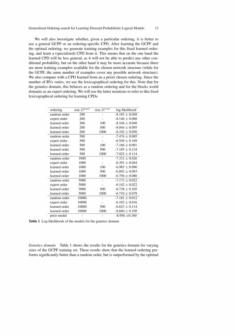
ordering size Dgcpf size Dregr log-likelihoodrandom order 200 - -8.185 ± 0.048expert order 200 - -8.146 ± 0.068learned order 200 100 -8.104 ± 0.048learned order 200 500 -8.044 ± 0.095learned order 200 1000 -8.102 ± 0.050random order 500 - -7.474 ± 0.085expert order 500 - -6.549 ± 0.169learned order 500 100 -7.166 ± 0.091learned order 500 500 -7.185 ± 0.124learned order 500 1000 -7.022 ± 0.114random order 1000 - -7.331 ± 0.026expert order 1000 - -6.391 ± 0.044learned order 1000 100 -6.985 ± 0.090learned order 1000 500 -6.892 ± 0.093learned order 1000 1000 -6.756 ± 0.086random order 5000 - -7.173 ± 0.022expert order 5000 - -6.142 ± 0.022learned order 5000 500 -6.738 ± 0.105learned order 5000 1000 -6.710 ± 0.078random order 10000 - -7.181 ± 0.012expert order 10000 - -6.103 ± 0.016learned order 10000 500 -6.623 ± 0.114learned order 10000 1000 -6.660 ± 0.109prior model - - -8.956 ±0.160
Table 1 Log-likelihoods of the models for the genetics domain
Genetics domain Table 1 shows the results for the genetics domain for varyingsizes of the GCPF training set. These results show that the learned ordering per-forms significantly better than a random order, but is outperformed by the optimal
14 Jan Ramon et al.
ordering. Also observe that for this domain a reasonably good ordering is learnedwith a small number of examples in Dregr.
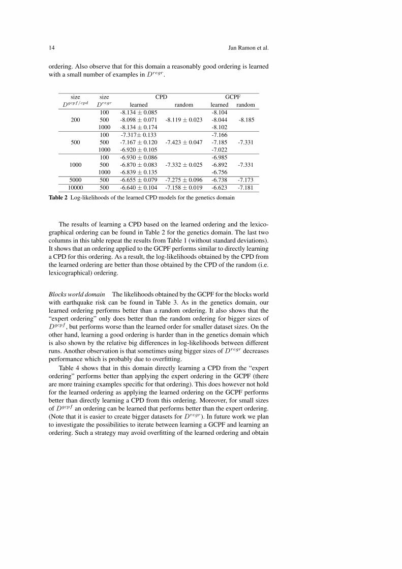
size size CPD GCPFDgcpf/cpd Dregr learned random learned random
200100 -8.134 ± 0.085
-8.119 ± 0.023-8.104
-8.185500 -8.098 ± 0.071 -8.0441000 -8.134 ± 0.174 -8.102
500100 -7.317± 0.133
-7.423 ± 0.047-7.166
-7.331500 -7.167 ± 0.120 -7.1851000 -6.920 ± 0.105 -7.022
1000100 -6.930 ± 0.086
-7.332 ± 0.025-6.985
-7.331500 -6.870 ± 0.083 -6.8921000 -6.839 ± 0.135 -6.756
5000 500 -6.655 ± 0.079 -7.275 ± 0.096 -6.738 -7.17310000 500 -6.640 ± 0.104 -7.158 ± 0.019 -6.623 -7.181
Table 2 Log-likelihoods of the learned CPD models for the genetics domain
The results of learning a CPD based on the learned ordering and the lexico-graphical ordering can be found in Table 2 for the genetics domain. The last twocolumns in this table repeat the results from Table 1 (without standard deviations).It shows that an ordering applied to the GCPF performs similar to directly learninga CPD for this ordering. As a result, the log-likelihoods obtained by the CPD fromthe learned ordering are better than those obtained by the CPD of the random (i.e.lexicographical) ordering.
Blocks world domain The likelihoods obtained by the GCPF for the blocks worldwith earthquake risk can be found in Table 3. As in the genetics domain, ourlearned ordering performs better than a random ordering. It also shows that the“expert ordering” only does better than the random ordering for bigger sizes ofDgcpf , but performs worse than the learned order for smaller dataset sizes. On theother hand, learning a good ordering is harder than in the genetics domain whichis also shown by the relative big differences in log-likelihoods between differentruns. Another observation is that sometimes using bigger sizes of Dregr decreasesperformance which is probably due to overfitting.
Table 4 shows that in this domain directly learning a CPD from the “expertordering” performs better than applying the expert ordering in the GCPF (thereare more training examples specific for that ordering). This does however not holdfor the learned ordering as applying the learned ordering on the GCPF performsbetter than directly learning a CPD from this ordering. Moreover, for small sizesof Dgcpf an ordering can be learned that performs better than the expert ordering.(Note that it is easier to create bigger datasets for Dregr). In future work we planto investigate the possibilities to iterate between learning a GCPF and learning anordering. Such a strategy may avoid overfitting of the learned ordering and obtain
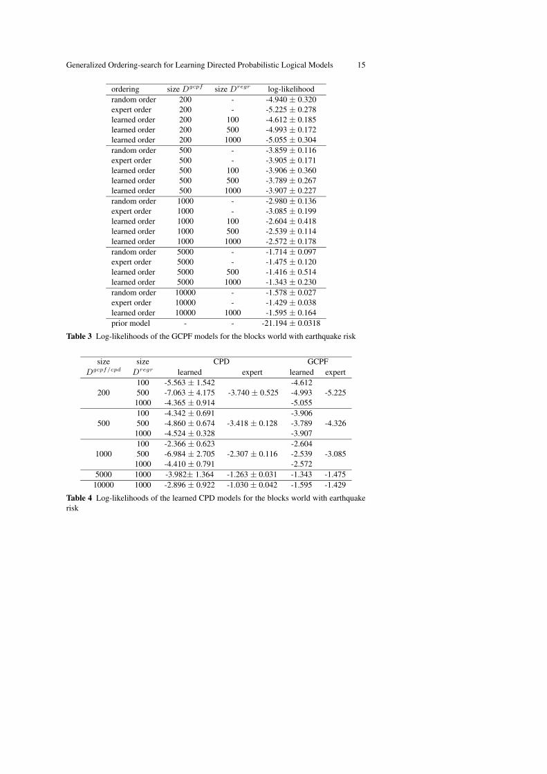
Generalized Ordering-search for Learning Directed Probabilistic Logical Models 15
ordering size Dgcpf size Dregr log-likelihoodrandom order 200 - -4.940 ± 0.320expert order 200 - -5.225 ± 0.278learned order 200 100 -4.612 ± 0.185learned order 200 500 -4.993 ± 0.172learned order 200 1000 -5.055 ± 0.304random order 500 - -3.859 ± 0.116expert order 500 - -3.905 ± 0.171learned order 500 100 -3.906 ± 0.360learned order 500 500 -3.789 ± 0.267learned order 500 1000 -3.907 ± 0.227random order 1000 - -2.980 ± 0.136expert order 1000 - -3.085 ± 0.199learned order 1000 100 -2.604 ± 0.418learned order 1000 500 -2.539 ± 0.114learned order 1000 1000 -2.572 ± 0.178random order 5000 - -1.714 ± 0.097expert order 5000 - -1.475 ± 0.120learned order 5000 500 -1.416 ± 0.514learned order 5000 1000 -1.343 ± 0.230random order 10000 - -1.578 ± 0.027expert order 10000 - -1.429 ± 0.038learned order 10000 1000 -1.595 ± 0.164prior model - - -21.194 ± 0.0318
Table 3 Log-likelihoods of the GCPF models for the blocks world with earthquake risk
size size CPD GCPFDgcpf/cpd Dregr learned expert learned expert
200100 -5.563 ± 1.542
-3.740 ± 0.525-4.612
-5.225500 -7.063 ± 4.175 -4.9931000 -4.365 ± 0.914 -5.055
500100 -4.342 ± 0.691
-3.418 ± 0.128-3.906
-4.326500 -4.860 ± 0.674 -3.7891000 -4.524 ± 0.328 -3.907
1000100 -2.366 ± 0.623
-2.307 ± 0.116-2.604
-3.085500 -6.984 ± 2.705 -2.5391000 -4.410 ± 0.791 -2.572
5000 1000 -3.982± 1.364 -1.263 ± 0.031 -1.343 -1.47510000 1000 -2.896 ± 0.922 -1.030 ± 0.042 -1.595 -1.429
Table 4 Log-likelihoods of the learned CPD models for the blocks world with earthquakerisk
16 Jan Ramon et al.
a more accurate GCPF in the subspace of cases where it will be used together withthe eventual ordering.
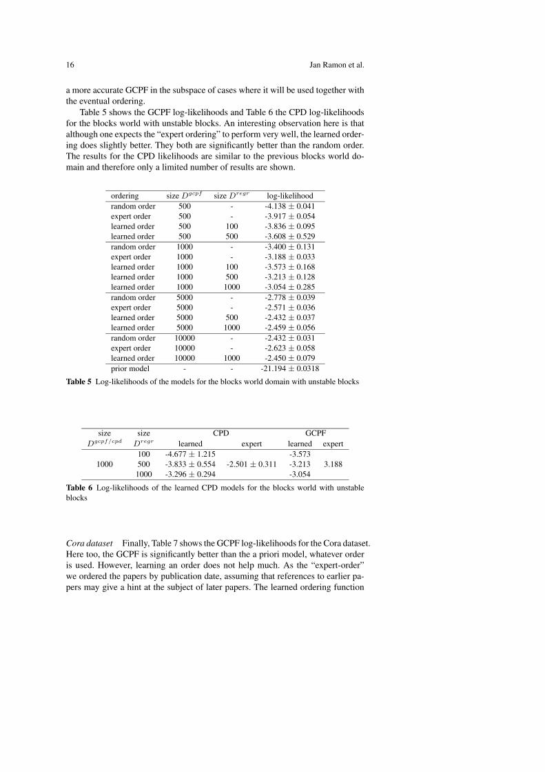
Table 5 shows the GCPF log-likelihoods and Table 6 the CPD log-likelihoodsfor the blocks world with unstable blocks. An interesting observation here is thatalthough one expects the “expert ordering” to perform very well, the learned order-ing does slightly better. They both are significantly better than the random order.The results for the CPD likelihoods are similar to the previous blocks world do-main and therefore only a limited number of results are shown.
ordering size Dgcpf size Dregr log-likelihoodrandom order 500 - -4.138 ± 0.041expert order 500 - -3.917 ± 0.054learned order 500 100 -3.836 ± 0.095learned order 500 500 -3.608 ± 0.529random order 1000 - -3.400 ± 0.131expert order 1000 - -3.188 ± 0.033learned order 1000 100 -3.573 ± 0.168learned order 1000 500 -3.213 ± 0.128learned order 1000 1000 -3.054 ± 0.285random order 5000 - -2.778 ± 0.039expert order 5000 - -2.571 ± 0.036learned order 5000 500 -2.432 ± 0.037learned order 5000 1000 -2.459 ± 0.056random order 10000 - -2.432 ± 0.031expert order 10000 - -2.623 ± 0.058learned order 10000 1000 -2.450 ± 0.079prior model - - -21.194 ± 0.0318
Table 5 Log-likelihoods of the models for the blocks world domain with unstable blocks
size size CPD GCPFDgcpf/cpd Dregr learned expert learned expert
1000100 -4.677 ± 1.215
-2.501 ± 0.311-3.573
3.188500 -3.833 ± 0.554 -3.2131000 -3.296 ± 0.294 -3.054
Table 6 Log-likelihoods of the learned CPD models for the blocks world with unstableblocks
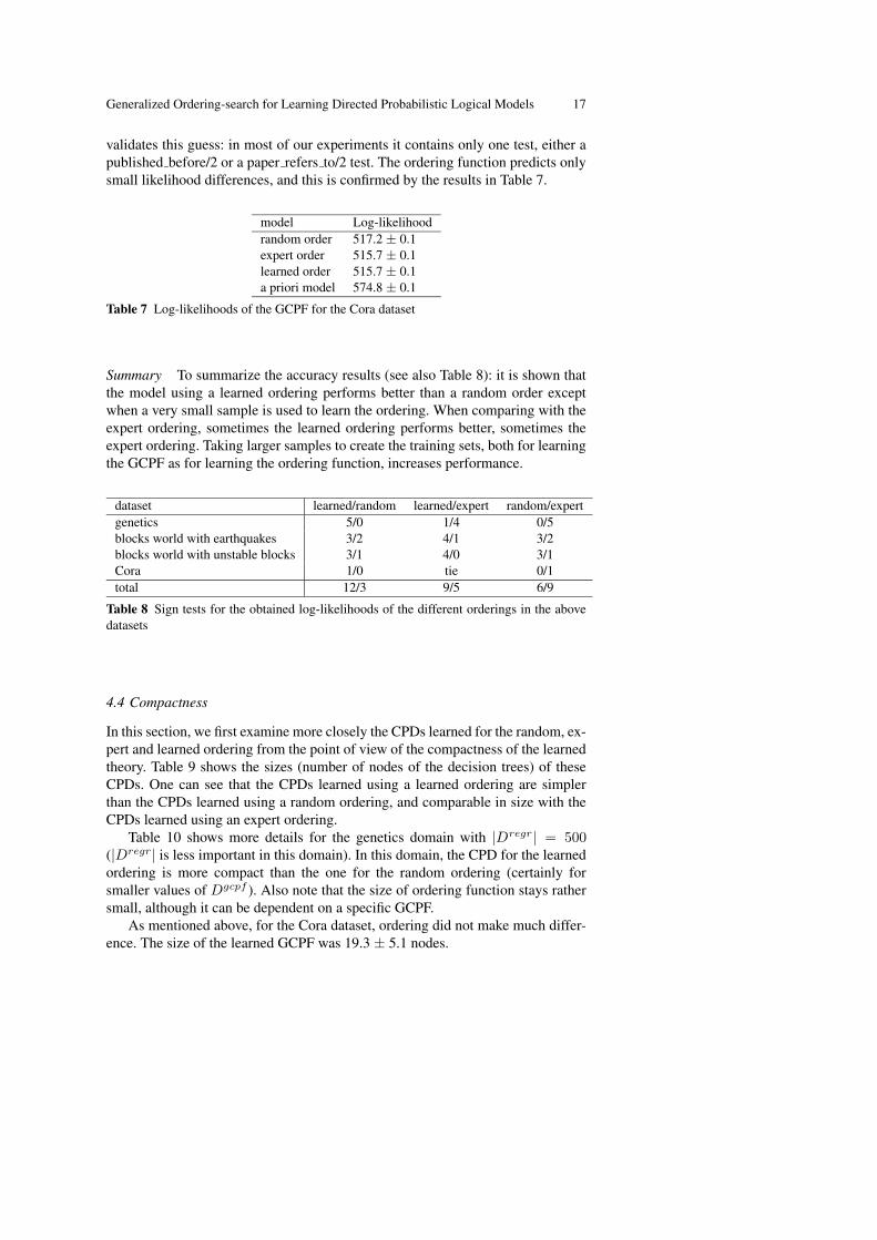
Cora dataset Finally, Table 7 shows the GCPF log-likelihoods for the Cora dataset.Here too, the GCPF is significantly better than the a priori model, whatever orderis used. However, learning an order does not help much. As the “expert-order”we ordered the papers by publication date, assuming that references to earlier pa-pers may give a hint at the subject of later papers. The learned ordering function
Generalized Ordering-search for Learning Directed Probabilistic Logical Models 17
validates this guess: in most of our experiments it contains only one test, either apublished before/2 or a paper refers to/2 test. The ordering function predicts onlysmall likelihood differences, and this is confirmed by the results in Table 7.
model Log-likelihoodrandom order 517.2 ± 0.1expert order 515.7 ± 0.1learned order 515.7 ± 0.1a priori model 574.8 ± 0.1
Table 7 Log-likelihoods of the GCPF for the Cora dataset
Summary To summarize the accuracy results (see also Table 8): it is shown thatthe model using a learned ordering performs better than a random order exceptwhen a very small sample is used to learn the ordering. When comparing with theexpert ordering, sometimes the learned ordering performs better, sometimes theexpert ordering. Taking larger samples to create the training sets, both for learningthe GCPF as for learning the ordering function, increases performance.
dataset learned/random learned/expert random/expertgenetics 5/0 1/4 0/5blocks world with earthquakes 3/2 4/1 3/2blocks world with unstable blocks 3/1 4/0 3/1Cora 1/0 tie 0/1total 12/3 9/5 6/9
Table 8 Sign tests for the obtained log-likelihoods of the different orderings in the abovedatasets
4.4 Compactness
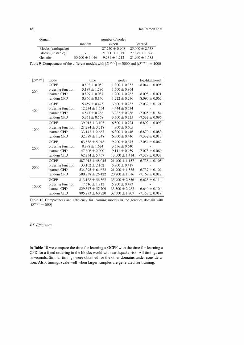
In this section, we first examine more closely the CPDs learned for the random, ex-pert and learned ordering from the point of view of the compactness of the learnedtheory. Table 9 shows the sizes (number of nodes of the decision trees) of theseCPDs. One can see that the CPDs learned using a learned ordering are simplerthan the CPDs learned using a random ordering, and comparable in size with theCPDs learned using an expert ordering.
Table 10 shows more details for the genetics domain with |Dregr| = 500(|Dregr| is less important in this domain). In this domain, the CPD for the learnedordering is more compact than the one for the random ordering (certainly forsmaller values of Dgcpf ). Also note that the size of ordering function stays rathersmall, although it can be dependent on a specific GCPF.
As mentioned above, for the Cora dataset, ordering did not make much differ-ence. The size of the learned GCPF was 19.3 ± 5.1 nodes.
18 Jan Ramon et al.
domain number of nodesrandom expert learned
Blocks (earthquake) - 27.250 ± 0.908 25.000 ± 2.538Blocks (unstable) - 21.000 ± 1.030 27.875 ± 1.696Genetics 30.200 ± 1.016 9.231 ± 1.712 21.900 ± 1.535
Table 9 Compactness of the different models with |Dgcpf | = 5000 and |Dregr| = 1000
|Dgcpf | mode time nodes log-likelihood
200
GCPF 0.802 ± 0.052 1.300 ± 0.353 -8.044 ± 0.095ordering function 5.189 ± 1.796 1.600 ± 0.864 -learned CPD 0.899 ± 0.087 1.200 ± 0.263 -8.098 ± 0.071random CPD 0.866 ± 0.140 1.222 ± 0.236 -8.090 ± 0.067
400
GCPF 5.459 ± 0.473 3.600 ± 0.233 -7.032 ± 0.121ordering function 12.734 ± 1.554 4.444 ± 0.534 -learned CPD 4.547 ± 0.288 3.222 ± 0.236 -7.025 ± 0.184random CPD 5.351 ± 0.568 3.700 ± 0.225 -7.532 ± 0.096
1000
GCPF 39.013 ± 3.103 6.500 ± 0.724 -6.892 ± 0.093ordering function 21.284 ± 3.718 4.800 ± 0.605 -learned CPD 33.142 ± 2.667 6.300 ± 0.446 -6.870 ± 0.083random CPD 32.389 ± 1.748 6.300 ± 0.446 -7.332 ± 0.017
2000
GCPF 63.838 ± 5.948 9.900 ± 0.675 -7.054 ± 0.062ordering function 8.898 ± 1.624 3.556 ± 0.640 -learned CPD 47.606 ± 2.000 9.111 ± 0.959 -7.073 ± 0.060random CPD 62.234 ± 5.457 13.000 ± 1.414 -7.329 ± 0.037
5000
GCPF 487.013 ± 48.045 21.400 ± 1.157 -6.738 ± 0.105ordering function 33.102 ± 2.162 5.700 ± 0.417 -learned CPD 534.395 ± 64.672 21.900 ± 1.535 -6.737 ± 0.109random CPD 500.938 ± 26.422 20.200 ± 1.016 -7.169 ± 0.017
10000
GCPF 813.168 ± 56.362 35.900 ± 2.856 -6.623 ± 0.114ordering function 17.516 ± 1.212 5.700 ± 0.473 -learned CPD 829.347 ± 57.709 33.300 ± 2.982 -6.640 ± 0.104random CPD 805.273 ± 60.820 32.300 ± 1.707 -7.158 ± 0.019
Table 10 Compactness and efficiency for learning models in the genetics domain with|Dregr = 500|
4.5 Efficiency
In Table 10 we compare the time for learning a GCPF with the time for learning aCPD for a fixed ordering in the blocks world with earthquake risk. All timings arein seconds. Similar timings were obtained for the other domains under considera-tion. Also, timings scale well when larger samples are generated for training.
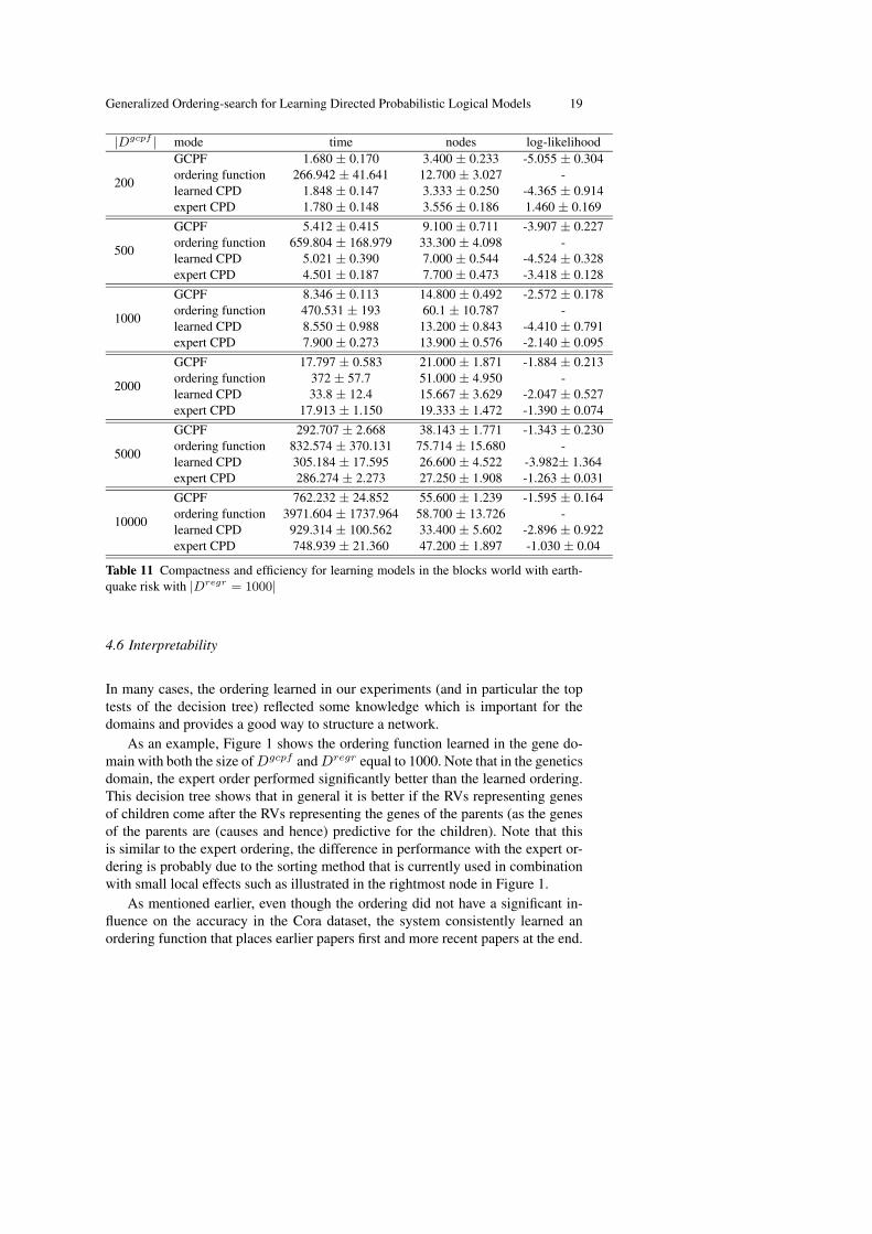
Generalized Ordering-search for Learning Directed Probabilistic Logical Models 19
|Dgcpf | mode time nodes log-likelihood
200
GCPF 1.680 ± 0.170 3.400 ± 0.233 -5.055 ± 0.304ordering function 266.942 ± 41.641 12.700 ± 3.027 -learned CPD 1.848 ± 0.147 3.333 ± 0.250 -4.365 ± 0.914expert CPD 1.780 ± 0.148 3.556 ± 0.186 1.460 ± 0.169
500
GCPF 5.412 ± 0.415 9.100 ± 0.711 -3.907 ± 0.227ordering function 659.804 ± 168.979 33.300 ± 4.098 -learned CPD 5.021 ± 0.390 7.000 ± 0.544 -4.524 ± 0.328expert CPD 4.501 ± 0.187 7.700 ± 0.473 -3.418 ± 0.128
1000
GCPF 8.346 ± 0.113 14.800 ± 0.492 -2.572 ± 0.178ordering function 470.531 ± 193 60.1 ± 10.787 -learned CPD 8.550 ± 0.988 13.200 ± 0.843 -4.410 ± 0.791expert CPD 7.900 ± 0.273 13.900 ± 0.576 -2.140 ± 0.095
2000
GCPF 17.797 ± 0.583 21.000 ± 1.871 -1.884 ± 0.213ordering function 372 ± 57.7 51.000 ± 4.950 -learned CPD 33.8 ± 12.4 15.667 ± 3.629 -2.047 ± 0.527expert CPD 17.913 ± 1.150 19.333 ± 1.472 -1.390 ± 0.074
5000
GCPF 292.707 ± 2.668 38.143 ± 1.771 -1.343 ± 0.230ordering function 832.574 ± 370.131 75.714 ± 15.680 -learned CPD 305.184 ± 17.595 26.600 ± 4.522 -3.982± 1.364expert CPD 286.274 ± 2.273 27.250 ± 1.908 -1.263 ± 0.031
10000
GCPF 762.232 ± 24.852 55.600 ± 1.239 -1.595 ± 0.164ordering function 3971.604 ± 1737.964 58.700 ± 13.726 -learned CPD 929.314 ± 100.562 33.400 ± 5.602 -2.896 ± 0.922expert CPD 748.939 ± 21.360 47.200 ± 1.897 -1.030 ± 0.04
Table 11 Compactness and efficiency for learning models in the blocks world with earth-quake risk with |Dregr = 1000|
4.6 Interpretability
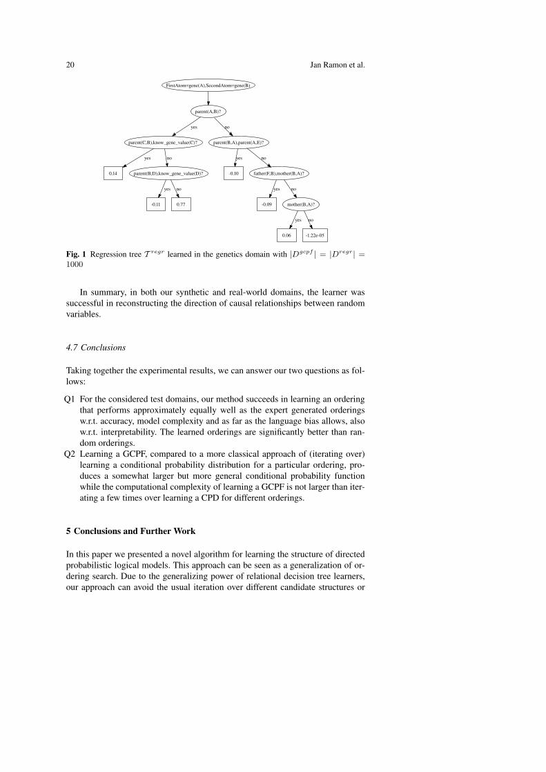
In many cases, the ordering learned in our experiments (and in particular the toptests of the decision tree) reflected some knowledge which is important for thedomains and provides a good way to structure a network.
As an example, Figure 1 shows the ordering function learned in the gene do-main with both the size of Dgcpf and Dregr equal to 1000. Note that in the geneticsdomain, the expert order performed significantly better than the learned ordering.This decision tree shows that in general it is better if the RVs representing genesof children come after the RVs representing the genes of the parents (as the genesof the parents are (causes and hence) predictive for the children). Note that thisis similar to the expert ordering, the difference in performance with the expert or-dering is probably due to the sorting method that is currently used in combinationwith small local effects such as illustrated in the rightmost node in Figure 1.
As mentioned earlier, even though the ordering did not have a significant in-fluence on the accuracy in the Cora dataset, the system consistently learned anordering function that places earlier papers first and more recent papers at the end.
20 Jan Ramon et al.
FirstAtom=gene(A),SecondAtom=gene(B)
parent(A,B)?
parent(C,B),know_gene_value(C)?
yes
parent(B,A),parent(A,E)?
no
0.14
yes
parent(B,D),know_gene_value(D)?
no
-0.11
yes
0.77
no
-0.10
yes
father(F,B),mother(B,A)?
no
-0.09
yes
mother(B,A)?
no
0.06
yes
-1.22e-05
no
Fig. 1 Regression tree T regr learned in the genetics domain with |Dgcpf | = |Dregr| =1000
In summary, in both our synthetic and real-world domains, the learner wassuccessful in reconstructing the direction of causal relationships between randomvariables.
4.7 Conclusions
Taking together the experimental results, we can answer our two questions as fol-lows:
Q1 For the considered test domains, our method succeeds in learning an orderingthat performs approximately equally well as the expert generated orderingsw.r.t. accuracy, model complexity and as far as the language bias allows, alsow.r.t. interpretability. The learned orderings are significantly better than ran-dom orderings.
Q2 Learning a GCPF, compared to a more classical approach of (iterating over)learning a conditional probability distribution for a particular ordering, pro-duces a somewhat larger but more general conditional probability functionwhile the computational complexity of learning a GCPF is not larger than iter-ating a few times over learning a CPD for different orderings.
5 Conclusions and Further Work
In this paper we presented a novel algorithm for learning the structure of directedprobabilistic logical models. This approach can be seen as a generalization of or-dering search. Due to the generalizing power of relational decision tree learners,our approach can avoid the usual iteration over different candidate structures or
Generalized Ordering-search for Learning Directed Probabilistic Logical Models 21
orderings by following a two-phase learning process. We have implemented ouralgorithm and presented promising empirical results.
There are several directions for further work. First, we would like to evaluateour algorithm on larger real-world datasets with multiple probabilistic predicatessince in the present paper we considered only datasets with one probabilistic pred-icate and we focussed on how to model recursive dependencies for this predicate.A second direction for further work is the development of a more general represen-tation of the model of the optimal ordering. Currently we use a regression tree thatspecifies for each two RVs which RV should be first in the ordering. This is a ratherlocal model. It is interesting to investigate whether an ordering can be specified ina more global way. This would allow us to avoid the use of bubblesort to deter-mine a concrete ordering and could be beneficial since in our current approachthe result of the bubblesort depends on the initial (lexicographical) ordering. Athird direction of future work is the investigation of more iterative methods whereafter learning a GCPF and an ordering, the ordering is used to generate trainingexamples that are more interesting than the original random ones.
Acknowledgements Jan Ramon and Hendrik Blockeel are post-doctoral fellows of theFund for Scientific Research of Flanders (FWO-Vlaanderen). Tom Croonenborghs andDaan Fierens are supported by the Institute for the Promotion of Innovation by Scienceand Technology in Flanders (IWT Vlaanderen).
References
Blockeel, H., & De Raedt, L. (1998). Top-down induction of first order logicaldecision trees. Artificial Intelligence, 101(1-2), 285-297.
Croonenborghs, T., Ramon, J., Blockeel, H., & Bruynooghe, M. (2007). On-line learning and exploiting relational models in reinforcement learning. InM. Veloso (Ed.), Proceedings of the 20th International Joint Conference onArtificial Intelligence (p. 726-731). Hyderabad, India: AAAI press.
De Raedt, L., & Kersting, K. (2004). Probabilistic inductive logic programming. InProceedings of the 15th International Conference on Algorithmic LearningTheory (Vol. 3244, p. 19-36). Lecture Notes in Computer Science, Springer.
Fierens, D., Blockeel, H., Bruynooghe, M., & Ramon, J. (2005). Logical Bayesiannetworks and their relation to other probabilistic logical models. In Proceed-ings of the 15th International Conference on Inductive Logic Programming(Vol. 3625, p. 121-135). Lecture Notes in Computer Science, Springer.
Fierens, D., Ramon, J., Blockeel, H., & Bruynooghe, M. (2005). A comparisonof approaches for learning first-order logical probability estimation trees.In 15th International Conference on Inductive Logic Programming, Late-breaking papers (p. 11-16). Technische Universitat Munchen. (TechnicalReport TUM-I0510, Technische Universitat Munchen).
Getoor, L., Friedman, N., Koller, D., & Pfeffer, A. (2001). Learning ProbabilisticRelational Models. In S. Dzeroski & N. Lavrac (Eds.), Relational DataMining (pp. 307–334). Springer-Verlag.
22 Jan Ramon et al.
Heckerman, D., Geiger, D., & Chickering, D. (1995). Learning Bayesian net-works: The combination of knowledge and statistical data. Machine Learn-ing, 20, 197-243.
Kersting, K., & De Raedt, L. (2001). Towards combining inductive logic pro-gramming and Bayesian networks. In C. Rouveirol & M. Sebag (Eds.),Proceedings of the 11th International Conference on Inductive Logic Pro-gramming (Vol. 2157, p. 118-131). Lecture Notes in Computer Science,Springer-Verlag.
McCallum, A., Nigam, K., Rennie, J., & Seymore, K. (1999). A machine learningapproach to building domain-specific search engines. In Proceedings of the16th International Joint Conference on Artificial Intelligence (pp. 662–667).Morgan Kaufmann.
Neapolitan, R. (2003). Learning Bayesian Networks. Upper Saddle River, NJ,USA: Prentice Hall.
Neville, J., & Jensen, D. (2004). Dependency networks for relational data. In Pro-ceedings of the 4th IEEE International Conference on Data Mining. IEEEComputer Society.
Neville, J., Jensen, D., Friedland, L., & Hay, M. (2003). Learning relationalprobability trees. In Proceedings of the 9th ACM SIGKDD InternationalConference on Knowledge Discovery and Data Mining. ACM.
Richardson, M., & Domingos, P. (2006). Markov logic networks. Machine Learn-ing, 62(1–2), 107–136.
Slaney, J., & Thiebaux, S. (2001). Blocks world revisited. Artificial Intelligence,125(1-2), 119–153.
Teyssier, M., & Koller, D. (2005). Ordering-based search: A simple and effec-tive algorithm for learning Bayesian networks. In Proceedings of the 21stConference on Uncertainty in AI (pp. 584–590). AUAI Press.