Embed Size (px)
Citation preview

Dynamic Interpolation Search
KURT MEHLHORN
Ma-Planck-I~zstitL{ tfiir Infomatik arzd UrtiL1ersitat des Saarlandes, Saarlandes, Germany
AND
ATHANASIOS TSAKALIDIS
Computer Technology Institate, Patras, Greece
Abstract. A new data structure called interpolation search tree (1ST) is presented which supportsinterpolation search and insertions and deletions. Amortized insertion and deletion cost isO(log n). The expected search time in a random file is O(log log n). This is not only true for the
uniform distribution but for a wide class of probability distributions.
Categories and Subject Descriptors: E. 1 [Data Structures]: trees; F.2 [Analysis of Algorithms andProblem Complexity]
General Terms: Algorithms
Additional Key Words and Phrases: Dynamization, interpolation search, search tree
1. Introduction
Interpolation search was first suggested by Peterson [11] as a method for
searching in sorted sequences stored in contiguous storage locations. The
expected running time of interpolation search on random files (generated
according to the uniform distribution) of size n is @(log log n). This was shown
by Yao and Yao [14], Pearl et al. [9], and Gonnet et al. [3]. A very intuitive
explanation of the behavior of interpolation search can be found in Pearl and
Reingold [10] (see also Mehlhorn [7]).
Dynamic interpolation search, that is, data structures that support insertions
and deletions as well as interpolation search, was discussed by Fredrickson [2],
and Itai et al. [5]. Fredrickson presents an implicit data structure that supports
insertions and deletions in time 0( n’), E > 0, and interpolation search with
expected time O(log log n). The structure of Itai et al. has expected insertion
A preliminary version of this paper was presented at ICALP ’85 and published in Proceedings of
ZCALP ’85. Lecture Notes in Computer Science, vol. 194. Springer-Verlag, New York, 1985, pp.22-23.
Authors addresses: K. Mehlhorn, M=-Planck-Institut fiir Informatik und Fachbereich Infor-matik, Universitat des Saarlandes, D-6600 Saarbriicken, Saarlandes. Germany; A. Tsakalidis,
Computer Technology Institute, P.O. Box 1122, 26110 Patras, Greece.
Permission to copy without fee all or part of this material is granted provided that the copies are
not made or distributed for direct commercial advantage, the ACM copyright notice and the title
of the publication and its date appear, and notice is given that copying is by permission of theAssociation for Computing Machinery. To copy otherwise, or to republish, requires a fee and/or
specific permission.01993 ACM 0004-5411/93/0700-0621 $01.50
Journal of the Awlclatlon for Computmg Machineq, Vol. 40, No. 3, July 1993, pp 621–634
622 K. MEHLHORN AND A. TSAKALIDIS
time O(log n) and amortized insertion time O((log n )Z). It is claimed to
support interpolation search, although no formal analysis of its expected
behavior is given. Both papers assume that files are generated according to the
uniform distribution. Other results on dynamic manipulation of sequential files
are given by Franklin [1], Melville and Gries [8], Hofri and Konheim [4], and
Willard [12].
Willard [13] extended interpolation search into another direction: nonuni-
form distributions. He showed that the log log n asymptotic retrieval time of
interpolation search does not remain in force for most nonuniform probability
distributions. However, he also introduced a variant of interpolation search and
showed that its expected running time is O(log log n) on static ~-random files
where w is any regular probability density. A density p, is regular if there are
constants bl, b2, b3, b4 such that V(X) = O for x < bl or x > b2 and K(X) >
b3 >0 and I w’(x)l s b4 for bl s x s b,. A file is ~-random if its elements are
drawn independently according to den;ity W. It is important to observe that
Willard’s algorithm does not have to know the density ~. Rather, its running
time is O(log log n) on N-random files provided that w is regular. Thus, his
algorithm is fairly robust.
In this paper, we combine and extend the research mentioned above. We
present a new data structure called interpolation search tree (1ST) that has the
following properties:
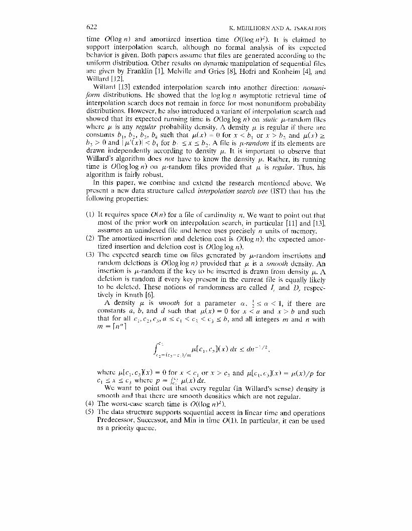
(1) It requires space O(n) for a file of cardinality 12. We want to point out thatmost of the prior work on interpolation search, in particular [11] and [13],
assumes an unindexed file and hence uses precisely n units of memory.
(2) The amortized insertion and deletion cost is O(log n); the expected amor-tized insertion and deletion cost is O(log log n).
(3) The expected search time on files generated by ~-random insertions andrandom deletions is O(log log n) provided that p is a smooth density. An
insertion is p-random if the key to be inserted is drawn from density p. A
deletion is random if every key present in the current file is equally likely
to be deleted. These notions of randomness are called 1, and D, respec-
tively in Knuth [6].
A density p is smooth for a parameter CY, ~ < a < 1, if there are
constants a, b, and d such that ~(x) = O for x < a and x > b and such
that for all cl, Cz, c~, a < c1 < C2 < C3 < b, and all integers m and n with
m = [rzal
1C2
dcI>cs](x)& < d~z-1\2,c2—(c3—cl )/m
where W[cl, c~](x) = O for x < c1 or x > c~ and p[cl, c~](x) = w(x)/p for
c1 s x s Cj where p = JC’,’K(x) &.
We want to point out that every regular (in Willard’s sense) density issmooth and that there are smooth densities which are not regular,
(4) The worst-case search time is O((log n)2).
(5) The data structure supports sequential access in linear time and operationsPredecessor, Successor, and Min in time O(l). In particular, it can be used
as a priority queue.
Qwamic Interpolation Search 623
This paper is structured as follows: In Section 2, interpolation search trees
are defined and the insertion and deletion algorithms are described and
analyzed. In Section 3, we then discuss the retrieval algorithm.
2. The Interpolation Search Tree
In this section, we introduce interpolation search trees (1ST) and discuss the
insertion and deletion algorithms.
An 1ST is a multiway tree where the degree of a node depends on the
cardinality of the set stored below it. More precisely, the degree of the root is
@(&). The root splits a file into @(v) subfiles. We do not postulate that the
subfiles have about equal sizes and in fact our insertion and deletion algo-
rithms will not enforce any such condition. In ideal ISTS, the subfiles have
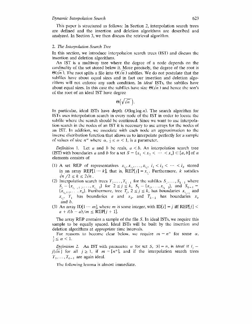
about equal sizes. In this case the subfiles have size (3(A) and hence the son’s
of the root of an ideal 1ST have degree
In particular, ideal ISTS have depth O(log log n). The search algorithm for
ISTS uses interpolation search in every node of the 1ST in order to locate the
subfile where the search should be continued. Since we want to use interpola-
tion search in the nodes of an 1ST it is necessary to use arrays for the nodes of
an 1ST. In addition, we associate with each node an approximation to the
inverse distribution function that allows us to interpolate perfectly for a sample
of values of size n” where a , ~ < a < 1, is a parameter.
Definition 1. Let a and b be reals, a < b. An interpolation search tree
(1ST) with boundaries a and b for a set S = {xl < Xz < “.” < x.} c [a, b] of nelements consists of
(1) A set REP of representatives ~i,, xi,,..., xi,, il < iz < “”” < i~ stored
in an array REP[l “”” k], that is, REP[j] = x,,. Furthermore, k satisfies
&/’2 s k < 2&.
(2) Interpolation search trees Tl,..., T~+ ~ for the subfiles S1,..., Sk+ ~ wheresJ={x,J_, +l,..., xi_l} for 2<j <k, S1 ={xl, . . ..xl. _l}, and S~+l =
{X1,+ l>...> x,,}. Furthermore, tree TJ, 2 s j s k, has boundaries x,, _, and
x T1 has boundaries a and xl, and T~~ ~ has boundaries x~
;;d b.
(3) An array ID[l . . . m], where m is some integer, with ID[i] = j iff REP[j] <
a + i(b – a)/m < REP[j + 1].
The array REP contains a sample of the file S. In ideal ISTS, we require this
sample to be equally spaced. Ideal ISTS will be built by the insertion and
deletion algorithms at appropriate time intervals.
For reasons to become clear below, we require m = n” for some a,
;<a <l.
Definition 2. An 1ST with parameter a for set S, IS 1 = n, is ideal if i, =
jlfil for all j > 1, if m = rn” 1, and if the interpolation search trees
Tl,. . . . T~+ ~ are again ideal.
The following lemma is almost immediate.
624 K. MEHLHORN AND A. TSAKALIDIS
LEMMA 1. Let ~ < a < 1.Then an ideal 1ST for an ordered set S, IS I = n, can
be built in time O(n) and requires space O(n). It has depth O(log logn).
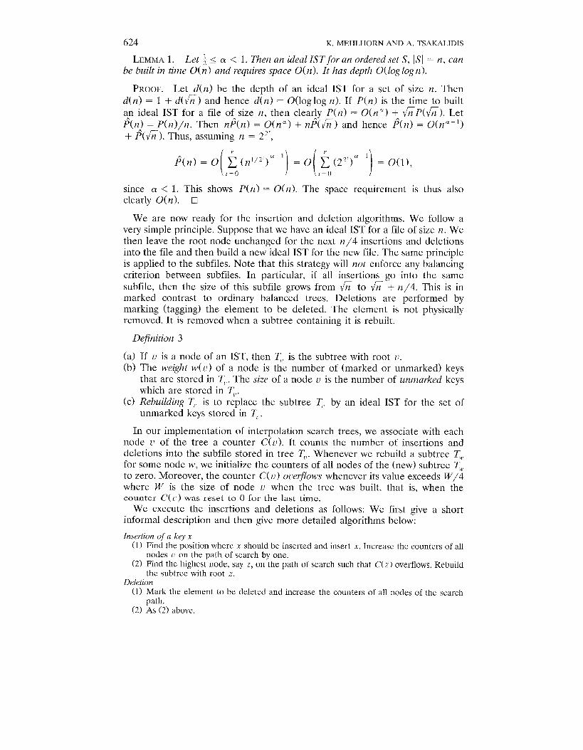
PROOF. Let d(n) be the depth of an ideal 1ST for a set of size n. Then
d(n) = 1 + d(h) and hence d(n) = O(log log n). If P(n) is the time to built
+n ideal 1ST for a file o: size n, then clearly P(n) = O(n” ) +A fiP(&). Let
P(~zj = P(n)/n. Then nP(n) = O(n”) + nP(fi) and hence P(n) = O(n”-l)
+ I’(h). Thus, assuming n = 22’,
[P(n) = O ~ (nl/Q1)”-l
~=(1 ) ‘0(A(22[)a-’1 =0(1)7
since a < 1. This shows P(?z) = O(n). The space requirement is thus also
clearly O(n). El
We are now ready for the insertion and deletion algorithms. We follow a
very simple principle. Suppose that we have an ideal 1ST for a file of size n. We
then leave the root node unchanged for the next n/4 insertions and deletions
into the file and then build a new ideal 1ST for the new file. The same principle
is applied to the subfiles. Note that this strategy will not enforce any balancing
criterion between subfiles. In particular, if all insertions go into the same
subfile, then the size of this subfile grows from fi to ~ + n/4. This is in
marked contrast to ordinary balanced trees. Deletions are performed by
marking (tagging) the element to be deleted. The element is not physically
removed. It is removed when a subtree containing it is rebuilt.
Definition 3
(a)
(b)
(c)
If u is a node of an 1ST, then T, is the subtree with root LI.
The weight w(u) of a node is the number of (marked or unmarked) keys
that are stored in ~,. The size of a node LI is the number of unmarked keys
which are stored in T,,.
Rebuilding T,, is to replace the subtree T,, by an ideal 1ST for the set of. .unmarked keys stored” in T,,.
In our implementation of interpolation search trees, we associate with each
node LI of the tree a counter C( ~~). It counts the number of insertions and
deletions into the subfile stored in tree TU. Whenever we rebuild a subtree Tw
for some node w, we initialize the counters of all nodes of the (new) subtree Tw
to zero. Moreover, the counter C(u) oL)erj-Zows whenever its value exceeds W/4
where W is the size of node v when the tree was built, that is, when thecounter C(L) was reset to O for the last time.
We execute the insertions and deletions as follows: We first give a short
informal description and then give more detailed algorithms below:
Insertion of a key x
(1) Find the position where x should be inserted and insert x. Increase the counters of allnodes 1) on the path of search by one.
(2) Find the highest node, say z, on the path of search such that C(z) overflows. Rebuildthe subtree with root z.
Deletion
(1) ~:~k the element to be deleted and increase the counters of all nodes of the search
(2) As (2) above.
h~lamic Interpolation Search 625
The intuition behind these algorithms is as follows:
(1) Good worst-case behavior for searches can be achieved if the weights along any path
from the root to a leaf are geometrically decreasing, because this will guarantee
logarithmic depth of the tree. The counters do exactly that: cf. Lemma 2 below. Good
worst-case behavior for insertions and deletions (at least in an amortized sense) can beachieved if nodes of size W remain unchanged for a time which is proportional to W.
This is also achieved by the counters. Note that a tree T,, of (initial) size W is onlyrebuilt after W\4 insertions or deletions into that subtree.
(2) Good average-case behavior for searches can be achieved if interpolation search (or avariant of it) can be used to search the arrays of representatives. In order for that towork, we need to know that the array of representatives stored in a node L? is a “fair”
sample of the file stored in subtree T,. We achieve this goal by not enforcing any
criterion that relates the size of the files stored in the direct sons of a node L}. Note that
in ordinary balanced trees an “overflow” at a node u changes not only node LI but alsoL]‘S father. In particular, in ordinary balanced trees an “overflow” at node t changes the
set of representatives stored in u‘s father. We found it impossible to do a satisfacto~
expected case analysis of any such scheme and therefore have chosen update algorithms
that do not enforce any balancing condition between brother nodes. This will imply inparticular, that the files that are stored in brother nodes can be treated as independentfiles.
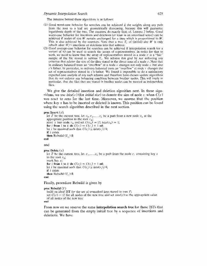
We give the detailed insertion and deletion algorithm next. In these algo-
rithms, we use isize( L) ) (for initial size) LO denote the size of node LI when C( L’)
was reset to zero for the last time. Moreover, we assume that the position
where key x has to be inserted or deleted is known. This position can be found
using the search algorithm described in the next section.
proc Insert (x);let T be the current tree. let Lo, L ~,..., Vk be a path from a new node Lo at the
appropriate position to the root LIk;
store .x into node LJOand set C( UO) = 0; isize( L’o) := 1;
for i from 1 to k do C(L),) := C(LIt) + 1 od;
let i be maximal such that C(L),) > isize(ul )/4;
if i existsthen Rebuild (T,,, ) fi
end
and
proc Delete (x)
let T be the current tree, let L’,,..., LIk be a path from the node z, containing key .t
to the root Uk;
mark key x;for i from 1 to k do C( LI,) := C( u,) + 1 od;
let i be maximal such that C(L),) > isize(ul)/4;
if z exists
then Rebuild (T,,t ) fi
end
Finally, procedure Rebuild is given by
proc Rebuild (T)build an ideal 1ST for the set of unmarked keys stored in tree T;
set C([) ) := @ for all nodes of the new tree and set isize( L’ ) to the appropriate valueof all nodes of the new tree
end
From now on we reserve the same interpolation search tree for those ISTS that
can be generated from the empty initial tree by a sequence of insertions and
deletions. We have
626 K, MEHLHORN AND A. TSAKALIDIS
LEMMA 2. The worst-case depth of an 1ST for a file of n keys is 0( log n). It
requires 0(n) storage space.
PROOF. We prove the bound on the depth first. Consider an arbitra~ node
ZI of an 1ST and let w = father( LI) be its father node. Then, at
most C(w) s isize(w)/4 insertions and deletions occurred in the subfile
represented by node L).
Hence, size(u) s ~- + isize(w)/4 < isize( w)/2 since the subfile rep-
resented by node LI started out with JiiiiiXT keys when TW was rebuilt for
the last time and has gained at most isize( w)/4 additional keys since then. We
conclude that the depth of an 1ST is O(log isize(root)). Since size(root) z
isize( root) – C(root) s isize(root)/2 and n = size(root ) we conclude that the
depth is O(log n).
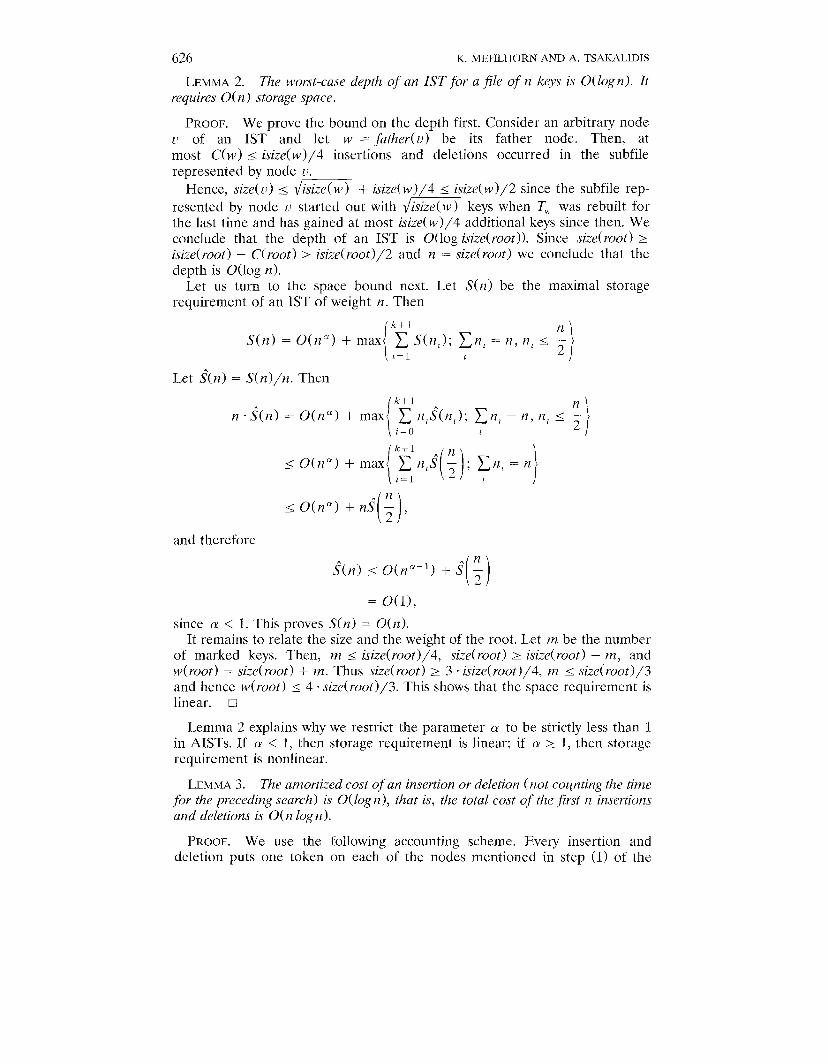
Let us turn to the space bound next. Let S(n) be the maximal storage
requirement of an 1ST of weight n. Then
Let j(n) = S(n)/n. Then
()*n
< O(na) +rzs j ,
and therefore
= 0(1),
since a < 1. This proves S(n) = 0(/z).
It remains to relate the size and the weight of the root. Let m be the number
of marked keys. Then, m s isize( root )/4, size( root) z isize(root ) – m, and
w(root ) = size( root) + m. Thus size( root) z 3. isize( root )/4, m < size(root)/3
and hence w(root) < 4. size(root)/3. This shows that the space requirement is
linear. ❑
Lemma 2 explains why we restrict the parameter a to be strictly less than 1
in AISTS. If a < 1, then storage requirement is linear: if a > 1, then storage
requirement is nonlinear.
LEMMA 3. The amortized cost of an insertion or deletion (not col~nting the time
for the preceding search) is O(log n), that is, the total cost of the first n insertions
and deletions is 0( n log n).
PROOF. We use the following accounting scheme. Every insertion and
deletion puts one token on each of the nodes mentioned in step (1) of the

Dynamic Interpolation Search 627
insertion or deletion algorithm. Then every node u of an 1ST holds C( ~’)
tokens and an insertion/deletion puts down O(log n) tokens by lemma z.A token represents the ability to pay for O(1) computing time. Suppose
now that we have to rebuild T,, for a cost of O(w( v)). Since W(u) s 5/4. isize( u )
and C(u) > i,size( u)/4 when TV is rebuilt we conclude that the tokens on nodeu suffice to pay for rebuilding tree ~,. ❑
3. Searching in Interpolation Search Trees
In this section, we discuss how to search in interpolation search trees in
expected time O(log log n).
The expected case running time is defined with respect to random files and
trees that we define next. We also derive some properties of random trees that
will be useful for the analysis. Let p be a probability density function on the
real line. We later put various restrictions on p. A random file of size n is
generated by drawing independently n reals according to density p. A random
1ST of size n is generated as follows:
(1) Take a random file F of size n’ for some n’ and build an ideal 1ST
for it.
(2) Perform a sequence Opl,..., Op,,, of p-random insertions and randomdeletions on this tree. Clearly, if there are i insertions and d deletions in
the sequence then m = i + d and n = n‘ + i – d. An insertion is pran-
dom if it inserts a random real drawn according to density p into the tree.
A deletion is random if it deletes a random element from the file, that is,
all elements in the file are equally likely to be chosen for the deletion.
These notions of randomness are called 1, and D,, respectively, in Knuth
[6].
The following two properties of random ISTS are very helpful: Subtrees of
random trees are again random and the size of subtree stays rootic with high
probability.
LEMMA 4. Let “p be a density function with jinite support [a, b], let T be a
p-random IST with boundaries a and b and let T‘ be a subtree of T. Then there
are reals c, d such that T‘ is a ~[c, d]-random IST.
PROOF. The tree T was constructed by starting with the ideal 1ST TO for a
random file FO and then applying a random sequence Opl, ..., OPH, of inser-
tions and deletions to it. Let F, be the file obtained after executing Opl, ..., Opt.
Then, F, is clearly a random file, since insertions insert elements drawn
according to p and deletions delete all elements in the current file with equal
probability.
Let m‘ s m be such that tree T‘ was built after executing Op., and was not
rebuilt since then. We have m‘ = O if T‘ exists in TO and was never rebuilt. Let
L’ be the root of T‘ and let w be the father of L’. Then, some ancestor of L’
overflowed when operation Op.,, was executed. Let c and d be the boundaries
of T‘. After executing Op~, tree T‘ is an ideal 1ST for file f,m,[c, d] ‘= {x G F,n ~;
c < x < d}. This file is a random file with respect to distribution v[c, d]. AlsoT‘ as it exists after processing Op,. can be obtained from T‘ as it was created
after processing Op.,, by applying the operations in Op~ ~+ 1, ..., OPn, that refer
to items between c and d. This is a sequence of w[c, d]-random insertions and
random deletions.
628 K. MEHLHORN AND A. TSAKALIDIS
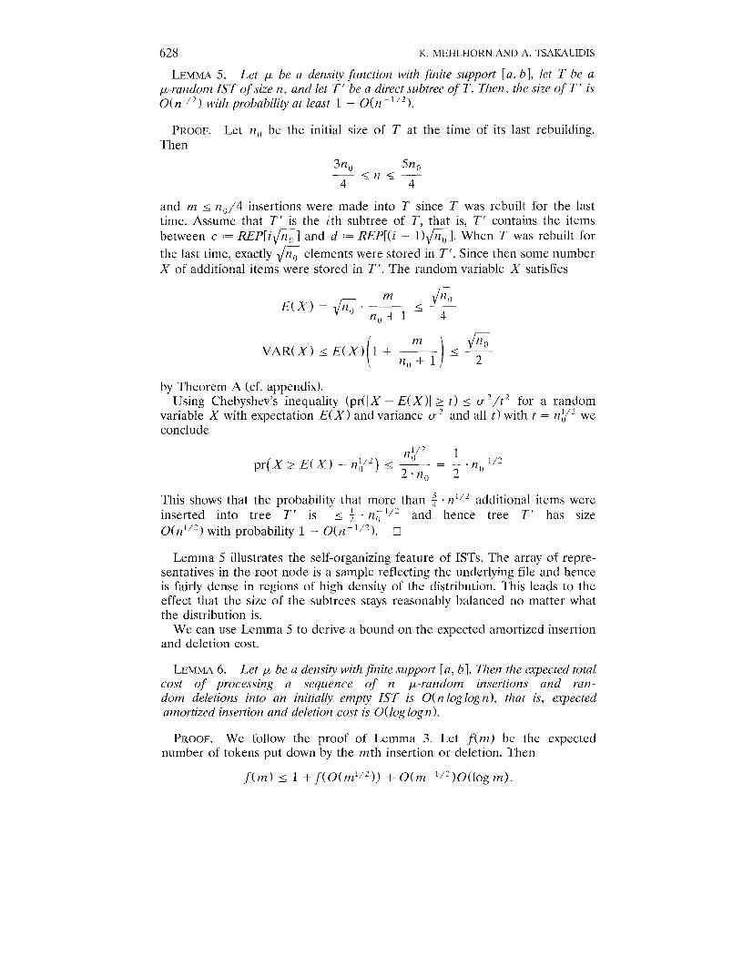
LEMMA 5. Let p be a densi~ fimction with finite sLlppoti [a, b], let T be a
p-random 1ST of size n, and let T‘ be a direct subtree of T. Then, the size of T‘ is
O(nl/~ ) with probability at least 1 – O(n -1 lz).
PROOF. Let no be the initial size of T at the time of its last rebuilding.
Then
%10 5n0—<n<-
4 4
and m s n “/4 insertions were made into T since T was rebuilt for the last
time. Assume that T‘ is the ith subtree of T, that is, T‘ contains the items
between c Z= REP[i&] and d := REP[(i + 1)~]. When T was rebuilt for
the last time, exactly fi elements were stored in T‘. Since then some number
X of additional items were stored in T’. The random variable X satisfies
.
by Theorem A (cf. appendix).
Using Chebyshev’s inequality (pr( IX – E(X) I z t) s o ‘/t 2 for a random
variable X with expectation E(X) and variance o z and all t)with t = n ~’z we
conclude
1/2no 1
pr(X > E(X) + n~lz~ s — = –1/2— . no
2 “ ?1,, 2
This shows that the probability that more than ~ ./Z l/z additional items were
inserted into tree T’ is < : .rz;lj~ and hence tree T‘ has size
O(nl/~) with probability 1 – O(?Z %. ❑
Lemma 5 illustrates the self-organizing feature of ISTS. The array of repre-
sentatives in the root node is a sample reflecting the underlying file and hence
is fairly dense in regions of high density of the distribution. This leads to the
effect that the size of the subtrees stays reasonably balanced no matter what
the distribution is.
We can use Lemma 5 to derive a bound on the expected amortized insertionand deletion cost.
LEMMA 6. Let v be a derlsip with jikite szlppoti [a, b]. Then the expected total
cost of processing a sequence of n p-rarzdorn insertiotzs and ran-
dom deletions into an initially empty 1ST is 0( n log log n), that is, expected
amortized insertion and deletion cost is O(log log n ).
PROOF. We follow the proof of Lemma 3. Let f(m) be the expected
number of tokens put down by the rnth insertion or deletion. Then
f(m) <1 +f(O(rnl/’)) + O(m-l/’)O(logrn).

Dynamic Interpolation Search 629
This can be seen as follows: If the insertion or deletion goes into a subtree of
size O(rn l\z), then we put down 1 + f(O(ml/2)) tokens. If it does not, then we
put down at most O(log m) tokens by Lemma 2. The probability of
the latter event is O(WZ - ‘/2) by Lemma 5. Thus, ~(nz) = O(log log m). •l
Searching ISTS is quite simple. Suppose that we have to search for y = R.
We can use the approximation ID to the inverse distribution function to obtain
a very good estimate for the position of y in the array of representatives. From
this initial guess, we can then determine the actual position of y by a simple
linear search. The details are as follows:
Let T be an 1ST with boundaries a and b. Let REP[l “o. k] and ID[l”. o ml
be the array of representatives and approximation to the inverse distribution,
respectively, associated with the root.
(1) j := ID[l((y - a)/(b - a))nzll
(2) while y > REP[j + 1] and j < k
(3) doj:=j+lod
(4) search the jth subtree using the same algorithm recursively
The correctness of this algorithm can be seen as follows:
Let i := [(y – a)m/(b – a)] = (y – a)m/(b – a) – e for some O < e <1.
Then
i(b – a)REP[j] < a + m s REP[j + 1].
This proves y > REP[ j ] and hence establishes correctness. The worst-case
search time WT(n) in an 1ST of size n is also easily derived. Clearly, at most
~(fi)-time units are spent in the root array. ~SO the subfile to be searched
has size at most n/2 and hence
()W’T(n) < O(&) + WT ~ ,
which solves for WT(n ) = O(h). The worst-case search time is easily im-
proved to O((log ~z)2) by using exponential and binary search instead of linearsearch. More precisely, compare y with REP[j], REP[j + 20],
REP[j + 21], REP[j + 2Z],..., until an 1 is found with REP[ j + 21-1] <
y < REP[j + 21]. Then, use binary search to finish the search. With this
modification, worst-case search time in the array is O(log n) and hence total
worst-case search time is O((log tZ)2).
Finally, observe that the number of search steps used by exponential + binary
search is O (number of steps taken by linear search) and hence the expected
case analysis done below also applies to exponential + binary search. Let us
turn to expected search time next.
LEMMA 7. Let p be a smooth densi~ for parameter a, ~ < a < 1, and let T
be a p-random IST with parameter a. Then, the expected se~rch time in the root
array is O(l).
630
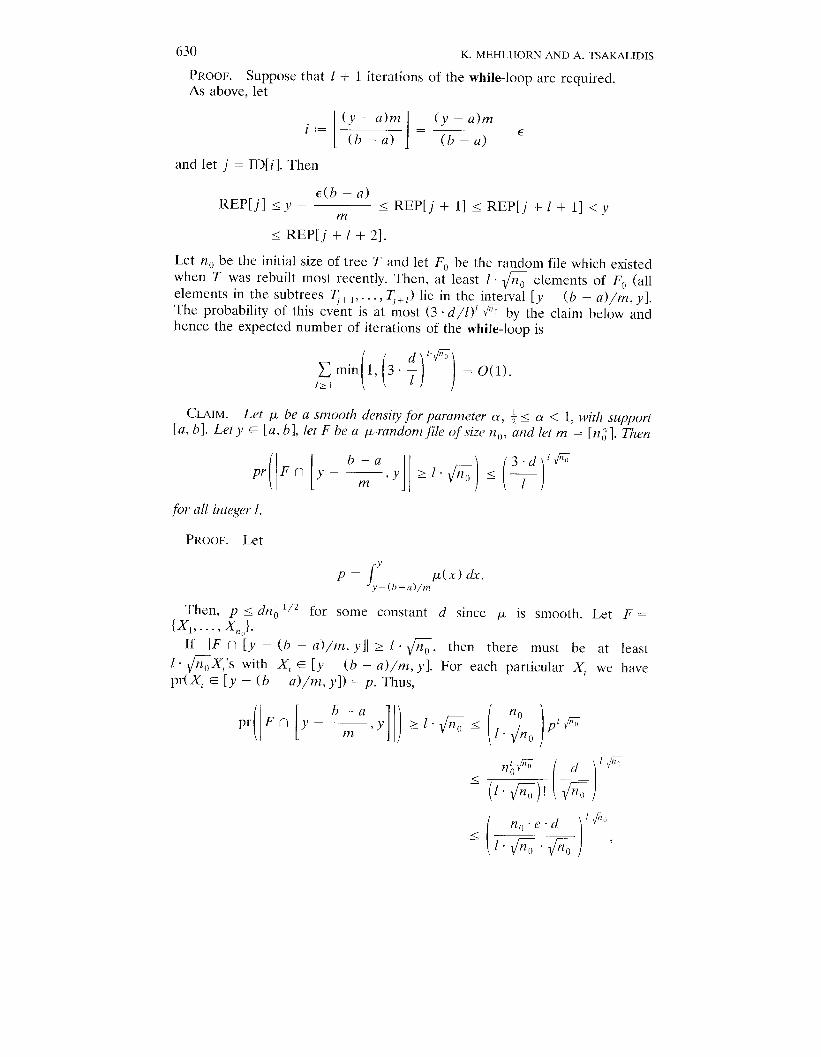
PROOF. Suppose
As above, let
K. MEHLHORN AND A. TSAKALIDIS
that 1 + 1 iterations of the while-loop are required.
H(y–a)m (y – a)mi :=
(b–a) = (b–a) “
and let j = ID[i]. Then
REP[j] <y –.5(b – a)
<REP[j+ l]< REP[j+l+l] <vm
< REP[j +1 + 2].
Let no be the initial size of tree T and let FO be the random file which existed
when T was rebuilt most recently. Then, at least 1. fi elements of FO (all
elements in the subtrees ~+,, . . ., T+{) lie in the interval [y – (b – a)/m, y].
The probability of this event is at most (3 “ d/1)~ @ by the claim below and
hence the expected number of iterations of the while-loop is
~min(1(3”:1’”&l=O(’)121
CLAIM. Let p be a smooth density for parameter CY,~ < a < 1, with support
[a, b]. Let y ~ [a, b], let F be a p-randonzfile of size n,), ‘&d let m = [n;]. Then
for all integer 1.
PROOF. Let
1p= y
/L(x)&.y–(b–a)/m
– 1’2 for some constant d since p is smooth.Then, p s dnO
{x,,.. ., X,,,l}.
lf [F n [y – (b – a)/m, y]l z 1. ~, then there must be
1- fiX,’s with X, E [y – (b – a)/m, y]. For each particular Xi
pr(X, = [y – (b – a)/m, y]) = p. Thus,
Let F =
at least
we have
\’@
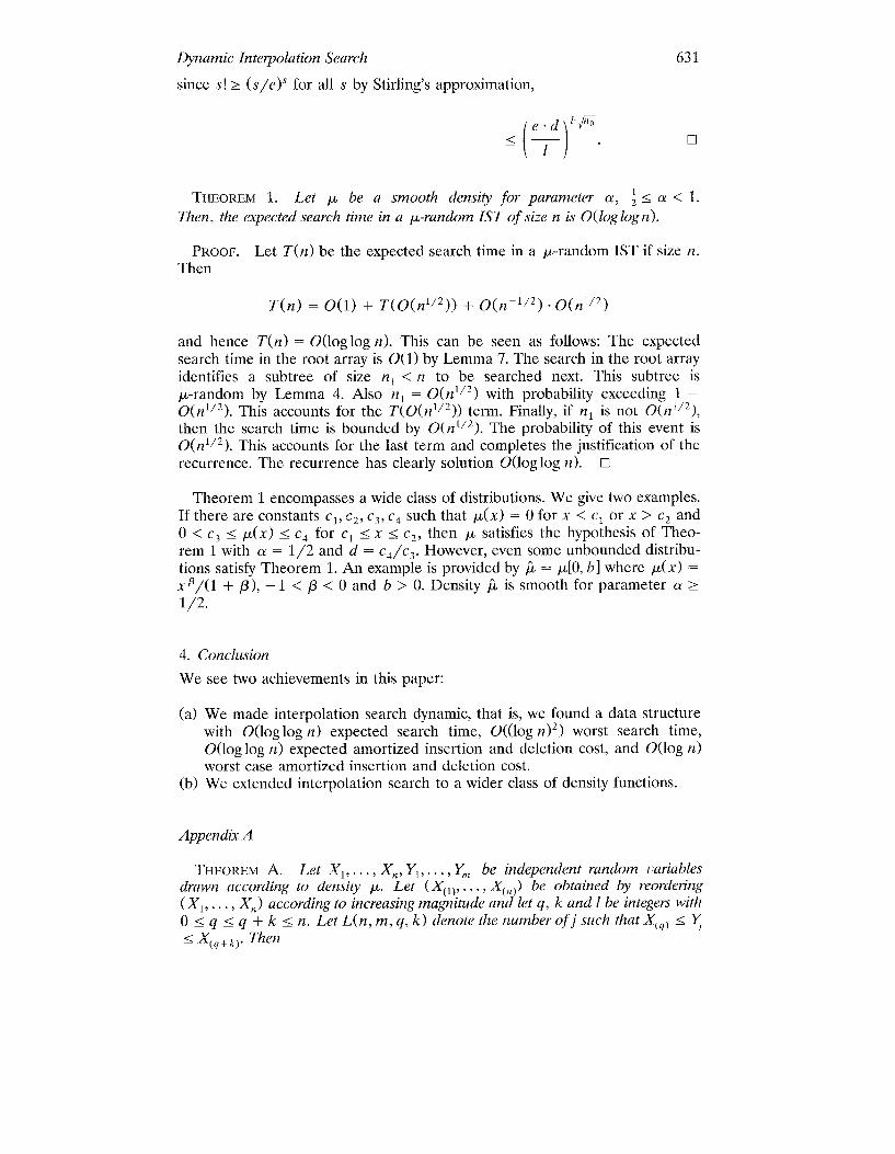
631Dynamic Interpolation Search
since s! > (s/e)s for all s by Stirling’s approximation,
e.d “K
()<—
1“❑
THEOREM 1. Let p be a smooth density for parameter a, ~ < a < 1.
Then, the expected search time in a p-random IST of size n is O(log log n).
PROOF. Let T(n) be the expected search time in a ~-random 1ST if size n.
Then
T(n) = O(1) + T(O(nl/2)) + O(n-1f2) “ O(nl/2)
and hence T(n) = O(log log n). This can be seen as follows: The expected
search time in the root array is O(1) by Lemma 7. The search in the root array
identifies a subtree of size n ~ < n to be searched next. This subtree is
~-random by Lemma 4. Also n ~ = O(n’/z ) with probability exceeding 1 –
O(nl/z). This accounts for the T(O(nllz)) term. Finally, if nl is not O(n’j2),
then the search time is bounded by 0( n’j2). The probability of this event is
O(nljz). This accounts for the last term and completes the justification of the
recurrence. The recurrence has clearly solution O(log log n). ❑
Theorem 1 encompasses a wide class of distributions. We give two examples.
If there are constants c1, C2, c~, Ci such that p(x) = O for x < c1 or x > C2 and
O<c~Sp(x) <cJforcl <x< Cz, then ~ satisfies the hypothesis of Theo-
rem 1 with a = 1/2 and d = cJ/c~. However, even some unbounded distribu-
tions satisfy Theorem 1. An example is provided by jl = KIO, b] where p(x) =
x ‘/(1 + ~), – 1 < ~ < 0 and b > 0. Density & is smooth for parameter a >
1/2.
4. Conclusion
We see two achievements in this paper:
(a) We made interpolation search dynamic, that is, we found a data structurewith O(log log n) expected search time, O((log n)2) worst search time,O(log log n) expected amortized insertion and deletion cost, and O(log n)
worst case amortized insertion and deletion cost.
(b) We extended interpolation search to a wider class of density functions.
Appendix A
THEOREM A. Let X1,. ... ,Y1,l,..., Y., be independent random variablesdrawn according to densip 1A. Let ( X( I,,..., X(,,)) be obtained by reordering
(x,, . . . . X,,) according to increasing magnitude and let q, k and 1 be integers with
O s q < q + k < n. Let L(n, m, q, k) denote the number of j such that Xt~) < ~s X(~+~l. Then

632
(a)
K. MEHLHORN AND A. TSAKALIDIS
Pr(L(n, m,q, k) = 1) =(’+f-’l(’’::~: k),),
(1
m + nm
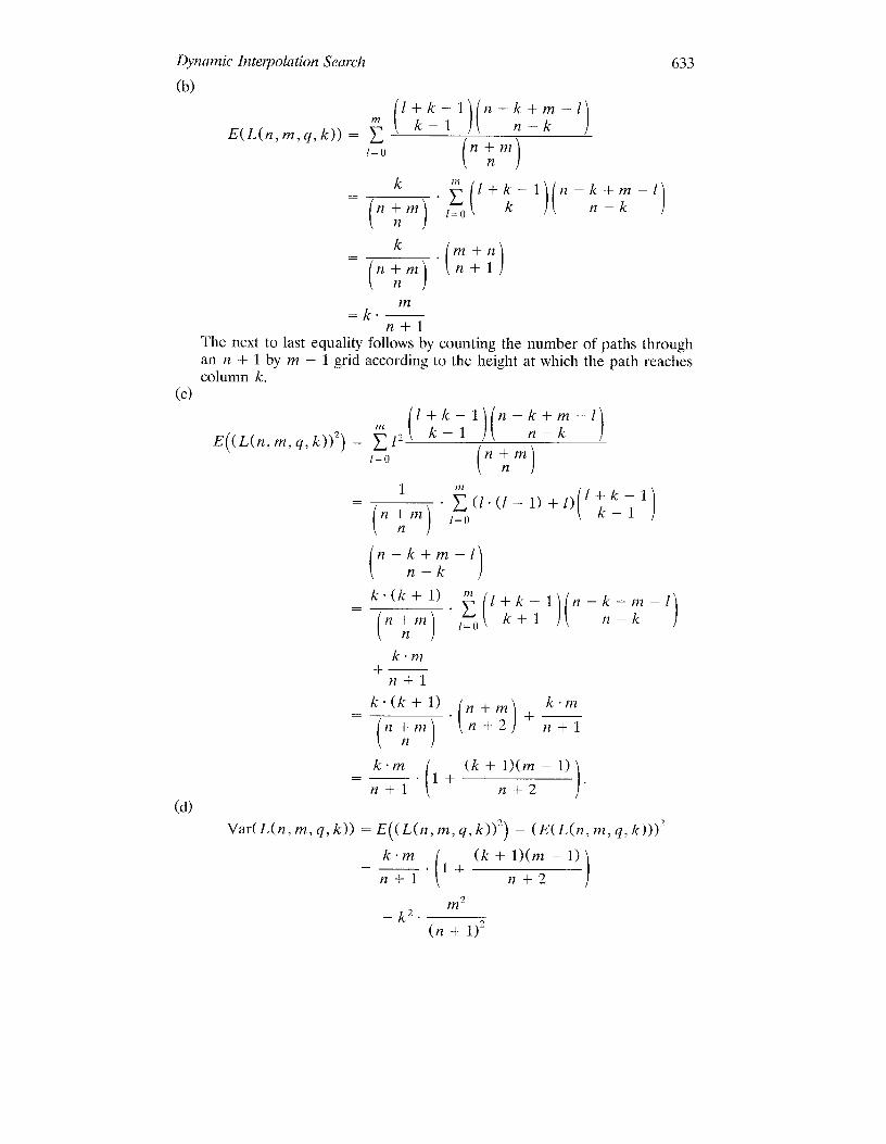
(b)
m
E(I,(n, m,q, k)) =k. —n+l’
(c)
(d)
I\L’ 11+1 )’
Viw(l, (n, m,q,k)) <k . nl
[
m—“l+—n+l )n+l’
PROOF
xl,..., xn, Y1,.. ., Yv, be reordering
()fixed Z1 . . . .. Z~+~. there are “j,’n
that yield this particular Z-sea uence.
(a) Let 21,...,2. +~ be obtained from
according to magnitude. Clearly, for
partitions {{X1,. . . . X.}, {Yl,..., Y~l})
How many of these partitions satisfy that_ there ar~ exactly lY’s b~tween
X[,,~ and X ~~+ ~)? Let us call this number C.
The partitions may be identified with the paths through a rectangular
lattice with sides n and m. An X corresponds to a horizontal edge and a Y
to a vertical edge of the path. The partitions contributing to C correspond
to paths with the following property. The subpath starting in the first vertex
of the path in column q and extending to the first vertex in column q + k
contains exactly I vertical edges. The subpath is a path through the
rectangular lattice with side k and 1 ending with an horizontal edge, that is,
a path through the rectangular lattice with sides k – 1 and 1. If we cut this
subpath out of the original path, we obtain a path through a lattice with
sides n – k and m – 1. Conversely, if we take any path through the n – k
by m – 1 lattice, cut the path at column q, and insert a path through thek – 1 by 1 lattice followed by a horizontal edge then we obtain a path
through the n by m lattice which contributes to C. Thus, C
‘(’i:i’)v:-’ ). Since C is independent of the specific values of
21,..., Z~+,~, we conclude
Pr(L(n, m,q, k) = 1) = (’iw’z-:~:-’]
()
FI+m
n
Dynamic Interpolation Search 633
(b)
m (’i:i’l(n-:::-’)E(L(n, n7, q,k)) = ~1=0
(1
n+mn
k ‘n l+k–1 n–k+m–l—
()
n+m“x(
1=0 k 1( n–k )n
k—
()
.rn+n
()
n+m n+ln
=k”~n+l
The next to last equality follows by counting the number of paths through
an n + 1 by ?n – 1 grid according to the height at which the path reaches
column k.
(c)
‘) (’im(n-wz)E((L(n, m,q, k))2) = ~ 12l=o
(1n+m
n
1
()
“:(1” (1-1)+0n + m 1=0 K’)
n
(n–k+m–l
n–k j
k“(k+l) n
“x(j(
l+k–1 n–k+m–l—
()n+m 1=0 k+l n–k
)n
k-m+—
lt+l
k“(k+ l). n+m
(j
km—
()
+—tt + m n+2 n+l
n
k-m . ~+(k+l)(m–l)—
n+l ( )n+2
(d)
Var(L(n, m,q, k)) = E((L(n, m,q, k))2) – (E(L(n, m,q, k)))2
k-m
(
~ + (k + l)(m – 1)—_— ,
n+l n+2 )
–k2. ‘-(n -t 1)2
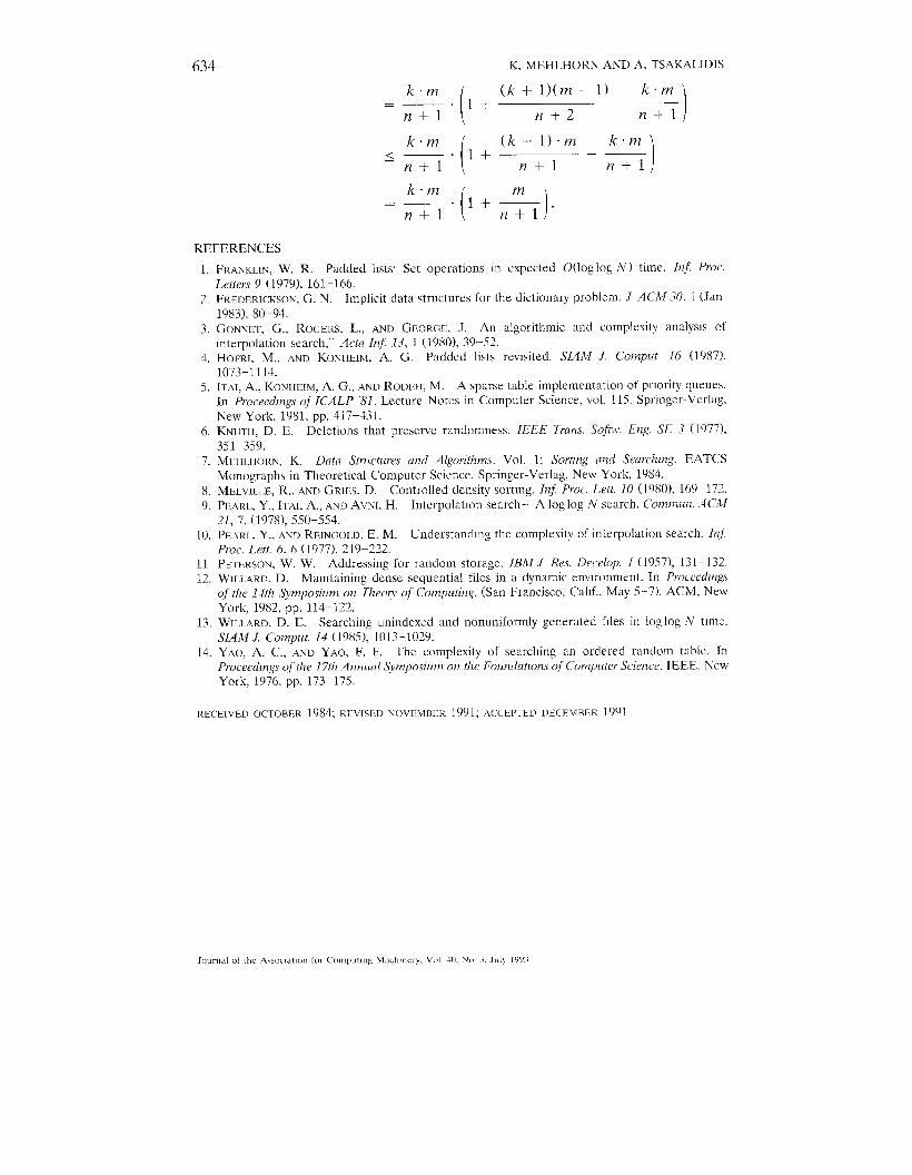
634 K. MEHLHORN AND A. TSAKALIDIS
km
(
(k + l)(m – 1) km=—.1+
n+l n+2 n+l 1
km . ~+(k+l)”m
(
k “ t?l<—
72+1 n+l n+l 1
k “ ttt
(
m.–—”l+—
n+l )72+1”
REFERENCES
1.
7-.
3.
4.
5.
6.
7.
8.9.
10.
1112
13
14
FRANKLIN, W. R. Padded hsts Set operations in expected O(log log N ) time. Inf Proc.
Letters 9 (1979), 161-166.
FREDERICIiSON, G. N. Implicit data structures for the dictionary problem. J .4CM 30, 1 (Jan
1983), 80-94.
GONNET, G., ROGERS, L., AND G~OR~E J. An algorithmic and complexity analyws ofinterpolation search,” Ackr Znf 13, 1 (1980), 39-52.
HOFRI, M., AND KON}lEIhf, A. G. Padded lists rewsited. SUM J. CornpUt 16 (1987),1073-1114.IT.AI, A., KONHEIM, A. G., .ANDRoDEti, M. A sparse table implementation of priority queues.
In Procecdzngs of’ ZCALP ’81. Lecture Notes in Computer Science, vol. 115. Springer-Verlag.
New York, 1981, pp. 417-431.KNUTH, D. E. Deletions that preserve randomness. IEEE Trans. Sofm. Eng. SE 3 (1977),
351-359.MEHLHORN, K. Data Structures and Algorithms. Vol. 1: Sorting and Searching. EATCS
Monographs in Theoretical Computer Science. Springer-Verlag, New York, 1984.
MELVILLE, R., ANDGRIES.D. Controlled density sorting. lnf. Proc. Lett. 10 (1980), 169-172.
PEARL, Y., ITAI, A., ANDAVNI, H. Interpolatmn search—A log log N search. Commun. ACM
?1, 7, (1978), 550–554.PEARL. Y., AND REINGOLD, E. M. Understanding the complexity of interpolation search. lnf.Proc. Left, 6.6 ( 1977), 219–222,
PETERSON, W. W. Addressing for random storage. IBM f Res. DeL’ehp. 1 (1957), 131-132.WILL.4RD, D. Maintaining dense sequential files in a dynamic enwronment. In Proceedings
of t;ze 14th Symposium on Theo~ of Computing. (San Francisco, Cahf., May 5–7). ACM, New
York, 1982, pp. 114-122.
WILLARD, D. E. Searching unindexed and nonuniformly generated fdes in log log N time.
SIAM /. COWIPU[.14 (1985), 1013-1029.YAO, A. C., AND YAO, F. F. The complexity of searching an ordered random table. InP~ocadmgs of the 17th .4 WILLC11Symposium OH the Fowz&ztzotzs of Computer Science. 1EEE, NewYork, 1976, pp. 173-175.
RECEIVED OCTOBER1984: RE\TSED NOVEMBER ] 991; .4zXEPTED DECEMBER 1991
Journal of the ASwLl~llon for Computtng M&hincry, 1’[,1 4(1, No 3. July 1993