Durham Research Online

Deposited in DRO:

12 February 2016

Version of attached �le:

Published Version

Peer-review status of attached �le:

Peer-reviewed

Citation for published item:

Allen, J. T. and Croom, S. M. and Konstantopoulos, I. S. and Bryant, J. J. and Sharp, R. and Cecil, G. N.and Fogarty, L. M. R. and Foster, C. and Green, A. W. and Ho, I.-T. and Owers, M. S. and Schaefer, A. L.and Scott, N. and Bauer, A. E. and Baldry, I. and Barnes, L. A. and Bland-Hawthorn, J. and Bloom, J. V.and Brough, S. and Colless, M. and Cortese, L. and Couch, W. J. and Drinkwater, M. J. and Driver, S. P. andGoodwin, M. and Gunawardhana, M. L. P. and Hampton, E. J. and Hopkins, A. M. and Kewley, L. J. andLawrence, J. S. and Leon-Saval, S. G. and Liske, J. and L�opez-S�anchez, �A. R. and Lorente, N. P. F. andMcElroy, R. and Medling, A. M. and Mould, J. and Norberg, P. and Parker, Q. A. and Power, C. and Pracy,M. B. and Richards, S. N. and Robotham, A. S. G. and Sweet, S. M. and Taylor, E. N. and Thomas, A. D.and Tonini, C. and Walcher, C. J. (2015) 'The SAMI Galaxy Survey : Early Data Release.', Monthly noticesof the Royal Astronomical Society., 446 (2). pp. 1567-1583.

Further information on publisher's website:

http://dx.doi.org/10.1093/mnras/stu2057

Publisher's copyright statement:

This article has been accepted for publication in Monthly Notices of the Royal Astronomical Society c©: 2014 The

Author Published by Oxford University Press on behalf of the Royal Astronomical Society. All rights reserved.

Additional information:

Use policy

The full-text may be used and/or reproduced, and given to third parties in any format or medium, without prior permission or charge, forpersonal research or study, educational, or not-for-pro�t purposes provided that:

• a full bibliographic reference is made to the original source

• a link is made to the metadata record in DRO

• the full-text is not changed in any way

The full-text must not be sold in any format or medium without the formal permission of the copyright holders.

Please consult the full DRO policy for further details.

Durham University Library, Stockton Road, Durham DH1 3LY, United KingdomTel : +44 (0)191 334 3042 | Fax : +44 (0)191 334 2971

http://dro.dur.ac.uk

MNRAS 446, 1567–1583 (2015) doi:10.1093/mnras/stu2057

The SAMI Galaxy Survey: Early Data Release

J. T. Allen,1,2‹ S. M. Croom,1,2 I. S. Konstantopoulos,2,3 J. J. Bryant,1,2,3 R. Sharp,4

G. N. Cecil,5 L. M. R. Fogarty,1,2 C. Foster,3 A. W. Green,3 I.-T. Ho,6 M. S. Owers,3

A. L. Schaefer,1,2,3 N. Scott,1,2 A. E. Bauer,3 I. Baldry,7 L. A. Barnes,1

J. Bland-Hawthorn,1,2 J. V. Bloom,1,2 S. Brough,3 M. Colless,4 L. Cortese,8

W. J. Couch,3 M. J. Drinkwater,9 S. P. Driver,10,11 M. Goodwin,3

M. L. P. Gunawardhana,12 E. J. Hampton,4 A. M. Hopkins,3 L. J. Kewley,4

J. S. Lawrence,3 S. G. Leon-Saval,13 J. Liske,14 A. R. Lopez-Sanchez,3,15

N. P. F. Lorente,3 R. McElroy,1,2 A. M. Medling,4 J. Mould,8 P. Norberg,12

Q. A. Parker,3,15,16 C. Power,2,10 M. B. Pracy,1 S. N. Richards,1,2,3

A. S. G. Robotham,10 S. M. Sweet,4,9 E. N. Taylor,17 A. D. Thomas,9 C. Tonini8

and C. J. Walcher18

Affiliations are listed at the end of the paper

Accepted 2014 September 30. Received 2014 September 30; in original form 2014 July 22

ABSTRACTWe present the Early Data Release of the Sydney–AAO Multi-object Integral field spectrograph(SAMI) Galaxy Survey. The SAMI Galaxy Survey is an ongoing integral field spectroscopicsurvey of ∼3400 low-redshift (z < 0.12) galaxies, covering galaxies in the field and in groupswithin the Galaxy And Mass Assembly (GAMA) survey regions, and a sample of galaxiesin clusters. In the Early Data Release, we publicly release the fully calibrated data cubesfor a representative selection of 107 galaxies drawn from the GAMA regions, along withinformation about these galaxies from the GAMA catalogues. All data cubes for the EarlyData Release galaxies can be downloaded individually or as a set from the SAMI GalaxySurvey website. In this paper we also assess the quality of the pipeline used to reduce theSAMI data, giving metrics that quantify its performance at all stages in processing the raw datainto calibrated data cubes. The pipeline gives excellent results throughout, with typical skysubtraction residuals in the continuum of 0.9–1.2 per cent, a relative flux calibration uncertaintyof 4.1 per cent (systematic) plus 4.3 per cent (statistical), and atmospheric dispersion removedwith an accuracy of 0.09 arcsec, less than a fifth of a spaxel.

Key words: techniques: imaging spectroscopy – galaxies: evolution – galaxies: kinematicsand dynamics – galaxies: structure.

1 IN T RO D U C T I O N

Spectroscopic surveys of galaxies – e.g. the 2-degree Field GalaxyRedshift Survey (2dFGRS; Colless et al. 2001), 6-degree FieldGalaxy Survey (6dFGS; Jones et al. 2009), Sloan Digital Sky Survey(SDSS; York et al. 2000) and Galaxy And Mass Assembly (GAMA;Driver et al. 2009, 2011) survey – are immensely powerful tools forinvestigating galaxy formation and evolution. Optical spectroscopy

� E-mail: j.allen@physics.usyd.edu.au

provides measurements of properties such as the star formation rate(SFR), stellar ages, metallicity of gas and stars, and dust extinction.Emission from other processes such as active galactic nuclei (AGN)and shock-heated gas is also measured. Multi-object spectrographshave allowed us to collate these properties for large samples ofgalaxies and search for correlations that illuminate the underlyingphysics of galaxy evolution, as well as find outliers that can beused to test models under the most extreme conditions. Surveysof this type have shed new light on the role of environment instar formation (e.g. Lewis et al. 2002; Wijesinghe et al. 2012),the relationship between supermassive black holes and their host

C© 2014 The AuthorsPublished by Oxford University Press on behalf of the Royal Astronomical Society

at University of D

urham on February 12, 2016

http://mnras.oxfordjournals.org/

Dow

nloaded from

1568 J. T. Allen et al.

galaxies (e.g. Shen et al. 2008), the mass–metallicity–SFR relation(e.g. Mannucci et al. 2010; Lara-Lopez et al. 2013) and many otheraspects of extragalactic astrophysics.

Notwithstanding the great achievements of traditional spectro-scopic surveys, the use of a single fibre or slit to observe eachgalaxy limits the available information. A clear example of thislimitation is that an SFR measured from a single spectrum must beaperture corrected to recover the global SFR, introducing an extrauncertainty (Hopkins et al. 2003). In many cases, the exact locationof the fibre or slit within the galaxy is not known, increasing theuncertainty from aperture effects. More critically, single-fibre ob-servations can only provide a single measurement of any propertyfor the entire galaxy, and so are inherently unable to probe spatialvariations in SFR, ionization state, stellar populations or any otherparameter. Similarly, they cannot provide any information about theinternal kinematics of the galaxy other than an integrated velocitydispersion.

These limitations are addressed by the use of spatially resolvedspectroscopy, based on integral field units (IFUs). Measuring thespatially resolved properties of galaxies has opened up a new di-rection in the study of galaxy evolution: studies of turbulent star-forming discs (Genzel et al. 2008), galactic winds from AGN andstar formation (Sharp & Bland-Hawthorn 2010), the environmentaldependence of stellar kinematics (Cappellari et al. 2011b) and starformation distributions (Brough et al. 2013), and age and metallic-ity gradients in stellar populations (Sanchez-Blazquez et al. 2014)provide only a small sample of the contributions of integral fieldspectroscopy.

Until now, technical limitations have meant that almost all IFUinstruments have been monolithic, viewing a single galaxy at atime. As a result, observing large numbers of galaxies has beendifficult and time-consuming. The largest samples of IFU obser-vations available to date have been the ATLAS-3D survey, with260 galaxies (Cappellari et al. 2011a), and the ongoing Calar AltoLegacy Integral Field Area (CALIFA) survey, with a target of 600galaxies (Sanchez et al. 2012). Surveys of this size are alreadybreaking new ground in our understanding of galaxy evolution, butwith monolithic IFUs they cannot be scaled up much further.

The next step forward for integral field spectroscopic surveysis to use multiplexed IFUs capable of observing multiple galaxiessimultaneously. The first such instrument, the Fibre Large ArrayMulti Element Spectrograph (FLAMES; Pasquini et al. 2002) onthe 8-m Very Large Telescope (VLT) has 15 deployable IFUs with20 spaxels (spatial elements) each and 2 × 3 arcsec2 fields of view.Despite the small number of spaxels in each IFU, FLAMES hasdemonstrated the power of multiplexed IFU systems, for exampleshowing the increased kinematic complexity of galaxies at mediumredshift (z ∼ 0.6; Flores et al. 2006; Yang et al. 2008).

For studies at low redshift (z < ∼0.2), IFUs with larger fieldsof view are required to probe the full extent of each galaxy.The Sydney–AAO Multi-object Integral field spectrograph (SAMI;Croom et al. 2012) on the 3.9-m Anglo-Australian Telescope (AAT)is the first instrument with this capability, having 13 IFUs each witha field of view of ≈15 arcsec. SAMI makes use of hexabundles,bundles of 61 fibres that are fused together and have a high opticalperformance and ∼75 per cent filling factor (Bland-Hawthorn et al.2011; Bryant et al. 2011, 2014a). The fibres feed into the existingAAOmega spectrograph (Sharp et al. 2006), a double-beamed spec-trograph that offers a range of configurations suitable for galaxyspectroscopy. Since its commissioning in 2012, SAMI observa-tions have been used for studies of galactic winds (Fogarty et al.2012; Ho et al. 2014), the kinematic morphology–density relation

(Fogarty et al. 2014) and star formation in dwarf galaxies (Richardset al. 2014).

The SAMI Galaxy Survey is an ongoing survey to observe ∼3400galaxies covering a wide range of stellar masses, redshifts, and en-vironmental densities. The science goals of the survey are broad,with key themes being the dependence of galaxy evolution on envi-ronment, and the build-up of galaxy mass and angular momentum.Observations began in 2013 March and are scheduled to continueuntil mid-2016.

We present here the Early Data Release (EDR) of the SAMIGalaxy Survey, containing fully calibrated data cubes and associ-ated catalogue information for 107 galaxies selected from the fullsample. The EDR sample is described in Section 2, and a briefoverview of the SAMI data reduction process is given in Section 3.We provide instructions for accessing and using the EDR data inSection 4. Section 5 presents a thorough analysis of the results fromthe SAMI data reduction pipeline, including key metrics that quan-tify its current performance. Finally, we summarize our findings inSection 6.

2 EARLY DATA R ELEASE SAMPLE

The targets for the SAMI Galaxy Survey are drawn from the GAMAsurvey G09, G12 and G15 fields, as well as a set of eight galaxyclusters that extend the survey to higher environmental densities. Allcandidates have known redshifts from GAMA, SDSS or dedicated2dF observations, allowing us to create a tiered set of volume-limited samples. Full details of the target selection are presented inBryant et al. (2014b).

The 107 galaxies that form the SAMI Galaxy Survey EDR arethose contained in nine fields in the GAMA regions that were ob-served in 2013 March and April. Each field contains 12 galaxies.One galaxy – GAMA ID 373248 – was observed in two separatefields. For this galaxy the EDR contains only the data from thefield in which the atmospheric seeing at the time of observation wasbetter (1.2 arcsec rather than 2.2 arcsec). The full list of galaxiesincluded in the EDR is given in Table A1, which contains detailedinformation about each galaxy.

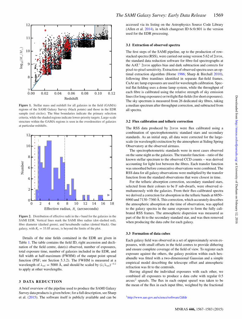
We manually selected the fields in the EDR to provide a repre-sentative subsample of the GAMA regions of the full SAMI GalaxySurvey, covering the range of redshifts, stellar masses and galaxymorphologies as completely as possible. The stellar masses (Tayloret al. 2011; Bryant et al. 2014b) and redshifts (Driver et al. 2011)of the EDR sample are shown in the context of the full survey inFig. 1, which also illustrates the survey’s selection criteria. TheEDR sample does not contain any galaxies from the high-redshiftfiller targets, or from the targets with the lowest mass and red-shift, resulting in slightly reduced ranges relative to the full sample:8.2 < log (M∗/M�) < 11.6 and 0.01 < z < 0.09.

Although no cut was made on the apparent size of the SAMIGalaxy Survey targets, the mass and redshift criteria were chosenwith the field of view and fibre size of the SAMI instrument in mind.Most of the galaxies in both the EDR and the full survey are smallenough that the field of view reaches at least one effective radius(Re), and large enough that SAMI can resolve their light across anumber of fibres. Fig. 2 shows the distribution of r-band major-axisRe, drawn from the GAMA analysis of SDSS imaging (Kelvin et al.2012), for the galaxies in the EDR. The median Re is 4.39 arcsec,with 17 of the 107 having Re greater than the radius of the SAMIhexabundles (7.5 arcsec). Only two galaxies have Re smaller thanthe fibre diameter (1.6 arcsec), and none have Re smaller than thefibre radius.

MNRAS 446, 1567–1583 (2015)

at University of D

urham on February 12, 2016

http://mnras.oxfordjournals.org/

Dow

nloaded from

The SAMI Galaxy Survey: Early Data Release 1569

Figure 1. Stellar mass and redshift for all galaxies in the field (GAMA)regions of the SAMI Galaxy Survey (black points) and those in the EDRsample (red circles). The blue boundaries indicate the primary selectioncriteria, while the shaded regions indicate lower-priority targets. Large-scalestructure within the GAMA regions is seen in the overdensities of galaxiesat particular redshifts.

Figure 2. Distribution of effective radii in the r band for the galaxies in theSAMI EDR. Vertical lines mark the SAMI fibre radius (dot–dashed red),fibre diameter (dashed green), and hexabundle radius (dotted black). Onegalaxy, with Re = 33.05 arcsec, is beyond the limits of the plot.

Details of the nine fields contained in the EDR are given inTable 1. The table contains the field ID, right ascension and decli-nation of the field centre, date(s) observed, number of exposures,total exposure time, number of galaxies included in the EDR, andfull width at half-maximum (FWHM) of the output point spreadfunction (PSF; see Section 5.3.2). The FWHM is measured at awavelength of λref = 5000 Å, and should be scaled by (λ/λref)−0.2

to apply at other wavelengths.

3 DATA R E D U C T I O N

A brief overview of the pipeline used to produce the SAMI GalaxySurvey data products is given below; for a full description, see Sharpet al. (2015). The software itself is publicly available and can be

accessed via its listing on the Astrophysics Source Code Library(Allen et al. 2014), in which changeset ID 6C0C801 is the versionused for the EDR processing.

3.1 Extraction of observed spectra

The first steps of the SAMI pipeline, up to the production of row-stacked spectra (RSS), were carried out using version 5.62 of 2DFDR,the standard data reduction software for fibre-fed spectrographs atthe AAT.1 2DFDR applies bias and dark subtraction and corrects forpixel-to-pixel sensitivity. Extraction of observed spectra uses an op-timal extraction algorithm (Horne 1986; Sharp & Birchall 2010),following fibre tramlines identified in separate flat-field frames.CuAr arc lamp exposures are used for wavelength calibration. Spec-tral flat fielding uses a dome lamp system, while the throughput ofeach fibre is calibrated using the relative strength of sky emissionlines (for long exposures) or twilight flat-fields (for short exposures).The sky spectrum is measured from 26 dedicated sky fibres, takinga median spectrum after throughput correction, and subtracted fromall spectra.

3.2 Flux calibration and telluric correction

The RSS data produced by 2DFDR were flux calibrated using acombination of spectrophotometric standard stars and secondarystandards. As an initial step, all data were corrected for the large-scale (in wavelength) extinction by the atmosphere at Siding SpringObservatory at the observed airmass.

The spectrophotometric standards were in most cases observedon the same night as the galaxies. The transfer function – ratio of theknown stellar spectrum to the observed CCD counts – was derivedaccounting for light lost between the fibres. Each transfer functionwas smoothed before consecutive observations were combined. TheRSS data for all galaxy observations were multiplied by the transferfunction from the standard observations that were closest in time.

For the telluric absorption correction, secondary standard stars,selected from their colours to be F sub-dwarfs, were observed si-multaneously with the galaxies. From their flux-calibrated spectrawe derived a correction for absorption in the telluric bands at 6850–6960 and 7130–7360 Å. This correction, which accurately describesthe atmospheric absorption at the time of observation, was appliedto the galaxy spectra in the same exposure to form the fully cali-brated RSS frames. The atmospheric dispersion was measured aspart of the fit to the secondary standard star, and was then removedwhen producing the data cube for each galaxy.

3.3 Formation of data cubes

Each galaxy field was observed in a set of approximately seven ex-posures, with small offsets in the field centres to provide ditheringand ensure complete coverage of the field of view. To register eachexposure against the others, the galaxy position within each hex-abundle was fitted with a two-dimensional Gaussian and a simpleempirical model describing the telescope offset and atmosphericrefraction was fit to the centroids.

Having aligned the individual exposures with each other, wecombined all exposures to produce a data cube with regular 0.5arcsec2 spaxels. The flux in each output spaxel was taken to bethe mean of the flux in each input fibre, weighted by the fractional

1http://www.aao.gov.au/science/software/2dfdr

MNRAS 446, 1567–1583 (2015)

at University of D

urham on February 12, 2016

http://mnras.oxfordjournals.org/

Dow

nloaded from

1570 J. T. Allen et al.

Table 1. Fields observed as part of the EDR. See text for a description of the columns. Coordinates are given in decimaldegrees at J2000 epoch.

Field ID RA (deg) Dec. (deg) Date(s) observed Nexp texp (s) Ngal FWHM (arcsec)

Y13SAR1 P003 09T006 140.1079 +1.2923 2013 Mar. 7 7 12 600 12 1.8Y13SAR1 P003 15T008 222.6946 −0.3410 2013 Mar. 7 7 12 600 12 2.1Y13SAR1 P005 09T009 131.6677 +2.2979 2013 Mar. 11 7 12 600 12 2.5Y13SAR1 P005 15T018 216.1500 −1.4587 2013 Mar. 11 8 14 400 12 2.4Y13SAR1 P008 09T013 132.5411 −0.0461 2013 Apr. 14, 16 7 12 600 12 1.8Y13SAR1 P009 09T015 139.9145 +0.9335 2013 Mar. 15 7 12 600 11 2.5Y13SAR1 P009 15T013 212.7953 −0.7502 2013 Mar. 15 7 12 600 12 1.9Y13SAR1 P014 12T001 181.0885 +1.7816 2013 Apr. 12, 13 7 12 600 12 2.2Y13SAR1 P014 15T029 214.1435 +0.1883 2013 Apr. 12 7 12 600 12 2.4

spatial overlap of that fibre with the spaxel. To regain some of thespatial resolution that would otherwise be lost in convolving the 1.6arcsec fibres with 0.5 arcsec spaxels, the overlaps were calculatedusing a fibre footprint with only 0.8 arcsec diameter (a drizzle-likeprocess; see Fruchter & Hook 2002; Sharp et al. 2015). The varianceinformation was fully propagated through the cubing process.

Because each input fibre overlaps with more than one outputspaxel, the flux measurements in the data cubes are covariant withnearby spaxels. This is a generic issue for any data that are resam-pled on to a grid; for example, Husemann et al. (2013) discuss theproblem in the context of the CALIFA survey. A crucial conse-quence is that, when spectra from two or more spaxels are summed,the variance of the summed spectrum is not equal to the sum of thevariances of the individual spectra. Similarly, a model fit to the datacube would need to account for the covariance between spaxels. Theformat in which the covariance information is stored is describedin Section 4.2 (further details are given in Sharp et al. 2015) and itseffect is quantified in Section 5.3.5.

The earlier flux calibration step assumed that the atmosphericconditions did not vary between the observations of the galaxiesand the spectrophotometric standard star. Although this is usuallya good approximation, the atmospheric transmission can vary dur-ing the night. These variations were measured by fitting a Moffatprofile to the data cube of the secondary standard star, extracting itsfull spectrum, then integrating across the SDSS g band to find theobserved flux. All objects in the field were then scaled by the ratioof the true flux of the star – from the SDSS or, for some clusterfields, VLT Survey Telescope (VST) ATLAS (Shanks et al. 2013)imaging catalogues – to the observed flux, under the assumptionthat the atmospheric variation is the same across the entire field.

4 DATA PRO D U C T S

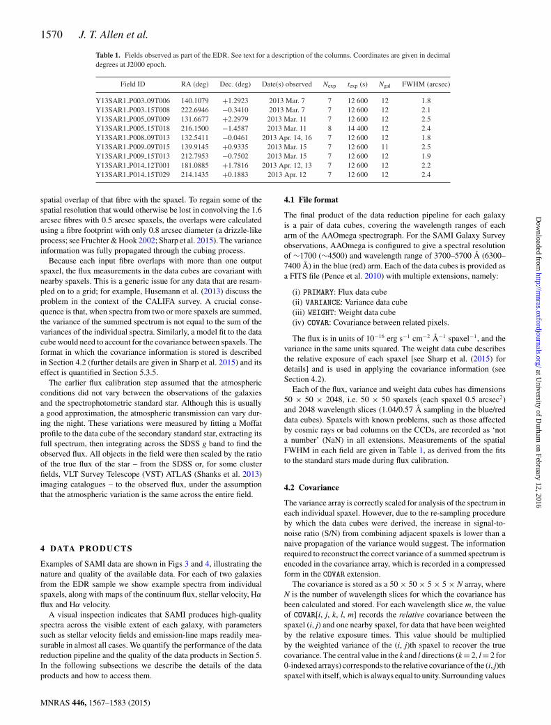
Examples of SAMI data are shown in Figs 3 and 4, illustrating thenature and quality of the available data. For each of two galaxiesfrom the EDR sample we show example spectra from individualspaxels, along with maps of the continuum flux, stellar velocity, Hα

flux and Hα velocity.A visual inspection indicates that SAMI produces high-quality

spectra across the visible extent of each galaxy, with parameterssuch as stellar velocity fields and emission-line maps readily mea-surable in almost all cases. We quantify the performance of the datareduction pipeline and the quality of the data products in Section 5.In the following subsections we describe the details of the dataproducts and how to access them.

4.1 File format

The final product of the data reduction pipeline for each galaxyis a pair of data cubes, covering the wavelength ranges of eacharm of the AAOmega spectrograph. For the SAMI Galaxy Surveyobservations, AAOmega is configured to give a spectral resolutionof ∼1700 (∼4500) and wavelength range of 3700–5700 Å (6300–7400 Å) in the blue (red) arm. Each of the data cubes is provided asa FITS file (Pence et al. 2010) with multiple extensions, namely:

(i) PRIMARY: Flux data cube(ii) VARIANCE: Variance data cube(iii) WEIGHT: Weight data cube(iv) COVAR: Covariance between related pixels.

The flux is in units of 10−16 erg s−1 cm−2 Å−1 spaxel−1, and thevariance in the same units squared. The weight data cube describesthe relative exposure of each spaxel [see Sharp et al. (2015) fordetails] and is used in applying the covariance information (seeSection 4.2).

Each of the flux, variance and weight data cubes has dimensions50 × 50 × 2048, i.e. 50 × 50 spaxels (each spaxel 0.5 arcsec2)and 2048 wavelength slices (1.04/0.57 Å sampling in the blue/reddata cubes). Spaxels with known problems, such as those affectedby cosmic rays or bad columns on the CCDs, are recorded as ‘nota number’ (NaN) in all extensions. Measurements of the spatialFWHM in each field are given in Table 1, as derived from the fitsto the standard stars made during flux calibration.

4.2 Covariance

The variance array is correctly scaled for analysis of the spectrum ineach individual spaxel. However, due to the re-sampling procedureby which the data cubes were derived, the increase in signal-to-noise ratio (S/N) from combining adjacent spaxels is lower than anaive propagation of the variance would suggest. The informationrequired to reconstruct the correct variance of a summed spectrum isencoded in the covariance array, which is recorded in a compressedform in the COVAR extension.

The covariance is stored as a 50 × 50 × 5 × 5 × N array, whereN is the number of wavelength slices for which the covariance hasbeen calculated and stored. For each wavelength slice m, the valueof COVAR[i, j, k, l, m] records the relative covariance between thespaxel (i, j) and one nearby spaxel, for data that have been weightedby the relative exposure times. This value should be multipliedby the weighted variance of the (i, j)th spaxel to recover the truecovariance. The central value in the k and l directions (k = 2, l = 2 for0-indexed arrays) corresponds to the relative covariance of the (i, j)thspaxel with itself, which is always equal to unity. Surrounding values

MNRAS 446, 1567–1583 (2015)

at University of D

urham on February 12, 2016

http://mnras.oxfordjournals.org/

Dow

nloaded from

The SAMI Galaxy Survey: Early Data Release 1571

Figure 3. Example SAMI data for the galaxy 511867, with z = 0.05523 and M∗ = 1010.68M�. Upper panel: flux for a central spaxel (blue) and one 3.75

arcsec to the North (red). Lower panels, from left to right: SDSS gri image; continuum flux map (10−16 erg s−1 cm−2 Å−1); stellar velocity field (km s−1);Hα flux map (10−16 erg s−1 cm−2); Hα velocity field (km s−1). The two velocity fields are each scaled individually. For the stellar velocity map, only spaxelswith per-pixel S/N >5 in the continuum are included. Each panel is 18 arcsec square, with North up and East to the left. The grey circle in the second panelshows the FWHM of the PSF.

Figure 4. As Fig. 3, for the galaxy 599761 with z = 0.05333 and M∗ = 1010.88M�.

MNRAS 446, 1567–1583 (2015)

at University of D

urham on February 12, 2016

http://mnras.oxfordjournals.org/

Dow

nloaded from

1572 J. T. Allen et al.

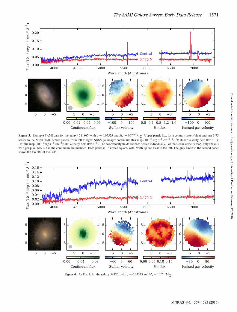
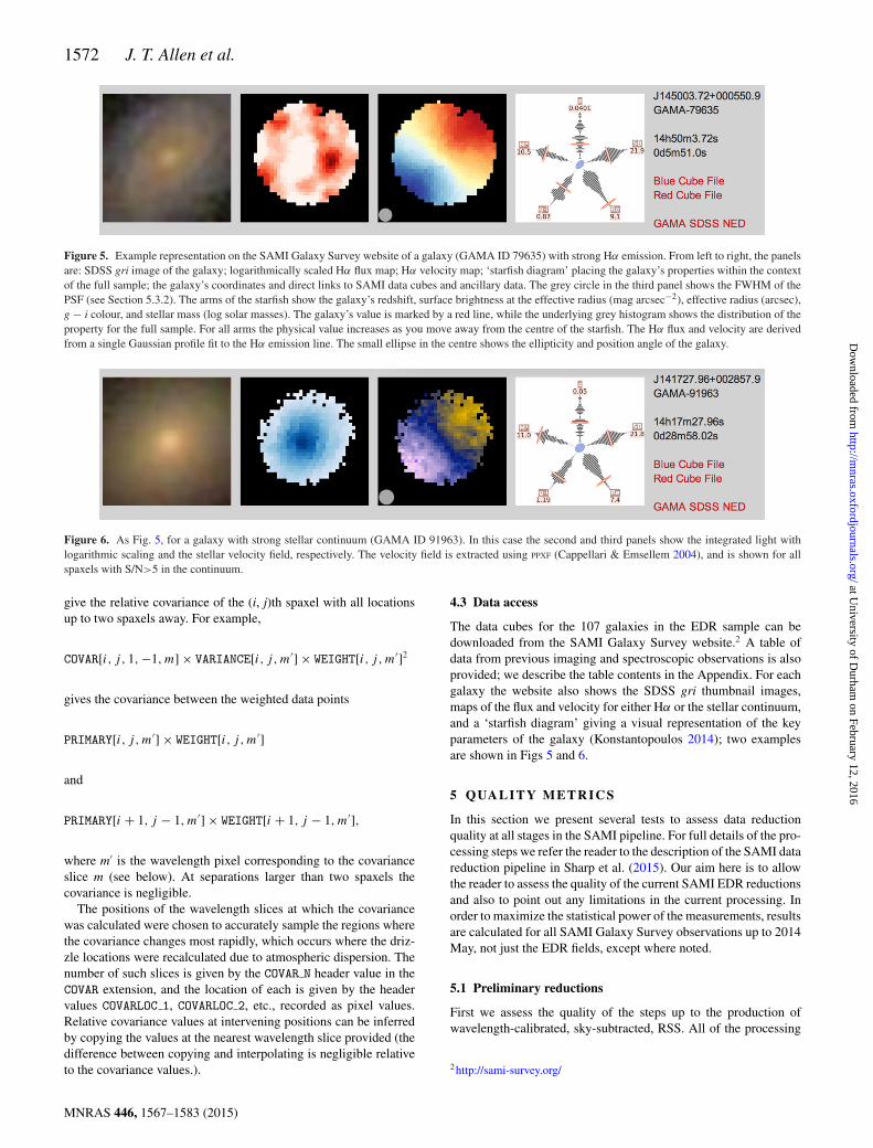
Figure 5. Example representation on the SAMI Galaxy Survey website of a galaxy (GAMA ID 79635) with strong Hα emission. From left to right, the panelsare: SDSS gri image of the galaxy; logarithmically scaled Hα flux map; Hα velocity map; ‘starfish diagram’ placing the galaxy’s properties within the contextof the full sample; the galaxy’s coordinates and direct links to SAMI data cubes and ancillary data. The grey circle in the third panel shows the FWHM of thePSF (see Section 5.3.2). The arms of the starfish show the galaxy’s redshift, surface brightness at the effective radius (mag arcsec−2), effective radius (arcsec),g − i colour, and stellar mass (log solar masses). The galaxy’s value is marked by a red line, while the underlying grey histogram shows the distribution of theproperty for the full sample. For all arms the physical value increases as you move away from the centre of the starfish. The Hα flux and velocity are derivedfrom a single Gaussian profile fit to the Hα emission line. The small ellipse in the centre shows the ellipticity and position angle of the galaxy.

Figure 6. As Fig. 5, for a galaxy with strong stellar continuum (GAMA ID 91963). In this case the second and third panels show the integrated light withlogarithmic scaling and the stellar velocity field, respectively. The velocity field is extracted using PPXF (Cappellari & Emsellem 2004), and is shown for allspaxels with S/N>5 in the continuum.

give the relative covariance of the (i, j)th spaxel with all locationsup to two spaxels away. For example,

COVAR[i, j , 1, −1, m] × VARIANCE[i, j , m′] × WEIGHT[i, j , m′]2

gives the covariance between the weighted data points

PRIMARY[i, j , m′] × WEIGHT[i, j , m′]

and

PRIMARY[i + 1, j − 1, m′] × WEIGHT[i + 1, j − 1, m′],

where m′ is the wavelength pixel corresponding to the covarianceslice m (see below). At separations larger than two spaxels thecovariance is negligible.

The positions of the wavelength slices at which the covariancewas calculated were chosen to accurately sample the regions wherethe covariance changes most rapidly, which occurs where the driz-zle locations were recalculated due to atmospheric dispersion. Thenumber of such slices is given by the COVAR N header value in theCOVAR extension, and the location of each is given by the headervalues COVARLOC 1, COVARLOC 2, etc., recorded as pixel values.Relative covariance values at intervening positions can be inferredby copying the values at the nearest wavelength slice provided (thedifference between copying and interpolating is negligible relativeto the covariance values.).

4.3 Data access

The data cubes for the 107 galaxies in the EDR sample can bedownloaded from the SAMI Galaxy Survey website.2 A table ofdata from previous imaging and spectroscopic observations is alsoprovided; we describe the table contents in the Appendix. For eachgalaxy the website also shows the SDSS gri thumbnail images,maps of the flux and velocity for either Hα or the stellar continuum,and a ‘starfish diagram’ giving a visual representation of the keyparameters of the galaxy (Konstantopoulos 2014); two examplesare shown in Figs 5 and 6.

5 QUA LI TY METRI CS

In this section we present several tests to assess data reductionquality at all stages in the SAMI pipeline. For full details of the pro-cessing steps we refer the reader to the description of the SAMI datareduction pipeline in Sharp et al. (2015). Our aim here is to allowthe reader to assess the quality of the current SAMI EDR reductionsand also to point out any limitations in the current processing. Inorder to maximize the statistical power of the measurements, resultsare calculated for all SAMI Galaxy Survey observations up to 2014May, not just the EDR fields, except where noted.

5.1 Preliminary reductions

First we assess the quality of the steps up to the production ofwavelength-calibrated, sky-subtracted, RSS. All of the processing

2http://sami-survey.org/

MNRAS 446, 1567–1583 (2015)

at University of D

urham on February 12, 2016

http://mnras.oxfordjournals.org/

Dow

nloaded from

The SAMI Galaxy Survey: Early Data Release 1573

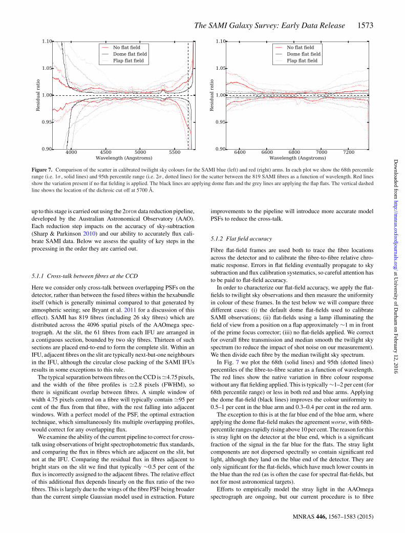
Figure 7. Comparison of the scatter in calibrated twilight sky colours for the SAMI blue (left) and red (right) arms. In each plot we show the 68th percentilerange (i.e. 1σ , solid lines) and 95th percentile range (i.e. 2σ , dotted lines) for the scatter between the 819 SAMI fibres as a function of wavelength. Red linesshow the variation present if no flat fielding is applied. The black lines are applying dome flats and the grey lines are applying the flap flats. The vertical dashedline shows the location of the dichroic cut off at 5700 Å.

up to this stage is carried out using the 2DFDR data reduction pipeline,developed by the Australian Astronomical Observatory (AAO).Each reduction step impacts on the accuracy of sky-subtraction(Sharp & Parkinson 2010) and our ability to accurately flux cali-brate SAMI data. Below we assess the quality of key steps in theprocessing in the order they are carried out.

5.1.1 Cross-talk between fibres at the CCD

Here we consider only cross-talk between overlapping PSFs on thedetector, rather than between the fused fibres within the hexabundleitself (which is generally minimal compared to that generated byatmospheric seeing; see Bryant et al. 2011 for a discussion of thiseffect). SAMI has 819 fibres (including 26 sky fibres) which aredistributed across the 4096 spatial pixels of the AAOmega spec-trograph. At the slit, the 61 fibres from each IFU are arranged ina contiguous section, bounded by two sky fibres. Thirteen of suchsections are placed end-to-end to form the complete slit. Within anIFU, adjacent fibres on the slit are typically next-but-one neighboursin the IFU, although the circular close packing of the SAMI IFUsresults in some exceptions to this rule.

The typical separation between fibres on the CCD is �4.75 pixels,and the width of the fibre profiles is �2.8 pixels (FWHM), sothere is significant overlap between fibres. A simple window ofwidth 4.75 pixels centred on a fibre will typically contain �95 percent of the flux from that fibre, with the rest falling into adjacentwindows. With a perfect model of the PSF, the optimal extractiontechnique, which simultaneously fits multiple overlapping profiles,would correct for any overlapping flux.

We examine the ability of the current pipeline to correct for cross-talk using observations of bright spectrophotometric flux standards,and comparing the flux in fibres which are adjacent on the slit, butnot at the IFU. Comparing the residual flux in fibres adjacent tobright stars on the slit we find that typically ∼0.5 per cent of theflux is incorrectly assigned to the adjacent fibres. The relative effectof this additional flux depends linearly on the flux ratio of the twofibres. This is largely due to the wings of the fibre PSF being broaderthan the current simple Gaussian model used in extraction. Future

improvements to the pipeline will introduce more accurate modelPSFs to reduce the cross-talk.

5.1.2 Flat field accuracy

Fibre flat-field frames are used both to trace the fibre locationsacross the detector and to calibrate the fibre-to-fibre relative chro-matic response. Errors in flat fielding eventually propagate to skysubtraction and flux calibration systematics, so careful attention hasto be paid to flat-field accuracy.

In order to characterize our flat-field accuracy, we apply the flat-fields to twilight sky observations and then measure the uniformityin colour of these frames. In the test below we will compare threedifferent cases: (i) the default dome flat-fields used to calibrateSAMI observations; (ii) flat-fields using a lamp illuminating thefield of view from a position on a flap approximately ∼1 m in frontof the prime focus corrector; (iii) no flat-fields applied. We correctfor overall fibre transmission and median smooth the twilight skyspectrum (to reduce the impact of shot noise on our measurement).We then divide each fibre by the median twilight sky spectrum.

In Fig. 7 we plot the 68th (solid lines) and 95th (dotted lines)percentiles of the fibre-to-fibre scatter as a function of wavelength.The red lines show the native variation in fibre colour responsewithout any flat fielding applied. This is typically ∼1–2 per cent (for68th percentile range) or less in both red and blue arms. Applyingthe dome flat-field (black lines) improves the colour uniformity to0.5–1 per cent in the blue arm and 0.3–0.4 per cent in the red arm.

The exception to this is at the far blue end of the blue arm, whereapplying the dome flat-field makes the agreement worse, with 68th-percentile ranges rapidly rising above 10 per cent. The reason for thisis stray light on the detector at the blue end, which is a significantfraction of the signal in the far blue for the flats. The stray lightcomponents are not dispersed spectrally so contain significant redlight, although they land on the blue end of the detector. They areonly significant for the flat-fields, which have much lower counts inthe blue than the red (as is often the case for spectral flat-fields, butnot for most astronomical targets).

Efforts to empirically model the stray light in the AAOmegaspectrograph are ongoing, but our current procedure is to fibre

MNRAS 446, 1567–1583 (2015)

at University of D

urham on February 12, 2016

http://mnras.oxfordjournals.org/

Dow

nloaded from

1574 J. T. Allen et al.

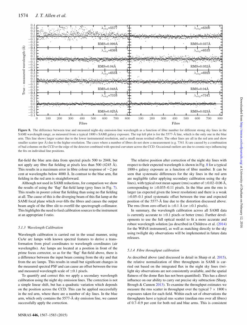
Figure 8. The difference between true and measured night-sky emission-line wavelength as a function of fibre number for different strong sky lines in theSAMI wavelength range, as measured from a typical 1800 s SAMI galaxy exposure. The top left plot is for the 5577-Å line, which is the only one in the bluearm. This line shows larger scatter due to the lower instrumental resolution, and a small mean residual offset. The other lines are all in the red arm and showsmaller scatter (per Å) due to the higher resolution. The cases where a number of fibres do not show a measurement (e.g. 7341 Å) are caused by a combinationof bad columns on the CCD or the edge of the detector combined with spectral curvature across the CCD. Occasional outliers are due to cosmic rays influencingthe fits on individual line positions.

flat-field the blue arm data from spectral pixels 500 to 2048, butnot apply any fibre flat fielding at pixels less than 500 (4245 Å).This results in a maximum error in fibre colour response of ∼2 percent at wavelengths below 4000 Å. In contrast to the blue arm, flatfielding in the red arm is straightforward.

Although not used in SAMI reductions, for comparison we showthe results of using the ‘flap’ flat-field lamp (grey lines in Fig. 7).This results in poorer colour flat fielding than using no flat fieldingat all. The cause of this is the diverging beam of this flat lamp at theSAMI focal plane which over-fills the fibres and causes the outputbeam angle of the fibre slit to overfill the spectrograph collimator.This highlights the need to feed calibration sources to the instrumentat an appropriate f-ratio.

5.1.3 Wavelength Calibration

Wavelength calibration is carried out in the usual manner, usingCuAr arc lamps with known spectral features to derive a trans-formation from pixel coordinates to wavelength coordinates (airwavelengths). Arc lamps are located at a position in front of theprime focus corrector, so as for the ‘flap’ flat-field above, there isa difference between the input beam coming from the sky and thatfrom the arc lamps. This results in small but significant changes inthe measured spectral PSF and can cause an offset between the trueand measured wavelength scale of �0.1 pixels.

To quantify and correct this we apply a secondary wavelengthcalibration using the night sky emission lines. The correction is nota simple linear shift, but has a quadratic variation which dependson the position across the CCD. This can be applied successfullyin the red arm, where there are a number of sky lines. In the bluearm, which only contains the 5577-Å sky emission line, we cannotsuccessfully apply the correction.

The relative position after correction of the night sky lines withrespect to their expected wavelength is shown in Fig. 8 for a typical1800-s galaxy exposure as a function of fibre number. It can beseen that systematic differences for the sky lines in the red armare negligible (after applying secondary calibration using the skylines), with typical root mean square (rms) scatter of �0.02–0.06 Å,corresponding to �0.035–0.11 pixels. In the blue arm the rms islarger (as expected given the lower resolution) and there is a weak�0.05–0.1 pixel systematic offset between the true and expectedposition of the 5577-Å line due to the distortion discussed above.The rms (from zero offset) is �0.1 Å (or �0.1 pixels).

In summary, the wavelength calibration across all SAMI datais currently accurate to �0.1 pixels or better (rms). Further devel-opments to use the full optical model to fit a more accurate androbust wavelength solution [as described in Childress et al. (2014)for the WiFeS instrument], as well as matching directly to the skyusing twilight sky observations will be implemented in future datareleases.

5.1.4 Fibre throughput calibration

As described above (and discussed in detail in Sharp et al. 2015),the relative normalization of fibre throughputs in SAMI is car-ried out based on the integrated flux in the night sky lines (twi-light sky observations are not consistently available, and the spatialflatness of the dome flats has not been quantified). This has a directinfluence on our ability to carry out precise sky subtraction (Sharp,Brough & Cannon 2013). To examine the throughput estimates wemeasure the rms scatter in throughput over the typical 7 × 1800 sexposures taken for each field. Within each set of observations thethroughputs have a typical rms scatter (median rms over all fibres)of 0.7–0.9 per cent for both red and blue arms. This is consistent

MNRAS 446, 1567–1583 (2015)

at University of D

urham on February 12, 2016

http://mnras.oxfordjournals.org/

Dow

nloaded from

The SAMI Galaxy Survey: Early Data Release 1575

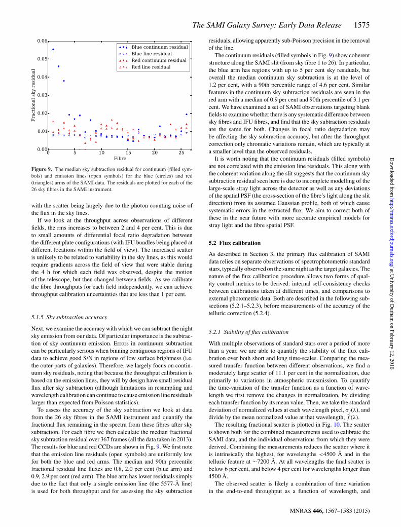
Figure 9. The median sky subtraction residual for continuum (filled sym-bols) and emission lines (open symbols) for the blue (circles) and red(triangles) arms of the SAMI data. The residuals are plotted for each of the26 sky fibres in the SAMI instrument.

with the scatter being largely due to the photon counting noise ofthe flux in the sky lines.

If we look at the throughput across observations of differentfields, the rms increases to between 2 and 4 per cent. This is dueto small amounts of differential focal ratio degradation betweenthe different plate configurations (with IFU bundles being placed atdifferent locations within the field of view). The increased scatteris unlikely to be related to variability in the sky lines, as this wouldrequire gradients across the field of view that were stable duringthe 4 h for which each field was observed, despite the motionof the telescope, but then changed between fields. As we calibratethe fibre throughputs for each field independently, we can achievethroughput calibration uncertainties that are less than 1 per cent.

5.1.5 Sky subtraction accuracy

Next, we examine the accuracy with which we can subtract the nightsky emission from our data. Of particular importance is the subtrac-tion of sky continuum emission. Errors in continuum subtractioncan be particularly serious when binning contiguous regions of IFUdata to achieve good S/N in regions of low surface brightness (i.e.the outer parts of galaxies). Therefore, we largely focus on contin-uum sky residuals, noting that because the throughput calibration isbased on the emission lines, they will by design have small residualflux after sky subtraction (although limitations in resampling andwavelength calibration can continue to cause emission line residualslarger than expected from Poisson statistics).

To assess the accuracy of the sky subtraction we look at datafrom the 26 sky fibres in the SAMI instrument and quantify thefractional flux remaining in the spectra from these fibres after skysubtraction. For each fibre we then calculate the median fractionalsky subtraction residual over 367 frames (all the data taken in 2013).The results for blue and red CCDs are shown in Fig. 9. We first notethat the emission line residuals (open symbols) are uniformly lowfor both the blue and red arms. The median and 90th percentilefractional residual line fluxes are 0.8, 2.0 per cent (blue arm) and0.9, 2.9 per cent (red arm). The blue arm has lower residuals simplydue to the fact that only a single emission line (the 5577-Å line)is used for both throughput and for assessing the sky subtraction

residuals, allowing apparently sub-Poisson precision in the removalof the line.

The continuum residuals (filled symbols in Fig. 9) show coherentstructure along the SAMI slit (from sky fibre 1 to 26). In particular,the blue arm has regions with up to 5 per cent sky residuals, butoverall the median continuum sky subtraction is at the level of1.2 per cent, with a 90th percentile range of 4.6 per cent. Similarfeatures in the continuum sky subtraction residuals are seen in thered arm with a median of 0.9 per cent and 90th percentile of 3.1 percent. We have examined a set of SAMI observations targeting blankfields to examine whether there is any systematic difference betweensky fibres and IFU fibres, and find that the sky subtraction residualsare the same for both. Changes in focal ratio degradation maybe affecting the sky subtraction accuracy, but after the throughputcorrection only chromatic variations remain, which are typically ata smaller level than the observed residuals.

It is worth noting that the continuum residuals (filled symbols)are not correlated with the emission line residuals. This along withthe coherent variation along the slit suggests that the continuum skysubtraction residual seen here is due to incomplete modelling of thelarge-scale stray light across the detector as well as any deviationsof the spatial PSF (the cross-section of the fibre’s light along the slitdirection) from its assumed Gaussian profile, both of which causesystematic errors in the extracted flux. We aim to correct both ofthese in the near future with more accurate empirical models forstray light and the fibre spatial PSF.

5.2 Flux calibration

As described in Section 3, the primary flux calibration of SAMIdata relies on separate observations of spectrophotometric standardstars, typically observed on the same night as the target galaxies. Thenature of the flux calibration procedure allows two forms of qual-ity control metrics to be derived: internal self-consistency checksbetween calibrations taken at different times, and comparisons toexternal photometric data. Both are described in the following sub-sections (5.2.1–5.2.3), before measurements of the accuracy of thetelluric correction (5.2.4).

5.2.1 Stability of flux calibration

With multiple observations of standard stars over a period of morethan a year, we are able to quantify the stability of the flux cali-bration over both short and long time-scales. Comparing the mea-sured transfer function between different observations, we find amoderately large scatter of 11.1 per cent in the normalization, dueprimarily to variations in atmospheric transmission. To quantifythe time-variation of the transfer function as a function of wave-length we first remove the changes in normalization, by dividingeach transfer function by its mean value. Then, we take the standarddeviation of normalized values at each wavelength pixel, σ f(λ), anddivide by the mean normalized value at that wavelength, f (λ).

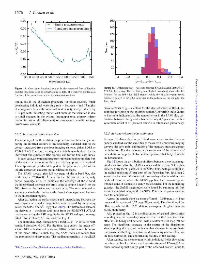
The resulting fractional scatter is plotted in Fig. 10. The scatteris shown both for the combined measurements used to calibrate theSAMI data, and the individual observations from which they werederived. Combining the measurements reduces the scatter where itis intrinsically the highest, for wavelengths <4500 Å and in thetelluric feature at ∼7200 Å. At all wavelengths the final scatter isbelow 6 per cent, and below 4 per cent for wavelengths longer than4500 Å.

The observed scatter is likely a combination of time variationin the end-to-end throughput as a function of wavelength, and

MNRAS 446, 1567–1583 (2015)

at University of D

urham on February 12, 2016

http://mnras.oxfordjournals.org/

Dow

nloaded from

1576 J. T. Allen et al.

Figure 10. One-sigma fractional scatter in the measured flux calibrationtransfer functions, over all observations to date. The scatter is plotted as afraction of the mean value across the same observations.

limitations in the extraction procedure for point sources. Whenconsidering individual observing runs – between 4 and 13 nightsof contiguous data – the observed scatter is typically reduced by∼30 per cent, indicating that at least some of the variation is dueto small changes in the system throughput (e.g. primary mirrorre-aluminization, slit alignment) or atmospheric conditions (e.g.dust/aerosol content).

5.2.2 Accuracy of colour correction

The accuracy of the flux calibration procedure can be seen by com-paring the inferred colours of the secondary standard stars to thecolours measured from previous imaging surveys, either SDSS orVST-ATLAS. There are two stages at which this can be done: for theindividual flux-calibrated RSS frames, and for the final data cubes.

In each case, an extracted spectrum representing the complete fluxof the star – i.e. accounting for the spatial sampling – is required.These spectra are produced as part of the pipeline, as part of thetelluric correction and zero-point calibration steps.

The SAMI spectra give full coverage of the g band but, dueto the gap at 5700–6300 Å between the blue and red arms, onlypartial coverage of r. To complete the coverage of the r band,we interpolated between the arms using a simple linear fit to the300 pixels at the inside end of each arm. The stars selected assecondary standards, F sub-dwarfs, do not show significant featuresin the interpolated region.

After extracting the stellar spectra and interpolating between thearms, synthetic g and r magnitudes were derived by integratingacross the SDSS filters3 (Hogg et al. 2002). The differences betweenthe derived g − r colours and those from the SDSS/VST-ATLAScatalogues, using the PSF magnitudes for SDSS and aperture mag-nitudes for VST-ATLAS, are shown in Fig. 11.

The individual RSS frames have a mean �(g − r) of 0.043 withstandard deviation 0.040. For the final data cubes, the mean off-set is 0.043 with standard deviation 0.046. In both cases the senseof the mean offset is such that the SAMI data are redder thanthe photometric observations. The median uncertainty in the SDSS

3http://www.sdss2.org/dr7/instruments/imager/index.html#filters

Figure 11. Difference in g − r colours between SAMI data and SDSS/VST-ATLAS photometry. The red histogram (dashed boundary) shows the dif-ferences for the individual RSS frames, while the blue histogram (solidboundary; scaled to have the same area as the red) shows the same for thedata cubes.

measurements of g − r colour for the stars observed is 0.024, ac-counting for some of the observed scatter. Converting these valuesto flux units indicates that the random error in the SAMI flux cal-ibration between the g and r bands is only 4.3 per cent, with asystematic offset of 4.1 per cent relative to established photometry.

5.2.3 Accuracy of zero-point calibration

Because the data cubes in each field were scaled to give the sec-ondary standard star the same flux as measured by previous imagingsurveys, the zero-point calibration of the standard stars are correctby definition. For the galaxies, a measurement of the accuracy ofthe calibration is possible for smaller galaxies that fully fit insidethe hexabundle.

Fig. 12 shows the distribution of offsets between the g-band mag-nitudes measured for the SAMI galaxies and those from SDSS pho-tometry. Only the 93 galaxies in the SDSS fields with petroR50 r,the radius enclosing 50 per cent of the Petrosian flux, less than 2arcsec are included. Galaxies with secondary objects within theirfields of view, or where the SDSS pipeline had erroneously at-tributed some of its flux to a star, were discarded. For the remaininggalaxies, the SAMI magnitudes were found by summing all fluxwithin the field of view, while the SDSS Petrosian magnitudes wereused for comparison.

Across the sample there is a mean offset of −0.049 mag (−4.4 percent) and 1σ scatter of 0.27 mag (28 per cent). The direction of theoffset is such that the SAMI data on average are brighter than theSDSS photometry.

Also plotted in Fig. 12 is the distribution of g-band offsets priorto scaling via the secondary standard star. In this case the meanoffset is 0.026 mag (2.4 per cent) with a scatter of 0.44 mag (50 percent). The significant decrease in the scatter of the distributionafter applying this scaling indicates that changes in atmospherictransmission affecting the entire field have a significant effect onthe flux calibration, and confirms the validity of the scaling.

After scaling, the mean scatter within individual fields (includingonly those with at least three small galaxies) is only 0.12 mag (12 percent), indicating that a large part of the observed scatter is due to

MNRAS 446, 1567–1583 (2015)

at University of D

urham on February 12, 2016

http://mnras.oxfordjournals.org/

Dow

nloaded from

The SAMI Galaxy Survey: Early Data Release 1577

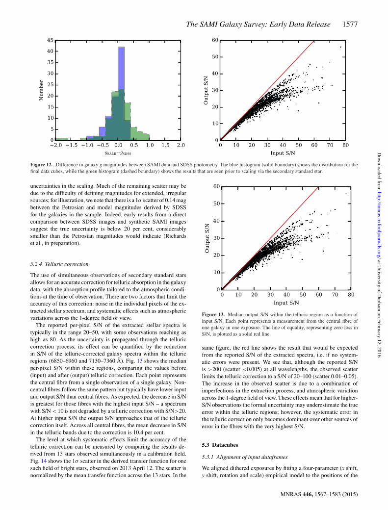
Figure 12. Difference in galaxy g magnitudes between SAMI data and SDSS photometry. The blue histogram (solid boundary) shows the distribution for thefinal data cubes, while the green histogram (dashed boundary) shows the results that are seen prior to scaling via the secondary standard star.

uncertainties in the scaling. Much of the remaining scatter may bedue to the difficulty of defining magnitudes for extended, irregularsources; for illustration, we note that there is a 1σ scatter of 0.14 magbetween the Petrosian and model magnitudes derived by SDSSfor the galaxies in the sample. Indeed, early results from a directcomparison between SDSS images and synthetic SAMI imagessuggest the true uncertainty is below 20 per cent, considerablysmaller than the Petrosian magnitudes would indicate (Richardset al., in preparation).

5.2.4 Telluric correction

The use of simultaneous observations of secondary standard starsallows for an accurate correction for telluric absorption in the galaxydata, with the absorption profile tailored to the atmospheric condi-tions at the time of observation. There are two factors that limit theaccuracy of this correction: noise in the individual pixels of the ex-tracted stellar spectrum, and systematic effects such as atmosphericvariations across the 1-degree field of view.

The reported per-pixel S/N of the extracted stellar spectra istypically in the range 20–50, with some observations reaching ashigh as 80. As the uncertainty is propagated through the telluriccorrection process, its effect can be quantified by the reductionin S/N of the telluric-corrected galaxy spectra within the telluricregions (6850–6960 and 7130–7360 Å). Fig. 13 shows the medianper-pixel S/N within these regions, comparing the values before(input) and after (output) telluric correction. Each point representsthe central fibre from a single observation of a single galaxy. Non-central fibres follow the same pattern but typically have lower inputand output S/N than central fibres. As expected, the decrease in S/Nis greatest for those fibres with the highest input S/N – a spectrumwith S/N < 10 is not degraded by a telluric correction with S/N>20.At higher input S/N the output S/N approaches that of the telluriccorrection itself. Across all central fibres, the mean decrease in S/Nin the telluric bands due to the correction is 10.4 per cent.

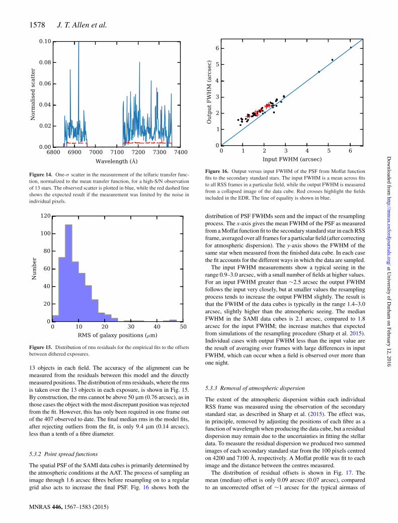
The level at which systematic effects limit the accuracy of thetelluric correction can be measured by comparing the results de-rived from 13 stars observed simultaneously in a calibration field.Fig. 14 shows the 1σ scatter in the derived transfer function for onesuch field of bright stars, observed on 2013 April 12. The scatter isnormalized by the mean transfer function across the 13 stars. In the

Figure 13. Median output S/N within the telluric region as a function ofinput S/N. Each point represents a measurement from the central fibre ofone galaxy in one exposure. The line of equality, representing zero loss inS/N, is plotted as a solid red line.

same figure, the red line shows the result that would be expectedfrom the reported S/N of the extracted spectra, i.e. if no system-atic errors were present. We see that, although the reported S/Nis >200 (scatter <0.005) at all wavelengths, the observed scatterlimits the telluric correction to a S/N of 20–100 (scatter 0.01–0.05).The increase in the observed scatter is due to a combination ofimperfections in the extraction process, and atmospheric variationacross the 1-degree field of view. These effects mean that for higher-S/N observations the formal uncertainty may underestimate the trueerror within the telluric regions; however, the systematic error inthe telluric correction only becomes dominant over other sources oferror in the fibres with the very highest S/N.

5.3 Datacubes

5.3.1 Alignment of input dataframes

We aligned dithered exposures by fitting a four-parameter (x shift,y shift, rotation and scale) empirical model to the positions of the

MNRAS 446, 1567–1583 (2015)

at University of D

urham on February 12, 2016

http://mnras.oxfordjournals.org/

Dow

nloaded from

1578 J. T. Allen et al.

Figure 14. One-σ scatter in the measurement of the telluric transfer func-tion, normalized to the mean transfer function, for a high-S/N observationof 13 stars. The observed scatter is plotted in blue, while the red dashed lineshows the expected result if the measurement was limited by the noise inindividual pixels.

Figure 15. Distribution of rms residuals for the empirical fits to the offsetsbetween dithered exposures.

13 objects in each field. The accuracy of the alignment can bemeasured from the residuals between this model and the directlymeasured positions. The distribution of rms residuals, where the rmsis taken over the 13 objects in each exposure, is shown in Fig. 15.By construction, the rms cannot be above 50 µm (0.76 arcsec), as inthose cases the object with the most discrepant position was rejectedfrom the fit. However, this has only been required in one frame outof the 407 observed to date. The final median rms in the model fits,after rejecting outliers from the fit, is only 9.4 µm (0.14 arcsec),less than a tenth of a fibre diameter.

5.3.2 Point spread functions

The spatial PSF of the SAMI data cubes is primarily determined bythe atmospheric conditions at the AAT. The process of sampling animage through 1.6 arcsec fibres before resampling on to a regulargrid also acts to increase the final PSF. Fig. 16 shows both the

Figure 16. Output versus input FWHM of the PSF from Moffat functionfits to the secondary standard stars. The input FWHM is a mean across fitsto all RSS frames in a particular field, while the output FWHM is measuredfrom a collapsed image of the data cube. Red crosses highlight the fieldsincluded in the EDR. The line of equality is shown in blue.

distribution of PSF FWHMs seen and the impact of the resamplingprocess. The x-axis gives the mean FWHM of the PSF as measuredfrom a Moffat function fit to the secondary standard star in each RSSframe, averaged over all frames for a particular field (after correctingfor atmospheric dispersion). The y-axis shows the FWHM of thesame star when measured from the finished data cube. In each casethe fit accounts for the different ways in which the data are sampled.

The input FWHM measurements show a typical seeing in therange 0.9–3.0 arcsec, with a small number of fields at higher values.For an input FWHM greater than ∼2.5 arcsec the output FWHMfollows the input very closely, but at smaller values the resamplingprocess tends to increase the output FWHM slightly. The result isthat the FWHM of the data cubes is typically in the range 1.4–3.0arcsec, slightly higher than the atmospheric seeing. The medianFWHM in the SAMI data cubes is 2.1 arcsec, compared to 1.8arcsec for the input FWHM; the increase matches that expectedfrom simulations of the resampling procedure (Sharp et al. 2015).Individual cases with output FWHM less than the input value arethe result of averaging over frames with large differences in inputFWHM, which can occur when a field is observed over more thanone night.

5.3.3 Removal of atmospheric dispersion

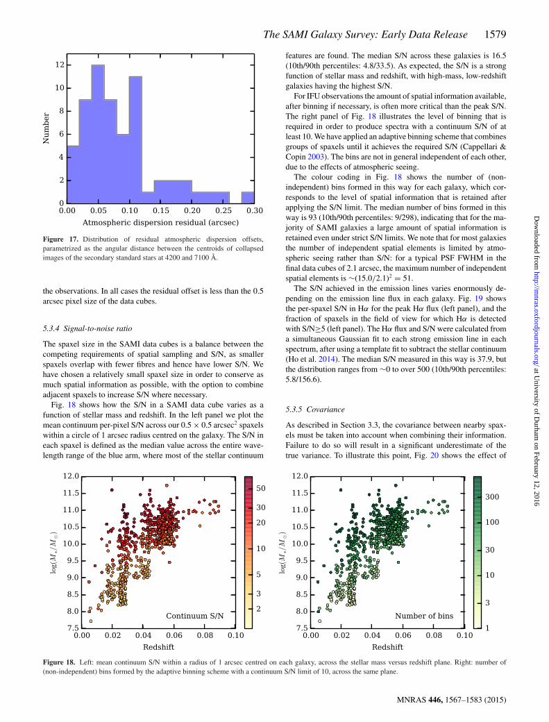
The extent of the atmospheric dispersion within each individualRSS frame was measured using the observation of the secondarystandard star, as described in Sharp et al. (2015). The effect was,in principle, removed by adjusting the positions of each fibre as afunction of wavelength when producing the data cube, but a residualdispersion may remain due to the uncertainties in fitting the stellardata. To measure the residual dispersion we produced two summedimages of each secondary standard star from the 100 pixels centredon 4200 and 7100 Å, respectively. A Moffat profile was fit to eachimage and the distance between the centres measured.

The distribution of residual offsets is shown in Fig. 17. Themean (median) offset is only 0.09 arcsec (0.07 arcsec), comparedto an uncorrected offset of ∼1 arcsec for the typical airmass of

MNRAS 446, 1567–1583 (2015)

at University of D

urham on February 12, 2016

http://mnras.oxfordjournals.org/

Dow

nloaded from

The SAMI Galaxy Survey: Early Data Release 1579

Figure 17. Distribution of residual atmospheric dispersion offsets,parametrized as the angular distance between the centroids of collapsedimages of the secondary standard stars at 4200 and 7100 Å.

the observations. In all cases the residual offset is less than the 0.5arcsec pixel size of the data cubes.

5.3.4 Signal-to-noise ratio

The spaxel size in the SAMI data cubes is a balance between thecompeting requirements of spatial sampling and S/N, as smallerspaxels overlap with fewer fibres and hence have lower S/N. Wehave chosen a relatively small spaxel size in order to conserve asmuch spatial information as possible, with the option to combineadjacent spaxels to increase S/N where necessary.

Fig. 18 shows how the S/N in a SAMI data cube varies as afunction of stellar mass and redshift. In the left panel we plot themean continuum per-pixel S/N across our 0.5 × 0.5 arcsec2 spaxelswithin a circle of 1 arcsec radius centred on the galaxy. The S/N ineach spaxel is defined as the median value across the entire wave-length range of the blue arm, where most of the stellar continuum

features are found. The median S/N across these galaxies is 16.5(10th/90th percentiles: 4.8/33.5). As expected, the S/N is a strongfunction of stellar mass and redshift, with high-mass, low-redshiftgalaxies having the highest S/N.

For IFU observations the amount of spatial information available,after binning if necessary, is often more critical than the peak S/N.The right panel of Fig. 18 illustrates the level of binning that isrequired in order to produce spectra with a continuum S/N of atleast 10. We have applied an adaptive binning scheme that combinesgroups of spaxels until it achieves the required S/N (Cappellari &Copin 2003). The bins are not in general independent of each other,due to the effects of atmospheric seeing.

The colour coding in Fig. 18 shows the number of (non-independent) bins formed in this way for each galaxy, which cor-responds to the level of spatial information that is retained afterapplying the S/N limit. The median number of bins formed in thisway is 93 (10th/90th percentiles: 9/298), indicating that for the ma-jority of SAMI galaxies a large amount of spatial information isretained even under strict S/N limits. We note that for most galaxiesthe number of independent spatial elements is limited by atmo-spheric seeing rather than S/N: for a typical PSF FWHM in thefinal data cubes of 2.1 arcsec, the maximum number of independentspatial elements is ∼(15.0/2.1)2 = 51.

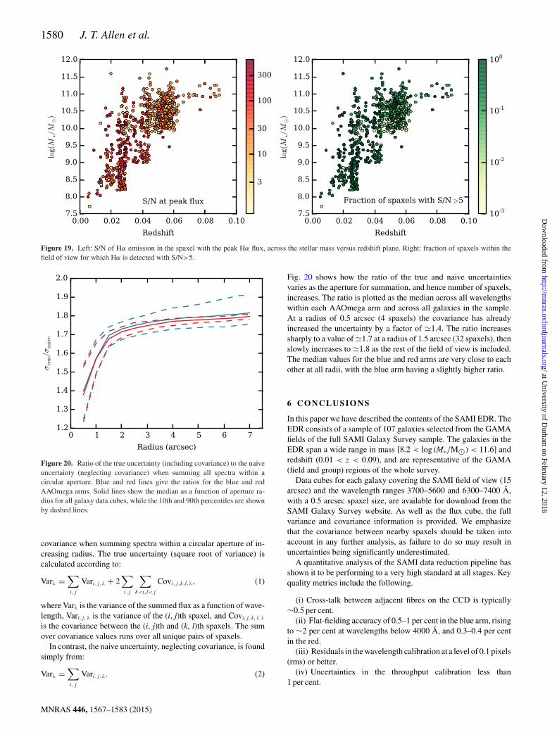
The S/N achieved in the emission lines varies enormously de-pending on the emission line flux in each galaxy. Fig. 19 showsthe per-spaxel S/N in Hα for the peak Hα flux (left panel), and thefraction of spaxels in the field of view for which Hα is detectedwith S/N≥5 (left panel). The Hα flux and S/N were calculated froma simultaneous Gaussian fit to each strong emission line in eachspectrum, after using a template fit to subtract the stellar continuum(Ho et al. 2014). The median S/N measured in this way is 37.9, butthe distribution ranges from ∼0 to over 500 (10th/90th percentiles:5.8/156.6).

5.3.5 Covariance

As described in Section 3.3, the covariance between nearby spax-els must be taken into account when combining their information.Failure to do so will result in a significant underestimate of thetrue variance. To illustrate this point, Fig. 20 shows the effect of

Figure 18. Left: mean continuum S/N within a radius of 1 arcsec centred on each galaxy, across the stellar mass versus redshift plane. Right: number of(non-independent) bins formed by the adaptive binning scheme with a continuum S/N limit of 10, across the same plane.

MNRAS 446, 1567–1583 (2015)

at University of D

urham on February 12, 2016

http://mnras.oxfordjournals.org/

Dow

nloaded from

1580 J. T. Allen et al.

Figure 19. Left: S/N of Hα emission in the spaxel with the peak Hα flux, across the stellar mass versus redshift plane. Right: fraction of spaxels within thefield of view for which Hα is detected with S/N>5.

Figure 20. Ratio of the true uncertainty (including covariance) to the naiveuncertainty (neglecting covariance) when summing all spectra within acircular aperture. Blue and red lines give the ratios for the blue and redAAOmega arms. Solid lines show the median as a function of aperture ra-dius for all galaxy data cubes, while the 10th and 90th percentiles are shownby dashed lines.

covariance when summing spectra within a circular aperture of in-creasing radius. The true uncertainty (square root of variance) iscalculated according to:

Varλ =∑

i,j

Vari,j ,λ + 2∑

i,j

∑

k<i,l<j

Covi,j ,k,l,λ, (1)

where Varλ is the variance of the summed flux as a function of wave-length, Vari, j, λ is the variance of the (i, j)th spaxel, and Covi, j, k, l, λ

is the covariance between the (i, j)th and (k, l)th spaxels. The sumover covariance values runs over all unique pairs of spaxels.

In contrast, the naive uncertainty, neglecting covariance, is foundsimply from:

Varλ =∑

i,j

Vari,j ,λ. (2)

Fig. 20 shows how the ratio of the true and naive uncertaintiesvaries as the aperture for summation, and hence number of spaxels,increases. The ratio is plotted as the median across all wavelengthswithin each AAOmega arm and across all galaxies in the sample.At a radius of 0.5 arcsec (4 spaxels) the covariance has alreadyincreased the uncertainty by a factor of �1.4. The ratio increasessharply to a value of �1.7 at a radius of 1.5 arcsec (32 spaxels), thenslowly increases to �1.8 as the rest of the field of view is included.The median values for the blue and red arms are very close to eachother at all radii, with the blue arm having a slightly higher ratio.

6 C O N C L U S I O N S

In this paper we have described the contents of the SAMI EDR. TheEDR consists of a sample of 107 galaxies selected from the GAMAfields of the full SAMI Galaxy Survey sample. The galaxies in theEDR span a wide range in mass [8.2 < log (M∗/M�) < 11.6] andredshift (0.01 < z < 0.09), and are representative of the GAMA(field and group) regions of the whole survey.

Data cubes for each galaxy covering the SAMI field of view (15arcsec) and the wavelength ranges 3700–5600 and 6300–7400 Å,with a 0.5 arcsec spaxel size, are available for download from theSAMI Galaxy Survey website. As well as the flux cube, the fullvariance and covariance information is provided. We emphasizethat the covariance between nearby spaxels should be taken intoaccount in any further analysis, as failure to do so may result inuncertainties being significantly underestimated.

A quantitative analysis of the SAMI data reduction pipeline hasshown it to be performing to a very high standard at all stages. Keyquality metrics include the following.

(i) Cross-talk between adjacent fibres on the CCD is typically∼0.5 per cent.

(ii) Flat-fielding accuracy of 0.5–1 per cent in the blue arm, risingto ∼2 per cent at wavelengths below 4000 Å, and 0.3–0.4 per centin the red.

(iii) Residuals in the wavelength calibration at a level of 0.1 pixels(rms) or better.

(iv) Uncertainties in the throughput calibration less than1 per cent.

MNRAS 446, 1567–1583 (2015)

at University of D

urham on February 12, 2016

http://mnras.oxfordjournals.org/

Dow

nloaded from

The SAMI Galaxy Survey: Early Data Release 1581

(v) After sky subtraction, median residual sky line fluxes of0.8 per cent (blue arm) and 0.9 per cent (red arm), relative to theunsubtracted flux.

(vi) Continuum residuals are typically 1.2 per cent (blue arm)and 0.9 per cent (red arm) of the sky level, rising to ∼5 per cent insome fibres.

(vii) In terms of the g − r colour, flux calibration that agrees withexisting photometric catalogues to within 4.3 per cent, with a meanoffset of 4.1 per cent (with the SAMI observations being redder).

(viii) An absolute flux calibration with a mean offset of 4.4 percent (with the SAMI observations being brighter) relative to SDSSphotometry, with a scatter of 28 per cent, although the true uncer-tainty may be considerably smaller.

(ix) Multiple dithered exposures for each field are aligned with amedian accuracy of 9.4 µm, less than a tenth of a fibre diameter.

(x) The observed PSF in the final data cubes is primarily deter-mined by the atmospheric conditions, with a median seeing FWHMof 2.1 arcsec.

(xi) The effects of atmospheric dispersion removed from the datacubes with a mean residual between images at different wavelengthsof 0.09 arcsec.

(xii) A median per-pixel continuum S/N in the central 0.5 × 0.5arcsec2 spaxels of 16.5, with 10th/90th percentiles of 4.8/33.5.

AC K N OW L E D G E M E N T S

We thank the referee for a number of useful suggestions that im-proved the quality of this work.

The SAMI Galaxy Survey is based on observations made at theAAT. The Sydney-AAO Multi-object Integral field spectrograph(SAMI) was developed jointly by the University of Sydney and theAAO. The SAMI input catalogue is based on data taken from theSDSS, the GAMA Survey and the VST ATLAS Survey. The SAMIGalaxy Survey is funded by the Australian Research Council Cen-tre of Excellence for All-sky Astrophysics (CAASTRO), throughproject number CE110001020, and other participating institutions.The SAMI Galaxy Survey website is http://sami-survey.org/.

GAMA is a joint European–Australasian project based arounda spectroscopic campaign using the AAT. The GAMA input cata-logue is based on data taken from the SDSS and the UKIRT In-frared Deep Sky Survey. Complementary imaging of the GAMAregions is being obtained by a number of independent survey pro-grams including GALEX MIS, VST KiDS, VISTA VIKING, WISE,Herschel-ATLAS, GMRT and ASKAP providing UV to radio cov-erage. GAMA is funded by the STFC (UK), the ARC (Australia),the AAO, and the participating institutions. The GAMA website ishttp://www.gama-survey.org/.

JTA acknowledges the award of an Australian Research Council(ARC) Super Science Fellowship (FS110200013). SMC acknowl-edges the support of an ARC Future Fellowship (FT100100457).ISK is the recipient of a John Stocker Postdoctoral Fellowship fromthe Science and Industry Endowment Fund (Australia). MSO ac-knowledges the funding support from the ARC through a SuperScience Fellowship (FS110200023). LC acknowledges support un-der the ARC Discovery Projects funding scheme (DP130100664).

This research made use of Astropy, a community-developed corePython package for Astronomy (Astropy Collaboration et al. 2013).

R E F E R E N C E S

Allen J. T. et al., 2014, Astrophysics Source Code Library (ascl:1407.006)Astropy Collaboration et al., 2013, A&A, 558, A33

Baldry I. K. et al., 2012, MNRAS, 421, 621Bland-Hawthorn J. et al., 2011, Opt. Express, 19, 2649Brough S. et al., 2013, MNRAS, 435, 2903Bryant J. J., O’Byrne J. W., Bland-Hawthorn J., Leon-Saval S. G., 2011,

MNRAS, 415, 2173Bryant J. J., Bland-Hawthorn J., Fogarty L. M. R., Lawrence J. S., Croom

S. M., 2014a, MNRAS, 438, 869Bryant J. J. et al., 2014b, MNRAS, submitted (arXiv:1407.7335)Cappellari M., Copin Y., 2003, MNRAS, 342, 345Cappellari M., Emsellem E., 2004, PASP, 116, 138Cappellari M. et al., 2011a, MNRAS, 413, 813Cappellari M. et al., 2011b, MNRAS, 416, 1680Childress M. J., Vogt F. P. A., Nielsen J., Sharp R. G., 2014, Astrophys.

Space Sci., 349, 617Colless M. et al., 2001, MNRAS, 328, 1039Croom S. M. et al., 2012, MNRAS, 421, 872Driver S. P. et al., 2009, Astron. Geophys., 50, 12Driver S. P. et al., 2011, MNRAS, 413, 971Flores H., Hammer F., Puech M., Amram P., Balkowski C., 2006, A&A,

455, 107Fogarty L. M. R. et al., 2012, ApJ, 761, 169Fogarty L. M. R. et al., 2014, MNRAS, 443, 485Fruchter A. S., Hook R. N., 2002, PASP, 114, 144Genzel R. et al., 2008, ApJ, 687, 59Hill D. T. et al., 2011, MNRAS, 412, 765Ho I.-T. et al., 2014, MNRAS, 444, 3894Hogg D. W., Baldry I. K., Blanton M. R., Eisenstein D. J., 2002, preprint

(astro-ph/0210394)Hopkins A. M. et al., 2003, ApJ, 599, 971Horne K., 1986, PASP, 98, 609Husemann B. et al., 2013, A&A, 549, A87Jones D. H. et al., 2009, MNRAS, 399, 683Kelvin L. S. et al., 2012, MNRAS, 421, 1007Konstantopoulos I. S., 2014, Astron. Comput., submitted (arXiv:1407.5619)Kron R. G., 1980, ApJS, 43, 305Lara-Lopez M. A. et al., 2013, MNRAS, 434, 451Lewis I. et al., 2002, MNRAS, 334, 673Mannucci F., Cresci G., Maiolino R., Marconi A., Gnerucci A., 2010,

MNRAS, 408, 2115Pasquini L. et al., 2002, The Messenger, 110, 1Pence W. D., Chiappetti L., Page C. G., Shaw R. A., Stobie E., 2010, A&A,

524, A42Petrosian V., 1976, ApJ, 209, L1Richards S. N. et al., 2014, MNRAS, 445, 1104Sanchez S. F. et al., 2012, A&A, 538, A8Sanchez-Blazquez P. et al., 2014, A&A, 570, A6Shanks T. et al., 2013, The Messenger, 154, 38Sharp R., Birchall M. N., 2010, Publ. Astron. Soc. Australia, 27, 91Sharp R. G., Bland-Hawthorn J., 2010, ApJ, 711, 818Sharp R., Parkinson H., 2010, MNRAS, 408, 2495Sharp R. et al., 2006, Society of Photo-Optical Instrumentation Engineers

(SPIE) Conf. Ser. Vol. 6269. Performance of AAOmega: the AAT Multi-purpose Fiber-fed Spectrograph. SPIE

Sharp R., Brough S., Cannon R. D., 2013, MNRAS, 428, 447Sharp R. et al., 2015, MNRAS, 446, 1551Shen J., Vanden Berk D. E., Schneider D. P., Hall P. B., 2008, AJ, 135, 928Taylor E. N. et al., 2011, MNRAS, 418, 1587Tonry J. L., Blakeslee J. P., Ajhar E. A., Dressler A., 2000, ApJ, 530, 625Wijesinghe D. B. et al., 2012, MNRAS, 423, 3679Yang Y. et al., 2008, A&A, 477, 789York D. G. et al., 2000, AJ, 120, 1579

A P P E N D I X A : G A L A X I E S I N T H E SA M I E D R

Table A1 gives information about the galaxies included in the SAMIGalaxy Survey EDR.

MNRAS 446, 1567–1583 (2015)

at University of D

urham on February 12, 2016

http://mnras.oxfordjournals.org/

Dow

nloaded from

1582 J. T. Allen et al.

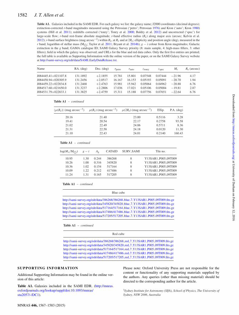
Table A1. Galaxies included in the SAMI EDR. For each galaxy we list: the galaxy name; J2000 coordinates (decimal degrees);extinction-corrected r-band magnitudes measured using the Petrosian (‘petro’; Petrosian 1976) and Kron (‘auto’; Kron 1980)systems (Hill et al. 2011); redshifts corrected (‘tonry’; Tonry et al. 2000; Baldry et al. 2012) and uncorrected (‘spec’) forlarge-scale flow; r-band rest-frame absolute magnitude; r-band effective radius (Re) along major axis (arcsec; Kelvin et al.2012); r-band surface brightness (mag arcsec−2) within Re, at Re and at 2Re; ellipticity and position angle (deg), measured in ther band; logarithm of stellar mass (M�; Taylor et al. 2011; Bryant et al. 2014b); g − i colour from Kron magnitudes; Galacticextinction in the g band; GAMA catalogue ID; SAMI Galaxy Survey priority (8: main sample, 4: high-mass fillers, 3: otherfillers); field in which the galaxy was observed; and URLs for the blue and red data cubes. Only the first five entries are printed;the full table is available as Supporting Information with the online version of the paper, or on the SAMI Galaxy Survey websiteat http://sami-survey.org/edr/data/SAMI EarlyDataRelease.txt.

Name RA. (deg) Dec. (deg) rpetro rauto ztonry zspec Mr Re (arcsec)

J084445.41+021107.8 131.1892 +2.1855 15.781 15.801 0.07548 0.07444 −21.96 4.17J084458.94+020305.9 131.2456 +2.0517 16.167 16.153 0.05193 0.05091 −20.70 1.94J084459.22+022834.8 131.2468 +2.4763 15.981 15.942 0.05064 0.04962 −20.88 6.76J084517.68+021650.0 131.3237 +2.2806 17.036 17.021 0.05106 0.05004 −19.81 2.87J084531.79+022833.1 131.3825 +2.4759 15.311 15.188 0.07756 0.07651 −22.64 6.76

Table A1 – continued

〈μ(Re)〉 (mag arcsec−2) μ(Re) (mag arcsec−2) μ(2Re) (mag arcsec−2) Ellip. P.A. (deg)

20.16 21.40 23.00 0.5116 3.2819.41 20.54 22.17 0.2758 93.5821.02 22.49 24.06 0.5711 8.3621.31 22.58 24.18 0.0120 11.3021.10 22.43 24.01 0.2140 160.43

Table A1 – continued

log(M∗/M�) g − i Ag CATAID SURV SAMI Tile no.

10.95 1.30 0.244 386268 8 Y13SAR1 P005 09T00910.26 1.00 0.316 345820 8 Y13SAR1 P005 09T00910.36 1.02 0.154 517164 8 Y13SAR1 P005 09T00910.09 1.22 0.212 417486 8 Y13SAR1 P005 09T00911.24 1.31 0.165 517205 8 Y13SAR1 P005 09T009

Table A1 – continued

Blue cube

http://sami-survey.org/edr/data/386268/386268 blue 7 Y13SAR1 P005 09T009.fits.gzhttp://sami-survey.org/edr/data/345820/345820 blue 7 Y13SAR1 P005 09T009.fits.gzhttp://sami-survey.org/edr/data/517164/517164 blue 7 Y13SAR1 P005 09T009.fits.gzhttp://sami-survey.org/edr/data/417486/417486 blue 7 Y13SAR1 P005 09T009.fits.gzhttp://sami-survey.org/edr/data/517205/517205 blue 7 Y13SAR1 P005 09T009.fits.gz

Table A1 – continued

Red cube

http://sami-survey.org/edr/data/386268/386268 red 7 Y13SAR1 P005 09T009.fits.gzhttp://sami-survey.org/edr/data/345820/345820 red 7 Y13SAR1 P005 09T009.fits.gzhttp://sami-survey.org/edr/data/517164/517164 red 7 Y13SAR1 P005 09T009.fits.gzhttp://sami-survey.org/edr/data/417486/417486 red 7 Y13SAR1 P005 09T009.fits.gzhttp://sami-survey.org/edr/data/517205/517205 red 7 Y13SAR1 P005 09T009.fits.gz

S U P P O RT I N G IN F O R M AT I O N

Additional Supporting Information may be found in the online ver-sion of this article:

Table A1. Galaxies included in the SAMI EDR. (http://mnras.oxfordjournals.org/lookup/suppl/doi:10.1093/mnras/stu2057/-/DC1).

Please note: Oxford University Press are not responsible for thecontent or functionality of any supporting materials supplied bythe authors. Any queries (other than missing material) should bedirected to the corresponding author for the article.

1Sydney Institute for Astronomy (SIfA), School of Physics, The University ofSydney, NSW 2006, Australia

MNRAS 446, 1567–1583 (2015)

at University of D

urham on February 12, 2016

http://mnras.oxfordjournals.org/

Dow

nloaded from

The SAMI Galaxy Survey: Early Data Release 1583

2ARC Centre of Excellence for All-sky Astrophysics (CAASTRO), 44-70Rosehill Street, Redfern NSW 2016, Sydney, Australia3Australian Astronomical Observatory, PO Box 915, North Ryde, NSW 1670,Australia4Research School of Astronomy & Astrophysics, Australian National Uni-versity, Mount Stromlo Observatory, Cotter road, Weston Creek, ACT 2611,Australia5Department of Physics and Astronomy, University of North Carolina,Chapel Hill, NC 27599, USA6Institute for Astronomy, University of Hawaii, 2680 Woodlawn Drive,Honolulu, HI 96822, USA7Astrophysics Research Institute, Liverpool John Moores University, IC2,Liverpool Science Park, 146 Brownlow Hill, Liverpool L3 5RF, UK8Centre for Astrophysics and Supercomputing, Swinburne University ofTechnology, Hawthorn, VIC 3122, Australia9School of Mathematics and Physics, University of Queensland, QLD 4072,Australia10International Centre for Radio Astronomy Research, University of WesternAustralia, 35 Stirling Highway, Crawley, WA 6009, Australia

11SUPA, School of Physics and Astronomy, University of St Andrews, NorthHaugh, KY16 9SS, UK12ICC, Department of Physics, Durham University, South Road, DurhamDH1 3LE, UK13Institute of Photonics and Optical Science (IPOS), School of Physics, TheUniversity of Sydney, NSW 2006, Australia14European Southern Observatory, Karl-Schwarzschild-Str. 2, D-85748Garching, Germany15Department of Physics and Astronomy, Macquarie University, NSW 2109,Australia16Research Centre for Astronomy, Astrophysics and Astrophotonics, Mac-quarie University, Sydney, NSW 2109 Australia17School of Physics, The University of Melbourne, VIC 3010, Australia18Leibniz-Institut fur Astrophysik Potsdam (AIP), An der Sternwarte 16,D-14482 Potsdam, Germany

This paper has been typeset from a TEX/LATEX file prepared by the author.

MNRAS 446, 1567–1583 (2015)

at University of D

urham on February 12, 2016

http://mnras.oxfordjournals.org/

Dow

nloaded from